Ultra Light OCR Competition Technical Report

1 Introduction

Ultra Light OCR Competition is a Chinese scene text recognition competition jointly organized by CSIG (China Society of Image and Graphics) and Baidu, Inc. In addition to focusing on common problems in Chinese scene text recognition, such as long text length and massive characters, we need to balance the trade-off of model scale and accuracy since the model size limitation in the competition is 10M.

From experiments in aspects of data, model, training, etc., we proposed a general and effective method for Chinese scene text recognition, which got us 2 place among over 100 teams with accuracy 0.817 in TestB dataset. The code is available at https://aistudio.baidu.com/aistudio/projectdetail/2159102.

2 Method

With limited resources(on average, we only had access to 4 NVIDIA 1080Ti graphical cards during this competition) and limited time, we decided to focus on one goal at a time. We start by trying to push up the accuracy, then as the competition moving to the end, we shrink the model with the least accuracy drop we can achieve. Our method can be divided into two parts: Data Analysis and Actual Experiments. We divide our experiments into 3 stages: Over-fitting&baseline, data, model.

2.1 Insights from Data

The dataset provided includes both street-view images(such as shop signs, landmarks, etc.) and images taken from documents and websites. All images provided are rectified to avoid irregular text problems which is a common problem in scene text recognition.

There are a total of 120,000 images provided, of which 100,000 images (with annotations) forms the train set, and the rest are divided into two test sets (TestA/TestB), each with 10,000 images (without annotations).

We randomly divide the train set provided into train/val set with ratio 9:1 for the convenience of subsequent experiments and analysis since online submissions for TestA are limited to 5 times a day.

2.1.1 Annotation

Distinct characters

The numbers of distinct characters in the train set and val set were shown in Table 1. As anticipated, the number of possible characters is enormous. Note that there are a total of 66 characters(from 63 text samples) that only appear in the val set, which would induce 0.63% accuracy loss theoretically.

	Number of Distinct Characters
Train Set	3908
Val Set	2516
Total	3974

Table 1: Number of Distinct Characters across Train/Val Set

Character Frequency

As shown in Table 2, we found that, in terms of character frequency, the long-tail problem is significant. Note that around 1/5 characters appeared only once.

	1000+	100-1000	10-100	1-10	1	Total
Train	86(2.2%)	783(20.0%)	1246(31.9%)	1138(29.1%)	655(16.8%)	3908
Val	3(0.1%)	99(3.9%)	812(32.3%)	1037(41.2%)	565(22.5%)	2516
Total	100	828	1262	1116	668	6424

Table 2: Character Frequency in Train/Val Set

Text Length

As shown in Figure 1, most of text samples have length in range 1 to 22. Here we only show the text length distribution for train set since val set has similar distribution as train set.

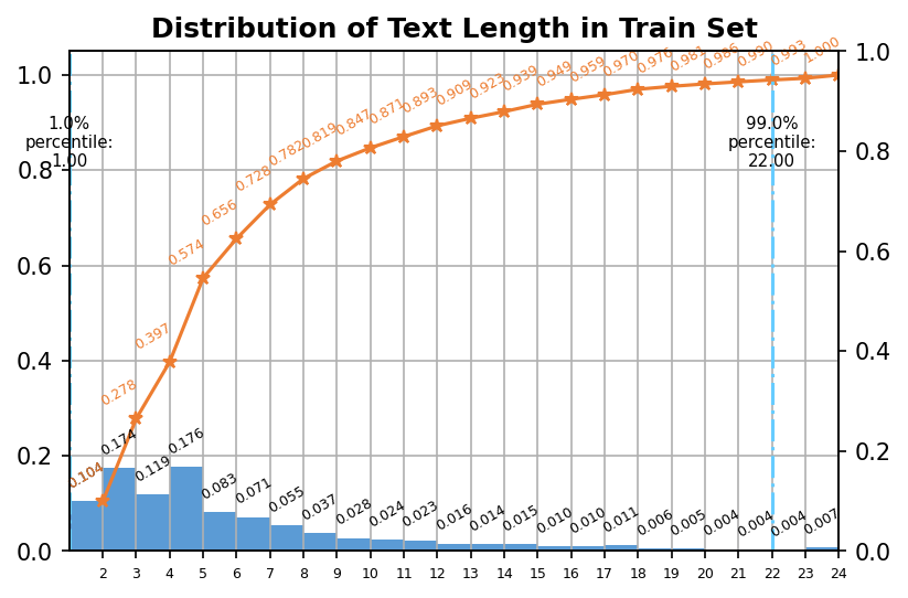
Figure 1: Distribution of Text Length in Train Set

Label Noise

We random sampled and eyeballed 500 images from train set and noticed that 17 of them were mislabeled. This means that there are noises in train/val set and potentially in test set. As a result, theoretically, assuming there are noises of same level in the test set, a perfect model would suffer a 3.4% accuracy loss.

2.1.2 Image

Image Scale

The scale of images in train set is shown in Figure 2. As expected, most images have longer width than height. We also notice that the aspect ratio of the dataset is limited in certain range since all the image in the dataset form two clear slop in the figure.

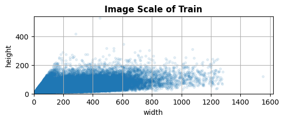
Figure 2: Image Scale Distribution of Train Set

Image Height

As for the height, as showed in Figure 3, the height of 39.4% of the images are greater than 32 pixels, 21.6% are greater than 48 pixels, and 13.1% are greater than 64 pixels.

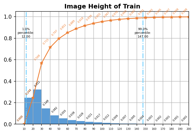
Figure 3: Image Height in Train Set

2.2 Experiment stages

2.2.1 Baseline

We called this stage ‘over-fitting&baseline’ earlier because we’d like to emphasize the importance of fitting the train set. Here, over-fitting refers to a set of experiments that tries to ‘over-fit’ the model on the train set. These experiments are conducted on different subsets of training set: starting from a single image to a batch of images, to a larger portion of the train set, and eventually the whole train set. The goal of those experiments is to spot problems in the early stage. For instance, if a model cannot even over-fit on only one batch of images, it’s obvious that there is something wrong in the training process: not enough model capacity? Inappropriate hyper-parameters? Some special cases of data that you are not aware of?

We start over-fitting experiments with settings below:

Training Framework

According to the competition regulations, our only choice is PaddleOCR.

Algorithm

Although the attention-based prediction approaches have become the mainstream method in the field of scene text recognition, we choose CTC-based method after survey investigation because of its strength on dealing with long text sequences and large-scale category recognition tasks[1].

We use CRNN[2] as our OCR framework, the architecture is shown in Figure 4.

Figure 4: Architecture of the CRNN Algorithm

Data Augmentation Design

We first studied the starter code provided in the competition and noticed the data augmentation provided baseline in PaddleOCR is not applicable for reasons below:

• The provided augmentation setting does not align to data distribution as in our point of view.

• The implementation is ill-designed: everything were coupled in a single function, which make it inconvenient for subsequent controlled experiment.

Based on the reasons above, we decide to redesign the data augmentation module. Note that we removed all data augmentations in over-fitting experiments to eliminate the inference from those augmentations. Input images are resized to 32 × 320 without any further augmentations.

Limit Character Category

Default category provided by PaddleOCR consists of 6623 characters.

• As shown in Table 1, since there are only 3974 unique characters in provided dataset, there is no need to keep characters that are not in the train set. This reduces the number of parameters and memory usage without any accuracy loss.

• We noticed that the space character contributes nothing during metric calculation in the competition, so we also removed the space characters from the Character Set.

Input/Output Setting

The size of input images is set to 32 × 320. And the max length of output sequence is set to 25 since the longest text in the data set is 24.

Model Architecture

Same as the default setting, we use MobileNetV3-Small[3] with multipliers 0.5 as backbone, A two-layer BiLSTM with hidden size 48 as Neck(sequence encoder) and a fully connected layer as head.

Loss Function

We adopt CTC loss proposed by Graves et al.[4] as the loss function.

Training

We used Adam optimizer with cosine annealing with warm restarts:

• Initial learning rate: $2e^{-3}$

• Total training epoch: $2000$

• Restart period: every $50$ epoch

	Base Model	Large Model
Accuracy	0.8096	1.0

Table 3: Accuracy between different model capacity on Train Set

The settings above(called Base Model in Table 3) didn’t over-fit the train set well. Conjecturing that here model capacity is the main shortcoming, we enlarged model capacity and did the experiment again:

• Backbone: MobileNetV3-Large with multipliers $1.0$

• Neck: Increasing the hidden size of BiLSTM from $48$ to $256$

As shown in Table 3, the increase of model capacity brings training accuracy to $1.0$ which means it is more than enough for fitting the train set. We then continue to evaluate the accuracy on the val set. As shown in Table 4, although the large model totally fitted the train set, the val accuracy seems acceptable. Since we plan to focus on accuracy first and shrink model size in the later stage, we choose this enlarged model as our baseline.

	Base Model	Large Model
Accuracy	0.5949	0.7494

Table 4: Accuracy between different model capacity on Val Set

2.2.2 Data

As data matters a lot, we start data-related experiments right after we got our baseline. At this stage, our goal is to further improve accuracy. Based on our observation and analysis, we conducted experiments on data augmentation and input image scale.

For data augmentation, we focused on geometry transforms, noises, and color transforms. In natural scenes, text appears in various shapes and distorted patterns. In addition, the phenomenon of occlusion is also a big challenge for text recognition. The general approaches are adding data augmentation like Crop, Rotate, Cutout, TIA[5], etc. Noise, on the other hand, happens all the time in the real world, such as non-uniform illumination, blurring and electrical noises. We added different kinds of noise, blur to mimic them. Last but not least, to enrich color distribution in the dataset, we added some color-related transforms. Data augmentations we used are listed below:

Random Height Crop

We randomly crop the top or bottom of the image with respect to the Image size, the crop ratio is between 0 and 0.05.

Cutout

In order to alleviate the problem of text occlusion, We randomly replace 1 to 3 areas with random colors according to the image size, the ratio is between 0.05 and 0.1.

TIA

TIA[5] is a data augmentation which is more effective and specific for training a robust recognizer. A set of fiducial points are initialized on the image, then these points are randomly be moved to generate new image with the geometric transformation, such as distortion, stretch and perspective. The number of initial fiducial points is randomly set between 3 and 6.

GaussNoise

We apply Gaussian noise with mean = 0 and standard deviation randomly between 0 and 10.

MotionBlur

We apply motion blur with kernel size between 3 and 7.

Order of augmentations

During data experiments, we adjusted the order of data augmentation:

• Blurriness is influenced by the scale of the image. The effect of same blur kernel on different sized images differs a lot. If even a human eye can not recognize a blurred character, there is no way a model can recognize it. So we decide to put the MotionBlur after image resize to make sure same kernel is applied to images with same scale.

• The gaussian noise after blur looks very different from data distribution in the val set. Our experiment also proves that put GaussNoise before MotionBlur is a better choice.

Aside from data augmentations mentioned, we adjusted the input size based on the analysis shown in Figure 3: the height of $21.6\%$ of the images is greater than 48 pixels. To reduce information loss in the process of resize, we increased the input scale:

Input Scale

increase the input scale from 32 × 320 to 48 × 480 (Being limited by our hardware, we do not further increase the input scale).

A summary of experiments in this stage can be found in Table 5.

Baseline∗	✓	✓	✓	✓	✓	✓	✓
Random Height Crop		✓	✓	✓	✓	✓	✓
Cutout			✓	✓	✓	✓	✓
TIA				✓	✓	✓	✓
GaussNoise					✓	✓	✓
MotionBlur						✓	✓
Input Scale							✓
Accuracy	0.7494	0.7531	0.7588	0.7654	0.7679	0.7689	0.8039

^∗ Baseline is best model(Large Model) last Stage

Table 5: Accuracy of Experiments on Data

2.2.3 Model

This stage can be divide into two parts: higher accuracy, smaller model.

We noticed that in the backbone, the image is only down-sampled at the beginning and the end horizontally. Since, as shown in Figure 2, images are likely to be wider instead of taller, we speculate that the horizontal receptive field is not enough for this task. So we adjusted the receptive field:

Larger Receptive Field

In the first layer of the C2 stage of the backbone, we modified the stride of the down-sampling feature map from (2,1) to (2,2), which increases the receptive field horizontally.

Also, as the model is able to $100\%$ fit the train set in early experiments, we conjecture that our model is still suffering from over-fitting to some degree although a lot of augmentations were introduced.

Back to Lightweight Model

Being required to submit a model less than 10M, we choose lowering the amount of parameters as our first attempt to reduce over-fitting. We decrease the multipliers of MobileNetV3-Large from 1.0 to 0.6 and cut down the hidden size of BiLSTM from 256 to 64. The number of parameters is reduced to 9.5M, which meets the requirements of the competition. Unexpectedly, as shown in Table 6, we found that decreasing the multipliers aggravated over-fitting (val-accuracy dropped significantly while train-accuracy maintained roughly the same). We speculate that the reason behind this is model-wise double decent phenomena as explained in [6] (By reducing parameters, our model are approaching ’Interpolation Threshold’ from ’Modern Regime’).

	Large Model	Light Model
Train	0.9992	0.9957
Val	0.8087	0.7874

Table 6: Accuracy between Large and Light Model

Spatial Dropout

We applied spatial dropout [7] in all layers on C5 stage on backbone with $keep\_prob=0.9$.

Weight Decay

We increased weight decay of the fully connected layer form $1e^{-5}$ to $4e^{-5}$.

A summary of results in this stage can be found in Table 7.

Fusion∗	✓	✓	✓	✓	✓
Larger Receptive Field		✓	✓	✓	✓
Light Model			✓	✓	✓
Spatial Dropout				✓	✓
Weight Decay					✓
Accuracy	0.8039	0.8087	0.7847	0.8045	0.8112

^∗ Fusion is best model in Data Experiments

Table 7: Accuracy of Experiments on Model

3 Full Dataset Training

Generally we would like to do a cross-validation before using full data. However, due to limited time and machine, we trained the model on full dataset and submitted the checkpoint from the latest epoch in the end.

4 Things We Tried But Didn’t Work

ColorJitter

Randomly changes the brightness, contrast, saturation, and hue of an image with default parameter setting from Albumentation[8].

Pixel Reverse

Randomly reverse all the pixel of image.

Random Rotate

Rotate the image with a random degree between $(-10^{\circ},10^{\circ})$, and then resize the image to keep all pixels are still in the region of image.

Multi-Scale Feature Fusion

Concatenate the feature map for C3, C4 and C5 stage to merge low-level and high-level semantics.

Multi-Scale Training

Randomly select one from the following three scales ([32, 320], [48, 480] and [64, 640]) as the input scale during training, and replace the last pooling layer of the backbone to AdaptivePool to ensure that the size of the feature map is consistent. We switched scale every 8 iters during training.

Test Time Augmentation(TTA)

During inference stage we tried to use TTA on the multi-scale-trained model. We get predictions from the three scales mentioned above, and select the prediction with highest score as the final result. We also tried to average the predicted probabilities of the three before decoding, however these two methods did not bring any improvement.

Beam Search

In decode module we use Greedy Search algorithm which selects one best candidate as an input sequence for each time step. However, choosing just one best candidate might be suitable for the current time step, but when we construct the full sentence, it may be a sub-optimal choice.

Based on this consideration, we tried to use Beam Search algorithm which selects multiple alternatives for an input sequence at each time step based on conditional probability. We tried different beam width, but none of them works.

5 Conclusion

Conclusively, we adopt CTC-based architecture, input scale of 48 × 480, series of data augmentation and anti-over-fitting methods, achieved 81.7% on TestB data set in Ultra Light OCR Competition. We believe with more resources and time, the score could be further improved.

References

- [1] Xiaoxue Chen, Lianwen Jin, Yuanzhi Zhu, Canjie Luo, and Tianwei Wang. Text recognition in the wild: A survey. CoRR, abs/2005.03492, 2020.
- [2] Baoguang Shi, Xiang Bai, and Cong Yao. An end-to-end trainable neural network for image-based sequence recognition and its application to scene text recognition. CoRR, abs/1507.05717, 2015.
- [3] Andrew Howard, Mark Sandler, Grace Chu, Liang-Chieh Chen, Bo Chen, Mingxing Tan, Weijun Wang, Yukun Zhu, Ruoming Pang, Vijay Vasudevan, Quoc V. Le, and Hartwig Adam. Searching for mobilenetv3. CoRR, abs/1905.02244, 2019.
- [4] Alex Graves, Santiago Fernández, Faustino Gomez, and Jürgen Schmidhuber. Connectionist Temporal Classification: Labelling Unsegmented Sequence Data with Recurrent Neural Networks. In Proceedings of the 23rd International Conference on Machine Learning, ICML ’06, pages 369–376, New York, NY, USA, 2006. ACM.
- [5] Canjie Luo, Yuanzhi Zhu, Lianwen Jin, and Yongpan Wang. Learn to augment: Joint data augmentation and network optimization for text recognition. CoRR, abs/2003.06606, 2020.
- [6] Preetum Nakkiran, Gal Kaplun, Yamini Bansal, Tristan Yang, Boaz Barak, and Ilya Sutskever. Deep double descent: Where bigger models and more data hurt. arXiv preprint arXiv:1912.02292, 2019.
- [7] Jonathan Tompson, Ross Goroshin, Arjun Jain, Yann LeCun, and Christoph Bregler. Efficient object localization using convolutional networks. In Proceedings of the IEEE conference on computer vision and pattern recognition, pages 648–656, 2015.
- [8] Alexander Buslaev, Vladimir I. Iglovikov, Eugene Khvedchenya, Alex Parinov, Mikhail Druzhinin, and Alexandr A. Kalinin. Albumentations: Fast and flexible image augmentations. Information, 11(2), 2020.