Linear Contextual Bandits with Adversarial Corruptions

Abstract

We study the linear contextual bandit problem in the presence of adversarial corruption, where the interaction between the player and a possibly infinite decision set is contaminated by an adversary that can corrupt the reward up to a corruption level $C$ measured by the sum of the largest alteration on rewards in each round. We present a variance-aware algorithm that is adaptive to the level of adversarial contamination $C$. The key algorithmic design includes (1) a multi-level partition scheme of the observed data, (2) a cascade of confidence sets that are adaptive to the level of the corruption, and (3) a variance-aware confidence set construction that can take advantage of low-variance reward. We further prove that the regret of the proposed algorithm is $\widetilde{O}(C^{2}d\sqrt{\sum_{t=1}^{T}\sigma_{t}^{2}}+C^{2}R\sqrt{dT})$, where $d$ is the dimension of context vectors, $T$ is the number of rounds, $R$ is the range of noise and $\sigma_{t}^{2},t=1\ldots,T$ are the variances of instantaneous reward. We also prove a gap-dependent regret bound for the proposed algorithm, which is instance-dependent and thus leads to better performance on good practical instances. To the best of our knowledge, this is the first variance-aware corruption-robust algorithm for contextual bandits. Experiments on synthetic data corroborate our theory.

1 Introduction

Multi-armed bandit algorithms are widely applied in online advertising (Li et al., 2010), clinical trials (Villar et al., 2015), recommendation system (Deshpande and Montanari, 2012) and many other real-world tasks. In the model of multi-armed bandits, the algorithm needs to decide which action (or arm) to take (or pull) at each round and receives a reward for the chosen action. In the stochastic setting, the reward is subject to a fixed but unknown distribution for each action. In reality, however, these rewards can easily be “corrupted” by some malicious users. A typical example is click fraud (Lykouris et al., 2018), where botnets simulate the legitimate users clicking on an ad to fool the recommendation systems. This motivates the studies of bandit algorithms that are robust to adversarial corruptions. For example, Lykouris et al. (2018) introduced a bandit model in which an adversary could corrupt the stochastic reward generated by an arm pull. They proposed an algorithm and showed that the regret of the algorithm degrades smoothly as the amount of corruption diminishes. Gupta et al. (2019) proposed an alternative algorithm which gives a significant improvement in regret.

While the algorithms that are robust to the corruptions have been studied in the setting of multi-armed bandits in a number of prior works, they are still understudied in the setting of linear contextual bandits. The linear contextual bandit problem can be regarded as an extension of the multi-armed bandit problem to linear optimization, in order to tackle an unfixed and possibly infinite set of feasible actions. There is a large body of literature on efficient algorithms for linear contextual bandits without corruptions (Abe et al., 2003; Auer, 2002; Dani et al., 2008; Li et al., 2010; Rusmevichientong and Tsitsiklis, 2010; Chu et al., 2011; Abbasi-Yadkori et al., 2011; Li et al., 2019b), to mention a few. The significance of this setting lies in the fact that in real world applications, arms often come with contextual information that can be utilized to facilitate arm selection (Li et al., 2010; Deshpande and Montanari, 2012; Jhalani et al., 2016). Linear contextual bandits with adversarial corruptions is an arguably more challenging setting since most of the previous corruption-robust algorithms are based on the idea of action elimination (Lykouris et al., 2018; Gupta et al., 2019; Bogunovic et al., 2021), which is not applicable to the contextual bandit settings where the decision set is time varying and possibly infinite at each round. Garcelon et al. (2020) showed that a malicious agent can force a linear contextual bandit algorithm to take any desired action $T-o(T)$ times over $T$ rounds, while applying adversarial corruptions to rewards with a cumulative cost that only grow logarithmically. This poses a big challenge for designing corruption-robust algorithms for linear contextual bandits.

In this paper, we make a first attempt to study a linear contextual bandit model where an adversary can corrupt the rewards up to a corruption level $C$, which is defined as the the sum of biggest alteration on the reward the adversary makes in each round. We propose a linear contextual bandit algorithm that is robust to reward corruption, dubbed multi-level optimism-in-the-face-of-uncertainty weighted learning (Multi-level weighted OFUL). More specifically, our algorithm consists of the following novel techniques: (1) We design a multi-level partition scheme and adopt the idea of sub-sampling to perform a robust estimation of the model parameters; (2) We maintain a cascade of candidate confidence sets corresponding to different corruption level (which is unknown) and randomly select a confidence set at each round to take the action; and (3) We design confidence sets that depend on the variances of rewards, which lead to a potentially tighter regret bound.

Our contributions are summarized as follows:

• We propose a variance-aware algorithm which is adaptive to the amount of adversarial corruptions $C$. To the best of our knowledge, it is the first algorithm for the setting of linear contextual bandits with adversarial corruptions which does not rely on the finite number of actions and other additional assumptions.

• We prove that the regret of our algorithm is $\widetilde{O}\left(C^{2}d\sqrt{\sum_{t=1}^{T}\sigma_{t}^{2}}+C^{2}R\sqrt{dT}\right)$, where $d$ is the dimension of context vectors, $T$ is the number of rounds, $R$ is the range of noise and $\sigma_{t}^{2},t=1\ldots,T$ are the variances of instantaneous reward. Our regret upper bound has a multiplicative dependence on $C^{2}$ which indicates that our algorithm achieves a sub-linear regret when the corruption level satisfies $C=o(T^{1/4})$.

• We also derive a gap-dependent regret bound $\widetilde{O}\left(\frac{1}{\Delta}\cdot C^{2}R^{2}d+\frac{1}{\Delta}\cdot d^{2}C^{2}\max_{t\in[T]}\sigma_{t}^{2}\right)$ for our proposed algorithm, which is instance-dependent and thus leads to a better performance on good instances.

Concurrent to our work, Ding et al. (2021) also studied linear contextual bandits under adversarial attacks where the adversary can attack on the rewards. However, a careful examination of their proof finds that their proof is flawed, and their seemingly better regret is questionable.

Notation.

We use lower case letters to denote scalars, and use lower and upper case bold face letters to denote vectors and matrices respectively. We denote by $[n]$ the set $\{1,\dots,n\}$. For a vector $\mathbf{x}\in\mathbb{R}^{d}$ and matrix $\bm{\Sigma}\in\mathbb{R}^{d\times d}$, a positive semi-definite matrix, we denote by $\|\mathbf{x}\|_{2}$ the vector’s Euclidean norm and define $\|\mathbf{x}\|_{\bm{\Sigma}}=\sqrt{\mathbf{x}^{\top}\bm{\Sigma}\mathbf{x}}$. For two positive sequences $\{a_{n}\}$ and $\{b_{n}\}$ with $n=1,2,\dots$, we write $a_{n}=O(b_{n})$ if there exists an absolute constant $C>0$ such that $a_{n}\leq Cb_{n}$ holds for all $n\geq 1$ and write $a_{n}=\Omega(b_{n})$ if there exists an absolute constant $C>0$ such that $a_{n}\geq Cb_{n}$ holds for all $n\geq 1$. We use $\widetilde{O}(\cdot)$ to further hide the polylogarithmic factors. We use $\operatorname{\mathds{1}}(\cdot)$ to denote the indicator function.

2 Related Work

Bandits with Adversarial Rewards: There is a large body of literature on the problems of multi-armed bandits in the adversarial setting (See Auer et al. (2002); Bubeck and Cesa-Bianchi (2012) and references therein). Many recent efforts in this area aim to design algorithms that achieve desirable regret bound in both stochastic multi-armed bandits and adversarial bandits simultaneously, known as “the best of both worlds” guarantees (Bubeck and Slivkins, 2012; Seldin and Slivkins, 2014; Auer and Chiang, 2016; Seldin and Lugosi, 2017; Zimmert and Seldin, 2019). These works mainly focus on achieving sublinear regret in the worst case and the case where there is no adversary. As a result, these algorithms are either not robust to instances with moderate amount of corruptions, or suffer from restrictive assumptions on adversarial corruptions (e.g., Seldin and Slivkins (2014) and Zimmert and Seldin (2019) assumed that the adversarial corruptions do not reduce the gap by more than a constant factor at any point of time). Different from the above line of research, Lykouris et al. (2018) studied a variant of classic multi-armed bandit model in the “middle ground”, where each pull of an arm generates a stochastic reward that may be contaminated by an adversary before it is revealed to the player. In their work, the corruption level $C$ is defined as $C=\sum_{t}\max_{a}|r^{t}(a)-r_{\mathcal{S}}^{t}(a)|$ where $r_{\mathcal{S}}^{t}(a)$ is the stochastic reward of arm $a$ and $r^{t}(a)$ is the corrupted reward of arm $a$ at round $t$. They proposed an algorithm that is adaptive to the unknown corruption level, which achieves an $O(K^{1.5}C\sqrt{T})$ regret bound. Gupta et al. (2019) proposed an improved algorithm that can achieve a regret bound with only additive dependence on $C$. On the flip side, many research efforts have also been devoted into designing adversarial attacks that cause standard bandit algorithms to fail (Jun et al., 2018; Liu and Shroff, 2019; Lykouris et al., 2018; Garcelon et al., 2020).

Stochastic Linear Bandits with Corruptions: Li et al. (2019a) studied stochastic linear bandits with adversarial corruptions and achieved $\widetilde{O}(d^{5/2}C/\Delta+d^{6}/\Delta^{2})$ regret bound where $d$ is the dimension of the context vectors, $\Delta$ is the gap between the rewards of the best and the second best actions in the decision set $\mathcal{D}$. Bogunovic et al. (2021) also studied corrupted linear bandits with a fixed decision set of $k$ arms and obtained $\widetilde{O}(\sqrt{dT}+Cd^{3/2}+C^{2})$ regret upper bound. Recently, Lee et al. (2021) considered corrupted linear bandits with a finite and fixed decision set and achieved a regret of $\widetilde{O}(d\sqrt{T}+C)$. While both Lee et al. (2021) and Li et al. (2019a) focused on corrupted linear stochastic bandits, Lee et al. (2021) used a slightly different definition of regret and adopted a strong assumption on corruptions that at each round $t$, the corruptions on rewards are linear in the actions.

Linear Contextual Bandits with Corruptions: Bogunovic et al. (2021) studied linear contextual bandits with adversarial corruptions and considered the setting under the assumption that context vectors undergo small random perturbations, which is previously introduced by Kannan et al. (2018). Besides the additional assumption, another major distinction in Bogunovic et al. (2021) is that the number of actions $k$ is finite and the regret bound depends on $k$ in the contextual setting with unknown corruption level $C$. Neu and Olkhovskaya (2020) studied misspecified linear contextual bandits with a finite decision set (i.e., $K$ actions) and proved an $\widetilde{O}((Kd)^{\frac{1}{3}}T^{\frac{2}{3}})+\epsilon\cdot\sqrt{d}T$ regret bound for their proposed algorithm. Kapoor et al. (2019) considered the corrupted linear contextual bandits under an assumption on corruptions that for any prefix, at most an $\eta$ fraction of the rounds are corrupted.

3 Preliminaries

We will introduce our model and some basic concepts in this section.

Corrupted linear contextual bandits. We consider the the linear contextual bandits model studied in Abbasi-Yadkori et al. (2011) under the same corruption studied by Lykouris et al. (2018). In detail, distinctive from the linear contextual bandits Abbasi-Yadkori et al. (2011), the interaction between the agent and the environment is now contaminated by an adversary. The protocol between the agent and the adversary at each round $t\in[T]$ is described as follows: 1. At the beginning of round $t$, the environment generates an arbitrary decision set $\mathcal{D}_{t}\subseteq\mathbb{R}^{d}$ where each element represents a feasible action that can be selected by the agent. 2. The environment generates stochastic reward function $r_{t}^{\prime}(\mathbf{a})=\langle\mathbf{a},\bm{\mu}^{*}\rangle+\epsilon_{t}(\mathbf{a})$ together with an upper bound on the standard variance of $\epsilon_{t}(\mathbf{a})$, i.e., $\sigma_{t}(\mathbf{a})$ for all $\mathbf{a}\in\mathcal{D}_{t}$. 3. The adversary observes $\mathcal{D}_{t}$, $r_{t}^{\prime}(\mathbf{a})$, $\sigma_{t}(\mathbf{a})$ for all $\mathbf{a}\in\mathcal{D}_{t}$ and decides a corrupted reward function $r_{t}$ defined over $\mathcal{D}_{t}$. 4. The agent observes $\mathcal{D}_{t}$ and selects $\mathbf{a}_{t}\in\mathcal{D}_{t}$. 5. The adversary observes $\mathbf{a}_{t}$ and then returns $r_{t}(\mathbf{a}_{t})$ and $\sigma_{t}(\mathbf{a}_{t})$. 6. The agent observes $r_{t}(\mathbf{a}_{t}),\sigma_{t}(\mathbf{a}_{t})$.

Let $\mathcal{F}_{t}$ be the $\sigma$-algebra generated by $\mathcal{D}_{1:t},\mathbf{a}_{1:t-1},\epsilon_{1:t-1},r_{1:t-1}$ and $\sigma_{1:t-1}$.

At step 2, $\bm{\mu}^{*}$ is a hidden vector unknown to the agent which can be observed by the adversary at the beginning. We assume that for all $t\geq 1$ and all $\mathbf{a}\in\mathcal{D}_{t}$, $\|\mathbf{a}\|_{2}\leq A$, $|\langle\mathbf{a},\bm{\mu}^{*}\rangle|\leq 1$ and $\|\bm{\mu}^{*}\|_{2}\leq B$ almost surely. $\epsilon_{t}(\mathbf{a})$ can be any form of random noise as long as it satisfies

$$\forall t\geq 1, \forall\mathbf{a}\in\mathcal{D}_{t},|\epsilon_{t}(\mathbf{a})|\leq R,\quad\mathbb{E}[\epsilon_{t}(\mathbf{a})|\mathcal{F}_{t}]=0,\mathbb{E}[\epsilon_{t}^{2}(\mathbf{a})|\mathcal{F}_{t}]\leq\sigma_{t}^{2}(\mathbf{a}).$$ (3.1)

This assumption on $\epsilon_{t}$ is a variant of that in Zhou et al. (2020): Here we require the noise to be generated for all $\mathbf{a}\in\mathcal{D}_{t}$ in advance before the adversary decides the corrupted reward function. Our assumption on noises is more general than those in Li et al. (2019a); Bogunovic et al. (2021); Kapoor et al. (2019) where the noises are assumed to be 1-sub-Gaussian or Gaussian. The motivation behind this assumption is that the environment may change over time in practical applications. Also, on the theoretical aspect, the setting of heteroscedastic noise is more general and can be extended to the Markov decision processes (MDPs) in reinforcement learning (Zhou et al., 2020), where the “noise” is caused by the transition of states and the variance can be estimated by the agent.

At step 3, the adversary has observed all the previous information and thus may predict which policy the agent will take at the current round. However, since the agent can take a randomized policy, the adversary may not know exactly which action the agent will take.

Corruption level. We define corruption level

$$C=\frac{1}{R+1}\sum_{t=1}^{T}\sup_{\mathbf{a}\in\mathcal{D}_{t}}|r_{t}^{\prime}(\mathbf{a})-r_{t}(\mathbf{a})|.$$ (3.2)

to indicate the level of adversarial contamination. We say a model is $C$-corrupted if the corruption level is no larger than $C$.

Our definition of corruption level is equivalent to the counterpart in Lykouris et al. (2018) and Gupta et al. (2019) where they define $C=\sum_{t=1}^{T}\max_{\mathbf{a}}|r_{t}^{\prime}(\mathbf{a})-r_{t}(\mathbf{a})|$ in our notation of rewards. We introduce a normalization factor of $R+1$ since the noise is of range $R$ in our model, while they assume all the rewards are in range $[0,1]$.

Regret. Since the actions selected by the agent may not be deterministic, we define the regret for this model as follows:

$$\mathbf{Regret}(T)=\sum_{t=1}^{T}\langle\mathbf{a}_{t}^{*},\bm{\mu}^{*}\rangle-\mathbb{E}\left[\sum_{t=1}^{T}\langle\mathbf{a}_{t},\bm{\mu}^{*}\rangle\right].$$ (3.3)

Our definition follows from the definition in Gupta et al. (2019) where the pseudo-regret (a standard metric in stochastic multi-armed bandit models of) is adopted. It is worth noting that we need to take the expectation on $\sum_{t=1}^{T}r_{t}^{\prime}(\mathbf{a}_{t})$ (the second term in (3.3)), since a randomized policy is applied in each round.

Gap. Let $\Delta_{t}$ be the gap between the rewards of the best and the second best actions in the decision set $\mathcal{D}_{t}$ as defined in Dani et al. (2008) which can be formally written as

$$\Delta_{t}=\min_{\mathbf{a}\in\mathcal{D}_{t},\mathbf{a}\not\in\mathcal{A}_{t}^{*}}\left(\langle\mathbf{a}_{t}^{*},\bm{\mu}^{*}\rangle-\langle\mathbf{a},\bm{\mu}^{*}\rangle\right).$$ (3.4)

where $\mathcal{A}_{t}^{*}=\mathop{\mathrm{argmax}}_{\mathbf{a}\in\mathcal{D}_{t}}\langle\mathbf{a},\bm{\mu}^{*}\rangle$ and $\mathbf{a}_{t}^{*}$ is an arbitrary element in $\mathcal{A}_{t}^{*}$. Let $\Delta$ denotes the smallest gap $\min_{t\in[T]}\Delta_{t}$.

4 Warm up: Algorithm for Known Corruption Level

Algorithm 1 Robust weighted OFUL

1:  Set $\bm{\Sigma}_{1}\leftarrow\lambda\mathbf{I},\bm{\mu}_{1}\leftarrow{\bm{0}},\mathbf{c}_{1}\leftarrow 0.$

2:  for $\ell=1,\cdots,T$ do

3:     Observe $\mathcal{D}_{t}$.

4:     Set $\mathcal{C}_{t}$ as defined in (4.1).

5:     Select $\mathbf{a}_{t}\leftarrow\mathop{\mathrm{argmax}}_{\mathbf{a}\in\mathcal{D}_{t}}\max_{\bm{\mu}\in\mathcal{C}_{t}}$ and observe $r_{t},\sigma_{t}$.

6:     Set $\overline{\sigma}_{t}=\max\{(R+1)/\sqrt{d},\sigma_{t}\}.$

7:     Update estimator: $\bm{\Sigma}_{t+1}\leftarrow\bm{\Sigma}_{t}+\mathbf{a}_{t}\mathbf{a}_{t}^{\top}/\overline{\sigma}_{t}^{2}$, $\mathbf{c}_{t+1}\leftarrow\mathbf{c}_{t}+r_{t}\mathbf{a}_{t}/\overline{\sigma}_{t}^{2}$, $\bm{\mu}_{t+1}\leftarrow\bm{\Sigma}_{t+1}^{-1}\mathbf{c}_{t+1}.$

8:  end for

In this section, we show that if the corruption level $C$ is revealed to the agent, a robust version of weighted OFUL (Abbasi-Yadkori et al., 2011; Zhou et al., 2020) in Algorithm 1 can achieve a regret upper bound of $\widetilde{O}(CRd\sqrt{T})$.

The key idea is that we use an enlarged confidence bound to adapt to the known corruption level $C$:

$$\mathcal{C}_{t}=\{\bm{\mu}|\|\bm{\mu}-\bm{\mu}_{t}\|\leq\alpha_{t}\}$$ (4.1)

where

$$\alpha_{t} =8\sqrt{d\log\frac{(R+1)^{2}\lambda+tA^{2}}{(R+1)^{2}\lambda}\log(4t^{2}/\delta)}$$

$$\quad+4\sqrt{d}\log(4t^{2}/\delta)+C{\sqrt{d}}+\sqrt{\lambda}B.$$ (4.2)

Lemma 4.1 (Enlarged Confidence Ellipsoid. ).

With probability at least $1-\delta$, we have $\bm{\mu}^{*}\in\mathcal{C}_{t}$ for all $t\geq 1$.

According to the above lemma, we can compute such enlarged confidence ellipsoids at each round $t$ to ensure that $\bm{\mu}^{*}$ is still in the confidence sets under adversarial attacks if we know the corruption level in advance.

With the enlarged confidence sets, we show that Algorithm 1 achieves a regret upper bound adapting to the known corruption level $C$ in the following theorem.

Theorem 4.2.

Set $\lambda=1/B^{2}$. Suppose $C=\Omega(1),R=\Omega(1)$, for all $t\geq 1$ and all $\mathbf{a}\in\mathcal{D}_{t}$, $\langle\mathbf{a},\bm{\mu}^{*}\rangle\in[-1,1]$. Then with probability at least $1-\delta$, the regret of Algorithm 1 is bounded as follows:

$$\mathbf{Regret}(T)=\widetilde{O}\left(Cd\sqrt{\sum_{t=1}^{T}\sigma_{t}^{2}}+CR\sqrt{dT}\right).$$ (4.3)

Remark 4.3.

Theorem 4.2 suggests that when the corruption level $C$ is known, Algorithm 1 incurs a regret that has a linear dependence on $C$. On the other hand, if we trivially upper bound $\sigma_{t}$’s by $R$, the regret of Algorithm 1 degenerates to $\widetilde{O}\left(CdR\sqrt{T}\right)$. This suggests that the use of variance information can lead to a tighter regret bound.

Remark 4.4.

When $\sigma_{t},R=\Omega(1)$, the regret bound in Theorem 4.2 matches the regret bound of weighted OFUL proposed in Zhou et al. (2020) when the corruption level $C$ is a constant.

5 Algorithm for Unknown Corruption Level

In this section, we propose an algorithm, Multi-level weighted OFUL, in Algorithm 2, to tackle the corrupted linear contextual bandit problem with unknown corruption level. At the core of our algorithm is an action partition scheme to group historical selected actions and use them to select the future actions in different groups with different probabilities. Such a scheme is introduced to deal with the unknown corruption level. For simplicity, we denote $r_{t}(\mathbf{a}_{t}),\sigma_{t}(\mathbf{a}_{t})$ in Section 3 by $r_{t},\sigma_{t}$ in our algorithm.

Algorithm 2 Multi-level weighted OFUL

1:  Set the largest level of confidence sets: $\ell_{\max}\leftarrow\lceil\log_{2}2T\rceil$.

2:  For $\ell\in[\ell_{\max}]$, set $\bm{\Sigma}_{1,\ell}\leftarrow\lambda\mathbf{I},\bm{\mu}_{1,\ell}\leftarrow{\bm{0}},\mathbf{c}_{1,\ell}\leftarrow{\bm{0}}.$

3:  Set $\bm{\Sigma}_{1}\leftarrow\lambda\mathbf{I},\bm{\mu}_{1}\leftarrow{\bm{0}},\mathbf{c}_{1}\leftarrow{\bm{0}}.$

4:  for $t=1,\cdots,T$ do

5:     Observe $\mathcal{D}_{t}.$

6:     for $\ell=1,\cdots,\ell_{\max}$ do

7:        Set $\beta_{t,\ell}$ and $\gamma_{t,\ell}$ as defined in (5.4) and (5.5).

8:        $\mathcal{C}_{t,\ell}^{\prime}\leftarrow\left\{\bm{\mu}|\|\bm{\mu}-\bm{\mu}_{t}\|_{\bm{\Sigma}_{t}}\leq\beta_{t,\ell}\right\}\cap\left\{\bm{\mu}|\|\bm{\mu}-\bm{\mu}_{t,\ell}\|_{\bm{\Sigma}_{t,\ell}}\leq\gamma_{t,\ell}\right\}.$

9:        $\mathcal{C}_{t,\ell}\leftarrow\begin{cases}\mathcal{C}_{t,\ell}^{\prime},&\mathcal{C}_{t,\ell}^{\prime}\neq\varnothing\\ \mathcal{C}_{t,\ell+1},&\text{otherwise}\end{cases}.$

10:     end for

11:     Set $f(t)=\begin{cases}\ell\quad\quad\text{w.p.}\ 2^{-\ell}&1<\ell\leq\ell_{\max}\\ 1&\text{otherwise}\end{cases}.$

12:     Select $\mathbf{a}_{t}\leftarrow\mathop{\mathrm{argmax}}_{\mathbf{a}\in\mathcal{D}_{t}}\max_{\bm{\mu}\in\mathcal{C}_{t,f(t)}}\langle\bm{\mu},\mathbf{a}\rangle$ and observe $r_{t}$, $\sigma_{t}$.

13:     Set $\overline{\sigma}_{t}=\max\{(R+1)/\sqrt{d},\sigma_{t}\}.$

14:     $\bm{\Sigma}_{t+1}\leftarrow\bm{\Sigma}_{t}+\mathbf{a}_{t}\mathbf{a}_{t}^{\top}/\overline{\sigma}_{t}^{2}$, $\mathbf{c}_{t+1}\leftarrow\mathbf{c}_{t}+r_{t}\mathbf{a}_{t}/\overline{\sigma}_{t}^{2}$, $\bm{\mu}_{t+1}\leftarrow\bm{\Sigma}_{t+1}^{-1}\mathbf{c}_{t+1}.$

15:     for $\ell\neq f(t)$ do

16:        $\bm{\Sigma}_{t+1,\ell}\leftarrow\bm{\Sigma}_{t,\ell},\mathbf{c}_{t+1,\ell}\leftarrow\mathbf{c}_{t,\ell},\bm{\mu}_{t+1,\ell}\leftarrow\bm{\mu}_{t,\ell}.$

17:     end for

18:     $\bm{\Sigma}_{t+1,f(t)}\leftarrow\bm{\Sigma}_{t,f(t)}+\mathbf{a}_{t}\mathbf{a}_{t}^{\top}/\overline{\sigma}_{t}^{2},$ $\mathbf{c}_{t+1,f(t)}\leftarrow\mathbf{c}_{t,f(t)}+r_{t}\mathbf{a}_{t}/\overline{\sigma}_{t}^{2}.$

19:     $\bm{\mu}_{t+1,f(t)}\leftarrow\bm{\Sigma}_{t+1,f(t)}^{-1}\mathbf{c}_{t+1,f(t)}.$

20:  end for

Action partition scheme. To address the unknown $C$ issue, besides the original estimator $\bm{\mu}_{t}$ which uses all previous data, Algorithm 2 maintains several additional learners to learn $\bm{\mu}^{*}$ at different accuracy level simultaneously, and it randomly selects one of the learners with different probabilities at each round. Such a “parallel learning” idea is inspired by Lykouris et al. (2018). In detail, we partition the observed data into $\ell_{\max}$ levels indexed by $[\ell_{\max}]$ and maintain $\ell_{\max}$ sub-sampled estimators $\bm{\mu}_{t,1},\cdots,\bm{\mu}_{t,\ell_{\max}}$. According to line 11, the observed data in round $t$ goes into level $\ell$ with probability $2^{-\ell}$ if $1<\ell\leq\ell_{\max}$ and it goes to level 1 with probability $1-\sum_{\ell=2}^{\ell_{\max}}2^{-\ell}=1/2+2^{-\ell_{\max}}$. The intuition is that if $2^{\ell}\geq C$, then the corruption experienced at level $\ell$

$$\text{Corruption}_{t,\ell}=\sum_{i=1}^{t}\frac{\mathds{1}(f(i)=\ell)}{R+1}\sup_{\mathbf{a}\in\mathcal{D}_{i}}\left|r_{i}(\mathbf{a})-r_{i}^{\prime}(\mathbf{a})\right|$$ (5.1)

can be bounded by some quantity that is independent of $C$. That says, the individual learners whose level is greater than $\log C$ can learn $\bm{\mu}^{*}$ successfully, even with the corruption. For the learners whose level is less than $\log C$, we can also control the error by controlling the probability for the agent to select them.

Weighted regression estimator. After introducing the partition scheme, we still need to deal with the varying variance (heteroscedastic) case. Similar to Kirschner and Krause (2018); Zhou et al. (2020), we proposed the following weighted ridge regression estimator, which incorporates the variance information of the rewards into estimation:

$$\bm{\mu}_{t}=\mathop{\mathrm{argmin}}_{\bm{\mu}\in\mathbb{R}^{d}}\lambda\|\bm{\mu}\|_{2}^{2}+\sum_{i=1}^{t-1}[\langle\bm{\mu},\mathbf{a}_{i}\rangle-r_{i}]^{2}/\overline{\sigma}_{i}^{2}.$$ (5.2)

Here $\overline{\sigma}_{t}$ is defined as the upper bound of the true variance $\sigma_{t}$ in line 13. The closed-form solution to (5.2) is calculated at each round in line 14. The use of $\overline{\sigma}_{t}$, as we will show later, makes our estimator statistically more efficient in the heteroscedastic case. Meanwhile, we also apply our weighted regression estimator to each individual learner, and their estimator $\bm{\mu}_{t,\ell}$ can be written as

$$\mathop{\mathrm{argmin}}_{\bm{\mu}\in\mathbb{R}^{d}}\lambda\|\bm{\mu}\|_{2}^{2}+\sum_{i=1}^{t-1}\mathds{1}(f(i)=\ell)\frac{[\langle\bm{\mu},\mathbf{a}_{i}\rangle-r_{i}]^{2}}{\overline{\sigma}_{i}^{2}}.$$ (5.3)

The closed-form solution to (5.3) is calculated at each round in lines 15–20.

Final Multi-Level confidence sets. With the estimators $\bm{\mu}_{t}$, $\bm{\mu}_{t,1},\cdots,\bm{\mu}_{t,\ell_{\max}}$ at the beginning of round $t$, we define a cascade of candidate confidence sets as in lines 6–10, where

$$\beta_{t,\ell} =8\sqrt{d\log\frac{(R+1)^{2}\lambda+tA^{2}}{(R+1)^{2}\lambda}\log(4t^{2}/\delta)}+4\sqrt{d}\log(4t^{2}/\delta)+2^{\ell}{\sqrt{d}}+\sqrt{\lambda}B,$$ (5.4)

$$\gamma_{t,\ell} =8\sqrt{d\log\frac{(R+1)^{2}\lambda+tA^{2}}{(R+1)^{2}\lambda}\log(8t^{2}T/\delta)}+4\sqrt{d}\log(8t^{2}T/\delta)+\overline{C}_{\ell}{\sqrt{d}}+\sqrt{\lambda}B,$$ (5.5)

with $\overline{C}_{\ell}=\log(2\ell^{2}/\delta)+3$. For brevity, we define

$$\ell^{*}=\max\{2,\lceil\log_{2}C\rceil\}$$ (5.6)

as an important threshold in our later proof for regret bound analysis. Later we will prove that $\mathcal{C}_{t,\ell}$ contains $\bm{\mu}^{*}$ for all $\ell\geq\ell^{*}$, $t\geq 1$ with high probability.

Note that each candidate confidence set can be written as the intersection of two ellipsoids. The intuition behind our construction of candidate confidence sets is that we hope that $\mathcal{C}_{t,\ell}$ is robust enough to handle the $2^{\ell}$-corrupted case, i.e., $\bm{\mu}^{*}\in\mathcal{C}_{t,\ell}$ with high probability. To achieve this, the first ellipsoid makes use of the global information and the “radius” $\beta_{t,\ell}$ need to contain a factor of $2^{\ell}$ to tolerate a corruption level of $2^{\ell}$, and the second ellipsoid only makes use of the observed data assigned to level $\ell$ since this part of data only encounters $O(\log(\ell/\delta))$ corruption with probability at least $1-\delta$ when $\ell$ is large enough as we will show later.

Action selection. With the candidate confidence sets, we use line 11 to randomly choose one confidence set and select an action based on the optimism-in-the-face-of-uncertainty (OFU) principle in line 12. Then we update the estimators for the $t+1$-th round .

Remark 5.1.

Our algorithm shares a similar strategy for partitioning the observed data as the algorithm in Lykouris et al. (2018). Nevertheless, there is a major difference: Lykouris et al. (2018) regard the partition scheme as a “layer structure”, i.e., their algorithm further uses different estimators in layers of parallel learners and does action elimination layer by layer in each round. In contrast, the sub-sampled estimators in our algorithm are used independently, i.e., the selected action only relies on one of the partitions. As a result, Algorithm 2 does not need to do action elimination, thus is capable of handling the cases where the number of actions is huge or even infinite.

6 Main Results

In this section, we present our main theorem, which establishes the regret bound for Multi-level weighted OFUL.

Theorem 6.1.

Set $\lambda=1/B^{2}$. Suppose that $C=\Omega(1)$, $R=\Omega(1)$, for all $t\geq 1$ and all $\mathbf{a}\in\mathcal{D}_{t}$, $\langle\mathbf{a},\bm{\mu}^{*}\rangle\in[-1,1]$. Then with probability at least $1-3\delta$, the regret of Algorithm 2 is bounded as follows:

$$\mathbf{Regret}(T)=\widetilde{O}\left(C^{2}d\sqrt{\sum_{t=1}^{T}\sigma_{t}^{2}}+C^{2}R\sqrt{dT}\right).$$

A few remarks are in order.

Remark 6.2.

Compared with the regret upper bound in Theorem 4.2 for known corruption level case, our regret bound in unknown corruption level case suffers an extra factor of $C$, which is caused by the multi-level structure to deal with the unknown corruption level. It remains an open problem if the dependence on $C$ is tight.

Remark 6.3.

Compared with the $\widetilde{O}(d\sqrt{T}+C)$ result in Lee et al. (2021), our result has a multiplicative quadratic dependence on $C$, which seems to be worse. Nevertheless, we want to emphasize that we focus on the linear contextual bandit setting, where the decision sets $\mathcal{D}_{t}$ at each round are not identical, which is more challenging than stochastic linear bandit setting in Lee et al. (2021), where the decision set is pregiven before the execution of the algorithm and fixed during the execution of the algorithm. Therefore, our result and that in Lee et al. (2021) are not directly comparable.

Remark 6.4.

It is worth noting that our regret upper bound also holds in a stronger model than the one described in Section 3, where the adversary can even decide the decision set $\mathcal{D}_{t}$ at each round $t$ since our regret bound holds without any assumption on the decision sets.

Remark 6.5.

Similar to Remark 4.3, if we trivially upper bound $\sigma_{t}$’s by $R$, the regret of Algorithm 2 degenerate to $\widetilde{O}\left(C^{2}dR\sqrt{T}\right)$.

We also provide a gap-dependent regret bound.

Theorem 6.6.

Suppose that $C=\Omega(1)$, $R=\Omega(1)$, for all $t\geq 1$ and all $\mathbf{a}\in\mathcal{D}_{t}$, $\langle\mathbf{a},\bm{\mu}^{*}\rangle\in[-1,1]$. Then with probability at least $1-3\delta$, the regret of Algorithm 2 is bounded as follows:

$$\mathbf{Regret}(T)=\widetilde{O}\left(\frac{1}{\Delta}\cdot C^{2}R^{2}d+\frac{1}{\Delta}\cdot d^{2}C^{2}\max_{t\in[T]}\sigma_{t}^{2}\right).$$

Remark 6.7.

Theorem 6.6 automatically suggests an $\widetilde{O}(R^{2}d^{2}C^{2}/\Delta)$ regret bound, by the fact $\sigma_{t}=O(R)$. Compared with previous result $\widetilde{O}(d^{5/2}C/\Delta+d^{6}/\Delta^{2})$ (Lee et al., 2021), our result has a better dependence on the dimension $d$ but a worse dependence on the corruption level $C$. As Remark 6.3 suggests, we focus on a more challenging linear contextual bandit setting, and the worse dependence on $C$ might be due to this.

7 Proof Outline

First, we have the following lemma, which is a corruption-tolerant variant of Bernstein inequality for self-normalized vector-valued martingales introduced in Zhou et al. (2020).

Lemma 7.1 (Bernstein inequality for vector-valued martingales with corruptions).

Let $\{\mathcal{G}_{t}\}_{t=1}^{\infty}$ be a filtration, $\{\mathbf{x}_{t},\eta_{t}\}_{t\geq 1}$ a stochastic process so that $\mathbf{x}_{t}\in\mathbb{R}^{d}$ is $\mathcal{G}_{t}$-measurable and $\eta_{t}\in\mathbb{R}$ is $\mathcal{G}_{t+1}$-measurable. Fix $R,L,\sigma,\lambda>0,\ \bm{\mu}^{*}\in\mathbb{R}^{d}$. For $t\geq 1$ let ${y}_{t}^{\text{stoch}}=\langle\mathbf{\bm{\mu}}^{*},{\mathbf{x}}_{t}\rangle+{\eta}_{t}$ and suppose that ${\eta}_{t},{\mathbf{x}}_{t}$ also satisfy

$$|{\eta}_{t}|\leq R,\mathbb{E}[{\eta}_{t}|\mathcal{G}_{t}]=0,\mathbb{E}[{\eta}_{t}^{2}|\mathcal{G}_{t}]\leq\sigma^{2},\|{\mathbf{x}}_{t}\|_{2}\leq L.$$

Suppose $\{y_{t}\}$ is a sequence such that $\sum_{i=1}^{t}|y_{i}-y_{i}^{\text{stoch}}|=C(t)$ for all $t\geq 1$. Then, for any $0<\delta<1$, with probability at least $1-\delta$ we have $\forall t>0$,

$$\|\bm{\mu}_{t}-\bm{\mu}^{*}\|_{\mathbf{Z}_{t}}\leq\beta_{t}+C(t)+\sqrt{\lambda}\|\bm{\mu}^{*}\|_{2},$$

where for $t\geq 1$, $\bm{\mu}_{t}=\mathbf{Z}_{t}^{-1}\mathbf{b}_{t}$, $\mathbf{Z}_{t}=\lambda\mathbf{I}+\sum_{i=1}^{t}{\mathbf{x}}_{i}{\mathbf{x}}_{i}^{\top}$, $\mathbf{b}_{t}=\sum_{i=1}^{t}{y}_{i}{\mathbf{x}}_{i}$, and

$$\beta_{t}=8\sigma\sqrt{d\log\frac{d\lambda+tL^{2}}{d\lambda}\log(4t^{2}/\delta)}+4R\log(4t^{2}/\delta).$$

Next, we have that with high probability, all the levels satisfying $\ell\geq\ell^{*}$ are only influenced by a limited amount of corruptions as mentioned in Section 5.

Lemma 7.2.

Let $\text{Corruption}_{t,\ell}$ be defined in (5.1). Then we have with probability at least $1-\delta$, for all $\ell\geq\ell^{*}$, $t\geq 1$:

$$\text{Corruption}_{t,\ell}\leq\overline{C}_{\ell}=\log(2\ell^{2}/\delta)+3.$$

Let $\mathcal{E}_{\text{sub}}$ be the event that the above inequality holds.

We define the following event to further show that our candidate confidence sets with $\ell\geq\ell^{*}$ are “robust” enough, i.e., $\mathcal{C}_{t,\ell}$ contains $\bm{\mu}^{*}$ with high probability.

Definition 7.3.

Let $\ell^{*}$ be defined in (5.6). We introduce the event $\mathcal{E}_{1}$ as follows.

$$\mathcal{E}_{1}:=\{\forall\ell\geq\ell^{*}\ \text{and}\ t\geq 1,\|\bm{\mu}^{*}-\bm{\mu}_{t}\|_{\bm{\Sigma}_{t}}\leq\beta_{t,\ell}\ \text{and}\ \|\bm{\mu}^{*}-\bm{\mu}_{t,\ell}\|_{\bm{\Sigma}_{t,\ell}}\leq\gamma_{t,\ell}\}.$$ (7.1)

where $\beta_{t,\ell}$, $\gamma_{t,\ell}$ are defined in (5.4) and (5.5).

Next lemma suggests that the event $\mathcal{E}_{1}$ happens with high probability.

Lemma 7.4.

Let $\mathcal{E}_{1}$ be defined in (7.1). For any $0<\delta<1/3$, we have $\mathbb{P}(\mathcal{E}_{1})\geq 1-3\delta$.

For simplicity, we define $\mathbf{a}_{t,\ell}=\mathop{\mathrm{argmax}}_{\mathbf{a}\in\mathcal{D}_{t}}\max_{\bm{\mu}\in\mathcal{C}_{t,\ell}}\langle\bm{\mu},\mathbf{a}\rangle$ for each level $\ell$. $\mathbf{a}_{t}$ can be seen as an action vector randomly chosen from $\mathbf{a}_{t,\ell}$, $\ell\in[\ell_{\max}]$. Next two lemmas suggest that under event $\mathcal{E}_{1}$, at each round, the gap between the optimal reward and the selected reward can be upper bounded by some bonus terms related to $\mathbf{a}_{t,\ell}$.

Lemma 7.5.

On event $\mathcal{E}_{1}$, if $f(t)\leq\ell^{*}$, we have $\langle\mathbf{a}_{t}^{*}-\mathbf{a}_{t},\bm{\mu}^{*}\rangle\leq 2\beta_{t,\ell^{*}}\|\mathbf{a}_{t}\|_{\bm{\Sigma}_{t}^{-1}}+2\beta_{t,\ell^{*}}\|\mathbf{a}_{t,\ell^{*}}\|_{\bm{\Sigma}_{t}^{-1}}.$

Lemma 7.6.

On event $\mathcal{E}_{1}$, if $f(t)=\ell>\ell^{*}$, we have $\langle\mathbf{a}_{t}^{*}-\mathbf{a}_{t},\bm{\mu}^{*}\rangle\leq 2\gamma_{t,\ell}\|\mathbf{a}_{t}\|_{\bm{\Sigma}_{t,\ell}^{-1}}.$

Equipped with the above lemmas, we provide the proof sketch of Theorem 6.1.

Proof sketch of Theorem 6.1 .

Suppose $\mathcal{E}_{1}$ occurs. The main idea to bound the regret is to decompose the total rounds $[T]$ into two non-overlapping parts, based on which individual learner is selected at that round. In detail, we have

$$\mathbf{Regret}(T) =\mathbb{E}\left[\sum_{t=1}^{T}\left(\langle\mathbf{a}_{t}^{*},\bm{\mu}^{*}\rangle-\langle\mathbf{a}_{t},\bm{\mu}^{*}\rangle\right)\right]$$

$$=\underbrace{\mathbb{E}\left[\sum_{t=1}^{T}\mathds{1}(f(t)\leq\ell^{*})\left(\langle\mathbf{a}_{t}^{*},\bm{\mu}^{*}\rangle-\langle\mathbf{a}_{t},\bm{\mu}^{*}\rangle\right)\right]}_{I_{1}}$$

$$+\sum_{\ell=\ell^{*}+1}^{\ell_{\max}}\underbrace{\mathbb{E}\left[\sum_{t=1}^{T}\mathds{1}(f(t)=\ell)\left(\langle\mathbf{a}_{t}^{*},\bm{\mu}^{*}\rangle-\langle\mathbf{a}_{t},\bm{\mu}^{*}\rangle\right)\right]}_{I_{2}(\ell)}.$$ (7.2)

Here $I_{1}$ represents the regret where the the “low-level” learner is selected, and the corruption level is beyond the learner level. In this case, by Lemma 7.5, we can directly show that

$$I_{1}\leq\mathbb{E}\Big{[}\sum_{t=1}^{T}\mathds{1}(f(t)\leq\ell^{*})\min\left\{2,2\beta_{t,\ell^{*}}\|\mathbf{a}_{t,\ell^{*}}\|_{\bm{\Sigma}_{t}^{-1}}+2\beta_{t,\ell^{*}}\|\mathbf{a}_{t}\|_{\bm{\Sigma}_{t}^{-1}}\right\}\Big{]}.$$ (7.3)

We further bound (7.3). Let $\mathcal{F}_{t}$ be the $\sigma$-algebra generated by $\mathbf{a}_{s},r_{s},\sigma_{s},f(s)$ for $s\leq t-1$. Then by the property of our partition scheme (note that $\mathbb{P}(f(t)=\ell^{*})=2^{-\ell^{*}}$), we can show that $\mathbb{E}\left[\mathds{1}(f(t)\leq\ell^{*})\|\mathbf{a}_{t,\ell^{*}}\|_{\bm{\Sigma}_{t}^{-1}}|\mathcal{F}_{t}\right]\leq 2^{\ell^{*}}\mathbb{E}\left[\|\mathbf{a}_{t}\|_{\bm{\Sigma}_{t}^{-1}}|\mathcal{F}_{t}\right]$. Therefore, we can further bound $I_{1}$ by

$$I_{1}\leq 4\cdot 2^{\ell^{*}}\mathbb{E}\underbrace{\left[\sum_{t=1}^{T}\min\left\{2,\beta_{T,\ell^{*}}\|\mathbf{a}_{t}\|_{\bm{\Sigma}_{t}^{-1}}\right\}\right]}_{I_{3}}.$$ (7.4)

To further bound $I_{3}$, we split $[T]$ into 2 parts, $\mathcal{I}_{1}=\{t\in[T]|\|\mathbf{a}_{t}/\overline{\sigma}_{t}\|_{\bm{\Sigma}_{t}^{-1}}>1\},\mathcal{I}_{2}=\{t\in[T]|\|\mathbf{a}_{t}/\overline{\sigma}_{t}\|_{\bm{\Sigma}_{t}^{-1}}\leq 1\}$. To bound $\mathcal{I}_{1}$ part, the intuition is that the cardinality of $\mathcal{I}_{1}$ is bounded, and the sum of terms with $t\in\mathcal{I}_{2}$ can be bounded using Cauchy-Schwarz inequality.

$$\sum_{t\in\mathcal{I}_{1}}\min\left\{2,\beta_{T,\ell^{*}}\|\mathbf{a}_{t}\|_{\bm{\Sigma}_{t}^{-1}}\right\}\leq 2|\mathcal{I}_{1}|$$

$$\leq 2\sum_{t=1}^{T}\min\left\{1,\|\mathbf{a}_{t}/\overline{\sigma}_{t}\|_{\bm{\Sigma}_{t}^{-1}}^{2}\right\}$$

$$\leq 4d\log\frac{(R+1)^{2}\lambda+TA^{2}}{(R+1)^{2}\lambda},$$ (7.5)

where the first inequality holds since $\min\left\{2,\beta_{T,\ell^{*}}\|\mathbf{a}_{t}\|_{\bm{\Sigma}_{t}^{-1}}\right\}\leq 2$, the second inequality follows from the definition of $\mathcal{I}_{1}$, and the third inequality holds by Lemma D.2. To bound $\mathcal{I}_{2}$ part, we have

$$\sum_{t\in\mathcal{I}_{2}}\min\left\{2,\beta_{T,\ell^{*}}\|\mathbf{a}_{t}\|_{\bm{\Sigma}_{t}^{-1}}\right\}$$

$$\leq\beta_{T,\ell^{*}}\sqrt{\sum_{t\in\mathcal{I}_{2}}\overline{\sigma}_{t}^{2}}\cdot\sqrt{\sum_{t\in\mathcal{I}_{2}}\min\left\{1,\|\mathbf{a}_{t}/\overline{\sigma}_{t}\|_{\bm{\Sigma}_{t}^{-1}}^{2}\right\}}$$

$$\leq\beta_{T,\ell^{*}}\sqrt{(R+1)^{2}T/d+\sum_{t=1}^{T}{\sigma}_{t}^{2}}\cdot\widetilde{O}(\sqrt{d}),$$ (7.6)

where the first inequality follows from Cauchy-Schwarz inequality, the second inequality follows from the definition of $\overline{\sigma}_{t}$ and Lemma D.2.

Substituting (7.5) and (7.6) into (7.3), we have

$$I_{1}=\widetilde{O}\left(C^{2}d\sqrt{\sum_{t=1}^{T}\sigma_{t}^{2}}+C^{2}R\sqrt{dT}\right).$$ (7.7)

Now it remains to bound $I_{2}(\ell)$. By Lemma 7.6, we have

$$I_{2}(\ell) \leq 2\mathbb{E}\underbrace{\left[\sum_{t=1}^{T}\mathds{1}(f(t)=\ell)\min\left\{1,\gamma_{t,\ell}\|\mathbf{a}_{t,\ell}\|_{\bm{\Sigma}_{t,\ell}^{-1}}\right\}\right]}_{I_{4}}$$

$$=\widetilde{O}\left(R\sqrt{Td}+d\sqrt{\sum_{t=1}^{T}\sigma_{t}^{2}}\right),$$ (7.8)

where the second equality can be proved by an analysis similar to that of (7.5) and (7.6). Finally, substituting (7.7) and (7.8) into (7.2) completes our proof.

∎

8 Model Selection-based Approaches for Unknown Corruption

Over the past years, there has been works which design adaptive master algorithms that perform nearly as well as the best base algorithm (Odalric and Munos, 2011; Agarwal et al., 2017; Cheung et al., 2019; Locatelli and Carpentier, 2018; Foster et al., 2019; Pacchiano et al., 2020; Foster et al., 2021). This is also known as model selection in bandits. With these approaches, one can design an algorithm that can adapt to the ground-truth model even when it is unknown. In this section, we discuss what regret upper bound can be achieved if we apply these model selection-based approaches to handle the unknown-$C$ case in our problem.

8.1 Base Algorithms

We have shown in Section 4 that if $C$ is known a simple algorithm can achieve a regret upper bound of $\widetilde{O}(CRd\sqrt{T})$. Hence, it is natural to apply a master algorithm to do model selection from $\lceil\log_{2}T\rceil$ base algorithms, where the $i$-th base algorithm assumes that the corruption level is under $2^{i}$.

8.2 Choosing Master Algorithm

Odalric and Munos (2011) are probably the earliest work to study model-selection in the bandit problem. They essentially used EXP4 as the master algorithm and their master algorithm suffers $\widetilde{O}(T^{2/3})$ regret. Agarwal et al. (2017) improved and generalized their result with a master algorithm called CORRAL. Agarwal et al. (2017), showed that CORRAL can achieve a regret upper bound of $\widetilde{O}(\sqrt{MT}+MR_{i}(T))$, where $R_{i}(T)$ is the regret bound of the $i$-th algorithm, $M$ is the number of the base algorithms. To achieve this bound, however, we need to set the learning rate $\eta$ (a hyper-parameter in CORRAL) to be $\min\left\{\frac{1}{40R_{i}(T)\ln T},\sqrt{\frac{M}{T}}\right\}$. This indicates that we cannot apply the original CORRAL algorithm here since $R_{i}(T)$ has an multiplicative dependence on the unknown $C$ if $2^{i}\geq C$ (if $2^{i}<C$, $R_{i}(T)$ has no theoretical gaurantees).

Fortunately, Pacchiano et al. (2020) resolved this issue when $R_{i}(T)$ is unknown a priori. They proposed a stochastic version of CORRAL with a regret guarantee under certain assumptions.

Assumption 8.1 (Section 2, Pacchiano et al. (2020)).

Let $\mathcal{A}\subseteq\mathbb{R}^{d}$ be a set of actions. Let $S$ be the set of all subsets of $\mathcal{A}$ and let $\mathcal{D}_{S}$ be a distribution over $S$. Assume that the decision set at each round is sampled independently from $\mathcal{D}_{S}$.

Theorem 8.2 (Theorem 3.2, Pacchiano et al. (2020)).

If the regret of the optimal base is upper bounded by $U_{*}(T,\delta)=O(c(\delta)T^{\alpha})$ for some function $c:\mathbb{R}\to\mathbb{R}$ and constant $\alpha\in[\frac{1}{2},1)$, the regrets of master algorithms EXP3.P and CORRAL are:

	Known $\alpha$ and $c(\delta)$	Known $\alpha$, Unknown $c(\delta)$
EXP3.P	$\widetilde{O}(T^{\frac{1}{2-\alpha}}c(\delta)^{\frac{1}{2-\alpha}})$	$\widetilde{O}(T^{\frac{1}{2-\alpha}}c(\delta))$
CORRAL	$\widetilde{O}(T^{\alpha}c(\delta))$	$\widetilde{O}(T^{\alpha}c(\delta)^{\frac{1}{\alpha}})$

To achieve a $\sqrt{T}$ regret upper bound, we can use the stochastic CORRAL (Pacchiano et al., 2020) as the master algorithm. By Theorem 8.2, the resulting regret bound will be $\widetilde{O}(C^{2}d^{2}R\sqrt{T})$. This is actually worse than the regret of our Algorithm 2 by a factor of $d$. More importantly, this regret only holds under Assumption 8.1, which is a very restrictive assumption that significantly downgrades the generality of linear contextual bandits.

9 Experiments

In this section, we conduct experiments and evaluate the performance our algorithms Multi-level weighted OFUL and Robust weighted OFUL, along with the baselines, OFUL (Abbasi-Yadkori et al., 2011), Weighted OFUL (Zhou et al., 2020) and the greedy algorithm proposed by Bogunovic et al. (2021) under different corruption levels. We repeat each baseline algorithm for 10 times and plot their regrets w.r.t. number of rounds in Figure 1.

9.1 Experimental Setup

Following Bogunovic et al. (2021), we let the adversary always corrupt the first $k$ rounds, and leave the rest $T-k$ rounds intact. According to our definition in (3.2), our design can simulate the cases where corruption level is $2k$.

Model parameters. Recall that corrupted linear contextual bandits defined in Section 3, we consider $B=1$, $A=1$ $d=20$ and $R=0.5$ and fix $\bm{\mu}^{*}$ as $\left(\frac{1}{\sqrt{d}},\cdots,\frac{1}{\sqrt{d}}\right)^{\top}$. We set $\sigma_{t}$ as a random variable which is independently and uniformly chosen from $[0,0.05]$ in each round $t$. Note that $\langle\mathbf{a},\bm{\mu}^{*}\rangle\in[-1,1]$ always hold for any eligible $\mathbf{a}$ under our setting of parameters.

Attack method. In the first $k$ rounds, the adversary always trick the learner by flipping the value of $\bm{\mu}^{*}$, i.e., $r_{t}(\mathbf{a})=-\langle\mathbf{a},\bm{\mu}^{*}\rangle+\epsilon_{t}(\mathbf{a})$ for all $t\in[k]$ and $\mathbf{a}\in\mathcal{D}_{t}$.

Decision set. We consider $|\mathcal{D}_{t}|=20$ for all $t\geq 1$. In each of the first $k$ rounds, we generate the 20 actions in $\mathcal{D}_{t}$ independently, each having entries drawn i.i.d. from the uniform distribution on $\left[-\frac{1}{\sqrt{d}},\frac{1}{\sqrt{d}}\right]$. For the following uncorrupted rounds, however, we use a fixed $\mathcal{D}$ generated in the same way.

Intuitively, non-robust algorithm will “learn” the flipped $\bm{\mu}^{*}$ faster with diversified action vectors. As a result, the learner is likely to select the same nonoptimal action for a huge number of rounds afterwards, making it even more difficult to learn the true $\bm{\mu}^{*}$.

Noise synthesis. We generate identical noises $\epsilon_{t}$ for all $\mathbf{a}\in\mathcal{D}_{t}$ at each round $t$, i.e., $\epsilon_{t}(\mathbf{a})=\epsilon_{t}$. To generate $\epsilon_{t}$, we first generate $\epsilon_{t}^{\prime}$ subject to $\mathcal{N}(0,\sigma_{t}^{2})$ and let

$$\epsilon_{t}=\begin{cases}-R,&\epsilon_{t}^{\prime}<-R\\ R,&\epsilon_{t}^{\prime}>R\\ \epsilon_{t}^{\prime},&\text{otherwise}\end{cases}.$$

9.2 Results and Discussion

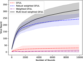
(a) $C=0$

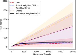
(b) $C=60$

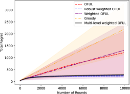
(c) $C=180$

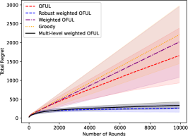
(d) $C=300$

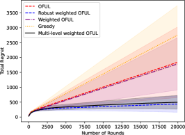
(e) $C=600$

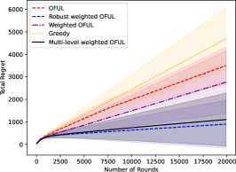
(f) $C=900$

Figure 1: Regret plot against number of rounds under corruption level from 0 to 900 averaged in 10 trials.

We plot the regret with respect to the number of rounds in Figure 1. The results are averaged over 10 trials. In the setting where $C=0$ (Figure 1(a)), we only plot the regret of OFUL, Weighted OFUL and Multi-level weighted OFUL, robust weighted OFUL and do not plot the regret of the greedy algorithm since its regret is much worse than the other four algorithms.

We have the following observations from Figure 1. For the corruption-free case $C=0$ (Figure 1(a)), our proposed Multi-level weighted OFUL behaves worse than Weighted OFUL and OFUL, which is not surprising since Multi-level weighted OFUL has additional algorithm design to deal with the corruption and it may pay additional price in regret in the absence of corruption. Weighted OFUL outperforms OFUL remarkably since it takes advantage of the information concerning the variance of noise. For the corruption case with $C\geq 180$ (Figure 1(c) to 1(f)), our Multi-level weighted OFUL outperforms other baseline algorithms by a large margin and suffers from minor additional regret compared with Robust weighted OFUL, which suggests that it can deal with the corruption successfully.

10 Conclusion and Future Work

In this paper, we have considered the linear contextual bandit problem in the presence of adversarial corruptions. We propose a Multi-level weighted OFUL algorithm, which is provably robust to the adversarial attacks.

We leave it as an open question that whether the multiplicative dependence on $C^{2}$ in the regret upper bounds can be removed without making additional assumptions in our setting.

Appendix A Proofs from Section 4

A.1 Proof of Lemma 4.1

This lemma can be proved by a direct application of Lemma B.1.

Proof.

Applying Lemma B.1, we have

$$\|\bm{\mu}_{t}-\bm{\mu}^{*}\|_{\mathbf{\Sigma}_{t}} \leq 8\sqrt{d\log\frac{(R+1)^{2}\lambda+tA^{2}}{(R+1)^{2}\lambda}\log(4t^{2}/\delta)}+4\sqrt{d}\log(4t^{2}/\delta)+C{\sqrt{d}}+\sqrt{\lambda}\|\bm{\mu}^{*}\|_{2}$$

$$\leq 8\sqrt{d\log\frac{(R+1)^{2}\lambda+tA^{2}}{(R+1)^{2}\lambda}\log(4t^{2}/\delta)}+4\sqrt{d}\log(4t^{2}/\delta)+C{\sqrt{d}}+\sqrt{\lambda}B$$

for all $t\geq 1$ with probability at least $1-\delta$. ∎

A.2 Proof of Theoreom 4.2

Proof.

Suppose $\bm{\mu}^{*}\in\mathcal{C}_{t}$ for all $t\geq 1$. Then we can bound the total regret as follows:

$$\mathbf{Regret}(T) =\mathbb{E}\left[\sum_{t=1}^{T}\left(\langle\mathbf{a}_{t}^{*},\bm{\mu}^{*}\rangle-\langle\mathbf{a}_{t},\bm{\mu}^{*}\rangle\right)\right]$$

$$\leq\mathbb{E}\left[\sum_{t=1}^{T}\min\left(2,\langle\mathbf{a}_{t},\bm{\mu}_{t}\rangle-\langle\mathbf{a}_{t},\bm{\mu}^{*}\rangle\right)\right]$$

$$\leq\mathbb{E}\left[\sum_{t=1}^{T}\min\left(2,\|\mathbf{a}_{t}\|_{\Sigma_{t}^{-1}}\alpha_{t}\right)\right]$$

$$\leq\mathbb{E}\underbrace{\left[\sum_{t=1}^{T}\min\left(2,\alpha_{T}\|\mathbf{a}_{t}\|_{\Sigma_{t}^{-1}}\right)\right]}_{I}$$ (A.1)

where the first inequality holds since $\bm{\mu}^{*}\in\mathcal{C}_{t}$ and $\mathbf{a}_{t}=\mathop{\mathrm{argmax}}_{\mathbf{a}\in\mathcal{D}_{t}}\max_{\bm{\mu}\in\mathcal{C}_{t}}\langle\mathbf{a},\bm{\mu}\rangle$, the second inequality holds due to the definition of $\mathcal{C}_{t}$ in (4.1) and the third inequality follows from the monotonicity of $\{\alpha_{t}\}$.

We split $[T]$ into two parts to bound $I$.

Let $\mathcal{I}_{1}=\{t\in[T]|\|\mathbf{a}_{t}/\overline{\sigma}_{t}\|_{\bm{\Sigma}_{t}^{-1}}>1\},\mathcal{I}_{2}=\{t\in[T]|\|\mathbf{a}_{t}/\overline{\sigma}_{t}\|_{\bm{\Sigma}_{t}^{-1}}\leq 1\}.$

We calculate

$$|\mathcal{I}_{1}| \leq\sum_{t=1}^{T}\min\left(1,\|\mathbf{a}_{t}/\overline{\sigma}_{t}\|_{\bm{\Sigma}_{t}^{-1}}^{2}\right)$$

$$\leq 2d\log\frac{(R+1)^{2}\lambda+TA^{2}}{(R+1)^{2}\lambda}$$ (A.2)

where the second inequality holds due to Lemma D.2.

$$\sum_{t\in\mathcal{I}_{2}}\min\left(2,\alpha_{T}\|\mathbf{a}_{t}\|_{\bm{\Sigma}_{t}^{-1}}\right) \leq\alpha_{T}\sum_{t\in\mathcal{I}_{2}}\|\mathbf{a}_{t}\|_{\bm{\Sigma}_{t}^{-1}}$$

$$=\alpha_{T}\sum_{t\in\mathcal{I}_{2}}\overline{\sigma}_{t}\|\mathbf{a}_{t}/\overline{\sigma}_{t}\|_{\bm{\Sigma}_{t}^{-1}}$$

$$\leq\alpha_{T}\sqrt{\sum_{t\in\mathcal{I}_{2}}\overline{\sigma}_{t}^{2}}\cdot\sqrt{\sum_{t\in\mathcal{I}_{2}}\|\mathbf{a}_{t}/\overline{\sigma}_{t}\|_{\bm{\Sigma}_{t}^{-1}}^{2}}$$

$$\leq\alpha_{T}\left(\sqrt{\sum_{t=1}^{T}\sigma_{t}^{2}}+\sqrt{R^{2}T/d}\right)\cdot\sqrt{2d\log\frac{(R+1)^{2}\lambda+TA^{2}}{(R+1)^{2}\lambda}}$$ (A.3)

where the second inequality follows from Cauchy Schwarz inequality, the third inequality holds due to the definition of $\overline{\sigma}_{t}$ and Lemma D.2.

We can further complete the proof by substituting (A.2) and (A.3) into (A.1).

∎

Appendix B Proofs of Results in Section 5

B.1 Proof of Theorem 6.1

We first prove the following lemma which is a corruption-tolerant variant of Bernstein inequality for self-normalized vector-valued martingales introduced in Zhou et al. (2020).

Lemma B.1 (Restatement of Lemma 7.1).

Let $\{\mathcal{G}_{t}\}_{t=1}^{\infty}$ be a filtration, $\{\mathbf{x}_{t},\eta_{t}\}_{t\geq 1}$ a stochastic process so that $\mathbf{x}_{t}\in\mathbb{R}^{d}$ is $\mathcal{G}_{t}$-measurable and $\eta_{t}\in\mathbb{R}$ is $\mathcal{G}_{t+1}$-measurable. Fix $R,L,\sigma,\lambda>0,\ \bm{\mu}^{*}\in\mathbb{R}^{d}$. For $t\geq 1$ let ${y}_{t}^{\text{stoch}}=\langle\mathbf{\bm{\mu}}^{*},{\mathbf{x}}_{t}\rangle+{\eta}_{t}$ and suppose that ${\eta}_{t},{\mathbf{x}}_{t}$ also satisfy

$$|{\eta}_{t}|\leq R,\mathbb{E}[{\eta}_{t}|\mathcal{G}_{t}]=0,\mathbb{E}[{\eta}_{t}^{2}|\mathcal{G}_{t}]\leq\sigma^{2},\|{\mathbf{x}}_{t}\|_{2}\leq L.$$

Suppose $\{y_{t}\}$ is a sequence such that $\sum_{i=1}^{t}|y_{i}-y_{i}^{\text{stoch}}|=C(t)$ for all $t\geq 1$. Then, for any $0<\delta<1$, with probability at least $1-\delta$ we have $\forall t>0$,

$$\|\bm{\mu}_{t}-\bm{\mu}^{*}\|_{\mathbf{Z}_{t}}\leq\beta_{t}+C(t)+\sqrt{\lambda}\|\bm{\mu}^{*}\|_{2},$$

where for $t\geq 1$, $\bm{\mu}_{t}=\mathbf{Z}_{t}^{-1}\mathbf{b}_{t}$, $\mathbf{Z}_{t}=\lambda\mathbf{I}+\sum_{i=1}^{t}{\mathbf{x}}_{i}{\mathbf{x}}_{i}^{\top}$, $\mathbf{b}_{t}=\sum_{i=1}^{t}{y}_{i}{\mathbf{x}}_{i}$, and

$$\beta_{t}=8\sigma\sqrt{d\log\frac{d\lambda+tL^{2}}{d\lambda}\log(4t^{2}/\delta)}+4R\log(4t^{2}/\delta).$$

Proof.

See Appendix C.1. ∎

Then we prove that with high probability, all the level $\ell\geq\ell^{*}$ only influenced by limited amount of corruptions as mentioned in Section 5.

Lemma B.2 (Restatement of Lemma 7.2).

Let $\text{Corruption}_{t,\ell}$ be defined in (5.1). Then we have with probability at least $1-\delta$, for all $\ell\geq\ell^{*}$, $t\geq 1$:

$$\text{Corruption}_{t,\ell}\leq\overline{C}_{\ell}=\log(2\ell^{2}/\delta)+3.$$

We denote by $\mathcal{E}_{\text{sub}}$ the event that the above inequality holds.

Proof.

The proof of this lemma is based on Lemma C.1 introduced by Lykouris et al. (2018); for details see Appendix C.2. ∎

We define the following event to further show that our candidate confidence sets with $\ell\geq\ell^{*}$ are “robust” enough, i.e. $\mathcal{C}_{t,\ell}$ contains $\bm{\mu}^{*}$ with high probability.

Definition B.3.

Let $\ell^{*}$ be defined in (5.6). We introduce the event $\mathcal{E}_{1}$ as follows.

$$\mathcal{E}_{1}:=\left\{\forall\ell\geq\ell^{*}\ \text{and}\ t\geq 1,\|\bm{\mu}^{*}-\bm{\mu}_{t}\|_{\bm{\Sigma}_{t}}\leq\beta_{t,\ell}\ \text{and}\ \|\bm{\mu}^{*}-\bm{\mu}_{t,\ell}\|_{\bm{\Sigma}_{t,\ell}}\leq\gamma_{t,\ell}\right\}.$$ (B.1)

Recall that

$$\beta_{t,\ell}=8\sqrt{d\log\frac{(R+1)^{2}\lambda+tA^{2}}{(R+1)^{2}\lambda}\log(4t^{2}/\delta)}+4\sqrt{d}\log(4t^{2}/\delta)+2^{\ell}{\sqrt{d}}+\sqrt{\lambda}B,$$ (B.2)

$$\gamma_{t,\ell}=8\sqrt{d\log\frac{(R+1)^{2}\lambda+tA^{2}}{(R+1)^{2}\lambda}\log(8t^{2}T/\delta)}+4\sqrt{d}\log(8t^{2}T/\delta)+\overline{C}_{\ell}{\sqrt{d}}+\sqrt{\lambda}B.$$ (B.3)

Lemma B.4 (Restatement of Lemma 7.4).

Let $\mathcal{E}_{1}$ be defined in (B.1). For any $0<\delta<1$, we have $\mathbb{P}(\mathcal{E}_{1})\geq 1-3\delta$.

Proof.

See Appendix C.3. ∎

Definition B.5.

For simplicity, we define $\mathbf{a}_{t,\ell}=\mathop{\mathrm{argmax}}_{\mathbf{a}\in\mathcal{D}_{t}}\max_{\bm{\mu}\in\mathcal{C}_{t,\ell}}\langle\bm{\mu},\mathbf{a}\rangle$ for each level $\ell$.

With this definition, $\mathbf{a}_{t}$ can be seen as an action vector randomly chosen from $\mathbf{a}_{t,\ell}$, $\ell\in[\ell_{\max}]$. In the following part of this section, we show how to derive the instance-independent regret upper bound using this notation.

Lemma B.6 (Restatement of Lemms 7.5).

Suppose $\mathcal{E}_{1}$ occurs. If $f(t)\leq\ell^{*}$, we have $\langle\mathbf{a}_{t}^{*}-\mathbf{a}_{t},\bm{\mu}^{*}\rangle\leq 2\beta_{t,\ell^{*}}\|\mathbf{a}_{t}\|_{\bm{\Sigma}_{t}^{-1}}+2\beta_{t,\ell^{*}}\|\mathbf{a}_{t,\ell^{*}}\|_{\bm{\Sigma}_{t}^{-1}}.$

Lemma B.7 (Restatement of Lemms 7.6).

On event $\mathcal{E}_{1}$, if $f(t)=\ell>\ell^{*}$, we have $\langle\mathbf{a}_{t}^{*}-\mathbf{a}_{t},\bm{\mu}^{*}\rangle\leq 2\gamma_{t,\ell}\|\mathbf{a}_{t}\|_{\bm{\Sigma}_{t,\ell}^{-1}}.$

Proof of Theorem 6.1.

Suppose $\mathcal{E}_{1}$ occurs. We divide regret into two parts,

$$\mathbf{Regret}(T) =\mathbb{E}\left[\sum_{t=1}^{T}\left(\langle\mathbf{a}_{t}^{*},\bm{\mu}^{*}\rangle-\langle\mathbf{a}_{t},\bm{\mu}^{*}\rangle\right)\right]$$

$$=\underbrace{\mathbb{E}\left[\sum_{t=1}^{T}\mathds{1}(f(t)\leq\ell^{*})\left(\langle\mathbf{a}_{t}^{*},\bm{\mu}^{*}\rangle-\langle\mathbf{a}_{t},\bm{\mu}^{*}\rangle\right)\right]}_{I_{1}}$$

$$\quad+\sum_{\ell=\ell^{*}+1}^{\ell_{\max}}\underbrace{\mathbb{E}\left[\sum_{t=1}^{T}\mathds{1}(f(t)=\ell)\left(\langle\mathbf{a}_{t}^{*},\bm{\mu}^{*}\rangle-\langle\mathbf{a}_{t},\bm{\mu}^{*}\rangle\right)\right]}_{I_{2}(\ell)},$$ (B.4)

where the first equality holds by definition in (3.3).

By Lemma C.3, we have

$$I_{1}\leq\mathbb{E}\left[\sum_{t=1}^{T}\mathds{1}(f(t)\leq\ell^{*})\min\left\{2,2\beta_{t,\ell^{*}}\|\mathbf{a}_{t,\ell^{*}}\|_{\bm{\Sigma}_{t}^{-1}}+2\beta_{t,\ell^{*}}\|\mathbf{a}_{t}\|_{\bm{\Sigma}_{t}^{-1}}\right\}\right].$$ (B.5)

Let $\mathcal{F}_{t}$ be the $\sigma$-algebra generated by $\mathbf{a}_{s},r_{s},\sigma_{s},f(s)$ for $s\leq t-1$. Note that

$$\mathbb{E}\left[\mathds{1}(f(t)\leq\ell^{*})\|\mathbf{a}_{t,\ell^{*}}\|_{\bm{\Sigma}_{t}^{-1}}|\mathcal{F}_{t}\right] =\mathbb{P}(f(t)\leq\ell^{*})\|\mathbf{a}_{t,\ell^{*}}\|_{\bm{\Sigma}_{t}^{-1}}$$

$$\leq 2^{\ell^{*}}\mathbb{P}(f(t)=\ell^{*})\|\mathbf{a}_{t,\ell^{*}}\|_{\bm{\Sigma}_{t}^{-1}}$$

$$\leq 2^{\ell^{*}}\mathbb{E}\left[\|\mathbf{a}_{t}\|_{\bm{\Sigma}_{t}^{-1}}|\mathcal{F}_{t}\right],$$ (B.6)

where the first equality holds since $\mathbf{a}_{t,\ell^{*}}$ and $\bm{\Sigma}_{t}$ is deterministic given $\mathcal{F}_{t}$, the first inequality holds since $\mathbb{P}(f(t)=\ell^{*})=2^{-\ell^{*}}$, the last inequality holds due to the fact that $\mathbb{P}(f(t)=\ell^{*})\|\mathbf{a}_{t,\ell^{*}}\|_{\bm{\Sigma}_{t}^{-1}}=\mathbb{E}\left[\mathds{1}(f(t)=\ell^{*})\|\mathbf{a}_{t}\|_{\bm{\Sigma}_{t}^{-1}}|\mathcal{F}_{t}\right].$

Substituting (B.6) into (B.5), we have

$$I_{1}\leq 2^{\ell^{*}}\mathbb{E}\left[\sum_{t=1}^{T}4\min\{\beta_{t,\ell^{*}}\|\mathbf{a}_{t}\|_{\bm{\Sigma}_{t}^{-1}},2\}\right]\leq 4\cdot 2^{\ell^{*}}\mathbb{E}\underbrace{\left[\sum_{t=1}^{T}\min\left\{2,\beta_{T,\ell^{*}}\|\mathbf{a}_{t}\|_{\bm{\Sigma}_{t}^{-1}}\right\}\right]}_{I_{3}}$$ (B.7)

We split $[T]$ into 2 parts to bound $I_{3}$.

Let $\mathcal{I}_{1}=\{t\in[T]|\|\mathbf{a}_{t}/\overline{\sigma}_{t}\|_{\bm{\Sigma}_{t}^{-1}}>1\},\mathcal{I}_{2}=\{t\in[T]|\|\mathbf{a}_{t}/\overline{\sigma}_{t}\|_{\bm{\Sigma}_{t}^{-1}}\leq 1\}.$

$$\sum_{t\in\mathcal{I}_{1}}\min\left\{2,\beta_{T,\ell^{*}}\|\mathbf{a}_{t}\|_{\bm{\Sigma}_{t}^{-1}}\right\}\leq 2|\mathcal{I}_{1}|\leq 2\sum_{t=1}^{T}\min\left\{1,\|\mathbf{a}_{t}/\overline{\sigma}_{t}\|_{\bm{\Sigma}_{t}^{-1}}^{2}\right\}\leq 4d\log\frac{(R+1)^{2}\lambda+TA^{2}}{(R+1)^{2}\lambda},$$ (B.8)

where the first inequality holds since $\min\left\{2,\beta_{T,\ell^{*}}\|\mathbf{a}_{t}\|_{\bm{\Sigma}_{t}^{-1}}\right\}\leq 2$, the second inequality follows from the definition of $\mathcal{I}_{1}$, the third inequality holds by Lemma D.2.

$$\sum_{t\in\mathcal{I}_{2}}\min\left\{2,\beta_{T,\ell^{*}}\|\mathbf{a}_{t}\|_{\bm{\Sigma}_{t}^{-1}}\right\} \leq\beta_{T,\ell^{*}}\sqrt{\sum_{t\in\mathcal{I}_{2}}\overline{\sigma}_{t}^{2}}\cdot\sqrt{\sum_{t\in\mathcal{I}_{2}}\min\left\{1,\|\mathbf{a}_{t}/\overline{\sigma}_{t}\|_{\bm{\Sigma}_{t}^{-1}}^{2}\right\}}$$

$$\leq\beta_{T,\ell^{*}}\sqrt{(R+1)^{2}T/d+\sum_{t=1}^{T}{\sigma}_{t}^{2}}\cdot\sqrt{2d\log\frac{(R+1)^{2}\lambda+TA^{2}}{(R+1)^{2}\lambda}},$$ (B.9)

where the first inequality follows from Cauchy-Schwarz inequality, the second inequality follows from the definition of $\overline{\sigma}_{t}$ and Lemma D.2.

Substituting (B.8) and (B.9) into (B.7), we have

$$I_{1}=\widetilde{O}\left(C^{2}d\sqrt{\sum_{t=1}^{T}\sigma_{t}^{2}}+C^{2}R\sqrt{dT}\right).$$ (B.10)

By Lemma C.4,

$$I_{2}(\ell) \leq\mathbb{E}\left[\sum_{t=1}^{T}\mathds{1}(f(t)=\ell)\min\left\{2,2\gamma_{t,\ell}\|\mathbf{a}_{t,\ell}\|_{\bm{\Sigma}_{t,\ell}^{-1}}\right\}\right]$$

$$\leq 2\mathbb{E}\underbrace{\left[\sum_{t=1}^{T}\mathds{1}(f(t)=\ell)\min\left\{1,\gamma_{t,\ell}\|\mathbf{a}_{t,\ell}\|_{\bm{\Sigma}_{t,\ell}^{-1}}\right\}\right]}_{I_{4}}$$ (B.11)

Again, we divide $[T]$ into two parts. Let $\mathcal{J}_{1}=\{t\in[T]|\|\mathbf{a}_{t,\ell}/\overline{\sigma}_{t}\|_{\bm{\Sigma}_{t,\ell}^{-1}}>1\},\mathcal{J}_{2}=\{t\in[T]|\|\mathbf{a}_{t,\ell}/\overline{\sigma}_{t}\|_{\bm{\Sigma}_{t,\ell}^{-1}}\leq 1\}.$

$$\sum_{t\in\mathcal{J}_{1}}\mathds{1}(f(t)=\ell)\min\left\{1,\gamma_{t,\ell}\|\mathbf{a}_{t,\ell}\|_{\bm{\Sigma}_{t,\ell}^{-1}}\right\} \leq\sum_{t\in\mathcal{J}_{1}}\mathds{1}(f(t)=\ell)\cdot 1$$

$$\leq\sum_{t=1}^{T}\mathds{1}(f(t)=\ell)\min\left\{1,\|\mathbf{a}_{t,\ell}\|_{\bm{\Sigma}_{t,\ell}^{-1}}^{2}\right\}$$

$$\leq 2d\log\frac{(R+1)^{2}\lambda+TA^{2}}{(R+1)^{2}\lambda},$$ (B.12)

where the second inequality follows from the definition of $\mathcal{J}_{1}$, the second inequality holds due to Lemma D.2.

$$\sum_{t\in\mathcal{J}_{2}}\mathds{1}(f(t)=\ell)\min\left\{1,\gamma_{t,\ell}\|\mathbf{a}_{t,\ell}\|_{\bm{\Sigma}_{t,\ell}^{-1}}\right\}$$

$$\leq\gamma_{T,\ell}\sqrt{\sum_{t=1}^{T}\overline{\sigma}_{t}^{2}}\sqrt{\sum_{t\in\mathcal{J}_{2}}\min\left\{1,\|\mathbf{a}_{t}/\overline{\sigma}_{t}\|_{\bm{\Sigma}_{t,\ell}^{-1}}^{2}\right\}}$$

$$\leq\gamma_{T,\ell}\sqrt{(R+1)^{2}T/d+\sum_{t=1}^{T}\sigma_{t}^{2}}\sqrt{2d\log\frac{(R+1)^{2}\lambda+TA^{2}}{(R+1)^{2}\lambda}},$$ (B.13)

where the first inequality follows from Cauchy-Schwarz inequality, the second inequality follows from the definition of $\overline{\sigma}_{t}$ and Lemma D.2.

Substituting (B.12) and (B.13) into (B.11), we have

$$I_{2}(\ell)\leq 4d\log\frac{(R+1)^{2}\lambda+TA^{2}}{(R+1)^{2}\lambda}+2\gamma_{T,\ell}\sqrt{(R+1)^{2}T/d+\sum_{t=1}^{T}\sigma_{t}^{2}}\sqrt{2d\log\frac{(R+1)^{2}\lambda+TA^{2}}{(R+1)^{2}\lambda}}$$ (B.14)

$$I_{2}(\ell)=\widetilde{O}\left(R\sqrt{Td}+d\sqrt{\sum_{t=1}^{T}\sigma_{t}^{2}}\right).$$ (B.15)

Substituting (B.10) and (B.15) into (B.4), we have

$$\mathbf{Regret}(T)=\widetilde{O}\left(C^{2}d\sqrt{\sum_{t=1}^{T}\sigma_{t}^{2}}+C^{2}R\sqrt{dT}\right).$$

∎

B.2 Proof of Theorem 6.6

Proof of Theorem 6.6.

First we decompose the regret as follows.

$$\mathbf{Regret}(T) =\mathbb{E}\left[\sum_{t=1}^{T}\left(\langle\mathbf{a}_{t}^{*},\bm{\mu}^{*}\rangle-\langle\mathbf{a}_{t},\bm{\mu}^{*}\rangle\right)\right]$$

$$\leq\frac{1}{{\Delta}}\underbrace{\mathbb{E}\left[\sum_{t=1}^{T}\mathds{1}(f(t)\leq\ell^{*})\left(\langle\mathbf{a}_{t}^{*},\bm{\mu}^{*}\rangle-\langle\mathbf{a}_{t},\bm{\mu}^{*}\rangle\right)^{2}\right]}_{I_{1}}$$

$$\qquad+\sum_{\ell=\ell^{*}+1}^{\ell_{\max}}\frac{1}{{\Delta}}\underbrace{\mathbb{E}\left[\sum_{t=1}^{T}\mathds{1}(f(t)=\ell)\left(\langle\mathbf{a}_{t}^{*},\bm{\mu}^{*}\rangle-\langle\mathbf{a}_{t},\bm{\mu}^{*}\rangle\right)^{2}\right]}_{I_{2}(\ell)},$$ (B.16)

where the first equality holds due to the definition in (3.3), the last inequality follows from the fact that either $\langle\mathbf{a}_{t}^{*},\bm{\mu}^{*}\rangle-\langle\mathbf{a}_{t},\bm{\mu}^{*}\rangle=0$ or $\overline{\Delta}_{T}\leq\langle\mathbf{a}_{t}^{*},\bm{\mu}^{*}\rangle-\langle\mathbf{a}_{t},\bm{\mu}^{*}\rangle$. To bound $I_{1}$, we have

$$I_{1} \leq\mathbb{E}\left[\sum_{t=1}^{T}\mathds{1}(f(t)\leq\ell^{*})\min\left\{4,\left(2\beta_{t,\ell^{*}}\|\mathbf{a}_{t,\ell^{*}}\|_{\bm{\Sigma}_{t}^{-1}}+2\beta_{t,\ell^{*}}\|\mathbf{a}_{t}\|_{\bm{\Sigma}_{t}^{-1}}\right)^{2}\right\}\right]$$

$$\leq 2^{\ell^{*}}\mathbb{E}\underbrace{\left[\sum_{t=1}^{T}\min\left\{4,16\beta_{t,\ell^{*}}^{2}\|\mathbf{a}_{t}\|_{\bm{\Sigma}_{t}^{-1}}^{2}\right\}\right]}_{I_{3}},$$ (B.17)

where the first inequality holds due to Lemma B.6 and the second inequality follows from a similar argument as (B.6). To further bound $I_{3}$, we decompose $[T]$ into two non-overlapping sets: $\mathcal{I}_{1}=\{t\in[T]|\|\mathbf{a}_{t}/\overline{\sigma}_{t}\|_{\bm{\Sigma}_{t}^{-1}}>1\},\mathcal{I}_{2}=\{t\in[T]|\|\mathbf{a}_{t}/\overline{\sigma}_{t}\|_{\bm{\Sigma}_{t}^{-1}}\leq 1\}$. For $\mathcal{I}_{1}$, we have

$$\sum_{t\in\mathcal{I}_{1}}\min\left\{4,16\beta_{t,\ell^{*}}^{2}\|\mathbf{a}_{t}\|_{\bm{\Sigma}_{t}^{-1}}^{2}\right\} \leq 4|\mathcal{I}_{1}|$$

$$\leq 4\sum_{t=1}^{T}\min\left\{1,\|\mathbf{a}_{t}/\overline{\sigma_{t}}\|_{\bm{\Sigma}_{t}^{-1}}^{2}\right\}$$

$$\leq 8d\log\frac{(R+1)^{2}\lambda+TA^{2}}{(R+1)^{2}\lambda},$$ (B.18)

where the third inequality holds due to Lemma D.2. For $\mathcal{I}_{2}$, we have

$$\sum_{t\in\mathcal{I}_{2}}\min\left\{4,9\beta_{t,\ell^{*}}^{2}\|\mathbf{a}_{t}\|_{\bm{\Sigma}_{t}^{-1}}^{2}\right\} \leq 16\beta_{T,\ell^{*}}^{2}\max_{t\in[T]}\overline{\sigma}_{t}^{2}\sum_{t\in\mathcal{I}_{2}}\min\left\{1,\|\mathbf{a}_{t}/\overline{\sigma_{t}}\|_{\bm{\Sigma}_{t}^{-1}}^{2}\right\}$$

$$\leq 32\beta_{T,\ell^{*}}^{2}(\max_{t\in[T]}{\sigma}_{t}^{2}+(R+1)^{2}/d)d\log\frac{(R+1)^{2}\lambda+TA^{2}}{(R+1)^{2}\lambda},$$ (B.19)

where the first inequality follows from the definition of $\mathcal{I}_{2}$, the second inequality follows from Lemma D.2.

Substituting (B.18) and (B.19) into (B.17), we have

$$I_{1}=\widetilde{O}\left(C^{2}R^{2}d+d^{2}C^{2}\max_{t\in[T]}\sigma_{t}^{2}\right).$$ (B.20)

To bound $I_{2}(\ell)$, by Lemma B.7, we have

$$I_{2}(\ell) \leq\mathbb{E}\left[\sum_{t=1}^{T}\mathds{1}(f(t)=\ell)\min\left\{4,4\gamma_{t,\ell}^{2}\|\mathbf{a}_{t}\|_{\bm{\Sigma}_{t,\ell}^{-1}}^{2}\right\}\right]$$

$$\leq 4\mathbb{E}\underbrace{\left[\sum_{t=1}^{T}\mathds{1}(f(t)=\ell)\min\left\{1,\gamma_{t,\ell}^{2}\|\mathbf{a}_{t}\|_{\bm{\Sigma}_{t,\ell}^{-1}}^{2}\right\}\right]}_{I_{4}}.$$ (B.21)

We divide $[T]$ into two parts to calculate $I_{4}$. Let $\mathcal{J}_{1}=\{t\in[T]|\|\mathbf{a}_{t}/\overline{\sigma}_{t}\|_{\bm{\Sigma}_{t,\ell}^{-1}}>1\},\mathcal{J}_{2}=\{t\in[T]|\|\mathbf{a}_{t}/\overline{\sigma}_{t}\|_{\bm{\Sigma}_{t,\ell}^{-1}}\leq 1\}.$ For $\mathcal{J}_{1}$, we have

$$\sum_{t\in\mathcal{J}_{1}}\mathds{1}(f(t)=\ell)\min\left\{1,\gamma_{t,\ell}^{2}\|\mathbf{a}_{t}\|_{\bm{\Sigma}_{t,\ell}^{-1}}^{2}\right\} \leq|\mathcal{J}_{1}|$$

$$\leq\sum_{t\in[T]}\min\left\{1,\|\mathbf{a}_{t}\|_{\bm{\Sigma}_{t,\ell}^{-1}}^{2}\right\}$$

$$\leq 2d\log\frac{(R+1)^{2}\lambda+TA^{2}}{(R+1)^{2}\lambda},$$ (B.22)

where the second inequality follows from the fact that $\mathcal{J}_{1}\subseteq[T]$, the third inequality holds due to Lemma D.2. For $\mathcal{J}_{2}$, we have

$$\sum_{t\in\mathcal{J}_{2}}\mathds{1}(f(t)=\ell)\min\left\{1,\gamma_{t,\ell}^{2}\|\mathbf{a}_{t}\|_{\bm{\Sigma}_{t,\ell}^{-1}}^{2}\right\} \leq\gamma_{T,\ell}^{2}\max_{t\in[T]}\overline{\sigma}_{t}^{2}\sum_{t\in\mathcal{J}_{2}}\|\mathbf{a}_{t}\|_{\bm{\Sigma}_{t,\ell}^{-1}}^{2}$$

$$\leq\gamma_{T,\ell}^{2}(\max_{t\in[T]}{\sigma}_{t}^{2}+(R+1)^{2}/d)\sum_{t\in[T]}\min\left\{1,\|\mathbf{a}\|_{\bm{\Sigma}_{t,\ell}^{-1}}^{2}\right\}$$

$$\leq\gamma_{T,\ell}^{2}(\max_{t\in[T]}{\sigma}_{t}^{2}+(R+1)^{2}/d)2d\log\frac{(R+1)^{2}\lambda+TA^{2}}{(R+1)^{2}\lambda},$$ (B.23)

where the second inequality follows from the definition of $\overline{\sigma}_{t}$ and $\mathcal{J}_{2}$ and the third inequality holds due to Lemma D.2.

Substituting (B.22) and (B.23) into (B.21), we have

$$I_{2}(\ell)=\widetilde{O}(dR^{2}+d^{2}\max_{t\in[T]}\sigma_{t}^{2}).$$ (B.24)

Finally, substituting (B.24) and (B.20) into (B.16), we have

$$\mathbf{Regret}(T)=\frac{1}{\Delta}\widetilde{O}\left(C^{2}R^{2}d+d^{2}C^{2}\max_{t\in[T]}\sigma_{t}^{2}\right).$$

∎

Appendix C Proof of Technical Lemmas in Appendix B

C.1 Proof of Lemma B.1

Proof.

Let ${\mathcal{S}}(t)=\{1\leq i\leq t|y_{i}\neq y_{i}^{\text{stoch}}\}$, $\mathbf{b}_{t}^{\text{stoch}}=\sum_{i=1}^{t}y_{i}^{\text{stoch}}\mathbf{x}_{i}$ and $\bm{\mu}_{t}^{\text{stoch}}=\mathbf{Z}_{t}^{-1}\mathbf{b}_{t}^{\text{stoch}}$. By Lemma D.1, we have that with probability at least $1-\delta$, $\|\bm{\mu}_{t}^{\text{stoch}}-\bm{\mu}^{*}\|_{\mathbf{Z}_{t}}\leq\beta_{t}+\sqrt{\lambda}\|\bm{\mu}^{*}\|_{2}$ holds for all $t\geq 1$.

Also, we have

$$\|\bm{\mu}_{t}-\bm{\mu}_{t}^{\text{stoch}}\|_{\mathbf{Z}_{t}} =\|\mathbf{Z}_{t}^{-1}(\mathbf{b}_{t}-\mathbf{b}_{t}^{\text{stoch}})\|_{\mathbf{Z}_{t}}$$

$$\leq\sum_{i=1}^{t}\|\mathbf{Z}_{t}^{-1}(y_{i}^{\text{stoch}}-y_{i})\mathbf{x}_{i}\|_{\mathbf{Z}_{t}}$$

$$\leq\sum_{i=1}^{t}|y_{i}^{\text{stoch}}-y_{i}|\cdot\|\mathbf{x}_{i}\|_{\mathbf{Z}_{t}^{-1}}$$

$$\leq C(t).$$

where the first inequality holds due to the triangle inequality and the last inequality holds due to $\|\mathbf{x}_{i}\|_{\mathbf{Z}_{t}^{-1}}\leq 1$.

Hence, we can obtain

$$\|\bm{\mu}_{t}-\bm{\mu}^{*}\|_{\mathbf{Z}_{t}}\leq\|\bm{\mu}_{t}^{\text{stoch}}-\bm{\mu}^{*}\|_{\mathbf{Z}_{t}}+\|\bm{\mu}_{t}-\bm{\mu}_{t}^{\text{stoch}}\|_{\mathbf{Z}_{t}}\leq\beta_{t}+C(t)+\sqrt{\lambda}\|\bm{\mu}^{*}\|_{2}.$$

∎

C.2 Proof of Lemma B.2

Lemma C.1 (Lemma 3.3, Lykouris et al. 2018).

Define the corruption level for a level $\ell$:

$$\text{Corruption}_{t,\ell}=\sum_{i=1}^{t}\frac{\mathds{1}(f(i)=\ell)}{R+1}\cdot\sup_{\mathbf{a}\in\mathcal{D}_{i}}\left|r_{i}(\mathbf{a})-r_{i}^{\prime}(\mathbf{a})\right|.$$

Then we have for all $\ell\geq\ell^{*}$, with probability at least $1-\delta$:

$$\text{Corruption}_{t,\ell}\leq\log(1/\delta)+3,\qquad\forall t\geq 1.$$

Proof of Lemma B.2.

Applying Lemma C.1, we have for all $\ell\geq\ell^{*}$, with probability at least $1-\delta/(2\ell^{2})$: $\text{Corruption}_{t,\ell}\leq\log(2\ell^{2}/\delta)+3,\forall t\geq 1.$

Using a union bound over all $\ell\geq\ell^{*}$, we can prove the lemma. ∎

C.3 Proof of Lemma B.4

To prove the lemma, we first define the following two events:

$$\mathcal{E}_{2} :=\left\{\forall\ell\geq\ell^{*}\ \text{and}\ t\geq 1,\|\bm{\mu}^{*}-\bm{\mu}_{t}\|_{\bm{\Sigma}_{t}}\leq\beta_{t,\ell}\right\}$$ (C.1)

$$\mathcal{E}_{3} :=\left\{\forall\ell\geq\ell^{*}\ \text{and}\ t\geq 1,\|\bm{\mu}^{*}-\bm{\mu}_{t,\ell}\|_{\bm{\Sigma}_{t,\ell}}\leq\gamma_{t,\ell}\right\}$$ (C.2)

Lemma C.2.

Let $\mathcal{E}_{2}$ be defined in (C.1). For any $0<\delta<1$, we have $\mathbb{P}(\mathcal{E}_{2})\geq 1-\delta$.

Proof.

Applying Lemma B.1, we have that

$$\|\bm{\mu}_{t}-\bm{\mu}^{*}\|_{\mathbf{\Sigma}_{t}}\leq 8\sqrt{d\log\frac{(R+1)^{2}\lambda+tA^{2}}{(R+1)^{2}\lambda}\log(4t^{2}/\delta)}+4\sqrt{d}\log(4t^{2}/\delta)+C{\sqrt{d}}+\sqrt{\lambda}\|\bm{\mu}^{*}\|_{2}$$

for all $t\geq 1$ with probability at least $1-\delta$. Note that $2^{\ell}\geq C$ for all $\ell\geq\ell^{*}$, which indicates that $\mathcal{E}_{2}$ occurs with probability at least $1-\delta$. ∎

Lemma C.3.

Let $\mathcal{E}_{3}$ be defined in (C.2). For any $0<\delta<1$, we have $\mathbb{P}(\mathcal{E}_{3})\geq 1-2\delta$.

Proof.

Applying Lemma B.1, we have that $\|\bm{\mu}_{t,\ell}-\bm{\mu}^{*}\|_{\mathbf{\Sigma}_{t}}\leq 8\sqrt{d\log\frac{(R+1)^{2}\lambda+tA^{2}}{(R+1)^{2}\lambda}\log(4t^{2}T/\delta)}+4\sqrt{d}\log(4t^{2}T/\delta)+\text{Corruption}_{t,\ell}{\sqrt{d}}+\sqrt{\lambda}\|\bm{\mu}^{*}\|_{2}$ for all $t\geq 1$ with probability at least $1-\delta/\ell$. Here we use the fact that $\ell\leq T$. Applying Lemma B.2 and a union bound, we have $\mathcal{E}_{3}$ occurs with probability at least $1-2\delta$. ∎

Proof of Lemma B.4.

This lemma can be proved by a union bound on $\mathcal{E}_{2}$ and $\mathcal{E}_{3}$ with Lemmas C.2 and C.3. ∎

C.4 Proof of Lemma B.6

Proof.

For simplicity, let $\mathcal{A}_{t,\ell}=\left\{\bm{\mu}|\|\bm{\mu}-\bm{\mu}_{t}\|_{\bm{\Sigma}_{t}}\leq\beta_{t,\ell}\right\},\mathcal{B}_{t,\ell}=\left\{\bm{\mu}|\|\bm{\mu}-\bm{\mu}_{t,\ell}\|_{\bm{\Sigma}_{t,\ell}}\leq\gamma_{t,\ell}\right\}.$ Let $\bm{\mu}_{t}^{m}=\mathop{\mathrm{argmax}}_{\bm{\mu}\in\mathcal{C}_{t,f(t)}}\langle\mathbf{a}_{t},\bm{\mu}\rangle.$ Then we have

$$\langle\mathbf{a}_{t},\bm{\mu}^{*}\rangle \geq\langle\mathbf{a}_{t},\bm{\mu}_{t}\rangle-\beta_{t,\ell^{*}}\|\mathbf{a}_{t}\|_{\bm{\Sigma}_{t}^{-1}}$$

$$\geq\langle\mathbf{a}_{t},\bm{\mu}_{t}^{m}\rangle-2\beta_{t,\ell^{*}}\|\mathbf{a}_{t}\|_{\bm{\Sigma}_{t}^{-1}}$$

$$\geq\langle\mathbf{a}_{t,\ell^{*}},\bm{\mu}_{t}^{m}\rangle-2\beta_{t,\ell^{*}}\|\mathbf{a}_{t}\|_{\bm{\Sigma}_{t}^{-1}}$$

$$\geq\langle\mathbf{a}_{t,\ell^{*}},\bm{\mu}_{t}\rangle-\beta_{t,\ell^{*}}\|\mathbf{a}_{t,\ell^{*}}\|_{\bm{\Sigma}_{t}^{-1}}-2\beta_{t,\ell^{*}}\|\mathbf{a}_{t}\|_{\bm{\Sigma}_{t}^{-1}}$$

$$\geq\max_{\bm{\mu}\in\mathcal{A}_{t,\ell^{*}}}\langle\mathbf{a}_{t,\ell^{*}},\bm{\mu}\rangle-2\beta_{t,\ell^{*}}\|\mathbf{a}_{t,\ell^{*}}\|_{\bm{\Sigma}_{t}^{-1}}-2\beta_{t,\ell^{*}}\|\mathbf{a}_{t}\|_{\bm{\Sigma}_{t}^{-1}},$$

$$\geq\max_{\bm{\mu}\in\mathcal{C}_{t,\ell^{*}}}\langle\mathbf{a}_{t,\ell^{*}},\bm{\mu}\rangle-2\beta_{t,\ell^{*}}\|\mathbf{a}_{t,\ell^{*}}\|_{\bm{\Sigma}_{t}^{-1}}-2\beta_{t,\ell^{*}}\|\mathbf{a}_{t}\|_{\bm{\Sigma}_{t}^{-1}},$$ (C.3)

where the first inequality holds since $\bm{\mu}^{*}\in\mathcal{C}_{t,\ell^{*}}\subseteq\mathcal{A}_{t,l^{*}}$, the second inequality holds since $\bm{\mu}_{t}^{m}\in\mathcal{C}_{t,f(t)}\subseteq\mathcal{A}_{t,l^{*}}$, the third inequality holds by the definition of $\mathbf{a}_{t}$ and $\bm{\mu}_{t}^{m}$, the fourth inequality holds since $\bm{\mu}_{t}^{m}\in\mathcal{A}_{t,\ell^{*}}$, the fifth inequality holds since $\bm{\mu}_{t}\in\mathcal{A}_{t,\ell^{*}}$, the last one holds since $\mathcal{C}_{t,\ell^{*}}\subseteq\mathcal{A}_{t,\ell^{*}}$. By the definition of $\mathcal{E}_{1}$ and $\mathbf{a}_{t,\ell^{*}}$, we have

$$\max_{\bm{\mu}\in\mathcal{C}_{t,\ell^{*}}}\langle\mathbf{a}_{t,\ell^{*}},\bm{\mu}\rangle=\max_{\mathbf{a}\in\mathcal{D}_{t}}\max_{\bm{\mu}\in\mathcal{C}_{t,\ell^{*}}}\langle\mathbf{a},\bm{\mu}\rangle\geq\max_{\mathbf{a}\in\mathcal{D}_{t}}\langle\mathbf{a},\bm{\mu}^{*}\rangle=\langle\mathbf{a}_{t}^{*},\bm{\mu}^{*}\rangle.$$ (C.4)

Combining (C.3) with (C.4), we have $\langle\mathbf{a}_{t}^{*}-\mathbf{a}_{t},\bm{\mu}^{*}\rangle\leq 2\beta_{t,\ell^{*}}\|\mathbf{a}_{t}\|_{\bm{\Sigma}_{t}^{-1}}+2\beta_{t,\ell^{*}}\|\mathbf{a}_{t,\ell^{*}}\|_{\bm{\Sigma}_{t}^{-1}}.$ ∎

C.5 Proof of Lemma B.7

Proof.

We have

$$\langle\mathbf{a}_{t}^{*}-\mathbf{a}_{t},\bm{\mu}^{*}\rangle \leq\max_{\bm{\mu}\in\mathcal{C}_{t,\ell}}\langle\mathbf{a}_{t},\bm{\mu}\rangle-\langle\mathbf{a}_{t},\bm{\mu}^{*}\rangle\leq 2\gamma_{t,\ell}\|\mathbf{a}_{t}\|_{\bm{\Sigma}_{t,\ell}^{-1}},$$

where the first inequality follows from the fact that $\bm{\mu}^{*}\in\mathcal{C}_{t,\ell}$ and the definition of $\mathbf{a}_{t}$, the second inequality holds since $\bm{\mu}^{*}\in\mathcal{C}_{t,\ell}$ on the event $\mathcal{E}_{1}$. ∎

Appendix D Auxiliary Lemmas

Lemma D.1 (Theorem 4.1, Zhou et al. 2020).

Let $\{\mathcal{G}_{t}\}_{t=1}^{\infty}$ be a filtration, $\{\mathbf{x}_{t},\eta_{t}\}_{t\geq 1}$ a stochastic process so that $\mathbf{x}_{t}\in\mathbb{R}^{d}$ is $\mathcal{G}_{t}$-measurable and $\eta_{t}\in\mathbb{R}$ is $\mathcal{G}_{t+1}$-measurable. Fix $R,L,\sigma,\lambda>0,\ \bm{\mu}^{*}\in\mathbb{R}^{d}$. For $t\geq 1$ let ${y}_{t}=\langle\mathbf{\bm{\mu}}^{*},{\mathbf{x}}_{t}\rangle+{\eta}_{t}$ and suppose that ${\eta}_{t},{\mathbf{x}}_{t}$ also satisfy

$$|{\eta}_{t}|\leq R,\mathbb{E}[{\eta}_{t}|\mathcal{G}_{t}]=0,\mathbb{E}[{\eta}_{t}^{2}|\mathcal{G}_{t}]\leq\sigma^{2},\|{\mathbf{x}}_{t}\|_{2}\leq L.$$

Then, for any $0<\delta<1$, with probability at least $1-\delta$ we have $\forall t>0$,

$$\|\bm{\mu}_{t}-\bm{\mu}^{*}\|_{\mathbf{Z}_{t}}\leq\beta_{t}+\sqrt{\lambda}\|\bm{\mu}^{*}\|_{2},$$

where for $t\geq 1$, $\bm{\mu}_{t}=\mathbf{Z}_{t}^{-1}\mathbf{b}_{t}$, $\mathbf{Z}_{t}=\lambda\mathbf{I}+\sum_{i=1}^{t}{\mathbf{x}}_{i}{\mathbf{x}}_{i}^{\top}$, $\mathbf{b}_{t}=\sum_{i=1}^{t}{y}_{i}{\mathbf{x}}_{i}$, and

$$\beta_{t}=8\sigma\sqrt{d\log\frac{d\lambda+tL^{2}}{d\lambda}\log(4t^{2}/\delta)}+4R\log(4t^{2}/\delta).$$

Lemma D.2 (Lemma 11, Abbasi-Yadkori et al. 2011).

For any $\lambda>0$ and sequence $\{\mathbf{x}_{t}\}_{t=1}^{T}\subset\mathbb{R}^{d}$ for $t\in 0\cup[T]$, define $\mathbf{Z}_{t}=\lambda\mathbf{I}+\sum_{i=1}^{t}\mathbf{x}_{i}\mathbf{x}_{i}^{\top}$. Then, provided that $\|\mathbf{x}_{t}\|_{2}\leq L$ holds for all $t\in[T]$, we have

$$\sum_{t=1}^{T}\min\{1,\|\mathbf{x}_{t}\|_{\mathbf{Z}_{t-1}^{-1}}^{2}\}\leq 2d\log\frac{d\lambda+TL^{2}}{d\lambda}.$$

References

- Abbasi-Yadkori et al. (2011) Abbasi-Yadkori, Y., Pál, D. and Szepesvári, C. (2011). Improved algorithms for linear stochastic bandits. In NIPS, vol. 11.
- Abe et al. (2003) Abe, N., Biermann, A. W. and Long, P. M. (2003). Reinforcement learning with immediate rewards and linear hypotheses. Algorithmica 37 263–293.
- Agarwal et al. (2017) Agarwal, A., Luo, H., Neyshabur, B. and Schapire, R. E. (2017). Corralling a band of bandit algorithms. In Conference on Learning Theory. PMLR.
- Auer (2002) Auer, P. (2002). Using confidence bounds for exploitation-exploration trade-offs. Journal of Machine Learning Research 3 397–422.
- Auer et al. (2002) Auer, P., Cesa-Bianchi, N., Freund, Y. and Schapire, R. E. (2002). The nonstochastic multiarmed bandit problem. SIAM journal on computing 32 48–77.
- Auer and Chiang (2016) Auer, P. and Chiang, C.-K. (2016). An algorithm with nearly optimal pseudo-regret for both stochastic and adversarial bandits. In Conference on Learning Theory. PMLR.
- Bogunovic et al. (2021) Bogunovic, I., Losalka, A., Krause, A. and Scarlett, J. (2021). Stochastic linear bandits robust to adversarial attacks. In International Conference on Artificial Intelligence and Statistics. PMLR.
- Bubeck and Cesa-Bianchi (2012) Bubeck, S. and Cesa-Bianchi, N. (2012). Regret analysis of stochastic and nonstochastic multi-armed bandit problems. arXiv preprint arXiv:1204.5721 .
- Bubeck and Slivkins (2012) Bubeck, S. and Slivkins, A. (2012). The best of both worlds: Stochastic and adversarial bandits. In Conference on Learning Theory. JMLR Workshop and Conference Proceedings.
- Cheung et al. (2019) Cheung, W. C., Simchi-Levi, D. and Zhu, R. (2019). Learning to optimize under non-stationarity. In The 22nd International Conference on Artificial Intelligence and Statistics. PMLR.
- Chu et al. (2011) Chu, W., Li, L., Reyzin, L. and Schapire, R. (2011). Contextual bandits with linear payoff functions. In Proceedings of the Fourteenth International Conference on Artificial Intelligence and Statistics. JMLR Workshop and Conference Proceedings.
- Dani et al. (2008) Dani, V., Hayes, T. P. and Kakade, S. (2008). Stochastic linear optimization under bandit feedback. In COLT.
- Deshpande and Montanari (2012) Deshpande, Y. and Montanari, A. (2012). Linear bandits in high dimension and recommendation systems. In 2012 50th Annual Allerton Conference on Communication, Control, and Computing (Allerton). IEEE.
- Ding et al. (2021) Ding, Q., Hsieh, C.-J. and Sharpnack, J. (2021). Robust stochastic linear contextual bandits under adversarial attacks. arXiv preprint arXiv:2106.02978 .
- Foster et al. (2021) Foster, D. J., Gentile, C., Mohri, M. and Zimmert, J. (2021). Adapting to misspecification in contextual bandits. arXiv preprint arXiv:2107.05745 .
- Foster et al. (2019) Foster, D. J., Krishnamurthy, A. and Luo, H. (2019). Model selection for contextual bandits. arXiv preprint arXiv:1906.00531 .
- Garcelon et al. (2020) Garcelon, E., Roziere, B., Meunier, L., Tarbouriech, J., Teytaud, O., Lazaric, A. and Pirotta, M. (2020). Adversarial attacks on linear contextual bandits. arXiv preprint arXiv:2002.03839 .
- Gupta et al. (2019) Gupta, A., Koren, T. and Talwar, K. (2019). Better algorithms for stochastic bandits with adversarial corruptions. In Conference on Learning Theory. PMLR.
- Jhalani et al. (2016) Jhalani, T., Kant, V. and Dwivedi, P. (2016). A linear regression approach to multi-criteria recommender system. In International Conference on Data Mining and Big Data. Springer.
- Jun et al. (2018) Jun, K.-S., Li, L., Ma, Y. and Zhu, X. J. (2018). Adversarial attacks on stochastic bandits. In NeurIPS.
- Kannan et al. (2018) Kannan, S., Morgenstern, J. H., Roth, A., Waggoner, B. and Wu, Z. (2018). A smoothed analysis of the greedy algorithm for the linear contextual bandit problem. In NeurIPS.
- Kapoor et al. (2019) Kapoor, S., Patel, K. K. and Kar, P. (2019). Corruption-tolerant bandit learning. Machine Learning 108 687–715.
- Kirschner and Krause (2018) Kirschner, J. and Krause, A. (2018). Information directed sampling and bandits with heteroscedastic noise. In Conference On Learning Theory. PMLR.
- Lee et al. (2021) Lee, C.-W., Luo, H., Wei, C.-Y., Zhang, M. and Zhang, X. (2021). Achieving near instance-optimality and minimax-optimality in stochastic and adversarial linear bandits simultaneously. arXiv preprint arXiv:2102.05858 .
- Li et al. (2010) Li, L., Chu, W., Langford, J. and Schapire, R. E. (2010). A contextual-bandit approach to personalized news article recommendation. In Proceedings of the 19th international conference on World wide web.
- Li et al. (2019a) Li, Y., Lou, E. Y. and Shan, L. (2019a). Stochastic linear optimization with adversarial corruption. arXiv preprint arXiv:1909.02109 .
- Li et al. (2019b) Li, Y., Wang, Y. and Zhou, Y. (2019b). Nearly minimax-optimal regret for linearly parameterized bandits. In Conference on Learning Theory. PMLR.
- Liu and Shroff (2019) Liu, F. and Shroff, N. (2019). Data poisoning attacks on stochastic bandits. In International Conference on Machine Learning. PMLR.
- Locatelli and Carpentier (2018) Locatelli, A. and Carpentier, A. (2018). Adaptivity to smoothness in x-armed bandits. In Conference on Learning Theory. PMLR.
- Lykouris et al. (2018) Lykouris, T., Mirrokni, V. and Paes Leme, R. (2018). Stochastic bandits robust to adversarial corruptions. In Proceedings of the 50th Annual ACM SIGACT Symposium on Theory of Computing.
- Neu and Olkhovskaya (2020) Neu, G. and Olkhovskaya, J. (2020). Efficient and robust algorithms for adversarial linear contextual bandits. In Conference on Learning Theory. PMLR.
- Odalric and Munos (2011) Odalric, M. and Munos, R. (2011). Adaptive bandits: Towards the best history-dependent strategy. In Proceedings of the Fourteenth International Conference on Artificial Intelligence and Statistics. JMLR Workshop and Conference Proceedings.
- Pacchiano et al. (2020) Pacchiano, A., Phan, M., Abbasi-Yadkori, Y., Rao, A., Zimmert, J., Lattimore, T. and Szepesvari, C. (2020). Model selection in contextual stochastic bandit problems. arXiv preprint arXiv:2003.01704 .
- Rusmevichientong and Tsitsiklis (2010) Rusmevichientong, P. and Tsitsiklis, J. N. (2010). Linearly parameterized bandits. Mathematics of Operations Research 35 395–411.
- Seldin and Lugosi (2017) Seldin, Y. and Lugosi, G. (2017). An improved parametrization and analysis of the exp3++ algorithm for stochastic and adversarial bandits. In Conference on Learning Theory. PMLR.
- Seldin and Slivkins (2014) Seldin, Y. and Slivkins, A. (2014). One practical algorithm for both stochastic and adversarial bandits. In International Conference on Machine Learning. PMLR.
- Villar et al. (2015) Villar, S. S., Bowden, J. and Wason, J. (2015). Multi-armed bandit models for the optimal design of clinical trials: benefits and challenges. Statistical science: a review journal of the Institute of Mathematical Statistics 30 199.
- Zhou et al. (2020) Zhou, D., Gu, Q. and Szepesvari, C. (2020). Nearly minimax optimal reinforcement learning for linear mixture markov decision processes. arXiv preprint arXiv:2012.08507 .
- Zimmert and Seldin (2019) Zimmert, J. and Seldin, Y. (2019). An optimal algorithm for stochastic and adversarial bandits. In The 22nd International Conference on Artificial Intelligence and Statistics. PMLR.