MUSE: Feature Self-Distillation with Mutual Information and Self-Information

Abstract

We present a novel information-theoretic approach to introduce dependency among features of a deep convolutional neural network (CNN). The core idea of our proposed method, called MUSE, is to combine MUtual information and SElf-information to jointly improve the expressivity of all features extracted from different layers in a CNN. We present two variants of the realization of MUSE—Additive Information and Multiplicative Information. Importantly, we argue and empirically demonstrate that MUSE, compared to other feature discrepancy functions, is a more functional proxy to introduce dependency and effectively improve the expressivity of all features in the knowledge distillation framework. MUSE achieves superior performance over a variety of popular architectures and feature discrepancy functions for self-distillation and online distillation, and performs competitively with the state-of-the-art methods for offline distillation. MUSE is also demonstrably versatile that enables it to be easily extended to CNN-based models on tasks other than image classification such as object detection.

1 Introduction

There has been extensive research on convolutional neural networks (CNNs) for computer vision tasks. A variety of deep convolutional network architectures have emerged, whether empirically designed such as VGG [Simonyan and Zisserman(2015)], ResNet [He et al.(2016)He, Zhang, Ren, and Sun], WideResNet [Zagoruyko and Komodakis(2016)], DenseNet [Huang et al.(2017)Huang, Liu, van der Maaten, and Weinberger], ShuffleNet [Zhang et al.(2018)Zhang, Zhou, Lin, and Sun], or constructed using Neural Architecture Search such as NASNet [Zoph et al.(2018)Zoph, Vasudevan, Shlens, and Le] and the baseline network of EfficientNet [Tan and Le(2019)]. While the large number of network weights store the experience learned from the training data, the activations (or features) of the hidden layers represent the direct response from the network to the data. It is still an open problem how to fully utilize these intermediate features to advance the capacity of the models. In this work, we aim to improve the existing neural architectures by fully exploiting the features.

Based on provably effective neural estimator on mutual information [Belghazi et al.(2018)Belghazi, Baratin, Rajeshwar, Ozair, Bengio, Courville, and Hjelm], recent progress [Tschannen et al.(2020)Tschannen, Djolonga, Rubenstein, Gelly, and Lucic, Hjelm et al.(2019)Hjelm, Fedorov, Lavoie-Marchildon, Grewal, Bachman, Trischler, and Bengio] on unsupervised representation learning treat features as random variables and formulate the information of the features to learn a maximally informative representation of the data. Mutual Information (MI) is an information-theoretic measure to quantify the amount of information shared by two random variables. We posit that Self-information (SI), which quantifies the amount of information in one random variable, also plays an essential role. SI can be viewed as MI between two identical random variables, which enables us to estimate it using MI neural estimators. Instead of learning one single effective data representation, we aim to estimate and combine the MI and SI of multiple intermediate features to further boost the discriminative power of deep CNNs.

Knowledge distillation (KD) [Hinton et al.(2015)Hinton, Vinyals, and Dean] is the practice that was proposed to learn a comparably performant compact neural network from a powerful yet expensive teacher network without additional architecture modification. The core idea is to let the compact student network mimic the “soft targets” produced by the teacher network. It can be further divided into offline distillation where the teacher network is pretrained and fixed, and online distillation where the teacher and student networks are jointly trained from scratch. Unlike offline and online distillation, self-distillation (SD) does not involve multiple networks, but aims to learn by distilling its own knowledge. It is self-contained as it does not require an extra teacher with additional training overhead and removes the need for teacher model selection while focusing solely on the target model. Our work is under this category as we aim to improve the overall performance by the intermediate features in one single network. Prior work on SD usually relies on the penalty function proposed to distill knowledge between two networks. By treating the features as random variables, we propose a novel discrepancy function based on MUtual information and SElf-information, called MUSE, to better self-distill the knowledge from different features extracted within one network and improve each feature. We validate this approach on various backbone CNN networks on image classification and object detection and show its effectiveness. We summarize our contributions as follows:

• A novel feature discrepancy function MUSE with two realization variants, Additive Information and Multiplicative Information, to introduce strong dependencies among features within a CNN. We demonstrate its effectiveness in feature distillation and how self-information (SI) interacts with mutual information (MI) to improve distillation.

• Outperforming other state-of-the-art self-distillation (SD) methods when applying SD framework on image classification and object detection, indicating the ability of the proposed method to enhance the feature expressivity.

• Establishing the efficacy for model compression, where the compressed models perform competitively or even better than the original architecture while significantly reducing parameters and computation.

• Validating the general applicability of MUSE on online distillation and offline distillation.

2 Related Work

Mutual Information Estimation.

MI is a widely used information-theoretic measure to quantify the amount of information shared by two random variables, defined as a Kullback–Leibler (KL) divergence $\mathcal{I}(X;Y)=D_{\text{KL}}(p(x,y)||p(x)p(y))$. It performs as a measure of true dependency between random variables [Kinney and Atwal(2014), Belghazi et al.(2018)Belghazi, Baratin, Rajeshwar, Ozair, Bengio, Courville, and Hjelm]. However, the exact computation of MI between continuous variables is intractable. Traditional parameteric [Hulle(2005)] and non-parameteric [Kraskov et al.(2004)Kraskov, Stögbauer, and Grassberger, Nemenman et al.(2004)Nemenman, Bialek, and de Ruyter van Steveninck] estimation methods are hard to scale up to high dimensionality or large sample size. Mutual Information Neural Estimator (MINE [Belghazi et al.(2018)Belghazi, Baratin, Rajeshwar, Ozair, Bengio, Courville, and Hjelm]) presents a scalable parametric neural estimator based on the dual representation of the KL divergence. MI is demonstrated in unsupervised representation learning to learn useful representations [Bachman et al.(2019)Bachman, Hjelm, and Buchwalter, Hjelm et al.(2019)Hjelm, Fedorov, Lavoie-Marchildon, Grewal, Bachman, Trischler, and Bengio, Tschannen et al.(2020)Tschannen, Djolonga, Rubenstein, Gelly, and Lucic]. These methods typically attempt to maximize a pair-wise MI between the input and the representations. In practice, MI is often estimated and maximized in a multi-view formulation of the input to allow more modeling flexibility (see [Tschannen et al.(2020)Tschannen, Djolonga, Rubenstein, Gelly, and Lucic]). The views [Tian et al.(2020b)Tian, Krishnan, and Isola] of the data are chosen from prior knowledge to capture entirely different aspects, e.g., different image channels (luminance, chrominance, and depth) [Tian et al.(2020b)Tian, Krishnan, and Isola] and an autoregressive manner of the patches [Oord et al.(2018)Oord, Li, and Vinyals]. We aim to use MI to introduce dependencies between multiple intermediate features to combine information from different levels. Thus, we follow Deep InfoMax (DIM) [Hjelm et al.(2019)Hjelm, Fedorov, Lavoie-Marchildon, Grewal, Bachman, Trischler, and Bengio] to construct the views of global and local structures. The global structure captures the summarized information while the local structure models the structural information (e.g. spatial locality).
Knowledge Distillation. Larger CNNs have been shown to achieve higher accuracy as over-parameterization brings more learning capacity to generalize to new data. Hence, Knowledge Distillation [Hinton et al.(2015)Hinton, Vinyals, and Dean] was originally proposed to train a compact student network supervised by the logits from a larger teacher network. The “knowledge” can be captured by the KL divergence between logits [Hinton et al.(2015)Hinton, Vinyals, and Dean], or different feature discrepancy functions on the intermediate feature maps, e.g., L2 loss [Romero et al.(2015)Romero, Ballas, Kahou, Chassang, Gatta, and Bengio, Zhang et al.(2019)Zhang, Song, Gao, Chen, Bao, and Ma], adversarial loss [Chung et al.(2020)Chung, Park, Kim, and Kwak, Shen et al.(2019)Shen, He, and Xue], Maximum Mean Discrepancy (MMD) [Huang and Wang(2017)], etc. Based on the learning scheme, knowledge distillation can be divided into three main categories: 1) Offline distillation [Hinton et al.(2015)Hinton, Vinyals, and Dean, Romero et al.(2015)Romero, Ballas, Kahou, Chassang, Gatta, and Bengio, Tian et al.(2020a)Tian, Krishnan, and Isola], where the pretrained teacher network distills its knowledge to supervise the student training; 2) Online distillation [Zhang et al.(2017)Zhang, Xiang, Hospedales, and Lu, Chung et al.(2020)Chung, Park, Kim, and Kwak, Guo et al.(2020)Guo, Wang, Wu, Yu, Liang, Hu, and Luo], where the teacher and student models are both trained from scratch and the knowledge is distilled simultaneously; 3) Self-distillation [Zhang et al.(2019)Zhang, Song, Gao, Chen, Bao, and Ma, Yang et al.(2019)Yang, Xie, Su, and Yuille, Xu and Liu(2019), Yun et al.(2020)Yun, Park, Lee, and Shin], where one single network is trained to distill its own knowledge into itself. In our work, we argue and empirically demonstrate that the proposed feature discrepancy function based on MI and SI can significantly improve SD. We also show its effectiveness when applying our method to offline and online distillation.

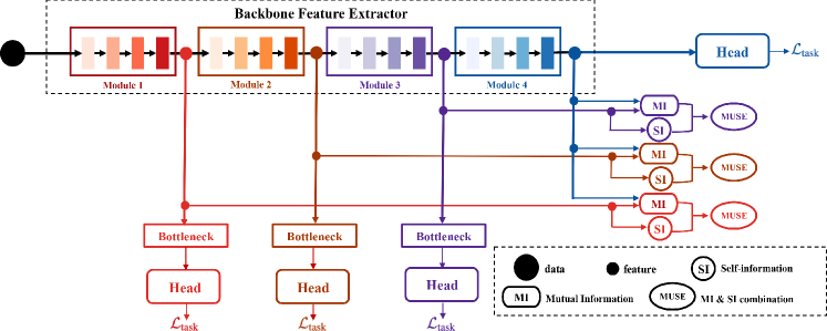
Figure 1: Illustration of self-distillation framework with MUSE. Each color denotes a different module with a task-specific head. MUSE is calculated between Module 1-3 and Module 4. The entire network is jointly trained with MUSE and a task-specific loss.

3 Methodology

We aim to leverage MI and SI to introduce strong feature dependencies and enhance feature expressivity in a CNN, thereby effectively improving the distillation frameworks on different tasks with various backbone CNN networks. At a high level, our self-distillation (SD) framework relies on multiple (three in Fig. 1) intermediate features and the last feature (e.g., features before fully-connected layers in classification networks). For each intermediate feature, we calculate two components—task-specific objective $\mathcal{L}_{\text{task}}$ and our proposed MUSE. MUSE is an effective feature discrepancy function to introduce dependencies and enhance expressivity of all features, thereby improving the overall performance and also obtaining compact yet comparably performant subnetworks.

3.1 Notation and Preliminaries

Mathematical Formulation. A CNN can be parameterized by $\{\boldsymbol{\theta}_{1},\boldsymbol{\theta}_{2},\cdots,\boldsymbol{\theta}_{T}\}$, where $T$ is the length of depth-wise decomposition and each $\boldsymbol{\theta}_{i}$ contains multiple consecutive hidden layers. Let $X\thicksim p_{\text{data}}(x)$ be a random sample drawn from the empirical data distribution, the feature at module $t$ is obtained by a nonlinear transformation $F_{t}=E_{\boldsymbol{\theta}_{<t+1}}(X)$.
Mutual Information between features. For the features $F_{i}$ and $F_{j}$ ($i<j$), the MI can be defined as conditional entropy $\mathcal{H}(F_{j}|F_{i})$ subtracted from the self-information $\mathcal{H}(F_{j})$,

$$\mathcal{I}(F_{i};F_{j})=\mathcal{H}(F_{j})-\mathcal{H}(F_{j}|F_{i})$$ (1)

Self-Information in features. SI (or entropy) quantifies the amount of information of one random variable, and can be defined as MI between identical variables. The SI of $F_{i}$ is,

$$\mathcal{H}(F_{i})=\mathcal{H}(F_{i})-\mathcal{H}(F_{i}|F_{i})=\mathcal{I}(F_{i};F_{i})$$ (2)

3.2 Proposed Method

Introducing feature dependency by Mutual Information.

Given the decomposition of $T$ modules, we have the features $\{F_{1},F_{2},\cdots,F_{T}\}$. As we aim to enhance the performance of CNNs, we choose the last feature $F_{T}$ as the base feature and introduce dependency from shallow features $\{F_{1},F_{2},...,F_{T-1}\}$ to $F_{T}$. For any module $i<T$, the pair-wise MI is

$$\mathcal{I}(F_{i};F_{T})=\mathcal{H}(F_{T})-\mathcal{H}(F_{T}|F_{i})=\mathcal{H}(F_{i})-\mathcal{H}(F_{i}|F_{T})$$ (3)

MI quantifies the dependency between two features. Therefore, we can introduce a strong dependency between each pair of features by optimizing the sum of each $\mathcal{I}(F_{i};F_{T})$. By maximizing the MI between pairs of each shallow feature and the last feature, the information shared between the feature pairs is captured and maximized. In CNNs, lower layers usually learn features of simple patterns, whereas upper layers learn more invariant and global features [Springenberg et al.(2015)Springenberg, Dosovitskiy, Brox, and Riedmiller]. The intermediate features $F_{1},...,F_{T-1}$ can gain the global information from the most parameterized and expressive feature $F_{T}$ within the CNN architecture. Meanwhile, $F_{T}$ can be aware of more local information that is likely ignored without the introduction of the dependency. To the best of our knowledge, we are the first to use mutual information to introduce the feature dependency for self-distillation in an individual network.
Prior work [Hou et al.(2019)Hou, Ma, Liu, and Loy, Zhang et al.(2019)Zhang, Song, Gao, Chen, Bao, and Ma] typically uses L2 loss to minimize the distance in the feature space. We argue that this practice is not a good proxy to introduce dependency. Minimizing L2 loss is maximizing the likelihood by assuming the data is drawn from a Gaussian distribution. For a pair of features $F_{1}\sim p(F_{1})$ and $F_{2}\sim q(F_{2})$, maximum likelihood estimation (MLE) is known to be equivalent to minimizing the KL divergence $D_{\text{KL}}(p||q)$. Therefore, the minimum is obtained when $p=q$. It necessitates two identical distributions. However, in the scenario of self-distillation, we do not expect $p=q$, as they are obtained from different layers within one single network. They depend on each other through non-linear projections, but inherently should not be identical to preserve the semantics of different features learned by the networks. In Section 4.3, we empirically demonstrate the effectiveness of MI in comparison to L2 loss.
Enhancing feature expressivity by Self-Information. In Eq. 3, MI between shallow feature $F_{i}$ and last feature $F_{T}$ can be written in two analytically equivalent ways. Since $F_{T}$ is a non-linear projection from $F_{i}$, we consider the first form $\mathcal{I}(F_{i};F_{T})=\mathcal{H}(F_{T})-\mathcal{H}(F_{T}|F_{i})$ to reflect this casual relationship between $F_{i}$ and $F_{T}$. By maximizing $\mathcal{I}(F_{i};F_{T})$, $\mathcal{H}(F_{T})$ drives $F_{T}$ to spread in the feature space, and the conditional entropy $\mathcal{H}(F_{T}|F_{i})$ enforces $F_{T}$ to be easily identified given corresponding shallow feature $F_{i}$. Besides maximizing SI of $F_{T}$, we also aim to explicitly maximize the SI of shallow features. To this end, we introduce two realizations of MUSE to combine the MI and SI as follows.
Additive Information. The intuition originates from the two forms of MI (Eq. 3). Maximizing pure MI is maximizing either form of an SI and a conditional entropy. Since both $F_{i}$ and $F_{T}$ are now dynamically learnable, they should be maximized jointly. Only the conditional entropy $\mathcal{H}(F_{T}|F_{i})$ is considered to reflect the causal order of feedforward pass. One way to maximize these terms jointly is the summation,

$$\vspace{-15pt}\mathcal{I}^{+}(F_{i},F_{T})=\mathcal{H}(F_{i})+\mathcal{H}(F_{T})-\mathcal{H}(F_{T}|F_{i})=\mathcal{H}(F_{i})+\mathcal{I}(F_{i};F_{T})$$ (4)

Eq. 4 can be interpreted as maximizing both SI of $F_{i}$ and $F_{T}$, while keeping $F_{T}$ easily identified given $F_{i}$. The proven neural MI estimator can also be used to estimate and maximize $\mathcal{H}(F_{i})$ by rewriting it as $\mathcal{I}(F_{i};F_{i})$. As we are not concerned with the precise value of MI and SI, a more stable Jensen-Shannon MI estimator [Hjelm et al.(2019)Hjelm, Fedorov, Lavoie-Marchildon, Grewal, Bachman, Trischler, and Bengio] is used, and the loss is by negating the estimation,

$$\vspace{-15pt}{\mathcal{L}}^{\text{JSD}}(F_{i};F_{T}):=\mathbb{E}_{p_{\text{data}}\times\tilde{p}_{\text{data}}}[\operatorname{sp}\big{(}T_{\phi}(f_{i}^{\prime},f_{T})\big{)}]-\mathbb{E}_{p_{\text{data}}}[-\operatorname{sp}\big{(}-T_{\phi}(f_{i},f_{T})\big{)}]$$ (5)

where $f_{i},f_{T}$ are the features given input from $p_{\text{data}}$, $f_{i}^{\prime}$ is the feature given another input from $\tilde{p}_{\text{data}}=p_{\text{data}}$. $\operatorname{sp}(\alpha)=\operatorname{log}(1+e^{\alpha})$ is the softplus function.
Multiplicative Information. The SI is a measure of information in the range of $[0,1]$. An alternative is to combine MI and SI and let the SI function as a weighting scheme,

$$\mathcal{I}^{\times}(F_{i},F_{T})=\mathcal{H}(F_{i})\times\mathcal{I}(F_{i};F_{T})$$ (6)

Our goal is to jointly maximize each MI and SI. Since both the SI and MI are non-negative, maximizing Eq. 6 can potentially result in maximizing $\mathcal{H}(F_{i})$ and $\mathcal{I}(F_{i};F_{T})$. Practically, we still use Eq. 5 as the loss of MI and SI. It is always positive, thus minimizing the multiplication of loss can have the same affect as Additive Information that minimizes each term. Importantly, Multiplicative Information introduces an interesting property where SI functions as a weighting scheme to control MI training process. The MI components of features that have higher SI loss are accordingly weighed more in the penalty function (more details in Sec. 4.3). In the following sections, we refer to our method as MUSE and use MI$+$SI or MI$\times$SI to specifically refer to the variant of Additive Information or Multiplicative Information.
Constraining features with supervision. In unsupervised representation learning, the MI estimator is shown to be sensitive to different downstream tasks [Hjelm et al.(2019)Hjelm, Fedorov, Lavoie-Marchildon, Grewal, Bachman, Trischler, and Bengio, Tschannen et al.(2020)Tschannen, Djolonga, Rubenstein, Gelly, and Lucic]. As we tend to construct dependencies between features via the lens of MI, it is essential that all features are aware of the task content. For supervised tasks, we can explicitly provide supervision to guide the learning process and improve the feature quality. To this end, each feature is accompanied by a task-specific objective. We use cross-entropy loss with logits distillation loss for the image classification task and bounding box regression loss along with focal losses on object and class for the object detection task. In Section 4.3, we show task-specific loss can improve the overall performance, though merely combining MI with SI in a task-agnostic manner can already significantly outperform other baselines. This indicates the proposed method can effectively introduce a necessary dependency between shallow features and the last feature.
Practical multi-view formulations on MI. In a CNN, deeper layers extract a high-level representation of the data while shallower layers explore local patterns better. MUSE follows [Hjelm et al.(2019)Hjelm, Fedorov, Lavoie-Marchildon, Grewal, Bachman, Trischler, and Bengio] to estimate MI by constructing the views of global and local structures (see the supplementary material for implementation details). This formulation can possibly help introduce dependencies among features from different levels, as deeper features are presumably more related to global information and shallower features contain more local information.

4 Experiments

We conduct extensive experiments on our main target, self-distillation, with various CNN architectures for image classification and object detection. We also include a variety of ablation studies to show the effectiveness of each module. Then we apply MUSE to online and offline distillation and demonstrate its effectiveness.

4.1 Image Classification

We consider a variety of backbone networks – VGG19 (BN) [Simonyan and Zisserman(2015)], ResNet [He et al.(2016)He, Zhang, Ren, and Sun], DenseNet [Huang et al.(2017)Huang, Liu, van der Maaten, and Weinberger], NASNet [Zoph et al.(2018)Zoph, Vasudevan, Shlens, and Le] and EfficientNet [Tan and Le(2019)] – on CIFAR100 [Krizhevsky(2009)], TinyImageNet, and ImageNet [Deng et al.(2009)Deng, Dong, Socher, Li, Li, and Fei-Fei]. For classification, we use labels to calculate cross-entropy at each intermediate features. We also add knowledge distillation loss [Hinton et al.(2015)Hinton, Vinyals, and Dean] as part of the task-specific loss in this line of experiments. We will further show in Section 4.3 that MUSE is necessary for the improvement without knowledge distillation loss and cross-entropy loss. For CIFAR100 and TinyImageNet, we train the networks with MUSE using SGD with momentum 0.9, weight decay 5e-4, learning rate initialized as 0.1 and divided by 10 after epoch 75, 130, and 180 for total 200 epochs. For ImageNet, we use SGD with momentum 0.9, weight decay 1e-4, and learning rate initialized as 0.1 and divided by 10 after epoch 30 and 60 for total 90 epochs. The batch size is 128, 64, and 256 for CIFAR100, TinyImageNet, and ImageNet, respectively. The depth-wise decomposition strategy empirically depends on the architecture, e.g., ResNet has 4 stages, so each stage is a module; VGG is decomposed at the positions of the first 4 maxpooling layers. More details can be found in the supplementary material.

CIFAR100	Module 1				Module 2				Module 3				Module 4
	BYOT	MI+SI	MI $\times$SI		BYOT	MI+SI	MI$\times$SI		BYOT	MI+SI	MI$\times$SI		BYOT	MI+SI	MI$\times$SI	Baseline
VGG19	$56.92_{\pm 0.15}$	$\bf{60.10_{\pm 0.11}}$	${57.21_{\pm 0.14}}$		$65.72_{\pm 0.19}$	$\bf{68.06_{\pm 0.19}}$	${66.14_{\pm 0.17}}$		$68.55_{\pm 0.17}$	$68.96_{\pm 0.18}$	$\bf{69.26_{\pm 0.18}}$		$69.79_{\pm 0.24}$	$71.07_{\pm 0.21}$	${\color[rgb]{1,0,0}\bf{71.24_{\pm 0.18}}}$	$68.57_{\pm 0.27}$
ResNet18	$67.17_{\pm 0.14}$	$67.14_{\pm 0.42}$	$\bf{68.12_{\pm 0.24}}$		$73.27_{\pm 0.19}$	$\bf{74.16_{\pm 0.13}}$	${73.98_{\pm 0.28}}$		$77.14_{\pm 0.21}$	$\bf{77.96_{\pm 0.29}}$	${77.45_{\pm 0.30}}$		$77.86_{\pm 0.30}$	$\bf{78.75_{\pm 0.31}}$	${78.37_{\pm 0.34}}$	$77.43_{\pm 0.36}$
ResNet34	$65.77_{\pm 0.07}$	$\bf{68.58_{\pm 0.37}}$	${68.47_{\pm 0.31}}$		$75.15_{\pm 0.21}$	$\bf{75.95_{\pm 0.23}}$	${74.93_{\pm 0.33}}$		$78.11_{\pm 0.17}$	$\bf{79.77_{\pm 0.20}}$	${78.91_{\pm 0.21}}$		$78.96_{\pm 0.11}$	$\bf{80.11_{\pm 0.19}}$	${79.39_{\pm 0.16}}$	$77.56_{\pm 0.24}$
ResNet50	$68.86_{\pm 0.17}$	$\bf{71.24_{\pm 0.33}}$	${69.82_{\pm 0.21}}$		$77.71_{\pm 0.16}$	$77.77_{\pm 0.27}$	$\bf{78.04_{\pm 0.13}}$		$80.04_{\pm 0.12}$	$\bf{81.25_{\pm 0.29}}$	${80.26_{\pm 0.14}}$		$80.56_{\pm 0.16}$	$\bf{81.44_{\pm 0.22}}$	${80.63_{\pm 0.16}}$	$77.80_{\pm 0.23}$
ResNet101	$71.97_{\pm 0.23}$	$72.00_{\pm 0.33}$	$\bf{72.15_{\pm 0.21}}$		$75.61_{\pm 0.21}$	$\bf{78.65_{\pm 0.34}}$	${77.06_{\pm 0.14}}$		$78.92_{\pm 0.19}$	$\bf{81.53_{\pm 0.23}}$	${80.74_{\pm 0.32}}$		$79.06_{\pm 0.27}$	$\bf{81.72_{\pm 0.37}}$	${80.89_{\pm 0.17}}$	$77.97_{\pm 0.15}$
ResNet152	$67.72_{\pm 0.21}$	$70.46_{\pm 0.33}$	$\bf{70.92_{\pm 0.23}}$		$77.82_{\pm 0.24}$	$\bf{79.53_{\pm 0.28}}$	${78.38_{\pm 0.18}}$		$79.91_{\pm 0.17}$	$\bf{81.83_{\pm 0.31}}$	${81.77_{\pm 0.21}}$		$80.73_{\pm 0.19}$	$\bf{82.09_{\pm 0.36}}$	${81.69_{\pm 0.19}}$	$78.85_{\pm 0.26}$
NASNet	${66.85_{\pm 0.21}}$	$\bf{67.45_{\pm 0.33}}$	$66.50_{\pm 0.39}$		$73.73_{\pm 0.26}$	$74.17_{\pm 0.19}$	$\bf{74.43_{\pm 0.21}}$		$75.01_{\pm 0.31}$	$\bf{76.81_{\pm 0.28}}$	${76.41_{\pm 0.33}}$		$75.85_{\pm 0.29}$	$\bf{77.11_{\pm 0.27}}$	${76.87_{\pm 0.21}}$	$75.64_{\pm 0.41}$
EfficientNet-B0	$70.21_{\pm 0.09}$	$\bf{70.96_{\pm 0.16}}$	$70.83_{\pm 0.17}$		$77.28_{\pm 0.13}$	$78.15_{\pm 0.16}$	$\bf{78.40_{\pm 0.11}}$		$77.93_{\pm 0.08}$	$78.40_{\pm 0.18}$	$\bf{78.44_{\pm 0.12}}$		$78.00_{\pm 0.14}$	$78.56_{\pm 0.14}$	$\bf{78.89_{\pm 0.12}}$	$77.61_{\pm 0.13}$

TinyImageNet	Module 1				Module 2				Module 3				Module 4
	BYOT	MI+SI	MI$\times$SI		BYOT	MI+SI	MI$\times$SI		BYOT	MI+SI	MI$\times$SI		BYOT	MI+SI	MI$\times$SI	Baseline
ResNet18	$42.06_{\pm 0.18}$	$42.34_{\pm 0.20}$	$\bf{42.54_{\pm 0.19}}$		$52.05_{\pm 0.21}$	$\bf{53.02_{\pm 0.23}}$	${52.49_{\pm 0.22}}$		$62.31_{\pm 0.25}$	$\bf{63.14_{\pm 0.19}}$	${62.98_{\pm 0.23}}$		$65.60_{\pm 0.17}$	$66.72_{\pm 0.22}$	$\bf{67.31_{\pm 0.20}}$	$64.68_{\pm 0.30}$
ResNet34	$44.02_{\pm 0.28}$	$\bf{45.71_{\pm 0.22}}$	$45.32_{\pm 0.24}$		$56.68_{\pm 0.31}$	$\bf{58.39_{\pm 0.26}}$	$58.27_{\pm 0.19}$		$66.67_{\pm 0.23}$	$67.48_{\pm 0.19}$	$\bf{67.59_{\pm 0.25}}$		$68.44_{\pm 0.25}$	$\bf{69.41_{\pm 0.31}}$	$69.13_{\pm 0.22}$	$66.72_{\pm 0.27}$
EfficientNet-B0	$53.02_{\pm 0.08}$	$53.06_{\pm 0.11}$	$\bf{55.45_{\pm 0.14}}$		$62.05_{\pm 0.11}$	$\bf{64.77_{\pm 0.16}}$	$62.51_{\pm 0.16}$		$64.91_{\pm 0.13}$	${65.30_{\pm 0.15}}$	$\bf{66.33_{\pm 0.11}}$		$65.50_{\pm 0.09}$	$65.59_{\pm 0.10}$	$\bf{66.41_{\pm 0.17}}$	$64.55_{\pm 0.14}$

ImageNet	Module 1				Module 2				Module 3				Module 4
	BYOT	MI+SI	MI$\times$SI		BYOT	MI+SI	MI$\times$SI		BYOT	MI+SI	MI$\times$SI		BYOT	MI+SI	MI$\times$SI	Baseline
ResNet18	$41.26$	$\bf{41.51}$	$41.24$		$51.94$	$\bf{52.36}$	$51.99$		$62.29$	$63.45$	$\bf{63.71}$		$69.84$	$70.35$	${\color[rgb]{1,0,0}\bf{70.57}}$	$69.64$

Table 1: Image Classification on CIFAR100 (top), TinyImageNet (middle) and ImageNet (bottom). Top-1 accuracy averaged over 3 runs, higher is better. The best of each Module is in bold. The best for an architecture is in red. MI+SI: Additive Information, MI$\times$SI: Multiplicative Information. MUSE outperforms on all modules and the baseline.

Comparison with BYOT.

MUSE is related to BYOT [Zhang et al.(2019)Zhang, Song, Gao, Chen, Bao, and Ma] in the form of module decomposition. Therefore, we decompose the backbone into 4 modules to fairly compare with BYOT [Zhang et al.(2019)Zhang, Song, Gao, Chen, Bao, and Ma]. Table 1 shows that MUSE consistently outperforms BYOT significantly for all modules on all networks. We posit that MUSE introduces the feature dependencies and enhances feature expressivity by maximizing MI and SI. Meanwhile BYOT minimizes the L2 loss in the feature space which leads to an undesirable outcome that forces the feature distributions to be identical (discussed in Section 3.2). It poses an unexpected regularization and worsens the performance. Further empirical results and discussion on MUSE as a functional proxy to introduce feature dependency can be found in Table 5 and Section 4.3. Interestingly, for the two variants of MUSE, MI$\times$SI is shown to be more likely to perform better on VGG19 and EfficientNet-B0, while MI$+$SI tends to outperform on other ResNets and NASNet. For those networks where MI$\times$SI performs worse, the performance gaps between layers are shown to be larger, and therefore different features are not comparably informative. A direct multiplication may allow the network to ignore some shallower features.

Comparison with self-distillation.

We compare MUSE to other state-of-the-art SD approaches: Class-wise Self-knowledge Distillation (CS-KD) [Yun et al.(2020)Yun, Park, Lee, and Shin], On-the-fly Native Ensemble (ONE) [Lan et al.(2018)Lan, Zhu, and Gong], Data-Distortion Guided Self-Distillation (DDGSD) [Xu and Liu(2019)], and Feature Refinement via Self-Knowledge Distillation (FRSKD) [Ji et al.(2021)Ji, Shin, Hwang, Park, and Moon]. We report the accuracy of the last module for MUSE and BYOT. Table 2 indicates that MUSE can beat all other SD methods. Note that MUSE serves as the feature discrepancy function and is therefore orthogonal to other SD methods. It can be applied to these methods and potentially further improve their performance.

Table 2: Self-distillation comparison on CIFAR100. Evaluated by top-1 accuracy over 3 runs, higher is better. Best result is in bold. $\dagger$: reported result from [Ji et al.(2021)Ji, Shin, Hwang, Park, and Moon].

Method	Baseline	CS-KD	ONE	DDGSD	BYOT	FRSKD$\dagger$	MI+SI (ours)	MI$\times$SI (ours)
ResNet18	$77.43_{\pm 0.36}$	$78.01_{\pm 0.11}$	$77.03_{\pm 0.21}$	$77.88_{\pm 0.32}$	$77.86_{\pm 0.30}$	$77.71_{\pm 0.14}$	$\bf{78.75_{\pm 0.31}}$	$78.37_{\pm 0.34}$
DenseNet121	$77.01_{\pm 0.06}$	$78.25_{\pm 0.12}$	$76.88_{\pm 0.29}$	$78.04_{\pm 0.19}$	$78.15_{\pm 0.14}$	$-$	${78.45_{\pm 0.07}}$	$\textbf{78.56}_{\pm 0.11}$

Model Compression.

Table 3: Compact networks by MUSE.

CIFAR100		Baseline				MUSE
		top-1	params	FLOPs		top-1	params	FLOPs
VGG19		$68.57$	$20.0$M	$20499$M		$69.26$	$2.3$M	$2380$M
ResNet18		$77.43$	$11.2$M	$256$M		$77.96$	$2.8$M	$248$M
ResNet34		$77.56$	$21.3$M	$393$M		$79.77$	$8.2$M	$380$M
ResNet50		$77.80$	$23.4$M	$431$M		$78.04$	$1.4$M	$370$M
ResNet101		$77.97$	$42.4$M	$507$M		$78.65$	$1.4$M	$370$M
ResNet152		$78.85$	$58.0$M	$636$M		$79.53$	$2.5$M	$441$M
NASNet		$75.64$	$5.1$M	$241$M		$76.81$	$1.9$M	$238$M
EfficientNet-B0		$77.61$	$4.0$M	$454$M		$78.40$	$0.8$M	$290$M
TinyImageNet		Baseline				MUSE
		top-1	params	FLOPs		top-1	params	FLOPs
ResNet34		$66.72$	$21.3$M	$1543$M		$67.59$	$8.2$M	$1520$M
EfficientNet-B0		$64.55$	$4.0$M	$454$M		$64.77$	$0.8$M	$290$M

In addition to improving accuracy as discussed in Section 4.1, MUSE can intrinsically achieve model compression without sacrificing performance. Since intermediate features are extracted for predictions, the models can be compressed if the prediction performance from the intermediate features outperforms the baseline. For example, Module 3 from VGG19 has higher top-1 accuracy compared to the baseline on CIFAR100 (69.26% vs. 68.57%). Hence, by training the model with MUSE, modules after Module 3 can be discarded in inference while achieving higher accuracy with less parameters and computation. Table 3 shows the comparisons between the compressed models and the corresponding baseline models shown in Table 1. All the compressed models achieve higher top-1 accuracy while the number of parameters and floating-point operations per second (FLOPs) are significantly reduced (up to $30.3\times$ and $8.6\times$, respectively). The compression ratio can be traded off for accuracy by changing the layers where intermediate features are extracted in MUSE. This approach is orthogonal to other model compression methods such as pruning and quantization and can be combined with them to further compress the models.

4.2 Object Detection

Table 4: Object Detection, mAP with 0.5 IoU. Higher is better.

Networks	YOLOv5-S	YOLOv5-M	YOLOv5-L	YOLOv5-X
Baseline	$0.549_{\pm 0.006}$	$0.619_{\pm 0.001}$	$0.641_{\pm 0.001}$	$0.663_{\pm 0.002}$
MI+SI	$0.543_{\pm 0.001}$	$0.627_{\pm 0.002}$	$0.655_{\pm 0.003}$	$0.666_{\pm 0.001}$
MI$\times$SI	$\bf{0.559_{\pm 0.001}}$	$\bf{0.629_{\pm 0.002}}$	$\bf{0.659}_{\pm 0.003}$	$\bf{0.672}_{\pm 0.001}$

We apply MUSE on the Yolov5 family for object detection on COCO [Lin et al.(2014)Lin, Maire, Belongie, Hays, Perona, Ramanan, Dollár, and Zitnick] dataset. Yolov5 models consist of a backbone and a head. The backbone is decomposed into two modules: the last 3 components (Conv, SPP, C3) and the other components in front of them. We estimate MI and SI using the features out of the two modules similar to Section 4.1. A bottleneck layer is concatenated after the first backbone module followed by a detection head (same as the original Yolov5). All networks are trained from scratch using SGD with momentum $0.937$, weight decay $0.01$, and the learning rate initialized as 0.01 and decayed to 0.002 in a sinusoidal ramp. We follow the batch size as official Yolov5 repo. As shown in Table 4, MI$\times$SI variant can improve the detection performance of all Yolov5 models. The MI$+$SI variant, on the other hand, is able to improve the mAP of Yolov5-M and Yolov5-L. Compared to image classification, low-level features like spatial locality is critical for object detection. We hypothesize that the weighting scheme in MI$\times$SI possibly attaches more importance to those shallow features, rather than equivalently optimizing all terms as in MI$+$SI.

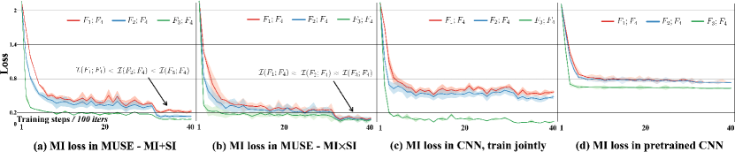
Figure 2: Training curves of MI loss on CIFAR100 EfficientNet-B0. X-axis: training steps (per 100 iterations), y-axis: loss (always positive, lower means higher MI). Red, blue, green denote MI loss between $F_{4}$ and $F_{1}$, $F_{2}$, $F_{3}$. The value of each MI loss is comparable as its implementation is same for all.

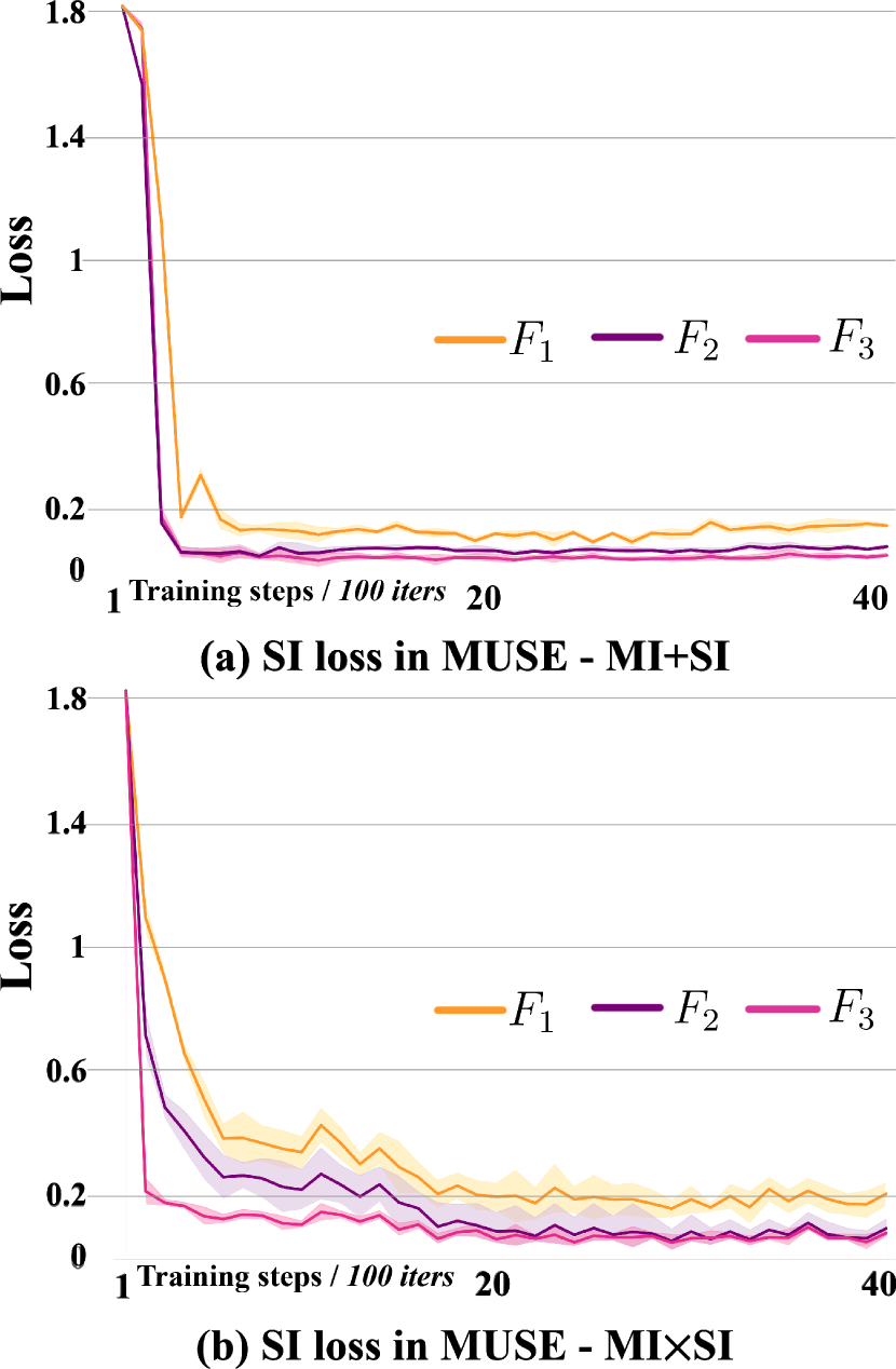
Figure 3: SI loss on CIFAR100 EfficientNet-B0 of $F_{1}$, $F_{2}$ and $F_{3}$.

4.3 Ablation study

MI & SI interaction in MUSE.

Though the MI and SI in our implementation are not precisely estimated, the decrease of the loss can indicate the relative value of MI and SI. In Fig. 2(a) and 2(b), all MI losses in MI$\times$SI converge to a similar level, whereas converged MI losses in MI$+$SI are diverse (significantly higher for shallower features). We can see in Fig. 3 that shallower features consistently have higher SI losses (lower SI) for both MI$+$SI and MI$\times$SI. Therefore for MI$\times$SI where MI loss is weighted by SI loss (always positive), the optimization of shallow features is boosted . It also explains why MI$\times$SI shows superior performance in object detection (Table 4), as the information of lower-level feature is better captured in MI$\times$SI where shallow features are weighted with more importance. Hence, shallow features tend to have lower MI losses (higher MI) in MI$\times$SI than MI$+$SI after convergence. Dense prediction like object detection may prefer such well-trained multi-scale feature information. If MI is the regularizer for CNN training, we can further interpret SI as the regularizer for the MI training.

MI in MUSE and conventional CNN.

A typical strategy (including MUSE) is to estimate and maximize MI jointly with CNN training. To compare with MI in baseline CNNs, we evaluated on MI with trainable CNN (Fig. 2 (c)) and pretrained CNN (Fig. 2 (d)) for a full picture of MI in baseline CNNs (EfficientNet in this example). Note that the implementation of Fig. 2 (c) is the same as only MI in Table 5. The last MI loss between $F_{3};F_{4}$ can still converge to a very low value but the other two are poorly optimized, indicating the effectiveness of SI in MUSE to control the MI training process. In Fig. 2 (d), the MI losses in the pretrained CNN cannot converge to a stage as low as the other three. We speculate it is because—(1) the MI between intermediate features of conventional CNNs are possibly much lower; (2) The MI estimators cannot work properly without trainable parameters of the backbone.

Table 5: Different terms in MUSE.

Backbone	ResNet18	EfficientNet-B0
Baseline	$77.43_{\pm 0.36}$	$77.61_{\pm 0.13}$
CE	$77.66_{\pm 0.27}$	$77.94_{\pm 0.11}$
CE + KD	$77.98_{\pm 0.21}$	$78.06_{\pm 0.18}$
L2	$77.18_{\pm 0.23}$	$77.43_{\pm 0.18}$
L2 + CE	$77.65_{\pm 0.25}$	$77.51_{\pm 0.16}$
L2 + CE + KD	$77.86_{\pm 0.30}$	$78.00_{\pm 0.14}$
MI	$77.95_{\pm 0.31}$	$77.67_{\pm 0.26}$
SI	$77.81_{\pm 0.44}$	$77.69_{\pm 0.25}$
MI + CE	$78.07_{\pm 0.33}$	$78.07_{\pm 0.11}$
MI + CE + KD	$78.22_{\pm 0.21}$	$78.35_{\pm 0.13}$
(MI+SI)	$78.14_{\pm 0.25}$	$77.83_{\pm 0.19}$
(MI$\times$SI)	$78.06_{\pm 0.29}$	$77.91_{\pm 0.24}$
(MI+SI) + CE	$78.63_{\pm 0.26}$	$78.46_{\pm 0.17}$
(MI$\times$SI) + CE	$78.35_{\pm 0.24}$	$78.81_{\pm 0.12}$
(MI+SI) + CE + KD	$\bf{78.75_{\pm 0.31}}$	$78.56_{\pm 0.14}$
(MI$\times$SI) + CE + KD	$78.37_{\pm 0.34}$	$\bf{78.89_{\pm 0.12}}$

Effectiveness of different modules.

In Section 4.1, we empirically show MUSE outperforms other SOTA SD methods. As our objective incorporates multiple terms including classification loss (cross-entropy) and knowledge distillation loss (KL divergence between logits), we conduct experiments with individual terms as in Table 5. We report the top-1 accuracy at Module 4 with 3 runs. CE and KD denote cross-entropy and knowledge distillation loss between intermediate features. We decompose the networks into 4 modules and all terms (CE, KD, L2, MI, and MUSE) are calculated between Module 1-3 and Module 4. In Table 5, we can observe: (1) CE and KD can improve the overall performance without other feature discrepancy functions; (2) L2 loss itself hurts the original performance, while MI, MI+SI, and MI$\times$SI can further improve the performance with CE and KD. It corroborates with the argument in Section 3.2 that MI serves as a more functional proxy to introduce dependencies between intermediate features; (3) MUSE, including both MI+SI and MI$\times$SI, outperforms MI, indicating the effectiveness of combining MI and SI; (4) MUSE can improve the network even without CE and KD, showing that MI and SI can learn more useful features without explicit supervision to the intermediate features; (5) Though MUSE solely improves the performance, adding CE & KD together provides the maximum improvement. MI estimators are sensitive to the tasks, therefore explicit supervision likely helps introduce meaningful feature dependencies for specific tasks; (6) Using MI or SI solely provides marginal improvement, while combining them performs the best.

Advantages over other discrepancy functions.

Table 6: Feature discrepancy.

Backbone	ResNet18	EfficientNet-B0
Baseline	$77.43_{\pm 0.36}$	$77.61_{\pm 0.13}$
L2	$77.65_{\pm 0.25}$	$77.51_{\pm 0.16}$
MMD	$76.22_{\pm 0.19}$	$77.03_{\pm 0.16}$
adversarial	$78.18_{\pm 0.18}$	$78.25_{\pm 0.14}$
VID	$76.97_{\pm 0.54}$	$77.37_{\pm 0.35}$
MI+SI	$\bf{78.63_{\pm 0.26}}$	$78.46_{\pm 0.17}$
MI$\times$SI	$78.35_{\pm 0.24}$	$\bf{78.81_{\pm 0.12}}$

Prior distillation works introduce feature dependencies via different feature discrepancy functions, such as L2 loss [Romero et al.(2015)Romero, Ballas, Kahou, Chassang, Gatta, and Bengio, Zagoruyko and Komodakis(2017)], Maximum Mean Discrepancy (MMD) [Huang and Wang(2017)], adversarial loss [Chung et al.(2020)Chung, Park, Kim, and Kwak] and VID (a type of MI estimated by variational bound [Ahn et al.(2019)Ahn, Hu, Damianou, Lawrence, and Dai]). To demonstrate the effectiveness of MUSE on SD, we apply these feature discrepancy functions to introduce the feature dependencies and compare to our proposed MUSE in Table 6. All networks incorporate CE loss to provide explicit supervision. KD loss is not included in Table 6 to better show the improvement from the feature discrepancy functions. We observe a consistent improvement of MUSE over other functions: (1) L2 loss, often used in offline distillation, cannot consistently improve performance. It demonstrates our argument that enforcing the features to be identical (as L2 loss does) cannot introduce useful dependencies in SD; (2) MMD is the same as L2 that its minimum is obtained if and only if the two features are identical; (3) Adversarial loss differently shows significant improvement over baselines. Minimizing L2 loss is equivalent to minimizing the KL divergence between two features $D_{\text{KL}}(p_{1}||p_{2})$ ($p$ is the probability density), while minimizing adversarial loss is equivalent to minimizing the Jensen–Shannon (JS) divergence [Goodfellow et al.(2014)Goodfellow, Pouget-Abadie, Mirza, Xu, Warde-Farley, Ozair, Courville, and Bengio] between two features. It is a symmetric version of KL divergence that $D_{\text{JS}}(p_{1}||p_{2})=D_{\text{JS}}(p_{2}||p_{1})$. As both features are not known, a symmetric discrepancy function without assumption on the direction is possibly preferred. This also explains its empirical success in online distillation [Chung et al.(2020)Chung, Park, Kim, and Kwak]. Yet, its minimum is obtained if and only if two features are identical, which weakens its faculty in SD; (4) MUSE outperforms MI estimated by variational bound [Ahn et al.(2019)Ahn, Hu, Damianou, Lawrence, and Dai], as this bound of MI only holds in the offline distillation where the pretrained teacher is static (refer to Eq.3 and 4 in VID [Ahn et al.(2019)Ahn, Hu, Damianou, Lawrence, and Dai]).
Extension to Offline / Online Distillation. We have shown that MUSE necessarily improves the SD framework on image classification and object detection. We further investigate its potential application on offline and online distillation where the features are from different CNNs. MUSE can be readily applied in this scenario by replacing the own last feature of a CNN with the last feature of another teacher network. We also follow our previous experimental setting to decompose the student network into four modules. To establish a fair comparison, we do not include CE and KD loss for intermediate features, but only calculate MUSE between intermediate features of the student network and the last feature of the teacher network. We follow a traditional strategy to add KD loss on the last layer of the student network. For online distillation, we consider two settings: two identical networks and two different networks. We report the average accuracy for two identical networks. For offline distillation, we use the fixed last feature of the teacher network to calculate MUSE. In Table 7, we can observe consistent improvement from MUSE for online distillation, and comparable performance with the state-of-the-art for offline distillation.

Net1 / resnet20 / resnet56 / resnet20 / ShuffleNetV1 [Zhang et al.(2018)Zhang, Zhou, Lin, and Sun] / Net2 resnet20 resnet56 resnet56 WRN-40-2 [Zagoruyko and Komodakis(2016)] Baseline $69.06$ $72.34$ $69.06/72.34$ $70.50/75.61$ KD $70.51$ $75.24$ $70.11/74.69$ $70.50/75.61$ DML [Zhang et al.(2017)Zhang, Xiang, Hospedales, and Lu] $70.84$ $75.63$ $71.13/74.97$ $75.89/78.16$ KDCL [Guo et al.(2020)Guo, Wang, Wu, Yu, Liang, Hu, and Luo] $70.23$ $75.28$ $70.36/74.83$ $74.79/77.53$ AFD [Chung et al.(2020)Chung, Park, Kim, and Kwak] $70.63$ $75.40$ $71.22/75.12$ $75.39/77.13$ MI+SI $\bf{71.02_{\pm 0.14}}$ $\bf{76.02_{\pm 0.13}}$ $\bf{71.34_{\pm 0.16}}/\bf{75.55_{\pm 0.08}}$ $76.65_{\pm 0.19}/\bf{78.51_{\pm 0.17}}$ MI$\times$SI $70.71_{\pm 0.16}$ $75.80_{\pm 0.15}$ $71.05_{\pm 0.11}/75.17_{\pm 0.10}$ $\bf{76.80_{\pm 0.21}}$$/78.34_{\pm 0.15}$

Teacher resnet56 (72.34) resnet110 (74.31) Student resnet20 resnet32 Baseline $69.06$ $71.14$ KD [Hinton et al.(2015)Hinton, Vinyals, and Dean] $70.66$ $73.08$ FitNets [Romero et al.(2015)Romero, Ballas, Kahou, Chassang, Gatta, and Bengio] $69.21$ $71.06$ VID [Ahn et al.(2019)Ahn, Hu, Damianou, Lawrence, and Dai] $70.38$ $72.61$ CRD [Tian et al.(2020a)Tian, Krishnan, and Isola] $71.16$ $\bf{73.48}$ MI+SI $\bf{71.30_{\pm 0.09}}$ $73.34_{\pm 0.17}$ MI$\times$SI $71.27_{\pm 0.22}$ $\bf{73.48_{\pm 0.29}}$

(a) Online Distillation.

(b) Offline Distillation.

Table 7: Traditional distillation with MUSE. Evaluated by top-1 accuracy. (a) Two settings are considered in online distillation—two identical networks (averaged accuracy is reported) and two different networks; (b) Pretrained teacher networks in offline distillation are static.

5 Conclusion

We propose a novel feature discrepancy function—MUSE, based on effective neural estimators of MI and SI. We present two variants of MUSE to combine MI and SI. We argue and empirically demonstrate on extensive experiments that MUSE is a more effective feature discrepancy function for knowledge distillation. Especially on self-distillation, MUSE necessarily introduces dependencies among features in a CNN, thereby significantly improving the performance and obtaining more compact yet comparably performant subnetworks. MUSE shows superior performance on image classification and object detection. By drawing the features from different levels, MUSE can possibly be extended to architectures like RNN or attention models. The level may not necessarily be the depth of the network, rather time steps or sequential order. We leave these as future work on improving MUSE.

References

- [Ahn et al.(2019)Ahn, Hu, Damianou, Lawrence, and Dai] Sungsoo Ahn, Shell Xu Hu, Andreas Damianou, Neil D. Lawrence, and Zhenwen Dai. Variational information distillation for knowledge transfer. In Proceedings of the IEEE Conference on Computer Vision and Pattern Recognition (CVPR), 2019.
- [Bachman et al.(2019)Bachman, Hjelm, and Buchwalter] Philip Bachman, R Devon Hjelm, and William Buchwalter. Learning representations by maximizing mutual information across views. In Advances in Neural Information Processing Systems (NeurIPS), 2019.
- [Belghazi et al.(2018)Belghazi, Baratin, Rajeshwar, Ozair, Bengio, Courville, and Hjelm] Mohamed Ishmael Belghazi, Aristide Baratin, Sai Rajeshwar, Sherjil Ozair, Yoshua Bengio, Aaron Courville, and Devon Hjelm. Mutual information neural estimation. In Proceedings of International Conference on Machine Learning (ICML), 2018.
- [Chung et al.(2020)Chung, Park, Kim, and Kwak] Inseop Chung, SeongUk Park, Jangho Kim, and Nojun Kwak. Feature-map-level online adversarial knowledge distillation. In Proceedings of International Conference on Machine Learning (ICML), 2020.
- [Deng et al.(2009)Deng, Dong, Socher, Li, Li, and Fei-Fei] Jia Deng, Wei Dong, Richard Socher, Li-Jia Li, Kai Li, and Li Fei-Fei. Imagenet: A large-scale hierarchical image database. In Proceedings of the IEEE Conference on Computer Vision and Pattern Recognition (CVPR), 2009.
- [Goodfellow et al.(2014)Goodfellow, Pouget-Abadie, Mirza, Xu, Warde-Farley, Ozair, Courville, and Bengio] Ian J. Goodfellow, Jean Pouget-Abadie, Mehdi Mirza, Bing Xu, David Warde-Farley, Sherjil Ozair, Aaron Courville, and Yoshua Bengio. Generative adversarial nets. In Advances in Neural Information Processing Systems (NIPS), 2014.
- [Guo et al.(2020)Guo, Wang, Wu, Yu, Liang, Hu, and Luo] Qiushan Guo, Xinjiang Wang, Yichao Wu, Zhipeng Yu, Ding Liang, Xiaolin Hu, and Ping Luo. Online knowledge distillation via collaborative learning. In Proceedings of the IEEE Conference on Computer Vision and Pattern Recognition (CVPR), 2020.
- [He et al.(2016)He, Zhang, Ren, and Sun] Kaiming He, Xiangyu Zhang, Shaoqing Ren, and Jian Sun. Deep residual learning for image recognition. In Proceedings of the IEEE Conference on Computer Vision and Pattern Recognition (CVPR), 2016.
- [Hinton et al.(2015)Hinton, Vinyals, and Dean] Geoffrey Hinton, Oriol Vinyals, and Jeff Dean. Distilling the knowledge in a neural network. arXiv preprint arXiv:1503.02531, 2015.
- [Hjelm et al.(2019)Hjelm, Fedorov, Lavoie-Marchildon, Grewal, Bachman, Trischler, and Bengio] R Devon Hjelm, Alex Fedorov, Samuel Lavoie-Marchildon, Karan Grewal, Phil Bachman, Adam Trischler, and Yoshua Bengio. Learning deep representations by mutual information estimation and maximization. In Proceedings of International Conference on Learning Representations (ICLR), 2019.
- [Hou et al.(2019)Hou, Ma, Liu, and Loy] Yuenan Hou, Zheng Ma, Chunxiao Liu, and Chen Change Loy. Learning lightweight lane detection cnns by self attention distillation. In Proceedings of the IEEE International Conference on Computer Vision (ICCV), 2019.
- [Huang et al.(2017)Huang, Liu, van der Maaten, and Weinberger] Gao Huang, Zhuang Liu, Laurens van der Maaten, and Kilian Q Weinberger. Densely connected convolutional networks. In Proceedings of the IEEE Conference on Computer Vision and Pattern Recognition (CVPR), 2017.
- [Huang and Wang(2017)] Zehao Huang and Naiyan Wang. Like what you like: Knowledge distill via neuron selectivity transfer. arXiv preprint arXiv:1707.01219, 2017.
- [Hulle(2005)] Marc M. Van Hulle. Edgeworth approximation of multivariate differential entropy. Neural computation,, 2005.
- [Ji et al.(2021)Ji, Shin, Hwang, Park, and Moon] Mingi Ji, Seungjae Shin, Seunghyun Hwang, Gibeom Park, and Il-Chul Moon. Refine myself by teaching myself: Feature refinement via self-knowledge distillation. In Proceedings of the IEEE Conference on Computer Vision and Pattern Recognition (CVPR), 2021.
- [Kinney and Atwal(2014)] Justin B. Kinney and Gurinder S. Atwal. Equitability, mutual information, and the maximal information coefficient. Proceedings of the National Academy of Sciences, 2014.
- [Kraskov et al.(2004)Kraskov, Stögbauer, and Grassberger] Alexander Kraskov, Harald Stögbauer, and Peter Grassberger. Estimating mutual information. Physical Review E, 2004.
- [Krizhevsky(2009)] Alex Krizhevsky. Learning multiple layers of features from tiny images. Technical report, University of Toronto, 2009.
- [Lan et al.(2018)Lan, Zhu, and Gong] Xu Lan, Xiatian Zhu, and Shaogang Gong. Knowledge distillation by on-the-fly native ensemble. In Advances in Neural Information Processing Systems (NeurIPS), 2018.
- [Lin et al.(2014)Lin, Maire, Belongie, Hays, Perona, Ramanan, Dollár, and Zitnick] Tsung-Yi Lin, Michael Maire, Serge Belongie, James Hays, Pietro Perona, Deva Ramanan, Piotr Dollár, and C Lawrence Zitnick. Microsoft coco: Common objects in context. In Proceedings of the European Conference on Computer Vision (ECCV), 2014.
- [Nemenman et al.(2004)Nemenman, Bialek, and de Ruyter van Steveninck] Ilya Nemenman, William Bialek, and Rob de Ruyter van Steveninck. Entropy and information in neural spike trains: Progress on the sampling problem. Physical Review E, 2004.
- [Oord et al.(2018)Oord, Li, and Vinyals] Aaron van den Oord, Yazhe Li, and Oriol Vinyals. Representation learning with contrastive predictive coding. arXiv preprint arXiv:1807.03748, 2018.
- [Romero et al.(2015)Romero, Ballas, Kahou, Chassang, Gatta, and Bengio] Adriana Romero, Nicolas Ballas, Samira Ebrahimi Kahou, Antoine Chassang, Carlo Gatta, and Yoshua Bengio. Fitnets: Hints for thin deep nets. In Proceedings of the International Conference on Learning Representations (ICLR), 2015.
- [Shen et al.(2019)Shen, He, and Xue] Zhiqiang Shen, Zhankui He, and Xiangyang Xue. Meal: Multi-model ensemble via adversarial learning. In Proceedings of the AAAI Conference on Artificial Intelligence (AAAI), 2019.
- [Simonyan and Zisserman(2015)] Karen Simonyan and Andrew Zisserman. Very deep convolutional networks for large-scale image recognition. In Proceedings of the International Conference on Learning Representations (ICLR), 2015.
- [Springenberg et al.(2015)Springenberg, Dosovitskiy, Brox, and Riedmiller] J.T. Springenberg, A. Dosovitskiy, T. Brox, and M. Riedmiller. Striving for simplicity: The all convolutional net. In Proceedings of the International Conference on Learning Representations (ICLR), 2015.
- [Tan and Le(2019)] Mingxing Tan and Quoc Le. EfficientNet: Rethinking model scaling for convolutional neural networks. In Proceedings of the International Conference on International Conference on Machine Learning (ICML), 2019.
- [Tian et al.(2020a)Tian, Krishnan, and Isola] Yonglong Tian, Dilip Krishnan, and Phillip Isola. Contrastive representation distillation. In Proceedings of the International Conference on Learning Representations (ICLR), 2020a.
- [Tian et al.(2020b)Tian, Krishnan, and Isola] Yonglong Tian, Dilip Krishnan, and Phillip Isola. Contrastive multiview coding. In Proceedings of the European Conference on Computer Vision (ECCV), 2020b.
- [Tschannen et al.(2020)Tschannen, Djolonga, Rubenstein, Gelly, and Lucic] Michael Tschannen, Josip Djolonga, Paul K. Rubenstein, Sylvain Gelly, and Mario Lucic. On mutual information maximization for representation learning. In Proceedings of the International Conference on Learning Representations (ICLR), 2020.
- [Xu and Liu(2019)] Ting-Bing Xu and Cheng-Lin Liu. Data-distortion guided self-distillation for deep neural networks. In Proceedings of the AAAI Conference on Artificial Intelligence (AAAI), 2019.
- [Yang et al.(2019)Yang, Xie, Su, and Yuille] Chenglin Yang, Lingxi Xie, Chi Su, and Alan L Yuille. Snapshot distillation: Teacher-student optimization in one generation. In Proceedings of the IEEE Conference on Computer Vision and Pattern Recognition (CVPR), 2019.
- [Yun et al.(2020)Yun, Park, Lee, and Shin] Sukmin Yun, Jongjin Park, Kimin Lee, and Jinwoo Shin. Regularizing class-wise predictions via self-knowledge distillation. In Proceedings of the IEEE Conference on Computer Vision and Pattern Recognition (CVPR), 2020.
- [Zagoruyko and Komodakis(2016)] Sergey Zagoruyko and Nikos Komodakis. Wide residual networks. In British Machine Vision Conference (BMVC), 2016.
- [Zagoruyko and Komodakis(2017)] Sergey Zagoruyko and Nikos Komodakis. Paying more attention to attention: Improving the performance of convolutional neural networks via attention transfer. In Proceedings of the International Conference on Learning Representations (ICLR), 2017.
- [Zhang et al.(2019)Zhang, Song, Gao, Chen, Bao, and Ma] Linfeng Zhang, Jiebo Song, Anni Gao, Jingwei Chen, Chenglong Bao, and Kaisheng Ma. Be your own teacher: Improve the performance of convolutional neural networks via self distillation. In Proceedings of the IEEE International Conference on Computer Vision (ICCV), 2019.
- [Zhang et al.(2018)Zhang, Zhou, Lin, and Sun] Xiangyu Zhang, Xinyu Zhou, Mengxiao Lin, and Jian Sun. Shufflenet: An extremely efficient convolutional neural network for mobile devices. In Proceedings of the IEEE Conference on Computer Vision and Pattern Recognition (CVPR), 2018.
- [Zhang et al.(2017)Zhang, Xiang, Hospedales, and Lu] Ying Zhang, Tao Xiang, Timothy M. Hospedales, and Huchuan Lu. Deep mutual learning. In Proceedings of the IEEE Conference on Computer Vision and Pattern Recognition (CVPR), 2017.
- [Zoph et al.(2018)Zoph, Vasudevan, Shlens, and Le] Barret Zoph, Vijay Vasudevan, Jonathon Shlens, and Quoc V. Le. Learning transferable architectures for scalable image recognition. In Proceedings of the IEEE Conference on Computer Vision and Pattern Recognition (CVPR), 2018.