QuantifyML: How Good is my Machine Learning Model?

Abstract

The efficacy of machine learning models is typically determined by computing their accuracy on test data sets. However, this may often be misleading, since the test data may not be representative of the problem that is being studied. With QuantifyML we aim to precisely quantify the extent to which machine learning models have learned and generalized from the given data. Given a trained model, QuantifyML translates it into a C program and feeds it to the CBMC model checker to produce a formula in Conjunctive Normal Form (CNF). The formula is analyzed with off-the-shelf model counters to obtain precise counts with respect to different model behavior. QuantifyML enables i) evaluating learnability by comparing the counts for the outputs to ground truth, expressed as logical predicates, ii) comparing the performance of models built with different machine learning algorithms (decision-trees vs. neural networks), and iii) quantifying the safety and robustness of models.

1 Introduction

Recent years have seen a surge in the use of machine learning algorithms in a variety of applications to analyze and learn from large amounts of data. For instance, decision-trees are a popular class of supervised learning that can learn easily-interpretable rules from data. They have found success in areas such as medical diagnosis and credit scoring [22, 5]. Deep Neural Networks (DNN) also have gained popularity in diverse fields such as banking, health-care, image and speech recognition, as well as perception in self-driving cars [15, 20].

Such machine learning models are typically evaluated by computing their accuracy on held-out test data sets, to determine how well the model learned and generalized from the training data. However, this is an imperfect measure, as they may not cover well the desired input space. Furthermore, it is often not clear which learning algorithm or trained model is better suited for a particular problem (e.g., neural networks vs. decision trees), and simply comparing the accuracy of different models may lead to misleading results. It may also be the case that well-trained models may be vulnerable to adversarial attacks [28, 25, 16] or they may violate desired safety properties [24]. It is unclear how to quantify the extent to which these vulnerabilities affect the performance of a model, as evaluating the model on the available test or adversarial data sets may again give imprecise results.

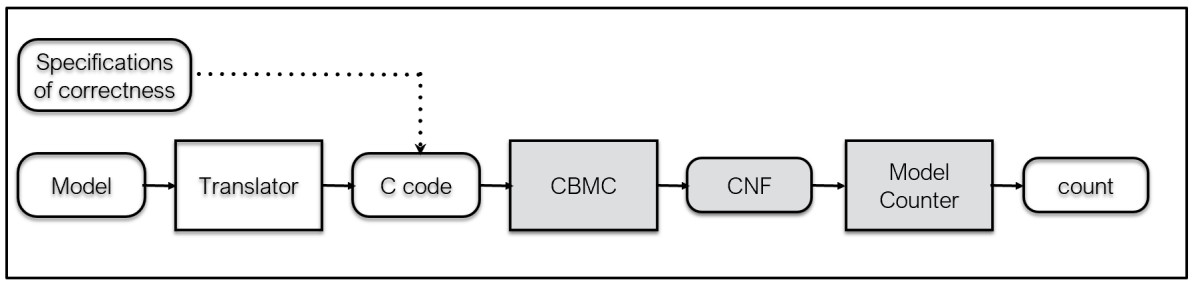
Figure 1: QuantifyML Framework

We present QuantifyML, an analysis tool that aims to precisely quantify the learnability, safety and robustness of machine learning models. In this tool, a given trained model is translated into a C program, enabling the application of the CBMC tool [21] to obtain a formula in Conjunctive Normal Form (CNF), which in turn can be analyzed with approximate and exact model counters [12, 7, 11] to obtain precise counts of the inputs that lead to different outputs. Figure 1 gives a high-level description of QuantifyML. We demonstrate QuantifyML in the context of decision trees and neural networks for the problems of learning relational properties of graphs, image classification and aircraft collision avoidance.

We derive inspiration from a recent paper [30] which presents Model Counting meets Machine Learning (MCML) to evaluate the learnability of binary decision trees. With QuantifyML we generalize MCML by providing a more general tool that can handle more realistic multi-class problems, such as decision trees with non-binary inputs and with more than two output decisions, and also neural networks. Other learning algorithms can be accommodated provided that the learned models are translated into C programs. QuantifyML’s applications extend beyond MCML and include: (i) comparison of the performance of different models, built with different learning algorithms, (ii) quantification of robustness in image classifiers, and (iii) quantification of safety of neural network models.

2 Background

Decision Trees: Decision tree learning [27] is a supervised learning technique for extracting rules that act as classifiers. Given a set of data labeled to respective classes, decision tree learning aims to discover rules in terms of the attributes of the data to discriminate one label from the other. It builds a tree such that each path of the tree encodes a rule as a conjunction of predicates on the data attributes. Each rule attempts to cluster or group inputs that belong to a certain label.

Neural Networks: Neural networks [13] are machine learning algorithms that can be trained to perform different tasks such as classification and regression. Neural networks consist of multiple layers, starting from the input layer, followed by one or more hidden layers (such as convolutional, dense, activation, and pooling), and a final decision layer. Each layer consists of a number of computational units, called neurons. Each neuron applies an activation function on a weighted sum of its inputs; $N(X)=\sigma(\sum_{\_}iw_{\_}i\cdot N_{\_}i(X)+b)$ where $N_{\_}i$ denotes the value of the $i^{th}$ neuron in the previous layer of the network and the coefficients $w_{\_}i$ and the constant $b$ are referred to as weights and bias, respectively; $\sigma$ represents the activation function. The final decision layer (also known as logits) typically uses a specialized function (e.g., max or softmax) to determine the decision or the output of the network.

Bounded Model Checking for C programs: Bounded model checking [6] is a popular technique for verifying safety properties of software systems. Given a bound on the input domain and a bound on the length of executions, a boolean formula is generated that is satisfiable if there exists an error trace or counter-example to the given property. The formula is checked using off-the-shelf decision procedures. CBMC [9] is a tool that performs analysis of programs written in a high-level language such as C, C++ or Java by applying bounded model checking. The program is first converted into a control flow graph (CFG) representation and formulas are built for the paths in the CFG leading to assertions. The model checking problem is reduced to determining the validity of a set of bit-vector equations, which are then flatted out to conjunctive normal form (CNF) and checked for satisfiability. In this work, we leverage CBMC to build the CNF formulas corresponding to the paths in the C program representation of a machine learning model. We then pass on the formulas corresponding to the respective output classes to a model counting tool in order to quantify the number of solutions.

Projected model counting: Many tools, including CBMC, translate a boolean formula to CNF by introducing auxiliary variables. These variables do not affect the satisfiability of the boolean formula but do affect the model counts. In such scenarios, projected model counting [4] needs to be used. Consider the set $M$ consisting of all variables in a boolean formula and $N$ be a subset of variables in the formula. The solutions in which the value of at least one variable in $N$ is different is considered a unique solution in the projected model counting problem. The variables in $N$ are known as primary variables and the rest of the variables are known as auxiliary variables. Please refer to [29] for a detailed discussion on model counting, projected model counting and model counters. In our work we use projected model counting, where the inputs to the model are considered as primary variables. We used two state-of-the-art model counters i.e., projMC [23] and ApproxMC [8].

MCML: MCML [30] uses model counting to perform a quantitative assessment of the performance of decision-tree classifier models. The ground truth ($\phi$) is translated by the Alloy analyzer with respect to bound $b$ into a CNF formula $cnf_{\_}{\phi}$. It then translates the relevant parts of decision tree with respect to the desired metrics (True Positives, False Positives, False Negatives, True Negatives) into a CNF formula $cnf_{\_}{d}$. It then combines these two formulas to create the CNF formula $cnf_{\_}{\phi,d}$ which is an input to the model counter that outputs the number of solutions that satisfy the formula. This count quantifies the true performance of the decision tree. MCML is limited to binary decision trees and has been used on decision-tree models when used to learn relational properties of graphs. QuantifyML goes beyond MCML as it enables quantification of the performance of more general machine learning models, that may have non-binary inputs and multi-class outputs. Our evaluation presents applications such as robustness analysis of decision-tree models on an image-classification problem (MNIST), comparison of neural network and decision-tree models for learning relational properties of graphs, and evaluation of safety for collision avoidance, which cannot be achieved with the MCML tool.

3 Approach

Quantifying the learnability of machine learning models: QuantifyML can be used to quantify the learnability of models, provided that a predicate is given which describes the ground-truth output for any input and finite bounds on the input space. Consider a model classifying a given input into one of $L$ labels. For each output label $l$, two predicate functions are generated; $\phi_{\_}{l}(x)$ which returns 1 if the output of the model is $l$ for a given input $x$ and returns 0 otherwise, and $\psi_{\_}{l}(x)$ which returns 1 if the ground-truth for the given input $x$ is $l$ and returns 0 otherwise. These predicates are used to encode the following metrics for each label $l$; True Positives (TP): $\;MC(\>CNF(\>\psi_{\_}{l}(x)\,\wedge\,\phi_{\_}{l}(x)\>),N)$, False Positives (FP): $\;MC(\>CNF(\>\neg\psi_{\_}{l}(x)\,\wedge\,\phi_{\_}{l}(x)\>),N)$, True Negatives (TN): $\;MC(\>CNF(\>\neg\psi_{\_}{l}(x)\,\wedge\,\neg\phi_{\_}{l}(x)\>),N)$, and False Negatives (FN): $\;MC(\>CNF(\>\psi_{\_}{l}(x)\,\wedge\,\neg\phi_{\_}{l}(x)\>),N)$. $N$ is the scope or bound on the input domain, $CNF$ represents a function that translates C program to formulas in the CNF form, and $MC$ represents a function that uses the projected model counter to return the number of solutions projected to the input variables. QuantifyML then uses these counts to assess the quality of the model using standard measures such as Accuracy, Precision, Recall and F1-score for the model. Accuracy=$\frac{TP+TN}{TP+FP+TN+FN}$, Precision=$\frac{TP}{TP+FP}$, Recall= $\frac{TP}{TP+FN}$ and F1-score= $\frac{2*Precision*Recall}{Precision+Recall}$.

Quantifying the safety of machine learning models: QuantifyML can also be used to quantify the extent to which input-output safety properties are satisfied for a model. Assume a property $p$ of the form ($Pre=>Post$) where $Pre$ is a condition on the input variables and $Post$ is a condition on the output of the model, such as a classifier producing a certain label. We can use QuantifyML to obtain the following counts: i) QuantifyML${}_{\_}S$ denoting the portion of the inputs for which the model satisfies the given property, and ii) QuantifyML${}_{\_}N$ denoting the portion of the inputs for which the model violates the property. These counts are then used to obtain an accuracy metric; QuantifyML${}_{\_}{Acc}$=$\frac{\emph{QuantifyML${}_{\_}S$}}{\emph{QuantifyML${}_{\_}N$}+\emph{QuantifyML${}_{\_}S$}}$, which is a measure of the extent to which the network satisfies the property.

Quantifying Local Robustness: The challenge with the analysis of more realistic models is that we typically do not have the ground truth. Image classification is such a problem, where it is not feasible to define a specification that can automatically generate the ground-truth label for any arbitrary image. However, images that are similar to, or are in close proximity (in terms of distance in the input space) to an image with a known label can be expected to have the same label. This property is called robustness in the literature. Current techniques [14, 3, 10] typically search for the existence of an adversarial input ($x^{\prime}$) within an $\epsilon$ ball surrounding a labelled input ($x$); e.g., $||x-x^{\prime}||_{\_}{\infty}\leq\epsilon$ (here the distance is in terms of the $L_{\_}{\infty}$ metric) such that the output of the model on $x$ and $x^{\prime}$ is different. When no such input exists, the model is declared robust, however, in the presence of an adversarial input there is no further information available. QuantifyML can be used to quantify robustness of machine learning models, where instead of using a predicate encoding the ground truth, we encode the local robustness requirement that the model should give the same output within the region defined by $||x-x^{\prime}||_{\_}{\infty}\leq\epsilon$. In order to quantify local robustness around a concrete n-dimensional input $x=(x_{\_}0,x_{\_}1,..x_{\_}n)$, we first define an input region $R_{\_}\epsilon$ by constraining the inputs across each dimension to be within $[x_{\_}i-\epsilon,x_{\_}i+\epsilon]$ in the translated C program. We then define Robustness${}_{\_}{\epsilon}$ as $\frac{MC(CNF(\phi_{\_}{l}(x)),R_{\_}\epsilon)}{|R_{\_}\epsilon|}$, where $\phi_{\_}{l}(x)$ is defined as before as a predicate which returns 1 if the output of the model is $l$ and 0 otherwise, $R_{\_}\epsilon$ defines the scope for the check, and $|R_{\_}\epsilon|$ quantifies its size. Intuitively, Robustness${}_{\_}{\epsilon}$ quantifies the portion of the input on which the model is robust, within the small region described by $R_{\_}\epsilon$.

Please check longer version of this paper [2] for more details on the approach. The tool currently supports decision trees trained using Scikit-Learn [26] and neural networks trained in Keras [19].

4 Evaluation

We present experiments we have performed to evaluate the benefits of using QuantifyML in the applications of quantifying learnability, safety and robustness of machine learning models.

Quantifying the learnability of machine learning models: This study aims to assess QuantifyML in quantifying the true performance of models and enabling one to compare different models, and different learning algorithms, for a given problem.

We evaluated the performance of trained models against ground truth predicates on the problem of learning relational properties of graphs. We considered 11 relational properties of graphs including Antisymmetric, Connex, Equivalence, Irreflexive, NonStrictOrder, PartialOrder, PreOrder, Reflexive, StrictOrder, TotalOrder and Transitive (refer [2]). We used the Alloy tool [17] to create datasets containing positive and negatives solutions for each of these properties. Each input in the dataset corresponds to a graph with a finite number of nodes and is represented as an adjacency matrix. Each input has a corresponding binary label (1 if the graph satisfies the respective property, 0 otherwise). Please refer [2] for more details on the setup. The problem of learning relational properties of graphs albeit seems fairly simple with binary decisions and binary input features, it is not immediately apparent which learning algorithm would work best to learn a suitable classifier. We applied two different learning algorithms, decision-trees and neural networks, to learn classification models for the same set of properties using the same dataset for training. We were unable to apply QuantifyML to analyze neural network models with greater than 16 features due to the limitation in the scalability of the model counters. Therefore we restricted the size of the graphs to have 4 nodes.

Table 1: Quantifying the learnability of Decision Trees on graph (4-node) properties with projMC. Diff shows the difference between Statistical (Stat) and QuantifyML (QML) metrics.

Property Accuracy Precision Recall F1-score Stat QML Diff Stat QML Diff Stat QML Diff Stat QML Diff Antisymmetric 1.0000 1.0000 0.0000 1.0000 1.0000 0.0000 1.0000 1.0000 0.0000 1.0000 1.0000 0.0000 Connex 0.9932 0.8179 -0.1752 0.9865 0.4219 -0.5646 1.0000 0.0625 -0.9375 0.9932 0.1089 -0.8843 Irreflexive 1.0000 1.0000 0.0000 1.0000 1.0000 0.0000 1.0000 1.0000 0.0000 1.0000 1.0000 0.0000 NonStrictOrder 1.0000 0.9721 -0.0279 1.0000 0.1069 -0.8931 1.0000 1.0000 0.0000 1.0000 0.1932 -0.8068 PartialOrder 0.9957 0.9919 -0.0038 0.9916 0.8690 -0.1226 1.0000 1.0000 0.0000 0.9958 0.9299 -0.0659 PreOrder 1.0000 0.9693 -0.0307 1.0000 0.1499 -0.8501 1.0000 1.0000 0.0000 1.0000 0.2607 -0.7393 Reflexive 1.0000 1.0000 0.0000 1.0000 1.0000 0.0000 1.0000 1.0000 0.0000 1.0000 1.0000 0.0000 StrictOrder 0.9545 0.9721 0.0175 0.9200 0.1069 -0.8131 1.0000 1.0000 0.0000 0.9583 0.1932 -0.7651 Transitive 0.9850 0.9799 -0.0051 0.9810 0.7524 -0.2285 0.9904 0.9990 0.0086 0.9856 0.8583 -0.1273

Table 2: Quantifying the learnability of Neural Networks on graph (4-node) properties with projMC. Diff shows the difference between Statistical (Stat) and QuantifyML (QML) metrics.

Property Accuracy Precision Recall F1-score Stat QML Diff Stat QML Diff Stat QML Diff Stat QML Diff Antisymmetric 0.8058 0.7614 -0.0445 0.7520 0.4211 -0.3309 0.9095 0.9093 -0.0002 0.8233 0.5756 -0.2476 Connex 0.9658 0.7866 -0.1791 0.9359 0.2326 -0.7033 1.0000 0.0865 -0.9135 0.9669 0.1261 -0.8408 Irreflexive 1.0000 1.0000 0.0000 1.0000 1.0000 0.0000 1.0000 1.0000 0.0000 1.0000 1.0000 0.0000 NonStrictOrder 0.9773 0.9054 -0.0719 0.9583 0.0338 -0.9245 1.0000 0.9909 -0.0091 0.9787 0.0654 -0.9133 PartialOrder 0.7803 0.8303 0.0500 0.8367 0.2002 -0.6364 0.7051 0.7260 0.0210 0.7652 0.3139 -0.4514 PreOrder 0.9577 0.8825 -0.0753 0.9302 0.0433 -0.8870 1.0000 0.9803 -0.0197 0.9639 0.0829 -0.8810 Reflexive 1.0000 1.0000 0.0000 1.0000 1.0000 0.0000 1.0000 1.0000 0.0000 1.0000 1.0000 0.0000 StrictOrder 0.9545 0.9409 -0.0136 0.9200 0.0535 -0.8665 1.0000 1.0000 0.0000 0.9583 0.1016 -0.8567 Transitive 0.7722 0.7903 0.0181 0.8063 0.1864 -0.6198 0.7404 0.7258 -0.0145 0.7719 0.2967 -0.4753

Tables 1 and 2 presents the results. We can observe the benefit of QuantifyML over pure statistical results ($Stat$) for both decision-tree and neural-network models. The decision-tree models for the Antisymmetric, Irreflexive, Reflexive, NonStrictOrder and PreOrder properties have accuracy and F1-scores of 100%. However, the counts computed by QuantifyML highlight that for the NonStrictOrder and PreOrder properties, the models in fact have less than 100% accuracy and more importantly have poor precision indicating large number of false positives. The decision trees for StrictOrder seem to have the lowest accuracy and F1-score when calculated statistically. However, the QuantifyML scores indicate that this is mis-leading and the decision-tree for the Connex property has the lowest accuracy and F1-score. For the neural networks, in all cases except Irreflexive and Reflexive properties, the accuracies calculated using QuantifyML highlight that the true performance is mostly worse and in some cases better (PartialOrder, Transitive) than the respective statistical accuracy metric values. The statistical results give a false impression of good generalizability of the respective models, while in truth the F1-scores are less than 50% for most of the properties (refer F1-score column in table 2).

The models for the Irreflexive and Reflexive properties have 100% accuracy and F1-score. These are very simple graph properties. However, decision-tree models have the ability to learn more complex properties such as Antisymmetric and StrictOrder as well. Overall the decision-tree models seem to have better accuracy and generalizability than the respective neural network models. Note, that while such a comparison can be done using the statistical metrics, their lack of precision may lead to wrong interpretations. For instance, for the StrictOrder property, the statistical accuracy, precision, recall and F1-scores are exactly the same for the neural network and decision-tree models, however, the corresponding QuantifyML metrics highlight that for this problem, the decision-tree model is in fact better than neural network in terms of the true performance.

Table 3: Quantifying robustness for the MNIST model.

Actual	Total	Correctly	Robustness${}_{\_}{\epsilon}$	Accuracy${}_{\_}{\epsilon}$	Accuracy${}_{\_}{\epsilon}$	Accuracy${}_{\_}{\epsilon}$	Accuracy
Label	count${}_{\_}{\epsilon}$	classified count${}_{\_}{\epsilon}$	%	100	1000	10000	(TestSet)
0	$3.32\text{\times}{10}^{270}$	$2.21\text{\times}{10}^{270}$	66.67	65.00	67.90	67.05	92.65
1	$9.59\text{\times}{10}^{247}$	$3.15\text{\times}{10}^{247}$	32.81	34.00	32.10	32.66	96.12
2	$3.53\text{\times}{10}^{258}$	$8.81\text{\times}{10}^{257}$	25.00	32.00	25.90	25.30	83.91
3	$1.92\text{\times}{10}^{272}$	$1.92\text{\times}{10}^{272}$	99.99	93.00	93.70	93.62	77.52
4	$3.42\text{\times}{10}^{264}$	$3.42\text{\times}{10}^{264}$	99.99	52.00	61.50	63.58	82.08
5	$4.02\text{\times}{10}^{259}$	$4.02\text{\times}{10}^{259}$	99.99	100.00	100.00	100.00	76.23
6	$1.04\text{\times}{10}^{258}$	$5.22\text{\times}{10}^{257}$	50.00	47.40	47.40	50.21	85.39
7	$1.17\text{\times}{10}^{262}$	$1.17\text{\times}{10}^{262}$	99.99	100.00	100.00	100.00	85.60
8	$9.99\text{\times}{10}^{266}$	$9.99\text{\times}{10}^{266}$	99.99	100.00	100.00	100.00	73.72
9	$1.84\text{\times}{10}^{253}$	$6.89\text{\times}{10}^{252}$	37.50	38.20	38.20	38.12	80.67

Quantifying adversarial robustness for image classification models: We trained a decision-tree classifier on the popular MNIST benchmark, which is a collection of handwritten digits classified to one of 10 labels (0 through 9). The overall accuracy of this model on the test set was 83.64%. We selected (randomly) an image for each of the 10 labels and considered regions around these inputs for $\epsilon=1$; these represent all the inputs that can be generated by altering each pixel of the given image by +/- 1. Table 3 presents the results. Column Total count${}_{\_}\epsilon$ shows the number of images in the $\epsilon=1$ neighborhood of each input. We then employ QuantifyML to quantify the number of inputs within the $\epsilon=1$ neighborhood that are given the correct label (Column Correctly classified count${}_{\_}\epsilon$). The corresponding Robustness${}_{\_}\epsilon$ value shows the accuracy with which the model classifies the inputs in the region to the same label. The results indicate that the robustness of the model is poor or the model is more vulnerable to attacks around the inputs corresponding to labels 1, 2 and 9 respectively.

We also computed an accuracy metric statistically by perturbing each image within $\epsilon$ to randomly generate sample sets of size 100, 1000 and 10000 images respectively. We then executed the model on each set to determine the corresponding labels and computed the respective accuracies as shown in column Accuracy${}_{\_}\epsilon$(size). The statistically computed accuracies are close to the Robustness${}_{\_}\epsilon$ values for most of the labels. However, for labels 5,7 and 8, they are 100% respectively which gives a false impression of adversarial robustness around these inputs. The corresponding Robustness${}_{\_}\epsilon$ of 99.99% indicates that there are subtle adversarial inputs which get missed when the robustness is determined statistically. The last column, Accuracy (TestSet), shows the accuracy of the model per label when evaluated statistically on the whole MNIST test set. We can observe that although the model may have high statistical accuracy, it can have low adversarial robustness.

Quantifying the safety of machine learning classification models: ACAS Xu is a safety-critical collision avoidance system for unmanned aircraft control [24]. It receives sensor information regarding the drone (the ownship) and any nearby intruder drones, and then issues horizontal turning advisories (one of the five labels; Clear-of-Conflict (COC), weak right, strong right, weak left, and strong left) aimed at preventing collisions. Previous work [18] presents 10 input-output properties that the networks need to satisfy. We used a data-set comprising of 324193 inputs and used one of the original ACAS Xu networks to obtain the labels for them. We used this dataset to train a smaller neural network with 4 layers that is amenable to a quantitative analysis. The overall accuracy of this model on the test set was 96.0%. We selected 9 properties of ACAS Xu (see [2] for details on the properties) and employed our tool to evaluate the extent to which the smaller neural network model complies to each of them.

Table 4: Quantifying the safety of Neural Networks on ACAS Xu dataset. “-” shows a timeout of 5000 seconds (ApproxMC). Properties 1 - 9 represent properties $\phi_{\_}2$ to $\phi_{\_}{10}$ from [18].

Property	Stat${}_{\_}N$	Stat${}_{\_}S$	Stat${}_{\_}{Acc}$(%)	QuantifyML${}_{\_}N$	QuantifyML${}_{\_}S$	QuantifyML${}_{\_}{Acc}$(%)	QuantifyML${}_{\_}{Time}$ (s)
1	0	228	100.00	$9.00\text{\times}{10}^{93}$	$2.50\text{\times}{10}^{94}$	73.56	3347.1
2	0	0	N/A	$5.67\text{\times}{10}^{88}$	$2.79\text{\times}{10}^{88}$	32.94	4067.5
3	0	0	N/A	$3.37\text{\times}{10}^{67}$	$1.32\text{\times}{10}^{65}$	0.39	2791.8
4	0	0	N/A	$1.18\text{\times}{10}^{74}$	0	0.00	2918.4
5	1	4062	99.98	0	$2.25\text{\times}{10}^{86}$	100.00	1005.2
6	5680	140563	96.12	-	$6.67\text{\times}{10}^{94}$	-	-
7	0	218	100.00	0	$8.15\text{\times}{10}^{90}$	100.00	1753.5
8	0	1	100.00	$4.24\text{\times}{10}^{73}$	$8.62\text{\times}{10}^{74}$	95.31	2073.3
9	0	62	100.00	0	$4.17\text{\times}{10}^{79}$	100.00	812.2

Table 4 documents the results. We first evaluated each property statistically on a test set of size 162096 inputs (randomly selected). Column Stat${}_{\_}N$ shows the subset of inputs in $InpSet_{\_}{P\#}$ that violate the property, Stat${}_{\_}S$ shows the number of inputs in $InpSet_{\_}{P\#}$ that satisfies it, and Stat${}_{\_}{Acc}$ shows the respective statistical accuracy. For each property, we calculate the QuantifyML metrics as described in section 3. The QuantifyML counts represent the portion of the input space defined by the property for which the property is satisfied or violated. For properties 2, 3 and 4, there were no inputs in the test set that belonged to the input region as defined in the property, therefore the statistical accuracy could not be calculated, whereas we were able to use QuantifyML to evaluate the model on these properties. Results show that the neural network never satisfies property 4. This highlights the benefit of using our technique to obtain precise counts without being dependent on a set of inputs.

On-Going work and challenges: MCML [30] is a tool that shares the same goal as QuantifyML of quantification of learnability but has a dedicated implementation to decision-trees. We performed a comparison of the two tools for decision-tree models used for learning the relational graph properties. Please refer [2] for results. We observed that the results from the two tools matched exactly for all properties, however, QuantifyML is less efficient than MCML. With projMC as the model counter, QuantifyML takes more time for each property and times out (after 5000 secs) for three additional properties as compared to MCML. This is because the CNF formulas generated by the CBMC tool after the analysis of the C program representation of the machine learning model is larger than that produced by MCML, which has a custom implementation for decision-trees. We alleviated this issue by using the ApproxMC model counter, which is faster but produces approximate counts. The analysis times for QuantifyML are greatly reduced and we are able to obtain results for all the properties.

The analysis of neural network models was particularly challenging. The model counters (both exact and approximate) timed out while analyzing the networks for the graph problem with more than 4 nodes. For image classification, QuantifyML could not handle neural network models, while we could only handle a small model for ACAS Xu. For the MNIST network, we attempted to reduce the state space of the model by changing the representation of weights and biases (e.g., from floats to longs). We also attempted partial evaluation by making a portion of the image pixels concrete or fixed to certain values and propagating these values to simplify computations in C program representation of the neural network. Making 10% of the pixels concrete, led to a 51.37% decrease in the number of variables and a 53.08% decrease in number of clauses. However, the model counters could still not process the resulting formula in reasonable amount of time. To address the scalability problem we plan to investigate slicing and/or compositional analysis of the C program representation of the models.

5 Conclusion

We presented QuantifyML for assessing the learnability, safety and robustness of machine learning models. Our experiments show the benefit of precise quantification over statistical measures and also highlight how QuantifyML enables comparison of different learning algorithms.

References

- [1]
- [2] QuantifyML GitHub. Available at https://github.com/muhammadusman93/quantifyml.
- [3] Mahdieh Abbasi, Arezoo Rajabi, Christian Gagné & Rakesh B. Bobba (2020): Toward Adversarial Robustness by Diversity in an Ensemble of Specialized Deep Neural Networks. In Cyril Goutte & Xiaodan Zhu, editors: Advances in Artificial Intelligence, Springer International Publishing, Cham, pp. 1–14, 10.1007/978-3-030-47358-71.
- [4] Rehan Abdul Aziz, Geoffrey Chu, Christian Muise & Peter James Stuckey (2015): #SAT: Projected Model Counting. In: SAT, 10.1007/978-3-319-24318-410.
- [5] Joao Bastos (2007): Credit scoring with boosted decision trees. Available at https://mpra.ub.uni-muenchen.de/8156/1/MPRA_paper_8156.pdf.
- [6] Armin Biere, Alessandro Cimatti, Edmund M. Clarke, Ofer Strichman & Yunshan Zhu (2003): Bounded model checking. Adv. Comput. 58, pp. 117–148, 10.1016/S0065-2458(03)58003-2.
- [7] B. Bonakdarpour & S. S. Kulkarni (2007): Exploiting Symbolic Techniques in Automated Synthesis of Distributed Programs with Large State Space. In: ICDCS, 10.1109/ICDCS.2007.109.
- [8] Supratik Chakraborty, Kuldeep S. Meel & Moshe Y. Vardi (2013): A Scalable Approximate Model Counter. In Christian Schulte, editor: Principles and Practice of Constraint Programming, Springer Berlin Heidelberg, Berlin, Heidelberg, pp. 200–216, 10.1007/978-3-642-40627-018.
- [9] Edmund M. Clarke, Daniel Kroening & Flavio Lerda (2004): A Tool for Checking ANSI-C Programs. In: Tools and Algorithms for the Construction and Analysis of Systems, 10th International Conference, TACAS 2004, Held as Part of the Joint European Conferences on Theory and Practice of Software, ETAPS 2004, Barcelona, Spain, March 29 - April 2, 2004, Proceedings, pp. 168–176, 10.1007/978-3-540-24730-215.
- [10] Jeremy Cohen, Elan Rosenfeld & Zico Kolter (2019): Certified Adversarial Robustness via Randomized Smoothing. In Kamalika Chaudhuri & Ruslan Salakhutdinov, editors: Proceedings of the 36th International Conference on Machine Learning, Proceedings of Machine Learning Research 97, PMLR, pp. 1310–1320. Available at http://proceedings.mlr.press/v97/cohen19c.html.
- [11] Patrice Godefroid & Sarfraz Khurshid (2002): Exploring Very Large State Spaces Using Genetic Algorithms. In Joost-Pieter Katoen & Perdita Stevens, editors: Tools and Algorithms for the Construction and Analysis of Systems, Springer Berlin Heidelberg, Berlin, Heidelberg, pp. 266–280, 10.1007/3-540-46002-019.
- [12] Carla P Gomes, Ashish Sabharwal & Bart Selman (2009): Model counting. In: Handbook of satisfiability, IOS press, pp. 633–654, 10.3233/978-1-58603-929-5-633.
- [13] Ian Goodfellow, Yoshua Bengio & Aaron Courville (2016): Deep Learning. MIT Press. Available at http://www.deeplearningbook.org.
- [14] Divya Gopinath, Guy Katz, Corina S. Păsăreanu & Clark Barrett (2018): DeepSafe: A Data-Driven Approach for Assessing Robustness of Neural Networks. In Shuvendu K. Lahiri & Chao Wang, editors: Automated Technology for Verification and Analysis, Springer International Publishing, Cham, pp. 3–19, 10.1007/978-3-030-01090-41.
- [15] G. Hinton, L. Deng, D. Yu, G. E. Dahl, A. Mohamed, N. Jaitly, A. Senior, V. Vanhoucke, P. Nguyen, T. N. Sainath & B. Kingsbury (2012): Deep Neural Networks for Acoustic Modeling in Speech Recognition: The Shared Views of Four Research Groups. IEEE Signal Processing Magazine 29(6), pp. 82–97, 10.1109/MSP.2012.2205597.
- [16] Xiaowei Huang, Daniel Kroening, Wenjie Ruan, James Sharp, Youcheng Sun, Emese Thamo, Min Wu & Xinping Yi (2020): A survey of safety and trustworthiness of deep neural networks: Verification, testing, adversarial attack and defence, and interpretability. Computer Science Review 37, p. 100270, 10.1016/j.cosrev.2020.100270.
- [17] Daniel Jackson (2002): Alloy: a lightweight object modelling notation. ACM Trans. Softw. Eng. Methodol. 11(2), 10.1145/505145.505149.
- [18] Guy Katz, Clark W. Barrett, David L. Dill, Kyle Julian & Mykel J. Kochenderfer (2017): Reluplex: An Efficient SMT Solver for Verifying Deep Neural Networks. In: Computer Aided Verification - 29th International Conference, CAV 2017, Heidelberg, Germany, July 24-28, 2017, Proceedings, Part I, pp. 97–117, 10.1007/978-3-319-63387-9_5.
- [19] Nikhil Ketkar (2017): Introduction to keras. In: Deep learning with Python, Springer, pp. 97–111, 10.1007/978-1-4842-2766-47.
- [20] Alex Krizhevsky, Ilya Sutskever & Geoffrey E Hinton (2012): ImageNet Classification with Deep Convolutional Neural Networks. In F. Pereira, C. J. C. Burges, L. Bottou & K. Q. Weinberger, editors: Advances in Neural Information Processing Systems, 25, Curran Associates, Inc., pp. 1097–1105, 10.1145/3065386.
- [21] Daniel Kroening & Michael Tautschnig (2014): CBMC–C bounded model checker. In: International Conference on Tools and Algorithms for the Construction and Analysis of Systems, Springer, pp. 389–391, 10.1007/978-3-642-54862-826.
- [22] Wen-Jia Kuo, Ruey-Feng Chang, Dar-Ren Chen & Cheng Chun Lee (2001): Data mining with decision trees for diagnosis of breast tumor in medical ultrasonic images. Breast cancer research and treatment 66(1), pp. 51–57, 10.1023/A:1010676701382.
- [23] Jean-Marie Lagniez & Pierre Marquis (2019): A recursive algorithm for projected model counting. In: Proceedings of the AAAI Conference on Artificial Intelligence, 33, pp. 1536–1543, 10.1609/aaai.v33i01.33011536.
- [24] M. P. Owen, A. Panken, R. Moss, L. Alvarez & C. Leeper (2019): ACAS Xu: Integrated Collision Avoidance and Detect and Avoid Capability for UAS. In: 2019 IEEE/AIAA 38th Digital Avionics Systems Conference (DASC), pp. 1–10, 10.1109/DASC43569.2019.9081758.
- [25] Nicolas Papernot, Patrick D. McDaniel, Somesh Jha, Matt Fredrikson, Z. Berkay Celik & Ananthram Swami (2016): The Limitations of Deep Learning in Adversarial Settings. In: EuroS&P, 10.1109/EuroSP.2016.36.
- [26] Fabian Pedregosa, Gaël Varoquaux, Alexandre Gramfort, Vincent Michel, Bertrand Thirion, Olivier Grisel, Mathieu Blondel, Peter Prettenhofer, Ron Weiss, Vincent Dubourg et al. (2011): Scikit-learn: Machine learning in Python. the Journal of machine Learning research 12, pp. 2825–2830. Available at https://www.jmlr.org/papers/volume12/pedregosa11a/pedregosa11a.pdf.
- [27] S Rasoul Safavian & David Landgrebe (1991): A survey of decision tree classifier methodology. IEEE transactions on systems, man, and cybernetics 21(3), pp. 660–674, 10.1109/21.97458.
- [28] C. Szegedy, W. Zaremba, I. Sutskever, J. Bruna, D. Erhan, I. Goodfellow & R. Fergus (2013): Intriguing Properties of Neural Networks. Available at http://arxiv.org/abs/1312.6199. Technical Report.
- [29] Muhammad Usman, Wenxi Wang & Sarfraz Khurshid (2020): TestMC: Testing Model Counters using Differential and Metamorphic Testing. In: 2020 35th IEEE/ACM International Conference on Automated Software Engineering (ASE), IEEE, pp. 709–721, 10.1145/3324884.3416563.
- [30] Muhammad Usman, Wenxi Wang, Marko Vasic, Kaiyuan Wang, Haris Vikalo & Sarfraz Khurshid (2020): A Study of the Learnability of Relational Properties: Model Counting Meets Machine Learning (MCML). PLDI 2020, Association for Computing Machinery, New York, NY, USA, p. 1098–1111, 10.1145/3385412.3386015.