Maximizing the Smallest Eigenvalue of Grounded Laplacian Matrix

Abstract

For a connected graph $\mathcal{G}=(V,E)$ with $n$ nodes, $m$ edges, and Laplacian matrix $\bm{\mathit{L}}$, a grounded Laplacian matrix $\bm{\mathit{L}}(S)$ of $\mathcal{G}$ is a $(n-k)\times(n-k)$ principal submatrix of $\bm{\mathit{L}}$, obtained from $\bm{\mathit{L}}$ by deleting $k$ rows and columns corresponding to $k$ selected nodes forming a set $S\subseteq V$. The smallest eigenvalue $\lambda(S)$ of $\bm{\mathit{L}}(S)$ plays a pivotal role in various dynamics defined on $\mathcal{G}$. For example, $\lambda(S)$ characterizes the convergence rate of leader-follower consensus, as well as the effectiveness of a pinning scheme for the pinning control problem, with larger $\lambda(S)$ corresponding to smaller convergence time or better effectiveness of a pinning scheme. In this paper, we focus on the problem of optimally selecting a subset $S$ of fixed $k\ll n$ nodes, in order to maximize the smallest eigenvalue $\lambda(S)$ of the grounded Laplacian matrix $\bm{\mathit{L}}(S)$. We show that this optimization problem is NP-hard and that the objective function is non-submodular but monotone. Due to the difficulty to obtain the optimal solution, we first propose a naïve heuristic algorithm selecting one optimal node at each time for $k$ iterations. Then we propose a fast heuristic scalable algorithm to approximately solve this problem, using derivative matrix, matrix perturbations, and Laplacian solvers as tools. Our naïve heuristic algorithm takes $\tilde{O}(knm)$ time, while the fast greedy heuristic has a nearly linear time complexity of $\tilde{O}(km)$, where $\tilde{O}(\cdot)$ notation suppresses the ${\rm poly}(\log n)$ factors. We also conduct numerous experiments on different networks sized up to one million nodes, demonstrating the superiority of our algorithm in terms of efficiency and effectiveness compared to baseline methods.

1 Introduction

The spectrum of different matrices associated with a graph provides rich structural and dynamical information of the graph, and it has found numerous applications in different areas Ne03 . For example, the reciprocal of the largest eigenvalue of the adjacency matrix is approximately equal to the thresholds for the susceptible-infectious-susceptible epidemic dynamics WaChWaFa03 ; ChWaWaLeFa08 ; VaOmKo08 and bond percolation BoBoChRi10 on a graph. Concerning the Laplacian matrix, its smallest and largest nonzero eigenvalues are closely related to the time of convergence and delay robustness of the consensus problem OlMu04 ; all the nonzero eigenvalues determine the number of spanning trees LiPaYiZh20 and the sum of resistance distances over all node pairs KlRa93 ; LiZh18 , with the latter encoding the performance of different dynamical processes, such as the total hitting times of random walks Te91 ; ChRaRuSm89 ; ShZh19 , robustness to noise in consensus problem BaJoMiPa12 ; VeBoPa15 ; QiZhYiLi19 ; YiZhPa20 , and application to system control KaVePa17 ; ChZhZhYuLi21 ; ChGaZhZh21 ; GoPeBiVo21 ; ZhZhLuLi23 .

In addition to the adjacency matrix and Laplacian matrix, the spectrum of the grounded Laplacian matrix also plays important role in different systems RaJiMeEg09 ; PaBa10 ; PiShFiSu18 ; LiXuLuChZe21 . For a connected graph $\mathcal{G}=(V,E)$ with Laplacian matrix $\bm{\mathit{L}}$, the grounded Laplacian matrix $\bm{\mathit{L}}(S)$ induced by a subset $S\subseteq V$ of $k$ nodes (called grounded nodes) is a principal submatrix of $\bm{\mathit{L}}$, obtained from $\bm{\mathit{L}}$ by removing $k$ rows and columns corresponding to the $k$ nodes in $S$ Mi93 . The sum of the reciprocal of eigenvalues of the grounded Laplacian matrix $\bm{\mathit{L}}(S)$ captures the robustness performance of leader-follower systems with follower nodes subject to noise PaBa10 . The magnitude of the smallest eigenvalue $\lambda(S)$ of matrix $\bm{\mathit{L}}(S)$ determines the convergence rate of a leader-follower networked dynamical system RaJiMeEg09 , as well as the effectiveness of pinning scheme of pinning control of complex dynamical networks LiXuLuChZe21 , with large $\lambda(S)$ corresponding to fast convergence speed and good pinning control performance.

The smallest eigenvalue $\lambda(S)$ of $\bm{\mathit{L}}(S)$ is an increasing function of set $S$ of nodes, corresponding to different physical meanings for different dynamical processes or systems. In leader-follower consensus systems, $S$ is associated with the set of leader nodes RaJiMeEg09 , while for the pinning control problem, $S$ corresponds to the set of controlled nodes LiXuLuChZe21 . Since $\lambda(S)$ characterizes the performance of associated dynamical systems and is determined by the set $S$ of grounded nodes, a spontaneous question arises as what nodes should be chosen as grounded nodes such that $\lambda(S)$ is maximized. This is the theme of the current work. Concretely, we focus on the following eigenvalue optimization problem: Given a graph $\mathcal{G}=(V,E)$ with $|V|=n$ nodes and $|E|=m$ edges, and an integer $0<k\ll n$, how to select a subset $S\subset V$ of $|S|=k$ nodes such that the smallest eigenvalue $\lambda(S)$ of the grounded Laplacian matrix $\bm{\mathit{L}}(S)$ induced by the grounded nodes in $S$ is maximized.

The main contribution and work of this paper are summarized as follows.

• We show that the combinatorial optimization problem is NP-hard and that the optimization function is not submodular, although it is monotone.

• We define a centrality of a group of nodes, called grounded node group centrality, which is the smallest eigenvalue of the grounded Laplacian matrix induced by the group of nodes.

• We propose an efficient, scalable algorithm to find $k$ nodes with the largest grounded node group centrality score. Our algorithm is a greedy heuristic one, which is established based on the tools of the derivative matrix, matrix perturbations, and Laplacian solvers, and has a nearly linear time complexity of $\tilde{O}(km)$, with $\tilde{O}(\cdot)$ notation suppressing the ${\rm poly}(\log n)$ factors.

• We evaluate our algorithm by performing extensive experiments on many real-world graphs up to one million nodes, which show that the proposed algorithm is effective and efficient, outperforming other baseline choices of selecting nodes.

2 Related Work

In this section, we review some current work related to the present one, including applications and properties of the grounded Laplacian matrix $\bm{\mathit{L}}(S)$, node group centrality measures, grounded node selection problem for maximizing the smallest eigenvalue $\lambda(S)$ of $\bm{\mathit{L}}(S)$ and its associated algorithms.

The grounded Laplacian matrix was first defined in Mi93 . For a connected graph $\mathcal{G}=(V,E)$, the grounded Laplacian matrix $\bm{\mathit{L}}(S)$ induced by a subset $S\subseteq V$ of $k$ grounded nodes is a principal submatrix of its Laplacian matrix $\bm{\mathit{L}}$, which is obtained from $\bm{\mathit{L}}$ by deleting $k$ rows and columns associated with the $k$ grounded nodes in $S$. Matrix $\bm{\mathit{L}}(S)$ arises naturally in various practical scenarios, including leader-follower multi-agent systems BaHe06 ; PaBa10 , pinning control of complex networks WaCh02 ; LiWaCh04 , vehicle platooning BaJoMiPa12 ; HeMaHuSe15 , and power systems TeBaGa15 . It is now established that the spectrum of the grounded Laplacian matrix plays a fundamental role in characterizing the performance of these networked systems. For example, the smallest eigenvalue $\lambda(S)$ of $\bm{\mathit{L}}(S)$ characterizes the convergence rate of leader-follower systems RaJiMeEg09 and the effectiveness of pinning control scheme LiXuLuChZe21 .

Because of the relevance, in recent years, there has been vast literature dedicated to analyzing the spectral properties of the grounded Laplacian matrix, particularly the smallest eigenvalue $\lambda(S)$. It was shown that PaBa10 , eigenvalue $\lambda(S)$ is an increasing function of the grounded nodes set $S$, that is, $\lambda(S)$ does not decrease when new nodes are added to $S$. In PiSu14 ; PiSu16 ; PiShSu15 , upper and lower bounds on the eigenvalue $\lambda(S)$ were provided, in terms of the sum of the weights of the edges between the grounded nodes in $S$ and the eigenvector corresponding to $\lambda(S)$. In PiShFiSu18 , graph–theoretic bounds were given for the eigenvalue $\lambda(S)$. While in LiXuLuChZe21 , properties of $\lambda(S)$ were analyzed based on the $|S+1|$-th smallest eigenvalue of the Laplacian matrix $\bm{\mathit{L}}$, the minimal degree of nodes in set $V\setminus S$, and the number of edges connected nodes in $S$ and $V\setminus S$. Properties for the smallest eigenvalue of grounded Laplacian matrix of weighted undirected MaBe17 and directed XiCa17 also received attention from the scientific community.

The smallest eigenvalue $\lambda(S)$ of matrix $\bm{\mathit{L}}(S)$ captures the importance of nodes in set $S$ as a whole in graph $\mathcal{G}$, via the convergence rate of leader-follower systems RaJiMeEg09 , the effectiveness of pinning scheme for pinning control of networks LiXuLuChZe21 , and so on PiShFiSu18 . We thus use $\lambda(S)$ to quantify the importance/centrality of the group of nodes in $S$, termed grounded node group centrality. There are numerous metrics for centrality of a group of nodes in a graph VaAnMe20 , based on structural or dynamical properties, including betweenness DoelPuZi09 ; MaTsUp16 , closeness centrality EvBo99 ; BeGoMe18 , and current flow closeness centrality LiPeShYiZh19 , and so on. However, since the criterion for importance of a set of nodes depends on specific applications GhTeLeYa14 , grounded node group centrality deviates from previous centrality metrics, even for an individual node PiSu14 . Therefore, it is interesting and necessary to study the grounded node group centrality.

Various previous work WaLiXuLi19 ; LiXuLuChZe21 focused on selecting a set $S$ of $k=|S|$ grounded nodes in order to maximize the smallest eigenvalue $\lambda(S)$ of the grounded Laplacian matrix $\bm{\mathit{L}}(S)$ for specific purposes, such as maximizing the convergence rate of leader-follower systems ClAlBuPo12 ; ClBuPo12 and the effectiveness of pinning control LiXuLuChZe21 . A submodular approach with polynomial-time complexity was developed in ClHoBuPo18 , while a feature-embedded evolutionary algorithm was presented in ZhTa20 . These papers proposed different greedy heuristic algorithms for this combinatorial optimization problem, but left its computational complexity open. Moreover, the properties of the objective function for the problem are still not well understood. For example, it is not known whether the objective function is submodular or not. Finally, at present, there is no nearly linear time algorithm with good performance for this problem. Thus, almost all experiments in existing studies were executed in medium-sized networks with up to 1,000 nodes.

3 Preliminaries

This section briefly introduces some notations, basic concepts about a graph, its associated matrices, especially the grounded Laplacian matrix, and submodular function.

3.1 Notations

Throughout this paper, scalars in $\mathbb{R}$ are denoted by normal lowercase letters like $a,b,c$, vectors by bold lowercase letters like $\bm{\mathit{a}},\bm{\mathit{b}},\bm{\mathit{c}}$, sets by normal uppercase letters like $A,B,C$, and matrixes by bold uppercase letters like $\bm{\mathit{A}},\bm{\mathit{B}},\bm{\mathit{C}}$. Notations $\boldsymbol{\mathit{a}}^{\top}$ and $\bm{\mathit{A}}^{\top}$ are used to denote the transpose of a vector $\boldsymbol{\mathit{a}}$ and a matrix $\bm{\mathit{A}}$, respectively. Symbol $\boldsymbol{\mathit{a}}_{\_}i$ is used to denote the $i$-th element of vector $\boldsymbol{\mathit{a}}$, and $\bm{\mathit{A}}_{\_}{ij}$ is used to denote the entry $(i,j)$ of matrix $\bm{\mathit{A}}$. In addition, use $\bm{1}$ to denote the vector of appropriate dimension, whose elements are all ones, use $\bm{\mathit{e}}_{\_}i$ to denote a vector with $i$-th element being 1 and others 0, and use $\bm{\mathit{E}}_{\_}{ij}$ to denote an appropriate dimension matrix with the entry $(i,j)$ being 1 and others being 0.

3.2 Graph and Grounded Laplacian Matrix

We denote an undirected connected binary graph as $\mathcal{G}=(V,E)$, where $V$ is the set of nodes/vertices with size $|V|=n$ and $E\subseteq V\times V$ is the the set of edges with size $|E|=m$. Let $\bm{\mathit{A}}\in\{0,1\}^{n\times n}$ be the adjacency matrix for graph $\mathcal{G}$ where $\bm{\mathit{A}}_{\_}{ij}$ equals 1 if nodes $i$ and $j$ are directly connected by an edge and 0 otherwise. The neighbors of node $i\in V$ in graph $\mathcal{G}$ are given by the set $\mathcal{N}_{\_}{{i}}=\{j\in V|(i,j)\in E\}$. The degree of node $i$ is represented as $d_{\_}{i}=|\mathcal{N}_{\_}{i}|$ and the degree matrix is defined as $\bm{\mathit{D}}=\text{diag}(d_{\_}{1},d_{\_}{2},\dots,d_{\_}{n})$ accordingly. The Laplacian matrix for the graph is given by $\bm{\mathit{L}}=\bm{\mathit{D}}-\bm{\mathit{A}}$, which is a positive semi-definite matrix .

For a graph $\mathcal{G}=(V,E)$, its grounded Laplacian matrix $\bm{\mathit{L}}(S)$ is a variant of Laplacian matrix $\bm{\mathit{L}}$, which is obtained from $\bm{\mathit{L}}$ by deleting those rows and columns corresponding to the nodes in a nonempty set $S$ of size $k$ Mi93 . The nodes in $S$ are called grounded nodes. By definition, $\bm{\mathit{L}}(S)$ is a $(n-k)\times(n-k)$ principal submatrix of Laplacian matrix $\bm{\mathit{L}}$, which is a symmetric diagonally-dominant M-matrix (SDDM). From McNeScTs95 , $\bm{\mathit{L}}(S)$ is a positive definite matrix, and its inverse is a non-negative matrix. Let $\lambda(S)$ denote the smallest eigenvalue of $\bm{\mathit{L}}(S)$, which is a monotonic increasing function of set $S$ PaBa10 . By Perron–Frobenius theorem Ma00 , $\lambda(S)$ has an eigenvector $\bm{\mathit{u}}$ with non-negative components.

3.3 Submodular Function

We continue to introduce monotone non-decreasing and submodular set functions. For a set $S$, we use $S+u$ to denote $S\cup\{u\}$.

Definition 3.1 (Monotonicity).

A set function $f:2^{V}\rightarrow\mathbb{R}$ is monotone non-decreasing if $f(S)\leq f(T)$ holds for all $S\subseteq T\subseteq V$.

Definition 3.2 (Submodularity).

A set function $f:2^{V}\rightarrow\mathbb{R}$ is submodular if

$$f(S+u)-f(S)\geq f(T+u)-f(T)$$

holds for all $S\subseteq T\subseteq V$ and $u\in V$.

4 PROBLEM FORMULATION

The smallest eigenvalue $\lambda(S)$ of grounded Laplacian matrix $\bm{\mathit{L}}(S)$ directly connects to a wide range of applications. As shown above, $\lambda(S)$ characterizes the performance of various systems, including the convergence rate of a leader-follower system RaJiMeEg09 , the effectiveness of pinning control LiXuLuChZe21 , robustness to disturbances of the leader-follower system via the $\mathcal{H}_{\_}\infty$ PiShFiSu18 , and so on. For these systems, larger $\lambda(S)$ corresponds to better performance.

4.1 Problem Statement

As shown in PaBa10 , $\lambda(S)$ is a monotonic increasing function of set $S$. This motivates us to study the problem of how to select $k$ nodes to form the set of grounded nodes $S$, so that the eigenvalue $\lambda(S)$ is maximum.

Problem 1 (Maximization of the Smallest Eigenvalue of Grounded Laplacian (MaxSEGL)).

Given an unweighted, undirected, and connected network $\mathcal{G}=(V,E)$, we aim to find a subset $S\subset V$ with $0<k\ll|V|$ nodes so that the smallest eigenvalue of the grounded Laplacian matrix $\bm{\mathit{L}}(S)$ is maximized. The problem can be formulated as

$$S^{*}=\arg\max_{\_}{S\subset V,|S|=k}\lambda(S).$$

Problem 1 is a combinatorial optimization problem. We can naturally think of a direct solution method by exhausting all $\tbinom{n}{k}$ cases for set $S$. For each possible case of set $S$ containing $k$ nodes, calculate the smallest eigenvalue $\lambda(S)$ of the grounded Laplacian matrix $\bm{\mathit{L}}(S)$ induced by the grounded nodes in set $S$. Then, output the optimal solution $S^{*}$, which maximizes the smallest eigenvalue for grounded Laplacian matrix with $k$ grounded nodes. Due to the exponential complexity $O(\tbinom{n}{k}m)$, this algorithm fails when $n$ or $k$ is slightly oversized.

4.2 Grounded Node Group Centrality

As is well known, the smallest eigenvalue $\lambda(S)$ characterizes the performance of various dynamical systems, which is determined by grounded nodes in $S$. In this sense, $\lambda(S)$ can be used as a centrality of the group of nodes in $S$, called grounded node group centrality. The larger the value of $\lambda(S)$, the more important the nodes in group $S$ for related dynamic systems. Thus, Problem 1 is precisely the problem of finding the $k$ most important nodes forming grounded node set $S$, such that $\lambda(S)$ is maximum. Note that when set $S$ includes only one node $i$, $\lambda(\{i\})$ is reduced to the grounded centrality of an individual node defined in PiSu14 .

It is worth mentioning that for a group $S$ of nodes, its grounded node group centrality $\lambda(S)$ does not often equal to the integration of the centrality of individual nodes in set $S$, due to the interdependence of the nodes in set $S$. In other words, $\lambda(S)\neq\sum_{\_}{i\in S}\lambda(\{i\})$. Thus, the combinatorial enumeration in Problem 1 is generally not appropriately solved by choosing the top-$k$ nodes with the largest individual grounded centrality values. For example, for the line graph in Fig. 1, the grounded centrality for nodes 1-7 are, 0.058, 0.081, 0.121, 0.198, 0.121, 0.081 and 0.058. If $S$ consists of three nodes, is easy to obtain that one of the optimal set $S^{*}$ is $\{2,4,6\}$, instead of $\{3,4,5\}$ whose elements are top-$3$ nodes with the largest grounded centrality scores.

Figure 1: A line graph with 7 nodes and 6 edges.

It has been demonstrated in PiSu14 that for individual nodes, the grounded centrality gives quite a different ranking for node importance, compared with many other node centrality measures, such as degree centrality, betweenness centrality, eigenvector centrality, closeness centrality, and information centrality. Thus, grounded node group centrality also deviates from previously proposed centrality measures for a node group, including betweenness centrality DoelPuZi09 ; MaTsUp16 , closeness centrality EvBo99 ; BeGoMe18 , as well as current flow closeness centrality LiPeShYiZh19 . Therefore, it is of independent interest to study Problem 1, with an aim to find the $k$ most important nodes as the set $S^{*}$ of grounded nodes corresponding to maximum $\lambda(S^{*})$.

4.3 Non-submodularity of the Objective Function

Given the combinatorial nature of Problem 1, one seeks a heuristic approximately solving this problematic combinatorial problem. For a combinatorial optimization problem, finding appropriate properties of its objective function is crucial to solving it effectively. For example, when the objective function is submodular, a simple greedy algorithm by selecting one element with maximal marginal benefit in each iteration yields a solution with $1-e^{-1}$ approximation ratio NeWoFi78 , which has been widely used in combinatorial optimization problems and has effectively solved many NP-hard problems in recent years.

However, there are still a lot of combinatorial optimization problems whose objective functions are not submodular. For these problems, a heuristic cannot guarantee a $(1-e^{-1})$-approximation solution. Unfortunately, Problem 1 happen to be this problem class. To show the non-submodularity of the objective function for Problem 1, we give an example of the line graph with 7 nodes and 6 edges in Fig. 1.

Let set $A$ = $\{1\}$, $B$ = $\{1,2\}$ and $v$ = $6$. Simple computation leads to

$$\lambda(A)=0.0581, \lambda(A+v)=0.3820,$$

$$\lambda(B)=0.0810, \lambda(B+v)=0.5858,$$

which means

$$\lambda(A+v)-\lambda(A)=0.3239<0.5048=\lambda(B+v)-\lambda(B).$$

Therefore, the objective function of Problem 1 is non-submodular.

5 Hardness of Problem 1 and a Naïve Greedy Heuristic Algorithm

In this section, we prove that Problem 1 is NP-hard, and then provide a naïve greedy heuristic algorithm for this problem.

5.1 Hardness of Problem 1

As shown above, Problem 1 is combinatorial, and thus can be exactly solved by brute-force search. On the other hand, the objective function is the smallest eigenvalue of a grounded Laplacian matrix, which suggests that Problem 1 is likely to be very difficult. Here we confirm this intuition by proving that Problem 1 is NP-hard, by reduction from node cover on 3-regular graphs, which has been proved to be an NP-complete problem FrHeJa98 . A $3$-regular graph is a graph for which the degree of every node is $3$. For a graph $\mathcal{G}=(V,E)$, a node set $C\subset V$ is called a node cover of graph $\mathcal{G}$ if every edge in $E$ has at least one endpoint in $C$. A node set $I$ is called an independent set of graph $\mathcal{G}$, if no two nodes in which are adjacent. By definition, if $C$ is a node cover of $\mathcal{G}$, then $V\setminus C$ is an independent set of $\mathcal{G}$.

The decision version of vertex cover on a connected 3-regular graph is stated below.

Problem 2 (Vertex Cover on a 3-Regular Graph, VC3RG).

Given a connected 3-regular graph $\mathcal{G}=(V,E)$ and a positive integer $k$, decide whether or not there exists a node set $S\subset V$ such that $|S|=k$ and $S$ is a node cover of $\mathcal{G}$.

We proceed to give the decision version of Problem 1.

Problem 3 (MaxSEGL Decision Version, MaxSEGLD).

Given a connected graph $\mathcal{G}=(V,E)$, a positive integer $k$, and a postive real number $r\in\mathbb{R}^{+}$, decide whether or not there exists a node set $S\subset V$ such that $|S|=k$ and $\lambda(S)\geq r$.

Before giving the reduction, we introduce the following lemma.

Lemma 5.1.

Let $\mathcal{G}=(V,E)$ be a connected 3-regular graph, and let $S$ be a nonempty subset of $V$. Then for the grounded Laplacian $\bm{\mathit{L}}(S)$ with nodes in $S$ being grounded nodes, $\lambda(S)\leq 3$ with equality if and only if $S$ is a node cover of $\mathcal{G}$.

Proof.   If $S$ is a node cover of $\mathcal{G}$, then $V\backslash S$ is an independent set of $\mathcal{G}$, which implies that there is no edge between any pair of nodes in $V\backslash S$. Thus, $\bm{\mathit{L}}(S)$ is a diagonal matrix with all diagonal entries being 3, leading to $\lambda(S)=3$.

We continue to show that if $S$ is not a node cover of $\mathcal{G}$ then $\lambda(S)<3$. When set $S$ is not a node cover of $\mathcal{G}$, then $V\backslash S$ is definitely not an independent set of $\mathcal{G}$. Thus, $\bm{\mathit{L}}(S)$ can be written as a block diagonal matrix, with each block corresponding to a connected component of a subgraph $\mathcal{G}[V\backslash S]$, which is induced by nodes in $V\backslash S$. Let $\mathbf{T}$ be a block of $\bm{\mathit{L}}(S)$, which corresponds to $t>1$ nodes in set $V\backslash S$. The diagonal elements of matrix $\mathbf{T}$ is 3. Suppose that for the non-diagonal elements in $\mathbf{T}$, $q>0$ entries have values of $-1$, while the others are 0.

Let $\lambda_{\_}{\min}(\bm{\mathit{T}})$ be the smallest eigenvalue of the matrix $\bm{\mathit{T}}$. Then for the vector $\bm{1}$, we have

$$\lambda(S)\leq\lambda_{\_}{\min}(\bm{\mathit{T}})\leq\frac{\bm{1}^{\top}\bm{\mathit{T}}\bm{1}}{\bm{1}^{\top}\bm{1}}=\frac{3t-q}{t}<3,$$ (1)

which completes the proof.  $\Box$

By Lemma 5.1 we obtain the following theorem.

Theorem 5.2.

Maximizing the smallest eigenvalue of a grounded Laplacian matrix subject to a cardinality constraint is NP-hard.

Proof.   We first provide a polynomial reduction

$$p:\{\mathcal{G}=(V,E),k\}\to\{\mathcal{G}=(V,E),k,r\}$$ (2)

from instances of VC3RD to instances of MaxSEGLD. For a connected 3-regular graph $\mathcal{G}=(V,E)$ with $n$ nodes, we construct the following reduction $p$ as

$$p((\mathcal{G}=(V,E),k))=(\mathcal{G}=(V,E),k,3).$$ (3)

By Lemma 5.1, $p$ is a polynomial reduction from VC3RD to MaxSEGLD, indicating that Problem 1 is NP-hard.  $\Box$

5.2 A Naïve Heuristic Algorithm

Due to the NP-hardness of Problem 1, we resort to efficient heuristics for this problem. First, we propose a naïve greedy heuristic algorithm. As shown in PaBa10 , given a graph $\mathcal{G}=(V,E)$, a set $S\subset V$ of grounded nodes, and a node $j\in V\backslash S$, $\lambda(S+j)\geq\lambda(S)$ holds by Cauchy’s interlacing theorem Ba10 . Define $\lambda_{\_}S(j)=\lambda(S+j)-\lambda(S)$ as the increase of the smallest eigenvalue after node $j$ is added to set $S$ of grounded nodes, then $\lambda_{\_}S(j)\geq 0$ for any node $j\in V\backslash S$. Then, the naïve greedy heuristic algorithm, outlined in Algorithm 1, is presented as follows. Initially, the set $S$ of grounded nodes is set to be empty. Then $k$ nodes are iteratively picked to $S$ as grounded nodes from set $V\backslash S$ of candidate nodes. In each iteration of the naïve greedy algorithm, the node $j$ in candidate node set is selected to maximize the quantity $\lambda_{\_}S(j)$. The naïve algorithm stops when $k$ nodes are selected to be added to set $S$.

Algorithm 1 Naïve$(\mathcal{G},k)$

A graph $\mathcal{G}=(V,E)$; an integer $k<|V|$

$S$: a subset of $V$ with $|S|=k$

Initialize solution $S=\emptyset$

for $i=1$ to $k$ do

     Compute $\lambda_{\_}S(j)=\lambda(S+j)-\lambda(S)$ for each $j\notin S$

     Select $s$ s.t. $s\leftarrow\mathrm{arg\,max}_{\_}{j\in V\setminus S}\lambda_{\_}S(j)$

     Update solution $S\leftarrow S\cup\{s\}$

end for

return $S$

Although there is no guarantee for the error between this naïve method and the optimal solution due to the posteriority and non-submodularity, in the Experiments Section, we will see that this method has many advantages over some baseline schemes. Note that the main computation cost for the naïve algorithm lies in determining $\lambda_{\_}S(j)$ in each of $k$ iterations. For small $k$, for each $j\in V\setminus S$, the increment of the smallest eigenvalue $\lambda_{\_}S(j)$ contributed by node $j$ can be calculated by the numerical method in $O(m)$ time La52 . Thus, a direct implementation of this naïve approach takes $O(knm)$ time.

6 Nearly Linear Time Approximation Algorithm

Although the naïve approach described in Algorithm 1 is much faster than brute-force search, this algorithm is still infeasible for large-scale networks with millions of nodes due to its high computational requirements. The main computational cost of Algorithm 1 lies in determining the increment $\lambda_{\_}S(j)$ of the smallest eigenvalue of grounded Laplacian matrix when a new node $j$ is added into the set $S$ of grounded nodes. In this section, we propose a nearly linear time approximation algorithm evaluating $\lambda_{\_}S(j)$ for every candidate node $j\in V\setminus S$.

Note that as a principal submatrix of Laplacian matrix $\bm{\mathit{L}}$, the grounded Laplacian matrix $\bm{\mathit{L}}(S)$ is a SDDM matrix, and its inverse $\bm{\mathit{L}}(S)^{-1}$ is a non-negative matrix. By matrix tree theorem Ch82 , when an edge linking two nodes in $V\setminus S$ is removed, the determinant of matrix $\bm{\mathit{L}}(S)$ decreases. Thus, the determinant of matrix $\bm{\mathit{L}}(S)^{-1}$ increases, it is the same with $\lambda(S)$ that is the largest eigenvalue of matrix $\bm{\mathit{L}}(S)^{-1}$. Thus, $\lambda(S)$ is an increasing function of each edge in $E\cap((V\backslash S)\times(V\backslash S))$. For an edge linking two nodes in $S$ and $V\backslash S$, its removal often does not lead to the increase of $\lambda(S)$ PiShFiSu18 . Moreover, for a node $j$ with large $\lambda_{\_}S(j)$ in $V\backslash S$ in a large network, the number of its neighbors in $S$ is relatively small. Recall that picking a new node $j$ added to $S$ is equivalent to removing the row and column from $\bm{\mathit{L}}(S)$ corresponding to node $j$. Thus, $\lambda_{\_}S(j)=\lambda(S+j)-\lambda(S)$ can be approximately regarded as the sum of displacement of $\lambda(S)$ caused by the removal of edges incident to node $j$, with the other ends in $V\backslash S$. In the sequel, we use two different approaches to evaluate the sensitivity $\lambda_{\_}S(j)$ of eigenvalue $\lambda(S)$, when node $j$ is added to $S$.

6.1 Derivative Based Eigenvalue Sensitivity

The increment $\lambda_{\_}S(j)$ of the smallest eigenvalue $\lambda(S)$ can be looked upon as the sum of increase of $\lambda(S)$ contributed by the removal of every edge incident to node $j$. For convenience of the following presentation, we use $\lambda$ to represent $\lambda(S)$. Moreover, we introduce a centrality measure $\lambda_{\_}S(e)$, which quantifies the impact of removal of an edge $e$ on the increase of the smallest eigenvalue $\lambda(S)$. In YiSh2018 ; SiBoBaMo18 ; KaTo19 , the partial derivative was applied to measure the role of an edge on certain quantities concerned. Motivated by these previous work, we employ a similar idea to characterize $\lambda_{\_}S(e)$, defined as the rate at which $\lambda(S)$ changes with respect to the change of the weight of edge $e$, since an weighted graph can be regarded as a weighted one, with each edge being a unit weight.

Specifically, for an edge $e$ with two end nodes $i$ and $j$, $\lambda_{\_}S(e)$ is defined by derivative matrix as $\lambda_{\_}S(e)=\lambda_{\_}S(i,j)=\frac{\partial\lambda}{\partial\bm{\mathit{L}}(S)_{\_}{ij}}$, since $\lambda$ is a function of the weight on every edge. Lemma 6.1 shows that $\lambda_{\_}S(e)$ can be expressed in terms of the product of elements corresponding to two end nodes $i$ and $j$ of the eigenvector $\bm{\mathit{u}}$ associated with $\lambda$.

Lemma 6.1.

Given a graph $\mathcal{G}=(V,E)$ with Laplacian matrix $\bm{\mathit{L}}$, let $S\subset V$ be a set of grounded nodes, and let $(\lambda,\bm{\mathit{u}})$ be the eigen-pair corresponding to the smallest eigenvalue and its associated eigenvector for the grounded Laplacian matrix $\bm{\mathit{L}}(S)$. Then for any edge $e=(i,j)\in E\cap((V\backslash S)\times(V\backslash S))$, we have

$$\lambda_{\_}S(e)=\lambda_{\_}S(i,j)=\frac{\partial\lambda}{\partial\bm{\mathit{L}}(S)_{\_}{ij}}=\bm{\mathit{u}}_{\_}i\bm{\mathit{u}}_{\_}j.$$

Proof.   By definition of the eigenvalues $\lambda$ and eigenvector $\bm{\mathit{u}}$, we have $\bm{\mathit{L}}(S)\bm{\mathit{u}}=\lambda\bm{\mathit{u}}$. Performing the partial derivative with respect to $\bm{\mathit{L}}(S)_{\_}{ij}$ on both side leads to

$$\frac{\partial\bm{\mathit{L}}(S)}{\partial\bm{\mathit{L}}(S)_{\_}{ij}}\bm{\mathit{u}}+\bm{\mathit{L}}(S)\frac{\partial\bm{\mathit{u}}}{\partial\bm{\mathit{L}}(S)_{\_}{ij}}=\frac{\partial\lambda}{\partial\bm{\mathit{L}}(S)_{\_}{ij}}\bm{\mathit{u}}+\lambda\frac{\partial\bm{\mathit{u}}}{\partial\bm{\mathit{L}}(S)_{\_}{ij}}.$$

Left multiplying $\bm{\mathit{u}}^{\top}$ on both sides of the above equation yields $\lambda_{\_}S(e)=\frac{\partial\lambda}{\partial\bm{\mathit{L}}(S)_{\_}{ij}}=\bm{\mathit{u}}_{\_}i\bm{\mathit{u}}_{\_}j$.  $\Box$

By definition $\lambda_{\_}S(e)$ measures the importance of edge $(i,j)$ or $(j,i)$ with $i$ and $j$ being the two end nodes of $e$, which is equal to the sensitivity of $\lambda(S)$ to the change in the weight of edge $e$. Intuitively, for any node $j$ in $V\setminus S$, $\lambda_{\_}S(j)$ is naturally equal to the sum of the importance of the edges adjacent to $j$. Hence, the change rate of $\lambda(S)$ after removing from matrix $\bm{\mathit{L}}(S)$ the row and column corresponding to node $j$ can be evaluated as

$$\tilde{\lambda}_{\_}S(j)=2\,\sum_{\_}{i\in\mathcal{N}_{\_}j\setminus S}\lambda_{\_}S(i,j)=2\bm{\mathit{u}}_{\_}j\sum_{\_}{i\in\mathcal{N}_{\_}j\setminus S}\bm{\mathit{u}}_{\_}i,$$ (4)

since for every edge $e$ with end nodes $i$ and $j$, $(i,j)$ and $(j,i)$ are both counted.

6.2 Matrix Perturbation Based Eigenvalue Sensitivity

In this subsection, we show that the increment $\lambda_{\_}S(j)$ of the smallest eigenvalue $\lambda(S)$ can also be evaluated by matrix perturbation theory Mi11 , and the matrix perturbation technique has been widely used for eigenvalues HeYaYuZh19 ; MiSuNi10 ; ReOtHu06 ; BoPaRa99 . To this end, we first estimate the increment of the smallest eigenvalue by using matrix perturbation, when one edge is removed.

Notice that for a graph $\mathcal{G}=(V,E)$ with grounded node set $S\subset V$, if an edge $e$ with end nodes $i$ and $j$ in $V\setminus S$ is deleted, the resultant grounded Laplacian becomes $\bm{\mathit{L}}(S)+\bm{\mathit{E}}_{\_}{ij}+\bm{\mathit{E}}_{\_}{ji}$. Let $(\lambda,\bm{\mathit{u}})$ be the eigen-pair corresponding to the smallest eigenvalue and its associated eigenvector for the grounded Laplacian matrix $\bm{\mathit{L}}(S)$. Define $\Delta\bm{\mathit{L}}(S)=\bm{\mathit{E}}_{\_}{ij}+\bm{\mathit{E}}_{\_}{ji}$. Then if one perturbs the matrix $\bm{\mathit{L}}(S)$ with $\Delta\bm{\mathit{L}}(S)$, $\lambda$ varies with $\Delta\lambda$ and $\bm{\mathit{u}}$ varies with $\Delta\bm{\mathit{u}}$ after perturbing. Thus, the eigenequation after removing edge $e$ is given by

$$(\bm{\mathit{L}}(S)+\Delta\bm{\mathit{L}}(S))(\bm{\mathit{u}}+\Delta\bm{\mathit{u}})=(\lambda+\Delta\lambda)(\bm{\mathit{u}}+\Delta\bm{\mathit{u}}),$$ (5)

Left multiplying $\bm{\mathit{u}}^{\top}$ on both sides of Eq. (5) yields

$$\bm{\mathit{u}}^{\top}\Delta\bm{\mathit{L}}(S)\bm{\mathit{u}}+\bm{\mathit{u}}^{\top}\Delta\bm{\mathit{L}}(S)\Delta\bm{\mathit{u}}=\bm{\mathit{u}}^{\top}\Delta\lambda\bm{\mathit{u}}+\bm{\mathit{u}}^{\top}\Delta\lambda\Delta\bm{\mathit{u}}.$$

Then the eigen-gap for the smallest eigenvalue is

$$\Delta\lambda=\frac{\bm{\mathit{u}}^{\top}\Delta\bm{\mathit{L}}(S)\hat{\bm{\mathit{u}}}}{\bm{\mathit{u}}^{\top}\hat{\bm{\mathit{u}}}}=\frac{\bm{\mathit{u}}_{\_}i\hat{\bm{\mathit{u}}}_{\_}j+\bm{\mathit{u}}_{\_}j\hat{\bm{\mathit{u}}}_{\_}i}{\bm{\mathit{u}}^{\top}\hat{\bm{\mathit{u}}}},$$

where $\hat{\bm{\mathit{u}}}=\bm{\mathit{u}}+\Delta\bm{\mathit{u}}$.

For a large graph network $\mathcal{G}$, the removal of one edge has little influence on the whole network, and also does not influence the eigenvector $\bm{\mathit{u}}$ too much, meaning $\Delta\bm{\mathit{u}}\approx\bm{0}$ HeYaYuZh19 ; MiSuNi10 ; ReOtHu06 . Hence

$$\Delta\lambda\approx 2\bm{\mathit{u}}_{\_}i\bm{\mathit{u}}_{\_}j>0,$$

which is consistent with Lemma 6.1.

The following lemma is immediate by repeating the operation of edge removal on all the edges incident to a node $j$.

Lemma 6.2.

Let $\mathcal{G}=(V,E)$ be a connected graph and $\bm{\mathit{L}}$ be its Laplacian matrix, let $S\subset V$ be a node set. For the matrix $\bm{\mathit{L}}(S)$, we define $(\lambda,\bm{\mathit{u}})$ be the eigenpair corresponding to the smallest eigenvalue $\lambda$ and its associated eigenvector $\bm{\mathit{u}}$ for the grounded Laplacian matrix $\bm{\mathit{L}}(S)$. For any node $i\in V\backslash S$, define $\Delta\bar{\bm{\mathit{L}}}(S)=\sum_{\_}{j\in\mathcal{N}_{\_}i\setminus S}(\bm{\mathit{E}}_{\_}{ij}+\bm{\mathit{E}}_{\_}{ji})$. For the case the matrix $\bm{\mathit{L}}(S)$ is perturbed with $\Delta\bar{\bm{\mathit{L}}}(S)$, suppose $\lambda$ varies with $\Delta\bar{\lambda}$ and $\bm{\mathit{u}}$ varies with $\Delta\bar{\bm{\mathit{u}}}$. Then,

$$(\bm{\mathit{L}}(S)+\Delta\bar{\bm{\mathit{L}}}(S))(\bm{\mathit{u}}+\Delta\bar{\bm{\mathit{u}}})=(\lambda+\Delta\bar{\lambda})(\bm{\mathit{u}}+\Delta\bar{\bm{\mathit{u}}}),$$

and the eigen-gap for the smallest eigenvalue can be approximated by

$$\Delta\bar{\lambda}\approx 2\,\bm{\mathit{u}}_{\_}j\sum_{\_}{i\in\mathcal{N}_{\_}j\setminus S}\bm{\mathit{u}}_{\_}i=\tilde{\lambda}_{\_}S(j),$$

as given by Eq. (4).

According to Lemma 6.2, if we add a new node $j$ into set $S$, then $\Delta\bar{\lambda}$ equals to $\lambda_{\_}S(j)$ when $\lambda(S+j)\leq d_{\_}j$. Thus maximizing $\lambda(S+j)$ is reduced to maximizing $\lambda_{\_}S(j)$ or its approximation $\tilde{\lambda}_{\_}S(j)$.

Remark 6.3.

If $S$ is an empty set, it is apparent that the smallest eigenvalue of $\bm{\mathit{L}}(S)$ is 0, and the corresponding eigenvector is $\bm{\mathit{u}}=\bm{1}$. Hence the importance of each node equals to its degree, which is consistent with the conclusion in LiXuLuChZe21 that selecting nodes with large degrees is a good solution when only choosing a few number of grounded nodes.

6.3 Fast Algorithm

The above analysis shows that the optimization of $\lambda(S)$ is reduced to the computation of the corresponding eigenvector $\bm{\mathit{u}}$ at each iteration. Below we introduce two methods, Lanczos method and SDDM solver or Laplacian solver, for computing the eigenvector $\bm{\mathit{u}}$, and compare them in Experiments Section.

Lanczos method La52 is classical method to calculate the eigenvalues and eigenvectors of a Hermitian matrix by iteratively tridiagonalizing the matrix. Although it was proposed almost 70 years ago, it still remains one of the most important algorithms in numerical computation, and has become a standard algorithm for evaluating eigenvalues and eigenvectors. Since in our case only the eigenpair associated with the smallest eigenvalue of the grounded Laplacian matrix is needed, Lanczos method outputs the results in a very short time.

SDDM solver or Laplacian solver BaSpSrTe13 ; SpTe14 ; CoKyMiPaJaPeRaXu14 is another method to estimate eigenvector $\bm{\mathit{u}}$ without computing the complete eigensystem. By combining SDDM solver and the inverse power method, the eigenvector of the smallest eigenvalue for a SDDM matrix $\bm{\mathit{M}}$ can be solved in nearly linear time. For consistency, we first introduce the SDDM solver.

Lemma 6.4.

There is a nearly linear time solver $\bm{\mathit{x}}=\textsc{Solve}(\bm{\mathit{M}},\bm{\mathit{y}},\epsilon)$ which takes a symmetric positive semi-definite matrix $\bm{\mathit{M}}_{\_}{n\times n}$ with $m$ nonzero entries, a vector $\bm{\mathit{b}}\in\mathbb{R}^{n}$, and an error parameter $\delta>0$, and returns a vector $\bm{\mathit{x}}\in\mathbb{R}^{n}$ satisfying $\left\|\bm{\mathit{x}}-\bm{\mathit{M}}^{-1}\bm{\mathit{y}}\right\|_{\_}{\bm{\mathit{M}}}\leq\delta\left\|\bm{\mathit{M}}^{-1}\bm{\mathit{y}}\right\|_{\_}{\bm{\mathit{M}}}$ with high probability, where $\left\|\bm{\mathit{x}}\right\|_{\_}{\bm{\mathit{M}}}\stackrel{{\scriptstyle\mathrm{def}}}{{=}}\sqrt{\bm{\mathit{x}}^{\top}\bm{\mathit{M}}\bm{\mathit{x}}}$. The solver runs in expected time $\tilde{O}(m)$, where $\tilde{O}(\cdot)$ notation suppresses the ${\rm poly}(\log n)$ factors.

Algorithm 2 ApproxVector$(\bm{\mathit{M}},\epsilon)$

A SDDM matrix $\bm{\mathit{M}}$; an error parameter $0<\epsilon<1$

$\bm{\mathit{u}}$: an approximation of the eigenvector of the smallest eigenvalue of matrix $\bm{\mathit{M}}$

Initialize vector $\bm{\mathit{v}}=\bm{1}^{\top}$

Set $\omega=1$

while $\omega>\epsilon$ do

     $\bm{\mathit{u}}=\bm{\mathit{v}}$

     $\bm{\mathit{v}}=\textsc{Solve}(\bm{\mathit{M}},\bm{\mathit{u}},\epsilon)$

     $\bm{\mathit{v}}=\frac{\bm{\mathit{v}}}{\left\|\bm{\mathit{v}}\right\|}$

     $\omega=|\bm{\mathit{u}}^{\top}\bm{\mathit{M}}\bm{\mathit{u}}-\bm{\mathit{v}}^{\top}\bm{\mathit{M}}\bm{\mathit{v}}|/\bm{\mathit{v}}^{\top}\bm{\mathit{M}}\bm{\mathit{v}}$

end while

return $\bm{\mathit{u}}$

Algorithm 2 describes the details for computing the eigenvector $\bm{\mathit{u}}$ associated with the smallest eigenvalue of a grounded Laplacian matrix, which combines the SDDM solver and the inverse power method (line 5). It avoids directly inverting the matrix $\bm{\mathit{M}}$ and significantly improves the efficiency of calculation. Since the setting of parameters is not the focus of our study in the approximation calculation, we simply set the error parameter in the SDDM Solver in line 5 to be $0<\epsilon<1$, while specific details can be found in CoKyMiPaJaPeRaXu14 . Also, in most cases the smallest eigenvalue of a grounded Laplacian matrix is very small, very few iterations, even one iteration, can return a fairly good approximation for $\bm{\mathit{u}}$.

After obtaining the eigenvector $\bm{\mathit{u}}$ of the smallest eigenvalue $\lambda(S)$ of the grounded Laplacian matrix, by using Eq. (4), for each node $j\in V\backslash S$, $\tilde{\lambda}_{\_}S(j)$ can be directly computed. Having these as a prerequisite, we now propose a $\tilde{O}(km)$-time approximation algorithm Fast for the MaxSEGL problem formulated in Problem 1. In Algorithm 3, we present the computation details, which runs $k$ iterations. In each iteration, the calculation of the eigenvector $\bm{\mathit{u}}$ (line 4) takes $\tilde{O}(m)$ running time, and the computation of $\tilde{\lambda}_{\_}S(j)$ (line 5) for each node $j\in V\backslash S$ takes $O(m)$ time. Thus, the total running time for Algorithm Fast is $\tilde{O}(km)$, which is applicable to large networks with millions of nodes, as will be shown in the next section.

Algorithm 3 Fast$(\mathcal{G},k,\epsilon)$

A graph $\mathcal{G}=(V,E)$; an integer $k<|V|$; an error parameter $\epsilon>0$

$S$: a subset of $V$ with $|S|=k$

Initialize solution $S=\emptyset$

Let $\bm{\mathit{L}}$ be the Laplacian matrix of graph $\mathcal{G}$

for $i=1$ to $k$ do

     $\bm{\mathit{u}}=\textsc{ApproxVector}(\bm{\mathit{L}}(S),\epsilon)$

     Compute $\tilde{\lambda}_{\_}S(j)=2\,\bm{\mathit{u}}_{\_}j\sum_{\_}{i\in\mathcal{N}_{\_}j\setminus S}\bm{\mathit{u}}_{\_}i$ for each $j\notin S$

     Select $s$ s.t. $s\leftarrow\mathrm{arg\,max}_{\_}{j\in V\setminus S}\tilde{\lambda}_{\_}S(j)$

     Update solution $S\leftarrow S\cup s$

end for

return $S$

7 Experiments

In this section, we perform extensive experiments to evaluate the performance of our proposed algorithms on diverse real-world networks, in terms of effectiveness and efficiency.

7.1 Setup

Datasets. Our algorithms are tested on a diverse set of real-world networks with up to millions of nodes, all of which are publicly available in KONECT Ku13 and SNAP LeSo16 . Without loss of generosity, we only consider connected networks, while for any disconnected network we execute experiments on its largest component. Relevant statistics of these datasets is summarized in Table 1, where networks are shown in increasing order of the numbers of nodes.

Table 1: Information about the networks with $n$ nodes and $m$ edges.

	Network	$n$	$m$
$1$	Tribes	$16$	$58$
$2$	Firm-Hi-Tech	$33$	$147$
$3$	Karate	$34$	$78$
$4$	Dolphins	$62$	$159$
$5$	685-bus	$685$	$1282$
$6$	Email-Univ	$1133$	$5451$
$7$	Bcspwr09	$1723$	$2394$
$8$	Routers-RF	$2113$	$6632$
$9$	US-Grid	$4941$	$6594$
$10$	Bcspwr10	$5300$	$8271$
$11$	Pages-Government	$7057$	$89\,455$
$12$	WHOIS	$7476$	$56\,943$
$13$	Pretty Good Privacy	$10\,680$	$24\,340$
$14$	Anybeat	$12\,645$	$67\,053$
$15$	Webbase-2001	$16\,062$	$25\,593$
$16$	As-CAIDA2007	$26\,475$	$53\,381$
$17$	Epinions	$26\,588$	$100\,120$
$18$	Email-EU	$32\,430$	$54\,397$
$19$	Internet-As	$40\,164$	$85\,123$
$20$	P2P-Gnutella	$62\,561$	$147\,878$
$21$	RL-Caida	$190\,914$	$607\,610$
$22$	DBLP-2010	$226\,413$	$716\,460$
$23$	Twitter-follows	$404\,719$	$713\,319$
$24$	Delicious	$536\,108$	$1\,365\,961$
$25$	FourSquare	$639\,014$	$3\,214\,986$
$26$	Youtube-Snap	$1\,134\,890$	$2\,987\,624$

Machine Configuration and Reproducibility. All our algorithms are programmed and implemented in Julia, in order to facilitate the use of the SDDM solver in the Julia Laplacian.jl package available on the website. The error parameter $\epsilon$ is set to be $10^{-3}$ in the experiments. The Lanzcos method is also programmed in Julia. All our experiments are run on a Linux box with 4.2 GHz Intel i7-7700 CPU and 32G memory, using a single thread.

Baseline Methods. Our proposed algorithms, Algorithm Naïve and Algorithm Fast (that is, Algorithm 1 and Algorithm 3), are compared with several baseline methods, which are briefly summarized as follows.

1. Optimum: choose $k$ nodes forming the set $S$ that maximize $\lambda(S)$ by exhaustive search.

2. Degree: choose $k$ nodes with largest degrees.

3. Eigenvector: choose $k$ nodes with highest eigenvector centrality associated with leading eigenvalue of adjacency matrix.

4. Betweenness: choose $k$ nodes with highest betweenness.

5. Closeness: choose $k$ nodes with highest closeness centrality.

7.2 Effectiveness

To demonstrate the effectiveness of our algorithms Naïve and Fast, we first execute experiments on four small networks with less than 100 nodes: Dolphins, Tribes, Karate and Firm-Hi-Tech, comparing our algorithms with Optimal and Degree schemes. Since computing the optimal solution requires exponential time, we only consider five cases of $k=1,2,3,4,5$, and display the results in Fig. 3. One can observes from Fig. 3 that our algorithms Naïve and Fast have little difference, with both being close to the optimum results and better than Degree scheme. Although Fig. 3(c) shows that Degree scheme may output the optimal solution for Karate networks when $k=2$ as our algorithms, for $k=3,4,5$ our two approaches have better effectiveness than the Degree scheme.

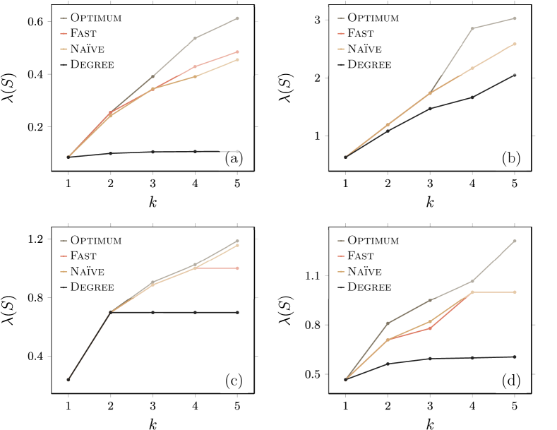
Figure 2: $\lambda(S)$ given by Fast, Naïve, Degree, and Optimum schemes for $k$ ranging from 1 to 5 on four small networks: (a) Dolphins, (b) Tribes, (c) Karate and (d) Firm-Hi-Tech.

In the above, we have shown that our algorithms Naïve and Fast exhibit similar effectiveness, which can be understood as follows. Since the difference between Naïve and Fast lies in the computation of $\lambda_{\_}S(j)=\lambda(S+j)-\lambda(S)$, the eigenvalue gap when a new node $j$ is added to set $S$. In Naïve , $\lambda_{\_}S(j)$ is directly computed by solving the eigensystem, while in Fast, $\lambda_{\_}S(j)$ is evaluated by Eq. (4). Next, we show that the two methods for calculating $\lambda_{\_}S(j)$ in algorithms Naïve and $\tilde{\lambda}_{\_}S(j)$ in Fast yield almost the same effect. To this end, we conduct experiments on four networks: Dolphins, Tribes, Karate and Email-Univ. For each network, we first randomly select five nodes forming set $S$, and then add one more node into $S$ by computing the eigenvalue gap through the methods in Naïve and Fast. Figure 3 reports the results for $\lambda_{\_}S(\cdot)$ and $\tilde{\lambda}_{\_}S(\cdot)$ for the two methods, which shows that the eigenvalue gaps returned by the two approaches are linearly proportional to each other, justifying the similarity of Naïve and Fast.

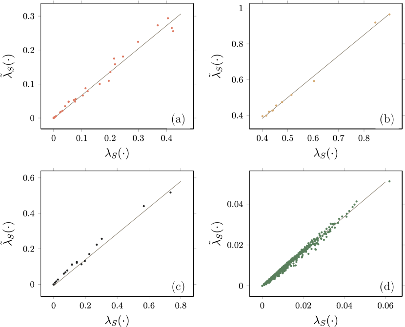
Figure 3: Eigenvalue gap returned by Naïve denoted by $\lambda_{\_}S(\cdot)$ verse eigenvalue gap returned by Fast denoted by $\tilde{\lambda}_{\_}S(\cdot)$ on four networks: (a) Dolphins, (b) Tribes, (c) Karate, and (d) Email-Univ.

We further demonstrate the efficacy of our algorithms Fast by comparing it with four baseline methods frequently used in previous work: Degree, Eigenvector, Betweenness, and Closeness on six networks, with the cardinality $k$ of set $S$ changing from $1$ to $100$. The comparison results are reported in Fig. 4, from which we can observe that our proposed algorithm Fast almost outperforms the baseline methods.

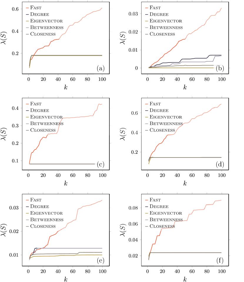
Figure 4: $\lambda(S)$ returned by Fast, Degree, Eigenvector, Betweenness, and Closeness, for $k$ ranging from 1 to 100 on six medium-size networks: (a) Pages-Government, (b) US-Grid, (c) Anybeat, (d) WHOIS, (e) Pretty Good Privacy, and (f) Epinions.

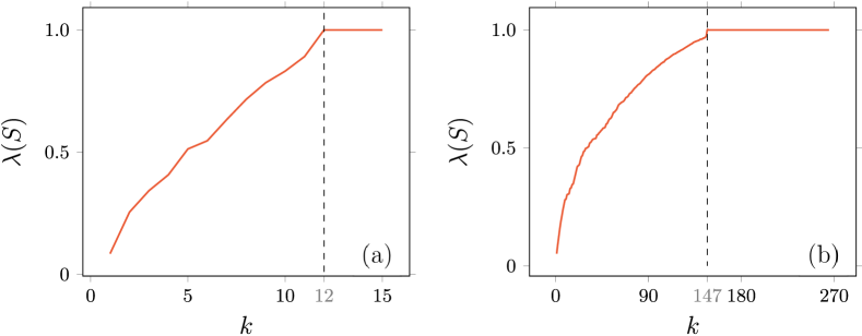
Figure 5: $\lambda(S)$ returned by Fast, on two networks: (a) Dolphins and (b) Email-Univ. The dashed line corresponds to the earliest moment when $\lambda(S)=1$ appears.

To compare with the most dominant work LiXuLuChZe21 on this optimization problem, we also repeat the experiment on Dolphins and Email-Univ in LiXuLuChZe21 . According to LiXuLuChZe21 , the Dolphins and Email-Univ’s $\lambda(S)$ are doomed to be not smaller than 1 if $S$ are their dominating sets respectively. And it takes 14 and 266 nodes for method from LiXuLuChZe21 to make $\lambda(S)$ arrive this bound. However, as shown in Fig. 5, our method only takes 12 and 147 nodes to grounded to let $\lambda(S)=1$. Besides, our method is not limited by $k$’s scale but method from LiXuLuChZe21 cannot sustain oversized $k$.

7.3 Efficiency and Scalability

Although both Fast and Naïve are very accurate, the theoretical computation complexity of the two algorithms differs greatly. Here we experimentally compare the running time of Fast and Exaxt in various real networks, which is reported in Table 2. The results show that algorithm Fast runs much faster than algorithm Naïve, especially on large-scale networks. For example, for the networks with more than 40,000 nodes marked with $*$, algorithm Naïve fails due to its tremendous time cost, while algorithm Fast takes only a few seconds for each iteration even on the network with over one million nodes, indicating the scalability of Approx to large networks.

Table 2: Average running time in one iteration for computing $\lambda_{\_}S(\cdot)$ and $C_{\_}S(\cdot)$ defined in the caption of Figure 3 and their ratio for all nodes on a larger set of real-world networks.

Network		Time (seconds)
		Exact	Approx	Ratio
685-bus		4.73	0.004	1182
Bcspwr09		22.60	0.011	2054
Routers-RF		52.15	0.046	1133
Bcspwr10		318.4	0.044	7236
Webbase-2001		2613	0.134	19500
As-Caida2007		5308	0.261	20337
Epinions		4931	0.229	21532
Email-EU		7148	0.126	56730
Internet-as*		-	0.227	-
P2P-gnutella*		-	0.482	-
RL-caida*		-	1.992	-
DBLP-2010*		-	2.141	-
Twitter-follows*		-	2.292	-
Delicious*		-	4.731	-
FourSquare*		-	16.33	-
Youtube-snap*		-	31.72	-

We also experimentally compare the two techniques, Lanzcos method and SDDM solver, for computing the eigenvector $\bm{\mathit{u}}$ associated with the smallest eigenvalue of the grounded Laplacian matrix, in terms of the computation efficiency. For this purpose, we randomly select the grounded node set $S$ with size ranging from 1 to 10, and average the time for computing eigenvector $\bm{\mathit{u}}$, as reported in Table 3. From the table, one can see that Lanzcos method is faster than SDDM solver when the networks relatively small. However, for larger networks with over 40,000 nodes, SDDM solver starts to show its advantages in terms of efficiency. For instance, for the last two networks with over 600,000 nodes, Lanzcos method fails while SDDM solver can still output the eigenvector in less than half a minute for each iteration. Thus, in all our experiments except those with results in Table 3, the eigenvector corresponding to the smallest eigenvaluewe of grounded Laplacian matrix is evaluated by SDDM solver, instead of Lanzcos method.

Table 3: Average running time for Lanzcos method and Laplaican solver for computing the eigenvector associated with the smallest eigenvalue of the grounded Laplacian matrix for some real-world networks.

Network	Time (seconds)
	Lanzcos Method	Inverse Power Method
685-bus	0.002	0.004
Bcspwr09	0.004	0.008
Routers-RF	0.011	0.016
Bcspwr10	0.013	0.033
Webbase-2001	0.020	0.102
As-Caida2007	0.116	0.193
Epinions	0.441	0.411
Email-EU	0.205	0.157
Internet-as	0.199	0.211
P2P-gnutella	4.062	0.379
RL-caida	3.081	2.034
DBLP-2010	8.390	1.157
Twitter-follows	3.328	1.371
Delicious	39.90	4.961
FourSquare	-	8.035
Youtube-snap	-	29.07

In fact, in addition to Fast, the two baseline methods Degree and Eigenvector are also scalable. As shown in Fig. 4, Degree displays the best effect among the all heuristic baseline methods, in the following, we will compare Fast with only Degree, the complexity of which is $O(n)$. Specifically, we compare Fast with Degree on four real networks with size ranging from 200,000 to 1,000,000, and report comparison results in Fig. 6. From Fig. 6, one observes that Fast outperforms Degree on all the four studied networks.

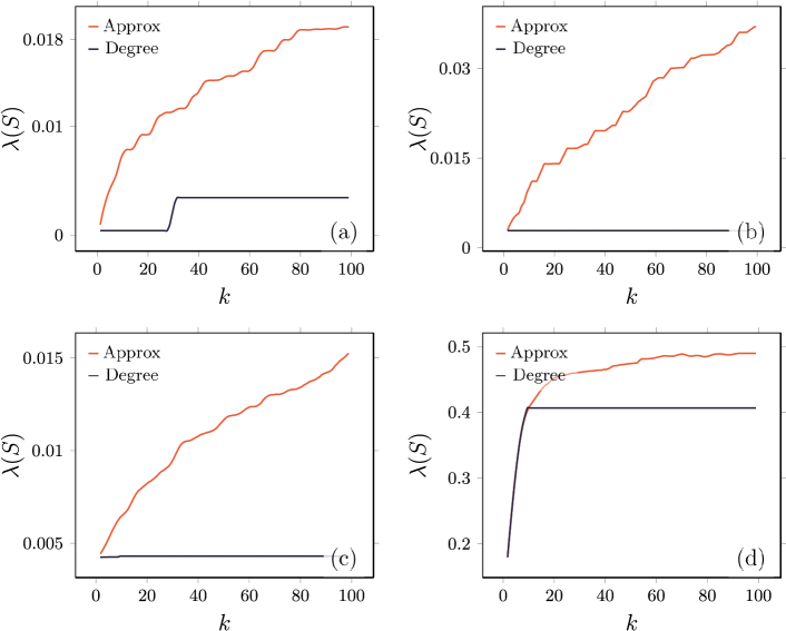
Figure 6: $\lambda(S)$ returned by Fast with Degree with $k$ ranging from 1 to 100 on four large networks: (a) RL-Caida, (b) Delicious, (c) Youtube-Snap, (d) FourSquare.

8 Conclusions

In this paper, we studied the minimum eigenvalue $\lambda(S)$ for a grounded Laplacian matrix $\bm{\mathit{L}}(S)$ of order $(n-k)\times(n-k)$, which is a principal submatrix of the Laplacian matrix $\bm{\mathit{L}}$ for a graph with $n$ nodes and $m$ edges, obtained from $\bm{\mathit{L}}$ by removing $k$ rows and columns corresponding to $k$ selected nodes forming set $S$. We focused on the problem of finding the set $S^{*}$ of $k$ nodes with an aim to maximize $\lambda(S^{*})$. This problem arises naturally in various contexts, such as maximizing the convergence speed of leader-follower consensus dynamics and maximizing the effectiveness of pinning scheme of pinning control problem. We provided a rigorous proof of the NP-hardness of this combination optimization problem, and proved that the objective function is not submodular, despite its weak strict monotonicity. We developed an approximation algorithm with time complexity $\widetilde{O}(mk)$, which maximizes $\lambda(S)$ by iteratively choosing $k$ nodes in a greedy way. Extensive experiments on various realistic networks show our algorithm is both effective and efficient, which gives almost optimal solutions and is scalable to huge networks with more than $10^{6}$ nodes.

Declarations

Availability of data and material Not applicable.

Conflict of interest There are no conflict of interest or competing interests related to this manuscript.

Acknowledgments This work was supported by the National Natural Science Foundation of China (Nos. 61872093 and U20B2051), Shanghai Municipal Science and Technology Major Project (Nos. 2018SHZDZX01 and 2021SHZDZX03), ZJ Lab, and Shanghai Center for Brain Science and Brain-Inspired Technology. Run Wang was also supported by Fudan’s Undergraduate Research Opportunities Program (FDUROP) under Grant No. 2195200241021.

References

- \bibcommenthead
- (1) Newman, M.E.J.: The structure and function of complex networks. SIAM Rev. 45(2), 167–256 (2003)
- (2) Wang, Y., Chakrabarti, D., Wang, C., Faloutsos, C.: Epidemic spreading in real networks: An eigenvalue viewpoint. In: Proc. 22nd Int. Symp. Reliab. Distrib. Syst., pp. 25–34 (2003). IEEE
- (3) Chakrabarti, D., Wang, Y., Wang, C., Leskovec, J., Faloutsos, C.: Epidemic thresholds in real networks. ACM Trans. Inf. Sys. Secur. 10(4), 1–26 (2008)
- (4) Van Mieghem, P., Omic, J., Kooij, R.: Virus spread in networks. IEEE/ACM Trans. Netw. 17(1), 1–14 (2008)
- (5) Bollobás, B., Borgs, C., Chayes, J., Riordan, O.: Percolation on dense graph sequences. Ann. Prob. 38(1), 150–183 (2010)
- (6) Olfati-Saber, R., Murray, R.M.: Consensus problems in networks of agents with switching topology and time-delays. IEEE Trans. Autom. Control 49(9), 1520–1533 (2004)
- (7) Li, H., Patterson, S., Yi, Y., Zhang, Z.: Maximizing the number of spanning trees in a connected graph. IEEE Trans. Inf. Theory 66(2), 1248–1260 (2020)
- (8) Klein, D.J., Randić, M.: Resistance distance. J. Math. Chem. 12(1), 81–95 (1993)
- (9) Li, H., Zhang, Z.: Kirchhoff index as a measure of edge centrality in weighted networks: Nearly linear time algorithms. In: Proc. 29th Ann. ACM-SIAM Symp. Disc. Alg., pp. 2377–2396 (2018)
- (10) Tetali, P.: Random walks and the effective resistance of networks. J. Theor. Probab. 4(1), 101–109 (1991)
- (11) Chandra, A.K., Raghavan, P., Ruzzo, W.L., Smolensky, R.: The electrical resistance of a graph captures its commute and cover times. In: Proc. 21st ACM Symp. Theory Comput., pp. 574–586 (1989)
- (12) Sheng, Y., Zhang, Z.: Low-mean hitting time for random walks on heterogeneous networks. IEEE Trans. Inf. Theory 65(11), 6898–6910 (2019)
- (13) Bamieh, B., Jovanovic, M.R., Mitra, P., Patterson, S.: Coherence in large-scale networks: Dimension-dependent limitations of local feedback. IEEE Trans. Autom. Control 57, 2235–2249 (2012)
- (14) Veremyev, A., Boginski, V., Pasiliao, E.L.: Analytical characterizations of some classes of optimal strongly attack-tolerant networks and their laplacian spectra. Journal of Global Optimization 61(1), 109–138 (2015)
- (15) Qi, Y., Zhang, Z., Yi, Y., Li, H.: Consensus in self-similar hierarchical graphs and Sierpiński graphs: Convergence speed, delay robustness, and coherence. IEEE Trans. Cybern. 49(2), 592–603 (2019)
- (16) Yi, Y., Zhang, Z., Patterson, S.: Scale-free loopy structure is resistant to noise in consensus dynamics in complex networks. IEEE Trans. Cybern. 50(1), 190–200 (2020)
- (17) Kammerdiner, A., Veremyev, A., Pasiliao, E.: On laplacian spectra of parametric families of closely connected networks with application to cooperative control. Journal of Global Optimization 67, 187–205 (2017)
- (18) Chen, X., Zhang, S., Zhang, L., Yu, G., Liu, J.: Determining redundant links of multiagent systems in keeping or improving consensus convergence rates. IEEE Systems Journal 16(4), 6153–6163 (2021)
- (19) Chen, X., Gao, S., Zhang, S., Zhao, Y.: On topology optimization for event-triggered consensus with triggered events reducing and convergence rate improving. IEEE Transactions on Circuits and Systems II: Express Briefs 69(3), 1223–1227 (2021)
- (20) Gorbunov, A., Peng, J.C.-H., Bialek, J.W., Vorobev, P.: Identification of stability regions in inverter-based microgrids. IEEE Transactions on Power Systems 37(4), 2613–2623 (2021)
- (21) Zhang, Y., Zhou, J., Lu, J.-a., Li, W.: Superdiffusion induced by complete structure in multiplex networks. Chaos: An Interdisciplinary Journal of Nonlinear Science 33(2), 023133 (2023)
- (22) Rahmani, A., Ji, M., Mesbahi, M., Egerstedt, M.: Controllability of multi-agent systems from a graph-theoretic perspective. SIAM J. Control Optimiz. 48(1), 162–186 (2009)
- (23) Patterson, S., Bamieh, B.: Leader selection for optimal network coherence. In: Proc. 49th IEEE Conf. Decision Control, pp. 2692–2697 (2010). IEEE
- (24) Pirani, M., Shahrivar, E.M., Fidan, B., Sundaram, S.: Robustness of leader-follower networked dynamical systems. IEEE Trans. Control Netw. Syst. 5(4), 1752–1763 (2018)
- (25) Liu, H., Xu, X., Lu, J., Chen, G., Zeng, Z.: Optimizing pinning control of complex dynamical networks based on spectral properties of grounded laplacian matrices. IEEE Trans. Syst. Man Cybern. -Syst. 51(2), 786–796 (2021)
- (26) Miekkala, U.: Graph properties for splitting with grounded Laplacian matrices. Bit 33(3), 485–495 (1993)
- (27) Barooah, P., Hespanha, J.P.: Graph effective resistance and distributed control: Spectral properties and applications. In: Proc. 45th IEEE Conf. Decision Control, pp. 3479–3485 (2006). IEEE
- (28) Wang, X.F., Chen, G.: Pinning control of scale-free dynamical networks. Physica A 310(3-4), 521–531 (2002)
- (29) Li, X., Wang, X., Chen, G.: Pinning a complex dynamical network to its equilibrium. IEEE Trans. Circuits Syst. I-Reg Papers 51(10), 2074–2087 (2004)
- (30) Herman, I., Martinec, D., Hurák, Z., Šebek, M.: Nonzero bound on fiedler eigenvalue causes exponential growth of h-infinity norm of vehicular platoon. IEEE Trans. Autom. Control 60(8), 2248–2253 (2015)
- (31) Tegling, E., Bamieh, B., Gayme, D.F.: The price of synchrony: Evaluating the resistive losses in synchronizing power networks. IEEE Trans. Control Netw. Syst. 2(3), 254–266 (2015)
- (32) Pirani, M., Sundaram, S.: Spectral properties of the grounded Laplacian matrix with applications to consensus in the presence of stubborn agents. In: 2014 Amer. Control Conf., pp. 2160–2165 (2014). IEEE
- (33) Pirani, M., Sundaram, S.: On the smallest eigenvalue of grounded Laplacian matrices. IEEE Trans. Autom. Control 61(2), 509–514 (2016)
- (34) Pirani, M., Shahrivar, E.M., Sundaram, S.: Coherence and convergence rate in networked dynamical systems. In: Proc. 54th IEEE Conf. Decision Control, pp. 968–973 (2015). IEEE
- (35) Manaffam, S., Behal, A.: Bounds on the smallest eigenvalue of a pinned Laplacian matrix. IEEE Trans. Autom. Control 63(8), 2641–2646 (2017)
- (36) Xia, W., Cao, M.: Analysis and applications of spectral properties of grounded Laplacian matrices for directed networks. Automatica 80, 10–16 (2017)
- (37) van der Grinten, A., Angriman, E., Meyerhenke, H.: Scaling up network centrality computations–A brief overview. it-Inform. Technol. 62(3-4), 189–204 (2020)
- (38) Dolev, S., Elovici, Y., Puzis, R., Zilberman, P.: Incremental deployment of network monitors based on group betweenness centrality. Inform. Proces. Lett. 109(20), 1172–1176 (2009)
- (39) Mahmoody, A., Tsourakakis, C.E., Upfal, E.: Scalable betweenness centrality maximization via sampling. In: Proc. 22nd ACM SIGKDD Int. Conf. Knowl. Discovery Data Mining, pp. 1765–1773 (2016). ACM
- (40) Everett, M.G., Borgatti, S.P.: The centrality of groups and classes. J. Math. Sociol. 23(3), 181–201 (1999)
- (41) Bergamini, E., Gonser, T., Meyerhenke, H.: Scaling up group closeness maximization. In: Proc. 12th Workshop Algorithm Engin. Experim., pp. 209–222 (2018). SIAM
- (42) Li, H., Peng, R., Shan, L., Yi, Y., Zhang, Z.: Current flow group closeness centrality for complex networks? In: Proc. World Wide Web Conf., pp. 961–971 (2019)
- (43) Ghosh, R., Teng, S.-h., Lerman, K., Yan, X.: The interplay between dynamics and networks: centrality, communities, and cheeger inequality. In: Proc. 20th ACM SIGKDD Int. Conf. Knowl. Discovery Data Mining, pp. 1406–1415 (2014). ACM
- (44) Wang, B., Liu, H., Xu, J., Liu, J.: Pining control algorithm for complex networks. In: Proc. 2019 Chin. Control Conf., pp. 964–969 (2019). IEEE
- (45) Clark, A., Alomair, B., Bushnell, L., Poovendran, R.: Leader selection in multi-agent systems for smooth convergence via fast mixing. In: Proc. 51st IEEE Conf. Decision Control, pp. 818–824 (2012). IEEE
- (46) Clark, A., Bushnell, L., Poovendran, R.: Leader selection for minimizing convergence error in leader-follower systems: A supermodular optimization approach. In: Proc. 10th Int. Symp. Model. Optimiz. Mobile, Ad Hoc and Wirel. Netw., pp. 111–115 (2012). IEEE
- (47) Clark, A., Hou, Q., Bushnell, L., Poovendran, R.: Maximizing the smallest eigenvalue of a symmetric matrix: A submodular optimization approach. Automatica 95, 446–454 (2018)
- (48) Zhou, J., Tang, W.K.: Feature-embedded evolutionary algorithm for network optimization. In: Proc. 2020 IEEE Int. Symp. Circuits Syst., pp. 1–5 (2020). IEEE
- (49) McDonald, J.J., Neumann, M., Schneider, H., Tsatsomeros, M.J.: Inverse M-matrix inequalities and generalized ultrametric matrices. Linear Algebra Appl. 220, 321–341 (1995)
- (50) MacCluer, C.R.: The many proofs and applications of Perron’s theorem. SIAM Rev. 42(3), 487–498 (2000)
- (51) Nemhauser, G.L., Wolsey, L.A., Fisher, M.L.: An analysis of approximations for maximizing submodular set functions-I. Math. Program. 14(1), 265–294 (1978)
- (52) Fricke, G., Hedetniemi, S.T., Jacobs, D.P.: Independence and irredundance in -regular graphs. Ars Comb. 49, 271–279 (1998)
- (53) Bapat, R.B.: Graphs and Matrices. New York: Springer, ??? (2010)
- (54) Lanczos, C.: Solution of systems of linear equations by minimized iterations1. J. Res. Natl. Inst. Bereau Stand. 49(1) (1952)
- (55) Chaiken, S.: A combinatorial proof of the all minors matrix tree theorem. SIAM J. Alg. Discrete Met. 3(3), 319–329 (1982)
- (56) Yi, Y., Shan, L., Li, H., Zhang, Z.: Biharmonic distance related centrality for edges in weighted networks. In: Proc. 27th Int. Joint Conf. Art. Intel., pp. 3620–3626 (2018)
- (57) Siami, M., Bolouki, S., Bamieh, B., Motee, N.: Centrality measures in linear consensus networks with structured network uncertainties. IEEE Trans. Control Netw. Syst. 5(3), 924–934 (2018)
- (58) Kang, J., Tong, H.: N2N: network derivative mining. In: Proceedings of the 28th ACM Int. Conf. Inf. Knowledge Manage., CIKM 2019, Beijing, China, November 3-7, 2019, pp. 861–870. ACM, ??? (2019)
- (59) Mieghem, P.: Graph Spectra for Complex Networks. Cambridge University Press, ??? (2011)
- (60) He, Z., Yao, C., Yu, J., Zhan, M.: Perturbation analysis and comparison of network synchronization methods. Phys. Rev. E 99 (2019)
- (61) Milanese, A., Sun, J., Nishikawa, T.: Approximating spectral impact of structural perturbations in large networks. Phys. Rev. E 81 (2010)
- (62) Restrepo, J.G., Ott, E., Hunt, B.R.: Characterizing the dynamical importance of network nodes and links. Phys. Rev. Lett. 97 (2006)
- (63) Bocea, M., Panagiotopoulos, P.D., Rădulescu, V.: A perturbation result for a double eigenvalue hemivariational inequality with constraints and applications. Journal of Global Optimization 14, 137–156 (1999)
- (64) Batson, J., Spielman, D.A., Srivastava, N., Teng, S.H.: Spectral sparsification of graphs: Theory and algorithms. Commun. ACM 56(8), 87–94 (2013)
- (65) Spielman, D.A., Teng, S.-H.: Nearly linear time algorithms for preconditioning and solving symmetric, diagonally dominant linear systems. SIAM J. Matrix Anal. Appl. 35(3), 835–885 (2014)
- (66) Cohen, M.B., Kyng, R., Miller, G.L., Pachocki, J.W., Peng, R., Rao, A.B., Xu, S.C.: Solving SDD linear systems in nearly time. In: Proc. 46th Annu. ACM Symp. Theory Comput., pp. 343–352 (2014). ACM
- (67) Kunegis, J.: Konect: the koblenz network collection. In: Proc. 22nd Int. Conf. World Wide Web, pp. 1343–1350 (2013). ACM
- (68) Leskovec, J., Sosič, R.: SNAP: A general-purpose network analysis and graph-mining library. ACM Trans. Intel. Syst. Tech. 8(1), 1 (2016)