Resolution Exchange with Tunneling
for Enhanced Sampling of Protein Landscapes

Abstract

Simulations of protein folding and protein association happen on timescales that are orders of magnitude larger than what can typically be covered in all-atom molecular dynamics simulations. Use of low-resolution models alleviates this problem but may reduce the accuracy of the simulations. We introduce a replica-exchange-based multiscale sampling technique that combines the faster sampling in coarse-grained simulations with the potentially higher accuracy of all-atom simulations. After testing the efficiency of our Resolution Exchange with Tunneling (ResET) in simulations of the Trp-cage protein, an often used model to evaluate sampling techniques in protein simulations, we use our approach to compare the landscape of wild type and A2T mutant A$\beta_{1-42}$ peptides. Our results suggest a mechanism by that the mutation of a small hydrophobic Alanine (A) into a bulky polar Threonine (T) may interfere with the self-assembly of A$\beta$-fibrils.

I Introduction

While molecular dynamics is now commonly used to study folding, association and aggregation of proteins and other biological macromolecules [1, 2, 3, 4, 5, 6, 7, 8, 9], biochemical processes such as the formation of amyloid fibers from monomers [9, 5, 10] often occur on timescales [11, 10] that exceeds what can be covered in all-atom simulations. Coarse-graining, i.e., lowering the resolution of a system [12, 4, 13, 14, 15, 16], allows one to reduce the computational difficulties and to access timescales not obtainable to the fine-grained all-atom models [4, 12], but it often results in lower accuracy. This is because the smaller number of degrees of freedom lowers the entropy of the system, and it is difficult to compensate for this reduction by modifying the enthalpic contributions accordingly [12]. Multiscale techniques try to combine the advantages of fine-grained models (that are more accurate but costly to evaluate) with that of coarse-grained models (which are less detailed but enable larger time steps).

One example is Resolution Exchange [17] where the replica-exchange protocol [18] is used to induce a walk in resolution space. In the same way that for Replica-Exchange molecular dynamics (REMD) [18, 19] the walk in temperature space leads to faster sampling at low temperatures, enables exploration of resolution space a faster convergence of simulations at an all-atom level [17, 20]. However, the replica-exchange step requires reconstruction of the fine-grained degrees of freedom of a previously coarse-grained configuration, for instance, by adding side chains to a conformation that was described prior only by the backbone. Various approaches [21, 22, 23, 17, 20] have been developed to address this problem, but often they result in high energies of the proposal configuration (and therefore low acceptance rates) [20, 21] or introduce biases [22, 23].

The dilemma can be alleviated by introducing a potential energy made of three terms:

$$E_{pot}=E_{FG}+E_{CG}+\lambda E_{\lambda}~{}.$$ (1)

The first term is the energy $E_{FG}$ of the protein system and the surrounding environment as described by an all-atom (fine-grained) model. The second term $E_{CG}$ describes the same system by a suitable coarse-grained model. Both models are coupled by a system-specific penalty term $E_{\lambda}$ [24, 25] that measures the similarity between the configurations at both levels of resolution, with the strength of coupling controlled by a replica-specific parameter $\lambda$. Hence, Hamilton Replica Exchange [26, 27] of the above defined multiscale system leads to an exchange of information between fine-grained and coarse-grained models, with measurements taken at the replica where $\lambda=0$. However, while avoiding the problem of steric clashes in resolution exchange, the exchange probability is often still small [28], and the resulting need to use multiple replica to bridge the two levels of resolution makes this approach not appealing.

As an alternative, we propose here a Resolution Exchange with Tunneling (ResET) approach that requires only two replicas. Working and efficiency of our approach is tested in simulations of the Trp-cage [29, 30] miniprotein (Protein Data Bank (PDB) Identifier: 1L2Y), an often used model for testing new sampling techniques. As a first application we use in the second part ResET to compare the landscape of A$\beta_{1-42}$ wild type peptides, implicated in Alzheimer’s disease, with that of A2T mutants which seems to protect against Alzheimer’s disease [31, 32, 33]. Our results suggest a mechanism by that the mutation of a small hydrophobic Alanine (A) into a bulky polar Threonine (T) may interfere with the self-assembly of A$\beta$-fibrils, decreasing the chance for formation of the A$\beta$-amyloids that are a hallmark of Alzheimer’s disease  [34, 35, 36].

II Resolution Exchange with Tunneling

Resolution Exchange with Tunneling (ResET) utilizes two replica, each containing both a coarse-grained and a fine-grained representation of the system. On each replica, both representations evolve separately by molecular dynamics. On the first replica, A, is the coarse-grained model in a configuration $A_{CG}$ and has a potential energy $E^{pot}_{CG}(A_{CG})$ and a kinetic energy $E^{kin}_{CG}(A_{CG})$. On the other hand, the fine-grained model is in a configuration $A_{FG}$ that has a kinetic energy $E^{kin}_{FG}(A_{FG})$ and a potential energy $E^{biased}_{FG}(A_{FG})$ which depends on the configuration $A_{CG}$ of the coarse-grained model by $E^{biased}_{FG}(A_{FG})=E^{pot}_{FG}(A_{FG})+\lambda_{1}E_{\lambda}(A_{CG},A_{FG})$. Hence, the two models on this replica interact only by the term $\lambda_{1}E_{\lambda}(A_{CG},A_{FG})$ that biases the fine-grained model, but are otherwise invisible to each other. The effect of this biasing term is that configurations of the fine-grained model are favored which resemble the coarse-grained model configuration, with the strength of the bias controlled by parameter $\lambda_{1}$. The opposite situation is found on the replica B. Here lives an independent fine-grained model with configuration $B_{FG}$ that has a potential energy $E^{pot}_{FG}(B_{FG})$ and kinetic energy $E^{kin}_{FG}(B_{FG})$, while, on the other hand, the configuration $B_{CG}$ of the coarse-grained model has a kinetic energy $E^{kin}_{CG}(B_{CG})$ and a potential energy $E^{biased}_{CG}(B_{FG},B_{CG})=E^{pot}_{CG}(B_{BG})+\lambda_{2}E_{\lambda}(B_{CG},B_{FG})$ that depends on the fine-grained model by a term $\lambda_{1}E_{\lambda}(A_{CG},A_{FG})$. This biasing term now ensures that on replica B the coarse-grained configuration resembles the one of the fine-grained model.

While the time step for integrating fine-grained and coarse-grained models may differ, they have to be the same for the corresponding models on both replicas. This is because after a certain number of molecular dynamics steps a decision is made on whether to replace on the replica B the configuration $B_{FG}$ in the unbiased fine-grained model by the configuration $A_{FG}$ of the auxiliary (biased) fine-grained model of the replica A. This replacement goes together with a re-weighting of the velocities $v_{FG}(A_{FG})$ such that $\hat{E}^{kin}_{FG}(A_{FG})=E^{kin}_{FG}(B_{FG})$, and is accepted with probability:

$$w(B\rightarrow A)=\min\left(1,\exp(-\beta(E^{pot}_{FG}(A_{FG})-E^{pot}_{FG}(B_{BG})-\lambda_{1}E_{\lambda}(A_{FG},A_{CG})-\Delta E^{kin}_{FG})\right)$$ (2)

with $\Delta E^{kin}_{FG}=E^{kin}_{FG}(A_{FG})-E^{kin}_{FG}(B_{FG})$. The re-weighting of the velocities and the Metropolis-Hastings acceptance criterium accounts for the fact that the proposal configurations $A_{FG}$ are generated on replica A by a biased process, i.e., it corrects for the resulting skewed probability with which the configuration $A_{FG}$ is proposed as a replacement for $B_{FG}$.

At other times, the the coarse-grained configuration $A_{CG}$ on replica A is replaced by the configuration $B_{CG}$ of the biased coarse-grained model on replica B with probability:

$$w(A\rightarrow B)=\min\left(1,\exp(-\beta(E^{pot}_{CG}(B_{CG})-E^{pot}_{CG}(A_{BG})-\lambda_{2}E_{\lambda}(B_{FG},B_{CG})-\Delta E^{kin}_{CG})\right)$$ (3)

with $\Delta E^{kin}_{CG}=E^{kin}_{CG}(B_{CG})+E^{kin}_{CG}(A_{CG})$. Re-weighting the velocities of configuration $B_{CG}$ such that $\hat{E}^{kin}_{CG}(B_{CG})=E^{kin}_{CG}(A_{CG})$, and the Metropolis-Hastings acceptance criterium are again to correct for the skewed probability by which the configuration $B_{CG}$ is proposed.

Note that the update of the unbiased coarse-grained configuration on replica A also changes the $E_{\lambda}$ biasing term in the ancillary fine-grained configuration, as does the update of the unbiased fine-grained configuration on replica B changes the corresponding biasing term in the steered coarse-grained configuration. In order to minimize this disturbance, we also rescale the velocities in the biased models such that the change in kinetic energy compensates for the change in $E_{\lambda}$.

We remark that in software packages such as GROMACS [37] it is sometimes simpler to separate the biased and unbiased models onto different replicas. In this case one would have four replicas, with a possible distribution of the models sketched in the table below.

Model	replica	Potential Energy	Kinetic Energy	Lambda	Lambda Energy
unbiased fine-grained model	0	$P_{0}$	$K_{0}$
biased fine-grained model	1	$P_{1}$	$K_{1}$	$\lambda_{1}$	$E_{\lambda}(1,3)$
biased coarse-grained model	2	$P_{2}$	$K_{2}$	$\lambda_{2}$	$E_{\lambda}(0,2)$
unbiased coarse-grained model	3	$P_{3}$	$K_{3}$

In this implementation, the replica 0 and 2, and replica 1 and 3, communicated during the molecular dynamics evolution of the configurations; and the ResET move replaces the configuration of replica 0 by that of replica 1, and/or the configuration on replica 3 by that of replica 2.

III Materials and Metods

III.1 Set up of the ResET simulations

Our simulations utilize a modified version of the GROMACS [37] molecular package available from the authors. Initial tests of the working and efficiency are for the Trp-cage protein [29, 30], an often used system for evaluating new algorithms. In order to compare our simulations with previous studies, we follow closely the set-up of Han et al [38] for the coarse-grained model, and that of Kouza et al [39] for the fine-grained model. Hence, our coarse-grained Trp-cage protein model is described by PACE force-field [4], with the uncapped protein solvated by 1118 MARTINI [40] coarse-grained water molecules, and buffered 0.15M $Na^{+}$ and $Cl^{-}$ ions, in a cubic box of length 5.18 nm, leading to a total of 1313 coarse-grained particles. On the other hand, in our fine grained model is the N-terminus capped by an acetyl group and at C-terminus by methylamine, leading to a total number of 313 atoms for the protein that are solvated with 2645 extended simple point charge (SPC/E [41]) water molecules in a cubic box with an edge length of 4.4 nm. One chlorine ion ($Cl^{-}$) is added to neutralize the system. Hence, the system contains 8249 fine-grained particles, with the interactions between them described by the AMBER94 force-field [42].

As a first application we compare in the second part of this study the ensemble of configurations sampled by ResET simulation of A$\beta_{1-42}$ wild type and A2T mutant peptides. While aggregates of the wild type A$\beta$-peptides are implicated in Alzheimer’s disease, the A2T mutant appears to be protective, i.e, reducing the probability for acquiring the disease. We use in our simulations for both wild type and mutant as coarse-grained model the MARTINI force-field [40], which is computationally efficient and has been already used earlier in A$\beta$ simulations [43, 44]. Here, the main chain of each amino acid is represented by one bead, and the side chains by up to four beads depending on the size of the amino acid. Our wild type protein thus contains 91 beads, and the mutant 92 beads. Each peptide is placed in a cubic box and solvated with the MARTINI-CG water molecules represented by single beads. Together with 3 $Na^{+}$ MARTINI-ion beads and a box size of 7.16 nm (wild type) and 7.24 nm A2T mutant) we arrive at 2925 and 3189 particles, respectively. On the other hand, the fine-grained representations of wild type and mutant peptides are modeled by the CHARMM36 force-field [45] which we found in previous work to be efficient for simulations of intrinsically disordered and amyloid-forming proteins. The N- and C-termini are capped with Methyl groups. The protein is placed in the center of a cubic box using a 1 nm distance between the atoms of the protein and box. The each system is solvated with TIP3 water molecules [46] and neutralized with 3 $Na^{+}$ ions. This leads to a box size of 7.5 nm and a total number of 41412 particles for the wild type. Correspondingly, we get a box size of 7.6nm and a total number of 44509 particles for the mutant.

In simulations of both the Trp-cage protein and the A$\beta$-peptides we use for both fine-grained and coarse-grained models shift functions with a cut-off of 1.2 nm in the calculations of Coulomb and van der Waals interactions. Because of periodic boundary conditions we employe Particle mesh Ewald (PME) [47] summation to account for long-range electrostatic interactions. Hydrogen atoms and bond distances are constraint in the fine-grained model by the LINCS algorithm [48]. Equations of motion are integrated using a leap-frog algorithm, with a time step of 2 fs for both the fine-grained model and coarse-grained model. The v-rescale thermostat  [49] with a coupling time of 0.01 ps is used to maintain the temperature in the coarse-grained models, while a Nose-Hoover [50, 51] thermostat with the coupling time of 0.5 ps controls the temperature in the fine-grained models.

A key element of the ResET sampling technique is the restraining potential $E_{\lambda}$ which quantifies the similarity between fine-grained and coarse-grained configurations. In our case, we choose a function of the form [25].

$$E_{\lambda}(q_{FG},q_{CG})=\left\{\begin{array}[]{ll}{\displaystyle\frac{1}{2}\left(\Delta^{2}\left(i,j\right)\right)}&-ds<\Delta\left(i,j\right)<ds\\ {\displaystyle A+\frac{B}{\Delta^{S}\left(i,j\right)}+f_{max}\Delta(i,j)}&\Delta(i,j)>ds\\ {\displaystyle A+\frac{B}{\Delta^{S}(i,j)}\left(-1\right)^{S}-f_{max}\Delta(i,j)}&\Delta(i,j)<-ds\end{array}\right.$$ (4)

where $q_{FG}$ are the coordinates of atoms in the fine-grained model and $q_{CG}$ the ones in the coarse-grained model. $\Delta(ij)=\delta_{FG}(ij)-\delta_{CG}(ij)$ is the difference between the distances ($\delta(ij)$) measured in either the fine-grained or the coarse-grained models between the C_α-atoms i and j. The control parameter $f_{max}$ sets the maximum force as $\Delta\left(i,j\right)\rightarrow\infty$ and $S$ determines how fast this value is realized. The parameters $A$ and $B$ are included to ensure continuity of $E_{\alpha}(q_{fg},q_{cg})$ and it’s first derivative at values where $\Delta\left(i,j\right)=\pm ds$, i.e., where the functional form of 4 changes. These parameters are thus computed by

$$A=\left(\frac{1}{2}+\frac{1}{S}\right)ds^{2}-\left(\frac{1}{S}+1\right)f_{max}ds\quad and\quad B=\left(\frac{f_{max}-ds}{S}\right)ds^{S+1}.$$ (5)

In the ResET simulations is the biased fine-grained model on replica A coupled to the unbiased coarse-grained model by a parameter $\lambda_{1}=0.5$, while on replica B the biased coarse-grained models is coupled to the free fine-grained models by a parameter $\lambda_{2}=2.5$. The ResET replacement move is tried every 250 ps, with the bias-correction factor $\lambda_{1}E_{\lambda}(A_{FG},A_{CG})-\Delta E^{kin}_{FG}$ limited to the interval (0,100), and on replica B $\lambda_{2}E_{\lambda}(B_{FG},B_{CG})-\Delta E^{kin}_{CG})$ to the interval (0,20), choices that we found in preliminary test runs leading to increased numerical stability.

Table 1: Simulation details

		Trp-cage				A$\beta_{1-42}$
Method	Force-Field	Sampling No	Time (ns)		Force-Field	Sampling No	Time(ns)
Canonical FG	AMBER94	3	5000		CHARMM36	$---$	$---$
REMD FG	AMBER94	1	200		$---$	$---$	$---$
ResET FG+CG	AMBER94+PACE	6	200(1000)		CHARMM36+MARTINI v2.2	2	100(500)

Start structures for both fine-grained and coarse-grained models are generated by heating up the experimental structures of PDB-ID: 1L2Y (Trp-cage) and PDB-ID: 1Z0Q (A$\beta_{1-42}$) [52, 34] to 500 or 1000 K in short molecular dynamics simulations under NVT conditions (0.5 ns and 1 ns), and cooling them down to the respective temperatures (with the exception of the REMD simulations is this 310 K). Simulations of the various systems start from the so-generated configurations and are performed in the NVT ensemble, with the simulation details listed in Table 1.

For most of our analysis we use GROMACS tools [37] such as gmx-rms which calculates the root-mean-square deviation (RMSD) and the root-mean-square fluctuations (RMSF) of residues with respect to an initial configuration. For visualization we use the VMD software [53], which we also use to calculate the solvent accessible surface area (SASA) using a probe radius of 1.4 Å. Other quantities are calculated with in-house programs and defined in the manuscript. An example are dynamic cross-correlation maps which are calculated using the definition of [54, 55]:

$$C(i,j)=\frac{\langle\Delta{\bf r}_{i}.\Delta{\bf r}_{j}\rangle}{\langle\Delta{\bf r}_{i}^{2}\rangle\langle\Delta{\bf r}_{j}^{2}\rangle}.$$ (6)

where $\Delta{\bf r}_{i}$ and $\Delta{\bf r}_{i}$ are the displacement vectors of $i$-th and $j$-th residues of the system and angle brackets represent ensemble averages. Positive values mark correlated motions of the respective residues while negative values indicate anti-correlated motion.

IV Results and Discussion

IV.1 Efficiency of ResET

In order to test the working and efficiency of our multiscale approach ResET, we perform first simulations of the Trp-cage [29, 30] miniprotein, an often used model for testing sampling techniques. Choice of this system, with which we are familiar from previous work, therefore allows a direct comparison with past simulations. An example are the replica exchange molecular dynamics (REMD) simulations of Ref. [56, 39], where 40 replicas of equal volume are simulated at 40 temperatures spanning a range from T= 280 K to T=540 K. Configurations are exchanged between neighboring temperatures according to a generalized Metropolis criterium, leading to a random walk in temperature that allows replicas to find local minima (when at low temperatures) and escape out of them (when at high temperatures). The net-effect is an enhanced sampling at the target temperature. Defining a configuration as native-like if the root-mean-square deviation (RMSD) to the PDB-structure (PDB-ID: 1L2Y) of less than 2.5 Å, we find at T=310 K native-like configuration with a frequency of 87 %, using the more restrictive criterium of a RMSD smaller than 2.2 Å, the frequency reduces to 55%. Note, that these frequencies do not change beyond statistical fluctuations once the REMD simulation has reached 50 ns, and we therefore neglect the first 50 ns of our 200 ns long trajectories when calculating the frequencies. While these frequencies are similar to the ones observed in earlier work [56, 39], we suspect that our values overestimate the frequency of folded configurations that reside at a certain time at T=310 K. This is because the systems are simulated at each temperature with the same volume. This volume, while sufficiently large at the target temperature may at the higher temperature suppress extended configurations, therefore artificially stabilizing folded configurations. For this reason, we prefer to compare our ResET simulations instead directly with regular constant temperature molecular dynamics, simulating the Trp-cage protein in three independent trajectories at T=310 K over 5000 ns, a value that is comparable to the experimental measured folding times of around 4$\mu$  [57]. The RMSD as function of time is shown for all three trajectories in Figure 1a.

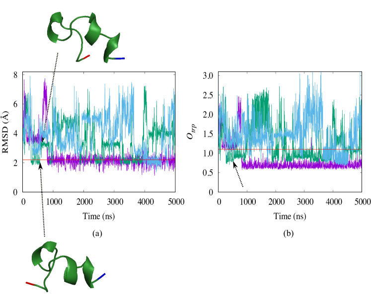
Figure 1: The time evolution of RMSD (a) and folding parameter $O_{trp}$ (b) as measured in regular molecular dynamics simulations at T=310 K. Trajectory 1 is drawn in purple, trajectory 2 in green and trajectory 3 in blue. The two snapshots are taken from trajectory 2 at 601.0 ns (snapshot at the bottom) and 602.3 ns (snapshot on top). Both snapshots show similar configurations while the RMSD changes from 2.0 Å  to 3.6 Å. N- and C-terminal residues in the snapshots are marked in blue and red color, respectively.

Visual inspection of the three trajectories points to another problem. For a small protein such as Trp-cage is the RMSD not good measure for similarity as configurations that appear as similar by visual inspection may differ by relatively large RMSD values. This can be seen, for instance, in the second trajectory where at around 600 ns the RMSD increases from 2.0 Å  to 3.6 Å, i.e., from native-like to configurations to one considered no longer native-like according to the above definition of a native configuration (i.e., having a RMSD of less than 2.5 Å). However, visual inspection shows that the molecule keeps its native-like fold, see the corresponding configurations also shown in the Figure. This contradiction between our RMSD-based definition and visual inspection made us configurations while the RMSD consider another quantity as measure for similarity. The two main characteristics of the Trp-cage native structure are its two helices (residues 2-9 and 11-14), and the contact between residues 6W (a Tryptophan) and residue 18P (a Proline). Hence we define as marker for Trp-cage folding a new quantity:

$$O_{trp}=d_{6-18}+1/(n_{H}+1)$$ (7)

Here, $d_{6-18}$ is the difference between residues 6W and 18P, and $n_{H}$ the number of residues that have dihedral angles as seen in a helix. The time evolution of this quantity in Figure 1b shows that the new coordinate allows indeed a better description of the folding transitions, as its behavior differs less from the visual inspection. Especially, we do not see for the second trajectory at 600 ns the false signal for non-native configurations that we see in the RMSD plot. Comparing $O_{trp}$ as function of time with visual inspection of configurations along the trajectories suggests that folded configurations are characterized by values of $O_{trp}<1$, and we use in the following this definition to quantify frequencies of folded configurations.

With this definition, we observe the first folding event at t=11.6 ns (in trajectory 2), and the systems stays folded for about 600 ns before unfolding again. For trajectory 1 folding is observed at t=800 ns, and no folding is observed within 3500 ns in the third trajectory where the protein unfolds afterwards again at about 4500 ns. As a consequence, we find between 250 ns and 500 ns folded configurations with a frequency of about 26% and between 750 ns and 1000 ns, with about 49%. The frequencies increase only slowly as the simulations proceed, and between 3000 ns and 5000 ns we find native-like configurations with about 58%. The above numbers are consistent with the experimentally measured folding times of about 4$\mu$  [57].

How does our new multiscale method fits in this discussion? The time evolution of our marker function $O_{trp}(t)$ is shown in Figure 2. Native-like configurations according to our criterium are observed after around 30 ns, and between 50 ns and 100 ns seen with a frequency of about 59%. The frequencies do not change much as the simulation progresses, and between 150 ns and 200 ns are native-like configurations observed with 65%. We remark that these frequencies do not depend on the choice of parameters with which we scale the $\lambda$ energy contribution in the ResET update.

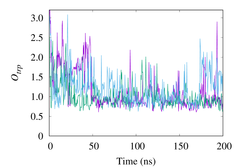
Figure 2: The time evolution of the order parameter for 100-20 kJ/mol. Trajectory 1 is drawn in purple, trajectory 2 in green and trajectory 3 in blue.

These frequencies for folded configurations are similar to what is seen in long-time canonical runs, but require shorter simulation times. Hence, our simulations of the Trp-cage protein indicate that our new multiscale simulation method leads indeed to an increase in sampling efficiency. If we take as criterium for the comparison the time it takes to have (on average) about 50% of configuration folded (about 800 ns for the canonical runs and 50 ns for the ResET run) we find that ResET is about 16 times faster than the canonical simulations. While the gain in efficiency will depend on the specifics of the coarse-grained model (i.e. how much faster it samples the configuration space) and its coupling to the physical force-field, our data demonstrate the faster sampling properties of our multiscale approach.

IV.2 Comparing A$\beta$ wild type and A2T mutant

Our evaluation of the sampling efficiency of ResET relies on a rather simple test case. As a more interesting first application, we use in the second part our sampling technique to compare the ensembles of wild type and A2T mutant A$\beta_{1-42}$ peptides. Fibrils containing A$\beta_{1-40}$ or the more toxic A$\beta_{1-42}$ are a hallmark of Alzheimer’s disease and the focus of intense research [31]. A large number of familial mutations are known that worsens the symptoms of Alzheimer’s disease or hasten its outbreak [32, 33], but there have been also mutations identified that are protective, i.e. lower the risk to fall ill with Alzheimer’s disease. One example is the mutant A2T where the second residue (counted from the N-terminus) is changed from a small hydrophobic Alanine (A) into a bulky polar Threonine (T) [34]. It has been not yet established why this mutation is protective [35, 36], but one possibility is that this mutation alters the pathway for amyloid formation, for instance, by making it more difficult to form aggregates. In order to test this hypothesis we simulate here A$\beta_{1-42}$ wild type and A2T mutant monomers, and compare the ensembles of sampled configurations for their aggregation propensities.

Under physiological conditions are A$\beta$-peptides intrinsically disordered, and we do not expect the appearance of folded structures. Instead, we assume that the ensemble of configurations contains such with transiently formed $\beta$-strands that would encourage aggregation. We conjecture that such transient ordering appears more often for wild type A$\beta_{1-42}$ than for the A2T mutant peptides. In order to identify these differences in local ordering, we have measured the root-mean-square-fluctuations (RMSF) of residues for both cases, taking as reference structure the corresponding start configuration, but discarding for the calculation of the RMSF the first 50 ns of the simulation. The RMSF is chosen because this quantity describes the flexibility of residues or segments of the protein, and the more flexible a segment is the less likely will it be involved in forming stable structures. Our data are shown in Figure 3, and while there are only small differences for the first 20 residues between wild type and mutant, the situation is different for the C-terminal half of the chain. For residues 21-37 is the RMSF considerably lower for the mutant than for the wild type. We remark that this picture does not change if we recalculate the RMSF, including now all heavy atoms (i.e, not only backbone but also side-chain atoms).

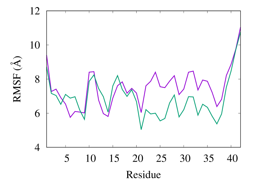
Figure 3: Root-mean-square-fluctuations of residues in either wild type (purple) or A2T mutant (green) A$\beta_{1-42}$ peptides. Only heavy atoms are considered in the calculation, and the first 50 ns of the 100 ns trajectories discarded to allow for convergence of the simulations.

The lower flexibility of the segment 21-37 in the mutant is not correlated with increased secondary structure. Residues take dihedral angle values as in a helix or a $\beta$ strand with about 10% in both wild type and mutant. However, there is a change in the average radius of gyration (RGY, a measure for the volume), which with 10.6(1) Å is larger for the mutant than for the wild type where it is 10.5(1) Å. Similarly is the average solvent accessible surface area (SASA) of the peptide in the mutant with 38.0(1) nm² less fluctuating than in the wild type (38.0(3) nm²), reflecting the gain in surface area resulting from the more bulky Threonine. However, the relation is different for the segment of residues 21-37, where the wild type has a SASA value of 18.2(3) nm² and the mutant a SASA of 18.1(2) nm² . The differences for the segment result from polar residues as the solvent accessible surface area of hydrophobic residues is with 4.1(1) nm² the same for both mutant and wild type. Hence, the differences in SASA values for this segment indicate that in the mutant polar residues, which are exposed to solvent in the wild type, form contacts with other residues. In order to understand the differences between mutant and wild type in more detail, we have also analyzed the contacts and cross-correlations between residues, focusing again on the final 50 ns of the trajectories for both systems. The resulting maps for both systems are shown in Figure 4 a-b, with the coloring describing the degree of correlation between residues.

Unlike in the wild type are in the A2T mutant the disordered N-terminus (residues 1-9) and residues 27-33 correlated. This correlation results from electrostatic interactions, for instance between the NH3+ group of residue K28 (a Lysin) with negatively-charged COO- group of residue E7 (a Glutamic acid) seen in the snapshot shown in Figure 4 d. Hence, the replacement of the small hydrophobic Alanine by a bulky polar Threonine allows for the above electrostatic interactions in the mutant that do not exist in the wild type, and whose importance for inhibiting amyloid formation in the A2T mutant has been already noticed earlier in Ref.[58]. These interactions likely stabilize not only the segment 27-33, but are responsible for the lower RMSF seen for residues 21-37. The interactions between N-terminus and residues 27-33 compete now in the A2T with hydrophobic interactions between the segment formed by residues 13-21, which include the central hydrophobic core (L₁₇VFFA₂₁), and the mostly hydrophobic C-terminus (residues 37-42), see the corresponding snapshot in Figure 4 c. As a result the two segments are correlated in the wild type but not in the mutants. These interactions between the peptide’s two main hydrophobic domains are thought to be crucial for the self-assembly of A$\beta$-fibrils [59, 60], but are now missing in the A2T mutant, reducing the risk for aggregation.

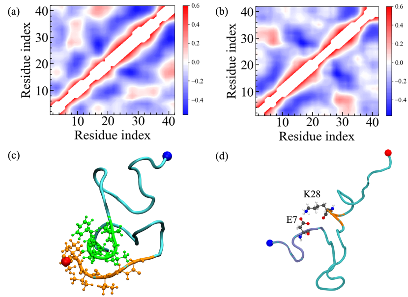
Figure 4: Two-dimensional dynamic cross-correlation map extracted from (a) wild type and (b) mutant A$\beta_{1-42}$ ResET simulations. A representative snapshot obtained from the wild type simulations is shown in (c), where the central hydrophobic core L₁₇VFFA₂₁ and the C-terminal hydrophobic residues G₃₇GVVIA₄₂ are drawn in green and orange color, respectively. A corresponding snapshot from the mutant simulation is shown in (d), where the disordered N-terminus (residues 1-10) and residues 27-31 are colored in ice-blue and orange, respectively. N- and C-terminal residues are represented by blue and red spheres.

V Conclusions

We have described a replica-exchange-based multiscale simulation method, Resolution-Exchange with Tunneling (ResET), designed for simulation of protein-folding and aggregation. Our approach combines the faster sampling in coarse-grained simulations with the potentially higher accuracy of all-atom simulations. It avoids the problem of low acceptance rates plaguing similar approaches and requires only few replica. After testing the accuracy and efficiency of our approach for the small Trp-cage protein by comparing our approach with long-scale (5 $\mu$s) regular molecular dynamic simulations, we use our new method to compare to compare the ensemble of A$\beta_{1-42}$ wild type peptides, implicated in Alzheimer’s disease, with that of A2T mutants which seems to protect against Alzheimer’s disease. Our ResET simulations indicate that the replacement of a small Alanine (A) by a bulky Threonine (T) as residue 2 alters the pathway for amyloid formation by introducing steric constraints on the mostly polar N-terminal residues that encourage electrostatic interactions with residues 27-33. These interactions reduce the flexibility of the extended segment 21-37, therefore contributing to the overall larger volume, more exposed surface and resulting higher solubility of the mutant. At the same time do this interactions also interfere with the hydrophobic interactions between the central hydrophobic core (L₁₇VFFA₂₁), and the mostly hydrophobic C-terminus (residues 37-42), known to be crucial for the self-assembly of A$\beta$-fibrils, decreasing therefore the chance of formation of A$\beta$-amyloids. Further contributing to this mechanism that may explain why the A2T mutant seems to protect the carrier against Alzheimer’s disease, could be the larger exposed hydrophobic surface area that in connection with increase solubility may trigger faster degradation of the mutant. We plan to test this hypothesis by comparing the A2T mutant with suitable double mutants that interfere with this mechanism.