Erlang mixture modeling for Poisson process intensities

Abstract

We develop a prior probability model for temporal Poisson process intensities through structured mixtures of Erlang densities with common scale parameter, mixing on the integer shape parameters. The mixture weights are constructed through increments of a cumulative intensity function which is modeled nonparametrically with a gamma process prior. Such model specification provides a novel extension of Erlang mixtures for density estimation to the intensity estimation setting. The prior model structure supports general shapes for the point process intensity function, and it also enables effective handling of the Poisson process likelihood normalizing term resulting in efficient posterior simulation. The Erlang mixture modeling approach is further elaborated to develop an inference method for spatial Poisson processes. The methodology is examined relative to existing Bayesian nonparametric modeling approaches, including empirical comparison with Gaussian process prior based models, and is illustrated with synthetic and real data examples.

KEY WORDS: Bayesian nonparametrics; Erlang mixtures; Gamma process; Markov chain Monte Carlo; Non-homogeneous Poisson process.

1 Introduction

Poisson processes play a key role in both theory and applications of point processes. They form a widely used class of stochastic models for point patterns that arise in biology, ecology, engineering and finance among many other disciplines. The relatively tractable form of the non-homogeneous Poisson process (NHPP) likelihood is one of the reasons for the popularity of NHPPs in applications involving point process data.

Theoretical background for the Poisson process can be found, for example, in Kingman, (1993) and Daley and Vere-Jones, (2003). Regarding Bayesian nonparametric modeling and inference, prior probability models have been developed for the NHPP mean measure (e.g., Lo,, 1982, 1992), and mainly for the intensity function of NHPPs over time and/or space. Modeling methods for NHPP intensities include: mixtures of non-negative kernels with weighted gamma process priors for the mixing measure (e.g., Lo and Weng,, 1989; Wolpert and Ickstadt,, 1998; Ishwaran and James,, 2004; Kang et al.,, 2014); piecewise constant functions driven by Voronoi tessellations with Markov random field priors Heikkinen and Arjas, (1998, 1999); Gaussian process priors for logarithmic or logit transformations of the intensity (e.g., Møller et al.,, 1998; Brix and Diggle,, 2001; Adams et al.,, 2009; Rodrigues and Diggle,, 2012); and Dirichlet process mixtures for the NHPP density, i.e., the intensity function normalized in the observation window (e.g., Kottas,, 2006; Kottas and Sansó,, 2007; Taddy and Kottas,, 2012).

Here, we seek to develop a flexible and computationally efficient model for NHPP intensity functions over time or space. We focus on temporal intensities to motivate the modeling approach and to detail the methodological development, and then extend the model for spatial NHPPs. The NHPP intensity over time is represented as a weighted combination of Erlang densities indexed by their integer shape parameters and with a common scale parameter. Thus, different from existing mixture representations, the proposed mixture model is more structured with each Erlang density identified by the corresponding mixture weight. The non-negative mixture weights are defined through increments of a cumulative intensity on $\mathbb{R}^{+}$. Under certain conditions, the Erlang mixture intensity model can approximate in a pointwise sense general intensities on $\mathbb{R}^{+}$ (see Section 2.1). A gamma process prior is assigned to the primary model component, that is, the cumulative intensity that defines the mixture weights. Mixture weights driven by a gamma process prior result in flexible intensity function shapes, and, at the same time, ready prior-to-posterior updating given the observed point pattern. Indeed, a key feature of the model is that it can be implemented with an efficient Markov chain Monte Carlo (MCMC) algorithm that does not require approximations, complex computational methods, or restrictive prior modeling assumptions in order to handle the NHPP likelihood normalizing term. The intensity model is extended to the two-dimensional setting through products of Erlang densities for the mixture components, with the weights built from a measure modeled again with a gamma process prior. The extension to spatial NHPPs retains the appealing aspect of computationally efficient MCMC posterior simulation.

The paper is organized as follows. Section 2 presents the modeling and inference methodology for NHPP intensities over time. The modeling approach for temporal NHPPs is illustrated through synthetic and real data in Section 3. Section 4 develops the model for spatial NHPP intensities, including two data examples. Finally, Section 5 concludes with a discussion of the modeling approach relative to existing Bayesian nonparametric models, as well as of possible extensions of the methodology.

2 Methodology for temporal Poisson processes

The mixture model for NHPP intensities is developed in Section 2.1, including discussion of model properties and theoretical justification. Sections 2.2 and 2.3 present a prior specification approach and the posterior simulation method, respectively.

2.1 The mixture modeling approach

A NHPP on $\mathbb{R}^{+}$ can be defined through its intensity function, $\lambda(t)$, for $t\in\mathbb{R}^{+}$, a non-negative and locally integrable function such that: (a) for any bounded $B\subset\mathbb{R}^{+}$, the number of events in $B$, $N(B)$, is Poisson distributed with mean $\Lambda(B)=$ $\int_{B}\lambda(u)\,\text{d}u$; and (b) given $N(B)=n$, the times $t_{i}$, for $i=1,...,n$, that form the point pattern in $B$ arise independently and identically distributed (i.i.d.) according to density $\lambda(t)/\Lambda(B)$. Consequently, the likelihood for the NHPP intensity function, based on the point pattern $\{0<t_{1}<...<t_{n}<T\}$ observed in time window $(0,T)$, is proportional to $\exp(-\int_{0}^{T}\lambda(u)\,\text{d}u)\prod_{i=1}^{n}\lambda(t_{i})$.

Our modeling target is the intensity function, $\lambda(t)$. We denote by $\text{ga}(\cdot\mid\alpha,\beta)$ the gamma density (or distribution, depending on the context) with mean $\alpha/\beta$. The proposed intensity model involves a structured mixture of Erlang densities, $\text{ga}(t\mid j,\theta^{-1})$, mixing on the integer shape parameters, $j$, with a common scale parameter $\theta$. The non-negative mixture weights are defined through increments of a cumulative intensity function, $H$, on $\mathbb{R}^{+}$, which is assigned a gamma process prior. More specifically,

$$\begin{array}[]{c}\lambda(t)\equiv\lambda(t\mid H,\theta)\,=\,\sum\limits_{j=1}^{J}\omega_{j}\,\text{ga}(t\mid j,\theta^{-1}),\enspace t\in\mathbb{R}^{+}\\ \omega_{j}=H(j\theta)-H((j-1)\theta),\enspace\enspace H\sim\mathcal{G}(H_{0},c_{0}),\end{array}$$ (1)

where $\mathcal{G}(H_{0},c_{0})$ is a gamma process specified through $H_{0}$, a (parametric) cumulative intensity function, and $c_{0}$, a positive scalar parameter (Kalbfleisch,, 1978). For any $t\in\mathbb{R}^{+}$, $\text{E}(H(t))=$ $H_{0}(t)$ and $\text{Var}(H(t))=$ $H_{0}(t)/c_{0}$, and thus $H_{0}$ plays the role of the centering cumulative intensity, whereas $c_{0}$ is a precision parameter. As an independent increments process, the $\mathcal{G}(H_{0},c_{0})$ prior for $H$ implies that, given $\theta$, the mixture weights are independent $\text{ga}(\omega_{j}\mid c_{0}\,\omega_{0j}(\theta),c_{0})$ distributed, where $\omega_{0j}(\theta)=$ $H_{0}(j\theta)-H_{0}((j-1)\theta)$. As shown in Section 2.3, this is a key property of the prior model with respect to implementation of posterior inference.

The model in (1) is motivated by Erlang mixtures for density estimation, under which a density $g$ on $\mathbb{R}^{+}$ is represented as $g(t)\equiv$ $g_{J,\theta}(t)=$ $\sum\nolimits_{j=1}^{J}p_{j}\,\text{ga}(t\mid j,\theta^{-1})$, for $t\in\mathbb{R}^{+}$. Here, $p_{j}=$ $G(j\theta)-G((j-1)\theta)$, where $G$ is a distribution function on $\mathbb{R}^{+}$; the last weight can be defined as $p_{J}=$ $1-G((J-1)\theta)$ to ensure that $(p_{1},...,p_{J})$ is a probability vector. Erlang mixtures can approximate general densities on the positive real line, in particular, as $\theta\rightarrow 0$ and $J\rightarrow\infty$, $g_{J,\theta}$ converges pointwise to the density of distribution function $G$ that defines the mixture weights. This convergence property can be obtained from more general results from the probability literature that studies Erlang mixtures as extensions of Bernstein polynomials to the positive real line (e.g., Butzer,, 1954); a convergence proof specifically for the distribution function of $g_{J,\theta}$ can be found in Lee and Lin, (2010). Density estimation on compact sets via Bernstein polynomials has been explored in the Bayesian nonparametrics literature following the work of Petrone, 1999a ; Petrone, 1999b . Regarding Bayesian nonparametric modeling with Erlang mixtures, we are only aware of Xiao et al., (2021) where renewal process inter-arrival distributions are modeled with mixtures of Erlang distributions, using a Dirichlet process prior (Ferguson,, 1973) for distribution function $G$. Venturini et al., (2008) study a parametric Erlang mixture model for density estimation on $\mathbb{R}^{+}$, working with a Dirichlet prior distribution for the mixture weights.

Therefore, the modeling approach in (1) exploits the structure of the Erlang mixture density model to develop a prior for NHPP intensities, using the density/distribution function and intensity/cumulative intensity function connection to define the prior model for the mixture weights. In this context, the gamma process prior for cumulative intensity $H$ is the natural analogue to the Dirichlet process prior for distribution function $G$; recall that the Dirichlet process can be defined through normalization of a gamma process (e.g., Ghosal and van der Vaart,, 2017). To our knowledge, this is a novel construction for NHPP intensities that has not been explored for intensity estimation in either the classical or Bayesian nonparametrics literature. The following lemma, which can be obtained applying Theorem 2 from Butzer, (1954), provides theoretical motivation and support for the mixture model.

Lemma. Let $h$ be the intensity function of a NHPP on $\mathbb{R}^{+}$, with cumulative intensity function $H(t)=$ $\int_{0}^{t}h(u)\,\text{d}u$, such that $H(t)=$ $O(t^{m})$, as $t\rightarrow\infty$, for some $m>0$. Consider the mixture intensity model $\lambda_{J,\theta}(t)=$ $\sum\nolimits_{j=1}^{J}\{H(j\theta)-H((j-1)\theta)\}\,\text{ga}(t\mid j,\theta^{-1})$, for $t\in\mathbb{R}^{+}$. Then, as $\theta\rightarrow 0$ and $J\rightarrow\infty$, $\lambda_{J,\theta}(t)$ converges to $h(t)$ at every point $t$ where $h(t)=$ $\text{d}H(t)/\text{d}t$.

The form of the prior model for the intensity in (1) allows ready expressions for other NHPP functionals. For instance, the total intensity over the observation time window $(0,T)$ is given by $\int_{0}^{T}\lambda(u)\,\text{d}u=$ $\sum\nolimits_{j=1}^{J}\omega_{j}K_{j,\theta}(T)$, where $K_{j,\theta}(T)=$ $\int_{0}^{T}\text{ga}(u\mid j,\theta^{-1})\,\text{d}u$ is the $j$-th Erlang distribution function at $T$. In the context of the MCMC posterior simulation method, this form enables efficient handling of the NHPP likelihood normalizing constant. Moreover, the NHPP density on interval $(0,T)$ can be expressed as a mixture of truncated Erlang densities. More specifically,

$$f(t)\,=\,\frac{\lambda(t)}{\int_{0}^{T}\lambda(u)\,\text{d}u}\,=\,\sum_{j=1}^{J}\omega^{*}_{j}\,k(t\mid j,\theta),\enspace t\in(0,T),$$ (2)

where $\omega^{*}_{j}=$ $\omega_{j}K_{j,\theta}(T)/\{\sum\nolimits_{r=1}^{J}\omega_{r}K_{r,\theta}(T)\}$, and $k(t\mid j,\theta)$ is the $j$-th Erlang density truncated on $(0,T)$.

Regarding the role of the different model parameters, we reiterate that (1) corresponds to a structured mixture. The Erlang densities, $\text{ga}(t\mid j,\theta^{-1})$, play the role of basis functions in the representation for the intensity. In this respect, of primary importance is the flexibility of the nonparametric prior for the cumulative intensity function $H$ that defines the mixture weights. In particular, the gamma process prior provides realizations for $H$ with general shapes that can concentrate on different time intervals, thus favoring different subsets of the Erlang basis densities through the corresponding $\omega_{j}$. Here, the key parameter is the precision parameter $c_{0}$, which controls the variability of the gamma process prior around $H_{0}$, and thus the effective mixture weights. As an illustration, Figure 1 shows prior realizations for the weights $\omega_{j}$ (and the resulting intensity function) for different values of $c_{0}$, keeping all other model parameters the same. Note that as $c_{0}$ decreases, so does the number of practically non-zero weights.

Figure 1: Prior realizations for the mixture weights (top panels) and the corresponding intensity function (bottom panels) for three different values of the gamma process precision parameter, $c_{0}=0.05,1,10$. In all cases, $J=50$, $\theta=0.4$, and $H_{0}(t)=t/2$.

The prior mean for $H$ is taken to be $H_{0}(t)=$ $t/b$, i.e., the cumulative intensity (hazard) of an exponential distribution with scale parameter $b>0$. Although it is possible to use more general centering functions, such as the Weibull $H_{0}(t)=$ $(t/b)^{a}$, the exponential form is sufficiently flexible in practice, as demonstrated with the synthetic data examples of Section 3. Based on the role of $H$ in the intensity mixture model, we typically anticipate realizations for $H$ that are different from the centering function $H_{0}$, and thus, as discussed above, the more important gamma process parameter is $c_{0}$. Moreover, the exponential form for $H_{0}$ allows for an analytical result for the prior expectation of the Erlang mixture intensity model. Under $H_{0}(t)=$ $t/b$, the prior expectation for the weights is given by $\text{E}(\omega_{j}\mid\theta,b)=$ $\theta/b$. Therefore, conditional on all model hyperparameters, the expectation of $\lambda(t)$ over the gamma process prior can be written as

$$\text{E}(\lambda(t)\mid b,\theta)=\frac{\theta}{b}\sum\limits_{j=1}^{J}\text{ga}(t\mid j,\theta^{-1})=\frac{\exp(-(t/\theta))}{b}\sum\limits_{m=0}^{J-1}\frac{(t/\theta)^{m}}{m!},\enspace t\in\mathbb{R}^{+},$$

which converges to $b^{-1}$, as $J\rightarrow\infty$, for any $t\in\mathbb{R}^{+}$ (and regardless of the value of $\theta$ and $c_{0}$). In practice, the prior mean for the intensity function is essentially constant at $b^{-1}$ for $t\in(0,J\theta)$, which, as discussed below, is roughly the effective support of the NHPP intensity. This result is useful for prior specification as it distinguishes the role of $b$ from that of parameters $\theta$ and $c_{0}$.

Also key are the two remaining model parameters, the number of Erlang basis densities $J$, and their common scale parameter $\theta$. Parameters $\theta$ and $J$ interact to control both the effective support and shape of NHPP intensities arising under (1). Regarding intensity shapes, as the lemma suggests, smaller values of $\theta$ and larger values of $J$ generally result in more variable, typically multimodal intensities. Moreover, the representation for $\lambda(t)$ in (1) utilizes Erlang basis densities with increasing means $j\theta$, and thus $(0,J\theta)$ can be used as a proxy for the effective support of the NHPP intensity. Of course, the mean underestimates the effective support, a more accurate guess can be obtained using, say, the 95% percentile of the last Erlang density component. For an illustration, Figure 2 plots five prior intensity realizations under three combinations of $(\theta,J)$ values, with $c_{0}=0.01$ and $b=0.01$ in all cases. Also plotted are the prior mean and $95\%$ interval bands for the intensity, based on 1000 realizations from the prior model. The left panel corresponds to the largest value for $J\theta$ and, consequently, to the widest effective support interval. The value of $J\theta$ is the same for the middle and right panels, resulting in similar effective support. However, the intensities in the middle panel show larger variability in their shapes, as expected since the value of $J$ is increased and the value of $\theta$ decreased relative to the ones in the right panel.

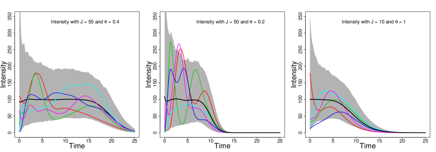
Figure 2: Prior mean (black line), prior $95\%$ interval bands (shaded area), and five individual prior realizations for the intensity under the Erlang mixture model in (1) with $(\theta,J)=$ $(0.4,50)$ (left panel), $(\theta,J)=$ $(0.2,50)$ (middle panel), and $(\theta,J)=$ $(1,10)$ (right panel). In all cases, the gamma process prior is specified with $c_{0}=0.01$ and $H_{0}(t)=t/0.01$.

2.2 Prior specification

To complete the full Bayesian model, we place prior distributions on the parameters $c_{0}$ and $b$ of the gamma process prior for $H$, and on the scale parameter $\theta$ of the Erlang basis densities. A generic approach to specify these hyperpriors can be obtained using the observation time window $(0,T)$ as the effective support of the NHPP intensity.

We work with exponential prior distributions for parameters $c_{0}$ and $b$. Using the prior mean for the intensity function, which as discussed in Section 2.1 is roughly constant at $b^{-1}$ within the time interval of interest, the total intensity in $(0,T)$ can be approximated by $T/b$. Therefore, taking the size $n$ of the observed point pattern, as a proxy for the total intensity in $(0,T)$, we can use $T/n$ to specify the mean of the exponential prior distribution for $b$. Given its role in the gamma process prior, we anticipate that small values of $c_{0}$ will be important to allow prior variability around $H_{0}$, as well as sparsity in the mixture weights. Experience from prior simulations, such as the ones shown in Figure 1, is useful to guide the range of “small” values. Note that the pattern observed in Figure 1 is not affected by the length of the observation window. In general, a value around $10$ can be viewed as a conservative guess at a high percentile for $c_{0}$. For the data examples of Section 3, we assigned an exponential prior with mean $10$ to $c_{0}$, observing substantial learning for this key model hyperparameter with its posterior distribution supported by values (much) smaller than $1$.

Also given the key role of parameter $\theta$ in controlling the intensity shapes, we recommend favoring sufficiently small values in the prior for $\theta$, especially if prior information suggests a non-standard intensity shape. Recall that $\theta$, along with $J$, control the effective support of the intensity, and thus “small” values for $\theta$ should be assessed relative to the length of the observation window. Again, prior simulation, as in Figure 2, is a useful tool. A practical approach to specify the prior range of $\theta$ values involves reducing the Erlang mixture model to the first component. The corresponding (exponential) density has mean $\theta$, and we thus use $(0,T)$ as the effective prior range for $\theta$. Because $T$ is a fairly large upper bound, and since we wish to favor smaller $\theta$ values, rather than an exponential prior, we use a Lomax prior, $p(\theta)\propto$ $(1+d_{\theta}^{-1}\theta)^{-3}$, with shape parameter equal to $2$ (thus implying infinite variance), and median $d_{\theta}(\sqrt{2}-1)$. The value of the scale parameter, $d_{\theta}$, is specified such that $\text{Pr}(0<\theta<T)\approx 0.999$. This simple strategy is effective in practice in identifying a plausible range of $\theta$ values. For the synthetic data examples of Section 3, for which $T=20$, we assigned a Lomax prior with scale parameter $d_{\theta}=1$ to $\theta$, obtaining overall moderate prior-to-posterior learning for $\theta$.

Finally, we work with fixed $J$, the value of which can be specified exploiting the role of $\theta$ and $J$ in controlling the support of the NHPP intensity. In particular, $J$ can be set equal to the integer part of $T/\theta^{*}$, where $\theta^{*}$ is the prior median for $\theta$. More conservatively, this value can be used as a lower bound for values of $J$ to be studied in a sensitivity analysis, especially for applications where one expects non-standard shapes for the intensity function. In practice, we recommend conducting prior sensitivity analysis for all model parameters, as well as plotting prior realizations and prior uncertainty bands for the intensity function to graphically explore the implications of different prior choices.

The number of Erlang basis densities is the only model parameter which is not assigned a hyperprior. Placing a prior on $J$ complicates significantly the posterior simulation method, as it necessitates use of variable-dimension MCMC techniques, while offering relatively little from a practical point of view. The key observation is again that the Erlang densities play the role of basis functions rather than of kernel densities in traditional (less structured) finite mixture models. Also key is the nonparametric nature of the prior for function $H$ that defines the mixture weights which select the Erlang densities to be used in the representation of the intensity. This model feature effectively guards against over-fitting if one conservatively chooses a larger value for $J$ than may be necessary. In this respect, the flexibility afforded by random parameters $c_{0}$ and $\theta$ is particularly useful. Overall, we have found that fixing $J$ strikes a good balance between computational tractability and model flexibility in terms of the resulting inferences.

2.3 Posterior simulation

Denote as before by $\{0<t_{1}<...<t_{n}<T\}$ the point pattern observed in time window $(0,T)$. Under the Erlang mixture model of Section 2.1, the NHPP likelihood is proportional to

$$\exp\left(-\int_{0}^{T}\lambda(u)\,\text{d}u\right)\prod_{i=1}^{n}\lambda(t_{i}) = \exp\left(-\sum\nolimits_{j=1}^{J}\omega_{j}K_{j,\theta}(T)\right)\prod_{i=1}^{n}\left\{\sum\limits_{j=1}^{J}\omega_{j}\,\text{ga}(t_{i}\mid j,\theta^{-1})\right\}$$

$$= \prod_{j=1}^{J}\exp(-\omega_{j}K_{j,\theta}(T))\prod_{i=1}^{n}\left\{\left(\sum\nolimits_{r=1}^{J}\omega_{r}\right)\sum\limits_{j=1}^{J}\left(\frac{\omega_{j}}{\sum\nolimits_{r=1}^{J}\omega_{r}}\right)\,\text{ga}(t_{i}\mid j,\theta^{-1})\right\},$$

where $K_{j,\theta}(T)=$ $\int_{0}^{T}\text{ga}(u\mid j,\theta^{-1})\,\text{d}u$ is the $j$-th Erlang distribution function at $T$.

For the posterior simulation approach, we augment the likelihood with auxiliary variables $\bm{\gamma}=$ $\{\gamma_{i}:i=1,\ldots,n\}$, where $\gamma_{i}$ identifies the Erlang basis density to which time event $t_{i}$ is assigned. Then, the augmented, hierarchical model for the data can be expressed as follows:

$$\{t_{1},...,t_{n}\}\mid\bm{\gamma},\bm{\omega},\theta \sim \prod_{j=1}^{J}\exp(-\omega_{j}K_{j,\theta}(T))\prod_{i=1}^{n}\left\{\left(\sum\nolimits_{r=1}^{J}\omega_{r}\right)\text{ga}(t_{i}\mid\gamma_{i},\theta^{-1})\right\}$$

$$\gamma_{i}\mid\bm{\omega} \stackrel{{\scriptstyle i.i.d.}}{{\sim}} \sum_{j=1}^{J}\left(\frac{\omega_{j}}{\sum\nolimits_{r=1}^{J}\omega_{r}}\right)\delta_{j}(\gamma_{i}),\quad i=1,...,n$$

$$\theta,c_{0},b,\bm{\omega} \sim p(\theta)\,p(c_{0})\,p(b)\,\prod_{j=1}^{J}\text{ga}(\omega_{j}\mid c_{0}\,\omega_{0j}(\theta),c_{0}),$$ (3)

where $\bm{\omega}=$ $\{\omega_{j}:j=1,...,J\}$, and $p(\theta)$, $p(c_{0})$, and $p(b)$ denote the priors for $\theta$, $c_{0}$, and $b$. Recall that, under the exponential distribution form for $H_{0}=t/b$, we have $\omega_{0j}(\theta)=$ $\theta/b$.

We utilize Gibbs sampling to explore the posterior distribution. The sampler involves ready updates for the auxiliary variables $\gamma_{i}$, and, importantly, also for the mixture weights $\omega_{j}$. More specifically, the posterior full conditional for each $\gamma_{i}$ is a discrete distribution on $\{1,...,J\}$ such that $\text{Pr}(\gamma_{i}=j\mid\theta,\bm{\omega},\text{data})\propto$ $\omega_{j}\,\text{ga}(t_{i}\mid j,\theta^{-1})$, for $j=1,...,J$.

Denote by $N_{j}=$ $|\{t_{i}:\gamma_{i}=j\}|$, for $j=1,...,J$, that is, $N_{j}$ is the number of time points assigned to the $j$-th Erlang basis density. The posterior full conditional distribution for $\omega$ is derived as follows:

$$p(\bm{\omega}\mid\theta,c_{0},b,\bm{\gamma},\text{data}) \propto \left\{\prod_{j=1}^{J}\exp(-\omega_{j}K_{j,\theta}(T))\right\}\left(\sum\nolimits_{r=1}^{J}\omega_{r}\right)^{n}$$

$$\times \left\{\prod_{j=1}^{J}\omega_{j}^{N_{j}}\left(\sum\nolimits_{r=1}^{J}\omega_{r}\right)^{-N_{j}}\right\}\left\{\prod_{j=1}^{J}\text{ga}(\omega_{j}\mid c_{0}\,\omega_{0j}(\theta),c_{0})\right\}$$

$$\propto \prod_{j=1}^{J}\exp(-\omega_{j}K_{j,\theta}(T))\,\omega_{j}^{N_{j}}\,\text{ga}(\omega_{j}\mid c_{0}\,\omega_{0j}(\theta),c_{0})$$

$$= \prod_{j=1}^{J}\text{ga}(\omega_{j}\mid N_{j}+c_{0}\,\omega_{0j}(\theta),K_{j,\theta}(T)+c_{0}),$$

where we have used the fact that $\sum_{j=1}^{J}N_{j}=n$. Therefore, given the other parameters and the data, the mixture weights are independent, and each $\omega_{j}$ follows a gamma posterior full conditional distribution. This is a practically important feature of the model in terms of convenient updates for the mixture weights, and with respect to efficiency of the posterior simulation algorithm as it pertains to this key component of the model parameter vector.

Finally, each of the remaining parameters, $c_{0}$, $b$, and $\theta$, is updated with a Metropolis-Hastings (M-H) step, using a log-normal proposal distribution in each case.

2.4 Model extensions to incorporate marks

Here, we discuss how the Erlang mixture prior for NHPP intensities can be embedded in semiparametric models for point patterns that include additional information on marks.

Consider the setting where, associated with each observed time event $t_{i}$, marks $\bm{y}_{i}\equiv$ $\bm{y}_{t_{i}}$ are recorded (marks are only observed when an event is observed). Without loss of generality, we assume that marks are continuous variables taking values in mark space ${\cal M}\subseteq\mathbb{R}^{d}$, for $d\geq 1$. As discussed in Taddy and Kottas, (2012), a nonparametric prior for the intensity of the temporal process, ${\cal T}$, can be combined with a mark distribution to construct a semiparametric model for marked NHPPs. In particular, consider a generic marked NHPP $\{(t,\bm{y}_{t}):t\in{\cal T},\bm{y}_{t}\in{\cal M}\}$, that is: the temporal process ${\cal T}$ is a NHPP on $\mathbb{R}^{+}$ with intensity function $\lambda$; and, conditional on ${\cal T}$, the marks $\{\bm{y}_{t}:t\in{\cal T}\}$ are mutually independent. Now, assume that, conditional on ${\cal T}$, the marks have density $m_{t}$ that depends only on $t$ (i.e., it does not depend on any earlier time $t^{\prime}<t$). Then, by the “marking” theorem (e.g., Kingman, 1993), we have that the marked NHPP is a NHPP on the extended space $\mathbb{R}^{+}\times{\cal M}$ with intensity $\lambda^{*}(t,\bm{y}_{t})=$ $\lambda(t)\,m_{t}(\bm{y}_{t})$. Therefore, the likelihood for the observed marked point pattern $\{(t_{i},\bm{y}_{i}):i=1,...,n\}$ can be written as $\exp\left(-\int_{0}^{T}\lambda(u)\,\text{d}u\right)\prod_{i=1}^{n}\lambda(t_{i})\prod_{i=1}^{n}m_{t_{i}}(\bm{y}_{i})$ (the integral $\int_{0}^{T}\int_{{\cal M}}\lambda^{*}(u,\bm{z})\,\text{d}u\text{d}\bm{z}$ in the normalizing term reduces to $\int_{0}^{T}\lambda(u)\,\text{d}u$, since $m_{t}$ is a density). Hence, the MCMC method of Section 2.3 can be extended for marked NHPP models built from the Erlang mixture prior for intensity $\lambda$, and any time-dependent model for the mark density $m_{t}$.

3 Data examples

To empirically investigate inference under the proposed model, we present three synthetic data examples corresponding to decreasing, increasing, and bimodal intensities. We also consider the coal-mining disasters data set, which is commonly used to illustrate NHPP intensity estimation.

We used the approach of Section 2.2 to specify the priors for $c_{0}$, $b$ and $\theta$, and the value for $J$. In particular, we used the exponential prior for $c_{0}$ with mean $10$ for all data examples. For the three synthetic data sets (for which $T=20$), we used the Lomax prior for $\theta$ with shape parameter equal to $2$ and scale parameter equal to $1$. Prior sensitivity analysis results for the synthetic data example of Section 3.3 are provided in the Supplementary Material. Overall, results from prior sensitivity analysis (also conducted for all other data examples) suggest that the prior specification approach of Section 2.2 is effective as a general strategy. Moreover, more dispersed priors for parameters $c_{0}$, $b$ and $\theta$ have little to no effect on the posterior distribution for these parameters and essentially no effect on posterior estimates for the NHPP intensity function, even for point patterns with relatively small size, such as the one ($n=112$) for the data example of Section 3.3.

The Supplement provides also computational details about the MCMC posterior simulation algorithm, including study of the effect of the number of basis densities ($J$) and the size of the point pattern ($n$) on effective sample size and computing time.

3.1 Decreasing intensity synthetic point pattern

The first synthetic data set involves $491$ time points generated in time window $(0,20)$ from a NHPP with intensity function $\beta^{-1}\alpha(\beta^{-1}t)^{\alpha-1}$, where $(\alpha,\beta)=$ $(0.5,8\times 10^{-5})$. This form corresponds to the hazard function of a Weibull distribution with shape parameter less than $1$, thus resulting in a decreasing intensity function.

The Erlang mixture model was applied with $J=50$, and an exponential prior for $b$ with mean $0.04$. The model captures the decreasing pattern of the data generating intensity function; see Figure 3. We note that there is significant prior-to-posterior learning in the intensity function estimation; the prior intensity mean is roughly constant at value about $25$ with prior uncertainty bands that cover almost the entire top left panel in Figure 3. Prior uncertainty bands were similarly wide for all other data examples.

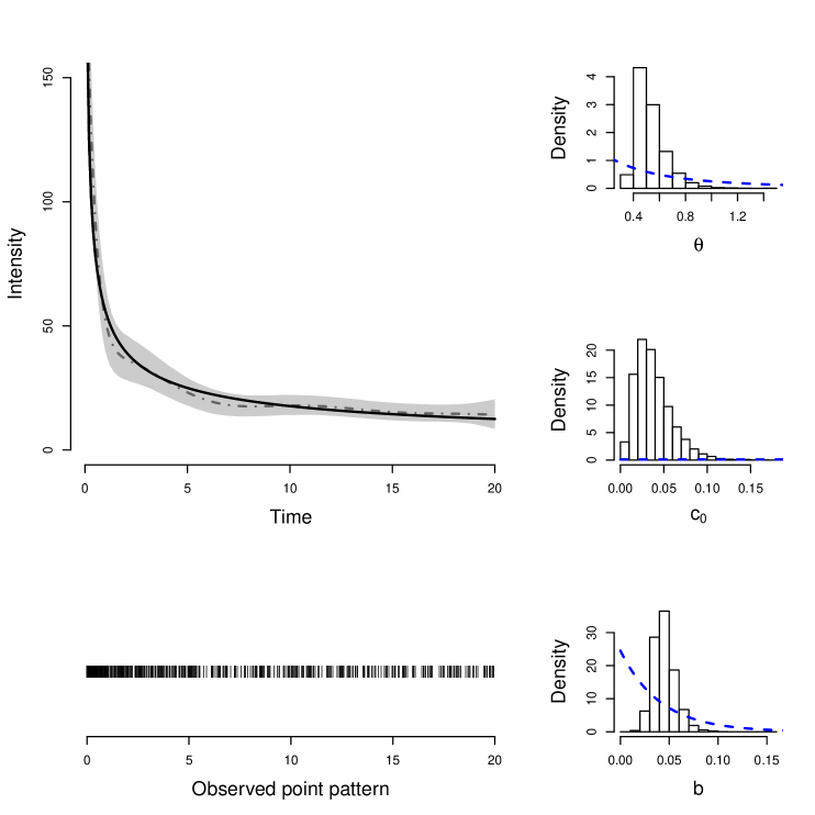
Figure 3: Synthetic data from temporal NHPP with decreasing intensity. The top left panel shows the posterior mean estimate (dashed-dotted line) and posterior 95% interval bands (shaded area) for the intensity function. The true intensity is denoted by the solid line. The point pattern is plotted in the bottom left panel. The three plots on the right panels display histograms of the posterior samples for the model hyperparameters, along with the corresponding prior densities (dashed lines).

3.2 Increasing intensity synthetic point pattern

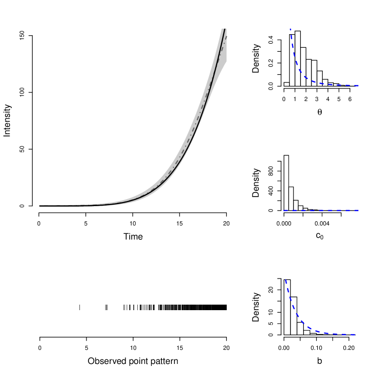
Figure 4: Synthetic data from temporal NHPP with increasing intensity. The top left panel shows the posterior mean estimate (dashed-dotted line) and posterior 95% interval bands (shaded area) for the intensity function. The true intensity is denoted by the solid line. The point pattern is plotted in the bottom left panel. The three plots on the right panels display histograms of the posterior samples for the model hyperparameters, along with the corresponding prior densities (dashed lines).

We consider again the form $\beta^{-1}\alpha(\beta^{-1}t)^{\alpha-1}$ for the NHPP intensity function, but here with $(\alpha,\beta)=$ $(6,7)$ such that the intensity is increasing. A point pattern comprising $565$ points was generated in time window $(0,20)$. The Erlang mixture model was applied with $J=50$, and an exponential prior for $b$ with mean $0.035$. Figure 4 reports inference results. This example demonstrates the model’s capacity to effectively recover increasing intensity shapes over the bounded observation window, even though the Erlang basis densities are ultimately decreasing.

3.3 Bimodal intensity synthetic point pattern

The data examples in Sections 3.1 and 3.2 illustrate the model’s capacity to uncover monotonic intensity shapes, associated with a parametric distribution different from the Erlang distribution that forms the basis of the mixture intensity model. Here, we consider a point pattern generated from a NHPP with a more complex intensity function, $\lambda(t)=$ $50\,\text{We}(t\mid 3.5,5)$ + $60\,\text{We}(t\mid 6.5,15)$, where $\text{We}(t\mid\alpha,\beta)$ denotes the Weibull density with shape parameter $\alpha$ and mean $\beta\,\Gamma(1+1/\alpha)$. This specification results in a bimodal intensity within the observation window $(0,20)$ where a synthetic point pattern of $112$ time points is generated; see Figure 5.

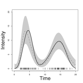
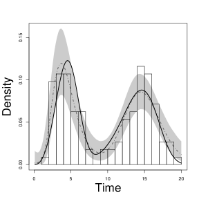
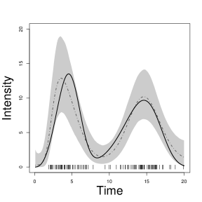
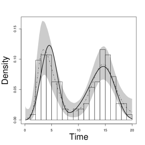
Figure 5: Synthetic data from temporal NHPP with bimodal intensity. Inference results are reported under $J=50$ (top row) and $J=100$ (bottom row). The left column plots the posterior means (circles) and 90% interval estimates (bars) of the weights for the Erlang basis densities. The middle column displays the posterior mean estimate (dashed-dotted line) and posterior 95% interval bands (shaded area) for the NHPP intensity function. The true intensity is denoted by the solid line. The bars on the horizontal axis indicate the point pattern. The right column plots the posterior mean estimate (dashed-dotted line) and posterior 95% interval bands (shaded area) for the NHPP density function on the observation window. The histogram corresponds to the simulated times that comprise the point pattern.

We used an exponential prior for $b$ with mean $0.179$. Anticipating an underlying intensity with less standard shape than in the earlier examples, we compare inference results under $J=50$ and $J=100$; see Figure 5. The posterior point and interval estimates capture effectively the bimodal intensity shape, especially if one takes into account the relatively small size of the point pattern. (In particular, the histogram of the simulated random time points indicates that they do not provide an entirely accurate depiction of the underlying NHPP density shape.) The estimates are somewhat more accurate under $J=100$. The estimates for the mixture weights (left column of Figure 5) indicate the subsets of the Erlang basis densities that are utilized under the two different values for $J$. The posterior mean of $\theta$ was $0.366$ under $J=50$, and $0.258$ under $J=100$, that is, as expected, inference for $\theta$ adjusts to different values of $J$ such that $(0,J\theta)$ provides roughly the effective support of the intensity.

3.4 Coal-mining disasters data

Our real data example involves the “coal-mining disasters” data (e.g., Andrews and Herzberg, 1985, p. 53-56), a standard dataset used in the literature to test NHPP intenstiy estimation methods. The point pattern comprises the times (in days) of $n=191$ explosions of fire-damp or coal-dust in mines resulting in 10 or more casualties from the accident. The observation window consists of 40,550 days, from March 15, 1851 to March 22, 1962.

We fit the Erlang mixture model with $J=50$, using a Lomax prior for $\theta$ with shape parameter $2$ and scale parameter $2,000$, such that $\text{Pr}(0<\theta<40,550)\approx 0.998$, and an exponential prior for $b$ with mean $213$. We also implemented the model with $J=130$, obtaining essentially the same inference results for the NHPP functionals with the ones reported in Figure 6.

The estimates for the point process intensity and density functions (Figure 6, top row) suggest that the model successfully captures the multimodal intensity shape suggested by the data. The estimates for the mixture weights (Figure 6, bottom left panel) indicate the Erlang basis densities that are more influential to the model fit.

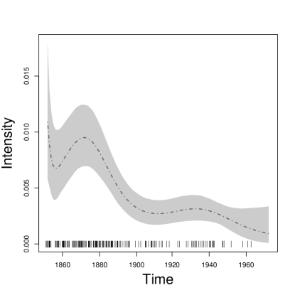
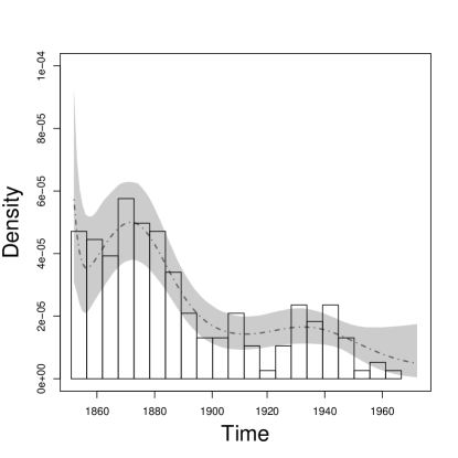
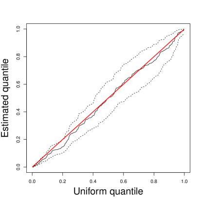
Figure 6: Coal-mining disasters data. The top left panel shows the posterior mean estimate (dashed-dotted line) and 95% interval bands (shaded area) for the intensity function. The bars at the bottom indicate the observed point pattern. The top right panel plots the posterior mean (dashed-dotted line) and 95% interval bands (shaded area) for the NHPP density, overlaid on the histogram of the accident times. The bottom left panel presents the posterior means (circles) and 90% interval estimates (bars) of the mixture weights. The bottom right panel plots the posterior mean and 95% interval bands for the time-rescaling model checking Q-Q plot.

The bottom right panel of Figure 6 reports results from graphical model checking, using the “time-rescaling” theorem (e.g., Daley and Vere-Jones, 2003). If the point pattern $\{0=t_{0}<t_{1}<...<t_{n}<T\}$ is a realization from a NHPP with cumulative intensity function $\Lambda(t)=$ $\int_{0}^{t}\lambda(u)\text{d}u$, then the transformed point pattern $\{\Lambda(t_{i}):i=1,...,n\}$ is a realization from a unit rate homogeneous Poisson process. Therefore, if we further transform to $U_{i}=$ $1-\exp\{-(\Lambda(t_{i})-\Lambda(t_{i-1}))\}$, where $\Lambda(0)\equiv 0$, then the $\{U_{i}:i=1,...,n\}$ are independent uniform$(0,1)$ random variables. Hence, graphical model checking can be based on quantile–quantile (Q-Q) plots to assess agreement of the estimated $U_{i}$ with the uniform distribution on the unit interval. Under the Bayesian inference framework, we can obtain a posterior sample for the $U_{i}$ for each posterior realization for the NHPP intensity, and we can thus plot posterior point and interval estimates for the Q-Q graph. These estimates suggest that the NHPP model with the Erlang mixture intensity provides a good fit for the coal-mining disasters data.

4 Modeling for spatial Poisson process intensities

In Section 4.1, we extend the modeling framework to spatial NHPPs with intensities defined on $\mathbb{R}^{+}\times\mathbb{R}^{+}$. The resulting inference method is illustrated with synthetic and real data examples in Section 4.2 and 4.3, respectively.

4.1 The Erlang mixture model for spatial NHPPs

A spatial NHPP is again characterized by its intensity function, $\lambda(\bm{s})$, for $\bm{s}=(s_{1},s_{2})\in\mathbb{R}^{+}\times\mathbb{R}^{+}$. The NHPP intensity is a non-negative and locally integrable function such that: (a) for any bounded $B\subset\mathbb{R}^{+}\times\mathbb{R}^{+}$, the number of points in $B$, $N(B)$, follows a Poisson distribution with mean $\int_{B}\lambda(\bm{u})\,\text{d}\bm{u}$; and (b) given $N(B)=n$, the random locations $\bm{s}_{i}=$ $(s_{i1},s_{i2})$, for $i=1,...,n$, that form the spatial point pattern in $B$ are i.i.d. with density $\lambda(\bm{s})/\{\int_{B}\lambda(\bm{u})\,\text{d}\bm{u}\}$. Therefore, the structure of the likelihood for the intensity function is similar to the temporal NHPP case. In particular, for spatial point pattern, $\{\bm{s}_{1},\ldots,\bm{s}_{n}\}$, observed in bounded region $D\subset\mathbb{R}^{+}\times\mathbb{R}^{+}$, the likelihood is proportional to $\exp\{-\int_{D}\lambda(\bm{u})\,\text{d}\bm{u}\}\,\prod_{i=1}^{n}\lambda(\bm{s}_{i})$. As is typically the case in standard applications involving spatial NHPPs, we consider a regular, rectangular domain for the observation region $D$, which can therefore be taken without loss of generality to be the unit square.

Extending the Erlang mixture model in (1), we build the basis representation for the spatial NHPP intensity from products of Erlang densities, $\{\text{ga}(s_{1}\mid j_{1},\theta^{-1}_{1})\,\text{ga}(s_{2}\mid j_{2},\theta^{-1}_{2}):j_{1},j_{2}=1,...,J\}$. Mixing is again with respect to the shape parameters $(j_{1},j_{2})$, and the basis densities share a pair of scale parameters $(\theta_{1},\theta_{2})$. Therefore, the model can be expressed as

$$\lambda(s_{1},s_{2})=\sum^{J}_{j_{1}=1}\sum^{J}_{j_{2}=1}\omega_{j_{1}j_{2}}\,\text{ga}(s_{1}\mid j_{1},\theta^{-1}_{1})\,\text{ga}(s_{2}\mid j_{2},\theta^{-1}_{2}),\,\,\,\,\,\,\,(s_{1},s_{2})\in\mathbb{R}^{+}\times\mathbb{R}^{+}.$$

Again, a key model feature is the prior for the mixture weights. Here, the basis density indexed by $(j_{1},j_{2})$ is associated with rectangle $A_{j_{1}j_{2}}=$ $[(j_{1}-1)\theta_{1},j_{1}\theta_{1})\times[(j_{2}-1)\theta_{2},j_{2}\theta_{2})$. The corresponding weight is defined through a random measure $H$ supported on $\mathbb{R}^{+}\times\mathbb{R}^{+}$, such that $\omega_{j_{1}j_{2}}=$ $H(A_{j_{1}j_{2}})$. This construction extends the one for the weights of the temporal NHPP model. We again place a gamma process prior, $\mathcal{G}(H_{0},c_{0})$, on $H$, where $c_{0}$ is the precision parameter and $H_{0}$ is the centering measure on $\mathbb{R}^{+}\times\mathbb{R}^{+}$. As a natural extension of the exponential cumulative hazard used in Section 2.1 for the gamma process prior mean, we specify $H_{0}$ to be proportional to area. In particular, $H_{0}(A_{j_{1}j_{2}})=$ $|A_{j_{1}j_{2}}|/b=$ $\theta_{1}\theta_{2}/b$, where $b>0$. Using the independent increments property of the gamma process, and under the specific choice of $H_{0}$, the prior for the mixture weights is given by

$$\omega_{j_{1}j_{2}}\mid\theta_{1},\theta_{2},c_{0},b\,\stackrel{{\scriptstyle i.i.d.}}{{\sim}}\,\text{ga}(\omega_{j_{1}j_{2}}\mid c_{0}\,\theta_{1}\,\theta_{2}\,b^{-1},c_{0}),\,\,\,\,\,\,\,j_{1},j_{2}=1,...,J,$$

which, as before, is a practically important feature of the model construction as it pertains to MCMC posterior simulation.

To complete the full Bayesian model, we place priors on the common scale parameters for the basis densities, $(\theta_{1},\theta_{2})$, and on the gamma process prior hyperparameters $c_{0}$ and $b$. The role played by these model parameters is directly analogous to the one of the corresponding parameters for the temporal NHPP model, as detailed in Section 2.1. Therefore, we apply similar arguments to the ones in Section 2.2 to specify the model hyperpriors. More specifically, we work with (independent) Lomax prior distributions for scale parameters $\theta_{1}$ and $\theta_{2}$, where the shape parameter of the Lomax prior is set equal to $2$ and the scale parameter is specified such that $\text{Pr}(0<\theta_{1}<1)\text{Pr}(0<\theta_{2}<1)\approx 0.999$. Recall that the observation region is taken to be the unit square; in general, for a square observation region, this approach implies the same Lomax prior for $\theta_{1}$ and $\theta_{2}$. The gamma process precision parameter $c_{0}$ is assigned an exponential prior with mean $10$. The result of Section 2.1 for the prior mean of the NHPP intensity can be extended to show that $\text{E}(\lambda(s_{1},s_{2})\mid b,\theta_{1},\theta_{2})$ converges to $b^{-1}$, as $J\rightarrow\infty$, for any $(s_{1},s_{2})\in\mathbb{R}^{+}\times\mathbb{R}^{+}$, and for any $(\theta_{1},\theta_{2})$ (and $c_{0}$). The prior mean for the spatial NHPP intensity is practically constant at $b^{-1}$ within its effective support given roughly by $(0,J\theta_{1})\times(0,J\theta_{2})$. Hence, taking the size of the observed spatial point pattern as a proxy for the total intensity, $b$ is assigned an exponential prior distribution with mean $1/n$. Finally, the choice of the value for $J$ can be guided from the approximate effective support for the intensity, which is controlled by $J$ along with $\theta_{1}$ and $\theta_{2}$. Analogously to the approach discussed in Section 2.2, the value of $J$ (or perhaps a lower bound for $J$) can be specified through the integer part of $1/\theta^{\ast}$, where $\theta^{\ast}$ is the median of the common Lomax prior for $\theta_{1}$ and $\theta_{2}$.

The posterior simulation method for the spatial NHPP model is developed through a straightforward extension of the approach detailed in Section 2.3. We work again with the augmented model that involves latent variables $\{\bm{\gamma}_{i}:i=1,\ldots,n\}$, where $\bm{\gamma}_{i}=$ $(\gamma_{i1},\gamma_{i2})$ identifies the basis density to which observed point location $(s_{i1},s_{i2})$ is assigned. The spatial NHPP model retains the practically relevant feature of efficient updates for the mixture weights, which, given the other model parameters and the data, have independent gamma posterior full conditional distributions. Details of the MCMC posterior simulation algorithm are provided in the Supplementary Material.

4.2 Synthetic data example

Here, we illustrate the spatial NHPP model using synthetic data based on a bimodal intensity function built from a two-component mixture of bivariate logit-normal densities. Denote by $\text{BLN}(\bm{\mu},\Sigma)$ the bivariate logit-normal density arising from the logistic transformation of a bivariate normal with mean vector $\bm{\mu}$ and covariance matrix $\Sigma$. A spatial point pattern of size $528$ was generated over the unit square from a NHPP with intensity $\lambda(s_{1},s_{2})=$ $150\,\text{BLN}((s_{1},s_{2})\mid\bm{\mu}_{1},\Sigma)\,+\,350\,\text{BLN}((s_{1},s_{2})\mid\bm{\mu}_{2},\Sigma)$, where $\bm{\mu}_{1}=$ $(-1,1)$, $\bm{\mu}_{2}=$ $(1,-1)$, and $\Sigma=$ $(\sigma_{11},\sigma_{12},\sigma_{21},\sigma_{22})=$ $(0.3,0.1,0.1,0.3)$. The intensity function and the generated spatial point pattern are shown in the top left panel of Figure 7.

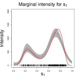
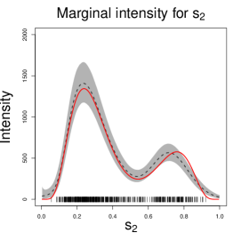
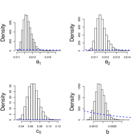
Figure 7: Synthetic data example from spatial NHPP. The top row panels show contour plots of the true intensity, and of the posterior mean and interquartile range estimates. The points in each panel indicate the observed point pattern. The first two panels at the bottom row show the marginal intensity estimates – posterior mean (dashed line) and 95% uncertainty bands (shaded area) – along with the true function (red solid line) and corresponding point pattern (bars at the bottom of each panel). The bottom right panel displays histograms of posterior samples for the model hyperparameters along with the corresponding prior densities (dashed lines).

The Erlang mixture model was applied setting $J=70$ and using the hyperpriors for $\theta_{1}$, $\theta_{2}$, $c_{0}$ and $b$ discussed in Section 4.1. Figure 7 reports inference results. The posterior mean intensity estimate successfully captures the shape of the underlying intensity function. The structure of the Erlang mixture model enables ready inference for the marginal NHPP intensities associated with the two-dimensional NHPP. Although such inference is generally not of direct interest for spatial NHPPs, in the context of a synthetic data example it provides an additional means to check the model fit. The marginal intensity estimates effectively retrieve the bimodality of the true marginal intensity functions; the slight discrepancy at the second mode can be explained by inspection of the generated data for which the second mode clusters are located slightly to the left of the theoretical mode. Finally, we note the substantial prior-to-posterior learning for all model hyperparameters.

4.3 Real data illustration

Our final data example involves a spatial point pattern that has been previously used to illustrate NHPP intensity estimation methods (e.g., Diggle,, 2014; Kottas and Sansó,, 2007). The data set involves the locations of 514 maple trees in a 19.6 acre square plot in Lansing Woods, Clinton County, Michigan, USA; the maple trees point pattern is included in the left column panels of Figure 8.

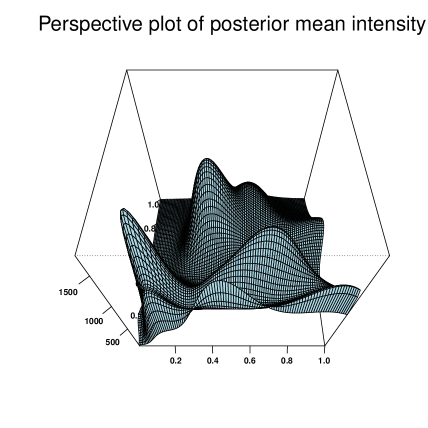
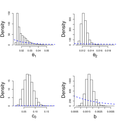
Figure 8: Maple trees data. The top row panels show the posterior mean estimate for the intensity function in the form of contour and perspective plots. The bottom left panel displays the corresponding posterior interquartile range contour plot. The bottom right panel plots histograms of posterior samples for the model hyperparameters along with the corresponding prior densities (dashed lines). The points in the left column plots indicate the locations of the 514 maple trees.

To apply the spatial Erlang mixture model, we specified the hyperpriors for $\theta_{1}$, $\theta_{2}$, $c_{0}$ and $b$ following the approach discussed in Section 4.1, and set $J=70$. As with the synthetic data example, the posterior distributions for model hyperparameters are substantially concentrated relative to their priors; see the bottom right panel of Figure 8. The estimates for the spatial intensity of maple tree locations reported in Figure 8 demonstrate the model’s capacity to uncover non-standard, multimodal intensity surfaces.

5 Discussion

We have proposed a Bayesian nonparametric modeling approach for Poisson processes over time or space. The approach is based on a mixture representation of the point process intensity through Erlang basis densities, which are fully specified save for a scale parameter shared by all of them. The weights assigned to the Erlang densities are defined through increments of a random measure (a random cumulative intensity function in the temporal NHPP case) which is modeled with a gamma process prior. A key feature of the methodology is that it offers a good balance between model flexibility and computational efficiency in implementation of posterior inference. Such inference has been illustrated with synthetic and real data for both temporal and spatial Poisson process intensities.

To discuss our contribution in the context of Bayesian nonparametric modeling methods for NHPPs (briefly reviewed in the Introduction), note that the main approaches can be grouped into two broad categories: placing the prior model on the NHPP intensity function; or, assigning separate priors to the total intensity and the NHPP density (both defined over the observation window).

In terms of applications, especially for spatial point patterns, the most commonly explored class of models falling in the former category involves Gaussian process (GP) priors for logarithmic (or logit) transformations of the NHPP intensity (e.g., Møller et al.,, 1998; Adams et al.,, 2009). The NHPP likelihood normalizing term renders full posterior inference under GP-based models particularly challenging. This challenge has been bypassed using approximations of the stochastic integral that defines the likelihood normalizing term (Brix and Diggle, 2001, Brix and Møller, 2001), data augmentation techniques (Adams et al.,, 2009), and different types of approximations of the NHPP likelihood along with integrated nested Laplace approximation for approximate Bayesian inference (Illian et al., 2012, Simpson et al., 2016). In contrast, the Erlang mixture model can be readily implemented with MCMC algorithms that do not involve approximations to the NHPP likelihood or complex computational techniques. The Supplementary Material includes comparison of the proposed model with two GP-based models: the sigmoidal Gaussian Cox process (SGCP) model (Adams et al.,, 2009) for temporal NHPPs; and the log-Gaussian Cox process (LGCP) model for spatial NHPPs, as implemented in the R package lgcp (Taylor et al.,, 2013). The results, based on the synthetic data considered in Sections 3.3 and 4.2, suggest that the Erlang mixture model is substantially more computationally efficient than the SGCP model, as well as less sensitive to model/prior specification than LGCP models for which the choice of the GP covariance function can have a large effect on the intensity surface estimates.

Since it involves a mixture formulation for the NHPP intensity, the proposed modeling approach is closer in spirit to methods based on Dirichlet process mixture priors for the NHPP density (e.g., Kottas and Sansó,, 2007; Taddy and Kottas,, 2012). Both types of approaches build posterior simulation from standard MCMC techniques for mixture models, using latent variables that configure the observed points to the mixture components. Models that build from density estimation with Dirichlet process mixtures benefit from the wide availability of related posterior simulation methods (e.g., the number of mixture components in the NHPP density representation does not need to be specified), and from the various extensions of the Dirichlet process for dependent distributions that can be explored to develop flexible models for hierarchically related point processes (e.g., Taddy,, 2010; Kottas et al.,, 2012; Xiao et al.,, 2015; Rodriguez et al.,, 2017). However, by construction, this approach is restricted to modeling the NHPP intensity only on the observation window, in fact, with a separate prior for the NHPP density and for the total intensity over the observation window. The Erlang mixture model overcomes this limitation. For instance, in the temporal case, the prior model supports the intensity on $\mathbb{R}^{+}$, and the priors for the total intensity and the NHPP density over $(0,T)$ (given in Equation (2)) are compatible with the prior for the NHPP intensity.

The proposed model admits a parsimonious representation for the NHPP intensity with the Erlang basis densities defined through a single parameter, the common scale parameter $\theta$. Such intensity representations offer a nonparametric Bayesian modeling perspective for point processes that may be attractive in other contexts and for different types of applications. For instance, Zhao and Kottas, (2021) study representations for the intensity through weighted combinations of structured beta densities (with different priors for the mixture weights), which are particularly well suited to flexible and efficient inference for spatial NHPP intensities over irregular domains.

Finally, we note that the Erlang mixture prior model is useful as a building block towards Bayesian nonparametric inference for point processes that can be represented as hierarchically structured, clustered NHPPs. Current research is exploring fully nonparametric modeling for a key example, the Hawkes process (Hawkes, 1971), using the Erlang mixture prior for the Hawkes process immigrant (background) intensity function.

Supplementary Information

The Supplementary Material includes results from prior sensitivity analysis, information on computing times and effective sample sizes, the technical details of the MCMC algorithm for the spatial NHPP model, and results from comparison of the Erlang mixture model with two Gaussian process based models for temporal or spatial NHPPs.

References

- Adams et al., (2009) Adams, R. P., Murray, I., and MacKay, D. J. C. (2009). Tractable nonparametric Bayesian inference in Poisson processes with Gaussian process intensities. In Proceedings of the 26th International Conference on Machine Learning, Montreal, Canada.
- Andrews and Herzberg, (1985) Andrews, D. F. and Herzberg, A. M. (1985). Data, A Collection of Problems from Many Fields for the Student and Research Worker. Springer-Verlag.
- Brix and Diggle, (2001) Brix, A. and Diggle, P. J. (2001). Spatiotemporal prediction for log-Gaussian Cox processes. Journal of the Royal Statistical Society. Series B, 63:823–841.
- Brix and Møller, (2001) Brix, A. and Møller, J. (2001). Space-time multi type log Gaussian Cox processes with a view to modelling weeds. Scandinavian Journal of Statistics, 28:471–488.
- Butzer, (1954) Butzer, P. L. (1954). On the extensions of Bernstein polynomials to the infinite interval. Proceedings of the American Mathematical Society, 5:547–553.
- Daley and Vere-Jones, (2003) Daley, D. J. and Vere-Jones, D. (2003). An Introduction to the Theory of Point Processes(2nd edition). Springer.
- Diggle, (2014) Diggle, P. J. (2014). Statistical Analysis of Spatial and Spatio-Temporal Point Paterterns(3rd edition). CRC press.
- Ferguson, (1973) Ferguson, T. S. (1973). A Bayesian analysis of some nonparametric problems. The Annals of Statistics, 1:209–230.
- Ghosal and van der Vaart, (2017) Ghosal, S. and van der Vaart, A. (2017). Fundamentals of Nonparametric Bayesian Inference. Cambridge University Press.
- Hawkes, (1971) Hawkes, A. G. (1971). Point spectra of some mutually exciting point processes. Journal of the Royal Statistical Society. Series B, 33(3):438–443.
- Heikkinen and Arjas, (1998) Heikkinen, J. and Arjas, E. (1998). Non-parametric Bayesian estimation of a spatial Poisson intensity. Scandinavian Journal of Statistics, 25:435–450.
- Heikkinen and Arjas, (1999) Heikkinen, J. and Arjas, E. (1999). Modeling a Poisson forest in variable elevations: A nonparametric Bayesian approach. Biometrics, 55:738–745.
- Illian et al., (2012) Illian, J. B., Sørbye, S. H., and Rue, H. (2012). A toolbox for fitting complex spatial point process models using integrated nested Laplace approximation (INLA). The Annals of Applied Statistics, 6:1499–1530.
- Ishwaran and James, (2004) Ishwaran, H. and James, L. F. (2004). Computational methods for multiplicative intensity models using weighted gamma processes: Proportional hazards, marked point processes, and panel count data. Journal of the American Statistical Association, 99:175–190.
- Kalbfleisch, (1978) Kalbfleisch, J. D. (1978). Non-parametric Bayesian analysis of survival time data. Journal of the Royal Statistical Society. Series B, 40:214–221.
- Kang et al., (2014) Kang, J., Nichols, T. E., Wager, T. D., and Johnson, T. D. (2014). A Bayesian hierarchical spatial point process model for multi-type neuroimaging meta-analysis. The Annals of Applied Statistics, 8:1800–1824.
- Kingman, (1993) Kingman, J. F. C. (1993). Poisson Processes. Clarendon Press.
- Kottas, (2006) Kottas, A. (2006). Dirichlet process mixtures of Beta distributions, with applications to density and intensity estimation. In Proceedings of the Workshop on Learning with Nonparametric Bayesian Methods, 23rd International Conference on Machine Learning, Pittsburgh, PA, USA.
- Kottas et al., (2012) Kottas, A., Behseta, S., Moorman, D., Poynor, V., and Olson, C. (2012). Bayesian nonparametric analysis of neuronal intensity rates. Journal of Neuroscience Methods, 203:241–253.
- Kottas and Sansó, (2007) Kottas, A. and Sansó, B. (2007). Bayesian mixture modeling for spatial Poisson process intensities, with applications to extreme value analysis. Journal of Statistical Planning and Inference, 137:3151–3163.
- Lee and Lin, (2010) Lee, S. C. K. and Lin, X. S. (2010). Modeling and evaluating insurance losses via mixtures of Erlang distributions. North American Actuarial Journal, 14:107–130.
- Lo, (1982) Lo, A. Y. (1982). Bayesian nonparametric statistical inference for Poisson point processes. Z. Wahrscheinlichkeitstheorie verw. Gebiete, 59:55–66.
- Lo, (1992) Lo, A. Y. (1992). Bayesian inference for Poisson process models with censored data. Journal of Nonparametric Statistics, 2:71–80.
- Lo and Weng, (1989) Lo, A. Y. and Weng, C. S. (1989). On a class of Bayesian nonparametric estimates: ii. hazard rate estimates. Annals of the Institute for Statistical Mathematics, 41:227–245.
- Møller et al., (1998) Møller, J., Syversveen, A. R., and Waagepetersen, R. P. (1998). Log Gaussian Cox processes. Scandinavian Journal of Statistics, 25:451–482.
- (26) Petrone, S. (1999a). Bayesian density estimation using Bernstein polynomials. Canadian Journal of Statistics, 27:105–126.
- (27) Petrone, S. (1999b). Random Bernstein polynomials. Scandinavian Journal of Statistics, 26:373–393.
- Rodrigues and Diggle, (2012) Rodrigues, A. and Diggle, P. J. (2012). Bayesian estimation and prediction for inhomogeneous spatiotemporal log-Gaussian Cox processes using low-rank models, with application to criminal surveillance. Journal of the American Statistical Association, 107:93–101.
- Rodriguez et al., (2017) Rodriguez, A., Wang, Z., and Kottas, A. (2017). Assessing systematic risk in the S&P500 index between 2000 and 2011: A Bayesian nonparametric approach. The Annals of Applied Statistics, 11:527–552.
- Simpson et al., (2016) Simpson, D., Illian, J. B., Lindgren, F., Sørbye, S. H., and Rue, H. (2016). Going off grid: computationally efficient inference for log-Gaussian Cox processes. Biometrika, 103:49–70.
- Taddy, (2010) Taddy, M. (2010). Autoregressive mixture models for dynamic spatial Poisson processes: Application to tracking the intensity of violent crime. Journal of the American Statistical Association, 105:1403–1417.
- Taddy and Kottas, (2012) Taddy, M. A. and Kottas, A. (2012). Mixture modeling for marked Poisson processes. Bayesian Analysis, 7:335–362.
- Taylor et al., (2013) Taylor, B., Davies, T., Rowlingson, B., and Diggle, P. (2013). lgcp: An R package for inference with spatial and spatio-temporal log-Gaussian Cox processes. Journal of Statistical Software, 52:1–40.
- Venturini et al., (2008) Venturini, S., Dominici, F., and Parmigiani, G. (2008). Gamma shape mixtures for heavy-tailed distributions. The Annals of Applied Statistics, 2:756–776.
- Wolpert and Ickstadt, (1998) Wolpert, R. L. and Ickstadt, K. (1998). Poisson/gamma random field models for spatial statistics. Biometrika, 85:251–267.
- Xiao et al., (2015) Xiao, S., Kottas, A., and Sansó, B. (2015). Modeling for seasonal marked point processes: An analysis of evolving hurricane occurrences. The Annals of Applied Statistics, 9:353–382.
- Xiao et al., (2021) Xiao, S., Kottas, A., Sansó, B., and Kim, H. (2021). Nonparametric Bayesian modeling and estimation for renewal processes. Technometrics, 63:100–115.
- Zhao and Kottas, (2021) Zhao, C. and Kottas, A. (2021). Modeling for Poisson process intensities over irregular spatial domains. arXiv:2106.04654 [stat.ME].