Parallel Peeling of Bipartite Networks for Hierarchical Dense Subgraph Discovery

Abstract.

Motif-based graph decomposition is widely used to mine hierarchical dense structures in graphs. In bipartite graphs, wing and tip decomposition construct a hierarchy of butterfly (2,2-biclique) dense edge and vertex induced subgraphs, respectively. They have applications in several domains including e-commerce, recommendation systems and document analysis.

Existing decomposition algorithms use a bottom-up approach that constructs the hierarchy in an increasing order of subgraph density. They iteratively select the entities (edges or vertices) with minimum support (butterfly count) and peel them i.e. remove them from them graph and update the support of other entities. The amount of butterflies in real-world bipartite graphs makes bottom-up peeling computationally demanding. Furthermore, the strict order of peeling entities results in a large number of iterations with sequential dependencies on preceding support updates. Consequently, parallel algorithms based on bottom up peeling can only utilize intra-iteration parallelism and require heavy synchronization, leading to poor scalability.

In this paper, we propose a novel Parallel Bipartite Network peelinG (PBNG) framework which adopts a two-phased peeling approach to relax the order of peeling, and in turn, dramatically reduce synchronization. The first phase divides the decomposition hierarchy into few partitions, and requires little synchronization to compute such partitioning. The second phase concurrently processes all of these partitions to generate individual levels in the final decomposition hierarchy, and requires no global synchronization. Effectively, both phases of PBNG parallelize computation across multiple levels of decomposition hierarchy, which is not possible with bottom-up peeling. The two-phased peeling further enables batching optimizations that dramatically improve the computational efficiency of PBNG. The proposed approach represents a non-trivial generalization of our prior work on a two-phased vertex peeling algorithm (lakhotia2020receipt, ), and its adoption for both tip and wing decomposition.

We empirically evaluate PBNG using several real-world bipartite graphs and demonstrate radical improvements over the existing approaches. On a shared-memory $36$ core server, PBNG achieves up to $19.7\times$ self-relative parallel speedup. Compared to the state-of-the-art parallel framework ParButterfly, PBNG reduces synchronization by up to $15260\times$ and execution time by up to $295\times$. Furthermore, it achieves up to $38.5\times$ speedup over state-of-the-art algorithms specifically tuned for wing decomposition. We also present the first decomposition results of some of the largest public real-world datasets, which PBNG can peel in few minutes/hours, but algorithms in current practice fail to process even in several days. Our source code is made available at https://github.com/kartiklakhotia/RECEIPT.

1. Introduction

A bipartite graph $G(W=(U,V),E)$ is a special graph whose vertices can be partitioned into two disjoint sets $U(G)$ and $V(G)$ such that any edge $e\in E(G)$ connects a vertex from set $U(G)$ with a vertex from set $V(G)$. Several real-world systems naturally exhibit bipartite relationships, such as consumer-product purchase network of an e-commerce website (consumerProduct, ), user-ratings data in a recommendation system (he2016ups, ; lim2010detecting, ), author-paper network of a scientific field (authorPaper, ), group memberships in a social network (orkut, ) etc. Due to the rapid growth of data produced in these domains, efficient mining of dense structures in bipartite graphs has become a popular research topic (wangButterfly, ; wangBitruss, ; zouBitruss, ; sariyucePeeling, ; shiParbutterfly, ; lakhotia2020receipt, ).

Nucleus decomposition is commonly used to mine hierarchical dense subgraphs where minimum clique participation of an edge in a subgraph determines its level in the hierarchy (sariyuce2015finding, ). Truss decomposition is arguably the most popular case of nucleus decomposition which uses triangles ($3$-cliques) to measure subgraph density (spamDet, ; graphChallenge, ; trussVLDB, ; sariyuce2016fast, ; bonchi2019distance, ; wen2018efficient, ). However, truss decomposition is not directly applicable for bipartite graphs as they do not have triangles. One way to circumvent this issue is to compute unipartite projection of a bipartite graph $G$ which contains an edge between each pair of vertices with common neighbor(s) in $G$. But this approach suffers from (a) information loss which can impact quality of results, and (b) explosion in dataset size which can restrict its scalability (sariyucePeeling, ).

Butterfly ($2,2-$biclique/quadrangle) is the smallest cohesive motif in bipartite graphs. Butterflies can be used to directly analyze bipartite graphs and have drawn significant research interest in the recent years (wangRectangle, ; sanei2018butterfly, ; sanei2019fleet, ; shiParbutterfly, ; wangButterfly, ; he2021exploring, ; sariyucePeeling, ; wang2018efficient, ). Sariyuce and Pinar (sariyucePeeling, ) use butterflies as a density indicator to define the notion of $k-$wings and $k-$tips, as maximal bipartite subgraphs where each edge and vertex, respectively, is involved in at least $k$ butterflies. For example, the graph shown in fig.1a is a $1-$wing since each edge participates in at least one butterfly. Analogous to $k-$ trusses (cohen2008trusses, ), $k-$wings ($k-$tips) represent hierarchical dense structures in the sense that a $(k+1)-$wing ($(k+1)-$tip) is a subgraph of a $k-$wing ($k-$tip).

In this paper, we explore parallel algorithms for wing and tip decomposition analytics, that construct the entire hierarchy of $k-$wings and $k-$tips in a bipartite graph, respectively. For space-efficient representation of the hierarchy, these analytics output wing number of each edge $e$ or tip number of each vertex $u$, which represent the densest level of hierarchy that contains $e$ or $u$, respectively. Wing and tip decomposition have several real-world applications such as:

• Link prediction in recommendation systems or e-commerce websites that contain communities of users with common preferences or purchase history (he2021exploring, ; leicht2006vertex, ; navlakha2008graph, ; communityDet, ).

• Mining nested communities in social networks or discussion forums, where users affiliate with broad groups and more specific sub-groups based on their interests.  (he2021exploring, ).

• Detecting spam reviewers that collectively rate selected items in rating networks (mukherjee2012spotting, ; fei2013exploiting, ; lim2010detecting, ).

• Document clustering by mining co-occurring keywords and groups of documents containing them (dhillon2001co, ).

• Finding nested groups of researchers from author-paper networks (sariyucePeeling, ) with varying degree of collaboration.

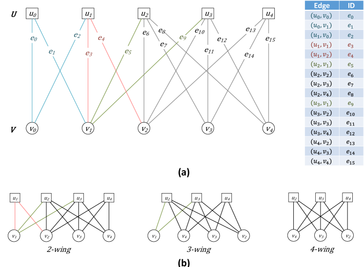
Figure 1. (a) Bipartite graph $G(U,V,E)$ which is also a $1$-wing. (b) Wing decomposition hierarchy of $G(U,V,E)$ – edges colored blue, red, green and black have wing numbers of 1, 2, 3 and 4, respectively.

Existing algorithms for decomposing bipartite graphs typically employ an iterative bottom-up peeling approach (sariyucePeeling, ; shiParbutterfly, ), wherein entities (edges and vertices for wing and tip decomposition, respectively) with the minimum support (butterfly count) are peeled in each iteration. Peeling an entity $l$ involves deleting it from the graph and updating the support of other entities that share butterflies with $l$. However, the huge number of butterflies in bipartite graphs makes bottom-up peeling computationally demanding and renders large graphs intractable for decomposing by sequential algorithms. For example, trackers – a bipartite network of internet domains and the trackers contained in them, has $140$ million edges but more than $20$ trillion butterflies.

Parallel computing is widely used to scale such high complexity analytics to large datasets (Park_2016, ; smith2017truss, ; 10.1145/3299869.3319877, ). However, the bottom-up peeling approach used in existing parallel frameworks (shiParbutterfly, ) severely restricts parallelism by peeling entities in a strictly increasing order of their entity numbers (wing or tip numbers). Consequently, it takes a very large number of iterations to peel an entire graph, for example, it takes $>31$ million iterations to peel all edges of the trackers dataset using bottom-up peeling. Moreover, each peeling iteration is sequentially dependent on support updates in all prior iterations, thus mandating synchronization of parallel threads before each iteration. Hence, the conventional approach of parallelizing workload within each iteration (shiParbutterfly, ) suffers from heavy thread synchronization, and poor parallel scalability.

In this paper, we propose a novel two-phased peeling approach for generalized bipartite graph decomposition. Both phases in the proposed approach exploit parallelism across multiple levels of the decomposition hierarchy to drastically reduce the number of parallel peeling iterations and in turn, the amount of thread synchronization. The first phase creates a coarse hierarchy which divides the set of entity numbers into few non-overlapping ranges. It accordingly partitions the entities by iteratively peeling the ones with support in the lowest range. A major implication of range-based partitioning is that each iteration peels a large number of entities corresponding to a wide range of entity numbers. This results in large parallel workload per iteration and little synchronization.

The second phase concurrently processes multiple partitions to compute the exact entity numbers. Absence of overlap between corresponding entity number ranges enables every partition to be peeled independently of others. By assigning each partition exclusively to a single thread, this phase achieves parallelism with no global synchronization.

We implement the two-phased peeling as a part of our Parallel Bipartite Network peelinG (PBNG) framework which adapts this approach for both wing and tip decomposition. PBNG further encapsulates novel workload optimizations that exploit batched peeling of numerous entities in the first phase to dramatically improve computational efficiency of decomposition. Overall, our contributions can be summarized as follows:

1. We propose a novel two-phased peeling approach for bipartite graph decomposition, that parallelizes workload across different levels of decomposition hierarchy. The proposed methodology is implemented in our PBNG framework which generalizes it for both vertex and edge peeling. To the best of our knowledge, this is the first approach to utilize parallelism across the levels of both wing and tip decomposition hierarchies.

2. Using the proposed two-phased peeling, we achieve a dramatic reduction in the number of parallel peeling iterations and in turn, the thread synchronization. As an example, wing decomposition of trackers dataset in PBNG requires only $2034$ parallel peeling iterations, which is four orders of magnitude less than existing parallel algorithms.

3. We develop novel optimizations that are highly effective for the two-phased peeling approach and dramatically reduce the work done by PBNG. As a result, PBNG traverses only $3.3$ trillion wedges during tip decomposition of internet domains in trackers dataset, compared to $211.1$ trillion wedges traversed by the state-of-the-art.

We empirically evaluate PBNG on several real-world bipartite graphs and demonstrate its superior scalability compared to state-of-the-art. We show that PBNG significantly expands the limits of current practice by decomposing some of the largest publicly available datasets in few minutes/hours, that existing algorithms cannot decompose in multiple days.

In a previous work (lakhotia2020receipt, ), we developed a two-phased algorithm for tip decomposition (vertex peeling). This paper generalizes the two-phased approach for peeling any set of entities within a bipartite graph. We further present non-trivial techniques to adopt the two-phased peeling for wing decomposition (edge peeling), which is known to reveal better quality dense subgraphs than tip decomposition (sariyucePeeling, ).

2. Background

In this section, we formally define the problem statement and review existing methods for butterfly counting and bipartite graph decomposition. Note that counting is used to initialize support (running count of butterflies) of each vertex or edge before peeling, and also inspires some optimizations to improve efficiency of decomposition.

Table 1 lists some notations used in this paper. For description of a general approach, we use the term entity to denote a vertex (for tip decomposition) or an edge (for wing decomposition), and entity number to denote tip or wing number (sec.2.2), respectively. Correspondingly, notations $\bowtie_{l}$ and $\theta_{l}$ denote the support and entity number of entity $l$.

Table 1. Notations and their definition

$G(W=(U,V),E)$	bipartite graph $G$ with disjoint vertex sets $U(G)$ and $V(G)$, and edges $E(G)$
$n/m$	no. of vertices in $G$ i.e. $n=|W|$ / no. of edges in $G$ i.e. $m=|E|$
$\alpha$	arboricity of $G$ (chibaArboricity, )
$N_{u}/d_{u}$	neighbors of vertex $u$ / degree of vertex $u$
$\bowtie_{u}^{G}$ / $\bowtie_{e}^{G}$	no. of butterflies in $G$ that contain vertex $u$ / edge $e$
$\bowtie_{u}$ / $\bowtie_{e}$	support (runing count of butterflies) of vertex $u$ / edge $e$
$\bowtie_{U}$ / $\bowtie_{E}$	support vector of all vertices in set $U(G)$ / all edges in $E(G)$
$\theta_{u}$ / $\theta_{e}$	tip number of vertex $u$ / wing number of edge $e$
$\theta^{max}_{U}$/$\theta^{max}_{E}$	maximum tip number of vertices in $U(G)$ / maximum wing number of edges in $E(G)$
$P$	number of vertex/edge partitions created by PBNG
$T$	number of threads

2.1. Butterfly counting

A butterfly (2,2-bicliques/quadrangle) can be viewed as a combination of two wedges with common endpoints. For example, in fig.1a, both wedges $(e_{0},e_{1})$ and $(e_{2},e_{3})$ have end points $v_{0}$ and $v_{1}$, and form a butterfly. A simple way to count butterflies is to explore all wedges and combine the ones with common end points. However, this is computationally inefficient with complexity $\mathcal{O}\left(\sum_{u\in U}\sum_{v\in N_{u}}d_{v}\right)=\mathcal{O}\left(\sum_{v\in V}d_{v}^{2}\right)$ (if we use vertices in $U$ as end points).

Chiba and Nishizeki (chibaArboricity, ) developed an efficient vertex-priority quadrangle counting algorithm in which starting from each vertex $u$, only those wedges are expanded where $u$ has the highest degree. It has a theoretical complexity of $\mathcal{O}\left(\sum_{(u,v)\in E}\min{(d_{u},d_{v})}\right)=\mathcal{O}\left(\alpha\cdot m\right)$, which is state-of-the-art for butterfly counting. Wang et al.(wangButterfly, ) further propose a cache-efficient version of this algorithm that traverses wedges such that the degree of the last vertex is greater than the that of the start and middle vertices (alg.1, line 10). Thus, wedge explorations frequently end at a small set of high degree vertices that can be cached.

The vertex-priority algorithm can be easily parallelized by concurrently processing multiple start vertices (shiParbutterfly, ; wangButterfly, ). In PBNG, we use the per-vertex and per-edge counting variants of the parallel algorithm (shiParbutterfly, ; wangButterfly, ), as shown in alg.1. To avoid conflicts, each thread is provided an individual $n$-element $wedge\_count$ array (alg.1, line 5) for wedge aggregation, and butterfly counts of entities are incremented using atomic operations.

Algorithm 1 Counting per-vertex and per-edge butterflies (pveBcnt)

1:Input: Bipartite Graph $G(W=(U,V),E)$

2:Output: Butterfly counts – $\bowtie_{u}$ for each $u\in W(G)$, and $\bowtie_{e}$ for each $e\in E(G)$

3:$\bowtie_{u}\ \leftarrow 0$ for each $u\in W(G)$;   $\bowtie_{e}\ \leftarrow 0$ for each $e\in E(G)$ $\triangleright$ Initialization

4:Relabel vertices $W(G)$ in decreasing order of degree$\triangleright$ Priority assignment

5:for each $u\in W(G)$ do in parallel

6:     Sort $N_{u}$ in increasing order of new labels

7:for each vertex $start\in W(G)$ do in parallel

8:     Initialize hashmap $wedge\_count$ to all zeros

9:     Initialize an empty wedge set $nzw\leftarrow\{\phi\}$

10:     for each vertex $mid\in N_{start}$

11:         for each vertex $last\in N_{mid}$

12:              if $(last\geq mid)$ or $(last\geq start)$ then break              

13:              $wedge\_count[last]\leftarrow wedge\_count[last]+1$

14:              $\ nzw\leftarrow nzw\cup(mid,last)$               

15:     for each $last$ such that $wedge\_count[last]>1$ $\triangleright$ Per-vertex counting

16:         $bcnt\leftarrow{wedge\_count[last]\choose 2}$

17:         $\bowtie_{start}\leftarrow\ \bowtie_{start}+\ bcnt$;   $\bowtie_{last}\leftarrow\ \bowtie_{last}+\ bcnt$

18:         for each $(mid,last)\in nzw$

19:              $\bowtie_{mid}\leftarrow\ \bowtie_{mid}+\ (wedge\_count[last]-1)$               

20:     for each $(mid,last)\in nzw$ such that $wedge\_count[last]>1$ $\triangleright$ Per-edge counting

21:         Let $e_{1}$ and $e_{2}$ denote edges $(start,mid)$ and $(mid,last)$, respectively

22:         $\bowtie_{e_{1}}\leftarrow\ \bowtie_{e_{1}}+\ (wedge\_count[last]-1)$;   $\bowtie_{e_{2}}\leftarrow\ \bowtie_{e_{2}}+\ (wedge\_count[last]-1)$      

2.2. Bipartite Graph Decomposition

Sariyuce et al.(sariyucePeeling, ) introduced $k-$tips and $k-$wings as a butterfly dense vertex and edge-induced subgraphs, respectively. They are formally defined as follows:

Definition 0.

A bipartite subgraph $H\subseteq G$, induced on edges $E(H)\subseteq E(G)$, is a k-wing iff

• each edge $e\in E(H)$ is contained in at least k butterflies,

• any two edges $(e_{1},e_{2})\in E^{\prime}$ is connected by a series of butterflies,

• $H$ is maximal i.e. no other $k-$wing in $G$ subsumes $H$.

Definition 0.

A bipartite subgraph $H\subseteq G$, induced on vertex sets $U(H)\subseteq U(G)$ and $V(H)=V(G)$, is a k-tip iff

• each vertex $u\in U(H)$ is contained in at least k butterflies,

• any two vertices $\{u,u^{\prime}\}\in U(H)$ are connected by a series of butterflies,

• $H$ is maximal i.e. no other $k-$tip in $G$ subsumes $H$.

Both $k-$wings and $k-$tips are hierarchical as a $k-$wing/$k-$tip completely overlaps with a $k^{\prime}-$wing/$k^{\prime}-$tip for all $k^{\prime}\leq k$. Therefore, instead of storing all $k-$wings, a wing number $\theta_{e}$ of an edge $e$ is defined as the maximum $k$ for which $e$ is present in a $k-$wing. Similarly, tip number $\theta_{u}$ of a vertex $u$ is the maximum $k$ for which $u$ is present in a $k-$tip. Wing and tip numbers act as a space-efficient indexing from which any level of the $k-$wing and $k-$tip hierarchy, respectively, can be quickly retrieved (sariyucePeeling, ). In this paper, we study the problem of finding wing and tip numbers, also known as wing and tip decomposition, respectively.

Bottom-Up Peeling (BUP) is a commonly employed technique to compute wing decomposition (alg.2). It initializes the support of each edge using per-edge butterfly counting (alg.2, line 1), and then iteratively peels the edges with minimum support until no edge remains. When an edge $e\in E$ is peeled, its support in that iteration is recorded as its wing number (alg.2, line 4). Further, for every edge $e^{\prime}$ that shares butterflies with $e$, the support $\bowtie_{e^{\prime}}$ is decreased corresponding to the removal of those butterflies. Thus, edges are peeled in a non-decreasing order of wing numbers.

Bottom-up peeling for tip decomposition utilizes a similar procedure for peeling vertices. A crucial distinction here is that in tip decomposition, vertices in only one of the sets $U(G)$ or $V(G)$ are peeled as a $k-$tip consists of all vertices from the other set (defn.2). For clarity of description, we assume that $U(G)$ is the vertex set to peel. As we will see later in sec.3.2, this distinction renders the two-phased approach of PBNG highly suitable for decomposition.

Runtime of bottom-up peeling is dominated by wedge traversal required to find butterflies that contain the entities being peeled (alg.2, lines 7-9). The overall complexity for wing decomposition is $\mathcal{O}\left(\sum_{(u,v)\in E(G)}\sum_{v\in N_{u}}d_{v}\right)=\mathcal{O}\left(\sum_{u\in U(G)}\sum_{v\in N_{u}}d_{u}d_{v}\right)$. Relatively, tip decomposition has a lower complexity of $\mathcal{O}\left(\sum_{u\in U(G)}\sum_{v\in N_{u}}d_{v}\right)=\mathcal{O}\left(\sum_{v\in V(G)}d_{v}^{2}\right)$, which is still quadratic in vertex degrees and very high in absolute terms.

Algorithm 2 Wing decomposition using bottom-up peeling (BUP)

1:Input: Bipartite graph $G(W=(U,V),E)$

2:Output: Wing numbers $\theta_{e}\ \forall\ e\in E(G)$

3:$\bowtie_{E}\ \leftarrow$ pveBcnt($G$)$\triangleright$ Counting for support initialization (alg.1)

4:while $E(G)\neq\ \{\phi\}$ do$\triangleright$ Peeling

5:     $e\leftarrow\arg\min_{e\in E(G)}\{\bowtie_{e}\}$

6:     $\theta_{e}\leftarrow\ \bowtie_{e},\ \ E(G)\leftarrow E(G)\setminus\{e\}$

7:     update($e,\theta_{e},\bowtie_{E},G$)

8:

9:function update($e=(u,v),\theta_{e},\bowtie_{E},G$)

10:     for each $v^{\prime}\in N_{u}\setminus\{v\}$$\triangleright$ Find butterflies

11:         Let $e_{1}$ denote edge $(u,v^{\prime})$

12:         for each $u^{\prime}\in N_{v^{\prime}}\setminus\{u\}$ such that $(u^{\prime},v)\in E(G)$

13:              Let $e_{2}$ and $e_{3}$ denote edges $(u^{\prime},v)$ and $(u^{\prime},v^{\prime})$, respectively

14:              $\bowtie_{e_{1}}\leftarrow\max\left(\theta_{e},\ \bowtie_{e_{1}}-1\right)$;   $\bowtie_{e_{2}}\leftarrow\max\left(\theta_{e},\ \bowtie_{e_{2}}-1\right)$;   $\bowtie_{e_{3}}\leftarrow\max\left(\theta_{e},\ \bowtie_{e_{3}}-1\right)$$\triangleright$ Update support               

2.3. Bloom-Edge-Index

Chiba and Nishizeki (chibaArboricity, ) proposed storing wedges derived from the computational patterns of their butterfly counting algorithm, as a space-efficient representation of all butterflies. Wang et al.(wangBitruss, ) used a similar representation termed Bloom-Edge-Index (BE-Index) for quick retrieval of butterflies containing peeled edges during wing decomposition. We extensively utilize BE-Index not just for computational efficiency, but also for enabling parallelism in wing decomposition. In this subsection, we give a brief overview of some key concepts in this regard.

The butterfly counting algorithm assigns priorities (labels) to all vertices in a decreasing order of their degree (alg.1, line 2). Based on these priorities, a structure called maximal priority $k-$bloom, which is the basic building block of BE-Index, is defined as follows (wangBitruss, ):

Definition 0.

A maximal priority $k-$bloom $B(W=(U,V),E)$ is a $(2,k)-$biclique (either $U(B)$ or $V(B)$ has exactly two vertices, each connected to all $k$ vertices in $V(B)$ or $U(B)$, respectively) that satisfies the following conditions:

1. The highest priority vertex in $W(B)$ belongs to the set ($U(B)$ or $V(B)$) which has exactly two vertices, and

2. $B$ is maximal i.e. there exists no $(2,k)-$biclique $B^{\prime}$ such that $B\subset B^{\prime}\subseteq G$ and $B^{\prime}$ satisfies condition $1$.

Maximal Priority Bloom Notations:

The vertex set ($U(B)$ or $V(B)$) containing the highest priority vertex is called the dominant set of $B$. Note that each vertex in the non-dominant set has exactly two incident edges in $E(B)$, that are said to be twins of each other in bloom $B$. For example, in the graph $G^{\prime}$ shown in fig.2, the subgraph induced on $\{v_{0},v_{1},u_{0},u_{1}\}$ is a maximal priority $2-$bloom with $v_{1}\in V(B)$ as the highest priority vertex and twin edge pairs $\{e_{0},e_{1}\}$ and $\{e_{2},e_{3}\}$. The twin of an edge $e$ in bloom $B$ is denoted by $twin(e,B)$. The cardinality of the non-dominant vertex set of bloom $B$ is called the bloom number of $B$. Wang et al.(wangBitruss, ) further prove the following properties of maximal priority blooms:

Property 1.

A $k-$bloom $B(W=(U,V),E)$ consists of exactly ${k\choose 2}=\frac{k*(k-1)}{2}$ butterflies. Each edge $e\in E(B)$ is contained in exactly $k-1$ butterflies in $B$. Further, edge $e$ shares all $k-1$ butterflies with $twin(e,B)$, and one butterfly each with all other edges $e^{\prime}\in E(B)\setminus\{twin(e,B)\}$.

Property 2.

A butterfly in $G$ must be contained in exactly one maximal priority $k-$bloom.

Note that the butterflies containing an edge $e$, and the other edges in those butterflies, can be obtained by exploring all blooms that contain $e$. For quick access to blooms of an edge and vice-versa, BE-Index is defined as follows:

Definition 0.

BE-Index of a graph $G(W=(U,V),E)$ is a bipartite graph $I(W=(U,V),E)$ that links all maximal priority blooms in $G$ to the respective edges within the blooms.

• W(I) – Vertices in $U(I)$ and $V(I)$ uniquely represent all maximal priority blooms in $G$ and edges in $E(G)$, respectively. Each vertex $B\in U(I)$ also stores the bloom number $k_{B}(I)$ of the corresponding bloom.

• E(I) – There exists an edge $(e,B)\in E(I)$ if and only if the corresponding bloom $B\subseteq G$ contains the edge $e\in E(G)$. Each edge $(e,B)\in E(I)$ is labeled with $twin(e,B)$.

BE-Index Notations:

For ease of explanation, we refer to a maximal priority bloom as simply bloom. We use the same notation $B$ (or $e$) to denote both a bloom (or edge) and its representative vertex in BE-Index. Neighborhood of a vertex $B\in U(I)$ and $e\in V(I)$ is denoted by $N_{B}(I)$ and $N_{e}(I)$, respectively. The bloom number of $B$ in BE-Index $I$ is denoted by $k_{B}(I)$. Note that $k_{B}(I)=\frac{\mathinner{\!\left\lvert N_{B}(I)\right\rvert}}{2}$.

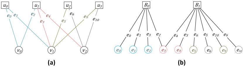
Figure 2. (a) Bipartite graph $G^{\prime}(W=(U,V),E)$ (b) BE-Index of $G^{\prime}$ with two maximal priority blooms.

Fig.2 depicts a graph $G^{\prime}$ (subgraph of $G$ from fig.1) and its BE-Index. $G^{\prime}$ consists of two maximal priority blooms: (a) $B_{0}$ with dominant set $V(B_{0})=\{v_{0},v_{1}\}$ and $k_{B_{0}}(I)=2$, and (b) $B_{1}$ with dominant vertex set $V(B_{1})=\{v_{1},v_{2}\}$ and $k_{B_{0}}(I)=3$. As an example, edge $e_{3}$ is a part of $1$ butterfly in $B_{0}$ shared with twin $e_{2}$, and $2$ butterflies in $B_{1}$ shared with twin $e_{4}$. With all other edges in $B_{0}$ and $B_{1}$, it shares one butterfly each.

Construction of BE-Index:

Index construction can be easily embedded within the counting procedure (alg.1). Each pair of endpoint vertices $\{start,last\}$ of wedges explored during counting, represents the dominating set of a bloom (with $last$ as the highest priority vertex) containing the edges $\{start,mid\}$ and $\{mid,last\}$ for all midpoints $mid$. Lastly, for a given vertex $mid$, edges $\{start,mid\}$ and $\{mid,last\}$ are twins of each other. Thus, the space and computational complexities of BE-Index construction are bounded by the the wedges explored during counting which is $\mathcal{O}\left(\alpha\cdot m\right)$.

Wing Decomposition with BE-Index:

Alg.3 depicts the procedure to peel an edge $e$ using BE-Index $I$. Instead of traversing wedges in $G$ to find butterflies of $e$, edges that share butterflies with $e$ are found by exploring 2-hop neighborhood of $e$ in $I$ (alg.3, line 7). Number of butterflies shared with these edges in each bloom is also obtained analytically using property 1 (alg.3, lines 4 and 8). Remarkably, peeling an edge $e$ using alg.3 requires at most $\bowtie_{e}^{G}$ traversal in BE-Index (wangBitruss, ). Thus, it reduces the computational complexity of wing decomposition to $\mathcal{O}\left(\sum_{e\in E(G)}\bowtie_{e}^{G}\right)$. However, it is still proportional to the number of butterflies which can be enormous for large graphs.

Algorithm 3 Support update during edge peeling, using BE-Index

1:function update($e,\theta_{e},\bowtie_{E},\text{BE-Index}\ I(W=(U,V),E)$)

2:     for each bloom $B\in N_{e}(I)$

3:         $e_{t}\leftarrow twin(e,B)$, $\ \ k_{B}(I)\leftarrow$ bloom number of $B$ in $I$

4:         $\bowtie_{e_{t}}\ \leftarrow\ \max\left(\theta_{e},\ \bowtie_{e_{t}}-\ (k_{B}(I)-1)\right)$

5:         $E(I)\leftarrow E(I)\setminus\{(e,B),(e_{t},B)\}$

6:         $k_{B}(I)\leftarrow k_{B}(I)-1$$\triangleright$ Update bloom number

7:         for each $e^{\prime}\in N_{B}(I)$

8:              $\bowtie_{e^{\prime}}\leftarrow\max\{\theta_{e},\ \bowtie_{e^{\prime}}-1\}$$\triangleright$ Update support               

2.4. Challenges

Bipartite graph decomposition is computationally very expensive and parallel computing is widely used to accelerate such workloads. However, state-of-the-art parallel framework ParButterfly (shiParbutterfly, ; julienne, ) is based on bottom-up peeling and only utilizes parallelism within each peeling iteration. This restricted parallelism is due to the following sequential dependency between iterations – support updates in an iteration guide the choice of entities to peel in the subsequent iterations. Hence, even though ParButterfly is work-efficient (shiParbutterfly, ), its scalability is limited because:

1. It incurs large number of iterations and low parallel workload per iteration. Due to the resulting synchronization and load imbalance, intra-iteration parallelism is insufficient for substantial acceleration.
   Objective 1 is therefore, to design a parallelism aware peeling methodology for bipartite graphs that reduces synchronization and exposes large amount of parallel workload.

2. It traverses an enormous amount of wedges (or bloom-edge links in BE-Index) to retrieve butterflies removed by peeling. This is computationally expensive and can be infeasible on large datasets, even for a parallel algorithm.
   Objective 2 is therefore, to reduce the amount of traversal in practice.

3. Parallel Bipartite Network peelinG (PBNG)

In this section, we describe a generic parallelism friendly two-phased peeling approach for bipartite graph decomposition (targeting objective $1$, sec.2.4). We further demonstrate how this approach is adopted individually for tip and wing decomposition in our Parallel Bipartite Network peelinG (PBNG) framework.

3.1. Two-phased Peeling

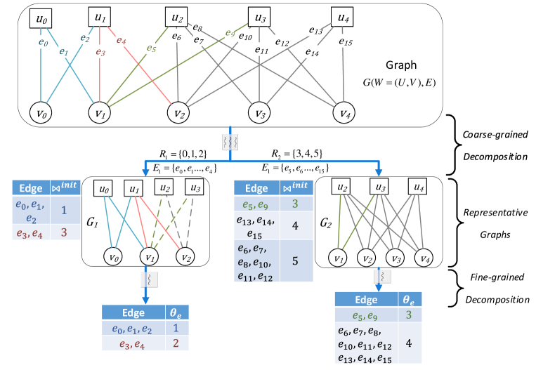
Figure 3. Graphical illustration of PBNG’s two-phased peeling for wing decomposition of the graph $G$ from fig.1. The coarse-grained decomposition divides $E(G)$ into $P=2$ partitions using parallel peeling iterations. The fine-grained decomposition peels each partition using a single thread but concurrently processes multiple partitions.

The fundamental observation underlining our approach is that entity number $\theta_{l}$ for an entity $l$ only depends on the number of butterflies shared between $l$ and other entities with entity numbers no less than $\theta_{l}$. Therefore, given a graph $G(W=(U,V),E)$ and per-entity butterfly counts in $G$ (obtained from counting), only the cumulative effect of peeling all entities with entity number strictly smaller than $\theta_{l}$, is relevant for computing $\theta_{l}-$level ($\theta_{l}-$tip or $\theta_{l}-$wing) in the decomposition hierarchy. Due to commutativity of addition, the order of peeling these entities has no impact on $\theta_{l}-$level.

This insight allows us to eliminate the constraint of deleting only minimum support entities in each iteration, which bottlenecks the available parallelism. To find $\theta_{l}-$level, all entities with entity number less than $\theta_{l}$ can be peeled concurrently, providing sufficient parallel workload. However, for every possible $\theta_{l}$, peeling all entities with smaller entity number will be computationally very inefficient. To avoid this inefficiency, we develop a novel two-phased approach.

3.1.1. Coarse-grained Decomposition

The first phase divides the spectrum of all possible entity numbers $[0,\theta^{max}]$ into $P$ smaller non-overlapping ranges ${R_{1},R_{2}\dots R_{P}}$, where $\theta^{max}$ is the maximum entity number in $G$, and $P$ is a user-specified parameter. A range $R_{i}$ represents a set of entity numbers $[\theta(i),\theta(i+1))$, such that $R_{i}\cap R_{j}=\{\phi\}$ for all $j\neq i$. These ranges are computed using a heuristic described in sec.3.1.3. Corresponding to each range $R_{i}$, PBNG also computes the partition $L_{i}$ comprising all entities whose entity numbers lie in $R_{i}$. Thus, instead of finding the exact entity number $\theta_{l}$ of an entity $l$, the first phase of PBNG computes bounds on $\theta_{l}$. Therefore, we refer to this phase as Coarse-grained Decomposition (PBNG CD). The absence of overlap between the ranges allows each subset to be peeled independently of others in the second phase, for exact entity number computation.

Entity partitions are computed by iteratively peeling entities whose support lie in the minimum range (alg.4,lines 5-13). For each partition, the first peeling iteration in PBNG CD scans all entities to find the peeling set, denoted as $activeSet$ (alg.4, line 9). In subsequent iterations, $activeSet$ is computed jointly with support updates. Thus, unlike bottom-up peeling, PBNG CD does not require a priority queue data structure which makes support updates relatively cheaper.

PBNG CD can be visualized as a generalization of bottom-up peeling (alg.2). In each iteration, the latter peels entities with minimum support ($\mathinner{\!\left\lvert R_{i}\right\rvert}=1$ for all $i$), whereas PBNG CD peels entities with support in a broad custom range ($\mathinner{\!\left\lvert R_{i}\right\rvert}\geq 1$). For example, in fig.3, PBNG CD divides edges $E(G)$ into two partitions corresponding to ranges $R_{1}=[0,2]$ and $R_{2}=[3,5]$, whereas bottom-up peeling will create $4$ partitions corresponding to every individual level in the decomposition hierarchy ($\theta=\{1,2,3,4\}$). Setting $P\ll\theta^{max}$ ensures a large number of entities peeled per iteration (sufficient parallel workload) and significantly fewer iterations (dramatically less synchronization) compared to bottom-up peeling.

In addition to the ranges and partitions, PBNG CD also computes a support initialization vector $\bowtie^{init}$. For an entity $l\in L_{i}$, $\bowtie^{init}_{l}$ is the number of butterflies that $l$ shares only with entities in partitions $L_{j}$ such that $j\geq i$. In other words, it represents the aggregate effect of peeling entities with entity number in ranges lower than $R_{i}$. During iteative peeling in PBNG CD, this number is inherently generated after the last peeling iteration of $R_{i-1}$ and copied into $\bowtie^{init}(l)$ (alg.4, lines 6-7). For example, in fig.3, support of $e_{5}$ after peeling $E_{1}=\{e_{0},e_{1},e_{2},e_{3},e_{4}\}$ is $3$, which is recorded in $\bowtie^{init}_{e_{5}}$.

Algorithm 4 PBNG Coarse-grained Decomposition (PBNG CD) for wing decomposition

1:Input: Bipartite graph $G(W=(U,V),E)$, # partitions $P$

2:Output: Ranges $\{\theta(1),\theta(2)\dots\theta(P+1)\}$, Edge Partitions $\{E_{1},E_{2}\dots E_{P}\}$, Support initialization vector $\bowtie^{init}_{E}$

3:$E_{i}\leftarrow\{\phi\}\ \forall\ i\in\{1,2\dots P\}$

4:Initial support $\{\bowtie_{E}\}\leftarrow$ pveBcnt($G$)$\triangleright$ Ref: alg.1

5:$I(W=(U,V),E)\leftarrow$ BE-Index of $G$

6:$\theta(1)\leftarrow 0$, $\ i\leftarrow 1$, $\ tgt\leftarrow$ target butterflies (workload) per partition

7:while $\left(E(G)\neq\ \{\phi\}\right)$ and $\left(i\leq P\right)$ do

8:     for each $e\in E(G)$ do in parallel$\triangleright$ Support Initialization Vector

9:         $\bowtie^{init}_{e}\leftarrow\ \bowtie_{e}$      

10:     $\theta(i+1)\leftarrow\text{{{find\_range}(}}E(G),\ \bowtie_{E},\ tgt\text{{)}}$$\triangleright$ Upper Bound

11:     $activeSet\leftarrow$ all edges $e\in E(G)$ such that $\ \theta(i)\leq\ \bowtie_{e}\ <\theta(i+1)$

12:     while $activeSet\neq\{\phi\}$ do$\triangleright$ Peel edges

13:         $E_{i}\leftarrow E_{i}\cup activeSet$, $\ E(G)\leftarrow E(G)\setminus activeSet$

14:         parallel_update($activeSet,\ \theta(i),\ \bowtie_{E},\ I$)

15:         $activeSet\leftarrow$ all edges $e\in E(G)$ such that $\ \theta(i)\leq\ \bowtie_{e}\ <\theta(i+1)$      

16:     $i\leftarrow i+1$

17:

18:function find_range($E(G),\ \bowtie_{E},\ tgt$)

19:     Initialize hashmap $work$ to all zeros

20:     for each $\theta\ \in\ \bowtie_{E}$

21:         $work[\theta]\leftarrow\sum_{e\in E(G)}\left(\bowtie_{e}\cdot\mathds{1}(\bowtie_{e}\leq\ \theta)\right)$      

22:     $\theta_{ub}\leftarrow$ $\arg\min\left(\theta\right)$ such that $work[\theta]\geq tgt$

23:     return $\theta_{ub}+1$

24:

25:function parallel_update($activeSet,\ \theta_{e},\ \bowtie_{E},\ \text{BE-Index}\ I(W=(U,V),E)$)

26:     Initialize hashmap $count$ to all zeros

27:     for each edge $e\in activeSet$ do in parallel

28:         for each bloom $B\in N_{e}(I)$$\triangleright$ Update support atomically

29:              $e_{t}\leftarrow twin(e,B)$, $\ \ k_{B}(I)\leftarrow$ bloom number of $B$ in $I$

30:              if $\left(e_{t}\notin activeSet\right)$ or $\left(edgeID(e_{t})<edgeID(e)\right)$ then

31:                  $\bowtie_{e_{t}}\ \leftarrow\ \max\left(\theta_{e},\ \bowtie_{e_{t}}-\ (k_{B}(I)-1)\right)$

32:                  $E(I)\leftarrow E(I)\setminus\{(e,B),(e_{t},B)\}$

33:                  $count[B]\leftarrow count[B]+1$

34:                  for each $e^{\prime}\in N_{B}(I)\$ such that $\ twin(e^{\prime},B)\notin activeSet$

35:                       $\bowtie_{e^{\prime}}\leftarrow\max\{\theta_{e},\ \bowtie_{e^{\prime}}-1\}$                                               

36:     for each $B\in U(I)$ such that $count[B]>0$ do in parallel

37:         $k_{B}(I)\leftarrow k_{B}(I)-count[B]$$\triangleright$ Update bloom number      

3.1.2. Fine-grained Decomposition

The second phase computes exact entity numbers and is called Fine-grained Decomposition (PBNG FD). The key idea behind PBNG FD is that if we have the knowledge of all butterflies that each entity $l\in L_{i}$ shares only with entities in partitions $L_{j}$ such that $j\geq i$, $L_{i}$ can be peeled independently of all other partitions. The $\bowtie^{init}$ vector computed in PBNG CD precisely indicates the count of such butterflies (sec.3.1.1) and hence, is used to initialize support values in PBNG FD. PBNG FD exploits the resulting independence among partitions to concurrently process multiple partitions using sequential bottom up peeling. Setting $P\gg T$ ensures that PBNG FD can be efficiently parallelized across partitions on $T$ threads. Overall, both phases in PBNG circumvent strict sequential dependencies between different levels of decomposition hierarchy to efficiently parallelize the peeling process.

The two-phased approach can potentially double the computation required for peeling. However, we note that since partitions are peeled independently in PBNG FD, support updates are not communicated across the partitions. Therefore, to improve computational efficiency, PBNG FD operates on a smaller representative subgraph $G_{i}\subseteq G$ for each partitions $L_{i}$. Specifically, $G_{i}$ preserves a butterfly $\bowtie$ iff it satisfies both of the following conditions:

1. $\bowtie$ contains multiple entities within $L_{i}$.

2. $\bowtie$ only contains entities from partitions $L_{j}$ such that $j\geq i$. If $\bowtie$ contains an entity from lower ranged partitions, then it does not exist in $\theta(i)$-level of decomposition hierarchy (lowest entity number in $L_{i}$). Moreover, the impact of removing $\bowtie$ on the support of entities in $L_{i}$, is already accounted for in $\bowtie^{init}$ (sec.3.1.1).

For example, in fig.3, $G_{1}$ contains the butterfly $\bowtie\ =\left(u_{1},v_{1},u_{2},v_{2}\right)$ because (a) it contains multiple edges $\{e_{3},e_{4}\}\in L_{1}$ and satisfies condition $1$, and (b) all edges in $\bowtie$ are from $L_{1}$ or $L_{2}$ and hence, it satisfies condition $2$. However, $G_{2}$ does not contain this butterfly because two if its edges are in $L_{1}$ and hence, it does not satisfy condition $2$ for $G_{2}$.

3.1.3. Range Partitioning

In PBNG CD, the first step for computing a partition $L_{i}$ is to find the range $R_{i}=[\theta(i),\theta(i+1))$ (alg.4, line 8). For load balancing, $\theta(i+1)$ should be computed such that the all partitions $L_{i}$ pose uniform workload in PBNG FD. However, the representative subgraphs and the corresponding workloads are not known prior to actual partitioning. Furthermore, exact entity numbers are not known either and hence, we cannot determine beforehand, exactly which entities will lie in $L_{i}$ for different values of $\theta(i+1)$. Considering these challenges, PBNG uses two proxies for range determination:

1. Proxy 1 $\rightarrow$ current support $\bowtie_{l}$ of an entity $l$ is used as a proxy for its entity number.

2. Proxy 2 $\rightarrow$ complexity of peeling individual entities in $G$ is used as a proxy to estimate peeling workload in representative subgraphs.

Now, the problem is to compute $\theta(i+1)$ such that estimated workload of $L_{i}$ as per proxies, is close to the average workload per partition denoted as $tgt$. To this purpose, PBNG CD creates a bin for each support value, and computes the aggregate workload of entities in that bin. For a given $\theta(i+1)$, estimated workload of peeling $L_{i}$ is the sum of workload of all bins corresponding to support less than $\theta(i+1)$. Thus, the workload of $L_{i}$ as a function of $\theta(i+1)$ can be computed by a prefix scan of individual bin workloads (alg.4, lines 17-18). Using this function, the upper bound is chosen such that the estimated workload of $L_{i}$ is close to but no less than $tgt$ (alg.4, line 19).

Adaptive Range Computation:

Since range determination uses current support as a proxy for entity numbers, the target workload for each partition $L_{i}$ is covered by the entities added to $L_{i}$ in its very first peeling iteration in PBNG CD. After the support updates in this iteration, more entities may be added to $L_{i}$ and final workload estimate of $L_{i}$ may significantly exceed $tgt$. This can result in significant load imbalance among the partitions and potentially, PBNG CD could finish in much fewer than $P$ partitions. To avoid this scenario, we implement the following two-way adaptive range determination:

1. Instead of statically computing an average target, we dynamically update $tgt$ for every partition based on the remaining workload and the number of partitions to create. If a partition gets too much workload, the target for subsequent partitions is automatically reduced, thereby preventing a situation where all entities get peeled in $\ll P$ partitions.

2. A partition $L_{i}$ likely covers many more entities than the initial estimate based on proxy 1. The second adaptation scales down the dynamic target for $L_{i}$ in an attempt to bring the actual workload close to the intended value. It assumes predictive local behavior i.e. $L_{i}$ will overshoot the target similar to $L_{i-1}$. Therefore, the scaling factor is computed as the ratio of initial workload estimate of $L_{i-1}$ during $\theta(i)$ computation, and final estimate based on all entities in $L_{i-1}$.

3.1.4. Partition scheduling in PBNG FD

While adaptive range determination(sec.3.1.3) tries to create partitions with uniform estimated workload, the actual workload per partition in PBNG FD depends on the the representative subgraphs $G_{i}$ and can still have significant variance. Therefore, to improve load balance across threads, we use scheduling strategies inspired from Longest Processing Time (LPT) scheduling rule which is a well known $\frac{4}{3}$-approximation algorithm (graham1969bounds, ). We use the workload of $L_{i}$ as an indicator of its execution time in the following runtime scheduling mechanism:

• Dynamic task allocation$\rightarrow$ All partition IDs are inserted in a task queue. When a thread becomes idle, it pops a unique ID from the queue and processes the corresponding partition. Thus, all threads are busy until every partition is scheduled.

• Workload-aware Scheduling$\rightarrow$ Partition IDs in the task queue are sorted in a decreasing order of their workload. Thus, partitions with highest workload get scheduled first and the threads processing them naturally receive fewer tasks in the future. Fig.4 shows how workload-aware scheduling can improve the efficiency of dynamic allocation.

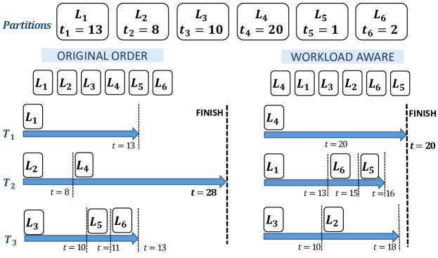
Figure 4. Benefits of Workload-aware Scheduling (WaS) in a $3$-thread ($T_{1},T_{2}$ and $T_{3}$) system. Top row shows entity partitions with estimated time to peel them in PBNG FD. Dynamic allocation without WaS finishes in $28$ units of time compared to $20$ units with WaS.

3.2. Tip Decomposition

In this section, we give a brief overview of PBNG’s two-phased peeling (sec.3.1) applied for tip decomposition. A detailed description of the same is provided in our previous work (lakhotia2020receipt, ).

For tip decomposition, PBNG CD divides the vertex set $U(G)$ into $P$ partitions – $\{U_{1},U_{2},\dots,U_{P}\}$. Peeling a vertex $u\in U(G)$ requires traversal of all wedges with $u$ as one of the endpoints. Therefore, range determination in PBNG CD uses wedge count of vertices in $G$, as a proxy to estimate the workload of peeling each partition $U_{i}$. Moreover, since only one of the vertex sets of $G$ is peeled, at most two vertices of a butterfly can be a part of the peeling set ($activeSet$). Hence, support updates to a vertex $u^{\prime}$ from different vertices in $activeSet$ correspond to disjoint butterflies in $G$. The net update to support $\bowtie_{u^{\prime}}$ can be simply computed by atomically aggregating the updates from individual vertices in $activeSet$.

PBNG FD also utilizes the fact that any butterfly $\bowtie$ contains at most two vertices $\{u,u^{\prime}\}$ in the vertex set $U(G)$ being peeled (sec.2.2). If $u\in U_{i}$ and $u^{\prime}\in U_{j}$, the two conditions for preserving $\bowtie$ in either representative graphs $G_{i}$ or $G_{j}$ are satisfied only when $i=j$ (sec.3.1.2). Based on this insight, we construct $G_{i}$ as the subgraph induced on vertices $W_{i}=(U_{i},V(G))$. Clearly, $G_{i}$ preserves every butterfly $\left(u,v,u^{\prime},v^{\prime}\right)$ where $\{u,u^{\prime}\}\in U_{i}$. For task scheduling in PBNG FD (sec.3.1.4), we use the total wedges in $G_{i}$ with endpoints in $U_{i}$ as an indicator of the workload of peeling $U_{i}$.

Given the bipartite nature of graph $G$, any edge $(u,v)\in E(G)$ exists in exactly one of the subgraphs $G_{i}$ and thus, the collective space requirement of all induced subgraphs is bounded by $O(m)$. Moreover, by the design of representative (induced) subgraphs, PBNG FD for tip decomposition traverses only those wedges for which both the endpoints are in the same partition. This dramatically reduces the amount of work done in PBNG FD compared to bottom-up peeling and PBNG CD. Note that we do not use BE-Index for tip decomposition due to the following reasons:

• Butterflies between two vertices are quadratic in the number of wedges between them, and wedge traversal (not butterfly count) determines the work done in tip decomposition. Since BE-Index facilitates per-edge butterfly retrieval, peeling a vertex using BE-Index will require processing each of its edge individually and can result in increased computation if $\sum_{v\in V(G)}d_{v}^{2}\ll\sum_{e\in E(G)}\bowtie_{e}^{G}$ (sec.2.3).

• BE-Index has a high space complexity of $\mathcal{O}\left(\sum_{(u,v)\in E(G)}\min{\left(d_{v},d_{u}\right)}\right)$ compared to just $\mathcal{O}\left(m\right)$ space needed to store $G$ and all induced subgraphs $G_{i}$. This can make BE-Index based peeling infeasible even on machines with large amount of main memory. For example, BE-Index of a user-group dataset Orkut ($327$ million edges) has $26$ billion blooms, $150$ billion bloom-edge links and consumes $2.6$ TB memory.

3.3. Wing Decomposition

3.3.1. Challenges

Each butterfly consists of $4$ edges in $E(G)$ which is the entity set to decompose in wing decomposition. This is unlike tip decomposition where each butterfly has only $2$ vertices from the decomposition set $U(G)$, and results in the following issues:

1. When a butterfly $\bowtie$ is removed due to peeling, the support of unpeeled edge(s) in $\bowtie$ should be reduced by exactly $1$ corresponding to this removal. However, when multiple (but not all) edges in $\bowtie$ are concurrently peeled in the same iteration of PBNG CD, multiple updates with aggregate value $>1$ may be generated to unpeeled edges in $\bowtie$.

2. It is possible that a butterfly $\bowtie$ contains multiple but not all edges from a partition. Thus, $\bowtie$ may need to be preserved in the representative subgraph of a partition, but will not be present in its edge-induced subgraph.

Due to these reasons, a trivial extension of tip decomposition algorithm (sec.3.2) is not suitable for wing decomposition. In this section, we explore novel BE-Index based strategies to enable two-phased peeling for wing decomposition.

3.3.2. PBNG CD

This phase divides the edges $E(G)$ into $P$ partitions – $\{E_{1},E_{2},\dots,E_{P}\}$, as shown in alg.4. Not only do we utilize BE-Index for computationally efficient support update computation in PBNG CD, we also utilize it to avoid conflicts in parallel peeling iterations of PBNG CD. Since a butterfly is contained in exactly one maximal priority bloom (sec.2.3, property 2), correctness of support updates within each bloom $B$ implies overall correctness of support updates in an iteration. To avoid conflicts, we therefore employ the following resolution mechanism for each bloom $B$:

1. If an edge $e$ and its twin $e^{\prime}=twin(e,B)$ are both peeled in the same iteration, then only the edge with highest index among $e$ and $e^{\prime}$ updates (a) the support of other edges in $B$, and (b) the bloom number $k_{B}(I)$ (alg.4, lines 26-31). This is because all butterflies in $B$ that contain $e$ also contain $e^{\prime}$ (sec.2.3, property1).

2. If in an iteration, an edge $e\in activeSet$ but $e^{\prime}=twin(e,B)\notin activeSet$, then the support $\bowtie_{e^{\prime}}$ is decreased by exactly ${k_{B}(I)-1}$ when $e$ is peeled. Other edges in $activeSet$ do not propagate any updates to $\bowtie_{e^{\prime}}$ via bloom $B$ (alg.4, lines 26-30). This is because $e^{\prime}$ is contained in exactly ${k_{B}(I)-1}$ butterflies in $B$, all of which are removed when $e$ is peeled. To ensure that $k_{B}(I)$ correctly represents the butterflies shared between twin edges, support updates from all peeled edges are computed prior to updating $k_{B}(I)$.

Peeling an edge $e\in E(G)$ requires $\mathcal{O}\left(\bowtie_{e}\right)$ traversal in the BE-Index. Therefore, range determination in PBNG CD uses edge support as a proxy to estimate the workload of peeling each partition $E_{i}$.

Algorithm 5 PBNG Fine-grained Decomposition (PBNG FD) for wing decomposition

1:Input: Graph $G(W=(U,V),E)$, BE-Index $I(W=(U,V),E)$, edge partitions $\{E_{1},\dots,E_{P}\}$

2:          Support initialization vector $\bowtie^{init}_{E}$

3:Output: Wing number $\theta_{e}$ for all $e\in E(G)$

4:$\bowtie_{e}\ \leftarrow\ \bowtie^{init}_{e}$ for all $e\in E_{i}$ $\triangleright$ Initialize Support

5:$\{I_{1},I_{2},\dots,I_{P}\}\leftarrow$ partition_BE_Index($G,I$)$\triangleright$ BE-Indices for all partitions

6:Insert integers $\{1,2,\dots,P\}$ in queue $Q$

7:Compute $work[i]\leftarrow\sum_{e\in E_{i}}{\bowtie_{e}^{init}\ }$ for all $i\in Q$, and sort $Q$ by $work$$\triangleright$ LPT Scheduling

8:for $thread\_id\in\{1,2\dots T\}$ do in parallel

9:     while $Q$ is not empty do

10:         Atomically pop integer $i$ from $Q$$\triangleright$ Dynamic Task Allocation

11:         while $E_{i}\neq\{\phi\}$ do$\triangleright$ Peel partition

12:              $e\leftarrow\arg\min_{e\in E_{i}}\{\bowtie_{e}\}$

13:              $\theta_{e}\leftarrow\ \bowtie_{e}$, $\ E_{i}\leftarrow E_{i}\setminus\{e\}$

14:              update($e,\theta_{e},\bowtie_{E_{i}},I_{i}$)$\triangleright$ Ref: alg.3               

15:

16:function partition_BE_Index($G(W=(U,V),E),I(W=(U,V),E)$)$\triangleright$ Compute partitions’ BE-Indices

17:     Let $p(e)$ denote the partition index of an edge $e$ i.e. $e\in E_{p(e)}$

18:     $V(I_{i})\leftarrow E_{i},\ U(I_{i})\leftarrow\{\phi\},\ E(I_{i})\leftarrow\{\phi\}\ \forall\ i\in\{1,2\dots P\}$

19:     for each $B\in U(I)$ do in parallel

20:         Initialize hash map $wedge\_count$ to all zeros

21:         for each $e\in N_{B}(I)$

22:              $e_{t}\leftarrow twin(e,B)$

23:              if $p(e_{t})\geq p(e)$ then

24:                  $U(I_{i})\leftarrow U(I_{i})\cup\{B\},\ \ E(I_{i})\leftarrow E(I_{i})\cup\left(e,B\right)$ $\triangleright$ Add bloom-edge links

25:                  if $\left(p(e_{t}))>p(e)\right)$ or $\left(edgeID(e_{t})<edgeID(e)\right)$ then$\triangleright$ Initialize bloom numbers

26:                       $wedge\_count(I_{i})\leftarrow wedge\_count(I_{i})+1$                                          

27:         for each partition index $i$ such that $B\in U(I_{i})$

28:              $k_{B}(I_{i})\leftarrow\sum_{j\geq i}{wedge\_count(I_{j})}$$\triangleright$ Compute bloom numbers (prefix scan)               

29:     return $\{I_{1},I_{2},\dots,I_{P}\}$

3.3.3. PBNG FD

The first step for peeling a partition $E_{i}$ in PBNG FD, is to construct the corresponding BE-Index $I_{i}$ for its representative subgraph $G_{i}$. One way to do so is to compute $G_{i}$ and then use the index construction algorithm (sec.2.3) to construct $I_{i}$. However, this approach has the following drawbacks:

• Computing $G_{i}$ requires mining all edges in $E(G)$ that share butterflies with edges $e\in E_{i}$, which can be computationally expensive. Additionally, the overhead of index construction even for a few hundred partitions can be significantly large.

• Any edge $e\in E_{i}$ can potentially exist in all subgraphs $G_{j}$ such that $j\leq i$. Therefore, creating and storing all subgraphs $G_{i}$ requires $\mathcal{O}(mP)$ memory space.

To avoid these drawbacks, we directly compute $I_{i}$ for each $E_{i}$ by partitioning the BE-Index $I$ of the original graph $G$ (alg.5, lines 12-25). Our partitioning mechanism ensures that all butterflies satisfying the two preservation conditions (sec.3.1.2) for a partition $E_{i}$, are represented in its BE-Index $I_{i}$.

Firstly, for an edge $e\in E_{i}$, its link $(e,B)$ with a bloom $B$ is preserved in $I_{i}$ if and only if the twin $e_{t}=twin(e,B)\in E_{j}$ such that $j\geq i$ (alg.5, lines 19-20). Since all butterflies in $B$ that contain $e$ also contain $e_{t}$ (sec.2.3, property 1), none of them need to be preserved in $I_{i}$ if $j<i$. Moreover, if $\{e,e_{t}\}\in E_{i}$, their contribution to the bloom number $k_{B}(I_{i})$ is counted only once (alg.5, lines -22).

Secondly, for a space-efficient representation, $I_{i}$ does not store a link $\left(e^{\prime},B\right)$ if $e^{\prime}\notin E_{i}$. However, while such an edge $e^{\prime}$ will not participate in peeling of $E_{i}$, it may be a part of a butterfly in $B$ that satisfies both preservation conditions for $I_{i}$ (sec.3.1.2). For example, fig.2 shows the representative subgraph $G_{1}$ and BE-Index for the partition $E_{1}$ generated by PBNG CD in fig.3. For space efficiency, we do not store the links $\{(e_{5},B_{1}),(e_{6},B_{1}),(e_{9},B_{1}),(e_{10},B_{1})\}$ in $I_{1}$. However, the two butterflies in $B_{1}$ – $(e_{3},e_{4},e_{5},e_{6})$ and $(e_{3},e_{4},e_{9},e_{10})$, satisfy both preservation conditions for $I_{1}$, and may be needed when peeling $e_{3}$ or $e_{4}$. In order to account for such butterflies, we adjust the bloom number $k_{B}(I_{i})$ to correctly represent the number of butterflies in $B$ that only contain edges from all partitions $E_{j}$ such that $j\geq i$ (alg.5, lines 23-24). For example, in fig.2b, we initialize the bloom number of $B_{1}$ to $k_{B_{1}}(I_{1})=3$ even though $\mathinner{\!\left\lvert N_{B_{1}}(I_{1})\right\rvert}=2$. Thus, $k_{B_{1}}(I_{1})$ correctly represents the ${3\choose 2}=3$ butterflies in $B_{1}$, that contain edges only from $\cup_{j\geq 1}\{E_{j}\}$ .

After the BE-Indices for partitions are computed, PBNG FD dynamically schedules partitions on threads, where they are processed using sequential bottom-up peeling. Here, the aggregate initial support of a partition’s edges (given by $\bowtie^{init}_{E}$ vector) is used as an indicator of its workload (alg.5, line 4) for LPT scheduling  (sec.3.1.2).

4. Analysis

4.1. Correctness of Decomposition Output

In this section, we prove the correctness of wing numbers and tip numbers computed by PBNG. We will exploit comparisons with sequential BUP (alg.2) and hence, first establish the follwing lemmas:

Lemma 0.

In BUP, the support $\bowtie_{e}$ of an edge $e$ at any time $t$ before the first edge with wing number $\geq\theta_{e}$ is peeled, depends on the cumulative effect of all edges peeled till $t$ and is independent of the order in which they are peeled.

Proof.

Let $\bowtie_{e}^{G}$ denote the number of butterflies in $G$ that contain $e$, $S$ be the set of vertices peeled till time $t$ and $\bowtie_{e,e_{a},e_{b},e_{c}}$ denote a butterfly containing $e$ and other edges $\{e_{a},e_{b},e_{c}\}$ such that $a>b>c$ (for uniqueness of representation). If $e_{a}$, $e_{b}$ or $e_{c}$ are peeled till $t$, corresponding to the removal of $\bowtie_{e,e_{a},e_{b},e_{c}}$, only one of them (the first edge to be peeled) reduces the support $\bowtie_{e}$ by a unit. Since BUP peels edges in a non-decreasing order of their wing numbers, $\theta_{e^{\prime}}<\theta_{e}$ for all $e^{\prime}\in S$. Hence, current support (alg.2, line 11) of $e$ is given by $\bowtie_{e}\ =\ \bowtie_{e}^{G}-\sum_{\bowtie_{e,e_{a},e_{b},e_{c}}}{\mathds{1}(e_{a}\in S\ \texttt{or}\ e_{b}\in S\ \texttt{or}\ e_{c}\in S)}$. The first term of RHS is constant for a given $G$, and by commutativity of addition, the second term is independent of the order in which contribution of individual butterflies are added. Therefore, $\bowtie_{e}$ is independent of the order of peeling in $S$. ∎

Lemma 0.

Given a set $S$ of edges peeled in an iteration, the parallel peeling in PBNG CD (alg.4, lines 21-33) correctly updates the support of remaining edges in $E(G)$.

Proof.

Parallel updates are correct if for an edge $e$ not yet assigned to any partition, $\bowtie_{e}$ decreases by exactly $1$ for each butterfly of $e$ deleted in a peeling iteration. By property 2 (sec.2.3), parallel updates are correct if this holds true for butterflies deleted within each bloom.

Consider a bloom $B(W=(U,V),E)$ and let $\bowtie_{e,e_{t},e^{\prime},e^{\prime}_{t}}\subseteq B$ be a butterfly containing edges $\{e,e_{t},e^{\prime},e^{\prime}_{t}\}$, where $e_{t}=twin(e,B)$ and $e^{\prime}_{t}=twin(e^{\prime},B)$ (property 1, sec.2.3), such that $\bowtie_{e,e_{t},e^{\prime},e^{\prime}_{t}}$ is deleted in the $j^{th}$ peeling iteration of PBNG CD. Clearly, neither of $e$, $e_{t}$, $e^{\prime}$ or $e^{\prime}_{t}$ have been peeled before $j^{th}$ iteration. We analyze updates to support $\bowtie_{e}$ corresponding to the deletion of butterfly $\bowtie_{e,e_{t},e^{\prime},e^{\prime}_{t}}$. If $S$ denotes the set of edges peeled in $j^{th}$ iteration, $\bowtie$ will be deleted if and only if either of the following is true:

1. $e\in S\rightarrow$ In this case, $e$ is already assigned to a partition and updates to $\bowtie_{e}$ have no impact on the output of PBNG.

2. $e\notin S$ but $e_{t}\in S\rightarrow$ $\bowtie_{e}$ is reduced by exactly $(k_{B}-1)$ via bloom $B$, which amounts to unit reduction per each butterfly in $B$ that contains $e$ (property 1, sec.2.3). No updates from other edges are propagated to $\bowtie_{e}$ via $B$ (alg.4, line 30).

3. $\{e,e_{t}\}\notin S$ but $e^{\prime}\in S$ or $e^{\prime}_{t}\in S$ $\rightarrow$ $\bowtie_{e}$ is decreased by exactly $1$ when $e^{\prime}/e^{\prime}_{t}$ is peeled. If both $\{e^{\prime},e^{\prime}_{t}\}\in S$, then $\bowtie_{e}$ is decreased by exactly $1$ when the highest indexed edge among $e^{\prime}$ and $e^{\prime}_{t}$ is peeled (alg.4, line 26). Both the links $(e^{\prime},B)$ and $(e^{\prime}_{t},B)$ are deleted and bloom number $k_{B}$ is decreased by $1$. Hence, subsequent peeling of any edges will not generate support updates corresponding to $\bowtie_{e,e_{t},e^{\prime},e^{\prime}_{t}}$.

Thus, the removal of $\bowtie$ during peeling decreases the support of $e$ by exactly $1$ if $e$ is not scheduled for peeling yet. ∎

Lemmas 1 and 2 together show that whether we peel a set $S\subseteq E(G)$ in its original order in BUP, or in parallel in any order in PBNG CD, the support of edges with wing numbers higher than all edges in $S$ would be the same after peeling $S$. Next, we show that PBNG CD correctly computes the edge partitions corresponding to wing number ranges and finally prove that PBNG FD outputs correct wing numbers for all edges. For ease of explanation, we use $\bowtie_{e}(j)$ to denote the support of a edge $e$ after $j^{th}$ peeling iteration in PBNG CD.

Lemma 0.

There cannot exist an edge $e$ such that $e\in E_{i}$ and $\theta_{e}\geq\theta(i+1)$.

Proof.

Let $j$ be the first iteration in PBNG CD that wrongly peels a set of edges $S_{w}$, and assigns them to $E_{i}$ even though $\theta_{e}\geq\theta(i+1)\ \forall\ e\in S_{w}$. Let $S_{hi}\supseteq S_{w}$ be the set of all edges with wing numbers $\geq\theta(i+1)$ and $S_{lo}$ be the set of edges peeled till iteration $j-1$. Since all edges till $j-1$ iterations have been correctly peeled, $\theta_{e}<\theta(i+1)\ \forall\ e\in S_{lo}$. Hence, $S_{hi}\subseteq E(G)\setminus S_{lo}$.

Consider an edge $e\in S_{w}$. Since $e$ is peeled in $j^{th}$ iteration, ${\bowtie_{e}(j-1)}<\theta(i+1)$. From lemma 2, $\bowtie_{e}(j-1)$ is equal to the number of butterflies containing $e$ and edges only from $E\setminus S_{lo}$. Since $S_{hi}\subseteq E(G)\setminus S_{lo}$, there are at most $\bowtie_{e}(j-1)$ butterflies that contain $e$ and other edges only from $S_{hi}$. By definition of wing number (sec.2.2), $\theta_{e}\leq\bowtie_{e}(j-1)<\theta(i+1)$, which is a contradiction. Thus, no such $e$ exists, $S_{w}=\{\phi\}$, and all edges in $E_{i}$ have tip numbers less than $\theta(i+1)$. ∎

Lemma 0.

There cannot exist an edge $e$ such that $e\in E_{i}$ and $\theta_{e}<\theta(i)$.

Proof.

Let $R_{i}$ be the smallest range for which there exists an edge $e$ such that $\theta(i)\leq\theta_{e}<\theta(i+1)$, but $e\in E_{i^{\prime}}$ for some $i^{\prime}>i$. Let $j$ be the last peeling iteration in PBNG CD that assigns edges to $E_{i}$, and $S_{hi}=\cup_{i^{\prime}>i}E_{i^{\prime}}$ denote the set of edges not peeled till this iteration. Clearly, $e\in S_{hi}$ and for each edge $e^{\prime}\in S_{hi}$, $\bowtie_{e^{\prime}}(j)\geq\theta(i+1)$, otherwise $e^{\prime}$ would be peeled in or before the $j^{th}$ iteration. From lemma 2, all edges in $S_{hi}$ (including $e$) participate in at least $\theta(i+1)$ butterflies that contain edges only from $S_{hi}$. Therefore, $e$ is a part of $\theta(i+1)-wing$ (def.1) and by the definition of wing number, $\theta_{e}\geq\theta(i+1)$, which is a contradiction. ∎

Theorem 5.

PBNG CD (alg.4) correctly computes the edge partitions corresponding to every wing number range.

Proof.

Follows directly from lemmas 3 and 4. ∎

Theorem 6.

PBNG correctly computes the wing numbers for all $e\in E(G)$.

Proof.

From theorem 5, $\theta(i)\leq\theta_{e}<\theta(i+1)$ for each edge $e\in E_{i}$. Consider an edge partition $E_{i}$ and Let $S_{lo}=E_{1}\cup E_{2}\dots E_{i-1}$ denote the set of edges peeled before $E_{i}$ in PBNG CD. From theorem 5, $\theta_{e}\geq\theta(i)$ for all edges $e\in E_{i}$, and $\theta_{e}<\theta(i)$ for all edges $e\in S_{lo}$. Hence, $S_{lo}$ will be peeled before $E_{i}$ in BUP as well. Similarly, any edge in $S_{hi}=E_{i+1}\cup E_{i+2}\dots\cup E_{P}$ will be peeled after $E_{i}$ in BUP. Hence, support updates to any edge $e\in S_{hi}$ have no impact on wing numbers computed for edges in $E_{i}$.

For each edge $e\in E_{i}$, PBNG FD initializes $\bowtie_{e}$ using $\bowtie^{init}_{e}$, which is the support of $e$ in PBNG CD just after $S_{lo}$ is peeled. From lemma 2, this is equal to the support of $e$ in BUP just after $S_{lo}$ is peeled.

Note that both PBNG FD and BUP employ same algorithm (sequential bottom-up peeling) to peel edges in $E_{i}$. Hence, to prove the correctness of wing numbers generated by PBNG FD, it suffices to show that when an edge in $E_{i}$ is peeled, support updates propagated to other edges in $E_{i}$ via each bloom $B$, are the same in PBNG FD and BUP.

1. Firstly, every bloom-edge link $(e,B)$ where $e\in E_{i}$ and $twin(e,B)\in E_{i}\cup S_{hi}$, is preserved in the partition’s BE-Index $I_{i}$. Thus, when an edge $e\in E_{i}$ is peeled, the set of affected edges in $E_{i}$ are correctly retrieved from $I_{i}$ (same as the set retrieved from BE-Index $I$ in BUP).

2. Secondly, by construction (alg.5, lines 21-22 and 23-24), the initial bloom number of $B$ in $I_{i}$ is equal to the number of those twin edge pairs in $B$, for which both edges are in $E_{i}$ or higher ranged partitions (not necessarily in same partition). Thus, $k_{B}(I_{i})=\frac{\sum_{e\in E(B)}{\mathds{1}\left(\theta_{e}\geq\theta(i)\ \texttt{and}\ \theta_{twin(e,B)}\geq\theta_{i}\right)}}{2}$, which in turn is the bloom number $k_{B}(I)$ in BUP just before $E_{i}$ is peeled.

Since both PBNG FD and BUP have identical support values just before peeling $E_{i}$, the updates computed for edges in $E_{i}$ and the order of edges peeled in $E_{i}$ will be the same as well. Hence, the final wing numbers computed by PBNG FD will be equal to those computed by BUP. ∎

The correctness of tip decomposition in PBNG can be proven in a similar fashion. A detailed derivation for the same is given in theorem $2$ of (lakhotia2020receipt, ),

4.2. Computation and Space Complexity

To feasibly decompose large datasets, it is important for an algorithm to be efficient in terms of computation and memory requirements. The following theorems show that for a reasonable upper bound on partitions $P$, PBNG is at least as computationally efficient as the best sequential decomposition algorithm BUP.

Theorem 7.

For $P=\mathcal{O}\left(\frac{\sum_{e\in E(G)}{\bowtie_{e}^{G}}}{m}\right)$ partitions, wing decomposition in PBNG is work-efficient with computational complexity of $\mathcal{O}\left(\alpha\cdot m+\sum_{e\in E(G)}{\bowtie_{e}^{G}}\right)$, where $\bowtie_{e}^{G}$ is the number of butterflies in $G$ that contain $e$.

Proof.

PBNG CD initializes the edge support using butterfly counting algorithm with ${\mathcal{O}\left(\alpha\cdot m\right)}$ complexity. Since $\theta^{max}_{E}\leq m$, binning for range computation of each partition can be done using an $\mathcal{O}(m)$-element array, such that $i^{th}$ element in the array corresponds to workload of edges with support $i$ (alg.4, lines 16-19). A prefix scan of the array gives the range workload as a function of the upper bound. Parallel implementations of binning and prefix scan perform $\mathcal{O}(m)$ computations per partition, amounting to $\mathcal{O}\left(P\cdot m\right)$ computations in entire PBNG CD. Constructing $activeSet$ for first peeling iteration of each partition requires an $\mathcal{O}(m)$ complexity parallel filter on remaining edges. Subsequent iterations construct $activeSet$ by tracking support updates doing $\mathcal{O}(1)$ work per update. Further, peeling an edge $e$ generates $\mathcal{O}(\bowtie_{e}^{G})$ updates, each of which can be applied in constant time using BE-Index (sec.2.3). Therefore, total complexity of PBNG CD is $\mathcal{O}\left(\sum_{e\in E(G)}{\bowtie_{e}^{G}}+(P+\alpha)\cdot m\right)$.

PBNG FD partitions BE-Index $I$ to create individual BE-Indices for edge partitions. The partitioning (alg.5, lines 12-25) requires constant number of traversals of entire set $E(I)$ and hence, has a complexity of $\mathcal{O}(\alpha\cdot m)$. Each butterfly in $G$ is represented in at most one partition’s BE-Index. Therefore, PBNG FD will also generate $\mathcal{O}\left(\sum_{e\in E(G)}{\bowtie_{e}^{G}}\right)$ support updates. Hence, the work complexity of PBNG FD is $\mathcal{O}\left(\sum_{e\in E(G)}{\bowtie_{e}^{G}}+\alpha\cdot m\right)$ (sec.2.3).

The total work done by PBNG is $\mathcal{O}\left(\sum_{e\in E(G)}{\bowtie_{e}^{G}}+(P+\alpha)\cdot m\right)=\mathcal{O}\left(\sum_{e\in E(G)}{\bowtie_{e}^{G}}+\alpha\cdot m\right)$ if $P=\mathcal{O}\left(\frac{\sum_{e\in E(G)}{\bowtie_{e}^{G}}}{m}\right)$, which is the best-known time complexity of BUP. Hence, PBNG’s wing decomposition is work-efficient. ∎

Theorem 8.

For $P=\mathcal{O}\left(\frac{\sum_{u\in U}\sum_{v\in N_{u}}{d_{v}}}{n\log{n}}\right)$ partitions, tip decomposition in PBNG is work-efficient with computational complexity of $\mathcal{O}\left(\sum_{u\in U}\sum_{v\in N_{u}}{d_{v}}\right)$.

Proof.

The proof is simliar to that of theorem 7. The key difference from wing decomposition is that maximum tip number can be cubic in the size of the vertex set. Therefore, range determination uses a hashmap with support values as the keys. The aggregate workloads of the bins need to be sorted on keys before computing the prefix scan. Hence, total complexity of range determination for tip decomposition in PBNG CD is $\mathcal{O}\left(P\cdot n\log{n}\right)$. A detailed derivation is given in theorem $3$ of (lakhotia2020receipt, ). ∎

Next, we prove that PBNG’s space consumption is almost similar to the best known sequential algorithms.

Theorem 9.

Wing decomposition in PBNG parallelized over $T$ threads consumes $\mathcal{O}\left(\alpha\cdot m+n\cdot T\right)$ memory space.

Proof.

For butterfly counting, each thread uses a private $\mathcal{O}(n)$ array to accumulate wedge counts, resulting to $\mathcal{O}(n\cdot T)$ space consumption (wangButterfly, ). For peeling:

1. PBNG CD uses the BE-Index $I(W=(U,V),E)$ whose space complexity is $\mathcal{O}\left(\alpha\cdot m\right)$.

2. PBNG FD uses individual BE-Indices for each partition. Any bloom-edge link $(e,B)\in E(I)$ exists in at most one partition’s BE-Index. Therefore, cumulative space required to store all partitions’ BE-Indices is $\mathcal{O}\left(\alpha\cdot m\right)$.

Thus, overall space complexity of PBNG’s wing decomposition is $\mathcal{O}\left(\alpha\cdot m+n\cdot T\right)$. ∎

Theorem 10.

Tip decomposition in PBNG parallelized over $T$ threads consumes $\mathcal{O}\left(m+n\cdot T\right)$ memory space.

Proof.

For butterfly counting and peeling in PBNG, each thread uses a private $\mathcal{O}(n)$ array to accumulate wedge counts, resulting in $\mathcal{O}(n\cdot T)$ space consumption. In PBNG FD, any edge $e\in E(G)$ exists in the induced subgraph of at most one partition (because partitions of $U(G)$ are disjoint). Hence, $\mathcal{O}\left(n+m\right)$ space is required to store $G$ and all induced subgraphs, resulting in overall $\mathcal{O}\left(m+n\cdot T\right)$ space complexity. ∎

5. Optimizations

Despite the use of parallel computing resources, PBNG may consume a lot of time to decompose large graphs such as the trackers dataset, that contain several trillion wedges (for tip decomposition) or butterflies (for wedge decomposition). In this section, we propose novel optimization techniques based on the two-phased peeling of PBNG, that dramatically improve computational efficiency and make it feasible to decompose datasets like trackers in few minutes.

5.1. Batch Processing

Due to the broad range of entity numbers peeled in each iteration of PBNG CD (sec.3.1.1), some iterations may peel a large number of entities. Peeling individual entities in such iterations requires a large amount of traversal in $G$ or BE-Index $I$. However, visualizing such iterations as peeling a single large set of entities can enable batch optimizations that drastically reduce the required computation.

Tip Decomposition

Here, we exploit the fact that (per-vertex) butterfly counting is computationally efficient and parallelizble (sec.2.1). Given a vertex set $activeSet$, the number of wedges traversed for peeling $activeSet$ is given by $\wedge(activeSet)=\sum_{u\in activeSet}{\sum_{v\in N_{u}}d_{v}}$. However, number of wedges traversed for re-counting butterflies for remaining vertices is upper bounded by $\wedge_{cnt}=\sum_{(u,v)\in E}\min\left(d_{u},d_{v}\right)$, which is constant for a given $G$ (sec.2.1). If $\wedge(activeSet)>\wedge_{cnt}$, we re-compute butterflies for all remaining vertices in $U$ instead of peeling $activeSet$. Thus, computational complexity of a peeling iteration in PBNG tip decomposition is $\mathcal{O}\left(\alpha\cdot m\right)$.

Algorithm 6 Batch computation of support updates from peeling a set of edges $activeSet$

1:function update($activeSet,\theta_{e},\bowtie_{E},\text{BE-Index}\ I(W=(U,V),E)$)

2:     Initialize hashmap $count$ to all zeros

3:     for each edge $e\in activeSet$ do in parallel

4:         for each bloom $B\in N_{e}(I)$

5:              $e_{t}\leftarrow twin(e,B),\ \ k_{B}(I)\leftarrow$ bloom number of $B$ in $I$

6:              if $\left(e_{t}\notin activeSet\right)$ or $\left(edgeID(e_{t})<edgeID(e)\right)$ then

7:                  $\bowtie_{e_{t}}\ \leftarrow\ \max\left(\theta_{e},\ \bowtie_{e_{t}}-\ k_{B}(I)\right)$

8:                  $count[B]\leftarrow count[B]+1$$\triangleright$ Aggregate updates at blooms atomically

9:                  $E(I)\leftarrow E(I)\setminus\{(e,B),(e_{t},B)\}$                             

10:     for each bloom $B\in U(I)$ such that $count[B]>0$ do in parallel

11:         $k_{B}(I)\leftarrow k_{B}(I)-count[B]$$\triangleright$ Update bloom number

12:         for each edge $e^{\prime}\in N_{B}(I)$

13:              $\bowtie_{e^{\prime}}\leftarrow\max\{\theta_{e},\ \bowtie_{e^{\prime}}-count[B]\}$$\triangleright$ Update support atomically               

Wing Decomposition

For peeling a large set of edges $activeSet$, we use the batch processing proposed in (wangBitruss, ). The key idea is that when an edge $e$ is peeled, the affected edges are discovered by exploring the neighborhood of blooms in $N_{e}(I)$ (alg.3). Therefore, the support updates from all edges in $activeSet$ can be aggregated at the blooms (alg.6, line 8), and then applied via a single traversal of their neighborhoods (alg.6, lines 10-13). Thus, computational complexity of a peeling iteration in PBNG wing decomposition is bounded by the size of BE-Index which is $\mathcal{O}\left(\alpha\cdot m\right)$. While batch processing using BE-Index was proposed in (wangBitruss, ), we note that it is significantly more beneficial for PBNG CD compared to bottom-up peeling, due to the large number of edges peeled per iteration.

5.2. Dynamic Graph Updates

After a vertex $u$ (or an edge $e$) is peeled in PBNG, it is excluded from future computation in the respective phase. However, due to the undirected nature of the graph, the adjacency list data structure for $G$ (or BE-Index $I$) still contains edges of $u$ (or bloom-edge links of $e$) that are interleaved with other edges. Consequently, wedges incident on $u$ (or bloom-edge links of $e$), though not used in computation, are still explored even after $u$ (or $e$) is peeled. To prevent such wasteful exploration, we update the data structures to remove edges incident on peeled vertices (or bloom-edge links of peeled edges).

These updates can be performed jointly with the traversal required for peeling. In tip decomposition, updating vertex support requires traversing adjacencies of the neighbors of peeled vertices. Edges to peeled vertices can be removed while traversing neighbors’ adjacency lists. In wing decomposition, updating edge support requires iterating over the affected blooms (alg.6, lines 10-13) and their neighborhoods $N_{B}(I)$. The bloom-edge links incident on peeled edges and their twins can be removed from $N_{B}(I)$ during such traversal.

6. Experiments

In this section, we present detailed experimental results of PBNG for both tip and wing decomposition. In sec.6.1, we list the datasets and describe the baselines used for comparison. Secondly, in sec.6.2, we provide a thorough evaluation of wing decomposition in PBNG. We (a) compare PBNG against the baselines on several metrics, (b) report empirical benefits of optimizations proposed in sec.5, (c) compare workload and execution time of coarse and fine decomposition phases, and (d) evaluate parallel scalability of PBNG. Lastly, in sec.6.3, we report a similar evaluation of tip decomposition.

6.1. Setup

We conduct the experiments on a 36 core dual-socket linux server with two Intel Xeon E5-2695 v4 processors@ 2.1GHz and 1TB DRAM. All algorithms are implemented in C++-14 and are compiled using G++ 9.1.0 with the -O3 optimization flag, and OpenMP v4.5 for multithreading.

Datasets: We use twelve unweighted bipartite graphs obtained from the KOBLENZ collection (konect, ) and Network Repository (rossi2015network, ), whose characteristics are shown in table 2. To the best of our knowledge, these are some of the largest publicly available real-world bipartite datasets.

Table 2. Bipartite graphs with the corresponding number of butterflies ($\bowtie_{G}$ in billions), maximum tip numbers $\theta^{max}_{U}$ (for peeling $U$) and $\theta^{max}_{V}$ (for peeling $V$), and maximum wing number $\theta^{max}_{E}$.

Dataset	Description	$\mathbf{\mathinner{\!\left\lvert U\right\rvert}}$	$\mathbf{\mathinner{\!\left\lvert V\right\rvert}}$	$\mathbf{\mathinner{\!\left\lvert E\right\rvert}}$	$\mathbf{\boldsymbol{\bowtie}_{G}}$(in B)	$\mathbf{\boldsymbol{\theta}^{max}_{U}}$	$\mathbf{\boldsymbol{\theta}^{max}_{V}}$	$\mathbf{\boldsymbol{\theta}^{max}_{E}}$
Di-af	Artists and labels affiliation from Discogs	1,754,824	270,772	5,302,276	3.3	120,101,751	87,016,404	15,498
De-ti	URLs and tags from www.delicious.com	4,006,817	577,524	14,976,403	22.9	565,413	409,807,620	26,895
Fr	Pages and editors from French Wikipedia	62,890	94,307	2,494,939	34.1	1,561,397	645,790,738	54,743
Di-st	Artists and release styles from Discogs	1,617,944	384	5,740,842	77.4	736,089	1,828,291,442	52,015
It	Pages and editors from Italian Wikipedia	2,255,875	137,693	12,644,802	298	1,555,462	5,328,302,365	166,785
Digg	Users and stories from Digg	872,623	12,472	22,624,727	1,580.5	47,596,665	3,725,895,816	166,826
En	Pages and editors from English Wikipedia	21,504,191	3,819,691	122,075,170	2,036	37,217,466	96,241,348,356	438,728
Lj	Users’ group memberships in Livejournal	3,201,203	7,489,073	112,307,385	3,297	4,670,317	82,785,273,931	456,791
Gtr	Documents and words from Gottron-trec	556,078	1,173,226	83,629,405	19,438	205,399,233	38,283,508,375	563,244
Tr	Internet domains and trackers in them	27,665,730	12,756,244	140,613,762	20,068	18,667,660,476	3,030,765,085,153	2,462,017
Or	Users’ group memberships in Orkut	2,783,196	8,730,857	327,037,487	22,131	88,812,453	29,285,249,823	-
De-ut	Users and tags from www.delicious.com	4,512,099	833,081	81,989,133	26,683	936,468,800	91,968,444,615	1,290,680

Baselines: We compare the performance of PBNG against the following baselines:

• BUP$\rightarrow$ sequential bottom-up peeling (alg.2) that does not use BE-Index.

• ParB$\rightarrow$ParButterfly framework with the best performing BatchS aggregation method (shiParbutterfly, ). It parallelizes each iteration of BUP using a parallel bucketing structure (julienne, ).

• BE_Batch (for wing decomposition only)$\rightarrow$ BE-Index assisted peeling with batch processing optimization (wangBitruss, ), and dynamic deletion of bloom-edge links (sec.5).

• BE_PC (for wing decomposition only)$\rightarrow$ BE-Index assisted progressive compression peeling approach, proposed in (wangBitruss, ). It generates candidate subgraphs top-down in the hierarchy to avoid support updates from peeling edges in lower subgraphs (small $\theta_{e}$) to edges in higher subgraphs (high $\theta_{e}$). Scaling parameter for support threshold of candidate subgraphs is set to $\tau=0.02$, as specified in (wangBitruss, ).

Furthermore, to evaluate the effect of optimizations (sec.5), we create two variants of PBNG:

• PBNG- $\rightarrow$ PBNG without dynamic graph updates (sec.5.2).

• PBNG– $\rightarrow$ PBNG without dynamic graph updates (sec.5.2) and batch processing optimization (sec.5.1).

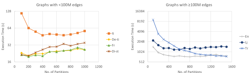
Figure 5. Execution time of wing decomposition vs number of partitions $P$ in PBNG.

Parameter Setting: The only user-specified parameter in PBNG is the no. of partitions $P$. For tip decomposition, we use $P=150$ which was empirically determined in (lakhotia2020receipt, ). For wing decomposition, we measure the runtime of PBNG as a function of $P$ as shown in fig.5. Performance of PBNG CD improves with a decrease in $P$ because of reduced peeling iterations and larger peeling set (batch size) per iteration. However, for PBNG FD, a small value of $P$ reduces parallelism and increases the workload. Thus, $P$ represents a trade-off between the two phases of PBNG. Based on our our observations, we set $P=400$ for graphs with $<100$ M edges, and $P=1000$ for graphs with $\geq 100$ M edges. We also note that the performance of PBNG is robust (within $2\times$ of the optimal) in a wide range of $P$ for both small and large datasets.

6.2. Results: Wing Decomposition

6.2.1. Comparison with Baselines

Table 3 shows a detailed comparison of PBNG and baseline wing decomposition algorithms. To compare the workload of different algorithms, we measure the number of support updates applied in each algorithm (wangBitruss, ). Note that this may under-represent the workload of BUP and ParB, as they cannot retrieve affected edges during peeling in constant time. However, it is a useful metric to compare BE-Index based approaches (wangBitruss, ) as support updates represent bulk of the computation performed by during decomposition.

Amongst the baseline algorithms, BE_PC demonstrates state-of-the-art execution time and lowest computational workload, represented by the number of support updates, due to its top-down subgraph construction approach. However, with the two-phased peeling and batch optimizations, support updates in PBNG are at par or even lower than BE_PC in some cases. Moreover, most updates in PBNG are applied to a simple array and are relatively cheaper compared to updates applied to priority queue data structure in all baselines (including BE_PC). Furthermore, by utilizing parallel computational resources, PBNG achieves up to $38.5\times$ speedup over BE_PC, with especially high speedup on large datasets.

Compared to the parallel framework ParB, PBNG is two orders of magnitude or more (up to $295\times$) faster. This is because ParB does not use BE-Index for efficient peeling, does not utilize batch optimizations to reduce computations, and requires large amount of parallel peeling iterations ($\rho$). The number of threads synchronizations is directly proportional to $\rho$, and PBNG achieves up to $15260\times$ reduction in $\rho$ compared to ParB. This is primarily because PBNG CD peels vertices with a broad range of support in every iteration, and PBNG FD does not require a global thread synchronization at alll. This drastic reduction in $\rho$ is the primary contributor to PBNG’s parallel efficiency.

Quite remarkably, PBNG is the only algorithm to successfully wing decompose Gtr and De-ut datasets in few hours, whereas all of the baselines fail to decompose them in two days. Overall, PBNG achieves dramatic reduction in workload, execution time and synchronization compared to all previously existing algorithms.

Table 3. Comparing execution time ($\mathbf{t}$), number of support updates and thread synchronization (or parallel peeling iterations $\rho$) for PBNG and baseline algorithms. Missing entries denote that execution did not finish in $2$ days. ParB will generate same number of support updates as BUP, and parallel variants of all baselines will have same amount of synchronization ($\rho$) as ParB.

		Di-af	De-ti	Fr	Di-st	It	Digg	En	Lj	Gtr	Tr	De-ut
	BUP	911	6,622	2,565	9,972	38,579	-	-	-	-	-	-
	ParB	324	3,105	1,434	2,976	14,087	-	-	-	-	-	-
	BE_Batch	87	568	678	961	9,940	-	78,847	-	-	54,865	-
	BE_PC	56	312	237	314	1756	37,006	25,905	50,901	-	28,418	-
$\mathbf{t}$(s)	PBNG	7.1	22.4	20.4	26.5	47.7	960	748	1,293	13,253	858	6,661
	BUP	4.7	37.3	39.4	122	424	-	-	-	-	-	-
	BE_Batch	2.9	16.6	24.8	33.9	119.0	1,413	1,116	-	-	679	-
	BE_PC	1.1	5.7	7.6	9.9	33.6	592	391	785	-	390	-
Updates (billions)	PBNG	1.9	9	11	11.6	26.9	794	402	678	5,765	164	5,530
	ParB	179,177	868,527	181,114	1,118,178	781,955	1,077,389	8,456,797	4,338,205	3,655,765	31,043,711	4,844,812
$\mathbf{\rho}$	PBNG	3,666	5,902	4,062	4,442	4,037	14,111	16,324	19,824	18,371	2,034	15,136

6.2.2. Effect of Optimizations

Since dynamic BE-Index updates do not affect the updates generated during peeling, PBNG and PBNG- exhibit the same number of support updates. Hence, to highlight the benefits of BE-Index updates (sec.5.2), we also measure the number of bloom-edge links traversed in PBNG with and without the optimizations. Fig.6 shows the effect of optimizations on the performance of PBNG.

Normalized performance of PBNG- (fig.6) shows that deletion of bloom-edge links (corresponding to peeled edges) from BE-Index reduces traversal by an average of $1.4\times$, and execution time by average $1.11\times$. However, traversal is relatively inexpensive compared to support updates as the latter involve atomic computations on array elements (PBNG CD) or on a priority queue (PBNG FD). Fig.6 also clearly shows a direct correlation between the execution time of PBNG– and the number of support updates. Consequently, the performance is drastically impacted by batch processing, without which large datasets Gtr, Tr and De-ut can not be decomposed in two days by PBNG–. Normalized performance of PBNG– shows that both optimizations cumulatively enable an average reduction of $9.1\times$ and $21\times$ in the number of support updates and execution time of wing decomposition, respectively. This shows that the two-phased approach of PBNG is highly suitable for batch optimization as it peels large number of edges per parallel iteration.

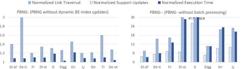
Figure 6. Effect of optimizations (sec.5) on wing decomposition in PBNG. All quantities are normalized with respective measurements for PBNG with all optimizations enabled. With batch processing disabled (PBNG–), Gtr, Tr and De-ut did not finish within $2$ days.

6.2.3. Comparison of Different Phases

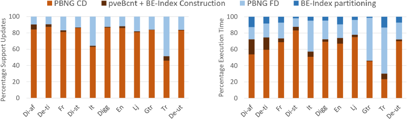
Figure 7. Contribution of different steps to the overall support updates and the execution time of wing decomposition in PBNG

Fig.7 shows a breakdown of the support updates and execution time of PBNG across different steps, namely initial butterfly counting and BE-Index Construction, peeling in PBNG CD, BE-Index partitioning and peeling in PBNG FD. For most datasets, PBNG CD dominates the overall workload, contributing more than $60\%$ of the support updates for most graphs. In some datasets such as Tr and Gtr, the batch optimizations drastically reduce the workload of PBNG CD, rendering PBNG FD as the dominant phase. The trends in execution time are largely similar to those of support updates. However, due to differences in parallel scalability of different steps, contribution of PBNG FD to execution time of several datasets is slightly higher than its corresponding contribution to support updates. We also observe that peeling in PBNG CD and PBNG FD is much more expensive compared to BE-Index construction and partitioning.

6.2.4. Scalability

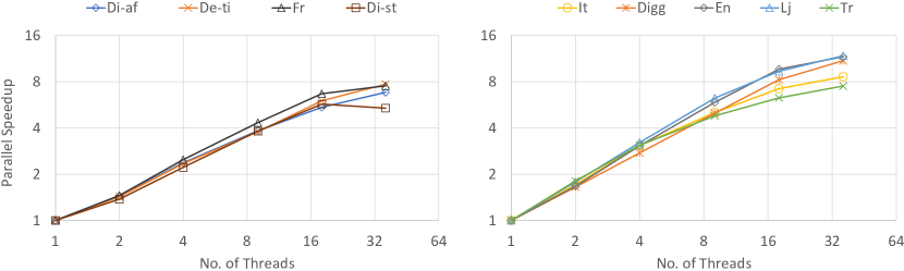
Figure 8. Strong scaling of wing decomposition in PBNG. Datasets shown on the left were decomposed in less than a minute, and on the right take several minutes.

Fig.8 demonstrates the parallel speedup of PBNG over sequential execution. Overall, PBNG provides an average $8.7\times$ parallel speedup with $36$ threads, which is significantly better than ParB. Furthermore, the speedup is generally higher for large datasets (up to $11.8\times$ for Lj), which are highly time consuming. Contrarily, ParB achieves an average $2.6\times$ speedup over sequential BUP, due to the large amount of synchronization.

We also observe that PBNG consistently accelerates decomposition up to $18$ threads (single socket), providing average $7.2\times$ parallel speedup. However, scaling to two sockets (increasing threads from $18$ to $36$) only fetches $1.2\times$ speedup on average. This could be due to NUMA effects which increases the cost of memory accesses and atomics. This can significantly impact the performance as PBNG’s workload is dominated by traversal of the large BE-Index and atomic support updates. Further, edges contained in a large number of butterflies may receive numerous support updates, which increases coherency traffic and reduces scalability.

6.3. Results: Tip Decomposition

To evaluate tip decomposition in PBNG, we select $6$ of the largest datasets from table 2 and individually decompose both vertex sets in them. Without loss of generality, we label the vertex set with higher peeling complexity as $U$ and the other as $V$. Corresponding to the set being decomposed, we suffix the dataset name with $U$ or $V$.

6.3.1. Comparison with Baselines

Table 4. Comparing execution time ($t$), # wedges traversed and # synchronization rounds (or parallel peeling iterations $\rho$) of PBNG and baseline algorithms for tip decomposition. ParB traverses the same # wedges as BUP and has missing entries due to out-of-memory error. BUP could not decompose TrU in $2$ days.

		EnU	EnV	LjU	LjV	GtrU	GtrV	TrU	TrV	OrU	OrV	De-utU	De-utV
	BUP	111,777	281	67,588	200	12,036	221	-	5,711	39,079	2,297	12,260	428
	ParB	-	198	-	132.5	-	163.9	-	3,524	-	1,510	-	377.7
$\mathbf{t}$(s)	PBNG	1,383	31.1	911.1	23.7	163.9	26.5	2,784	530.6	1,865	136	402.4	32.4
	BUP	12,583	29.6	5,403	14.3	3,183	26.6	211,156	1,740	4,975	231.4	2,861	70.1
Wedges (billions)	PBNG	2,414	22.2	1,003	11.7	1,526	28.2	3,298	658.1	2,728	170.4	1,503	51.3
	ParB	1,512,922	83,800	1,479,495	83,423	491,192	73,323	1,476,015	342,672	1,136,129	334,064	670,189	127,328
$\mathbf{\rho}$	PBNG	1,724	453	1,477	456	2,062	362	1,335	1,381	1,160	639	1,113	406

Table 4 shows a detailed comparison of various tip decomposition algorithms. To compare the workload of tip decomposition algorithms, we measure the number of wedges traversed in $G$. Wedge traversal is required to compute butterflies between vertex pairs during counting/peeling, and represents bulk of the computation performed in tip decomposition .

With up to $80.8\times$ and $64.7\times$ speedup over BUP and ParB, respectively, PBNG is dramatically faster than the baselines, for all datasets. Contrarily, ParB achieves a maximum $1.6\times$ speedup compared to sequential BUP for TrV dataset. The speedups are typically higher for large datasets that offer large amount of computation to parallelize and benefit more from batch optimization (sec.5.1).

Optimization benefits are also evident in the wedge traversal of PBNG. For all datasets, PBNG traverses fewer wedges than the baselines, achieving up to $64\times$ reduction in wedges traversed. Furthermore, PBNG achieves up to $1105\times$ reduction in synchronization ($\rho$) over ParB, due to its two-phased peeling approach. The resulting increase in parallel efficiency and workload optimizations enable PBNG to decompose large datasets like EnU in few minutes, unlike baselines that take few days for the same.

Quite remarkably, PBNG is the only algorithm to successfully tip decompose TrU dataset within an hour, whereas the baselines fail to decompose it in two days. We also note PBNG can decompose both vertex sets of Or dataset in approximately half an hour, even though none of the algorithms could feasibly wing decompose the Or dataset (sec.6.2). Thus, tip decomposition is advantageous over wing decomposition, in terms of efficiency and feasibility.

6.3.2. Optimizations

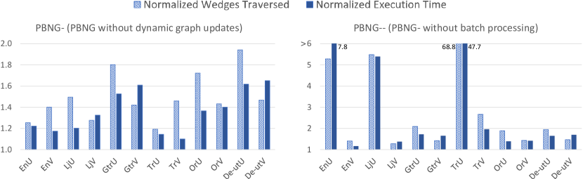
Figure 9. Effect of optimizations (sec.5) on tip decomposition in PBNG. All quantities are normalized with the respective measurements for PBNG with all optimizations enabled.

Fig.9 shows the effect of workload optimizations on tip decomposition in PBNG. Clearly, the execution time closely follows the variations in number of wedges traversed.

Dynamic deletion of edges (corresponding to peeled vertices) from adjacency lists can potentially half the wedge workload since each wedge has two endpoints in peeling set. Normalized performance of PBNG- (fig.6) shows that it achieves $1.41\times$ and $1.29\times$ average reduction in wedges and execution time, respectively.

Similar to wing decomposition, the batch optimization provides dramatic improvement in workload and execution time. This is especially true for datasets with a large ratio of total wedges with endpoints in peeling set to the wedges traversed during counting (for example, for LjU, EnU and TrU, this ratio is $>1000$). For instance, in TrU, both optimizations cumulatively enable $68.8\times$ and $47.7\times$ reduction in wedge traversal and execution time, respectively. Contrarily, in datasets with small value of this ratio such as DeV, OrV, LjV and EnV, none of the peeling iterations in PBNG CD utilize re-counting. Consequently, performance of PBNG- and PBNG– is similar for these datasets.

6.3.3. Comparison of phases

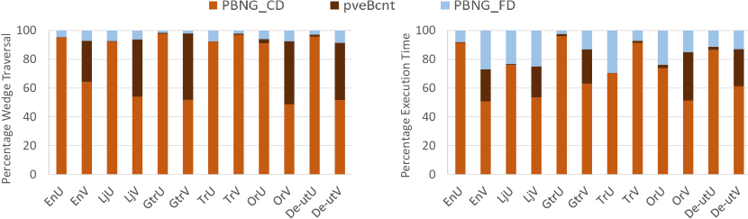
Figure 10. Contribution of different steps to the overall wedge traversal and the execution time of tip decomposition in PBNG

Fig.7 shows a breakdown of the wedge traversal and execution time of PBNG across different steps, namely initial butterfly counting, peeling in PBNG CD and PBNG FD. As expected, PBNG FD only contributes less than $15\%$ of the total wedge traversal in tip decomposition. This is because it operates on small subgraphs that preserve very few wedges of $G$. When peeling the large workload $U$ vertex set, more than $80\%$ of the wedge traversal and $70\%$ of the execution time is spent in PBNG CD.

6.3.4. Scalability

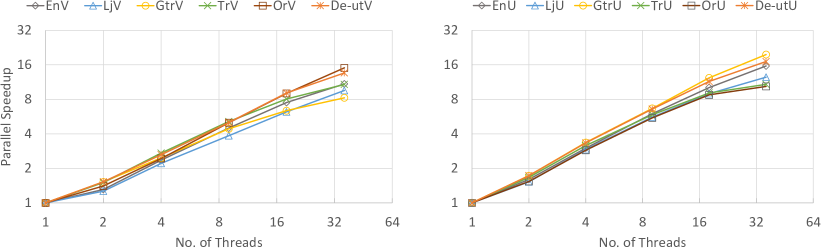
Figure 11. Strong scaling of tip decomposition in PBNG

Fig.11 demonstrates the parallel speedup of PBNG over sequential execution. When peeling the large workload vertex set $U$, PBNG achieves almost linear scalability with $14.4\times$ average parallel speedup on $36$ threads, and up to $19.7\times$ speedup for $GtrU$ dataset. Contrarily, ParB achieves an average $1.54\times$ speedup over sequential BUP, and up to $2.3\times$ speedup for $TrV$ dataset.

Typically, datasets with small amount of wedges (LjV, EnV) exhibit lower speedup, because they provide lower workload per synchronization round on average. For example, LjV traverses $86\times$ fewer wedges than LjU but incurs only $3.2\times$ fewer synchronizations. This increases the relative overheads of parallelization and restricts the parallel scalability of PBNG CD, which is the highest workload step in PBNG (fig.10). Similar to wing decomposition, NUMA effects on scalability to multiple sockets ($36$ threads) can be seen in tip decomposition of some datasets such as OrU and TrU. However, we still observe $1.4\times$ average speedup on large datasets when threads are increased from $18$ to $36$ threads. This is possibly because most of the workload in tip decomposition is comprised of wedge traversal which only reads the graph data structure. It incurs much fewer support updates, and in turn atomic writes, compared to wing decomposition.

7. Related Work

Discovering dense subgraphs and communities in networks is a key operation in several applications (anomalyDet, ; spamDet, ; communityDet, ; fang2020effective, ; otherapp1, ; otherapp2, ; nathan2017local, ; staudt2015engineering, ; riedy2011parallel, ). Motif-based techniques are widely used to reveal dense regions in graphs (sariyuce2016fast, ; fang2019efficient, ; gibson2005discovering, ; sariyuce2018local, ; angel2014dense, ; trussVLDB, ; lee2010survey, ; coreVLDB, ; coreVLDBJ, ; wang2018efficient, ; PMID:16873465, ; trussVLDB, ; tsourakakis2017scalable, ; tsourakakis2014novel, ; sariyucePeeling, ; aksoy2017measuring, ; wang2010triangulation, ). Motifs like triangles represent a quantum of cohesion in graphs and the number of motifs containing an entity (vertex or an edge) acts as an indicator of its local density. Consequently, several recent works have focused on efficiently finding such motifs in the graphs (green2018logarithmic, ; shun2015multicore, ; ahmed2015efficient, ; shiParbutterfly, ; wangButterfly, ; hu2018tricore, ; fox2018fast, ; ma2019linc, ).

Nucleus decomposition is a clique based technique for discovering hierarchical dense regions in unipartite graphs. Instead of per-entity clique count in the entire graph, it considers the minimum clique count of a subgraph’s entities as an indicator of that subgraph’s density (10.1007/s10115-016-0965-5, ). This allows mining denser subgraphs compared to counting alone (10.1007/s10115-016-0965-5, ; sariyuce2015finding, ). Truss decomposition is a special and one of the most popular cases of nucleus decomposition that uses triangle clique. It is a part of the GraphChallenge (samsi2017static, ) initiative, that has resulted in highly scalable parallel decomposition algorithms (date2017collaborative, ; voegele2017parallel, ; smith2017truss, ; green2017quickly, ). However, nucleus decomposition is not applicable on bipartite graphs as they do not have cliques.

The simplest non-trivial motif in a bipartite graph is a Butterfly (2,2-biclique). Several algorithms for butterfly counting have been developed: in-memory or external memory (wangButterfly, ; wangRectangle, ), exact or approximate counting (sanei2018butterfly, ; sanei2019fleet, ) and parallel counting on various platforms (shiParbutterfly, ; wangButterfly, ; wangRectangle, ). The most efficient approaches are based on Chiba and Nishizeki’s (chibaArboricity, ) vertex-priority butterfly counting algorithm. Wang et al.(wangButterfly, ) propose a cache optimized variant of this algorithm and use shared-memory parallelism for acceleration. Independently, Shi et al.(shiParbutterfly, ) develop provably efficient shared-memory parallel implementations of this algorithm. Notably, their algorithms are able to extract parallelism at the granularity of wedges explored. Such fine-grained parallelism can also be explored for improving parallel scalability of PBNG.

Inspired by $k$-truss, Sariyuce et al.(sariyucePeeling, ) defined $k$-tips and $k$-wings as subgraphs with minimum $k$ butterflies incident on every vertex and edge, respectively. Similar to nucleus decomposition algorithms, they designed bottom-up peeling algorithms to find hierarchies of $k$-tips and $k$-wings. Independently, Zou (zouBitruss, ) defined the notion of bitruss similar to $k$-wing. Shi et al.(shiParbutterfly, ) propose the $P\textsc{ar}B\textsc{utterfly}$ framework that parallelizes individual peeling iterations.

Chiba and Nishizeki (chibaArboricity, ) proposed that wedges traversed in butterfly counting algorithm can act as a space-efficient representation of all butterflies in the graph. Wang et al.(wangBitruss, ) propose a butterfly representation called BE-Index (also derived from the counting algorithm) for efficient support updates during edge peeling. Based on BE-Index, they develop several peeling algorithms for wing decomposition that achieve state-of-the-art computational efficiency and are used as baselines in this paper.

Very recently, Wang et al.(wang2021towards, ) also proposed parallel versions of BE-Index based wing decomposition algorithms. Although the code is not publicly available, authors report the performance on few graphs. Based on the reported results, PBNG significantly outperforms their parallel algorithms as well. Secondly, these algorithms parallelize individual peeling iterations and will incur heavy synchronization similar to $P\textsc{ar}B\textsc{utterfly}$ (table 3). Lastly, they are only designed for wing decomposition, whereas PBNG comprehensively targets both wing and tip decomposition. This is important because tip decomposition in PBNG (a) is typically faster than wing decomposition, and (b) can process large datasets like Orkut in few minutes, that none of the existing tip or wing decomposition algorithms can process in several days.

8. Conclusion and Future Work

In this paper, we studied the problem of bipartite graph decomposition which is a computationally demanding analytic for which the existing algorithms were not amenable to efficient parallelization. We proposed a novel parallelism friendly two-phased peeling framework called PBNG, that is the first to exploit parallelism across the levels of decomposition hierarchy. The proposed approach further enabled novel optimizations that drastically reduce computational workload, allowing bipartite decomposition to scale beyond the limits of current practice.

We presented a comprehensive empirical evaluation of PBNG on a shared-memory multicore server and showed that it can process some of the largest publicly available bipartite datasets two orders of magnitude faster than the state-of-the-art. PBNG also achieved a dramatic reduction in thread synchronization, allowing up to $19.7\times$ self-relative parallel speedup on $36$ threads.

There are several directions for future research in the context of this work. The proposed two-phased peeling can open up avenues for distributed-memory parallel bipartite decomposition on HPC clusters. Clusters allow scaling of both computational and memory resources, which is crucial for decomposing large graphs. To further improve the performance of PBNG, we will also explore fine-grained parallelism, and techniques to avoid atomics and enhance memory access locality. Such system optimizations have been shown to be highly effective in conventional graph processing frameworks (shun2013ligra, ; lakhotia2020gpop, ; zhang2018graphit, ). We believe that two-phased peeling could also benefit nucleus decomposition in unipartite graphs, which is an interesting direction to explore.

Acknowledgement

This material is based on work supported by the Defense Advanced Research Projects Agency (DARPA) under Contract Number FA8750-17-C-0086, and National Science Foundation (NSF) under Grant Numbers CNS-2009057 and OAC-1911229. Any opinions, findings and conclusions or recommendations expressed in this material are those of the authors and do not necessarily reflect the views of DARPA or NSF. The U.S. Government is authorized to reproduce and distribute reprints for Government purposes notwithstanding any copyright notation here on.

References

- (1) Ahmed, N. K., Neville, J., Rossi, R. A., and Duffield, N. Efficient graphlet counting for large networks. In 2015 IEEE International Conference on Data Mining (2015), IEEE, pp. 1–10.
- (2) Ahmed, N. K., Neville, J., Rossi, R. A., Duffield, N. G., and Willke, T. L. Graphlet decomposition: Framework, algorithms, and applications. Knowledge and Information Systems 50, 3 (Mar. 2017), 689–722.
- (3) Aksoy, S. G., Kolda, T. G., and Pinar, A. Measuring and modeling bipartite graphs with community structure. Journal of Complex Networks 5, 4 (2017), 581–603.
- (4) Angel, A., Koudas, N., Sarkas, N., Srivastava, D., Svendsen, M., and Tirthapura, S. Dense subgraph maintenance under streaming edge weight updates for real-time story identification. The VLDB journal 23, 2 (2014), 175–199.
- (5) Bonchi, F., Khan, A., and Severini, L. Distance-generalized core decomposition. In Proceedings of the 2019 International Conference on Management of Data (2019), pp. 1006–1023.
- (6) Chen, J., and Saad, Y. Dense subgraph extraction with application to community detection. IEEE Transactions on knowledge and data engineering 24, 7 (2010), 1216–1230.
- (7) Chiba, N., and Nishizeki, T. Arboricity and subgraph listing algorithms. SIAM Journal on computing 14, 1 (1985), 210–223.
- (8) Cohen, J. Trusses: Cohesive subgraphs for social network analysis. National security agency technical report 16, 3.1 (2008).
- (9) Date, K., Feng, K., Nagi, R., Xiong, J., Kim, N. S., and Hwu, W.-M. Collaborative (cpu+ gpu) algorithms for triangle counting and truss decomposition on the minsky architecture: Static graph challenge: Subgraph isomorphism. In 2017 IEEE High Performance Extreme Computing Conference (HPEC) (2017), IEEE, pp. 1–7.
- (10) Dhillon, I. S. Co-clustering documents and words using bipartite spectral graph partitioning. In Proceedings of the seventh ACM SIGKDD international conference on Knowledge discovery and data mining (2001), pp. 269–274.
- (11) Dhulipala, L., Blelloch, G., and Shun, J. Julienne: A framework for parallel graph algorithms using work-efficient bucketing. In Proceedings of the 29th ACM Symposium on Parallelism in Algorithms and Architectures (2017), pp. 293–304.
- (12) Epasto, A., Lattanzi, S., Mirrokni, V., Sebe, I. O., Taei, A., and Verma, S. Ego-net community mining applied to friend suggestion. Proceedings of the VLDB Endowment 9, 4 (2015), 324–335.
- (13) Fang, Y., Yang, Y., Zhang, W., Lin, X., and Cao, X. Effective and efficient community search over large heterogeneous information networks. Proceedings of the VLDB Endowment 13, 6 (2020), 854–867.
- (14) Fang, Y., Yu, K., Cheng, R., Lakshmanan, L. V., and Lin, X. Efficient algorithms for densest subgraph discovery. Proceedings of the VLDB Endowment 12, 11 (2019), 1719–1732.
- (15) Fei, G., Mukherjee, A., Liu, B., Hsu, M., Castellanos, M., and Ghosh, R. Exploiting burstiness in reviews for review spammer detection. In Seventh international AAAI conference on weblogs and social media (2013).
- (16) Fox, J., Green, O., Gabert, K., An, X., and Bader, D. A. Fast and adaptive list intersections on the gpu. In 2018 IEEE High Performance extreme Computing Conference (HPEC) (2018), IEEE, pp. 1–7.
- (17) Fratkin, E., Naughton, B. T., Brutlag, D. L., and Batzoglou, S. Motifcut: regulatory motifs finding with maximum density subgraphs. Bioinformatics (Oxford, England) 22, 14 (July 2006), e150—7.
- (18) Gibson, D., Kumar, R., and Tomkins, A. Discovering large dense subgraphs in massive graphs. In Proceedings of the 31st international conference on Very large data bases (2005), pp. 721–732.
- (19) Gibson, D., Kumar, R., and Tomkins, A. Discovering large dense subgraphs in massive graphs. In Proceedings of the 31st international conference on Very large data bases (2005), pp. 721–732.
- (20) Graham, R. L. Bounds on multiprocessing timing anomalies. SIAM journal on Applied Mathematics 17, 2 (1969), 416–429.
- (21) Green, O., Fox, J., Kim, E., Busato, F., Bombieri, N., Lakhotia, K., Zhou, S., Singapura, S., Zeng, H., Kannan, R., Prasanna, V., and Bader, D. Quickly finding a truss in a haystack. In 2017 IEEE High Performance Extreme Computing Conference (HPEC) (2017), IEEE, pp. 1–7.
- (22) Green, O., Fox, J., Watkins, A., Tripathy, A., Gabert, K., Kim, E., An, X., Aatish, K., and Bader, D. A. Logarithmic radix binning and vectorized triangle counting. In 2018 IEEE High Performance extreme Computing Conference (HPEC) (2018), IEEE, pp. 1–7.
- (23) He, R., and McAuley, J. Ups and downs: Modeling the visual evolution of fashion trends with one-class collaborative filtering. In proceedings of the 25th international conference on world wide web (2016), pp. 507–517.
- (24) He, Y., Wang, K., Zhang, W., Lin, X., and Zhang, Y. Exploring cohesive subgraphs with vertex engagement and tie strength in bipartite graphs. Information Sciences 572 (2021), 277–296.
- (25) Hu, Y., Liu, H., and Huang, H. H. Tricore: Parallel triangle counting on gpus. In SC18: International Conference for High Performance Computing, Networking, Storage and Analysis (2018), IEEE, pp. 171–182.
- (26) Huang, Z., Zeng, D. D., and Chen, H. Analyzing consumer-product graphs: Empirical findings and applications in recommender systems. Management science 53, 7 (2007), 1146–1164.
- (27) Khaouid, W., Barsky, M., Srinivasan, V., and Thomo, A. K-core decomposition of large networks on a single pc. Proceedings of the VLDB Endowment 9, 1 (2015), 13–23.
- (28) Kunegis, J. Konect: the koblenz network collection. In Proceedings of the 22nd International Conference on World Wide Web (2013), pp. 1343–1350.
- (29) Lakhotia, K., Kannan, R., Pati, S., and Prasanna, V. Gpop: A scalable cache-and memory-efficient framework for graph processing over parts. ACM Transactions on Parallel Computing (TOPC) 7, 1 (2020), 1–24.
- (30) Lakhotia, K., Kannan, R., Prasanna, V., and De Rose, C. A. Receipt: refine coarse-grained independent tasks for parallel tip decomposition of bipartite graphs. Proceedings of the VLDB Endowment 14, 3 (2020), 404–417.
- (31) Lee, V. E., Ruan, N., Jin, R., and Aggarwal, C. A survey of algorithms for dense subgraph discovery. In Managing and Mining Graph Data. Springer, 2010, pp. 303–336.
- (32) Leicht, E. A., Holme, P., and Newman, M. E. Vertex similarity in networks. Physical Review E 73, 2 (2006), 026120.
- (33) Li, W., Qiao, M., Qin, L., Zhang, Y., Chang, L., and Lin, X. Scaling distance labeling on small-world networks. In Proceedings of the 2019 International Conference on Management of Data (New York, NY, USA, 2019), SIGMOD ’19, Association for Computing Machinery, p. 1060–1077.
- (34) Lim, E.-P., Nguyen, V.-A., Jindal, N., Liu, B., and Lauw, H. W. Detecting product review spammers using rating behaviors. In Proceedings of the 19th ACM international conference on Information and knowledge management (2010), pp. 939–948.
- (35) Ma, C., Cheng, R., Lakshmanan, L. V., Grubenmann, T., Fang, Y., and Li, X. Linc: a motif counting algorithm for uncertain graphs. Proceedings of the VLDB Endowment 13, 2 (2019), 155–168.
- (36) Malliaros, F. D., Giatsidis, C., Papadopoulos, A. N., and Vazirgiannis, M. The core decomposition of networks: Theory, algorithms and applications. The VLDB Journal (2019), 1–32.
- (37) Mislove, A., Marcon, M., Gummadi, K. P., Druschel, P., and Bhattacharjee, B. Measurement and analysis of online social networks. In Proceedings of the 5th ACM/Usenix Internet Measurement Conference (IMC’07) (San Diego, CA, October 2007).
- (38) Mukherjee, A., Liu, B., and Glance, N. Spotting fake reviewer groups in consumer reviews. In Proceedings of the 21st international conference on World Wide Web (2012), pp. 191–200.
- (39) Nathan, E., Zakrzewska, A., Riedy, J., and Bader, D. A. Local community detection in dynamic graphs using personalized centrality. Algorithms 10, 3 (2017), 102.
- (40) Navlakha, S., Rastogi, R., and Shrivastava, N. Graph summarization with bounded error. In Proceedings of the 2008 ACM SIGMOD international conference on Management of data (2008), pp. 419–432.
- (41) Newman, M. E. The structure of scientific collaboration networks. Proceedings of the national academy of sciences 98, 2 (2001), 404–409.
- (42) Park, H.-M., Myaeng, S.-H., and Kang, U. Pte: Enumerating trillion triangles on distributed systems. In Proceedings of the 22nd ACM SIGKDD International Conference on Knowledge Discovery and Data Mining - KDD '16 (2016), ACM Press.
- (43) Riedy, E. J., Meyerhenke, H., Ediger, D., and Bader, D. A. Parallel community detection for massive graphs. In International Conference on Parallel Processing and Applied Mathematics (2011), Springer, pp. 286–296.
- (44) Rossi, R., and Ahmed, N. The network data repository with interactive graph analytics and visualization. In Proceedings of the AAAI Conference on Artificial Intelligence (2015), vol. 29.
- (45) Rozenshtein, P., Anagnostopoulos, A., Gionis, A., and Tatti, N. Event detection in activity networks. In Proceedings of the 20th ACM SIGKDD international conference on Knowledge discovery and data mining (2014), pp. 1176–1185.
- (46) Samsi, S., Gadepally, V., Hurley, M., Jones, M., Kao, E., Mohindra, S., Monticciolo, P., Reuther, A., Smith, S., Song, W., et al. Static graph challenge: Subgraph isomorphism. In 2017 IEEE High Performance Extreme Computing Conference (HPEC) (2017), IEEE, pp. 1–6.
- (47) Samsi, S., Gadepally, V., Hurley, M., Jones, M., Kao, E., Mohindra, S., Monticciolo, P., Reuther, A., Smith, S., Song, W., et al. Static graph challenge: Subgraph isomorphism. In 2017 IEEE High Performance Extreme Computing Conference (HPEC) (2017), IEEE, pp. 1–6.
- (48) Sanei-Mehri, S.-V., Sariyuce, A. E., and Tirthapura, S. Butterfly counting in bipartite networks. In Proceedings of the 24th ACM SIGKDD International Conference on Knowledge Discovery & Data Mining (2018), pp. 2150–2159.
- (49) Sanei-Mehri, S.-V., Zhang, Y., Sariyüce, A. E., and Tirthapura, S. Fleet: Butterfly estimation from a bipartite graph stream. In Proceedings of the 28th ACM International Conference on Information and Knowledge Management (2019), pp. 1201–1210.
- (50) Sarıyüce, A. E., and Pinar, A. Fast hierarchy construction for dense subgraphs. Proceedings of the VLDB Endowment 10, 3 (2016).
- (51) Sarıyüce, A. E., and Pinar, A. Peeling bipartite networks for dense subgraph discovery. In Proceedings of the Eleventh ACM International Conference on Web Search and Data Mining (2018), pp. 504–512.
- (52) Sariyüce, A. E., Seshadhri, C., and Pinar, A. Local algorithms for hierarchical dense subgraph discovery. Proceedings of the VLDB Endowment 12, 1 (2018), 43–56.
- (53) Sariyuce, A. E., Seshadhri, C., Pinar, A., and Catalyurek, U. V. Finding the hierarchy of dense subgraphs using nucleus decompositions. In Proceedings of the 24th International Conference on World Wide Web (2015), pp. 927–937.
- (54) Shi, J., and Shun, J. Parallel algorithms for butterfly computations. arXiv preprint arXiv:1907.08607 (2019).
- (55) Shun, J., and Blelloch, G. E. Ligra: a lightweight graph processing framework for shared memory. In Proceedings of the 18th ACM SIGPLAN symposium on Principles and practice of parallel programming (2013), pp. 135–146.
- (56) Shun, J., and Tangwongsan, K. Multicore triangle computations without tuning. In 2015 IEEE 31st International Conference on Data Engineering (2015), IEEE, pp. 149–160.
- (57) Smith, S., Liu, X., Ahmed, N. K., Tom, A. S., Petrini, F., and Karypis, G. Truss decomposition on shared-memory parallel systems. In 2017 IEEE High Performance Extreme Computing Conference (HPEC) (2017), IEEE, pp. 1–6.
- (58) Staudt, C. L., and Meyerhenke, H. Engineering parallel algorithms for community detection in massive networks. IEEE Transactions on Parallel and Distributed Systems 27, 1 (2015), 171–184.
- (59) Sun, J., Qu, H., Chakrabarti, D., and Faloutsos, C. Neighborhood formation and anomaly detection in bipartite graphs. In Fifth IEEE International Conference on Data Mining (ICDM’05) (2005), IEEE, pp. 8–pp.
- (60) Tsourakakis, C. E. A novel approach to finding near-cliques: The triangle-densest subgraph problem. arXiv preprint arXiv:1405.1477 (2014).
- (61) Tsourakakis, C. E., Pachocki, J., and Mitzenmacher, M. Scalable motif-aware graph clustering. In Proceedings of the 26th International Conference on World Wide Web (2017), pp. 1451–1460.
- (62) Voegele, C., Lu, Y.-S., Pai, S., and Pingali, K. Parallel triangle counting and k-truss identification using graph-centric methods. In 2017 IEEE High Performance Extreme Computing Conference (HPEC) (2017), IEEE, pp. 1–7.
- (63) Wang, J., and Cheng, J. Truss decomposition in massive networks. Proceedings of the VLDB Endowment 5, 9 (2012).
- (64) Wang, J., Fu, A. W.-C., and Cheng, J. Rectangle counting in large bipartite graphs. In 2014 IEEE International Congress on Big Data (2014), IEEE, pp. 17–24.
- (65) Wang, K., Cao, X., Lin, X., Zhang, W., and Qin, L. Efficient computing of radius-bounded k-cores. In 2018 IEEE 34th International Conference on Data Engineering (ICDE) (2018), IEEE, pp. 233–244.
- (66) Wang, K., Lin, X., Qin, L., Zhang, W., and Zhang, Y. Vertex priority based butterfly counting for large-scale bipartite networks. Proceedings of the VLDB Endowment 12, 10 (2019), 1139–1152.
- (67) Wang, K., Lin, X., Qin, L., Zhang, W., and Zhang, Y. Efficient bitruss decomposition for large-scale bipartite graphs. In 2020 IEEE 36th International Conference on Data Engineering (ICDE) (2020), IEEE, pp. 661–672.
- (68) Wang, K., Lin, X., Qin, L., Zhang, W., and Zhang, Y. Towards efficient solutions of bitruss decomposition for large-scale bipartite graphs. The VLDB Journal (2021), 1–24.
- (69) Wang, N., Zhang, J., Tan, K.-L., and Tung, A. K. On triangulation-based dense neighborhood graph discovery. Proceedings of the VLDB Endowment 4, 2 (2010), 58–68.
- (70) Wen, D., Qin, L., Zhang, Y., Lin, X., and Yu, J. X. I/o efficient core graph decomposition: application to degeneracy ordering. IEEE Transactions on Knowledge and Data Engineering 31, 1 (2018), 75–90.
- (71) Zhang, Y., Yang, M., Baghdadi, R., Kamil, S., Shun, J., and Amarasinghe, S. Graphit: A high-performance graph dsl. Proceedings of the ACM on Programming Languages 2, OOPSLA (2018), 1–30.
- (72) Zou, Z. Bitruss decomposition of bipartite graphs. In International Conference on Database Systems for Advanced Applications (2016), Springer, pp. 218–233.