Per-Pixel Lung Thickness and Lung Capacity Estimation on Chest X-Rays using Convolutional Neural Networks

Abstract

Estimating the lung depth on x-ray images could provide both an accurate opportunistic lung volume estimation during clinical routine and improve image contrast in modern structural chest imaging techniques like x-ray dark-field imaging. We present a method based on a convolutional neural network that allows a per-pixel lung thickness estimation and subsequent total lung capacity estimation. The network was trained and validated using 5250 simulated radiographs generated from 525 real CT scans. The network was evaluated on a test set of 131 synthetic radiographs and a retrospective evaluation was performed on another test set of 45 standard clinical radiographs. The standard clinical radiographs were obtained from 45 patients, who got a CT examination between July 1, 2021 and September 1, 2021 and a chest x-ray 6 month before or after the CT. For 45 standard clinical radiographs, the mean-absolute error between the estimated lung volume and groundtruth volume was 0.75 liter with a positive correlation (r = 0.78). When accounting for the patient diameter, the error decreases to 0.69 liter with a positive correlation (r = 0.83). Additionally, we predicted the lung thicknesses on the synthetic test set, where the mean-absolute error between the total volumes was 0.19 liter with a positive correlation (r = 0.99). The results show, that creation of lung thickness maps and estimation of approximate total lung volume is possible from standard clinical radiographs.

I Introduction

Total lung capacity (TLC) describes the volume of air in the lungs at maximum inspiration. Numerous lung diseases, like infectious diseases, interstitial lung diseases or chronic obstructive lung disease (COPD), which impact the lung function, often present with a decrease or increase of TLC [1, 2, 3, 4]. Hence, TLC estimation is a topic of interest in order to obtain information about the progression of lung diseases.

Traditionally, imaging based total lung capacity estimation on radiographs was manually performed using lateral and posterior-anterior (PA) radiographs. Hurtado et al manually calculated the overall lung area and multiplied it by the PA diameter [2]. Pierce et al used shape information to gain a more accurate estimate of the total lung volume [5]. More recently, Sogancioglu et al [6] performed experiments with deep learning based TLC estimation. Here a radiograph was given as input to the CNN, which then provided the TLC as a direct output.

Transferring knowledge from higher dimensional to lower dimensional data has become a topic in research lately: Recent work decomposed radiographs in sub-volumes [7] using a U-Net [8] architecture. Also, several reconstruction methods try to recover high dimensional data from a low number of projections [9, 10, 11].

In this work, we use a CNN architecture to provide per-pixel lung thickness estimates, which does not rely on pre-existent template models. Furthermore, we provide quantitative results on the volume error on standard clinical radiographs, and we aim to model the physical process of radiograph generation, in order to be able to apply the model on radiographs acquired on different x-ray machines.

Compared to previous work on lung volume estimation [6], we are able to obtain not only the total lung volume, but also a per-pixel lung thickness map. Since such a lung thickness map cannot be calculated from real radiographs due to the missing ground truth, the training has to be performed exclusively with simulated X-rays calculated from CT scans. Here, it should be emphasized that we are still able to test the model on real, non-simulated radiographs and perform an evaluation with respect to the total lung volume. Thus, we can estimate not only the total volume, but also the thickness of individual pixels of the radiograph.

Such a pixel-wise thickness estimation could give the location and shape information of dysfunctional lung areas by providing a detailed thickness map across the lung area. Furthermore, a pixel-wise estimation could be used to improve contrast novel image modalities, such as x-ray dark field imaging [12, 13, 14, 15]. Due to the air-tissue interfaces in the lung formed by alveoli, a strong dark-field signal is measured in lung areas and can visualize changes in the alveoli structure and thus, indicate lung pathologies [15]. Here, the contrast could be enhanced by dividing the signal by the lung thickness.

II Methods

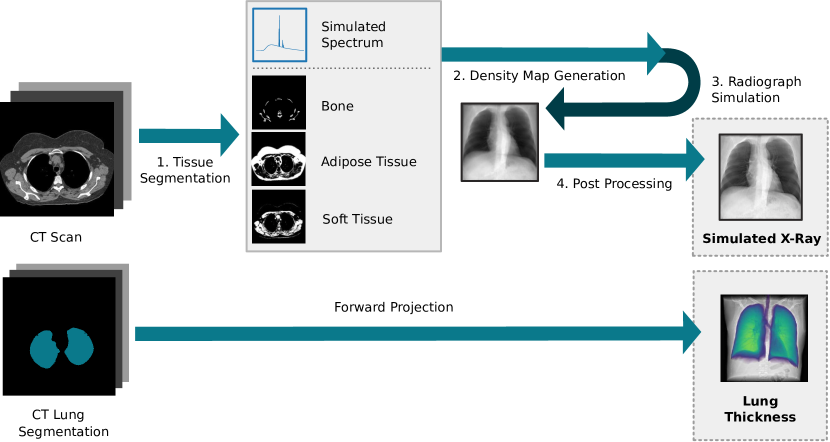
Figure 1: Illustrated workflow to obtain lung thickness maps and input radiographs for network training. A lung segmentation is performed on CTs. Next, the lung segmentation is forward projected and a 2D density map is retrieved. Then, the CT scan is split segmented into soft tissue, adipose tissue and bones in a first step. A spectrum is simulated for the desired kVp value and using the corresponding mass attenuation coefficients, a radiograph is simulated. The CT scan is then forward projected and post processed, to obtain the synthetic radiograph.

II.1 Dataset

Training data was retrieved from the Luna16 dataset [16], which consists of 888 CT scans. Only CT scans acquired with 120 kVp were used (N=656). Data was split into training (N=412), validation (N=113), and synthetic test set (N=131). For each CT scan 10 projections were obtained from different angles during the training and validation process, resulting in 4120 radiographs for training, 1130 radiographs for validation, and 1310 radiographs for the synthetic test set. Additionally, we use a second test set of 45 CT scans with corresponding real radiographs from our institute (Klinikum Rechts der Isar, Munich, Germany) in a retrospective study. Here, the timespan between CT and radiograph was below 6 months in order to avoid major morphological differences. Inclusion and exclusion data flow is illustrated in Fig. 2. The average age of the patients was 61.2 years, with 21 females and 24 males.

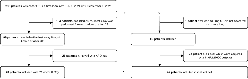
Figure 2: Flow chart showing inclusion and exclusion of patients. Out of 230 patients, 45 were eligible for the test set with real radiographs.

Data access was approved by the institutional ethics committee at Klinikum Rechts der Isar (Ethikvotum 87/18 S) and the data was anonymized. The ethics committee has waived the need for informed consent. All research was performed in accordance with relevant guidelines and regulations.

II.2 CT Data Preprocessing

In the preprocessing step, we perform two tasks: First, the CT scanner patient table is removed, as it does not appear in radiographs. To remove the patient table, for each slice in the CT volume, the slice image is converted into a binary mask by using a threshold, which divides the air from the body. Thin lines due to partial volume effects between the table and volume are removed by applying a opening filter. A connected components algorithm is applied to find the biggest connected object, which is the torso of the body. All other, smaller objects except the torso are removed from the slice. As a second task, the lung is segmented to retrieve the lung thickness later. Here we utilize an approach very similar to Sasidhar et al [17]. First, a binary mask of body tissue is generated. Air surrounded by body tissue is considered a lung-part and automatically extracted using a hole-filling algorithm. Next, the axial slice in the middle of the volume is inspected. The number of pixels on this slice is counted and all potential lung segments exceeding 1000 pixels are considered a lung part. The total 3D segmented volume composed of the real lung part in every slice is then considered as the lung volume. Using the final results of the CT preprocessing stage, we are now able to simulate radiographs with corresponding thicknesses for the training process.

II.3 X-Ray Spectrum Simulation

For the simulation of the radiographs and its post-processing, we set certain standard parameters of radiography imaging systems. The more accurately these parameters are determined and modeled, the more similar the simulated radiographs will look to the real radiographs. For our proof-of-concept study an accurate setting of known values (kVp) and a rough estimation of other values, which were more difficult to determine (scintillator material properties of the detector, detector thickness and post-processing parameters), was sufficient.

The x-ray spectrum is simulated using a semi-empirical model for x-ray transmission [18, 19, 20, 21]. To account for the detector material, the quantum efficiency $Q$ of the scintillator crystal with thickness $D_{\mathrm{scint}}$ and density $\rho_{\mathrm{scint}}$ is multiplied on the source spectrum:

$$Q=1-\exp(\mathrm{\mu}_{\mathrm{CsI}}(E)/\rho_{\mathrm{CsI}}\cdot D_{\mathrm{scint}}\cdot\rho_{\mathrm{scint}}),$$ (1)

where $\mathrm{\mu}_{\mathrm{CsI}}(E)/\rho_{\mathrm{CsI}}$ gives the mass attenuation coefficient for caesium iodid for a given energy E. The variables $\rho_{\mathrm{scint}}$ and $D_{\mathrm{scint}}$ represent the density and the thickness of the detector material. This yields the effective spectrum

$$\Phi(E)=\Phi^{\prime}(E)\cdot Q\cdot E,$$ (2)

which includes the aforementioned detector and x-ray tube effects, given the simulated spectrum $\Phi(E)^{\prime}$. The linear weighting with the energy $E$ considers the scintillation process.

In the simulation model, we used the detector values $\rho_{\mathrm{scint}}=4.51\mathrm{g}/\mathrm{cm}^{3}$ and $D_{\mathrm{scint}}=0.6mm$. To calculate the incidence spectrum on the detector, we assume the x-rays transmit a 3.5 mm aluminum target.

II.4 Material Segmentation

To attribute correct attenuation properties to the different tissue types in the human thorax, the CT scan is segmented into soft tissue, adipose tissue and bone volumes. The bone masks are generated by thresholding of HU values above 240, soft tissue masks are retrieved from HU values between 0 and 240, and adipose tissue voxels are extracted from values ranging from -200 to 0 HU. These values are in the ranges described by Buzug et al [22] and are slightly adapted to prevent overlapping or missing HU ranges.

For each material and each voxel we calculate the attenuation value for a certain energy, based on the descriptions for a model used for statistical iterative reconstruction [23]. In our simulation model, the attenuation values are calculated according to

$$\sum_{i=1}^{N}\rho^{\prime}\frac{\mu_{i}}{\rho_{i}}(E),$$ (3)

where $N$ is the total number of materials. The energy-dependency of the material $i$ is given by the mass attenuation coefficient $({\mu_{i}}/{\rho_{i}})(E)$ and $\rho^{\prime}$ labels its actual mass density.

As basis materials do not have the same density throughout the body (e.g. cortical and trabecular bone), it is of interest to introduce a relative scale factor: from the definition of the Hounsfield unit,

$$HU=\frac{\mu(E_{\mathrm{CT}})-\mu_{\text{Water}}(E_{\mathrm{CT}}))}{\mu_{\text{Water}}(E_{\mathrm{CT}})}\cdot 1000$$ (4)

and the definition of the linear attenuation coefficient

$$\mu(E_{\mathrm{CT}})=\frac{\mu}{\rho}(E_{\mathrm{CT}})\cdot\rho^{\prime}$$ (5)

we can solve for $\rho^{\prime}$:

$$\rho^{\prime}=\frac{\frac{HU}{1000}\cdot\mu_{\mathrm{Water}}(E_{\mathrm{CT}})+\mu_{\mathrm{Water}}(E_{\mathrm{CT}})}{\frac{\mu}{\rho}(E_{\mathrm{CT}})},$$ (6)

where $E_{\mathrm{CT}}$ does not depend on the simulated target X-ray spectrum, but rather the spectrum of the origin CT scanners. For 120 kVp CTs, we assume a mean energy $E_{\mathrm{CT}}$ of 70 keV.

This allows use to calculate the relative density $\rho_{i}^{\prime}$ for each voxel and for each material. These density volumes are forward projected using a cone-beam projector, as described in the next section, in order to obtain the projected density maps $d_{i}$ for each material $i$.

In our simulation model we account for the energy dependence of bone, adipose tissue and soft tissue. Hence the number of materials is three (N=3). Material information was retrieved from the NIST database [24] using the xraylib [25] framework. Tissue keys to retrieve mass attenuation coefficients from were ”Bone, Cortical (ICRP)”, ”Tissue, Soft (ICRP)” and ”Adipose Tissue (ICRP)”.

II.5 Forward Projection

To generate forward projections from the density volumes we utilized a cone-beam projector with a source-to-sample distance of 1680 mm and a sample-to-detector distance of 120 mm. We rotate the sample between $-10\deg$ and $10\deg$ and create 10 projections for each CT scan at 2$\deg$ steps. The detector size is set to 512 x 512 pixel. Beside the density volumes, we forward project the corresponding ground-truth lung segmentation for each CT scan. Therefore we retrieved projections $d_{i}$ of the density volumes and its corresponding 2-dimensional ground-truth lung-thickness map.

II.6 Radiograph Generation

From the projected thickness maps $d_{i}$ for each material we calculate the final intensity of each pixel in the radiograph according to:

$$I=\sum_{E=1}^{K}\Phi(E)\cdot\exp\left(\sum_{i}^{N}\rho^{\prime}\frac{\mu_{i}}{\rho_{i}}(E)\right)$$ (7)

given the energy dependent mass attenuation coefficient ${\mu_{i}(E)}/\rho_{i}$, the number of photons $\Phi(E)$ for a given energy $E$, a kilo-voltage peak $K$ and the number of basis materials $N$. Moreover, flat-field images are calculated using

$$F=\sum_{E=1}^{K}\Phi(E)$$ (8)

In a last step, the negative logarithmic normalized intensity is used to retrieve the radiograph in conventional clinical depiction (high transmission depicted as low signal),

$$I^{\prime}=-\log(I/F).$$ (9)

Using the described method, we are able to simulate the contrast between bone, adipose tissue and soft tissue for different kVp settings (Figure 3).

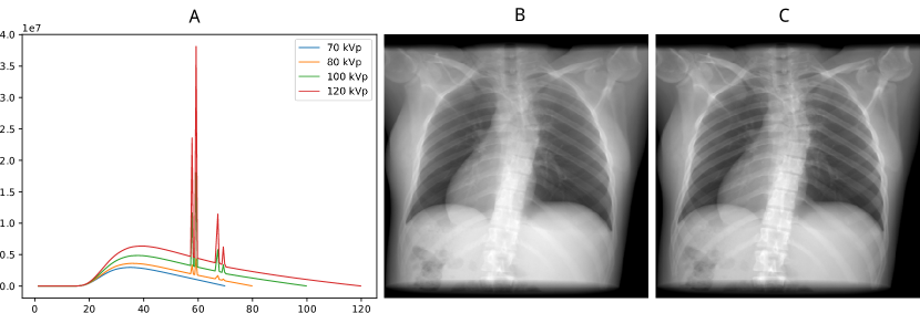
Figure 3: Simulated spectra for various kVp values (A). Synthetic 120 kVp radiograph with low bone-to-soft tissue contrast (B). Synthetic 70 kVp radiograph with stronger contrast between bones and soft tissue (C). Please note post-processing was not applied yet, which enhances contrast between bones and soft tissue further.

II.7 Postprocessing

X-ray imaging systems usually apply several postprocessing steps in order to increase the image quality. In our simulation model, two postprocessing steps are applied, namely a Look-up table (LUT) is used to alter the final intensities and a Laplacian pyramid processing is used to enhance high-frequencies in the radiograph. For that, 9 pyramids for a radiograph of 512 x 512 pixels are generated, whereby for each pyramid image $P_{i}$ a lower index i refers to a higher frequency pyramid. To reconstruct the image $P_{0}$ and $P_{1}$ frequencies are boosted by a factor of 2.0. Afterwards, a s-shaped LUT is applied similar to [26, 27]. For radiograph intensities, left clip is set at 0 and right clip at 8. Toe and shoulder parameters are set to a quadratic function to avoid hard cut-offs of the exposure scale.

II.8 CNN Architecture

For lung thickness estimation, we utilize a U-Net [8] architecture. The detailed architecture can be found in the supplementary material. As the output is an absolute value, it is important to use a linear activation function for the last layer. The loss function applied during training is of crucial importance for training the model and its ability to apply the model on real data later. A simple approach is the estimate of a groundtruth pixel $y_{i}$ and a predicted pixel $p_{i}$ to be calculated using a mean absolute error

$$\mathrm{MAE}=\frac{1}{N}\sum_{0}^{N}\mid y_{i}-p_{i}\mid$$ (10)

However, as the total lung volume estimate is of importance, we weight higher thicknesses more by multiplying the ground-truth thickness ($y_{i}$) on the loss function:

$$\mathrm{L}_{\mathrm{LUNG}}=\frac{1}{N}\sum_{i=0}^{N}\mid y_{i}-p_{i}\mid\cdot y_{i}\cdot w_{\mathrm{DEPTH}}$$ (11)

This will focus the network on lung structures only, as extrathoracic structures have a groundtruth-depth of 0. However, it requires the use of an additional lung segmentation network, as outside predictions are not penalized anymore. This is a desirable behaviour as the network later is not confused by a different patient pose in real radiographs (e.g. arms stretched down instead of up). As used by Alhashim et al [28] for image depth estimation, we further add a loss term for the derivative of the ground-truth:

$$\mathrm{L}_{\mathrm{GRAD}}=\sum_{i=0}^{N}\left(\mid\nabla_{x}(y_{i},p_{i})\mid+\mid\nabla_{y}(y_{i},p_{i})\mid\right)$$ (12)

In a last step, extrathoracic pixels are penalized

$$\mathrm{L}_{\mathrm{EXT}}=\frac{1}{N}\sum_{i=0}^{N}\mid y_{i}-p_{i}\mid\cdot\mathbf{I^{\star}}(y_{i})\cdot w_{\mathrm{EXT}}$$ (13)

with the indicator function $\mathbf{I^{\star}}$ returning 1 for thicknesses equal to zero:

$$\mathbf{I^{\star}}(x):=\left\{\begin{array}[]{ll}1&\text{if }x=0,\\ 0&\text{if }x>0.\end{array}\right.$$ (14)

The $w_{\mathrm{EXT}}=10$ assigns extra-thoracic thickness estimation errors the same weight as errors on 10mm deep lung tissue. Also $w_{\mathrm{DEPTH}}=2$ was empirically set. This results in the final loss function

$$\mathrm{L}=\mathrm{L}_{\mathrm{LUNG}}+\mathrm{L}_{\mathrm{GRAD}}+\mathrm{L}_{\mathrm{EXT}}$$ (15)

Previous work on lesion segmentation indicates a rather large tolerance for sensitivity parameters in a segmentation loss function [29]. CNN training was performed for 80 epochs. Learning rate was set to $10^{-4}$. Kernel initializers were set to the default value (glorot uniform initializer). The final model was selected from the epoch with the best validation loss.

II.9 Inference on Real Data

The model trained with simulated data can be applied on real radiographs. Due to the design of the loss function, there will be some extrathoracic pixels marked as lung pixels, which are removed by multiplying the prediction with a lung mask. To obtain the lung mask, we utilize a U-Net lung segmentation network trained with JSRT dataset [30] and JSRT mask data [31], similar to [32]. Small connected segmentation components (area smaller than 4100 pixels), which are usually extrathoracic segmentation predictions, were removed from the lung mask. The value 4100 was chosen empirically and is below the size of a lung lobe in the validation set. To maintain thickness estimations between the two lung lobes, the convex hull around the predicted lung mask segmentation is used to mask the thickness estimation.

II.10 PA Diameter Correction

As radiograph thickness was sometimes underestimated, we conducted an additional experiment to determine the thickness of outliers more accurately. While in the first experiment, the CNN directly yields the absolute thickness for each pixel, in this experiment, we only use the relative thickness distribution predicted by the CNN. The relative thickness is then multiplied with the lung diameter, which itself is derived from the measured patient diameter, in order to retrieve the absolute lung thickness.

For inference on the real test set, the posterior-anterior (PA) diameter $PA$ was determined from the CT scans in out experiments. The PA diameter can also be calculated on patients without a radiological modality (e.g. tape measure) on the approximated intersection between the first upper quarter and the second upper quarter of the lung.

Afterwards the CNN predicted thickness map of the radiograph is normalized: here, the maximum pixel value on the intersection line between the first upper third and the second upper third of the lung is obtained as a reference value. All thickness pixel values are then divided by this reference value. This yields a relative thickness value $R_{p}$ for each pixel.

To derive the lung diameter from the body diameter we introduce a correction factor $D^{\prime}$, which corresponds to the diameter of the lung divided by the patient’s diameter. This yields the absolute lung thickness $D_{p}$ for each pixel $p$ of the thickness map:

$$D_{p}=D^{\prime}\cdot R_{p}\cdot PA$$ (16)

The correction factor $D^{\prime}$ is set to 0.67 and was determined automatically from the mean of the diameters fractions of the first 50 CT scans in the training set: Here, for a CT scan, an axial slice in the upper third of the lung was chosen and the lung diameter on this slice was divided by the overall body diameter on this slice.

II.11 Implementation

The x-ray spectrum was simulated using SpekPy [19, 18, 20, 21], Machine learning models were implemented using Tensorflow [33] and Keras [34]. Cone-Beam forward projection was performed using the Astra toolbox [35]. Significance testing for correlation metrics was performed using Scipy (2019, Version 1.4.1).

III Results

Quantitative results of the total lung volume estimation are presented in table 1 for the synthetic test set and in table 2 for the real test set. Quantitative results on the synthetic test set were better than on the real test set: on the synthetic test set, the mean-absolute error was 0.19 liter with a positive correlation (r = 0.99). On the real test set, the mean-absolute error between the estimated lung volume and groundtruth volume was 0.75 liter with a positive correlation (r = 0.78. When accounting for the patient diameter, the error decreases to 0.69 liter with a positive correlation (r = 0.83). Hence, quantitative results on the synthetic test set were better than on the real test set. PA diameter correction did provide better results for the mean absolute error (MAE) and mean squared error (MSE) metrics than the prediction without correction.

	Without PA Corr.	With PA Corr.
MAE	0.75	0.69
MSE	0.91	0.78
Pearson	0.78	0.83
P-Value (Pearson)	$3.82\cdot 10^{-10}$	$1.98\cdot 10^{-12}$

Table 1: Quantitative results on real radiographs for enabled and disabled PA diameter correction.

	Without PA Corr.
MAE	0.19
MSE	0.05
Pearson	0.99
P-Value (Pearson)	$2.65\cdot 10^{-104}$

Table 2: Quantitative results on synthetic test set.

Qualitative results are shown in Fig. 4 for the synthetic test set and in Fig. 5 for the real test set. For the real test-set the thickness distribution between the groundtruth and the radiograph looks similar. However, higher thicknesses were underestimated for some cases. For the synthetic test set, we were additionally able to calculate the pixel-wise difference between thickness prediction and groundtruth. Here, higher differences tend to occur in thicker areas of the lung. Prediction and groundtruth lung volume of individual scans is further shown in a scatter plot (Figure 6) for both test sets. Here, for the synthetic test set, differences between groundtruth and prediction tend to be smaller than for the real test set.

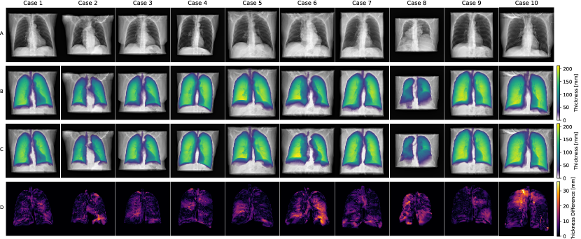
Figure 4: Qualitative results of various cases of the synthetic test set. Simulated input radiograph (A), predicted thickness (B), groundtruth thickness (C) and absolute difference between groundtruth and prediction (D) for various cases. The colorbar for B and C indicates lung thickness in mm. The colorbar for D indicates the per-pixel estimation error in mm.

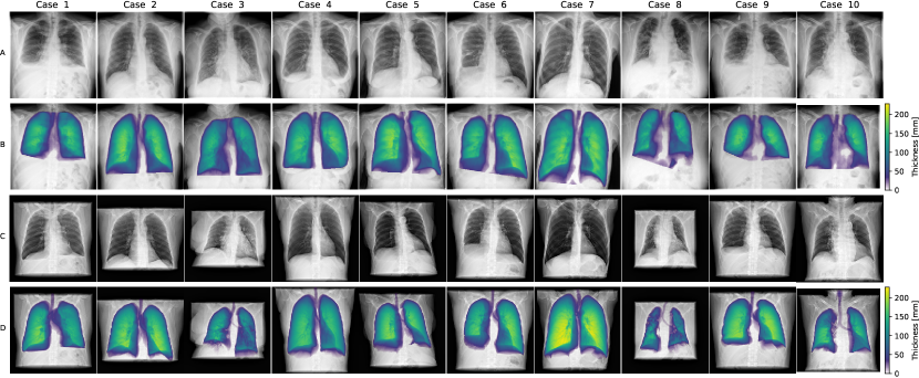
Figure 5: Qualitative results of various cases in the real test set with enabled PA diameter correction. Real input radiograph (A), predicted thickness using the real radiograph only (B), groundtruth radiograph synthesized from CT scans (C) and groundtruth thickness values derived from CT scans (D) for various cases, where each column represents one case. To compare the predicted thickness (B) of an input radiograph (A), the groundtruth CT scan and it’s lung segmentation was forward projected (C and D). Patient posture differences (e.g. arms up or down) between (A) and (C) are apparent. The colorbar indicates lung thickness in mm.

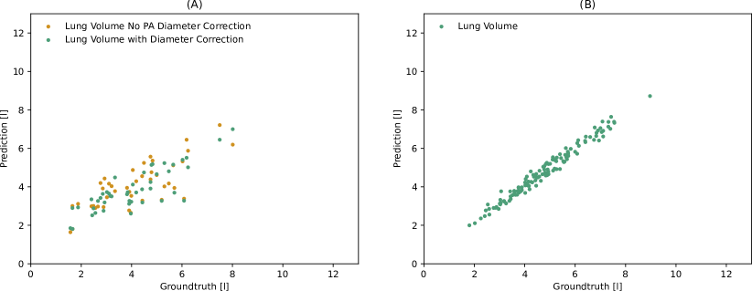
Figure 6: Prediction (y-axis) vs. groundtruth (x-axis) on the real test set (A) and the synthetic test set (B). On the real test, the PA diameter correction was optionally enabled.

IV Discussion

In this work we trained a model for per-pixel lung-volume estimation using synthetic radiographs and applied the trained model on real radiographs. Here, both quantitative and qualitative results obtained on synthetic and real radiographs were promising.

Transferring knowledge from CT scans to radiographs presents several hurdles: usually the pose in CT scans and radiographs is different. In CT, arms are positioned above the head, while in chest x-rays arms are positioned next to the body. We could effectively solve this problem by targeting the loss function on the lung area only and performing a lung segmentation, which was trained on real radiographs, afterwards.

One other obstacle in this project was the vendor specific post processing. These parts are typically closed source and not available from the vendors of the imaging platforms. Hence, it would be a great benefit if vendors would either provide the post-processing algorithm or supply a non-postprocessed version of the radiographs. Previously demonstrated methods that aim at training on synthetic data and application on real data, used histogram-equalization [13] to circumvent this problem as this usually results in a higher contrast between air and tissue and therefore makes the real data more adaptive to the synthetic data.

When looking at the results (Fig. 6), lungs with larger TLC values were underestimated a bit. We tried to solve this problem by multiplying the relative thickness with the lung PA diameter derived from the PA diameter of the patient. Here, overall results did improve with enabled PA diameter correction.

When comparing the results of the real test set with the synthetic test set, there is a clear difference in accuracy in predicting lung volume. In the real test set, a difference of 0.69 liter between groundtruth and prediction should not be underestimated, given the mean groundtruth volume of 4.07 liter. This difference may be due to multiple reasons: Beside morphological differences between simulated and real radiographs, such as the aforementioned post-processing routines, this may also be due to the different patient postures. Also, different inspiration levels in CT and CXR can play a role, as discussed in [6]. In addition, neglected physical effects such as Compton scattering could also account for differences between real radiographs and simulated radiographs. The results on the simulation data, however, strongly indicate that in case of a proper consideration of these physical effects a much lower lung volume prediction error can be achieved.

When comparing the results to Sogancioglu et al [6] our method shows a slightly higher error on the CT derived groundtruth (0.69 liter MAE vs. 0.59 liter MAE). However, our method offers one advantage: While still being able to infer the network on real X-Ray data, we train our network using only simulation data. This allows us to determine the lung thickness per pixel, while with Sogancioglu’s method, only a determination of the total volume of the lung is possible. Such thickness maps make it easier to understand the results of the prediction and provide additional applications for imaging techniques, as described in the introduction. Both methods could be combined in a way, where the normalized thickness map of our method is multiplied by the scalar prediction of their method.

Future work should investigate the additional use of lateral radiographs for training the thickness estimation network and try to improve the network architecture. Next, certain improvements could be made to the current model: For example, an U-Net based segmentation for the different tissue types instead of HU thresholding could be used. However, this would require a lot of additional annotation effort. Additionally, spectral CT data in the training set could also improve the quality of the segmentations used for material masks. Furthermore, future work could investigate the use of transferring knowledge from simulated radiographs to real radiographs to detect various pathologies or gain additional information for these pathologies.

V Acknowledgments

Funded by the Federal Ministry of Education and Research (BMBF) and the Free State of Bavaria under the Excellence Strategy of the Federal Government and the Länder, as well as by the Technical University of Munich – Institute for Advanced Study.

VI Author Contributions

F.P, D.P., L.B. and M.M. supervised the project. F.P, D.P. designed the research study. M.S. drafted the manuscript. P.S., M.S. and B.R extracted and preprocessed the data. M.S. and P.S. developed the deep learning models. M.S., T.S., K.M., K.T. developed the forward model to generate the simulated radiographs. M.S. analysed the results. R.S. implemented the post-processing algorithm. All authors reviewed the manuscript.

VII Model Availability

Inference models to test the model on own radiographs can be obtained from https://github.com/manumpy/lungthickness .

References

- [1] Paolo Biselli, Peter R. Grossman, Jason P. Kirkness, Susheel P. Patil, Philip L. Smith, Alan R. Schwartz, and Hartmut Schneider. The effect of increased lung volume in chronic obstructive pulmonary disease on upper airway obstruction during sleep. Journal of Applied Physiology, 119(3):266–271, 2015.
- [2] Alberto Hurtado, Walter W. Fray, Nolan L. Kaltreider, and William D. W. Brooks. Studies of Total Pulmonary Capacity and Its Subdivisions. V. Normal Values in Female Subjects. Journal of Clinical Investigation, 13(1):169–191, jan 1934.
- [3] J A Van Noord, J Clément, M Cauberghs, I Mertens, K P de Woestijne, and M Demedts. Total respiratory resistance and reactance in patients with diffuse interstitial lung disease. European Respiratory Journal, 2(9):846–852, 1989.
- [4] Yiying Huang, Cuiyan Tan, Jian Wu, Meizhu Chen, Zhenguo Wang, Liyun Luo, Xiaorong Zhou, Xinran Liu, Xiaoling Huang, Shican Yuan, Chaolin Chen, Fen Gao, Jin Huang, Hong Shan, and Jing Liu. Impact of coronavirus disease 2019 on pulmonary function in early convalescence phase. Respiratory Research, 21(1):163, dec 2020.
- [5] R. J. Pierce, D. J. Brown, M. Holmes, G. Cumming, and D. M. Denison. Estimation of lung volumes from chest radiogaphs using shape information. Thorax, 34(6):726–734, dec 1979.
- [6] Ecem Sogancioglu, Keelin Murphy, Ernst Th. Scholten, Luuk H. Boulogne, Mathias Prokop, and Bram van Ginneken. Automated Estimation of Total Lung Volume using Chest Radiographs and Deep Learning. may 2021.
- [7] Shadi Albarqouni, Javad Fotouhi, and Nassir Navab. X-ray in-depth decomposition: Revealing the latent structures. Lecture Notes in Computer Science (including subseries Lecture Notes in Artificial Intelligence and Lecture Notes in Bioinformatics), 10435 LNCS:444–452, 2017.
- [8] Olaf Ronneberger, Philipp Fischer, and Thomas Brox. U-Net: Convolutional Networks for Biomedical Image Segmentation. In Lecture Notes in Computer Science (including subseries Lecture Notes in Artificial Intelligence and Lecture Notes in Bioinformatics), volume 9351, pages 234–241. 2015.
- [9] A Andersen. Simultaneous Algebraic Reconstruction Technique (SART): A superior implementation of the ART algorithm. Ultrasonic Imaging, 6(1), jan 1984.
- [10] Yifan Wang, Zichun Zhong, and Jing Hua. DeepOrganNet: On-the-Fly Reconstruction and Visualization of 3D / 4D Lung Models from Single-View Projections by Deep Deformation Network. IEEE Transactions on Visualization and Computer Graphics, 26(1):960–970, 2020.
- [11] Fei Tong, Megumi Nakao, Shuqiong Wu, Mitsuhiro Nakamura, and Tetsuya Matsuda. X-ray2Shape: Reconstruction of 3D Liver Shape from a Single 2D Projection Image. In Proceedings of the Annual International Conference of the IEEE Engineering in Medicine and Biology Society, EMBS, volume 2020-July, pages 1608–1611. IEEE, jul 2020.
- [12] Franz Pfeiffer, Timm Weitkamp, Oliver Bunk, and Christian David. Phase retrieval and differential phase-contrast imaging with low-brilliance X-ray sources. Nature Physics, 2(4):258–261, 2006.
- [13] Hongchang Wang, Yogesh Kashyap, Biao Cai, and Kawal Sawhney. High energy X-ray phase and dark-field imaging using a random absorption mask. Scientific Reports, 6(1), nov 2016.
- [14] Marco Endrizzi and Alessandro Olivo. Absorption, refraction and scattering retrieval with an edge-illumination-based imaging setup. Journal of Physics D: Applied Physics, 47(50), dec 2014.
- [15] Konstantin Willer, Alexander A. Fingerle, Lukas B. Gromann, Fabio De Marco, Julia Herzen, Klaus Achterhold, Bernhard Gleich, Daniela Muenzel, Kai Scherer, Martin Renz, Bernhard Renger, Felix Kopp, Fabian Kriner, Florian Fischer, Christian Braun, Sigrid Auweter, Katharina Hellbach, Maximilian F. Reiser, Tobias Schroeter, Juergen Mohr, Andre Yaroshenko, Hanns Ingo Maack, Thomas Pralow, Hendrik Van Der Heijden, Roland Proksa, Thomas Koehler, Nataly Wieberneit, Karsten Rindt, Ernst J. Rummeny, Franz Pfeiffer, and Peter B. Noël. X-ray dark-field imaging of the human lung - A Feasibility study on a deceased body. PLoS ONE, 13(9), sep 2019.
- [16] Bram van Ginneken, Arnaud A. A. Setio, and Colin Jacobs. Luna 16 Dataset, Accessed 16 January 2020. Available on https://luna16.grand-challenge.org/data/, 2016.
- [17] B Sasidhar, Ramesh Babu D R, Ravi Shankar M, and Bhaskar Rao N. Automated Segmentation of Lung Regions using Morphological Operators in CT scan. International Journal of Scientific and Engineering Research, 4(9):1114–1118, 2013.
- [18] Robert Bujila, Artur Omar, and Gavin Poludniowski. A validation of SpekPy: A software toolkit for modelling X-ray tube spectra. Physica Medica, 75:44–54, jul 2020.
- [19] Artur Omar, Pedro Andreo, and Gavin Poludniowski. A model for the energy and angular distribution of x rays emitted from an x-ray tube Part I Bremsstrahlung production. Medical Physics, 47(10):4763–4774, oct 2020.
- [20] Artur Omar, Pedro Andreo, and Gavin Poludniowski. A model for the energy and angular distribution of x rays emitted from an x-ray tube Part II Validation of x-ray spectra from 20 to 300 kV. Medical Physics, 47(9):4005–4019, sep 2020.
- [21] Artur Omar, Pedro Andreo, and Gavin Poludniowski. A model for the emission of K and L x rays from an x-ray tube. Nuclear Instruments and Methods in Physics Research, Section B: Beam Interactions with Materials and Atoms, 437:36–47, dec 2018.
- [22] Thorsten Buzug. Computed tomography: From photon statistics to modern cone-beam CT. In Computed Tomography: From Photon Statistics to Modern Cone-Beam CT, page 477. Springer Berlin Heidelberg, 2008.
- [23] Korbinian Mechlem, Sebastian Ehn, Thorsten Sellerer, Eva Braig, Daniela Münzel, Franz Pfeiffer, and Peter B. Noël. Joint Statistical Iterative Material Image Reconstruction for Spectral Computed Tomography Using a Semi-Empirical Forward Model. IEEE Transactions on Medical Imaging, 37(1):68–80, 2018.
- [24] J H Hubbell and S M Seltzer. X-Ray Mass Attenuation Coefficients , Accessed 19 November, 2020. Available on https://www.nist.gov/pml/x-ray-mass-attenuation-coefficients, 2004.
- [25] Tom Schoonjans, Antonio Brunetti, Bruno Golosio, Manuel Sanchez Del Rio, Vicente Armando Solé, Claudio Ferrero, and Laszlo Vincze. The xraylib library for X-ray-matter interactions. Recent developments. Spectrochimica Acta - Part B Atomic Spectroscopy, 66(11-12):776–784, nov 2011.
- [26] Robert Andrew Davidson. Radiographic contrast-enhancement masks in digital radiography. PhD thesis, University of Sydney, 2006.
- [27] Lori L. Barski, Richard L. Van Metter, David H. Foos, Hsien-Che Lee, and Xiaohui Wang. New automatic tone-scale method for computed radiography. Proc. SPIE 3335, Medical Imaging 1998: Image Display, pages 164–178, jun 1998.
- [28] Ibraheem Alhashim and Peter Wonka. High Quality Monocular Depth Estimation via Transfer Learning. arXiv e-prints, abs/1812.1, 2018.
- [29] Tom Brosch, Youngjin Yoo, Lisa Y.W. Tang, David K.B. Li, Anthony Traboulsee, and Roger Tam. Medical Image Computing and Computer-Assisted Intervention - MICCAI 2015: 18th International Conference Munich, Germany, October 5-9, 2015 proceedings, part III. Lecture Notes in Computer Science (including subseries Lecture Notes in Artificial Intelligence and Lecture Notes in Bioinformatics), 9351:3–11, 2015.
- [30] Junji Shiraishi, Shigehiko Katsuragawa, Junpei Ikezoe, Tsuneo Matsumoto, Takeshi Kobayashi, Ken-ichi Komatsu, Mitate Matsui, Hiroshi Fujita, Yoshie Kodera, and Kunio Doi. Development of a Digital Image Database for Chest Radiographs With and Without a Lung Nodule. American Journal of Roentgenology, 174(1):71–74, jan 2000.
- [31] Bram van Ginneken, Mikkel B. Stegmann, and Marco Loog. Segmentation of anatomical structures in chest radiographs using supervised methods: a comparative study on a public database. Medical Image Analysis, 10(1):19–40, feb 2006.
- [32] Manuel Schultheiss, Sebastian A. Schober, Marie Lodde, Jannis Bodden, Juliane Aichele, Christina Müller-Leisse, Bernhard Renger, Franz Pfeiffer, and Daniela Pfeiffer. A robust convolutional neural network for lung nodule detection in the presence of foreign bodies. Scientific Reports, 10(1):12987, dec 2020.
- [33] Martín Abadi, Ashish Agarwal, Paul Barham, Eugene Brevdo, Zhifeng Chen, Craig Citro, Greg S. Corrado, Andy Davis, Jeffrey Dean, Matthieu Devin, Sanjay Ghemawat, Ian Goodfellow, Andrew Harp, Geoffrey Irving, Michael Isard, Yangqing Jia, Rafal Jozefowicz, Lukasz Kaiser, Manjunath Kudlur, Josh Levenberg, Dan Mane, Rajat Monga, Sherry Moore, Derek Murray, Chris Olah, Mike Schuster, Jonathon Shlens, Benoit Steiner, Ilya Sutskever, Kunal Talwar, Paul Tucker, Vincent Vanhoucke, Vijay Vasudevan, Fernanda Viegas, Oriol Vinyals, Pete Warden, Martin Wattenberg, Martin Wicke, Yuan Yu, and Xiaoqiang Zheng. TensorFlow: Large-Scale Machine Learning on Heterogeneous Distributed Systems, 2016.
- [34] François Chollet and Others. Keras, Accessed 7 December 2018. Available on https://github.com/fchollet/keras, 2015.
- [35] Wim van Aarle, Willem Jan Palenstijn, Jeroen Cant, Eline Janssens, Folkert Bleichrodt, Andrei Dabravolski, Jan De Beenhouwer, K. Joost Batenburg, and Jan Sijbers. Fast and flexible X-ray tomography using the ASTRA toolbox. Optics Express, 24(22):25129, oct 2016.