Quantitative absorption imaging of optically dense effective two-level systems

Abstract

Absorption imaging is a commonly adopted method to acquire, with high temporal resolution, spatial information on a partially transparent object. It relies on the interference between a probe beam and the coherent response of the object. In the low saturation regime, it is well described by a Beer Lambert attenuation. In this paper we theoretically derive the absorption of a $\sigma$ polarized laser probe by an ensemble of two-level systems in any saturation regime. We experimentally demonstrate that the absorption cross section in dense ⁸⁷Rb cold atom ensembles is reduced, with respect to the single particle response, by a factor proportional to the optical density $b$ of the medium. To explain this reduction, we developed a model that incorporates, in the single particle response, the incoherent electromagnetic background emitted by the surrounding ensemble. We show that it qualitatively reproduces the experimental results. Our calibration factor that has a universal dependence on optical density $b$ for $\sigma$ polarised light : $\alpha=1.17(9)+0.255(2)b$ allows to obtain quantitative and absolute, in situ, images of dense quantum systems.

I Introduction

Light propagation and attenuation in a dense medium are long lasting problems that have been particularly resistant to predictive models and experiments. The formal description of light propagation in a dilute medium was first reported by Bouguer Bouguer (1729) and later rediscovered by Lambert and Beer. The microscopic derivation of the Beer-Lambert law (BLL) relies on two premises: there should be no optical saturation nor the scatterers constituting the medium should influence each other. To get rid of the former constraint, the BLL can be easily modified and yields a decay of the light intensity following Lambert $W$ function Corless et al. (1996). This solution is exact in a dilute medium of two-level atoms and was used to develop absorption imaging technics and derivatives Pappa et al. (2011)

Including the full multi-level nature of an atomic system is straightforward under perfectly polarized probing, as it is only a matter of computing the effective dipole strength Gao (1993); Veyron et al. (2021). To modify minimally the BLL, Reinaudi et al. Reinaudi et al. (2007) originally proposed to reduce the saturation intensity with a single parameter $\alpha$, globally encapsulating any deviation from the idealized BLL. For the time being, $\alpha$ was used as a holdall that subsumes the undesired complexity arising from the presence of stray magnetic fields, imperfect probe polarization, multiple scattering or even the multilevel structure of the atomic system upon consideration. For the sake of atom number calibration, $\alpha$ has been estimated independently in numerous experiments Mordini et al. (2020); Yefsah et al. (2011); Reinaudi et al. (2007); Reinaudi (2008); Horikoshi et al. (2017); Seroka et al. (2019); Riedel et al. (2010); Kwon et al. (2012) with very disparate results even for similar probe conditions (see Tab. 1). There is no consensus ad idem concerning the acceptable values it should take nor regarding its scaling.

We recently demonstrated Veyron et al. (2021) by solving the multilevel Optical Bloch Equations in the single atom picture that stray magnetic fields or an imperfect probe polarization have little influence on $\alpha$, although an incoherent pumping dramatically increases its value.

Generalizing BBL to optically dense systems appears riskier at first glance, as it is required to use saturation parameters of the order of the optical thickness Reinhard et al. (2014). While a single atom response is exact and very well characterized experimentally in both unsaturated and saturated regimes Wrigge et al. (2007); Tey et al. (2009); Streed et al. (2012), the response of atomic clouds involves necessarily multiple scattering and high order correlations Lee et al. (2016), neither of them considered in the single atom model of BLL. Moreover, the geometry of the medium may favor -or hinder- a variety of many body responses under coherent illumination, as seen experimentally with endfire superradiance Inouye et al. (1999), or as predicted theoretically in the spectroscopy of 2D arrays of atoms Bettles et al. (2020).

It is now widely accepted that collective phenomena in dense media scale with powers of the optical thickness Labeyrie et al. (2004); Weiss et al. (2018) which is precisely the quantity that BLL endeavors to estimate. We expect in dense atomic media under resonant saturated illumination that scattered photons contribute to saturate incoherently albeit resonantly Pucci et al. (2017) the neighboring atoms in the forward and the backward directions. In this paper, we demonstrate experimentally that the value of $\alpha$ scales linearly with the optical density (OD). We propose a 1D model that accounts for collective effects via multiple scattering to explain this scaling.

$\alpha$	b0	Cloud type	Probe polarisation	Ref.
1.13(2)	0.5	BEC	Circular	Seroka et al. (2019)
1.11	1.2	BEC	Circular	Riedel et al. (2010)
2.0(2)	2.5	1D Li condensate	Circular	Horikoshi et al. (2017)
3.15(12)	5	1D BEC	Circular	Mordini et al. (2020)
2.12(1)	4.8	2D MOT	Linear	Reinaudi et al. (2007)
2.6(3)	-	Quasi 2D BEC	-	Yefsah (2011)
2.9	8.4	MOT	Linear	Reinaudi (2008)

Table 1: Review of the cross-section calibrations performed by different groups.

II Beer Lambert derivation in the saturating regime

In this section, we will derive the differential equation of propagation of a probe radiation (considered as a coherent field) in a continuous medium. The field at the point $\bm{r}$ is therefore obtained by summing the coherent incident field $\bm{E_{c}}(\bm{r})=\frac{E_{A}}{2}e^{ikz}\epsilon$ and the total scattered field obtained by the integral over space of the fields emitted by a continuous ensemble of dipoles Chomaz et al. (2012); Tey et al. (2009) :

$$\bm{E}(\bm{r^{\prime}})= \bm{E}(\bm{r})+\iiint_{V}n(\bm{r})\frac{3E_{A}}{2k}e^{ikz}i\frac{e^{ik|\bm{r^{\prime}}-\bm{r}|}}{|\bm{r^{\prime}}-\bm{r}|}\left(\bm{\epsilon}-\left(\bm{\epsilon}.\bm{u_{{rr^{\prime}}}}\right)\bm{u_{{rr^{\prime}}}}\right)d\bm{r}^{3}$$ (1)

where $\bm{u_{rr^{\prime}}}=(\bm{r^{\prime}}-\bm{r})/|\bm{r^{\prime}}-\bm{r}|$ is a vector unit, $n(\bm{r})$ is the atomic density and $V$ is the volume of integration. For an infinite homogeneous slab of atoms of width $dz$, the integration is carried for $x,y$ in $]-\infty,+\infty[$ and $z$ in $[z,z+dz]$.

In this expression, we consider only the dipole scattering in the far-field regime varying in $1/r$ which corresponds well to the regime of the data presented in section V ($nk^{-3}\ll 1$). We also emphasize that the above expression is only valid in the weak saturation approximation when a two-level system (TLS) is well approximated by a dipole. Performing the integration in cylindrical coordinates over a circle $R_{0}\gg 1/k$ (i.e. ignoring edge effects) for a constant atomic density in this disk $n(\bm{r})=n_{0}$ and a circular polarization, the first term proportional to $\bm{\epsilon}$ which is the on-axis scattering becomes $-n_{0}\frac{3E_{2}}{2k^{2}}e^{ik(z+dz)}2\pi\bm{\epsilon_{+}}dz$ and the second term depending on $\bm{u_{{rr^{\prime}}}}$ which is the off-axis scattering reads $n_{0}\frac{3E_{2}}{2k^{2}}e^{ik(z+dz)}\pi\bm{\epsilon_{+}}dz$. Eq. (1) can be simplified into:

$$\bm{E}(z+dz)= \bm{E}(z)\left(1-\frac{n_{0}}{2}\frac{6\pi}{k^{2}}e^{ikdz}dz\right)$$ (2)

which can be reformulated in a differential expression of the Beer-Lambert’s law in field :

$$\frac{d\bm{E}}{dz}= -\bm{E}\frac{n_{0}\sigma_{0}}{2}e^{ikdz}$$ (3)

where $\sigma_{0}=6\pi/k^{2}$ is the absorption cross section. For $kdz\ll 1$, Eq. (3) gives the traditional exponential attenuation of the intensity:

$$\frac{d|E|^{2}}{dz}= -|E|^{2}n_{0}\sigma_{0}$$ (4)

When the medium is saturated, the amplitude of the coherent field emitted on resonance by a single TLS is reduced but its radiation pattern for a given driving polarization is unchanged. The volume integral carried in Eq. (1) is still exact for an emitted dipole field reduced by a factor $1/(1+s_{c})$ where $s_{c}=\frac{2\Omega_{c}^{2}}{\Gamma^{2}}$ is the saturation parameter and $\Omega_{c}$ the Rabi frequency proportional to the incident electric field amplitude. This reduction factor of the coherently emitted field is directly related to the coherent scattering rate $\Gamma|\rho_{eg}|^{2}=\frac{\Gamma}{2}\frac{s_{c}}{(1+s_{c})^{2}}$ that can be derived from the Optical-Bloch equations of a TLS. To take into account the effect of saturation, the equation of propagation in field (Eq. (2) is modified into:

$$\bm{E}(z+dz)= \bm{E}(z)\left(1-\frac{1}{(1+s_{c})}\frac{n_{0}}{2}\frac{6\pi}{k^{2}}e^{ikdz}dz\right)$$ (5)

which gives the general form of the Beer-Lambert’s law for any saturation regime in intensity $I$:

$$\frac{dI(z)}{dz}\left(1+\frac{I(z)}{I_{\rm{sat}}}\right)= -n_{0}\sigma_{0}I(z)$$ (6)

where $I_{\rm{sat}}$ is the saturation intensity which is related to the cross section by $\sigma_{0}={\hbar\omega\Gamma}/({2I_{\rm{sat}}})$. For a multi-level system, it can be shown Veyron et al. (2021) that the coherent scattering rate is reduced and takes the form $\Gamma|\rho_{eg}|^{2}=\frac{\Gamma}{2}\frac{s_{c}}{(\alpha+s_{c})^{2}}$ where $\alpha$ depends on the probe polarization, residual magnetic field, detuning from the resonance or the ambient electromagnetic background. For ⁸⁷Rb, on resonance with the $|5S_{1/2},F=2\rangle$ to $|5P_{3/2},F=3\rangle$ cycling transition, a resonant probe with circular polarization has $\alpha=1$ (i.e. perfect two-level system) and $\alpha=1.829$ for linear polarization and $\alpha\in[1,1.829]$ for any other probe polarization. Including this correction, Eq. (6) becomes:

$$\frac{dI}{dz}\left(\alpha+\frac{I}{I_{\rm{sat}}}\right)= -n_{0}\sigma_{0}I$$ (7)

Eq. (7) can be analytically integrated over the propagation direction which leads to the expression of the optical density in the saturating regime:

$$b(x,y)=-\alpha\ln(T(x,y))+{s_{c}}(1-T(x,y))$$ (8)

where ${s_{c}}=I_{0}/I_{\rm{sat}}$ is the saturation parameter, $T(x,y)=\frac{I(x,y)}{I_{0}(x,y)}$ the probe transmission and $I_{0}(x,y)$ the incident imaging beam intensity.

Eq. (8) can also be written using the Lambert function $W$ as:

$$T(x,y)=\frac{\alpha}{{s_{c}}}W\left(\frac{{s_{c}}}{\alpha}e^{\frac{{s_{c}}-b(x,y)}{\alpha}}\right)$$ (9)

The optical density being an intrinsic cloud quantity, it should be independent of the probe beam properties. Following Reinaudi et al. (2007) the value of $\alpha$ in Eq. 8 can be determined by minimizing the influence of the saturation intensity of the probe on the measured optical density. In the following, we show that $\alpha$ actually depends on the optical density. We then propose a model that emphasizes the role of incoherent scattering from the ensemble.

III Experimental setup and data

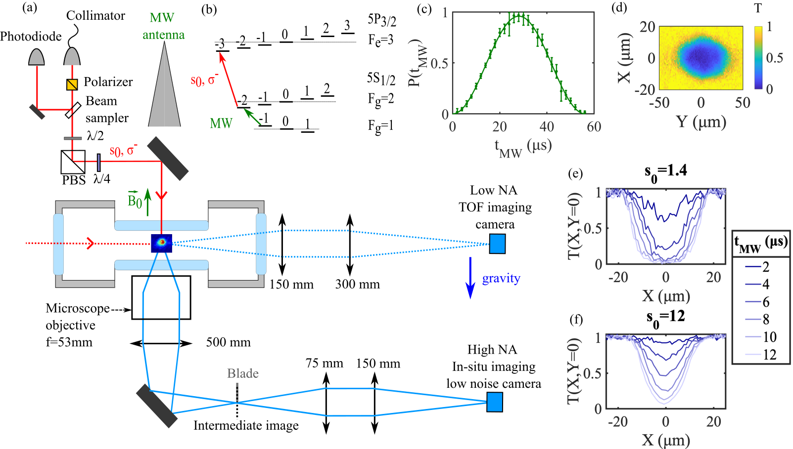
Figure 1: a) Experimental setup showing the two-imaging axis for TOF and in-situ absorption imaging. b) D2-line ⁸⁷Rb atomic structure. c) Rabi oscillation of the normalized atom number (points) between $\ket{F_{g}=1,m_{-1}}$ and $\ket{F_{g}=2,m_{-2}}$ as a function of the duration and a sinusoidal fit (solid line). The data are normalized with the optically repumped total atom number. d) 2D in-situ transmission image for $s_{0}=1.4$ and $t_{MW}=8$ µs. e)f) Cuts at $Y=0$ of the transmission for $s_{0}=1.3$ and $s_{0}=12$.

Thermal atoms in a pure $\ket{F_{g}=1,m_{F}=-1}$ spin state are prepared in a crossed dipole trap formed by two orthogonal and horizontal 1064 nm Gaussian beams. The dipole trap depths are $U_{x},U_{y}={33}(3),{11}(1)$ µK with respectively beam waists $w_{x},w_{y}=50(1),65(1)$ µm. The cloud has a temperature of $T=2.2(2)$ µK and a total atom number of $N_{tot}=1.92(15)\times 10^{5}$ which has been measured by absorption imaging of a $\pi$-polarized probe in the low saturation regime after long time-of-flight (TOF) that guarantee a peak OD lower than 0.5. The in-situ expected widths of this thermal cloud are $\sigma_{x},\sigma_{y}=\sqrt{k_{b}T/m\omega_{i}^{2}}=6.5(5),14.6(9)$ µm as calculated from the measured temperatures and trap frequencies ${\omega_{x},\omega_{y}}=\sqrt{4U/mw_{i}^{2}}=2\pi.{358(18),159(8)}$ Hz. The ambient magnetic field at the position of the atoms are characterized by MW spectroscopy and compensated. The residual field is below 10 mG. A constant offset of $B_{0}=512$ mG is then applied along the imaging beam propagation axis (i.e. gravity axis) and its direction matches a $\sigma_{-}$ configuration of the circularly polarized imaging probe.

From $\ket{F_{g}=1,m_{F}=-1}$ a control ratio of the total atom number are transferred to $\ket{F_{g}=2,m_{F}=-2}$ state by an on-resonance microwave pulse of duration $t_{MW}$. The transfer probability $P(t_{MW})=P_{tot}\sin^{2}(\pi t_{MW}/T_{MW})$ has a Rabi period $T_{MW}/2=28$ µs and an amplitude $P_{tot}=0.96$ (Fig. 1c). The peak atomic density is $2.1\times 10^{19}$ at/m³. For $t_{MW}=2$ µs, we can expect a central optical density of 1.1(1) for a circular polarized probe with scattering cross section $\sigma_{0}$.

After this transfer, the atoms in $\ket{F_{g}=2,m_{F}=-2}$ are imaged, in-situ, by absorption of a resonant circularly polarized imaging probe. The in-situ imaging system consists in a microscope objective (NA=0.44, $f_{eff}=53$ mm) followed by a 500 mm magnification lens that form an intermediate image. A secondary telescope magnifies this image by 2 on a low noise ($<3e^{-}$ rms read noise) Princeton CCD camera (16 µm pixel size). For each realization, three images are acquired corresponding to the probe absorption (first image $I_{\rm{at}}(x,y)$), probe profile (second image $I_{\rm{noat}}(x,y)$) and background (third without probe $I_{at}(x,y)$). To minimise the influence of air turbulences, the consecutive images are taken 400 µs apart. A circular aperture with a 3 mm diameter is installed in the Fourier plane of the secondary telescope. It reduces the effective NA of the objective to 0.185 and increases the depth of field to 22 µm, larger than the cloud width. The probe outcoupled from a single mode fiber has a measured waist of $w=1.13$ mm. Using the intermediate imaging plane, we measured a radial positioning offset to the beam center of 464 µm between the imaging probe Gaussian profile center and the center of the cloud leading to a reduction factor of the used intensity on the atoms by $0.71$ with respect to the probe center.

To make quantitative comparison between each experimental realization, the preparation of the cloud in $\ket{F_{g}=1,m_{F}=-1}$ is kept constant for all data sets. Only the MW duration ($t_{MW}=[2,4,6,8,10,12]$ µs) and probe saturation (${s_{c}}=[0.44,0.63,1.36,2.2,4.9,7.8,12.3,16.3,20.9,28,37.3,49]$) are varied. By adjusting the probe pulse duration from 12.9 µs to 3.7 µs, the number of scattered photons per atom is kept constant at $\approx 70$. In absence of atoms and taken into account the imaging system transmission (T=0.76), each pixel receives in between 200 and 6500 photons depending on the probe saturation. Each couple of parameters [$t_{MW},s_{0}$] is repeated 5 times for averaging.

To compensate for shot-to-shot fluctuations, the imaging pulses are all acquired by a calibrated photodiode from which the saturation intensity of each image are independently computed. We now analyze the local transmission of each cloud at the position $(x,y)$ as computed by $T=\left(I_{at}-I_{back}\right)/(I_{no,at}-I_{back})$.

IV Data

Following the spirit of Reinaudi et al. (2007), for each MW duration we use the transmission acquired for the various saturation intensity and compute, for every pixel $(x,y)$, the couple of parameter ${b(x,y),\alpha(x,y)}$ that make the OD calculated from Eq. (8) independent on the probe saturation. The resulting parameters are plotted in Fig. 2 where we can observe a clear correlation.

In the insets, we show 10 curves of $b$ vs. ${s_{c}}$ corresponding to $\alpha$ varying from 1 (black) to 11 (light grey). The best value of $\alpha$ minimizes std($b$). To reject the noise at very low transmission that is influenced by camera read noise and fluorescence we limit the analysis to transmissions T in the range $[0.05,+\infty[$. From the value of $\alpha$, the optical density is obtained by averaging it over all values of $s_{0}$. The upper inset corresponds to a pixel at the center of the cloud ($(b_{c},\alpha_{c})=(8.5,2.9)$) for $t_{MW}=6$ µs and the lower inset to a side shifted pixel ($(b_{s},\alpha_{s})=(8.3,3)$) with $t_{MW}=10$ µs. As the difference of position of the pixels compensates for the difference of central densities of the clouds, these two pixels correspond to a similar local optical density. Independently from their difference of position in the cloud, equivalent local optical densities lead to the same reduction of the scattering cross section. A linear fit of the entire dataset in Fig. 2 gives a slope of $0.255(2)$ an offset of $1.17(9)$ where the uncertainty is dominated by the uncertainty of the saturation parameter. This offset close to 1 shows that in the limit of low densities the atomic response is well modeled by an ensemble of independent TLS. The value of $\alpha$ at low atomic density depends both on the probe polarization and magnetic field direction but also linearly depends on the calibration of the saturation intensity as observed by the atomic cloud. The calibration of the offset between probe center and atoms was important in this respect. The dependance of $\alpha$ on $b$ shows that $\alpha$ is not solely determined by the probe properties but also depends on the optical density which is a signature of the influence of multiple scattering.

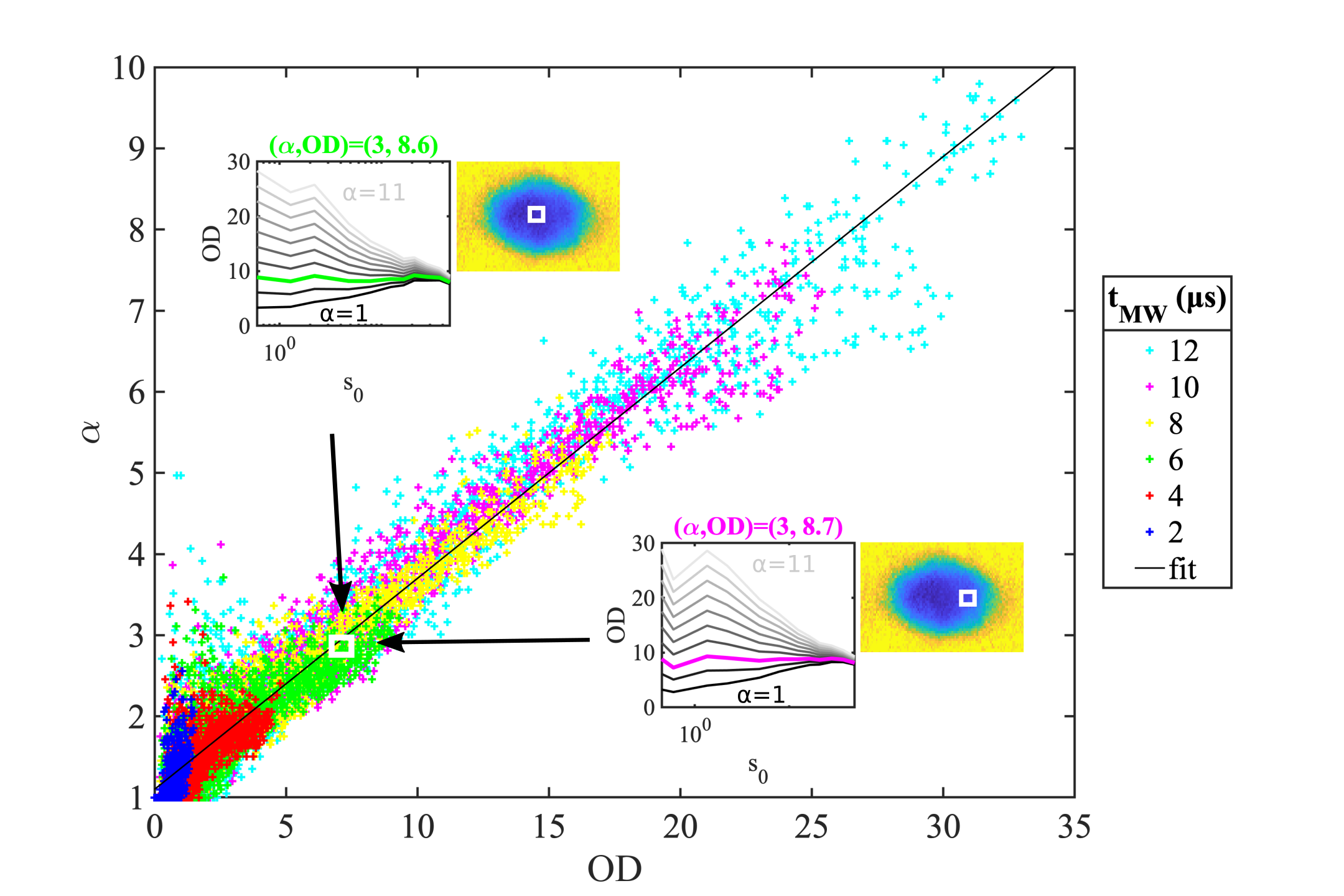
Figure 2: Correction factor $\alpha$ vs. the optical density for all MW datasets ($2,4,6,8,10,12$ µs). Each point corresponds to 1 pixel and the solid line is a linear fit to the data $\alpha=1.17(9)+0.255(2)b$.

V Model

As shown in Veyron et al. (2021), the coherent scattering properties of a TLS probed by circularly polarized light are almost insensitive at first order to experimental imperfections such as magnetic bias orientation or incident polarization. Nevertheless, in the same paper, it was shown that the presence of an incoherent electromagnetic background will influence the coherent response of atoms. Here, we show that such incoherent background could arise from multiple scattering in the medium and we propose a model of propagation that can be quantitatively compared to the data. In the model, we consider the propagation of the coherent probe in a cloud that is homogeneous in the transverse directions and has Gaussian density profile in the propagation direction. The system is translation invariant in the transverse plane $(x,y)$. The electromagnetic field and intensity therefore only depend on $z$. For a resonant $\sigma$ polarized probe, the scattering properties of an atom embedded in an incoherent electromagnetic background are well described Veyron et al. (2021) by an effective TLS. Its coherent and total scattering rates, as deduced from the density matrix calculation, are given by :

$$R^{(coh)}_{sca}= \frac{\Gamma}{2\alpha}\frac{{\frac{s_{c}}{\alpha}}}{\left(1+\frac{s_{c}}{\alpha}\right)^{2}}$$ (10)

$$R^{(tot)}_{sca}= \frac{\Gamma}{2}\left(\frac{\frac{s_{c}}{\alpha}}{1+\frac{s_{c}}{\alpha}}+\frac{\frac{s_{i}}{\alpha_{c}}}{1+\frac{s_{i}}{\alpha_{c}}}\right)$$

where the corrected scattering rates are $\alpha=\alpha_{\rm{SA}}\left(1+s_{i}\right)$ and $\alpha_{c}=1+s_{c}$, where $\alpha_{SA}$ is the single atom reduction of the cross section that depends on polarization, detuning and offset field. In this work, we have $\alpha_{SA}=1$ corresponding to on resonance $\sigma$ polarization.

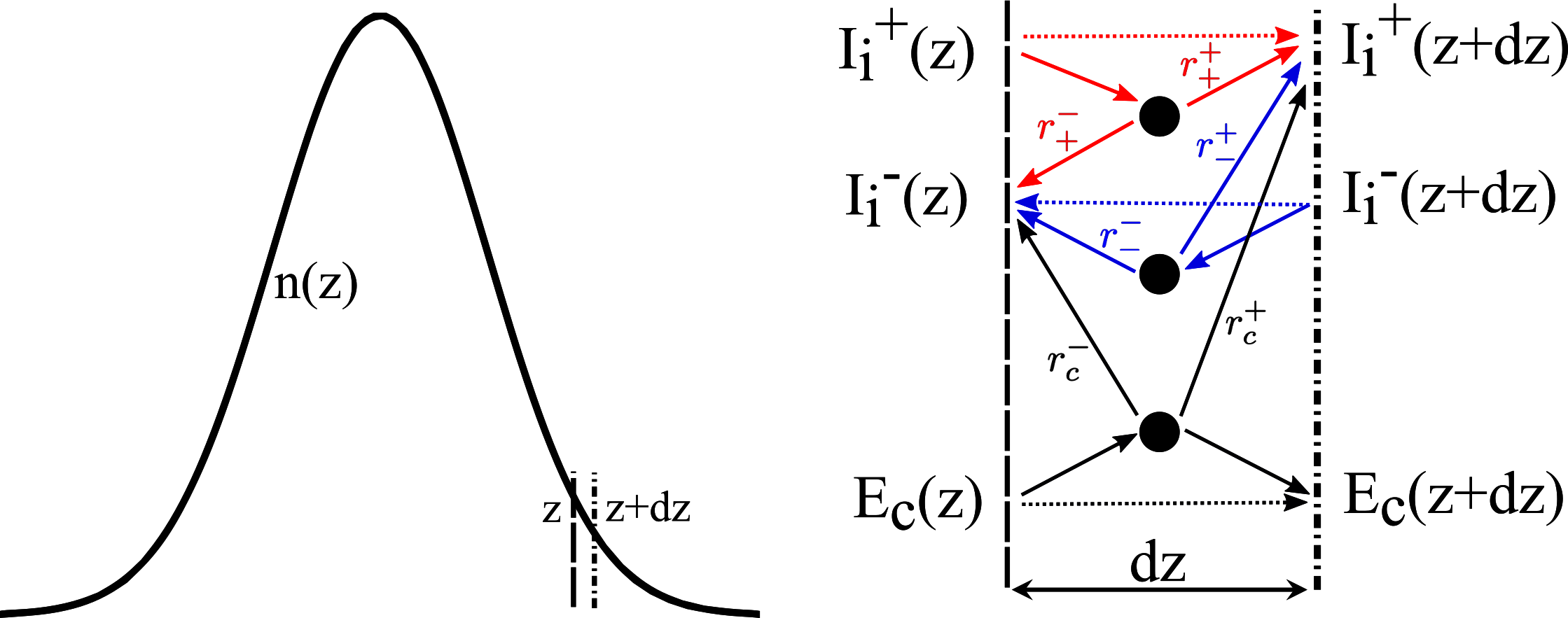
Figure 3: 1D model for the coherent and incoherent propagation and conversion of light between adjacent layers. The coherent and incoherent scattering rates are given by eq. 10. The spatial repartition are taken as $r_{+}^{+}=1-r_{+}^{-}=r_{-}^{-}=1-r_{-}^{+}=r_{c}^{+}=1-r_{c}^{-}=1/2$ (see text).

To numerically solve our model, we divide the propagation direction in infinitely small slabs of width $dz$. For each slab, we derive from the scattering rate expressions (Eq. LABEL:) a set of differential equations that relates the intensity profile of the coherent intensity $I_{c}(z)$, forward incoherent intensity $I_{i}^{+}(z)$ and backward incoherent intensity $I_{i}^{-}(z)$. The set of equation are expressed in terms of the nondimensionalized saturation intensity parameters $s_{c}(z)=I_{c}(z)/I_{\rm{sat}}$, $s_{i}^{+}(z)=I_{i}^{+}(z)/I_{\rm{sat}}^{\rm{iso}}$, $s_{i}^{-}(z)=I_{i}^{-}(z)/I_{\rm{sat}}^{\rm{iso}}$ where $I_{\rm{sat}}^{\rm{iso}}=\alpha^{\rm{iso}}I_{\rm{sat}}=2.12I_{\rm{sat}}$.

$$\frac{ds_{c}}{dz}= -n(z)\sigma_{0}\frac{s_{c}}{1+s_{c}+s_{i}}$$ (11)

$$\frac{ds_{i}^{(+)}}{dz}= -\frac{n(z)\sigma_{0}^{\rm{iso}}}{2}\left(\frac{s_{i}^{(+)}-s_{i}^{(-)}}{1+s_{c}+s_{i}}-\frac{s_{c}(s_{c}+s_{i})}{\left(1+s_{c}+s_{i}\right)^{2}}-\frac{s_{c}}{\left(1+s_{c}+s_{i}\right)^{2}}\right)$$

$$\frac{ds_{i}^{(-)}}{dz}= -\frac{n(z)\sigma_{0}^{\rm{iso}}}{2}\left(\frac{s_{i}^{(-)}-s_{i}^{(+)}}{1+s_{c}+s_{i}}-\frac{s_{c}(s_{c}+s_{i})}{\left(1+s_{c}+s_{i}\right)^{2}}-\frac{s_{c}}{\left(1+s_{c}+s_{i}\right)^{2}}\right)$$

where the isotropic cross section is $\sigma_{0}^{\rm{iso}}={\hbar\omega\Gamma}/({2I_{\rm{sat}}^{\rm{iso}}})$ and the total incoherent intensity is $s_{i}=s_{i}^{(+)}+s_{i}^{(-)}$. The prefactor $1/2$ corresponding to $r_{c/+/-}^{+/-}$ in Fig. 3 accounts for equally distributed of backward and forward scattered intensities. In the derivatives of $s_{i}^{\pm}$ in Eq. (11), the first term account for re-scattering of incoherent field which is isotrope ($r_{+}^{+}=r_{+}^{-}$ and $r_{-}^{-}=r_{-}^{+}$), the second one accounts for the temporally incoherent ($ti$) scattering of the coherent field (i.e. resonant fluorescence) which is also isotropic ($r_{c}^{-,ti}=r_{c}^{+,ti}$). The last term that conserves energy corresponds to the coherent field scattering in a temporally coherent but spatially incoherent ($si$) field arising from the discrete random position of atoms in an ensemble that we assume to be isotropic ($r_{c}^{-,si}=r_{c}^{+,si}$). This spatially incoherent field is out-of-phase with the coherent probe and its effect on the coherence term of the density matrix $\rho_{eg}$ will spatially average to 0. As checked numerically, for large saturation, the scattering being mostly temporally incoherent, this assumption has very little consequence on the results. In this model both temporally and spatially incoherent contributions are summed in the incoherent intensity : $r_{c}^{+/-}=r_{c}^{+/-,ti}+r_{c}^{+/-,si}$.

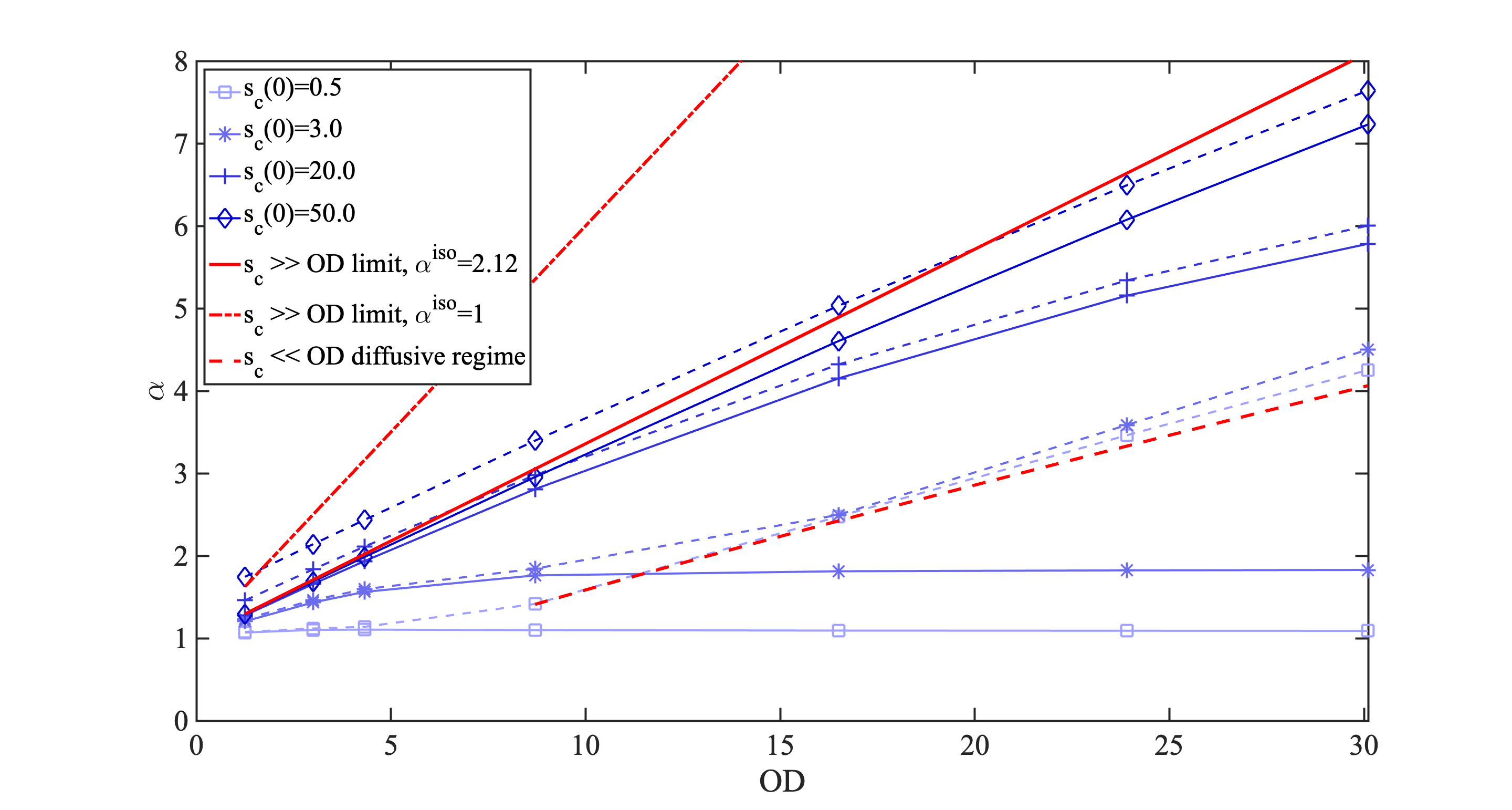
Figure 4: $\alpha$ parameters calculated from the saturated scattering model (Eq. 11). The simulated probe saturation intensities are comparable to the experiment : $s_{c}=0.5$ in light blue (bottom) to $s_{c}=50$ in dark blue (top). The line (resp. dashed line) correspond to the value of $\alpha$ as calculated from the sole coherent transmission $T_{c}=s_{c}(L)/s_{c}(0)$ (resp. the total transmission $T=(s_{c}(L)+\alpha^{\rm{iso}}s_{i}^{+}(L)\Omega/(2\pi))/s_{c}(0)$, where $\alpha^{\rm{iso}}s_{i}^{+}(L)\Omega$ is the fluorescence background emitted in the solid angle $\Omega$ of the imaging system). In red, the analytical large saturation limit for (plain line) an effective TLS approximation of a MLS with $\sigma_{0}^{\rm{iso}}=\sigma_{0}/\alpha^{\rm{iso}}$, (dot-dashed line) an ideal scalar TLS corresponding to $\sigma_{0}^{\rm{iso}}=\sigma_{0}$ and (dashed) the diffusive regime (see text).

The value of $\alpha$ for different probe intensities are presented in Fig. 4 as a function of the integrated optical density. For small probe saturation, the conversion of the coherent probe field into incoherent intensity ($s_{i}$) cannot generate high incoherent intensity ($s_{i}\ll 1$) and should therefore not affect the value of $\alpha$ in the coherent propagation (Eq. (11)). Nevertheless, for high optical density, we are in the diffusive regime. Along the propagation, while the coherent field is exponentially reduced in the mean free path length $l_{sc}=1/(n\sigma_{0})$ and quickly disappears, the incoherent field, that will also be detected on the camera, is only algebraically reduced $T_{diff}\propto 1/b=C/b$ Garcia et al. (1992); Guerin et al. (2017). In this regime, it is the dominating contribution that scales as $\alpha\approx b/\ln(2\pi b/C\Omega)$ where $\Omega$ is the solid angle of the imaging system (dashed red asymptote in Fig. 4 with $C=1$). Here ($b\gg s_{c}$), the increase of $\alpha$ does not correspond to a reduction of the absorption cross section but rather to an excess of detected light. In the opposite high saturation regime ($s_{c}\gg b$), the probe intensity is little depleted, and the incoherent saturation intensity becomes homogeneous along the propagation. By energy conservation we have $s_{i}={s_{c}}(1-T)/(2\alpha^{\rm{iso}})$. For high saturation, the last term in eq. 8 dominates in the expression of the optical density $b\approx s_{0}(1-T)$. It leads to an expected reduction of the coherent absorption cross section that scales as $\alpha=1+s_{i}\approx 1+b/(2\alpha^{\rm{iso}})$ (red curve in Fig. 4). Fig. 4 shows the expected value of $\alpha$ for a scalar TLS model where both coherent and incoherent scattering are considered $\sigma$ polarized ($\alpha^{\rm{iso}}=1$). We observe that it over-evaluates $\alpha$ while an effective TLS with isotropic incoherent scattering $\alpha^{\rm{iso}}=2.12$ has a slope 1/(2*2.12)=0.24 in good correspondence with the experimentally measured one (0.26). Given that the experimental value of $\alpha$ is averaged over all $s_{c}$ for a given $b$ and that this model does not take into account the transverse inhomogeneity of the cloud or the Mollow spectrum of the incoherently scattered light, the so close correspondence of the slopes is certainly fortuitous. We nevertheless believe that this model captures most of the physical origin for the increase of $\alpha$ with $b$.

VI Conclusions

In conclusion we have shown that the reduction of the apparent absorption cross section is connected, in the diffusive regime ($b\gg s_{c}$), to the residual diffuse transmission and, in the saturating regime, to the ambient electromagnetic background originating from multiple incoherent scattering in the cloud ($s_{i}$). In both cases, this correction is shown to scale mainly linearly with the optical density and reproduces well the experimentally observed dependance of $\alpha$. In contrast with previously proposed calibration methods Reinaudi et al. (2007) that are commonly used in the community, this study shows that the reduction of cross section is not unique for an entire cloud. For a circular probe polarization under well controlled magnetic field orientation and laser detuning, the correction factor : $\alpha=1.17(9)+0.255(2)b$ seems universal and independent of the position in the cloud. The offset $\alpha_{0}=1.17(9)$ ultimately depends on a fine calibration of the saturation parameter and should be equal to 1 for a perfectly calibrated $\sigma$ light. A similar calibration could certainly be performed for other typical configuration such as linear $\pi$ probes. A strength of the proposed model is to take into account both the saturated response of a single atom embedded in an electromagnetic environment and the collective participation of the surrounding atoms to this environment in a self-consistent solution. At the cost of numerical computation power, the proposed 1D model could certainly be extended to 3D and incorporate modifications on the reabsorption cross section.

References

- Bouguer (1729) P. Bouguer, Paris, France: Claude Jombert (1729).
- Corless et al. (1996) R. M. Corless, G. H. Gonnet, D. E. G. Hare, D. J. Jeffrey, and D. E. Knuth, Adv. Comput. Math. 5, 329 (1996).
- Pappa et al. (2011) M. Pappa, P. C. Condylis, G. O. Konstantinidis, V. Bolpasi, A. Lazoudis, O. Morizot, D. Sahagun, M. Baker, and W. von Klitzing, New J. Phys. 13, 115012 (2011).
- Gao (1993) B. Gao, Phys. Rev. A 48, 2443 (1993).
- Veyron et al. (2021) R. Veyron, V. Mancois, J.-B. Gerent, G. Baclet, P. Bouyer, and S. Bernon, (2021), arXiv:2110.08894 [physics.atom-ph] .
- Reinaudi et al. (2007) G. Reinaudi, T. Lahaye, Z. Wang, and D. Guéry-Odelin, Opt. Lett. 32, 3143 (2007).
- Mordini et al. (2020) C. Mordini, D. Trypogeorgos, A. Farolfi, L. Wolswijk, S. Stringari, G. Lamporesi, and G. Ferrari, Phys. Rev. Lett. 125, 150404 (2020).
- Yefsah et al. (2011) T. Yefsah, R. Desbuquois, L. Chomaz, K. J. Günter, and J. Dalibard, Phys. Rev. Lett. 107, 130401 (2011).
- Reinaudi (2008) G. Reinaudi, Theses, Université Pierre et Marie Curie - Paris VI (2008).
- Horikoshi et al. (2017) M. Horikoshi, A. Ito, T. Ikemachi, Y. Aratake, M. Kuwata-Gonokami, and M. Koashi, J. Phys. Soc. Jpn. 86, 104301 (2017).
- Seroka et al. (2019) E. M. Seroka, A. V. Curiel, D. Trypogeorgos, N. Lundblad, and I. B. Spielman, Opt. Express 27, 36611 (2019).
- Riedel et al. (2010) M. F. Riedel, P. Böhi, Y. Li, T. W. Hänsch, A. Sinatra, and P. Treutlein, Nature 464, 1170 (2010).
- Kwon et al. (2012) W. J. Kwon, J. yoon Choi, and Y. il Shin, J. Korean Phys. Soc. 61, 1970 (2012).
- Reinhard et al. (2014) A. Reinhard, J.-F. Riou, L. A. Zundel, and D. S. Weiss, Optics Communications 324, 30 (2014).
- Wrigge et al. (2007) G. Wrigge, I. Gerhardt, J. Hwang, G. Zumofen, and V. Sandoghdar, Nature Phys. 4, 60 (2007).
- Tey et al. (2009) M. K. Tey, G. Maslennikov, T. C. H. Liew, S. A. Aljunid, F. Huber, B. Chng, Z. Chen, V. Scarani, and C. Kurtsiefer, New J. Phys. 11, 043011 (2009).
- Streed et al. (2012) E. W. Streed, A. Jechow, B. G. Norton, and D. Kielpinski, Nat Commun 3, 933 (2012).
- Lee et al. (2016) M. D. Lee, S. D. Jenkins, and J. Ruostekoski, Phys. Rev. A 93, 063803 (2016).
- Inouye et al. (1999) S. Inouye, A. P. Chikkatur, D. M. Stamper-Kurn, J. Stenger, D. E. Pritchard, and W. Ketterle, Science 285, 571 (1999).
- Bettles et al. (2020) R. J. Bettles, M. D. Lee, S. A. Gardiner, and J. Ruostekoski, Commun Phys 3, 141 (2020).
- Labeyrie et al. (2004) G. Labeyrie, D. Delande, C. Müller, C. Miniatura, and R. Kaiser, Optics Communications 243, 157 (2004).
- Weiss et al. (2018) P. Weiss, M. O. Araújo, R. Kaiser, and W. Guerin, New J. Phys. 20, 063024 (2018).
- Pucci et al. (2017) L. Pucci, A. Roy, T. S. do Espirito Santo, R. Kaiser, M. Kastner, and R. Bachelard, Phys. Rev. A 95, 053625 (2017).
- Yefsah (2011) T. Yefsah, Theses, Université Pierre et Marie Curie - Paris VI (2011).
- Chomaz et al. (2012) L. Chomaz, L. Corman, T. Yefsah, R. Desbuquois, and J. Dalibard, New J. Phys. 14, 055001 (2012).
- Garcia et al. (1992) N. Garcia, A. Z. Genack, and A. A. Lisyansky, Phys. Rev. B 46, 14475 (1992).
- Guerin et al. (2017) W. Guerin, M. Rouabah, and R. Kaiser, J. Mod. Opt. 64, 895 (2017).