EgoNN: Egocentric Neural Network for Point Cloud Based 6DoF Relocalization at the City Scale*

Abstract

The paper presents a deep neural network-based method for global and local descriptors extraction from a point cloud acquired by a rotating 3D LiDAR. The descriptors can be used for two-stage 6DoF relocalization. First, a course position is retrieved by finding candidates with the closest global descriptor in the database of geo-tagged point clouds. Then, the 6DoF pose between a query point cloud and a database point cloud is estimated by matching local descriptors and using a robust estimator such as RANSAC. Our method has a simple, fully convolutional architecture based on a sparse voxelized representation. It can efficiently extract a global descriptor and a set of keypoints with local descriptors from large point clouds with tens of thousand points. Our code and pretrained models are publicly available on the project website. 

I Introduction

Relocalization at a city-scale is an emerging task with various applications in robotics and autonomous vehicles, such as loop closure in SLAM or kidnapped robot problem [1]. A typical approach is a two-step process: 1) coarse localization using global descriptors, 2) precise 6DoF pose estimation by pairwise registration.

The development of LiDAR technologies enabled the shift from an image-based approaches, affected by scene appearance changes, to 3D methods relying on the scene geometry. Several learning-based methods for LiDAR-based global descriptor extraction were recently proposed [2, 3, 4], but they are intended for relatively small point clouds with few thousand points. In contrast, scans from modern 3D LiDARs, such as Velodyne HDL-64E, show 360^∘ view of the scene and contain tens of thousand points. For computational efficiency, methods operating on such large point clouds typically convert them to some form of intermediate representation, such as a set of multi-layer 2D images [5], before further processing. This hides some information about a scene structure and can adversely impact the performance.

In this work, we address the problem of a point cloud-based relocalization at a city scale. We consider a typical scenario [3], where the map consists of LiDAR scans with known 6DoF absolute pose, and the aim is to find a 6DoF pose of a query scan. We propose a network architecture to efficiently extract both a global descriptor for coarse-level place recognition and a set of keypoints with their local descriptors for 6DoF pose estimation. The network is designed to efficiently process large point clouds, with tens of thousand points, acquired by modern rotating LiDAR sensors. A similar approach is proposed in [3], but their DH3D method handles smaller point clouds with less than 10k points. The design of our method is inspired by the state-of-the-art MinkLoc3D [4] global point cloud descriptor. It processes raw 3D point clouds using a sparse voxelized representation and 3D convolutional architecture without the need for a point cloud conversion to an intermediate form. However, MinkLoc3D is intended for smaller point clouds with few thousand points. In this work, we investigate the scalability of this architecture to much larger point clouds.

The main contribution of our work is the development of an efficient network architecture for extraction of both a global descriptor for coarse-level place recognition and a set of keypoints with their local descriptors for a precise 6DoF pose estimation. The method efficiently processes raw point clouds acquired by modern 360^∘ rotating LiDAR sensors, with tens of thousand points. Additionally, we make our code, pre-trained models, and training/evaluation splits publicly available. We believe this will help advance state of the art by allowing the community to evaluate future methods against the same baselines.

II Related work

Early methods to generate a global point cloud descriptor use handcrafted features. Most of the approaches [6, 7, 8, 9] use statistical calculations and histogram aggregations to describe a scene. ScanContext [10] represents a scene as a bird’s-eye-view RGB image that describes geometrical information of an egocentric environment. Seed [11] extends this idea by first segmenting a point cloud, and Weighted ScanContext [12] uses the intensity information of points to enhance geometric features. LiDAR Iris [13] introduces a binary signature image computed from a bird’s-eye-view point cloud representation.

The alternative group of methods leverages deep neural networks to produce a discriminative global descriptor in a learned manner. Most of them operates on relatively small point clouds built by accumulating consecutive 2D LiDAR scans during the vehicle traversal and downsampling the merged cloud. For instance, PointNetVLAD [2], one of the first learned global descriptors, operates on point clouds spanning 20 m in the longitudinal direction and downsampled to 4096 points. Several methods [14, 3, 4] improve upon NetVLAD, but all of them are operate on point clouds with the same characteristic. They poorly scale to larger clouds, with tens of thousands points and covering the area with over 100 m radius, acquired using modern 3D rotating LiDARs.

For computational efficiency, methods operating on larger scans usually convert them to an intermediary representation before processing with a deep neural network. OREOS [15] projects the input into a 2D range image using a spherical projection model. OverlapNet [1] extracts four different 2D representations: range, intensity values, normals, and semantic classes. DiSCO [5] converts a point cloud into a set of multi-layer 2D images in cylindrical coordinates. Such conversion loses some information about the scene structure, which may adversely impact the performance. Our method operates on raw point clouds from a modern 3D LiDAR, without the need for an intermediary representation.

In addition to a global descriptor extraction, some recent methods produce additional information that can be used for an initial alignment of two point clouds before the final registration using an ICP [16] or similar method. OREOS [15] and DiSCO [5] estimate a relative yaw angle between two scans. In addition to yaw angle, OverlapNet [1] estimates an overlap between two point clouds. Our method regresses a set of keypoints with their descriptors that can be used to directly estimate relative 6DoF pose without the need for an initial alignment.

The closest approach to ours is DH3D [3], which is the first method that unifies global descriptor extraction with local features computation. However, DH3D is handles relatively small point clouds with 8k points and spanning a 20 m distance in the longitudinal direction. Our method scales to much larger clouds with tens of thousand points.

Some recent deep learning-based point cloud registration methods [17, 18] directly estimate relative 6DoF pose between two point clouds without finding correspondences between local features. However, results in [19] suggest that direct keypoint correspondence estimation can more accurately register two partially overlapping point clouds and better handle larger initial misalignment. Hence our method computes repetitive keypoints and discriminative local descriptors that can be used for a robust RANSAC-based 6DoF pose estimation.

III EgoNN: Egocentric neural network for global and local descriptors

We propose a neural network architecture, dubbed EgoNN, to compute a global descriptor and a set of keypoints with local descriptors from an input point cloud. Descriptors and keypoints are extracted in a single pass through the network, with a majority of computations shared between the global and local parts. The method can be used for efficient two-step 6DoF relocalization: coarse localization with a global descriptor and 6DoF pose estimation using local features.

The input to our method is a 3D point cloud acquired by a rotating 3D LiDAR sensor. We apply a common preprocessing to remove points on the ground plane level and below, based on the z coordinate. These points are non-informative for localization purposes, and their removal allows more efficient processing.

We convert the input point cloud to cylindrical coordinates to improve rotational invariance, necessary for loop closure and place recognition applications. A point $(x,y,z)$ in Cartesian coordinates is converted to $(\rho,\theta,z)$ in cylindrical coordinates, where $\rho=\sqrt{x^{2}+y^{2}}$ and $\theta=\arctan\left(y/x\right)$.

III-A Network Architecture

EgoNN operates on a sparse voxelized representation of the input point cloud. The input point cloud, in cylindrical coordinates, is quantized into a single channel sparse tensor. The values of this single channel are set to one for occupied voxels. In our implementation we use: $\rho_{s}=0.3$ m, $\theta_{s}=1^{\circ}$ and $z_{s}=0.2$ m quantization steps for angular, radial (in x-y plane) and z coordinates respectively. The network produces a global descriptor of the input point cloud; a set of regressed keypoints, their saliency uncertainty estimates and descriptors.

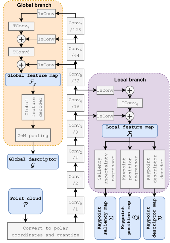
Figure 1: High-level architecture of EgoNN network. Numbers with a slash (e.g. /32) denote a stride of a feature map produced by each convolutional block in the network trunk.

The network has a 3D convolutional architecture shown in Fig. 1. The design is inspired by a successful MinkLoc3D [4] global point cloud descriptor. To improve the performance on larger point clouds, we increased the depth of the network and added channel attention (ECA [20]) to convolutional blocks. The bottom-up trunk consists of eight convolutional blocks $\mathrm{Conv}_{0},\ldots,\mathrm{Conv}_{7}$ producing sparse 3D feature maps with decreasing spatial resolution and increasing receptive field. Each convolutional block, starting from $\mathrm{Conv}_{1}$, decreases the spatial resolution by two. There are two top-down parts: global and local branch, both made of transposed 3D convolutions. Feature maps from higher pyramid levels, upsampled using transposed convolution (denoted $\mathrm{TConv}$), are added to the skipped features from the corresponding layer in the bottom-up trunk using lateral connections. Lateral connections apply convolutions with 1x1x1 kernel (denoted $\mathrm{1xConv}$) to unify the number of channels produced by bottom-up blocks before they are merged in the top-down pass. Such design produces feature maps with relatively high spatial resolution and a large receptive field, capturing high-level semantics of the input point cloud.

Global branch computes a global point cloud descriptor. It merges feature maps from higher pyramid levels to produce a global feature map $\mathcal{F}_{g}\in\mathbb{R}^{K\times 128}$. Each $\mathcal{F}_{g}$ element is processed by a global feature decoder, a two-layer MLP. The resulting 256-dimensional feature map is pooled with generalized-mean (GeM) [21] pooling to produce a global point cloud descriptor $\mathcal{G}\in\mathbb{R}^{256}$.

Local branch computes keypoints, their saliency uncertainty estimates, and descriptors. We adapt the approach proposed in USIP [22] for keypoint detection, which fits well with our architecture. The local branch merges feature maps from lower pyramid levels (level 3 and 4) to produce a local feature map $\mathcal{F}_{l}\in\mathbb{R}^{M\times 64}$. Each $\mathcal{F}_{l}$ element is processed by three heads. Keypoint position regressor, a two layer MLP followed by tanh function, computes keypoint coordinates map $\widehat{\mathcal{Q}}\in\left(-1,1\right)^{M\times 3}$. Saliency uncertainty regressor, a two layer MLP followed by a softplus, produces a keypoint uncertainty map $\Sigma\in\mathbb{R}_{+}^{M}$. Keypoint descriptor decoder, a two layer MLP, yields a keypoint descriptor map $\mathcal{D}\in\mathbb{R}^{M\times 128}$. $M$ is the number of supervoxels in the local feature map $\mathcal{F}_{l}$, that is the number of non-empty spatial locations in $\mathcal{F}_{l}$. In our implementation, supervoxel covers 8x8x8 voxels.

Keypoint position regressor outputs normalized keypoint cylindrical coordinates $\left(\hat{\rho},\hat{\theta},\hat{z}\right)\in\widehat{\mathcal{Q}}$ relative to the supervoxel center. One keypoint is regressed in each non-empty supervoxel. See Fig. 2 for illustration. To compute Cartesian keypoint coordinates $\mathcal{Q}$ we first transform them into absolute cylindrical coordinates $\left(\rho,\theta,z\right)$:

$$\rho=\frac{\hat{\rho}s_{\rho}}{2}+\rho_{c}\,,\theta=\frac{\hat{\theta}s_{\theta}}{2}+\theta_{c}\,,z=\frac{\hat{z}s_{z}}{2}+z_{c}\,,$$ (1)

where $s_{\rho},s_{\theta},s_{z}$ is the supervoxel size in each dimension and $\left(\rho_{c},\theta_{c},z_{c}\right)$ are absolute cylindrical coordinates of the supervoxel center. In our implementation local feature map $\mathcal{F}_{l}$ has a stride 8. So the supervoxel size in each direction is eight times the initial quantization step, that is $s_{\rho}=2.4\mathrm{m},s_{\theta}=8^{\circ},s_{z}=1.6\mathrm{m}$. Then, we transform cylindrical coordinates into Cartesian: $x=\rho\cos\theta$, $y=\rho\sin\theta$.

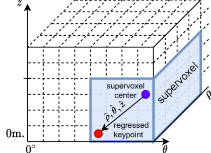
Figure 2: Illustration of the idea behind a keypoint position regressor. Cylindrical coordinates $\left(\hat{\rho},\hat{\theta},\hat{z}\right)$ of one keypoint relative to the supervoxel center are regressed in each non-empty supervoxel. Dashed lines indicate voxel boundaries.

Details of each network block are shown in Table I. $\mathrm{Conv}_{k}$ and $\mathrm{1Conv}$ blocks contain 3D convolutional layers; $\mathrm{TConv}_{k}$ are 3D transposed convolutions; MLP denotes a multi-layer perceptron with the number of neurons in each layer listed in parentheses.

TABLE I: Details of EgoNN architecture. BN=BatchNorm, MLP=Multi-Layer Perceptron.

Block	Layers
Bottom-up trunk
Conv0	32 filters 5x5x5 - BN - ReLU
Convk	$c_{k}$ filters 2x2x2 stride 2 - BN - ReLU
	$c_{k}$ filters 3x3x3 stride 1 - BN - ReLU
	$c_{k}$ filters 3x3x3 stride 1 - BN - ReLU
	ECA (Efficient Channel Attention)
where $c_{1}=32,c_{2}=c_{3}=64,c_{4}=c_{5}=c_{6}=c_{7}=128$
Global branch
TConvk, $k=6,7$	128 filters 2x2x2 stride 2
1xConv	128 filters 1x1x1 stride 1
Global feature	MLP(192, 256)
decoder
GeM pooling	Generalized-mean Pooling [21] layer
Local branch
TConvk, $k=4,5$	64 filters 2x2x2 stride 2
1xConv	64 filters 1x1x1 stride 1
Saliency uncertainty	MLP(32, 1) - Softplus
regressor
Keypoint position	MLP(32, 3) - Tanh
regressor
Keypoint descriptor	MLP(96, 128) - $L_{2}$-normalization
decoder

III-B Network Training

To reduce requirements for computational resources, each training step is split into two substeps. First, one mini-batch of training examples is used to calculate the loss on the global descriptor, and network weights are updated. Then, a different mini-batch is used to compute the loss on local features, and the network weights are updated again. Global part is trained using relatively large batches, allowing online mining of hard and informative training triplets. Local part training requires more GPU resources; thus, smaller batch size is used. Note that weights of the network trunk are optimized in both phases, as the gradient of both global and local losses backpropagates through them.

Global branch training substep. Mini-batches are constructed by sampling 128 pairs of similar point clouds. Two point clouds are considered similar if the distance between their centers, computed using the ground truth poses, is at most 2 m.

Mini-batch is processed by the network to compute a global descriptor $\mathcal{G}$ of each batch element, while the local branch is disabled. Mini-batch elements are arranged into triplets. For $i$-th batch element, we construct a training triplet $(i,p_{i},n_{i})$, where $i$ is an index of an anchor element, $p_{i}$ is an index of a point cloud similar to the anchor and $n_{i}$ is an index of a point cloud dissimilar to the anchor. Point clouds are dissimilar if the distance between their centers is above 10 m. We use the batch-hard mining [23] strategy to construct informative triplets and choose the hardest positive and negative examples within a batch. We augment training point clouds by removing points within a randomly selected cuboid, jittering point positions by adding Gaussian noise with $\sigma=0.1$, and applying random rotation around the z-axis.

We use a triplet margin loss [23] defined as:

$$\mathcal{L}_{G}(a_{i},p_{i},n_{i})=\max\left\{\left\lVert a_{i}-p_{i}\right\rVert_{2}-\left\lVert a_{i},n_{i}\right\rVert_{2}+m,0\right\},$$ (2)

where $a_{i},p_{i},n_{i}$ are embeddings of an anchor, a positive and negative elements in $i$-th training triplet and $m=0.2$ is a margin hyperparameter.

Local branch training substep. In each training step, we sample a pair of similar point clouds, that is point clouds with at most 2 m distance between their centers. We augment training point clouds by random rotation around the z-axis and random translation in the x-y plane up to 5 m.

Sampled mini-batch is processed by the network to compute keypoint descriptor map $\mathcal{D}$, keypoint position map $\mathcal{Q}$ and saliency uncertainty map $\Sigma$ for each batch element. The global branch is switched off.

The local loss function $\mathcal{L}_{L}$ is a sum of three terms: two keypoint-related losses $\mathcal{L}_{C}$, $\mathcal{L}_{P2P}$ and a local descriptor loss $\mathcal{L}_{D}$:

$$\mathcal{L}=\lambda_{C}\mathcal{L}_{C}+\lambda_{P2P}\mathcal{L}_{P2P}+\lambda_{D}\mathcal{L}_{D},$$ (3)

where $\lambda_{C}=1,\lambda_{P2P}=1,\lambda_{D}=1\in\mathbb{R}_{+}$ are experimentally chosen hyperparameters.

Keypoint-related loss. To compute the keypoints position, we adapt the approach proposed in USIP [22]. One keypoint is regressed in each non-empty supervoxel (see Fig. 2). To get repeatable keypoints, each keypoint regressed in the first point cloud (in the area overlapping with the second point cloud) should have a corresponding keypoint detected in the second cloud. Additionally, a position of the regressed keypoint should be close to some 3D point in the input cloud. To enforce these constraints, the keypoint loss is a sum of two terms: $\mathcal{L}_{C}$ is the probabilistic chamfer loss [22] that minimizes the probabilistic distances between corresponding pairs of keypoints in two point clouds. It drives corresponding keypoints to be as close as possible, taking into account their saliency uncertainty. $\mathcal{L}_{P2P}$ is the point-to-point loss that minimizes the distance between regressed keypoints and their nearest neighbors in the point cloud. See USIP [22] for derivation and discussion on keypoint-related loss terms. Let $\mathcal{Q}=\left\{\mathrm{q}_{1},\ldots,\mathrm{q}_{N}\right\}$ and $\widetilde{\mathcal{Q}}=\left\{\widetilde{\mathrm{q}}_{1},\ldots,\widetilde{\mathrm{q}}_{M}\right\}$, be sets of keypoint Cartesian coordinates computed for a pair of overlapping point clouds. $\Sigma=\left\{\sigma_{1},\ldots,\sigma_{N}\right\},\sigma_{i}\in\mathbb{R}_{+}$ and $\widetilde{\Sigma}=\left\{\widetilde{\sigma}_{1},\ldots,\widetilde{\sigma}_{M}\right\}_{i=1}^{M},\widetilde{\sigma}_{i}\in\mathbb{R}_{+}$ their saliency uncertainty estimates. $\mathcal{Q}^{\prime}=\left\{\mathrm{q}^{\prime}_{1},\ldots,\mathrm{q}^{\prime}_{M}\right\}$ is the set of keypoints in the second point cloud $\widetilde{\mathcal{Q}}$ brought to the first point cloud coordinate frame, using the ground truth transform $\mathrm{T}$, $\mathcal{Q}^{\prime}=\mathrm{T}^{-1}\circ\widetilde{\mathcal{Q}}$.

Probabilistic chamfer loss [22] $\mathcal{L}_{\mathrm{c}}$ is defined as:

$$\mathcal{L}_{C}=\sum_{i=1}^{N}\left(\ln s_{i}+\frac{d_{i}}{s_{i}}\right)+\sum_{j=1}^{M}\left(\ln s^{\prime}_{j}+\frac{d^{\prime}_{j}}{s^{\prime}_{j}}\right),$$ (4)

where $d_{i}=\left\lVert\mathrm{q}_{i}-\mathrm{q}^{\prime}_{nn(i)}\right\rVert_{2}$ and $d^{\prime}_{j}=\left\lVert\mathrm{q}^{\prime}_{j}-\mathrm{q}_{nn^{\prime}(j)}\right\rVert_{2}$ are Euclidean distances between corresponding keypoints detected in two point clouds; $s_{i}=\frac{1}{2}\left(\sigma_{i}+\widetilde{\sigma}_{nn(i)}\right)$, $s^{\prime}_{j}=\frac{1}{2}\left(\widetilde{\sigma_{j}}+\sigma_{nn^{\prime}(j)}\right)$ are mean saliency uncertainties of corresponding keypoints; $nn(i)=\arg\min_{j}\left\lVert\mathrm{q}_{i}-\mathrm{q}^{\prime}_{j}\right\rVert_{2}$ is the index of the keypoint in the second point cloud corresponding to the $i$-th keypoint in the first point cloud and $nn^{\prime}(j)=\arg\min_{i}\left\lVert\mathrm{q}^{\prime}_{j}-\mathrm{q}_{i}\right\rVert_{2}$ is the index of the keypoint in the first point cloud corresponding to the $j$-th keypoint in the second point cloud.

Point-to-point loss $\mathcal{L}_{\mathrm{p2p}}$ is defined as:

$$\mathcal{L}_{P2P}=\sum_{i=1}^{N}\min_{\mathrm{p}_{j}\in\mathcal{P}}\left\lVert\mathrm{q}_{i}-\mathrm{p}_{j}\right\rVert_{2}+\sum_{j=1}^{M}\min_{\widetilde{\mathrm{p}}_{i}\in\widetilde{\mathcal{P}}}\left\lVert\widetilde{\mathrm{q}}_{j}-\widetilde{\mathrm{p}_{i}}\right\rVert_{2},$$ (5)

where each of two terms is a sum of distances between regressed keypoints and their nearest neighbours in the input point cloud.

Local descriptors-related loss. We compute local descriptors not for all points in the input cloud but for a much smaller, typically by an order of magnitude, set of regressed keypoints. This allows efficient processing of relatively large points clouds. Similarly as in [19], keypoint correspondence is posed as a multi-class classification problem, where a point in the first cloud is classified as corresponding to one point in the second cloud. To cater for partial correspondence, we filter out keypoints in the first point cloud without corresponding points in the second cloud, based on a known ground truth alignment. $\mathcal{D^{\prime}}\in\mathbb{R}^{N^{\prime}\times d}$ is a filtered local descriptors matrix in the first point cloud. $C=\mathcal{D^{\prime}}\widetilde{\mathcal{D}}^{T}\in\mathbb{R}^{N^{\prime}\times M}$ denotes a correspondence matrix between local descriptors in two point clouds, where $C_{ij}\in\left[-1,1\right]$ is a cosine similarity between descriptors $i$ and $j$. We use cross-entropy loss function defined as:

$$\mathcal{L}_{D}=-\frac{1}{N^{\prime}}\sum_{i=1}^{N^{\prime}}\log\left(\frac{\exp\left(C_{i,nn(i)}/\tau\right)}{\sum_{j=1}^{M}\exp\left(C_{i,j}/\tau\right)}\right)\,,$$ (6)

where $nn(i)$ is the index of the keypoint in the second point cloud corresponding to the $i$-th keypoint in the first point cloud based on a ground truth pose, and $\tau=0.02$ is a temperature hyperparameter.

Implementation details. All experiments are performed on a server with a single nVidia RTX 2080Ti GPU, 12 core AMD Ryzen Threadripper 1920X processor, 64 GB of RAM, and SSD hard drive. We use PyTorch 1.9 [24] deep learning framework, MinkowskiEngine 0.5.4 [25] auto-differentiation library for sparse tensors, PML Pytorch Metric Learning library 0.9.99 [26], and efficient RANSAC and ICP implementations from Open3D 0.13.0 [27] library.

IV Experimental Results

IV-A Datasets and Evaluation Methodology

Our model is trained and evaluated using disjoint subsets of two large-scale datasets MulRan [28] and Apollo-SouthBay [29]. Moreover, we test generalization abilities on the KITTI odometry dataset [30].

MulRan dataset [28] is gathered by a vehicle traveling through different trajectories in South Korea. Point clouds are acquired using Ouster OS1-64 rotating LiDAR with 120 m range and contain about 60k points. Each trajectory is traversed multiple times, at different times of day or year, to allow realistic evaluation of place recognition methods. To speed up the processing, we remove uninformative ground plane points with z coordinate below $-0.9$ m. The dataset contains timestamped 6DoF ground-truth poses for each traversal estimated using VRS-GPS/INS integrated navigation system and a graph SLAM. The longest and most diverse trajectory, Sejong, is split into disjoint training and evaluation parts.

Apollo-SouthBay dataset [29] is collected during multiple traversals through six different routes in the southern San Francisco Bay Area. The dataset covers various environments, such as residential areas, urban downtown areas, and highways. The data is acquired using Velodyne HDL-64E rotating LiDAR with a similar range and number of scanned 3D points as in the MulRan dataset. We remove points on the ground plane level with z coordinate below $-1.6$ m. Ground truth 6DoF poses are acquired by postprocessing readings from a high-end GNSS RTK/INS integrated navigation system. The longest and most diverse trajectory (SunnyvaleBigLoop) is used for evaluation. The other five shorter trajectories are included in the training split.

Kitti odometry dataset [30] is acquired using a vehicle driving around the mid-size city of Karlsruhe, in rural areas, and on highways. It contains 11 sequences with LiDAR point clouds and ground truth poses. The data is acquired with the same Velodyne HDL-64E LiDAR as used in the Apollo-SouthBay dataset. $1.5$ m threshold on the z-coordinate is used to remove ground plane points. Ground truth poses are acquired using a high-end GNSS RTK/INS integrated navigation system. We evaluate our approach on a sequence 00 as it contains the highest number of loops. We build a map from the first 170 seconds of the sequence and leave the rest for queries.

To avoid processing multiple scans of the same place when the vehicle doesn’t move, we ignore consecutive readings with less than 20 cm displacement. Details of the training and evaluation splits are given in Tab. II. In all three datasets, we observed that ground truth 6DoF poses between different traversals through the same trajectory are slightly misaligned. Therefore, we use an ICP [16] to refine 6DoF poses between pairs of point clouds from different traversals.

TABLE II: Details of training and evaluation sets.

	Split	Length	Number of scans
MulRan: Sejong	train	19 km	$35.9$k
SouthBay: excl. Sunnyvale	train	37 km	$72.7$k
MulRan: Sejong	test	4 km	$3.8$k / $3.5$k (map / query)
SouthBay: Sunnyvale	test	38 km	$49.0$k / $17$k (map / query)
Kitti: Sequence 00	test	4 km	$1.6$k / $0.6$k (map / query)

IV-A1 Evaluation Metrics.

To evaluate the performance of the global descriptor, we follow a similar evaluation protocol as in [2, 3]. Each evaluation set is split into two parts: a query and a database set, covering the same geographic area. A query is formed from point clouds acquired during one traversal, and the database is built from data gathered on a different day. For each query point cloud, we find in the database candidate point clouds with the closest, in Euclidean distance sense, global descriptors. Localization is successful if at least one of the top $N$ candidates is within $d$ meters threshold from the query ground truth position. Recall@N is defined as the percentage of correctly localized queries. We report Recall@1 (R@1) and Recall@5 (R@5) metrics for $d=5$ and $20$ m thresholds.

We use a simple two-step localization procedure to evaluate the performance of 6DoF pose estimation. First, for each query point cloud, we perform the coarse localization by searching the database for a point cloud with the closest global descriptor. Since this work focuses on efficient keypoint and descriptor extraction, we do not consider more sophisticated approaches, where more database candidates are examined. If the coarse localization is successful, that is if the returned point cloud is within 20 m threshold from the ground truth query position, we estimate 6DoF relative pose between the query and the database point cloud. If the coarse localization fails, we exclude the query point cloud from further evaluation. From the query and database point cloud, we select 128 keypoints with the lowest saliency uncertainty ($\Sigma$). We match selected keypoints in both clouds using their local descriptors and estimate their relative pose with RANSAC [31]. We report the 6DoF pose estimation success if an estimated pose is within 2 m and $5^{\circ}$ threshold from the ground truth. We calculate an average relative rotation error (RRE) and relative translation error (RTE) for successful pose estimation events.

IV-B Results and Discussion

Comparison with state of the art. We compare our method with handcrafted M2DP [9], ScanContext [10] and learned MinkLoc3D [4], Disco [5] global descriptors; FCGF [32] and D3Feat [33] local descriptors and combined local and global DH3D [3] descriptor. We re-trained MinkLoc3D, DiSCO, and DH3D using a publicly released code and the same training sets as our method. For FCGF and D3Feat we use publicly available models trained on Kitti. Except for M2DP, the same preprocessing is used, that is points on and below the ground plane level are removed based on the z coordinate.

Table III shows coarse-level place recognition results using a global descriptor. Our EgoNN method outperforms other descriptors on all three datasets. The highest advantage is for the MulRan dataset (Recall@1 with 5 m threshold is almost 4 pp above runner-up DiSCO). On other evaluation sets our method has a smaller but consistent advantage over the runner-up.

Table IV shows 6DoF pose estimation results. For FCGF and D3Feat local descriptors, we first use a global descriptor computed by EgoNN to find the closest point cloud in the database. Our method has a high success ratio (above 99.6% for MulRan and Kitti and above 97% for SouthBay). For these successful cases, the mean relative translation error (RTE) is between 12-19 cm and the rotation error (RRE) is between 0.3-0.4^∘. Our method outperforms the other integrated local and global descriptor, DH3D, by a large margin. Poor DH3D performance can be explained by the fact that it was designed to process smaller point clouds. Specialized local descriptors, FCGF and D3Feat, achieve slightly lower pose estimation errors, but at the expense of larger running times (see Runtime analysis section).

TABLE III: Results of a coarse localization using a global descriptor. Recall@1 and Recall@5 are reported with 5 and 20 m thresholds.

	MulRan				Apollo-SouthBay				Kitti
	5 m thresh.		20 m thresh.		5 m thresh.		20 m thresh.		5 m thresh.		20 m thresh.
	R@1	R@5	R@1	R@5	R@1	R@5	R@1	R@5	R@1	R@5	R@1	R@5
M2DP [9]	0.441	0.556	0.595	0.688	-	-	-	-	0.945	0.953	0.945	0.953
ScanContext [10]	0.861	0.896	0.885	0.915	0.910	0.910	0.921	0.924	0.963	0.973	0.963	0.964
MinkLoc3D [4]	0.823	0.944	0.921	0.966	0.772	0.938	0.950	0.983	0.957	0.969	0.977	0.980
DiSCO [5]	0.940	0.975	0.958	0.981	0.951	0.966	0.954	0.970	0.907	0.913	0.923	0.945
DH3D [3]	0.324	0.562	0.589	0.755	0.253	0.496	0.504	0.707	0.755	0.911	0.868	0.961
EgoNN (ours)	0.983	0.999	0.996	0.999	0.957	0.977	0.963	0.982	0.974	0.982	0.979	0.987

TABLE IV: Results of a 6DoF pose estimation using local features within 2 m and $5^{\circ}$ threshold. RTE=relative translation error, RRE=relative rotation error.

	MulRan			Apollo-SouthBay			Kitti
	Success (%)	RTE (cm)	RRE (∘)	Success (%)	RTE (cm)	RRE (∘)	Success (%)	RTE (cm)	RRE (∘)
EgoNN+FCGF [32]	0.965	18	0.4	0.943	13	0.4	0.966	10	0.3
EgoNN+D3Feat [33]	0.991	16	0.4	0.975	12	0.3	0.998	7	0.2
DH3D [3]	0.563	41	1.3	0.614	55	0.9	0.932	26	0.6
EgoNN (ours)	0.996	19	0.4	0.970	15	0.4	0.997	12	0.3

Robustness to viewpoint changes. Figure 3 shows the robustness of our global descriptor to viewpoint changes. Plots show Recall@1 with 5 m threshold (y-axis) on MulRan evaluation set for different magnitudes of a random rotation (x-axis) of a query point cloud. A blue line corresponds to our EgoNN method using cylindrical coordinates and random rotation augmentation during the training. The global descriptor is invariant to the point cloud rotation. Using Cartesian coordinates yields over 8 pp worse Recall@1 even without applying any rotation. Due to the translational invariance of convolutional filters, a small point cloud translation has less effect on the global descriptor when using Cartesian coordinates instead of cylindrical. Thus, the nearest neighbor search in the descriptor space more likely returns more distant candidates. This deteriorates Recall@1 metric with a small 5 m threshold. Using only cylindrical coordinates, without random rotation augmentation, produces a descriptor highly sensitive to the point cloud orientation. Without random rotation augmentation, rotations still affects convolutional filter responses at the borders (in regions with $\theta$ coordinate near $0$ or $2\pi$).

Figure 4 shows 6DoF pose estimation success ratio within 2 m and $5^{\circ}$ threshold as a function of an initial orientation of two point clouds. Both point-to-point and point-to-plane ICP [16] variants are sensitive to an initial point cloud alignment. Success ratio starts dropping down when initial orientation difference is larger than $20^{\circ}$. On the other hand, using EgoNN keypoints and descriptors with RANSAC allows successful 6DoF pose estimation despite a large initial misalignment. Examples are visualized in Fig. 5. It show point cloud pairs gathered during revisiting same places from different directions in the Kitti dataset. In all three cases, 6DoF pose estimation error was below 16 cm and $0.8^{\circ}$, whereas ICP registration failed and got stuck in a local minima due to a large initial misalignment.

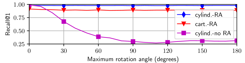
Figure 3: Impact of a coordinate system choice (cylindrical vs. Cartesian) and training data augmentation (RA = random rotation) on the global descriptor rotational invariance. Plots show Recall@1 with 5 m threshold for different angles of the orientation difference between two point clouds.

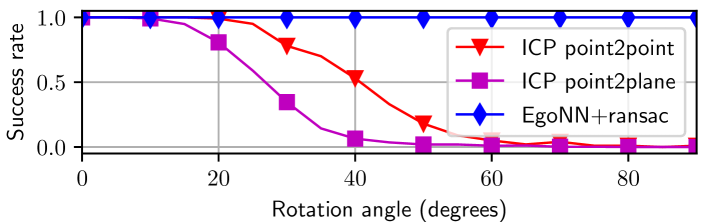
Figure 4: Impact of an initial point cloud alignment on the registration success ratio. Plots show 6DoF pose estimation success ratio (with 2 m and $5^{\circ}$ threshold) for different angles of the query point cloud rotation.

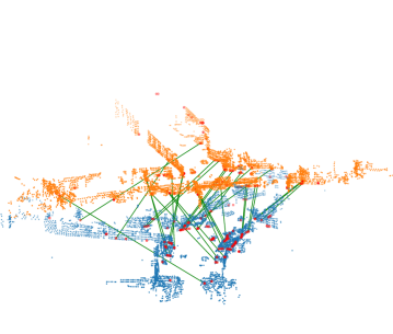
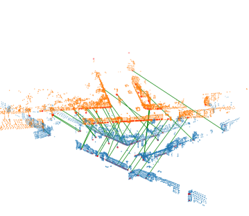
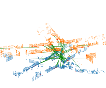
Figure 5: Successful registration of the exemplary point clouds gathered during revisiting the same place from different directions in the Kitti dataset using EgoNN with RANSAC. Green lines connect corresponding keypoints (RANSAC inliers).

Keypoint detection. Figure 6 shows 128 keypoints with the lowest saliency uncertainty $\Sigma$ detected in an exemplary point cloud. It can be seen that keypoints are detected at distinctive locations, such as the bottom of tree trunks. The repeatability of keypoint detector is examined in Figure 7. A keypoint is repeatable if, in the other point cloud aligned using the ground truth transform, another keypoint is detected within 0.5 m threshold. Our method generates highly repeatable keypoints. When 64 keypoints with the lowest saliency uncertainty $\Sigma$ are selected, repeatability is as high as 65% and decreases to 37% for 1024 most salient keypoints.

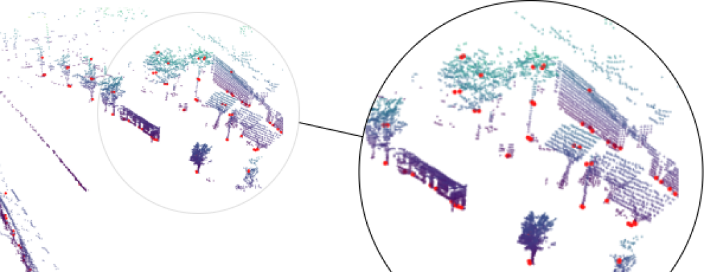
Figure 6: Visualization of keypoint detection results, showing 128 points with the lowest saliency uncertainty.

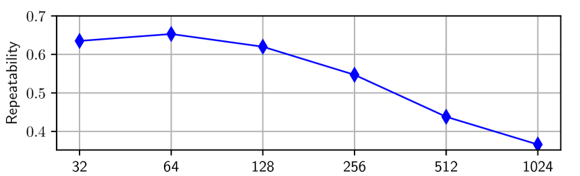
Figure 7: Repeatability when a different number of keypoints with the lowest saliency uncertainty is chosen.

Ablation study results are shown in Table V. The top row shows the performance of our method on the MulRan evaluation set. Lower rows show results with parts of the network removed or disabled. Simplifying the network architecture by removing the top-down processing path (no top-down blocks), containing blocks Conv₆, Conv₇ TConv₆, TConv₇, TConv₄, lowers the coarse localization performance by 3-5 p.p. Disabling keypoint saliency uncertainty estimation (no saliency regress.), and selecting 128 random keypoints instead of keypoints with the lowest uncertainty, almost doubles relative translation error and increases rotation error by 50%. Removing the keypoint position regressor (no position regress.), and assuming keypoint locations at the supervoxel centers, further degrades the performance of 6DoF pose estimation.

TABLE V: Ablation study. The top row is a full EgoNN model. Lower rows show the performance of reduced architectures.

	COARSE LOC.		6DoF POSE EST.
	5 m	20 m	2 m and $5^{\circ}$ threshold
	R@1	R@1	Succ.(%)	RTE(cm)	RRE(∘)
EgoNN	0.983	0.996	0.996	19	0.4
no top-down blocks	0.934	0.964	0.989	19	0.4
no saliency regress.	0.983	0.996	0.988	34	0.6
no position regress.	0.983	0.996	0.854	67	0.8

Runtime analysis. EgoNN requires 28 ms for extraction of global descriptor and local keypoints from a point cloud with 30k points. Other method extracting both global and local descriptors, DH3D [3], requires 78 ms. Local descriptor extraction methods require much longer time: 360  ms for FCGF [32] and 130 ms for D3Feat [33]. Methods extracting only a global descriptor are faster: 8 ms for ScanContext, 10 ms for DiSCO, 14 ms for MinkLoc3D and 22 ms for M2DP. But 10-20 ms extra time needed by EgoNN is acceptable, as it additionally produces repetitive keypoints and discriminative local descriptors allowing a robust 6DoF pose estimation. It takes only 5 ms to match 128 keypoints with the lowest saliency uncertainty and estimate 6DoF pose between two point clouds with RANSAC.

The efficiency of EgoNN can be attributed to three factors. First, computations during a local and global descriptor extraction are shared. Second, we do not compute local descriptors for all 3D points, but only for much lower number of detected keypoints. Third, using sparse voxelized representation and relatively simple convolutional architecture allows efficient processing with MinkowskiEngine [25] auto-differentiation library for sparse tensors.

V Conclusion

This paper presents EgoNN, a 3D convolutional architecture based on a sparse voxelized representation, to efficiently extract global and local descriptors from large point clouds acquired using a modern 3D rotating LiDAR. Experimental evaluation proves that our global descriptor outperforms prior cloud-based place recognition methods. Local descriptors allow efficient 6DoF pose estimation within 19 cm and 0.4^∘ degree accuracy. For simplicity, we evaluated the performance of a coarse localization using only global descriptors. A potential research direction is to investigate how the localization accuracy can be improved by re-ranking candidate locations using local keypoints and descriptors.

References

- [1] X. Chen, T. Läbe, A. Milioto, T. Röhling, O. Vysotska, A. Haag, J. Behley, C. Stachniss, and F. Fraunhofer, “Overlapnet: Loop closing for lidar-based slam,” in Proc. of Robotics: Science and Systems (RSS), 2020.
- [2] M. A. Uy and G. H. Lee, “Pointnetvlad: Deep point cloud based retrieval for large-scale place recognition,” in Proceedings of the IEEE Conference on Computer Vision and Pattern Recognition, 2018, pp. 4470–4479.
- [3] J. Du, R. Wang, and D. Cremers, “Dh3d: Deep hierarchical 3d descriptors for robust large-scale 6dof relocalization,” in European Conference on Computer Vision. Springer, 2020, pp. 744–762.
- [4] J. Komorowski, “Minkloc3d: Point cloud based large-scale place recognition,” in Proceedings of the IEEE/CVF Winter Conference on Applications of Computer Vision (WACV), January 2021, pp. 1790–1799.
- [5] X. Xu, H. Yin, Z. Chen, Y. Li, Y. Wang, and R. Xiong, “Disco: Differentiable scan context with orientation,” IEEE Robotics and Automation Letters, 2021.
- [6] J. Knopp, M. Prasad, G. Willems, R. Timofte, and L. Van Gool, “Hough transform and 3d surf for robust three dimensional classification,” in European Conference on Computer Vision. Springer, 2010, pp. 589–602.
- [7] F. Tombari, S. Salti, and L. Di Stefano, “A combined texture-shape descriptor for enhanced 3d feature matching,” in 2011 18th IEEE international conference on image processing. IEEE, 2011, pp. 809–812.
- [8] B. Steder, M. Ruhnke, S. Grzonka, and W. Burgard, “Place recognition in 3d scans using a combination of bag of words and point feature based relative pose estimation,” in 2011 IEEE/RSJ International Conference on Intelligent Robots and Systems. IEEE, 2011, pp. 1249–1255.
- [9] L. He, X. Wang, and H. Zhang, “M2dp: A novel 3d point cloud descriptor and its application in loop closure detection,” in 2016 IEEE/RSJ International Conference on Intelligent Robots and Systems (IROS). IEEE, 2016, pp. 231–237.
- [10] G. Kim and A. Kim, “Scan context: Egocentric spatial descriptor for place recognition within 3d point cloud map,” in 2018 IEEE/RSJ International Conference on Intelligent Robots and Systems (IROS). IEEE, 2018, pp. 4802–4809.
- [11] Y. Fan, Y. He, and U.-X. Tan, “Seed: A segmentation-based egocentric 3d point cloud descriptor for loop closure detection,” in 2020 IEEE/RSJ International Conference on Intelligent Robots and Systems (IROS). IEEE, 2020, pp. 5158–5163.
- [12] X. Cai and W. Yin, “Weighted scan context: Global descriptor with sparse height feature for loop closure detection,” in 2021 International Conference on Computer, Control and Robotics (ICCCR). IEEE, 2021, pp. 214–219.
- [13] Y. Wang, Z. Sun, C.-Z. Xu, S. Sarma, J. Yang, and H. Kong, “Lidar iris for loop-closure detection,” arXiv preprint arXiv:1912.03825, 2019.
- [14] Z. Liu, S. Zhou, C. Suo, P. Yin, W. Chen, H. Wang, H. Li, and Y.-H. Liu, “Lpd-net: 3d point cloud learning for large-scale place recognition and environment analysis,” in Proceedings of the IEEE International Conference on Computer Vision, 2019, pp. 2831–2840.
- [15] L. Schaupp, M. Bürki, R. Dubé, R. Siegwart, and C. Cadena, “Oreos: Oriented recognition of 3d point clouds in outdoor scenarios,” in 2019 IEEE/RSJ International Conference on Intelligent Robots and Systems (IROS), 2019, pp. 3255–3261.
- [16] P. J. Besl and N. D. McKay, “Method for registration of 3-d shapes,” in Sensor fusion IV: control paradigms and data structures, vol. 1611. International Society for Optics and Photonics, 1992, pp. 586–606.
- [17] Y. Wang and J. M. Solomon, “Deep closest point: Learning representations for point cloud registration,” in Proceedings of the IEEE/CVF International Conference on Computer Vision, 2019, pp. 3523–3532.
- [18] Z. J. Yew and G. H. Lee, “Rpm-net: Robust point matching using learned features,” in Proceedings of the IEEE/CVF conference on computer vision and pattern recognition, 2020, pp. 11 824–11 833.
- [19] T. Zodage, R. Chakwate, V. Sarode, R. A. Srivatsan, and H. Choset, “Correspondence matrices are underrated,” in 2020 International Conference on 3D Vision (3DV), 2020, pp. 603–612.
- [20] Q. Wang, B. Wu, P. Zhu, P. Li, W. Zuo, and Q. Hu, “Eca-net: Efficient channel attention for deep convolutional neural networks, 2020 ieee,” in CVF Conference on Computer Vision and Pattern Recognition (CVPR). IEEE, 2020.
- [21] F. Radenović, G. Tolias, and O. Chum, “Fine-tuning cnn image retrieval with no human annotation,” IEEE transactions on pattern analysis and machine intelligence, vol. 41, no. 7, pp. 1655–1668, 2018.
- [22] J. Li and G. H. Lee, “Usip: Unsupervised stable interest point detection from 3d point clouds,” in Proceedings of the IEEE/CVF International Conference on Computer Vision, 2019, pp. 361–370.
- [23] A. Hermans, L. Beyer, and B. Leibe, “In defense of the triplet loss for person re-identification,” arXiv preprint arXiv:1703.07737, 2017.
- [24] A. Paszke et al., “Pytorch: An imperative style, high-performance deep learning library,” in Advances in Neural Information Processing Systems 32, H. Wallach et al., Eds. Curran Associates, Inc., 2019, pp. 8024–8035.
- [25] C. Choy, J. Gwak, and S. Savarese, “4d spatio-temporal convnets: Minkowski convolutional neural networks,” in Proceedings of the IEEE Conference on Computer Vision and Pattern Recognition, 2019, pp. 3075–3084.
- [26] K. Musgrave, S. Belongie, and S.-N. Lim, “A metric learning reality check,” arXiv preprint arXiv:2003.08505, 2020.
- [27] Q.-Y. Zhou, J. Park, and V. Koltun, “Open3d: A modern library for 3d data processing,” arXiv preprint arXiv:1801.09847, 2018.
- [28] G. Kim, Y. S. Park, Y. Cho, J. Jeong, and A. Kim, “Mulran: Multimodal range dataset for urban place recognition,” in Proceedings of the IEEE International Conference on Robotics and Automation (ICRA), Paris, May 2020.
- [29] W. Lu, Y. Zhou, G. Wan, S. Hou, and S. Song, “L3-net: Towards learning based lidar localization for autonomous driving,” in Proceedings of the IEEE Conference on Computer Vision and Pattern Recognition, 2019, pp. 6389–6398.
- [30] A. Geiger, P. Lenz, and R. Urtasun, “Are we ready for autonomous driving? the kitti vision benchmark suite,” in Conference on Computer Vision and Pattern Recognition (CVPR), 2012.
- [31] M. A. Fischler and R. C. Bolles, “Random sample consensus: a paradigm for model fitting with applications to image analysis and automated cartography,” Communications of the ACM, vol. 24, no. 6, pp. 381–395, 1981.
- [32] C. Choy, J. Park, and V. Koltun, “Fully convolutional geometric features,” in Proceedings of the IEEE/CVF International Conference on Computer Vision, 2019, pp. 8958–8966.
- [33] X. Bai, Z. Luo, L. Zhou, H. Fu, L. Quan, and C.-L. Tai, “D3feat: Joint learning of dense detection and description of 3d local features,” in Proceedings of the IEEE/CVF Conference on Computer Vision and Pattern Recognition, 2020, pp. 6359–6367.