Micro Batch Streaming: Allowing the Training of DNN Models to Use a large Batch Size in Memory Constrained Environments

Abstract

Recent deep learning models are difficult to train using a large batch size, because commodity machines may not have enough memory to accommodate both the model and a large data batch size. The batch size is one of the hyper-parameters used in the training model, and it is dependent on and is limited by the target machine memory capacity because the batch size can only fit into the remaining memory after the model is uploaded. Moreover, the data item size is also an important factor because if each data item size is larger then the batch size that can fit into the remaining memory becomes smaller. This paper proposes a framework called Micro-Batch Streaming (MBS) to address this problem. This method helps deep learning models to train by providing a batch streaming method that splits a batch into a size that can fit in the remaining memory and streams them sequentially. A loss normalization algorithm based on the gradient accumulation is used to maintain the performance. The purpose of our method is to allow deep learning models to train using larger batch sizes that exceed the memory capacity of a system without increasing the memory size or using multiple devices (GPUs).

1 Introduction

Recently, many research use heavy Deep Neural Network (DNN) models that need a lot of memory to execute. Plus, data sizes are increasing such that it is difficult to increase the mini-batch size which is used for the training of the models. The mini-batch size is an important hyper-parameter that determines the number of data set items that are used in one iteration of a training process and the mini-batch size may affect the overall performance of the DNN as shown in [1]. The results in table 1 show the comparison between a large mini-batch and a small mini-batch used for the image classification and semantic segmentation problems. Utilizing a large mini-batch shows 21.88% and 2.01% higher than a small mini-batch when using higher resolution images for image classification and semantic segmentation problems, respectively.

The image size may also affect the model performance, because the image size may limit the mini-batch size. Also, higher resolution images (i.e., larger image size) contain more information about objects. Table 1 shows the comparison of results between the higher resolution images and the lower resolution images that are used for the image classification and semantic segmentation problems. Using the higher resolution image data shows 21.64% and 2.01% higher than the lower resolution image data in a large mini-batch for image classification and semantic segmentation problems, respectively. This aspect is also similar when using a small mini-batch size.

Table 1: The effect of batch size and image size for a image classification model (ResNet-50) using Flower-102 dataset and a semantic segmentation model (U-Net) using Carvana dataset.

Model		ResNet-50		U-Net
Metric		Max. acc (%)		Max. IoU (%)
Image size		32$\times$32	224$\times$224	96$\times$96	384$\times$384
Batch	2	48.66	61.86	92.30	93.61
Size	16	62.10	83.74	93.61	95.62

The total memory size of a mini-batch can only be increased to the remaining memory after the model is loaded. Thus, there is a limit on the size of the mini-batch and the number of data items included in the mini-batch. If the memory requirement of a certain mini-batch size is larger than the free remaining memory size, the mini-batch cannot be allocated to the GPU memory and the model cannot be trained. If the optimal mini-batch size for a particular resolution dataset is larger than the device memory, then the mini-batch size must be reduced when increasing the image resolution or use low-resolution image data to increase the mini-batch size. Therefore, the significant increase in image size makes it more challenging to train DNN models.

Many researchers tried various techniques such as data parallelism and/or model parallelism to alleviate the problems that deep learning methods face. Data parallelism (e.g., [2, 3, 4]) is usually used when the mini-batch size is too large to be fit into a single device’s memory. A mini-batch is partitioned for computation and scattered to multiple devices and each device has a full copy of the learning model. When all data within a mini-batch is processed, weights are updated across devices through communications. Model parallelism partitions the learning model into cells and distributes the cells to multiple devices. It is usually used when the model is too large to fit into a device’s memory (e.g., [5, 6, 7]). Other methods that use pipeline parallelism are proposed (e.g., [8, 9]). These methods employ Data-Parallel Synchronous Stochastic Gradient Descent (SGD), which distributes mini-batches across many machines in unit of micro-batches and executes them in a pipelined fashion. Although, all of these research improve the learning and performance of the models, they still have the problem of the mini-batch size being limited by the device memory size.

This paper proposes the Micro-Batch Streaming (MBS), which is a method that can fetch a large batch of data using the stream-based pipeline scheme to train models even if the batch cannot fit into the memory without increasing the device memory or using multiple devices (GPUs). Thus, allowing researchers to experiment using large mini-batch sizes on a single device. The idea is to split a mini-batch into $n$ micro-batches ([8, 9])and stream them sequentially to a GPU. Results show that MBS can increase the training batch size to the full size of the training set regardless of the model type, dataset, and data size. To maintain the performance, MBS computes the gradient for a large batch using loss normalization based on micro-batch gradient accumulation, a method that accumulates the gradient of multiple micro-batches.

This paper is organized as follows. Related work is described in Section 2. Section 3 introduces MBS and terminologies used throughout this paper is described, and the loss normalization algorithm used to maintain the performance is introduced. Section 4 depicts the results. Finally, Section 5 concludes the paper.

2 Related work

If model parallelism is done naively, GPUs suffer from idle time overhead because a worker have to wait for previous or successor worker to finish its job. To minimize this overhead, GPipe [8], a model-parallelism library for training large neural networks, presented a novel pipeline parallelism with batch splitting. GPipe splits mini-batch into smaller batches, called micro-batch, for pipeline execution across multiple GPUs. This enables each GPU to work on different micro-batch simultaneously, and gradient and model parameters are updated synchronously after all micro-batches are processed. However, synchronizing at the end of every mini-batch still causes GPU to stall. Pipedream [9] used asynchronous communication method and corresponding work scheduling and learning method to handle this problem. But neither of these solutions are adequate for large mini-batch training because they focus on maximizing the learning performance or parallelization of the learning process. Plus, they have a limitation where the batch size cannot exceed the free memory space as the physical memory does not have infinite capacity. The proposed method in this paper solves this limitation without increasing the memory of a single device and without using multiple devices (GPUs)

3 Micro-Batch Streaming

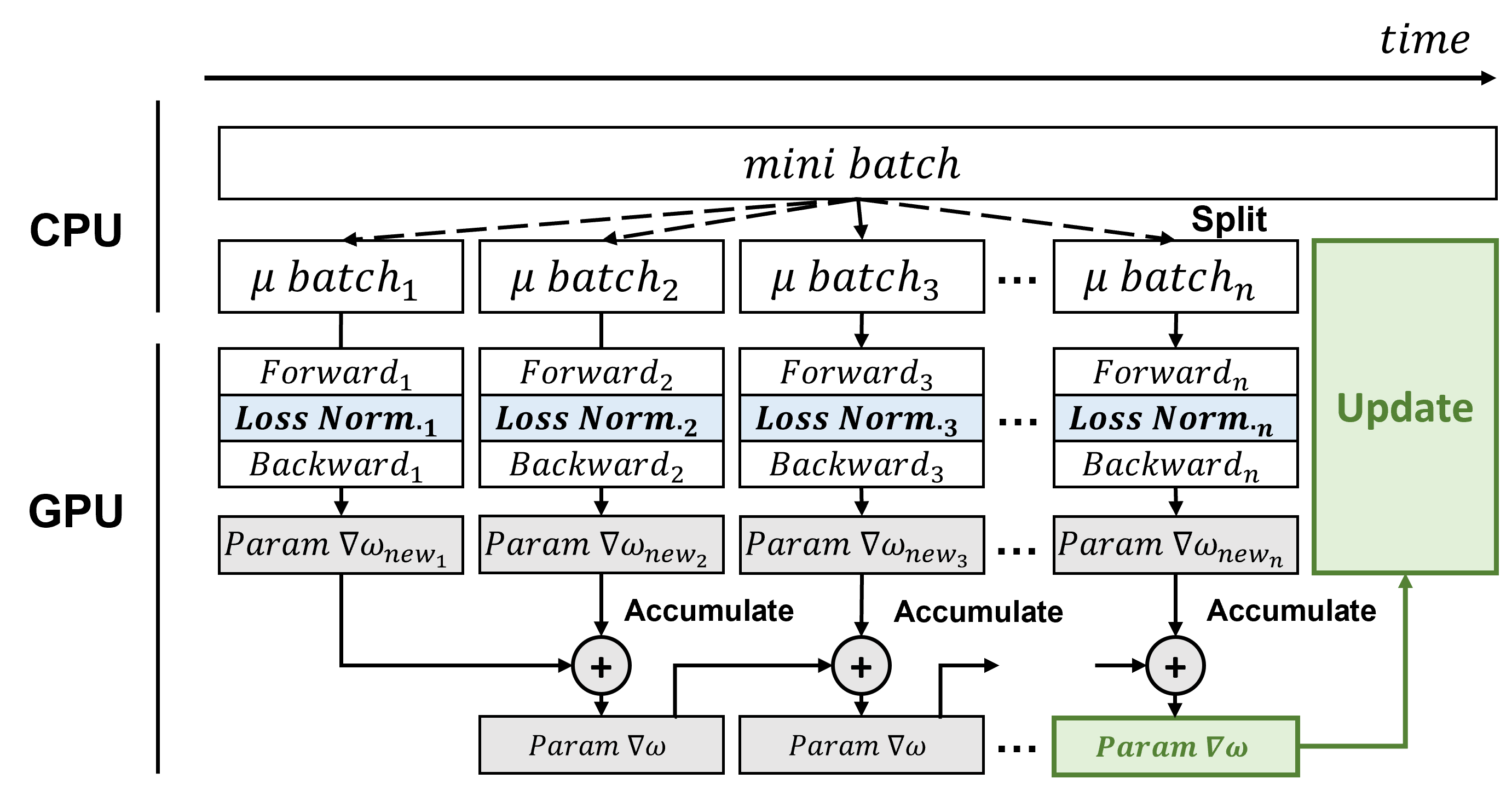
(a) Processing flow over time

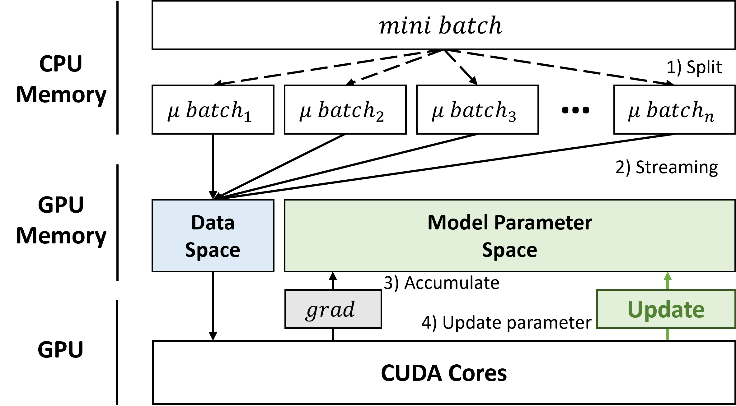
(b) A system perspective of MBS

Figure 1: Overview of Micro-Batch Streaming (MBS)

3.1 Stream-based Pipeline

The stream-based pipeline is a pipeline method that splits the data and streams them sequentially to target devices. Usually, the batch data is pre-loaded into the main memory before being loaded and trained in the GPU. Because of the limited size of the GPU’s memory, it may not be possible to load a large batch of data onto the GPU memory for training. The stream-based pipeline used in the Micro-Batch Streaming (MBS) splits a large batch of data into smaller batches that can be allocated to the remaining GPU memory after the learning model is loaded. Therefore, the MBS enables the training of a DNN model to use a larger mini-batch that exceeds the remaining memory space after the loading of the learning model by training micro batches that fit into the remaining memory streamed from the CPU.

3.2 Micro-Batch

In MBS, the micro-batch ($\mu$-batch) in [8] is extended and is defined as; 1) a unit of streaming to the target device, and 2) a unit of computing on the target device. The first definition presents the splitting of the input mini-batch into micro batches that can fit onto the remaining memory space and streaming them sequentially to the target device. The second statement describes the unit size that target device uses to train the neural network. The formulation of the micro-batch can be expressed as follows.

$$mini\,batch=\bigcup_{i\in S_{\mu}}\mu\,batch_{i}$$ (1)

$$\mu\,batch_{i}\subset mini\,batch\;(i\in S_{\mu})\\ \vspace{0.06cm}$$ (2)

$$\mu\,batch_{size}\leq mini\,batch_{size}$$ (3)

where $S_{\mu}$ in equation 1 and 2 is the set of micro-batches for that certain mini-batch. The micro-batch effectively removes the dependency between the mini-batch size and the target device’s memory capacity. While MBS is using micro-batch for training, this information is accrued such that the model can be trained as if using a large mini-batch size.

3.3 MBS Process

Figure 1 and 2 show the overview of the process of MBS between CPU and GPU. The input mini-batch is split into micro-batches in the CPU, and these micro-batches are sequentially streamed by the CPU to the GPU for computation. When the learning model starts to train, the GPU memory is split into two domains (shown in figure 2); one is the model parameter space where model parameters and gradients reside, and the other is the data space where tensorized input batch and intermediate outcomes are populated. The data in the model parameter space is used to determine the updates of the deep learning model’s parameters. The intermediate outcomes that are computed by the forward pass of the model and in the data space are used to calculate the gradients in the following processes.

The training process using the MBS is as follows (figure 2). First, MBS loads the mini-batch dataset to the CPU memory space and then splits the mini-batch into $n$ micro-batches in preparation to stream to the GPU (❶). Then, the micro-batches are streamed sequentially to the GPU and the GPU starts to train the model using each micro-batch (❷). The GPU executes the forward and backward steps and stores the gradient in the model parameter space (❸). Only when all the micro-batches in the mini-batch are used for training, the model parameters are updated. The gradients computed by the forward and backward propagation are accumulated until all micro-batch is processed (❹). When the final micro-batch is completed, MBS updates the model parameters using the accumulated gradient, similar to the gradient computed by the mini-batch (❺). Therefore, it is as though the model’s parameters are updated using the mini-batch, while the gradients are computed from micro-batches.

The accumulated gradient is computed using the gradient accumulation method that adds the earlier gradients and current gradient until a update. This results in the accumulated gradient being larger than the gradient computed by using a mini-batch. This is because the training process of deep learning model using the MBS and using the mini-batch is different. Thus, the resulting performance can be different. This paper introduces a loss normalization method that normalizes the loss calculated using MBS by a loss function at every micro-batch iteration. The necessity and appropriateness of loss normalization is described in detail in the next section. In MBS, the loss normalization method is used for the automatic update of gradients and MBS waits until all micro-batches, split from a mini-batch, are completed before the update. The timing of the update will seem to be the same as an update after a mini-batch is completed.

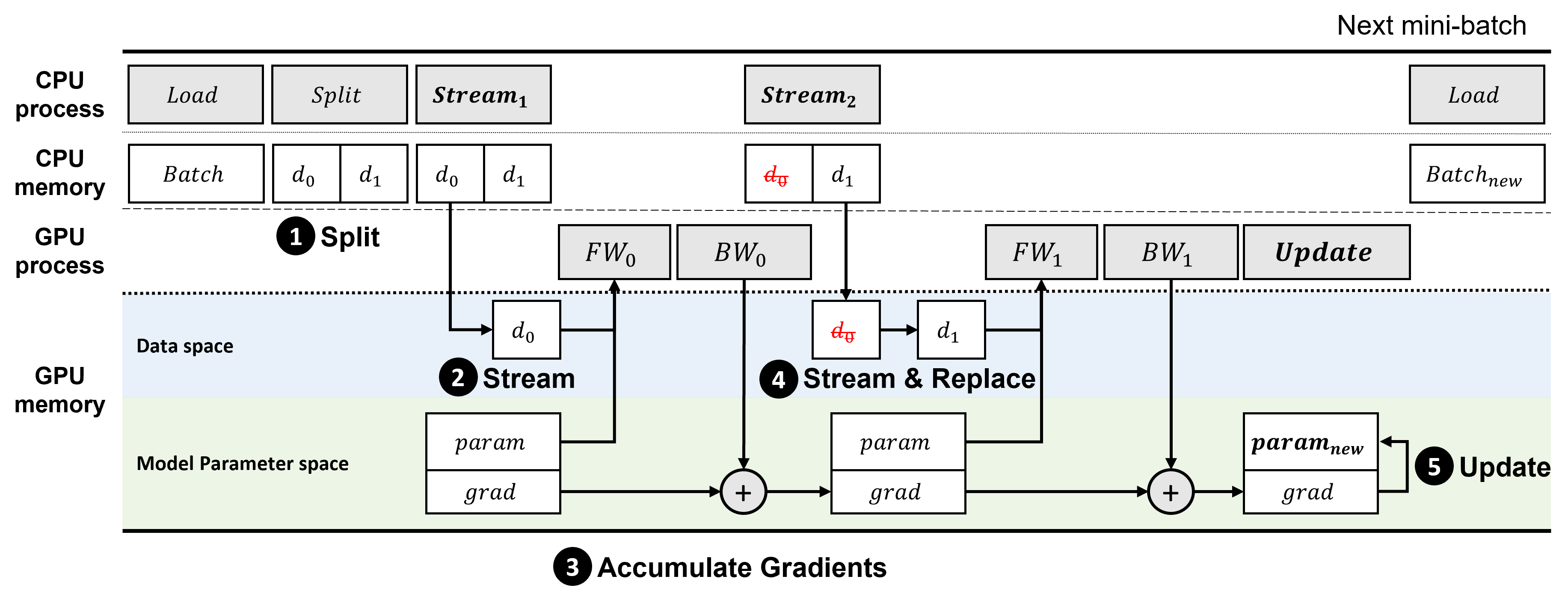
Figure 2: The training process using MBS.

3.4 Loss Normalization

Stochastic Gradient Descent (SGD) [10] is one of the widely used method for deep learning. SGD computes the loss from the difference between outputs computed from the forward pass in the model and targets. MBS adopted the gradient accumulation to derive the gradient of the mini-batch using gradients calculated and accumulated from using micro-batches. If loss accumulation is performed without loss normalization in the micro-batch loss calculation, loss calculated at every micro-batch unit will be accumulated, leading to a different loss calculation compared to the loss calculated without MBS. This section defines the problem of gradient accumulation in the case of training using MBS and proves the necessity and appropriateness of the loss normalization method introduced in this paper.

Gradient accumulation calculates the sum of the previous gradient and the current gradient until updated ($\nabla\omega_{accum}=\sum_{i=0}^{n}\nabla\omega_{i}$). The formulation of loss ($\mathcal{L}_{B}$) and gradient ($\nabla\omega_{B}$) for a mini-batch can be expressed as follows:

$$\mathcal{L}_{B}={\frac{1}{N_{B}}}\sum_{i=1}^{N_{B}}\mathcal{L}(output_{i},target_{i})={\frac{1}{N_{B}}}\sum_{i=1}^{N_{B}}\mathcal{L}_{i}$$ (4)

$$\nabla\omega_{B}=\partial(\mathcal{L}_{B})=\partial({\frac{1}{N_{B}}}\sum_{i=1}^{N_{B}}\mathcal{L}_{i})$$ (5)

$$N_{B}=N_{S_{\mu}}\times N_{\mu}$$ (6)

where $\mathcal{L}_{i}$ is loss that is calculated between output and target for the $i$-th batch in one mini-batch, $N_{S_{\mu}}$ is the size of set of micro-batches in a mini-batch, $N_{\mu}$ is the size of the micro-batch, and $N_{B}$ is the size of the mini-batch. The formulation of loss between a mini-batch and micro-batches can be defined as follows (equation 7 and 8):

$$\sum_{i=1}^{N_{B}}\mathcal{L}_{i} =\sum_{j=1}^{N_{S_{\mu}}}\sum_{k=1}^{N_{\mu}}\mathcal{L}_{j,k}$$ (7)

$$\frac{1}{{N_{B}}}\sum_{i=1}^{N_{B}}\mathcal{L}_{i} =\frac{1}{N_{S_{\mu}}\cdot N_{\mu}}\sum_{j=1}^{N_{S_{\mu}}}\sum_{k=1}^{N_{\mu}}\mathcal{L}_{j,k}$$ (8)

The relationship of the gradient between a mini-batch and micro-batches can be expressed as follows:

$$\nabla\omega_{B} =\partial({\frac{1}{N_{B}}}\sum_{i=1}^{N_{B}}\mathcal{L}_{i})$$ (9)

$$=\partial({\frac{1}{N_{S_{\mu}}\cdot N_{\mu}}}\sum_{j=1}^{N_{S_{\mu}}}\sum_{k=1}^{N_{\mu}}\mathcal{L}_{j,k})$$ (10)

$$=\partial({\frac{1}{N_{S_{\mu}}}}\sum_{k=1}^{N_{S_{\mu}}}({\frac{1}{N_{\mu}}}\sum_{j=1}^{N_{\mu}}\mathcal{L}_{j})_{k})$$ (11)

$$=\partial({\frac{1}{N_{S_{\mu}}}}\sum_{k=1}^{N_{S_{\mu}}}(\mathcal{L}_{\mu})_{k})$$ (12)

where $\nabla\omega_{B}$ is the gradient of one mini-batch, and $\mathcal{L}_{\mu}$ is the loss of one micro-batch. The accumulated gradient ($\nabla\omega_{accum}$) can be expressed as follows:

$$\nabla\omega_{accum}=\sum_{k=1}^{N_{S_{\mu}}}(\nabla\omega_{\mu})_{k}=\sum_{k=1}^{N_{S_{\mu}}}\partial(\mathcal{L}_{\mu})_{k}=\partial(\sum_{k=1}^{N_{S_{\mu}}}(\mathcal{L}_{\mu})_{k})$$ (13)

The above equations (from equation 12 to equation 13) prove that the accumulated gradient is not equal to the gradient of a mini-batch. This means that there is a need for a method to normalize the gradients of a mini-batch that uses the MBS.

To calculate the gradient of mini-batch, we considered two normalization methods; one is normalizing the accumulated gradient for each layer, the other is normalizing loss computed by the loss function. These two methods provide the same effect of normalizing the gradient. However, the former method uses a complex algorithm to normalize the accumulated gradients for each layer, and it will cause heavy overhead at run-time. The latter method does not have a heavy overhead at run-time because it is a simple method that normalizes the accumulated loss (equation 14). Therefore, the latter method to normalize the gradient is used for MBS because this method provides the similar effect of normalizing and is very simple.

$$\mathcal{L}_{norm_{j}} =\frac{1}{N_{S_{\mu}}}\times\mathcal{L}_{\mu_{j}}$$ (14)

$$\sum_{j=1}^{N_{S_{\mu}}}\partial(\mathcal{L}_{norm_{j})} =\sum_{j=1}^{N_{S_{\mu}}}\partial(\frac{1}{N_{S_{\mu}}}\times\mathcal{L}_{\mu_{j}})$$ (15)

$$=\sum_{j=1}^{N_{S_{\mu}}}\partial(\frac{1}{N_{S_{\mu}}}\times\frac{1}{N_{\mu}}\sum_{k=1}^{N_{\mu}}\mathcal{L}_{j,k})$$ (16)

$$=\partial(\frac{1}{N_{S_{\mu}}\cdot N_{\mu}}\sum_{j=1}^{N_{S_{\mu}}}\sum_{k=1}^{N_{\mu}}\mathcal{L}_{j,k})$$ (17)

The above equations (from equation 15 to equation 17) prove that the loss normalization provides the same calculation compared to equation 10. The loss normalization algorithm dynamically determines the normalizing factor and normalizes the loss considering the current input mini-batch size because the mini-batch size is not guaranteed to be uniform for all iterations (shown in Algorithm 1).

0:  The size of micro-batch $N_{\mu}$, a mini-batch $B$

1:  Count the size of mini-batch $N_{B}$ from $B$

2:  if  $N_{B}<N_{\mu}$  then

3:     $N_{\mu}\leftarrow N_{B}$

4:  end if

5:  $N_{S_{\mu}}$ $\leftarrow$ Round-up($N_{B}$ / $N_{\mu}$)

6:  List of micro-batches ($\mu$) $\leftarrow$ Split(B, $N_{\mu}$)

7:  $i$ $\leftarrow$ 0

8:  while  $i<N_{S_{\mu}}$  do

9:     Forward-propagation using micro-batch ($\mu$_i)

10:     $\mathcal{L}_{\mu_{i}}\leftarrow\mathcal{L}(output_{i},target_{i})$

11:     $\mathcal{L}_{norm}\leftarrow\mathcal{L}_{\mu_{i}}/N_{S_{\mu}}$

12:     Backward-propagation and accumulate gradients using $\mathcal{L}_{norm}$

13:     $i\leftarrow i+1$

14:  end while

15:  Update the DNN model parameters using accumulated gradients by optimizer

Algorithm 1 Loss Normalization Algorithm

4 Evaluation

4.1 Overview

Experiments show that MBS is an efficient method to train deep learning models with a large batch regardless of models, datasets, data size and capacity of GPU memory in limited memory environments. The loss normalization method presented in this paper is used and it seems to be a good method that maintains performance when training using MBS.

4.2 Experimental Setup

4.2.1 Systems

The experiments are run on a system consisting of GeForce RTX 3090 GPU with 24GB GDDR6 memory, intel i7 3.7GHz 6-Core processor, and 64GB main memory. MBS was implemented by using PyTorch version 1.10.2 and CUDA version 11.3.

4.2.2 Models

We evaluate MBS performance with three different types of model architectures. For image classification tasks, two ResNet models [11] (ResNet-50 and ResNet-101) and the AmoebaNet [12] model that uses the architecture search algorithm are used for comparison. Specifically, the AmoebaNet-D model that is used consists of 6 layers and 190 filters and is implemented in [8]. For semantic segmentation tasks, the U-Net [13] model, commonly used in many research, is used for testing MBS. The batch normalization layers, which compute the statistics along the input mini-batch dimension, are included in the experiment models.

4.2.3 Datasets

To evaluate the performance of the proposed MBS, two datasets are used that consist of large image size data. One is the Flower-102 dataset [14] which includes 8,189 color images in 102 classes, where each class consists of between 40 and 258 images, for image classification tasks. The image size of Flower-102 dataset varies, ranging from 500 $\times$ 500 up to 1168 $\times$ 500. The other is the Carvana dataset which consists of both color images and binary images of 5,088 1918$\times$1280 image resolution for semantic segmentation tasks.

The original image size is not appropriate for comparison between the learning models that use or not use MBS. Because if the image size is too large, the baseline models that do not use MBS will fail even after 2 mini-batch size because of the memory limitations. Thus, the image size of the given datasets are resized. The image size of Flower-102 dataset was fixed to 224 $\times$ 224, which is widely used image size is other research such as [8, 15, 16] in image classification tasks, for the ResNet models. For the AmoebaNet-D model, the image size of Flower-102 dataset was fixed at 416 $\times$ 416 image size which is used in [8]². The image size of Carvana dataset was fixed at 384 $\times$ 384 as used in [17] with the method of random crop from a resized 959 $\times$ 640 image, which is a method to crop the given image at random location, for U-Net models.

4.2.4 Methods

ResNet-50 and ResNet-101 models are both trained using the same cross-entropy loss function and the SGD optimizer with parameters set to 0.01 learning rate, 0.9 momentum, and 0.0005 decay. AmoebaNet-D model is trained using the cross-entropy loss function, SGD optimizer with parameters set to 0.1 learning rate, 0.9 momentum, and 0.0001 decay. AmoebaNet-D uses a learning rate scheduler that reduces the learning rate linearly during training.

U-Net model is trained using binary cross-entropy (BCE) loss with dice coefficient (DC), Adam optimizer with parameters set to 0.01 learning rate, 0.0005 decay, and without learning rate scheduler. The dice coefficient [18] is one of widely used metrics to measure the similarity between images for semantic segmentation, and represents the value between 0 and 1. The dice coefficient can be expressed as follows:

$$DC=\frac{2|A\cap B|}{|A|+|B|}$$ (18)

where $A$ means the ground-truth image, and $B$ means the binary image predicted/computed by the learning model. And then, we use the dice coefficient as loss function and combine it with binary cross entropy loss. The loss of dice coefficient($Loss_{dc}$) and the combined loss($Loss_{total}$) can be expressed as follows:

$$\mathcal{L}_{dc}=1-DC=1-\frac{2|A\cap B|}{|A|+|B|}$$ (19)

$$\mathcal{L}_{total}=\mathcal{L}_{bce}+\mathcal{L}_{dc}$$ (20)

Note that MBS uses the default training algorithm in PyTorch [19] to evaluate performance and pre-trained models are not used in the experiments.

4.3 Experimental Results

4.3.1 Training Performance

The training performance of MBS in all models is shown using the size of mini-batch and micro-batch shown in table 2. The size of mini-batch is determined to be the maximum size that can be computed on the GPU and the size of micro-batch for MBS is determined to be half the size of mini-batch for comparison.

Table 2: Initial size of mini-batch and micro-batch for different models.

Tasks	Model	mini-batch	$\mu$-batch
Classification	ResNet-50	16	8
	ResNet-101	8	4
	AmoebaNet-D	32	16
Segmentation	U-Net	16	8

Figure 3 shows the overall performance of training between models with and without MBS for image classsification tasks. The loss and accuracy at each epoch are very similar for all methods with or without MBS. This shows that the model using MBS is trained similarly to the model not using MBS and this means that the loss normalization method used in this paper is appropriate. This also shows that the MBS method does not affect the model performance during training like other hyper-parameter such as (mini) batch size that is used as the unit of computation/streaming on GPU. Maximum accuracy for each model is shown in Table 4.

Figure 3: Performance for each model in image classification models.

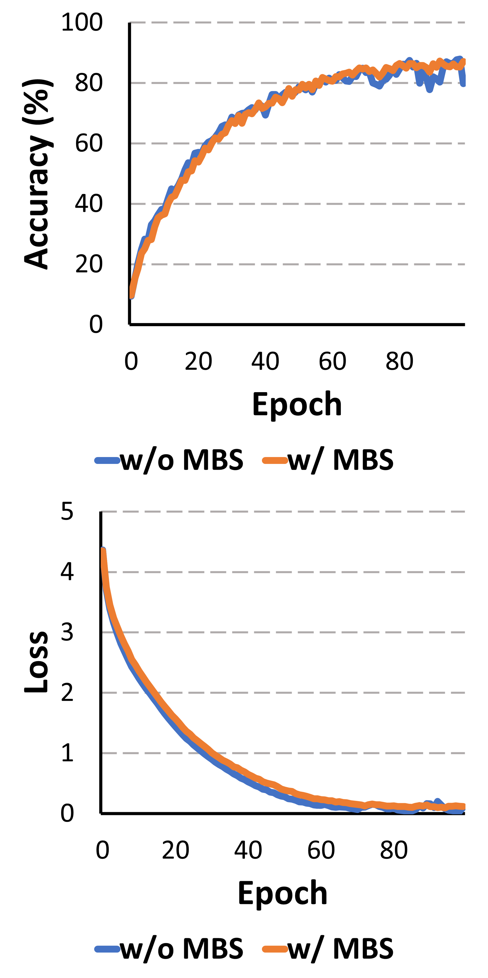
(a) ResNet-50

(b) ResNet-101

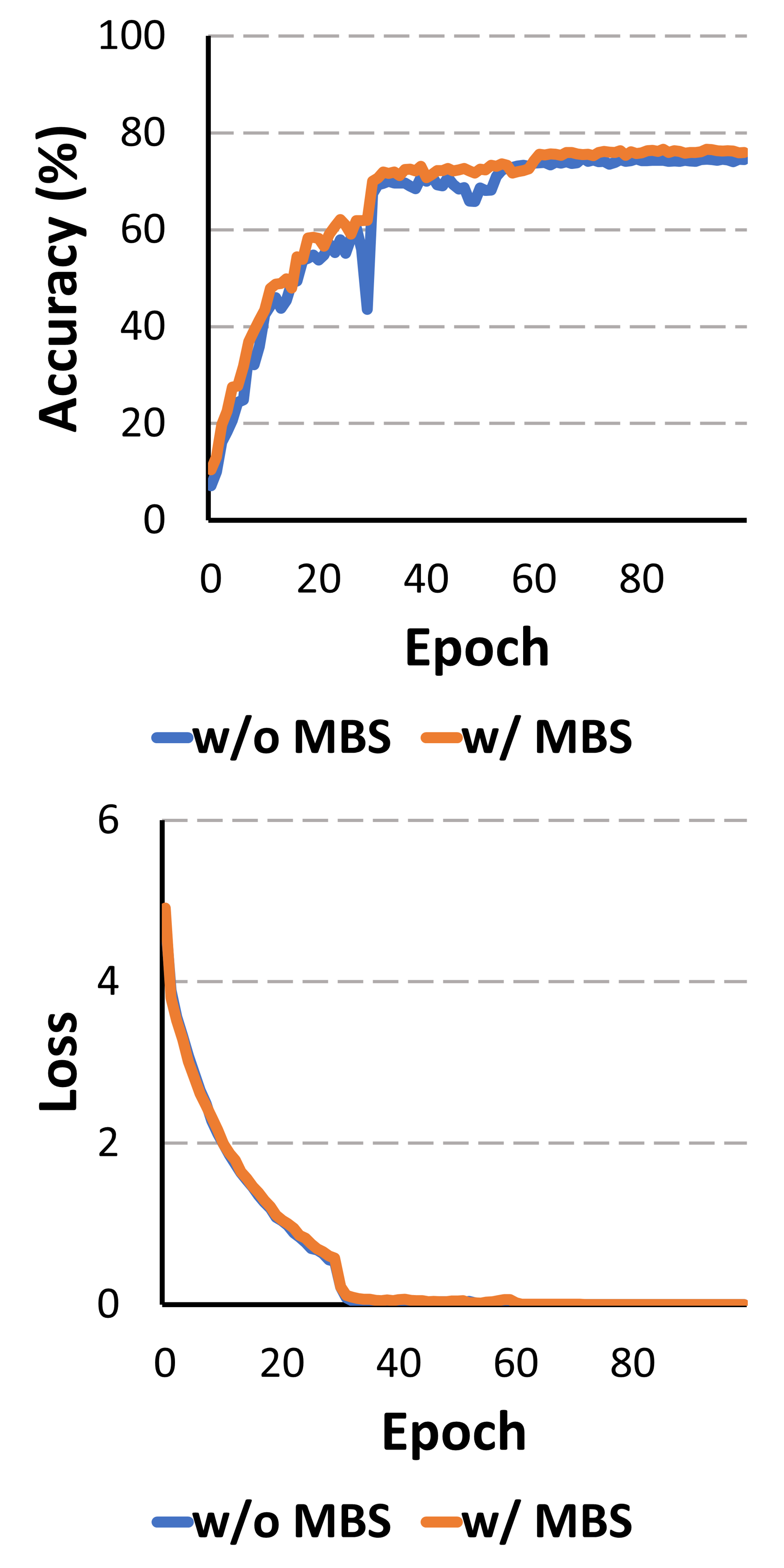
(c) AmoebaNet-D

To evaluate the results of U-Net, we use a metric called intersection over union (IoU) [20], which is one of metrics to evaluate performance in semantic segmentation tasks and shows the degree of the area of overlap between the predicted image and the ground-truth image. The result in table 3 shows the performance of training between with and without MBS for U-Net. The initial experiment shows that the performance is comparable.

Table 3: Performance for a semantic segmentation model.

Metrics	w/o MBS	w/ MBS
IoU (%)	95.48 $\pm$0.13	95.45 $\pm$0.26

Table 4: Accuracy and training time of larger batch sizes than the remaining GPU memory for image classification tasks

Model	Batch size	$\mu$-batch size	Accuracy (%)		Training time (sec)
			w/o MBS	w/ MBS	w/o MBS	w/ MBS
ResNet-50	16	8	87.16 $\pm$0.33	87.04 $\pm$1.04	226.8 $\pm$0.01	233.0 $\pm$0.01
	32	16	Failed	86.51 $\pm$2.14	Failed	229.4 $\pm$0.02
	64	16	Failed	88.96 $\pm$0.41	Failed	227.4 $\pm$0.02
	128	16	Failed	89.61 $\pm$0.14	Failed	227.5 $\pm$0.02
	256	16	Failed	88.18 $\pm$0.64	Failed	229.4 $\pm$0.02
	512	16	Failed	85.95 $\pm$0.11	Failed	232.6 $\pm$0.03
	1024	16	Failed	77.63 $\pm$0.86	Failed	238.2 $\pm$0.02
ResNet-101	8	4	85.82 $\pm$1.84	83.54 $\pm$2.51	385.5 $\pm$0.02	405.0 $\pm$0.01
	16	8	Failed	86.35 $\pm$2.19	Failed	381.9 $\pm$0.01
	32	8	Failed	86.59 $\pm$1.70	Failed	381.3 $\pm$0.01
	64	8	Failed	85.94 $\pm$1.02	Failed	381.5 $\pm$0.01
	128	8	Failed	88.14 $\pm$0.42	Failed	382.1 $\pm$0.01
	256	8	Failed	87.90 $\pm$0.28	Failed	383.8 $\pm$0.02
	512	8	Failed	82.72 $\pm$0.67	Failed	386.4 $\pm$0.03
	1024	8	Failed	75.14 $\pm$0.67	Failed	392.8 $\pm$0.02
AmoebaNet-D	32	16	74.51 $\pm$0.67	75.92 $\pm$1.59	95.2 $\pm$0.01	100.1 $\pm$0.22
	64	32	Failed	73.78 $\pm$0.43	Failed	95.7 $\pm$0.04
	128	32	Failed	73.23 $\pm$1.59	Failed	96.4 $\pm$0.02
	256	32	Failed	75.80 $\pm$0.17	Failed	98.9 $\pm$0.17
	512	32	Failed	74.69 $\pm$0.49	Failed	103.9 $\pm$0.19
	1024	32	Failed	72.49 $\pm$1.10	Failed	111.1 $\pm$0.06

Table 5: IoU and training time of larger batch sizes than the remaining GPU memory for semantic segmentation task

Model	Batch size	$\mu$-batch size	IoU (%)		Training time (sec)
			w/o MBS	w/ MBS	w/o MBS	w/ MBS
U-Net	16	8	95.48 $\pm$0.13	95.45 $\pm$0.26	180.7 $\pm$0.18	183.2 $\pm$0.20
	32	16	Failed	96.13 $\pm$0.13	Failed	180.5 $\pm$0.24
	64	16	Failed	96.83 $\pm$0.12	Failed	182.8 $\pm$0.28
	128	16	Failed	97.51 $\pm$0.06	Failed	187.0 $\pm$0.24
	256	16	Failed	96.96 $\pm$0.16	Failed	194.2 $\pm$0.21
	512	16	Failed	94.18 $\pm$0.44	Failed	207.3 $\pm$0.21
	1024	16	Failed	94.18 $\pm$0.44	Failed	228.0 $\pm$0.07

4.3.2 Maximum Batch Size

If MBS is used, one can compute the entire batch by streaming small batches regardless of the type of models, datasets, entire batch size and the capacity of a device memory, if necessary. Experimental results are shown in table 4 and 5. Three different random seeds are used for the experimental results, and the mean and standard deviation of maximum accuracy/IoU for each random seed are calculated. The size of mini-batch starts from the maximum size that can be computed on the GPU (without using MBS). As the mini-batch sizes of each of the learning models are increased, the model that uses MBS can continue to train while previous methods that does not use MBS fail because of limited memory size.

ResNet-50 model uses 7 different mini-batch sizes, ResNet-101 model uses 8 different mini-batch sizes, and AmoebaNet-D model uses 6 different mini-batch sizes to evaluate MBS performance in this experiment. The U-Net model use 7 different mini-batch sizes to evaluate MBS performance, and the result shows the maximum IoU value for each mini-batch sizes and micro-batch sizes in table 5. The micro-batch size is experimentally determined; 1) the half of mini-batch size in the smallest mini-batch, 2) the maximum size that can compute on GPU in other large mini-batches.

Table 4 and 5 shows the accuracy or IoU for each mini-batch and micro-batch. Without MBS, all models fail to train models using a large mini-batch because the capacity of GPU memory is not enough to allocate a large mini-batch. When using MBS, all models are trained using a large mini-batch up to a given maximum size on the same GPU. Compared to models without MBS, deep learning models are trained using 64$\times$ larger mini-batch in ResNet-50 model, 128$\times$ larger mini-batch in ResNet-101 model, and 32$\times$ larger mini-batch in AmoebaNet-D model. Moreover, the U-Net can train using 64$\times$ larger mini-batch sizes compared to the same model without MBS. Although the input data size is 3.45$\times$ larger for AmoebaNet-D model and 2.94$\times$ larger for U-Net model than the input data size for ResNet models, AmoebaNet-D and U-Net models can increase the size of mini-batch up to the given maximum size when using MBS. Theoretically, MBS allows the increase of the mini-batch size up to the total size of the dataset, if necessary.

It is observed that MBS can be used to determine or find the optimal (mini) batch size for each model. Determining the optimal batch size for a deep learning model will affect that model’s performance. When using MBS, ResNet-50 model achieved 2.44% higher accuracy in 128 mini-batch sizes, and ResNet-101 model achieved 2.32% higher accuracy in 128 mini-batche sizes and it is shown in table 4. Although AmeobaNet-D model using MBS shows 1.41% higher accuracy in 32 mini-batch size, comparable performance of 1.29% higher is shown in 256 mini-batch size. The U-Net model shows higher percentage of IoU score between 32 and 256 mini-batch sizes as shown in table 5. The U-Net model achieved 97.51% the highest percentage of IoU score in 128 mini-batch size, and it is 2.03% higher compared to the model without MBS. Previously, research on deep learning models had difficulty searching for the optimal batch size and train using a large batch, due to the limitation of hardware resource such as the GPU memory capacity and had to consider multiple GPU(s) and/or virtual memory for GPUs. MBS allows large mini-batch size even on a single memory limited device.

4.3.3 Training time

Deep learning models using MBS process multiple back-propagations for multiple micro-batches until updated for one mini-batch. This is because MBS splits one mini-batch into several micro-batches and streams micro-batches to GPU sequentially. To update the model parameters for one mini-batch, MBS process multiple back-propagations for micro-batches. This process will cause the overhead for training time. Table 4 and 5 show the results for average training time for one epoch between with and without MBS. Deep learning models without MBS show almost less training time compared to models with MBS except for the ResNet-101 model. The results show that average training time will increase as the mini-batch size is increased. This is because the overhead of loading images from secondary memory to CPU memory affects training time more than MBS process overhead. On the other hand, the overhead of training time is relatively small when using the mini-batch size that shows the best performance. The ResNet-50 model shows 1.1% and 0.3% training overhead in 32 and 128 mini-batch size, AmoebaNet-D model shows 5.1% and 4.0% training overhead in 32 and 256 mini-batch size, and U-Net models shows 3.5% training overhead in 128 mini-batch size.

5 Conclusion

This paper proposes and introduces Micro-Batch Streaming (MBS), an efficient and novel method based on stream-based pipeline computation to allow deep learning models to train with large batches on limited memory size devices. The loss normalization scheme provides a method to maintain the performance while using a micro batch size that is a subset of a larger mini-batch size and that fits into the remaining memory space after the upload of the learning model. All this without increasing the memory and without using multiple GPUs. MBS allows the training of a learning model to use a large mini-batch size up to the maximum number of training samples. MBS is applied to classification models and a semantic segmentation model, showed overall comparable results, some results show higher performance, and allowed larger mini-batch sizes than previous methods.

References

- [1] Chao Peng, Tete Xiao, Zeming Li, Yuning Jiang, Xiangyu Zhang, Kai Jia, Gang Yu, and Jian Sun. Megdet: A large mini-batch object detector. In Proceedings of the IEEE conference on Computer Vision and Pattern Recognition, pages 6181–6189, 2018.
- [2] Qirong Ho, James Cipar, Henggang Cui, Seunghak Lee, Jin Kyu Kim, Phillip B Gibbons, Garth A Gibson, Greg Ganger, and Eric P Xing. More effective distributed ml via a stale synchronous parallel parameter server. Advances in neural information processing systems, 26, 2013.
- [3] Zhouyuan Huo, Bin Gu, Heng Huang, et al. Decoupled parallel backpropagation with convergence guarantee. In International Conference on Machine Learning, pages 2098–2106. PMLR, 2018.
- [4] Zhihao Jia, Matei Zaharia, and Alex Aiken. Beyond data and model parallelism for deep neural networks. Proceedings of Machine Learning and Systems, 1:1–13, 2019.
- [5] Tal Ben-Nun and Torsten Hoefler. Demystifying parallel and distributed deep learning: An in-depth concurrency analysis. ACM Computing Surveys (CSUR), 52(4):1–43, 2019.
- [6] Jeffrey Dean, Greg Corrado, Rajat Monga, Kai Chen, Matthieu Devin, Mark Mao, Marc’aurelio Ranzato, Andrew Senior, Paul Tucker, Ke Yang, et al. Large scale distributed deep networks. Advances in neural information processing systems, 25, 2012.
- [7] Seunghak Lee, Jin Kyu Kim, Xun Zheng, Qirong Ho, Garth A Gibson, and Eric P Xing. On model parallelization and scheduling strategies for distributed machine learning. Advances in neural information processing systems, 27, 2014.
- [8] Yanping Huang, Youlong Cheng, Ankur Bapna, Orhan Firat, Dehao Chen, Mia Chen, HyoukJoong Lee, Jiquan Ngiam, Quoc V Le, Yonghui Wu, et al. Gpipe: Efficient training of giant neural networks using pipeline parallelism. Advances in neural information processing systems, 32, 2019.
- [9] Deepak Narayanan, Aaron Harlap, Amar Phanishayee, Vivek Seshadri, Nikhil R Devanur, Gregory R Ganger, Phillip B Gibbons, and Matei Zaharia. Pipedream: generalized pipeline parallelism for dnn training. In Proceedings of the 27th ACM Symposium on Operating Systems Principles, pages 1–15, 2019.
- [10] Jack Kiefer and Jacob Wolfowitz. Stochastic estimation of the maximum of a regression function. The Annals of Mathematical Statistics, pages 462–466, 1952.
- [11] Kaiming He, Xiangyu Zhang, Shaoqing Ren, and Jian Sun. Deep residual learning for image recognition. In Proceedings of the IEEE conference on computer vision and pattern recognition, pages 770–778, 2016.
- [12] Esteban Real, Alok Aggarwal, Yanping Huang, and Quoc V Le. Regularized evolution for image classifier architecture search. In Proceedings of the aaai conference on artificial intelligence, volume 33, pages 4780–4789, 2019.
- [13] Olaf Ronneberger, Philipp Fischer, and Thomas Brox. U-net: Convolutional networks for biomedical image segmentation. In International Conference on Medical image computing and computer-assisted intervention, pages 234–241. Springer, 2015.
- [14] Maria-Elena Nilsback and Andrew Zisserman. Automated flower classification over a large number of classes. In 2008 Sixth Indian Conference on Computer Vision, Graphics & Image Processing, pages 722–729. IEEE, 2008.
- [15] Aravind Srinivas, Tsung-Yi Lin, Niki Parmar, Jonathon Shlens, Pieter Abbeel, and Ashish Vaswani. Bottleneck transformers for visual recognition. In Proceedings of the IEEE/CVF conference on computer vision and pattern recognition, pages 16519–16529, 2021.
- [16] Kaiming He, Xiangyu Zhang, Shaoqing Ren, and Jian Sun. Deep residual learning for image recognition. In Proceedings of the IEEE conference on computer vision and pattern recognition, pages 770–778, 2016.
- [17] Hu Cao, Yueyue Wang, Joy Chen, Dongsheng Jiang, Xiaopeng Zhang, Qi Tian, and Manning Wang. Swin-unet: Unet-like pure transformer for medical image segmentation. arXiv preprint arXiv:2105.05537, 2021.
- [18] Lee R Dice. Measures of the amount of ecologic association between species. Ecology, 26(3):297–302, 1945.
- [19] Adam Paszke, Sam Gross, Francisco Massa, Adam Lerer, James Bradbury, Gregory Chanan, Trevor Killeen, Zeming Lin, Natalia Gimelshein, Luca Antiga, et al. Pytorch: An imperative style, high-performance deep learning library. Advances in neural information processing systems, 32, 2019.
- [20] Hamid Rezatofighi, Nathan Tsoi, JunYoung Gwak, Amir Sadeghian, Ian Reid, and Silvio Savarese. Generalized intersection over union: A metric and a loss for bounding box regression. In Proceedings of the IEEE/CVF conference on computer vision and pattern recognition, pages 658–666, 2019.
- [21] Yang You, Zhao Zhang, Cho-Jui Hsieh, James Demmel, and Kurt Keutzer. Imagenet training in minutes. In Proceedings of the 47th International Conference on Parallel Processing, pages 1–10, 2018.
- [22] Yang You, Igor Gitman, and Boris Ginsburg. Large batch training of convolutional networks. arXiv preprint arXiv:1708.03888, 2017.
- [23] Martín Abadi, Paul Barham, Jianmin Chen, Zhifeng Chen, Andy Davis, Jeffrey Dean, Matthieu Devin, Sanjay Ghemawat, Geoffrey Irving, Michael Isard, et al. TensorFlow: A system for Large-Scale machine learning. In 12th USENIX symposium on operating systems design and implementation (OSDI 16), pages 265–283, 2016.
- [24] Jia Deng, Wei Dong, Richard Socher, Li-Jia Li, Kai Li, and Li Fei-Fei. Imagenet: A large-scale hierarchical image database. In 2009 IEEE conference on computer vision and pattern recognition, pages 248–255. Ieee, 2009.
- [25] Alex Krizhevsky, Geoffrey Hinton, et al. Learning multiple layers of features from tiny images. 2009.
- [26] Ting Chen, Simon Kornblith, Mohammad Norouzi, and Geoffrey Hinton. A simple framework for contrastive learning of visual representations. In International conference on machine learning, pages 1597–1607. PMLR, 2020.
- [27] Sergey Ioffe and Christian Szegedy. Batch normalization: Accelerating deep network training by reducing internal covariate shift. In International conference on machine learning, pages 448–456. PMLR, 2015.
- [28] Youjie Li, Amar Phanishayee, Derek Murray, and Nam Sung Kim. Doing more with less: Training large dnn models on commodity servers for the masses. In Proceedings of the Workshop on Hot Topics in Operating Systems, pages 119–127, 2021.
- [29] Karen Simonyan and Andrew Zisserman. Very deep convolutional networks for large-scale image recognition. arXiv preprint arXiv:1409.1556, 2014.
- [30] Alex Krizhevsky, Ilya Sutskever, and Geoffrey E Hinton. Imagenet classification with deep convolutional neural networks. Advances in neural information processing systems, 25, 2012.
- [31] Alex Krizhevsky. One weird trick for parallelizing convolutional neural networks. arXiv preprint arXiv:1404.5997, 2014.
- [32] Zhihao Jia, Sina Lin, Charles R Qi, and Alex Aiken. Exploring hidden dimensions in parallelizing convolutional neural networks. In ICML, pages 2279–2288, 2018.
- [33] Priya Goyal, Piotr Dollár, Ross Girshick, Pieter Noordhuis, Lukasz Wesolowski, Aapo Kyrola, Andrew Tulloch, Yangqing Jia, and Kaiming He. Accurate, large minibatch sgd: Training imagenet in 1 hour. arXiv preprint arXiv:1706.02677, 2017.
- [34] Nitish Shirish Keskar, Dheevatsa Mudigere, Jorge Nocedal, Mikhail Smelyanskiy, and Ping Tak Peter Tang. On large-batch training for deep learning: Generalization gap and sharp minima. arXiv preprint arXiv:1609.04836, 2016.
- [35] Mu Li, Tong Zhang, Yuqiang Chen, and Alexander J Smola. Efficient mini-batch training for stochastic optimization. In Proceedings of the 20th ACM SIGKDD international conference on Knowledge discovery and data mining, pages 661–670, 2014.
- [36] Jianmin Chen, Xinghao Pan, Rajat Monga, Samy Bengio, and Rafal Jozefowicz. Revisiting distributed synchronous sgd. arXiv preprint arXiv:1604.00981, 2016.
- [37] Shaoqing Ren, Kaiming He, Ross Girshick, and Jian Sun. Faster r-cnn: Towards real-time object detection with region proposal networks. Advances in neural information processing systems, 28, 2015.
- [38] Priya Goyal, Piotr Dollár, Ross Girshick, Pieter Noordhuis, Lukasz Wesolowski, Aapo Kyrola, Andrew Tulloch, Yangqing Jia, and Kaiming He. Accurate, large minibatch sgd: Training imagenet in 1 hour. arXiv preprint arXiv:1706.02677, 2017.
- [39] Ibrahem Kandel and Mauro Castelli. The effect of batch size on the generalizability of the convolutional neural networks on a histopathology dataset. ICT express, 6(4):312–315, 2020.
- [40] Kaiming He, Georgia Gkioxari, Piotr Dollár, and Ross Girshick. Mask r-cnn. In Proceedings of the IEEE international conference on computer vision, pages 2961–2969, 2017.
- [41] Ross Girshick. Fast r-cnn. In Proceedings of the IEEE international conference on computer vision, pages 1440–1448, 2015.
- [42] Alexey Dosovitskiy, Lucas Beyer, Alexander Kolesnikov, Dirk Weissenborn, Xiaohua Zhai, Thomas Unterthiner, Mostafa Dehghani, Matthias Minderer, Georg Heigold, Sylvain Gelly, et al. An image is worth 16x16 words: Transformers for image recognition at scale. arXiv preprint arXiv:2010.11929, 2020.
- [43] M. Everingham, S. M. A. Eslami, L. Van Gool, C. K. I. Williams, J. Winn, and A. Zisserman. The pascal visual object classes challenge: A retrospective. International Journal of Computer Vision, 111(1):98–136, January 2015.
- [44] Torsten Rohlfing. Image similarity and tissue overlaps as surrogates for image registration accuracy: widely used but unreliable. IEEE transactions on medical imaging, 31(2):153–163, 2011.