Spurious solutions for high order curl problems

Abstract.

We investigate numerical solutions of high order $\operatorname{curl}$ problems with various formulations and finite elements. We show that several classical conforming finite elements lead to spurious solutions, while mixed formulations with finite elements in complexes solve the problems correctly. To explain the numerical results, we clarify the cohomological structures in high order $\operatorname{curl}$ problems by relating the partial differential equations to the Hodge-Laplacian boundary problems of the $\operatorname{grad}\operatorname{curl}$-complexes.

1. Introduction

Spurious solutions usually refer to numerical solutions that converge to a “wrong solution” of partial differential equations (PDEs) or variational problems. Such solutions are dangerous for applications because of the lack of a visible condition (e.g., non-convergence or instability) to tell them from the correct solutions. Spurious solutions of eigenvalue problems are called “the plague” [10] (or, sometimes called the “vector parasites” [29]) since the early days of computational electromagnetism. Several possible reasons were conjectured, for example, violation of the divergence-free condition of the discrete magnetic field (see, e.g., [10, 29, 31] and the references therein). In [29], Sun et al. pointed out that the cause of the problem is not that the precise solenoidal condition fails at the discrete level, but rather a poor discretization of the kernel and range of the operators. In a modern language, this means that the Lagrange finite element fails to fit in a de Rham complex with local finite element spaces. In [29] the authors also discussed a smoother de Rham complex (Stokes complex) on the Powell-Sabin split [18] and showed that the Lagrange vector element avoids spurious solutions on this mesh. This demonstrates that the $C^{0}$ continuity of the Lagrange elements is not an obstacle for eigenvalue problems as long as the underlying complexes exist and appropriate schemes are used (see also [15, 8]).

Spurious solutions also appear in source problems. Solving the vector Laplacian problem using the primal formulation and the Lagrange finite element leads to wrong solutions on an annulus or an L-shape domain [2, 4]. On an annulus domain, the Lagrange elements cannot approximate the harmonic forms due to the lack of a cohomological structure at the discrete level. For the $L$-shape domain, the problem lies in an approximation issue. Since $[H^{1}]^{3}\cap H_{0}(\operatorname{div})$ is a closed subspace in $H(\operatorname{curl})\cap H_{0}(\operatorname{div})$ which in general is not dense in the norm defined by the primal formulation, numerical solutions of the primal formulation with $C^{0}$ elements cannot approximate true solutions with singularity.

For the Maxwell equations, the Nédélec element fixes both issues: on the one hand, it fits into a de Rham sequence with finite element spaces; on the other hand, generally the Nédélec element does not belong to $H^{1}$ [7]. So the finite element scheme converges correctly to singular solutions. The success of the Nédélec element inspired the development of discrete differential forms [9, 20] and the numerical tests on spurious solutions demonstrate the power of the finite element exterior calculus (FEEC) [2, 3, 4].

Recently, high order problems involving the fourth order curl operator $(\operatorname{curl})^{4}$, or its variant, $-\!\operatorname{curl}\!\Delta\!\operatorname{curl}$, draw attention. These operators and PDEs appear in some magnetohydrodynamics and continuum models [12, 14, 24, 26, 28]. It is speculated that spurious solutions may appear in certain discretizations. For example, Zhang and Zhang [36] anticipated that spurious solutions may appear in the 3D quad-curl source problem due to an approximation issue. Delicate finite elements and mixed schemes were constructed for solving high order curl problems (see, e.g., [11, 13, 23, 30, 34, 37]). Nevertheless, to the best of our knowledge, there are no numerical examples and detailed analysis to support the speculation of spurious solutions. For vector Laplacian problems, after showing that the Nédélec element avoids spurious solutions, Bossavit [10] asked the question: can we rigorously prove that spurious modes necessarily appear in certain numerical methods. To the best of our knowledge, this question is still open for both the vector Laplacian and higher order problems.

In this paper, we provide numerical evidence and analysis to show that spurious solutions do exist for high order curl eigenvalue and source problems. This is for several reasons, for example, the lack of the underlying cohomological structures and problems caused by low regularity. We will show that the high order curl problems are naturally related to the $\operatorname{grad}\operatorname{curl}$-complex [5, (46)], and FEEC formulations fix the spurious modes. Specifically, we compare the primal and/or mixed formulations with the $H(\operatorname{grad}\operatorname{curl})$-conforming element [22], the $H^{1}(\operatorname{curl})$-conforming element [16], and the $H^{2}$-conforming (Argyris) element. As we shall see, mixed formulations with finite elements that fit into complexes (c.f.,[21, 22, 27, 33]) lead to correctly convergent solutions, while other combinations may produce spurious solutions.

We also remark that for the biharmonic equation

(1.1) $$\Delta^{2}u=f,$$

another type of spurious solutions may appear [17, 35] if one decomposes the problem and seeks $u,\sigma\in H^{1}$ which solves

(1.2) $$\Delta u=\sigma,\quad\Delta\sigma=f.$$

This is because the solution for (1.1) from a primal weak form is in $H^{2}$, while on domains with corners the solution $u$ from (1.2) may not be in $H^{2}$. Thus mixed formulations based on (1.2) are not equivalent to (1.1) in general. Nevertheless, this is a difference at the continuous level and we do not pursue methods that decouple the high order curl operators, so we will not discuss this issue in this paper.

The rest of the paper will be organized as follows. In Section 2, we show numerical examples of the spurious solutions by comparing various schemes and finite elements. In Section 3, we relate the high order $\operatorname{curl}$ problem to the $\operatorname{grad}\operatorname{rot}$-complex and the Hodge-Laplacian boundary value problem. In Section 4, we show the convergence of the mixed formulations with finite element complexes [22] and analyze the spurious solutions. We provide concluding remarks in Section 5.

2. Finite element discretization for high order curl problems

Unless otherwise specified, in this paper $\Omega$ is a bounded Lipschitz domain in two space dimensions (2D) with unit outward normal vector $\bm{n}$ and unit tangential vector $\bm{\tau}$ on its boundary $\partial\Omega$. We adopt standard notation for Sobolev spaces such as $H^{s}(\Omega)$ with norm $\|\cdot\|_{s}$ and inner product $(\cdot,\cdot)_{s}$. When $s=0$, $H^{0}(\Omega)$ coincides with $L^{2}(\Omega)$, in which case we omit the subscript $0$ in the notation of the norm and the inner product. We use $H_{0}^{s}(\Omega)$ to denote the spaces with vanishing trace.

Define

$$H_{\operatorname{rot}}(\operatorname{grad}\operatorname{rot};\Omega) :=\{\bm{u}\in H(\operatorname{grad}\operatorname{rot};\Omega):\operatorname{rot}\bm{u}=0\mbox{ on }\partial\Omega\},$$

$$X_{\operatorname{rot}} :=H_{\operatorname{rot}}(\operatorname{grad}\operatorname{rot};\Omega)\cap H_{0}(\operatorname{div};\Omega).$$

We consider the following source problem on a simply-connected domain. Denote by $\mathbb{V}$ the space of vectors. For $\bm{f}\in L^{2}(\Omega)\otimes\mathbb{V}$ (tensor product of $L^{2}(\Omega)$ and $\mathbb{V}$), we seek $\bm{u}\in X_{\operatorname{rot}}$ such that

(2.1) $$\begin{split}-\operatorname{curl}\Delta\operatorname{rot}\bm{u}-\operatorname{grad}\operatorname{div}\bm{u}&=\bm{f}\ \text{in}\;\Omega,\end{split}$$

with the boundary conditions

(2.2) $$\Delta\operatorname{rot}\bm{u}=0,\ \operatorname{rot}\bm{u}=0,\text{ and }\bm{u}\cdot\bm{n}=0\ \text{on}\;\partial\Omega.$$

The primal variational formulation is to seek $\bm{u}\in X_{\operatorname{rot}}$ such that

(2.3) $$\begin{split}(\operatorname{grad}\operatorname{rot}\bm{u},\operatorname{grad}\operatorname{rot}\bm{v})+(\operatorname{div}\bm{u},\operatorname{div}\bm{v})&=(\bm{f},\bm{v}),\quad\forall\bm{v}\in X_{\operatorname{rot}}.\end{split}$$

Let $\sigma=-\operatorname{div}\bm{u}$. Then the mixed variational formulation seeks $(\bm{u},\sigma)\in H_{\operatorname{rot}}(\operatorname{grad}\operatorname{rot};\Omega)\times H^{1}(\Omega)$ such that

(2.4) $$\begin{split}(\operatorname{grad}\operatorname{rot}\bm{u},\operatorname{grad}\operatorname{rot}\bm{v})+(\operatorname{grad}\sigma,\bm{v})&=(\bm{f},\bm{v}),\quad\forall\bm{v}\in H_{\operatorname{rot}}(\operatorname{grad}\operatorname{rot};\Omega),\\ (\bm{u},\operatorname{grad}\tau)-(\sigma,\tau)&=0,\quad\forall\tau\in H^{1}(\Omega).\end{split}$$

We also consider the corresponding eigenvalue problem on a general domain. The strong formulation is to seek $(\lambda,\bm{u})\in\mathbb{R}\times X_{\operatorname{rot}}$ such that

(2.5) $$-\operatorname{curl}\Delta\operatorname{rot}\bm{u}-\operatorname{grad}\operatorname{div}\bm{u}=\lambda\bm{u}\quad\text{in}\;\Omega,$$

with the boundary conditions (2.2). The primal variational formulation is to seek $(\lambda;\bm{u})\in\mathbb{R}\times X_{\operatorname{rot}}$ such that

(2.6) $$\begin{split}(\operatorname{grad}\operatorname{rot}\bm{u},\operatorname{grad}\operatorname{rot}\bm{v})+(\operatorname{div}\bm{u},\operatorname{div}\bm{v})&=\lambda(\bm{u},\bm{v}),\ \forall\bm{v}\in X_{\operatorname{rot}}.\end{split}$$

The mixed variational formulation seeks $(\lambda,\bm{u},\sigma)\in\mathbb{R}\times H_{\operatorname{rot}}(\operatorname{grad}\operatorname{rot};\Omega)\times H^{1}(\Omega)$ s.t.

(2.7) $$\begin{split}(\operatorname{grad}\operatorname{rot}\bm{u},\operatorname{grad}\operatorname{rot}\bm{v})+(\operatorname{grad}\sigma,\bm{v})&=\lambda(\bm{u},\bm{v}),\ \forall\bm{v}\in H_{\operatorname{rot}}(\operatorname{grad}\operatorname{rot};\Omega),\\ (\bm{u},\operatorname{grad}\tau)-(\sigma,\tau)&=0,\ \forall\tau\in H^{1}(\Omega).\end{split}$$

We consider four finite element methods (FEMs) to solve the problems (2.1) and (2.5): a primal formulation with the $H^{2}$-conforming Argyris element, a mixed formulation with the $\operatorname{grad}\operatorname{rot}$-conforming element [32], and the mixed and primal formulations with the $H^{1}(\operatorname{rot})$-conforming element [16]. Let $\mathcal{T}_{h}$ be a partition of the domain $\Omega$ consisting of shape regular triangles, and let $\mathcal{V}$ be the set of vertices. We denote by $P_{k}$ the space of polynomials with degree no larger than $k$. For $K\in\mathcal{T}_{h}$, define

$$\mathcal{R}_{k}(K) :=\operatorname{grad}P_{k}(K)\oplus P_{k-1}(K)\bm{x}^{\perp},\ k\geq 4,$$

$$\mathcal{W}_{k}(K):=\Big{\{}\bm{v}\in P_{k}(K) \otimes\mathbb{R}^{2}:\operatorname{rot}\bm{v}\in P_{k-3}(K)\cup\left[P_{k-1}(K)\cap H_{0}^{1}(K)\right]\Big{\}},\ k\geq 4.$$

Remark 2.1.

We can use the Poincaré operator $\mathfrak{p}u=\int_{0}^{1}u(t\bm{x})t\bm{x}^{\perp}\text{d}t$ to construct $\mathcal{W}_{k}(K)$. For example, when $k=4$, $\mathcal{W}_{k}(K)=\operatorname{grad}P_{5}(K)\oplus P_{1}(K)\bm{x}^{\perp}\oplus\{\mathfrak{p}(\lambda_{1}\lambda_{2}\lambda_{3})\}$.

The $H(\operatorname{grad}\operatorname{rot})$- and $H^{1}(\operatorname{rot})$- conforming finite element spaces on the partition $\mathcal{T}_{h}$ are listed as follows:

$$V_{h} =\big{\{}\bm{v}_{h}\in H_{\operatorname{rot}}(\operatorname{grad}\operatorname{rot};\Omega):\ \bm{v}_{h}|_{K}\in\mathcal{R}_{k}(K),\ \forall K\in\mathcal{T}_{h}\big{\}},$$

$$V^{1}_{h}=\big{\{}\bm{v}_{h} \in H^{1}(\operatorname{rot};\Omega)\cap H_{\operatorname{rot}}(\operatorname{grad}\operatorname{rot};\Omega):\ \bm{v}_{h}|_{K}\in\mathcal{W}_{k}(K),\ \forall K\in\mathcal{T}_{h}\big{\}}.$$

Remark 2.2.

We can also choose $V_{h}$ as the other $\operatorname{grad}\operatorname{rot}$-conforming finite element spaces in [22].

We also define the following two finite element spaces for the mixed schemes.

$$S_{h}=\{{w}_{h}\in H^{1}(\Omega):\ w_{h}|_{K}\in P_{k}(K),\ \forall K\in\mathcal{T}_{h}\},$$

$$S_{h}^{1}=\{{w}_{h}\in H^{2}(\Omega):\ w_{h}|_{K}\in P_{k}(K),\ \forall K\in\mathcal{T}_{h},\ w_{h}\in C^{2}(\mathcal{V})\}\text{ for }k\geq 5.$$

The vector-valued $H^{2}$-conforming finite element space is defined as

$$V_{h}^{Arg}=S_{h}^{1}\otimes\mathbb{R}^{2}.$$

Define

$$\mathring{V}^{1}_{h} =\{\bm{v}_{h}\in V_{h}^{1}:\bm{v}_{h}\cdot\bm{n}=0\text{ on }\partial\Omega\},$$

$$\mathring{V}_{h}^{Arg} =\{\bm{v}_{h}\in V_{h}^{Arg}:\bm{v}_{h}\cdot\bm{n}=0\text{ and }\operatorname{rot}\bm{v}_{h}=0\text{ on }\partial\Omega\}.$$

2.1. Source problem

We are in a position to present the four finite element schemes for the problem (2.1).

Scheme 1 (Mixed formulation with the $H(\operatorname{grad}\operatorname{rot})$-conforming element).

Find $(\bm{u}_{h},\sigma_{h})\in V_{h}\times S_{h}$ such that

$$\begin{split}(\operatorname{grad}\operatorname{rot}\bm{u}_{h},\operatorname{grad}\operatorname{rot}\bm{v}_{h})+(\operatorname{grad}\sigma_{h},\bm{v}_{h})&=(\bm{f},\bm{v}_{h}),\ \forall\bm{v}_{h}\in V_{h},\\ (\bm{u}_{h},\operatorname{grad}\tau_{h})-(\sigma_{h},\tau_{h})&=0,\ \forall\tau_{h}\in S_{h}.\end{split}$$

Scheme 2 (Mixed formulation with the $H^{1}(\operatorname{rot})$-conforming element).

Find $(\bm{u}_{h},\sigma_{h})\in V_{h}^{1}\times S_{h}^{1}$ such that

$$\begin{split}(\operatorname{grad}\operatorname{rot}\bm{u}_{h},\operatorname{grad}\operatorname{rot}\bm{v}_{h})+(\operatorname{grad}\sigma_{h},\bm{v}_{h})&=(\bm{f},\bm{v}_{h}),\ \forall\bm{v}_{h}\in V_{h}^{1},\\ (\bm{u}_{h},\operatorname{grad}\tau_{h})-(\sigma_{h},\tau_{h})&=0,\ \forall\tau_{h}\in S_{h}^{1}.\end{split}$$

Scheme 3 (Primal formulation with the $H^{1}(\operatorname{rot})$-conforming element).

Find $\bm{u}_{h}\in\mathring{V}_{h}^{1}$ such that

$$\begin{split}(\operatorname{grad}\operatorname{rot}\bm{u}_{h},\operatorname{grad}\operatorname{rot}\bm{v}_{h})+(\operatorname{div}\bm{u}_{h},\operatorname{div}\bm{v}_{h})&=(\bm{f},\bm{v}_{h}),\quad\forall\bm{v}_{h}\in\mathring{V}_{h}^{1}.\end{split}$$

Scheme 4 (Primal formulation with the $H^{2}$-conforming (Argyris) element).

Find $\bm{u}_{h}\in\mathring{V}_{h}^{Arg}$ such that

$$\begin{split}(\operatorname{grad}\operatorname{rot}\bm{u}_{h},\operatorname{grad}\operatorname{rot}\bm{v}_{h})+(\operatorname{div}\bm{u}_{h},\operatorname{div}\bm{v}_{h})&=(\bm{f},\bm{v}_{h}),\quad\forall\bm{v}_{h}\in\mathring{V}_{h}^{Arg}.\end{split}$$

(a) Scheme 1

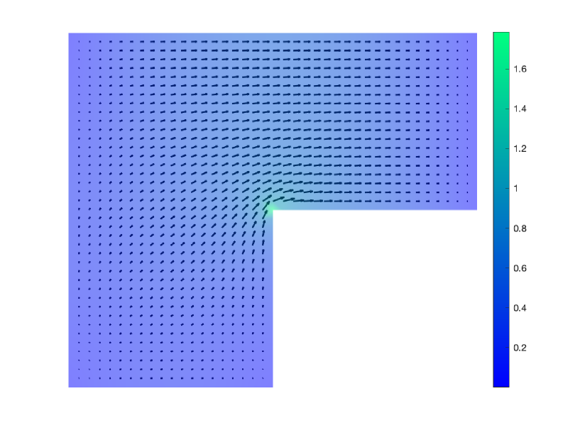
(b) Scheme 2

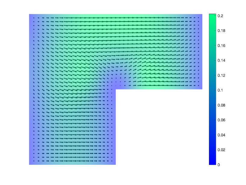
(c) Scheme 3

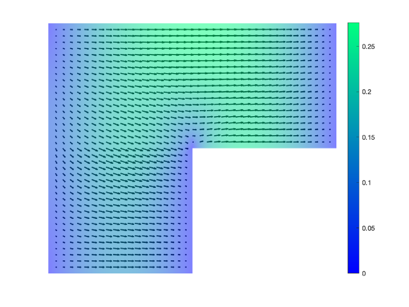
(d) Scheme 4

Figure 2.1. Numerical solutions to the problem (2.1) on an L-shape domain with $\bm{f}=(1,0)^{T}$.

The numerical results for the Hodge-Laplacian source problem (2.1) with $\bm{f}=(1,0)^{\mathrm{T}}$ on an L-shape domain are shown in Figure 2.1. As we see in Figure 2.1, the primal formulation with the Argyris and the $H^{1}(\operatorname{rot})$-conforming finite elements show different solutions compared with the mixed formulations with the $H(\operatorname{grad}\operatorname{rot})$- and $H^{1}(\operatorname{rot})$-conforming elements. In fact, the primal formulation produces spurious solutions, which we will elaborate on in Section 4 by proving the convergence of the mixed formulations and explaining the reason of the spurious solutions.

2.2. Eigenvalue problem

Similar to the source problem, we consider the following four numerical schemes for the problem (2.5).

Scheme 5 (Mixed formulation with the $H(\operatorname{grad}\operatorname{rot})$-conforming element).

Find $(\lambda_{h},\bm{u}_{h},\sigma_{h})\in\mathbb{R}\times V_{h}\times S_{h}$, such that

$$\begin{split}(\operatorname{grad}\operatorname{rot}\bm{u}_{h},\operatorname{grad}\operatorname{rot}\bm{v}_{h})+(\operatorname{grad}\sigma_{h},\bm{v}_{h})&=\lambda_{h}(\bm{u}_{h},\bm{v}_{h}),\ \forall\bm{v}_{h}\in V_{h},\\ (\bm{u}_{h},\operatorname{grad}\tau_{h})-(\sigma_{h},\tau_{h})&=0,\ \forall\tau_{h}\in S_{h}.\end{split}$$

Scheme 6 (Mixed formulation with the $H^{1}(\operatorname{rot})$-conforming element).

Find $(\lambda_{h},\bm{u}_{h},\sigma_{h})\in\mathbb{R}\times V_{h}^{1}\times S_{h}^{1}$, such that

$$\begin{split}(\operatorname{grad}\operatorname{rot}\bm{u}_{h},\operatorname{grad}\operatorname{rot}\bm{v}_{h})+(\operatorname{grad}\sigma_{h},\bm{v}_{h})&=\lambda_{h}(\bm{u}_{h},\bm{v}_{h}),\ \forall\bm{v}_{h}\in V_{h}^{1},\\ (\bm{u}_{h},\operatorname{grad}\tau_{h})-(\sigma_{h},\tau_{h})&=0,\ \forall\tau_{h}\in S_{h}^{1}.\end{split}$$

Scheme 7 (Primal formulation with the $H^{1}(\operatorname{rot})$-conforming element).

Find $(\lambda_{h},\bm{u}_{h})\in\mathbb{R}\times\mathring{V}_{h}^{1}$, such that

$$\begin{split}(\operatorname{grad}\operatorname{rot}\bm{u}_{h},\operatorname{grad}\operatorname{rot}\bm{v}_{h})+(\operatorname{div}\bm{u}_{h},\operatorname{div}\bm{v}_{h})&=\lambda_{h}(\bm{u}_{h},\bm{v}_{h}),\quad\forall\bm{v}_{h}\in\mathring{V}_{h}^{1}.\end{split}$$

Scheme 8 (Primal formulation with the $H^{2}$-conforming (Argyris) element).

Find $(\lambda_{h},\bm{u}_{h})\in\mathbb{R}\times\mathring{V}_{h}^{Arg}$, such that

$$\begin{split}(\operatorname{grad}\operatorname{rot}\bm{u}_{h},\operatorname{grad}\operatorname{rot}\bm{v}_{h})+(\operatorname{div}\bm{u}_{h},\operatorname{div}\bm{v}_{h})&=\lambda_{h}(\bm{u}_{h},\bm{v}_{h}),\quad\forall\bm{v}_{h}\in\mathring{V}_{h}^{Arg}.\end{split}$$

We apply Schemes 5 – 8 to solve the eigenvalue problem (2.5) on three different domains (see Figure 2.2):

• $\Omega_{1}=(0,1)\times(0,1)$.

• $\Omega_{2}=(0,1)\times(0,1)/(1/3,3/4)\times(1/4,2/3)$.

• $\Omega_{3}=(-1,1)\times(-1,1)/(0,1)\times(-1,0)$.

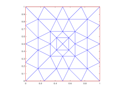
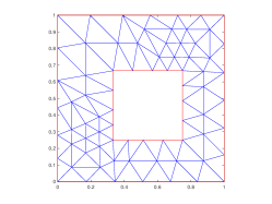
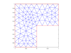
Figure 2.2. Initial meshes (refinement index $n=0$) for $\Omega_{1}$, $\Omega_{2}$, and $\Omega_{3}$

We observe from Table 2.1–2.12 that the four schemes lead to the same numerical eigenvalues on $\Omega_{1}$ and different numerical eigenvalues on $\Omega_{2}$ and $\Omega_{3}$. We will prove in Section 4 that Scheme 5 produces correctly convergent numerical eigenvalues on simply-connected domains, which implies that Scheme 7 and Scheme 8 lead to spurious eigenvalues on $\Omega_{3}$.

Table 2.1. Numerical eigenvalues with units $\pi^{2}$ on $\Omega_{1}$ obtained by Scheme 5 with $k=4$ for (2.5)

$n$	$\lambda_{1}$	$\lambda_{2}$	$\lambda_{3}$	$\lambda_{4}$	$\lambda_{5}$	$\lambda_{6}$	$\lambda_{7}$	$\lambda_{8}$
0	1.000000	1.000000	2.000000	4.000001	4.000001	5.000002	5.000002	8.000011
1	1.000000	1.000000	2.000000	4.000000	4.000000	5.000000	5.000000	8.000000
2	1.000000	1.000000	2.000000	4.000000	4.000000	5.000000	5.000000	8.000000

Table 2.2. Numerical eigenvalues with units $\pi^{2}$ on $\Omega_{1}$ obtained by Scheme 6 for (2.5)

$n$	$\lambda_{1}$	$\lambda_{2}$	$\lambda_{3}$	$\lambda_{4}$	$\lambda_{5}$	$\lambda_{6}$	$\lambda_{7}$	$\lambda_{8}$
0	1.000000	1.000000	2.000000	4.000000	4.000000	5.000000	5.000000	8.000001
1	1.000000	1.000000	2.000000	4.000000	4.000000	5.000000	5.000000	8.000000
2	1.000000	1.000000	2.000000	4.000000	4.000000	5.000000	5.000000	8.000000

Table 2.3. Numerical eigenvalues with units $\pi^{2}$ on $\Omega_{1}$ obtained by Scheme 7 for (2.5)

$n$	$\lambda_{1}$	$\lambda_{2}$	$\lambda_{3}$	$\lambda_{4}$	$\lambda_{5}$	$\lambda_{6}$	$\lambda_{7}$	$\lambda_{8}$
0	1.000000	1.000000	2.000000	4.000001	4.000001	5.000004	5.000004	8.000077
1	1.000000	1.000000	2.000000	4.000000	4.000000	5.000000	5.000000	8.000000
2	1.000000	1.000000	2.000000	4.000000	4.000000	5.000000	5.000000	8.000000

Table 2.4. Numerical eigenvalues with units $\pi^{2}$ on $\Omega_{1}$ obtained by Scheme 8 for (2.5)

$n$	$\lambda_{1}$	$\lambda_{2}$	$\lambda_{3}$	$\lambda_{4}$	$\lambda_{5}$	$\lambda_{6}$	$\lambda_{7}$	$\lambda_{8}$
0	1.000000	1.000000	2.000000	4.000000	4.000000	5.000000	5.000000	8.000003
1	1.000000	1.000000	2.000000	4.000000	4.000000	5.000000	5.000000	8.000000
2	1.000000	1.000000	2.000000	4.000000	4.000000	5.000000	5.000000	8.000000

2.3. Eigenvalue problem with different boundary conditions

Denote

$$X=H(\operatorname{grad}\operatorname{rot};\Omega)\cap H_{0}(\operatorname{div};\Omega).$$

In this section, we consider another eigenvalue problem: find $(\lambda,\bm{u})\in\mathbb{R}\times X$, such that

(2.8) $$\begin{split}-\operatorname{curl}\Delta\operatorname{rot}\bm{u}-\operatorname{grad}\operatorname{div}\bm{u}&=\lambda\bm{u}\ \text{in}\;\Omega,\end{split}$$

with the boundary conditions

$$\Delta\operatorname{rot}\bm{u}=0,\ \operatorname{grad}\operatorname{rot}\bm{u}\cdot\bm{n}=0,\text{ and }\bm{u}\cdot\bm{n}=0\ \text{on}\;\partial\Omega.$$

The primal variational formulation is to find $(\lambda,\bm{u})\in\mathbb{R}\times X$ s.t.

(2.9) $$\begin{split}(\operatorname{grad}\operatorname{rot}\bm{u},\operatorname{grad}\operatorname{rot}\bm{v})+(\operatorname{div}\bm{u},\operatorname{div}\bm{v})&=\lambda(\bm{u},\bm{v}),\ \forall\bm{v}\in X.\end{split}$$

The mixed variational formulation is to find $(\lambda,\bm{u},\sigma)\in\mathbb{R}$ $\times H(\operatorname{grad}\operatorname{rot};\Omega)$ $\times H^{1}(\Omega)$ s.t.

(2.10) $$\begin{split}(\operatorname{grad}\operatorname{rot}\bm{u},\operatorname{grad}\operatorname{rot}\bm{v})+(\operatorname{grad}\sigma,\bm{v})&=\lambda(\bm{u},\bm{v}),\ \forall\bm{v}\in H(\operatorname{grad}\operatorname{rot};\Omega),\\ (\bm{u},\operatorname{grad}\tau)-(\sigma,\tau)&=0,\ \forall\tau\in H^{1}(\Omega).\end{split}$$

We consider four numerical schemes similar to Scheme 5–8 but without the boundary condition $\operatorname{rot}\bm{u}_{h}=0$ on the three different domains. Again, we observe that the four schemes lead to different numerical solutions. In particular, from the mixed formulations we obtain one zero eigenvalue on $\Omega_{1}$, $\Omega_{3}$, and two zero eigenvalues on $\Omega_{2}$. On the other hand, other schemes do not produce zero numerical eigenvalues. This difference will also be explained in Section 4.

Table 2.5. Numerical eigenvalues with units $\pi^{2}$ on $\Omega_{2}$ obtained by Scheme 5 with $k=4$ for (2.5)

$n$	$\lambda_{1}$	$\lambda_{2}$	$\lambda_{3}$	$\lambda_{4}$	$\lambda_{5}$	$\lambda_{6}$	$\lambda_{7}$	$\lambda_{8}$
0	0.000000	0.594212	0.595733	1.802009	2.843750	4.460286	4.495899	5.463774
1	0.000000	0.593616	0.595336	1.801970	2.839489	4.458673	4.493247	5.463500
2	0.000000	0.593379	0.595179	1.801959	2.837796	4.458048	4.492200	5.463407

Table 2.6. Numerical eigenvalues with units $\pi^{2}$ on $\Omega_{2}$ obtained by Scheme 6 for (2.5)

$n$	$\lambda_{1}$	$\lambda_{2}$	$\lambda_{3}$	$\lambda_{4}$	$\lambda_{5}$	$\lambda_{6}$	$\lambda_{7}$	$\lambda_{8}$
0	0.000000	0.596944	0.597564	1.802182	2.863546	4.467690	4.508052	5.465057
1	0.000000	0.594698	0.596060	1.802016	2.847332	4.461544	4.498047	5.463929
2	0.000000	0.593808	0.595466	1.801975	2.840909	4.459177	4.494100	5.463565

Table 2.7. Numerical eigenvalues with units $\pi^{2}$ on $\Omega_{2}$ obtained by Scheme 7 for (2.5)

$n$	$\lambda_{1}$	$\lambda_{2}$	$\lambda_{3}$	$\lambda_{4}$	$\lambda_{5}$	$\lambda_{6}$	$\lambda_{7}$	$\lambda_{8}$
0	2.645076	3.202686	3.607223	4.369787	6.145767	7.964110	8.167482	8.213072
1	2.269742	2.874862	3.141026	4.063906	5.846892	7.677691	7.894476	7.971607
2	2.065438	2.689171	2.882076	3.886972	5.659409	7.489803	7.694887	7.864160
3	1.947637	2.579732	2.731537	3.781333	5.542562	7.373284	7.571471	7.797919

Table 2.8. Numerical eigenvalues with units $\pi^{2}$ on $\Omega_{2}$ obtained by Scheme 8 for (2.5)

$n$	$\lambda_{1}$	$\lambda_{2}$	$\lambda_{3}$	$\lambda_{4}$	$\lambda_{5}$	$\lambda_{6}$	$\lambda_{7}$	$\lambda_{8}$
0	2.996956	3.517662	3.946885	4.626899	6.440491	8.154377	8.449486	8.484641
1	2.462447	3.063195	3.349072	4.229950	6.010834	7.860474	8.069506	8.098664
2	2.178163	2.802148	3.008808	3.990078	5.760831	7.614372	7.802093	7.935650
3	2.015498	2.648156	2.808560	3.844587	5.606347	7.451910	7.636857	7.841693

Table 2.9. Numerical eigenvalues with units $\pi^{2}$ on $\Omega_{3}$ obtained by Scheme 5 with $k=4$ for (2.5)

$n$	$\lambda_{1}$	$\lambda_{2}$	$\lambda_{3}$	$\lambda_{4}$	$\lambda_{5}$	$\lambda_{6}$	$\lambda_{7}$	$\lambda_{8}$
0	0.149678	0.358073	1.000000	1.000000	1.153997	1.274383	2.000000	2.172031
1	0.149578	0.358072	1.000000	1.000000	1.153996	1.274062	2.000000	2.171278
2	0.149538	0.358072	1.000000	1.000000	1.153996	1.273934	2.000000	2.170978

Table 2.10. Numerical eigenvalues with units $\pi^{2}$ on $\Omega_{3}$ obtained by Scheme 6 for (2.5)

$n$	$\lambda_{1}$	$\lambda_{2}$	$\lambda_{3}$	$\lambda_{4}$	$\lambda_{5}$	$\lambda_{6}$	$\lambda_{7}$	$\lambda_{8}$
0	0.150209	0.358082	1.000000	1.000000	1.154010	1.276086	2.000000	2.176030
1	0.149788	0.358074	1.000000	1.000000	1.153998	1.274741	2.000000	2.172873
2	0.149621	0.358072	1.000000	1.000000	1.153996	1.274203	2.000000	2.171612

Table 2.11. Numerical eigenvalues with units $\pi^{2}$ on $\Omega_{3}$ obtained by Scheme 7 for (2.5)

$n$	$\lambda_{1}$	$\lambda_{2}$	$\lambda_{3}$	$\lambda_{4}$	$\lambda_{5}$	$\lambda_{6}$	$\lambda_{7}$	$\lambda_{8}$
0	0.416285	0.665296	1.000000	1.000000	1.181067	1.558700	2.000000	2.447851
1	0.393230	0.635841	1.000000	1.000000	1.170019	1.536785	2.000000	2.416211
2	0.379644	0.618841	1.000000	1.000000	1.163726	1.524513	2.000000	2.396893

Table 2.12. Numerical eigenvalues with units $\pi^{2}$ on $\Omega_{3}$ obtained by Scheme 8 for (2.5)

$n$	$\lambda_{1}$	$\lambda_{2}$	$\lambda_{3}$	$\lambda_{4}$	$\lambda_{5}$	$\lambda_{6}$	$\lambda_{7}$	$\lambda_{8}$
0	0.431506	0.667232	1.000000	1.000000	1.185750	1.559335	2.000000	2.471656
1	0.401863	0.638780	1.000000	1.000000	1.173429	1.538747	2.000000	2.429102
2	0.384768	0.621402	1.000000	1.000000	1.165924	1.526300	2.000000	2.404445

Table 2.13. Numerical eigenvalues with units $\pi^{2}$ on $\Omega_{1}$ obtained by Scheme 5 with $k=4$ for (2.8)

$n$	$\lambda_{1}$	$\lambda_{2}$	$\lambda_{3}$	$\lambda_{4}$	$\lambda_{5}$	$\lambda_{6}$	$\lambda_{7}$	$\lambda_{8}$
$0$	0.000000	1.000000	1.000000	2.000000	4.000000	4.000001	5.000002	5.000002
$1$	0.000000	1.000000	1.000000	2.000000	4.000000	4.000000	5.000000	5.000000
$2$	-0.000000	1.000000	1.000000	2.000000	4.000000	4.000000	5.000000	5.000000

Table 2.14. Numerical eigenvalues with units $\pi^{2}$ on $\Omega_{1}$ obtained by Scheme 6 for (2.8)

$n$	$\lambda_{1}$	$\lambda_{2}$	$\lambda_{3}$	$\lambda_{4}$	$\lambda_{5}$	$\lambda_{6}$	$\lambda_{7}$	$\lambda_{8}$
$0$	0.000000	1.000000	1.000000	2.000000	4.000000	4.000000	5.0000001	5.0000001
$1$	0.000000	1.000000	1.000000	2.000000	4.000000	4.000000	5.0000000	5.0000000
$2$	-0.000000	1.000000	1.000000	2.000000	4.000000	4.000000	5.0000000	5.0000000

Table 2.15. Numerical eigenvalues with units $\pi^{2}$ on $\Omega_{1}$ obtained by Scheme 7 for (2.8)

$n$	$\lambda_{1}$	$\lambda_{2}$	$\lambda_{3}$	$\lambda_{4}$	$\lambda_{5}$	$\lambda_{6}$	$\lambda_{7}$	$\lambda_{8}$
0	1.000000	1.000000	2.000000	4.000002	4.000002	5.000004	5.000004	7.762197
1	1.000000	1.000000	2.000000	4.000000	4.000000	5.000000	5.000000	5.940076
2	1.000000	1.000000	2.000000	4.000000	4.000000	4.833375	5.000000	5.000000
3	1.000000	1.000000	2.000000	4.000000	4.000000	4.078384	5.000000	5.000000

Table 2.16. Numerical eigenvalues with units $\pi^{2}$ on $\Omega_{1}$ obtained by Scheme 8 for (2.8)

$n$	$\lambda_{1}$	$\lambda_{2}$	$\lambda_{3}$	$\lambda_{4}$	$\lambda_{5}$	$\lambda_{6}$	$\lambda_{7}$	$\lambda_{8}$
0	1.000000	1.000000	2.000000	4.000000	4.000000	4.353529	5.000000	5.000000
1	1.000000	1.000000	2.000000	3.732480	4.000000	4.000000	5.000000	5.000000
2	1.000000	1.000000	2.000000	3.266372	4.000000	4.000000	5.000000	5.000000
3	1.000000	1.000000	2.000000	2.903702	4.000000	4.000000	5.000000	5.000000

Table 2.17. Numerical eigenvalues with units $\pi^{2}$ on $\Omega_{2}$ obtained by Scheme 5 with $k=4$ for (2.8)

$n$	$\lambda_{1}$	$\lambda_{2}$	$\lambda_{3}$	$\lambda_{4}$	$\lambda_{5}$	$\lambda_{6}$	$\lambda_{7}$	$\lambda_{8}$
$0$	0.000000	-0.000000	0.594212	0.595733	1.802009	2.843750	4.460286	4.495899
$1$	0.000000	-0.000000	0.593616	0.595336	1.801970	2.839489	4.458673	4.493248
$2$	0.000000	-0.000000	0.593379	0.595179	1.801960	2.837797	4.458049	4.492195

Table 2.18. Numerical eigenvalues with units $\pi^{2}$ on $\Omega_{2}$ obtained by Scheme 6 for (2.8)

$n$	$\lambda_{1}$	$\lambda_{2}$	$\lambda_{3}$	$\lambda_{4}$	$\lambda_{5}$	$\lambda_{6}$	$\lambda_{7}$	$\lambda_{8}$
0	0.000000	-0.000000	0.596944	0.597564	1.802182	2.863546	4.467690	4.508052
1	0.000000	-0.000000	0.594698	0.596060	1.802016	2.847329	4.461542	4.498048
2	0.000000	-0.000000	0.593808	0.595465	1.801975	2.840909	4.459231	4.494105

Table 2.19. Numerical eigenvalues with units $\pi^{2}$ on $\Omega_{2}$ obtained by Scheme 7 for (2.8)

$n$	$\lambda_{1}$	$\lambda_{2}$	$\lambda_{3}$	$\lambda_{4}$	$\lambda_{5}$	$\lambda_{6}$	$\lambda_{7}$	$\lambda_{8}$
0	2.640174	3.189826	3.594658	4.335878	6.144269	7.950591	8.156921	8.201252
1	2.267177	2.860417	3.128707	4.010749	5.845370	7.650719	7.875648	7.961485
2	2.063909	2.673185	2.869503	3.813822	5.657945	7.452232	7.668946	7.852054
3	1.946566	2.562122	2.718412	3.687886	5.541129	7.326460	7.539070	7.783510

Table 2.20. Numerical eigenvalues with units $\pi^{2}$ on $\Omega_{2}$ obtained by Scheme 8 for (2.8)

$n$	$\lambda_{1}$	$\lambda_{2}$	$\lambda_{3}$	$\lambda_{4}$	$\lambda_{5}$	$\lambda_{6}$	$\lambda_{7}$	$\lambda_{8}$
0	2.987390	3.489137	3.927939	4.570472	6.438141	8.140561	8.420141	8.469386
1	2.457624	3.037089	3.331364	4.148755	6.008541	7.823479	8.045921	8.078550
2	2.175539	2.777434	2.992092	3.886997	5.758800	7.562974	7.770874	7.918637
3	2.013865	2.623800	2.792272	3.720863	5.604514	7.391764	7.599227	7.823772

Table 2.21. Numerical eigenvalues with units $\pi^{2}$ on $\Omega_{3}$ obtained by Scheme 5 with $k=4$ for (2.8)

$n$	$\lambda_{1}$	$\lambda_{2}$	$\lambda_{3}$	$\lambda_{4}$	$\lambda_{5}$	$\lambda_{6}$	$\lambda_{7}$	$\lambda_{8}$
0	0.000000	0.149678	0.358073	1.000000	1.000000	1.153996	1.274383	2.000000
1	0.000000	0.149578	0.358072	1.000000	1.000000	1.153996	1.274062	2.000000
2	0.000000	0.149538	0.358072	1.000000	1.000000	1.153996	1.273934	2.000000

Table 2.22. Numerical eigenvalues with units $\pi^{2}$ on $\Omega_{3}$ obtained by Scheme 6 for (2.8)

$n$	$\lambda_{1}$	$\lambda_{2}$	$\lambda_{3}$	$\lambda_{4}$	$\lambda_{5}$	$\lambda_{6}$	$\lambda_{7}$	$\lambda_{8}$
0	0.000000	0.150209	0.358082	1.000000	1.000000	1.154010	1.276086	2.000000
1	0.000000	0.149788	0.358074	1.000000	1.000000	1.153998	1.274741	2.000000
2	-0.000000	0.149621	0.358072	1.000000	1.000000	1.153996	1.274203	2.000000

Table 2.23. Numerical eigenvalues with units $\pi^{2}$ on $\Omega_{3}$ obtained by Scheme 7 for (2.8)

$n$	$\lambda_{1}$	$\lambda_{2}$	$\lambda_{3}$	$\lambda_{4}$	$\lambda_{5}$	$\lambda_{6}$	$\lambda_{7}$	$\lambda_{8}$
0	0.415525	0.607103	1.000000	1.000000	1.180641	1.471030	2.000000	2.203868
1	0.392873	0.556247	1.000000	1.000000	1.169824	1.399646	1.989572	2.000000
2	0.379489	0.518223	1.000000	1.000000	1.163642	1.330472	1.856537	2.000000
3	0.371374	0.487486	1.000000	1.000000	1.159955	1.265016	1.776840	2.000000

Table 2.24. Numerical eigenvalues with units $\pi^{2}$ on $\Omega_{3}$ obtained by Scheme 8 for (2.8)

$n$	$\lambda_{1}$	$\lambda_{2}$	$\lambda_{3}$	$\lambda_{4}$	$\lambda_{5}$	$\lambda_{6}$	$\lambda_{7}$	$\lambda_{8}$
0	0.429946	0.569639	1.000000	1.000000	1.184886	1.369446	1.913935	2.000000
1	0.401203	0.520021	1.000000	1.000000	1.173065	1.292529	1.813290	2.000000
2	0.384498	0.482939	1.000000	1.000000	1.165775	1.227369	1.751382	2.000000
3	0.374438	0.453274	1.000000	1.000000	1.161302	1.172738	1.711802	2.000000

3. $\operatorname{grad}\operatorname{rot}$ complex and the Hodge-Laplacian problems

To investigate the spurious solutions, in this section, we present the $\operatorname{grad}\operatorname{rot}$ complex in [5] and its connections to the problems considered in Section 2.

3.1. $\operatorname{grad}\operatorname{rot}$ complex and cohomology

For any real number $q$, the $\operatorname{grad}\operatorname{rot}$ complex in [5] reads:

(3.1)

The sequence (3.1) is derived by connecting two de Rham complexes, more precisely, from the following diagram:

(3.2)

A major conclusion of the construction in [5] is that the cohomology of (3.1) is isomorphic to the cohomology of the rows of (3.2). Note that the dimension of cohomology at $H^{q-1}(\Omega)\otimes\mathbb{V}$ in the first row of (3.2) is the first Betti number $\beta_{1}$ of the domain, and the dimension of cohomology at $H^{q-2}(\Omega)$ in the second row of (3.2) is 1 (the kernel of $\operatorname{grad}$ consists of constants). Consequently,

$$\mathcal{N}(\operatorname{grad}\operatorname{rot},H^{q-1}(\Omega)\otimes\mathbb{V})=\mathcal{R}(\operatorname{grad},H^{q}(\Omega))\oplus\mathscr{H}_{\infty},$$

where $\mathscr{H}_{\infty}$ is a finite dimensional space of smooth functions with dimension $\dim\mathscr{H}_{\infty}=1+\beta_{1}$.

Remark 3.1.

A general algebraic construction from (3.2) implies $\dim\mathscr{H}_{\infty}\leq 1+\beta_{1}$ [5, Theorem 6]. From the identity $\operatorname{rot}(u\bm{x}^{\perp})=\bm{x}\cdot\operatorname{grad}u+2u$, we see that $I=\operatorname{rot}\widetilde{K}_{1}-\widetilde{K}_{2}\operatorname{grad}$, where $\widetilde{K}_{1}u:=1/2u\bm{x}^{\perp}$ and $\widetilde{K}_{2}\bm{v}:=1/2\bm{v}\cdot\bm{x}$. Therefore one can verify the condition [5, (28)] by defining $K_{1},K_{2}$ in the way of [5, (43)]. Then $\dim\mathscr{H}_{\infty}=1+\beta_{1}$ follows.

The $L^{2}$ version of (3.1) with unbounded linear operators, i.e.,

(3.3)

is closely related to the PDEs and the numerics. Consider the following domain complex of (3.3) (c.f., [5])

(3.4)

Hereafter, for a differential operator $D$,

$$H(D;\Omega):=\{u\in L^{2}(\Omega):Du\in L^{2}(\Omega)\}$$

with the inner product

$$(\bm{u},\bm{v})_{H(D;\Omega)}=(\bm{u},\bm{v})+(D\bm{u},D\bm{v})$$

and the norm

$$\|\bm{u}\|^{2}_{H(D;\Omega)}=\|\bm{u}\|^{2}+\|D\bm{u}\|^{2}.$$

The domain complex of the adjoint of (3.4) is

(3.5)

Here $H_{0}(\operatorname{div};\Omega)$ is the space of functions in $H(\operatorname{div};\Omega)$ with vanishing trace and at this stage $H_{0}(\operatorname{curl}\operatorname{div};\Omega)$ is a formal notation for the domain of the adjoint of the operator $(\operatorname{grad}\operatorname{rot},H(\operatorname{grad}\operatorname{rot};\Omega))$. We will characterize this space in Section 3.3 to show that it is a subspace of $H(\operatorname{curl}\operatorname{div};\Omega)$ with boundary conditions $\bm{u}\cdot\bm{n}=0$ and $\operatorname{div}\bm{u}=0$.

A corollary of [5, Theorem 1] is the following.

Theorem 3.2.

The following decomposition holds

(3.6) $$\mathcal{N}(\operatorname{grad}\operatorname{rot},H(\operatorname{grad}\operatorname{rot};\Omega))=\mathcal{R}(\operatorname{grad},H^{1}(\Omega))\oplus\mathscr{H}_{\infty},$$

with $\dim\mathscr{H}_{\infty}=1+\beta_{1}$, where $\beta_{1}$ is the first Betti number of the domain.

From general results on Hilbert complexes, we have the Hodge decomposition

$$L^{2}(\Omega)\otimes\mathbb{V}=\operatorname{grad}H^{1}(\Omega)\oplus\operatorname{curl}\operatorname{div}H_{0}(\operatorname{curl}\operatorname{div};\Omega)\oplus\mathfrak{H},$$

where $\mathfrak{H}$ is the space of harmonic forms with the same dimension as $\mathscr{H}_{\infty}$. In addition to the harmonic forms of the de Rham complex, i.e. the functions satisfying $\operatorname{rot}\bm{u}=0$ and $\operatorname{div}\bm{u}=0$, the function $\bm{u}=\operatorname{grad}p$ with $p$ solving

$$\Delta p=1\text{ in }\Omega,\quad p=0\text{ on }\partial\Omega$$

is also a harmonic form in $\mathfrak{H}$.

The Hodge-Laplacian operator follows from the abstract definition:

$$\mathscr{L}:=-(\operatorname{curl}\operatorname{div})\operatorname{grad}\operatorname{rot}-\operatorname{grad}\operatorname{div}=-\operatorname{curl}\Delta\operatorname{rot}-\operatorname{grad}\operatorname{div},$$

with the domain $D_{\mathscr{L}}=\{\bm{u}\in X:\operatorname{grad}\operatorname{rot}\bm{u}\in H_{0}(\operatorname{curl}\operatorname{div};\Omega),\operatorname{div}\bm{u}\in H^{1}(\Omega)\}$. For $\bm{f}\in L^{2}(\Omega)\otimes\mathbb{V}$, the strong formulation of the Hodge-Laplacian boundary value problem seeks $\bm{u}\in D_{\mathscr{L}}$ and $\bm{u}\perp\mathfrak{H}$ such that

(3.7) $$\begin{split}-\operatorname{curl}\Delta\operatorname{rot}\bm{u}-\operatorname{grad}\operatorname{div}\bm{u}&=\bm{f}-P_{\mathfrak{H}}\bm{f}\quad\text{in}\;\Omega.\\ \end{split}$$

Here and after, $P_{\mathfrak{H}}$ is the $L^{2}$ projection onto $\mathfrak{H}$. The corresponding eigenvalue problem is to seek $(\lambda,\bm{u})\in\mathbb{R}\times D_{\mathscr{L}}$ such that

(3.8) $$\begin{split}-\operatorname{curl}\Delta\operatorname{rot}\bm{u}-\operatorname{grad}\operatorname{div}\bm{u}&=\lambda\bm{u}\quad\text{in}\;\Omega,\end{split}$$

which is exactly the eigenvalue problem (2.8).

3.2. Hodge-Laplacian boundary value problems

Consider another domain complex of (3.3) with boundary conditions:

(3.9)

which is derived from the following diagram:

(3.10)

By the algebraic construction in [5], we can show the cohomology of (3.9) in a similar way as (3.4). In particular, we have

$$\mathcal{N}(\operatorname{grad}\operatorname{rot},H_{\operatorname{rot}}(\operatorname{grad}\operatorname{rot};\Omega))=\mathcal{R}(\operatorname{grad},H^{1}(\Omega))\oplus\mathscr{H}_{\infty}^{\operatorname{rot}},$$

where $\mathscr{H}_{\infty}^{\operatorname{rot}}$ is a set of smooth functions with dimension equal to the dimension of the cohomology of the first row of (3.10) at $H_{\operatorname{rot}}(\operatorname{grad}\operatorname{rot};\Omega)$ plus the dimension of the cohomology of the second row at $H_{0}^{1}(\Omega)$, and hence $\dim\mathscr{H}_{\infty}^{\operatorname{rot}}=\beta_{1}$, which means that there is no nontrivial cohomology on contractible domains.

The domain complex of the adjoint of (3.9) is:

(3.11)

Here $H_{\operatorname{div}}(\operatorname{curl}\operatorname{div};\Omega)$ is again a formal notation for the domain of the adjoint of the unbounded operator $(\operatorname{grad}\operatorname{rot},H_{\operatorname{rot}}(\operatorname{grad}\operatorname{rot};\Omega))$. We will characterize this space in Section 3.3 to show that it is a subspace $H(\operatorname{curl}\operatorname{div};\Omega)$ with boundary condition $\operatorname{div}\bm{u}=0$.

The Hodge decomposition at $H_{\operatorname{rot}}(\operatorname{grad}\operatorname{rot})$ now reads:

(3.12) $$L^{2}(\Omega)\otimes\mathbb{V}=\operatorname{grad}H^{1}(\Omega)\oplus\operatorname{curl}\operatorname{div}H_{\operatorname{div}}(\operatorname{curl}\operatorname{div};\Omega)\oplus\mathfrak{H}_{\operatorname{rot}},$$

where the space of harmonic forms $\mathfrak{H}_{\operatorname{rot}}$ has the same dimension as $\mathscr{H}_{\infty}^{\operatorname{rot}}$, which is trivial if $\Omega$ is contractible.

The Hodge-Laplacian operator follows from the abstract definition:

$$\mathscr{L}:=-(\operatorname{curl}\operatorname{div})\operatorname{grad}\operatorname{rot}-\operatorname{grad}\operatorname{div}=-\operatorname{curl}\Delta\operatorname{rot}-\operatorname{grad}\operatorname{div},$$

with the domain $D_{\mathscr{L},\operatorname{rot}}=\{\bm{u}\in X_{\operatorname{rot}}:\operatorname{grad}\operatorname{rot}\bm{u}\in H_{\operatorname{div}}(\operatorname{curl}\operatorname{div};\Omega),\operatorname{div}\bm{u}\in H^{1}(\Omega)\}$. For $\bm{f}\in L^{2}(\Omega)\otimes\mathbb{V}$, the strong formulation of the Hodge-Laplacian boundary value problem seeks $\bm{u}\in D_{\mathscr{L},\operatorname{rot}}$ and $\bm{u}\perp\mathfrak{H}_{\operatorname{rot}}$ such that

(3.13) $$\begin{split}-\operatorname{curl}\Delta\operatorname{rot}\bm{u}-\operatorname{grad}\operatorname{div}\bm{u}&=\bm{f}-P_{\mathfrak{H}_{\operatorname{rot}}}\bm{f}\quad\text{in}\;\Omega,\\ \end{split}$$

The primal variational formulation is to seek $\bm{u}\in X_{\operatorname{rot}}$ and $\bm{u}\perp\mathfrak{H}_{\operatorname{rot}}$ such that

(3.14) $$\begin{split}(\operatorname{grad}\operatorname{rot}\bm{u},\operatorname{grad}\operatorname{rot}\bm{v})+(\operatorname{div}\bm{u},\operatorname{div}\bm{v})&=(\bm{f}-P_{\mathfrak{H}_{\operatorname{rot}}}\bm{f},\bm{v}),\quad\forall\bm{v}\in X_{\operatorname{rot}}.\end{split}$$

The mixed variational formulation seeks $(\bm{u},\sigma)\in H_{\operatorname{rot}}(\operatorname{grad}\operatorname{rot};\Omega)\times H^{1}(\Omega)$, such that $\bm{u}\perp\mathfrak{H}_{\operatorname{rot}}$ and

(3.15) $$\begin{split}(\operatorname{grad}\operatorname{rot}\bm{u},\operatorname{grad}\operatorname{rot}\bm{v})+(\operatorname{grad}\sigma,\bm{v})&=(\bm{f}-P_{\mathfrak{H}_{\operatorname{rot}}}\bm{f},\bm{v}),\quad\forall\bm{v}\in H_{\operatorname{rot}}(\operatorname{grad}\operatorname{rot};\Omega),\\ (\bm{u},\operatorname{grad}\tau)-(\sigma,\tau)&=0,\quad\forall\tau\in H^{1}(\Omega).\end{split}$$

Remark 3.3.

When $\Omega$ is simply-connected, $\mathfrak{H}_{\operatorname{rot}}$ vanishes and hence the Hodge-Laplacian problem is exactly the problem (2.1).

According to Theorem 4.7 in [2], the strong formulation (3.13), the primal formulation (3.14), and the mixed formulation (3.15) are equivalent. The well-posedness of (3.13) follows from standard results on the Hodge-Laplacian problems of Hilbert complexes (c.f., [2, Theorem 4.8]), and the following estimate holds

(3.16) $$\|\bm{u}\|+\|\operatorname{grad}\operatorname{rot}\bm{u}\|+\|\operatorname{div}\bm{u}\|_{1}+\|\operatorname{curl}\Delta\operatorname{rot}\bm{u}\|\leq C\|\bm{f}\|.$$

Since $\bm{u}\in D_{\mathscr{L},\operatorname{rot}}$, $\Delta\operatorname{rot}\bm{u}=0$ on $\partial\Omega$. By the Poincaré inequality we have

(3.17) $$\|\Delta\operatorname{rot}\bm{u}\|\leq C\|\operatorname{curl}\Delta\operatorname{rot}\bm{u}\|\leq C\|\bm{f}\|.$$

Next we investigate the regularity of the solutions.

Theorem 3.4.

In addition to the assumptions on $\Omega$, we further assume that $\Omega$ is a polygon. There exists a constant $\alpha>1/2$ such that the solution $\bm{u}$ of (3.13) satisfies

$$\bm{u}\in H^{\alpha}(\Omega)\otimes\mathbb{V}\text{ and }\operatorname{rot}\bm{u}\in H^{1+\alpha}(\Omega),$$

and it holds

$$\|\bm{u}\|_{{\alpha}}+\|\operatorname{rot}\bm{u}\|_{{1+\alpha}}\leq C\|\bm{f}\|.$$

Moreover, if $\bm{f}\in H(\operatorname{div};\Omega)$ and $\bm{f}\cdot\bm{n}\in H^{\alpha-1/2}(\partial\Omega)$, then $\operatorname{div}\bm{u}\in H^{1+\alpha}(\Omega)$ and it holds

$$\|\operatorname{div}\bm{u}\|_{1+\alpha}\leq C\left(\|\mathrm{div}\bm{f}\|+\|\bm{f}\cdot\bm{n}\|_{\alpha-1/2,\partial\Omega}\right).$$

Proof.

It follows from the embedding $H(\operatorname{rot};\Omega)\cap H_{0}(\operatorname{div};\Omega)\hookrightarrow H^{\alpha}(\Omega)\otimes\mathbb{V}$ with $\alpha>1/2$ [1] that $\bm{u}\in H^{\alpha}(\Omega)\otimes\mathbb{V}$, and

$$\|\bm{u}\|_{{\alpha}}\leq C\left(\|\bm{u}\|+\|\operatorname{div}\bm{u}\|+\|\operatorname{rot}\bm{u}\|\right).$$

Furthermore, by the Poincaré inequality we have

$$\|\bm{u}\|_{{\alpha}}\leq C\left(\|\bm{u}\|+\|\operatorname{div}\bm{u}\|+\|\operatorname{grad}\operatorname{rot}\bm{u}\|\right)\leq C\|\bm{f}\|.$$

Therefore it suffices to show that $\operatorname{rot}\bm{u}\in H^{1+\alpha}(\Omega)$. Since $\operatorname{curl}\Delta\operatorname{rot}\bm{u}\in L^{2}(\Omega)$, we have

$$-\Delta\operatorname{rot}\bm{u}\in L^{2}(\Omega).$$

Moreover, $\operatorname{rot}\bm{u}$ satisfies the boundary condition $\operatorname{rot}\bm{u}=0.$ By the regularity of the Laplace problem [25, Theorem 3.18], there exists an $\alpha>1/2$ such that $\operatorname{rot}\bm{u}\in H^{1+\alpha}(\Omega)$, and

$$\|\operatorname{rot}\bm{u}\|_{{1+\alpha}}\leq C\|\Delta\operatorname{rot}\bm{u}\|\leq C\|\bm{f}\|,$$

where we have used (3.17).

Multiplying both sides of (3.13) by $-\operatorname{grad}q\in\operatorname{grad}H^{1}(\Omega)$ and integrating over $\Omega$, we obtain

$$(\operatorname{grad}\operatorname{div}\bm{u},\operatorname{grad}q)=(\operatorname{div}\bm{f},q)-\langle\bm{f}\cdot\bm{n},q\rangle,$$

From the regularity of the Laplace problem [25, Theorem 3.18] again, there exists a constant $\alpha>1/2$ such that

$$\|\operatorname{div}\bm{u}\|_{1+\alpha}\leq C\left(\|\mathrm{div}\bm{f}\|+\|\bm{f}\cdot\bm{n}\|_{\alpha-1/2,\partial\Omega}\right).$$

 

3.3. Characterization of $H_{0}(\operatorname{curl}\operatorname{div})$ and $H_{\operatorname{div}}(\operatorname{curl}\operatorname{div})$

In the following, we characterize the spaces $H_{\operatorname{div}}(\operatorname{curl}\operatorname{div};\Omega)$ and $H_{0}(\operatorname{curl}\operatorname{div};\Omega)$. We denote by $C^{\infty}(\bar{\Omega})$ the space of infinitely differentiable functions on $\bar{\Omega}$ and $C_{0}^{\infty}(\Omega)$ the space of infinitely differentiable functions with compact support on $\Omega$.

We start by defining a different norm.

Lemma 3.1.

The following is an equivalent norm for $H(\operatorname{grad}\operatorname{rot};\Omega)$:

$${|||}\bm{u}{|||}_{H(\operatorname{grad}\operatorname{rot};\Omega)}=\|\bm{u}\|+\|\operatorname{rot}\bm{u}\|+\|\operatorname{grad}\operatorname{rot}\bm{u}\|.$$

Proof.

It is easy to check that $H(\operatorname{grad}\operatorname{rot};\Omega)$ is a Banach space under the two norms ${|||}\cdot{|||}_{H(\operatorname{grad}\operatorname{rot};\Omega)}$ and $\|\cdot\|_{H(\operatorname{grad}\operatorname{rot};\Omega)}$. Applying the bounded inverse theorem, we obtain that the two norms are equivalent.  

Theorem 3.5.

Define $\gamma_{\tau,\operatorname{rot}}\bm{u}=\{\bm{u}\cdot\bm{\tau},\operatorname{rot}\bm{u}\}.$ Then $\gamma_{\tau,\operatorname{rot}}$ is a linear bounded operator from $H(\operatorname{grad}\operatorname{rot};\Omega)$ to $H^{-1/2}(\partial\Omega)\times H^{1/2}(\Omega)$ with the bound:

$$\|\gamma_{\tau,\operatorname{rot}}\bm{u}\|_{H^{-1/2}(\partial\Omega)\times H^{1/2}(\partial\Omega)}\leq C\|\bm{u}\|_{H(\operatorname{grad}\operatorname{rot};\Omega)}.$$

Proof.

Since $\gamma_{\tau}\bm{u}=\bm{u}\cdot\bm{\tau}$ is a linear bounded operator from $H(\operatorname{rot};\Omega)$ to $H^{-1/2}(\partial\Omega)$ and $\text{tr}v=v|_{\partial\Omega}$ is a linear bounded operator from $H^{1}(\Omega)$ to $H^{1/2}(\partial\Omega)$, we have

$$\|\gamma_{\tau,\operatorname{rot}}\bm{u}\|_{H^{-1/2}(\partial\Omega)\times H^{1/2}(\partial\Omega)}^{2}$$

$$= {\|\bm{u}\cdot\bm{\tau}\|_{H^{-1/2}(\partial\Omega)}^{2}+\|\operatorname{rot}\bm{u}\|_{H^{1/2}(\partial\Omega)}^{2}}$$

$$\leq C\|\bm{u}\|_{H(\operatorname{rot};\Omega)}^{2}+C\|\operatorname{rot}\bm{u}\|_{H^{1}(\Omega)}^{2}$$

$$\leq C\|\bm{u}\|_{H(\operatorname{grad}\operatorname{rot};\Omega)}^{2},$$

where we have used the equivalence between the norms $\|\cdot\|_{H(\operatorname{grad}\operatorname{rot};\Omega)}$ and ${|||}\cdot{|||}_{H(\operatorname{grad}\operatorname{rot};\Omega)}$.  
Similarly, we have

Theorem 3.6.

Define $\gamma_{n,\operatorname{div}}\bm{u}=\{\bm{u}\cdot\bm{n},\operatorname{div}\bm{u}\}.$ Then $\gamma_{{n,\operatorname{div}}}$ is a linear bounded operator from $H(\operatorname{curl}\operatorname{div};\Omega)$ to $H^{-1/2}(\partial\Omega)\times H^{1/2}(\Omega)$ with the bound:

$$\|\gamma_{n,\operatorname{div}}\bm{u}\|_{H^{-1/2}(\partial\Omega)\times H^{1/2}(\partial\Omega)}\leq C\|\bm{u}\|_{H(\operatorname{curl}\operatorname{div};\Omega)}.$$

Theorem 3.7.

The trace operator $\gamma_{\tau,\operatorname{rot}}$ is surjective from $H(\operatorname{grad}\operatorname{rot};\Omega)$ to $H^{-1/2}(\partial\Omega)\times H^{1/2}(\partial\Omega)$. That is, for any $g_{1}\in H^{-1/2}(\partial\Omega)$ and $g_{2}\in H^{1/2}(\partial\Omega)$, there exists $\bm{u}\in H(\operatorname{grad}\operatorname{rot};\Omega)$ such that $\bm{u}\cdot\bm{\tau}|_{\partial\Omega}=g_{1}$, $\operatorname{rot}\bm{u}|_{\partial\Omega}=g_{2}$, and

$$\|\bm{u}\|_{H(\operatorname{grad}\operatorname{rot};\Omega)}\leq C\left(\|g_{1}\|_{H^{-1/2}(\partial\Omega)}+\|g_{2}\|_{H^{1/2}(\partial\Omega)}\right).$$

Proof.

For $g_{2}\in H^{1/2}(\partial\Omega)$, there exists $v\in H^{1}(\Omega)$ such that $v|_{\partial\Omega}=g_{2}$ and

$$\|v\|_{H^{1}(\Omega)}\leq C\|g_{2}\|_{H^{1/2}(\partial\Omega)}.$$

Take $x_{0}$ and $r$ such that $B(x_{0},r)\subset\Omega$ and define

$$\eta_{r,x_{0}}(x)=\frac{1}{r^{2}}\eta\big{(}\frac{x-x_{0}}{r}\big{)},$$

where

$$\eta(x)=\begin{cases}C_{1}\exp(\frac{1}{|x|^{2}-1}),&|x|<1,\\ 0,&|x|\geq 1\end{cases}$$

with $C_{1}=\left(\int_{\mathbb{R}^{2}}\exp\big{(}\frac{1}{|x|^{2}-1}\big{)}\text{d}x\right)^{-1}$. Then we have $\eta_{r,x_{0}}(x)\in C_{0}^{\infty}(\Omega)$ and $\int_{\Omega}\eta_{r,x_{0}}(x)\text{d}x=1$. Let $C_{0}=\langle g_{1},1\rangle_{\partial\Omega}-(v,1)$ and $\widetilde{v}=v+C_{0}\eta_{r,x_{0}}$. Then

$$(\widetilde{v},1)=(v,1)+C_{0}(\eta_{r,x_{0}},1)=\langle g_{1},1\rangle_{\partial\Omega}$$

and

$$\|\widetilde{v}\|_{H^{1}(\Omega)} \leq\|v\|_{H^{1}(\Omega)}+C\big{(}\langle g_{1},1\rangle_{\partial\Omega}-(v,1)\big{)}$$

$$\leq C\left(\|v\|_{H^{1}(\Omega)}+\|g_{1}\|_{H^{-1/2}(\partial\Omega)}\right)$$

(3.18) $$\leq C\left(\|g_{2}\|_{H^{1/2}(\partial\Omega)}+\|g_{1}\|_{H^{-1/2}(\partial\Omega)}\right).$$

Now we seek $w\in H^{1}(\Omega)$ such that

$$-\Delta w =-\widetilde{v}\ \text{in }\Omega,$$

$$\operatorname{grad}w\cdot\bm{n} =g_{1}\text{ on }\partial\Omega,$$

where $\widetilde{v}$ and $g_{1}$ satisfy

$$-(\widetilde{v},1)+\langle g_{1},1\rangle_{\partial\Omega}=0.$$

By virtual of the regularity result of the elliptic problem [25, Theorem 3.18], we have

(3.19) $$\|w\|_{H^{1}(\Omega)}\leq C\left(\|\widetilde{v}\|+\|g_{1}\|_{H^{-1/2}(\partial\Omega)}\right).$$

Take $\bm{u}=\operatorname{curl}w$. Then $\bm{u}\in L^{2}(\Omega)$ and $\operatorname{rot}\bm{u}=\Delta w=\widetilde{v}\in H^{1}(\Omega)$, and hence $\bm{u}\in H(\operatorname{grad}\operatorname{rot};\Omega).$ Restricted on $\partial\Omega$,

$$\bm{u}\cdot\bm{\tau} =\operatorname{curl}w\cdot\bm{\tau}=\operatorname{grad}w\cdot\bm{n}=g_{1},$$

$$\operatorname{rot}\bm{u} =\Delta w=\widetilde{v}=v=g_{2}.$$

Combining (3.18) and (3.19), we obtain

$$\|\bm{u}\|_{H(\operatorname{grad}\operatorname{rot};\Omega)} \leq\|\bm{u}\|+\|\operatorname{grad}\operatorname{rot}\bm{u}\|$$

$$=\|\operatorname{curl}w\|+\|\operatorname{grad}\widetilde{v}\|$$

$$\leq\|w\|_{H^{1}(\Omega)}+\|\widetilde{v}\|_{H^{1}(\Omega)}$$

$$\leq C\left(\|\widetilde{v}\|+\|g_{1}\|_{H^{-1/2}(\partial\Omega)}\right)+\|\widetilde{v}\|_{H^{1}(\Omega)}$$

$$\leq C\left(\|g_{1}\|_{H^{-1/2}(\partial\Omega)}+\|g_{2}\|_{H^{1/2}(\partial\Omega)}\right).$$

 

Lemma 3.2.

$C^{\infty}(\overline{\Omega})\otimes\mathbb{V}$ is dense in $H(\operatorname{grad}\operatorname{rot};\Omega)$.

Proof.

We follow the proof of [25, Theorem 2.4], which is based upon the following property of Banach spaces:

A subspace $\mathcal{M}$ of a Banach space $M$ is dense in $M$ if and only if every element of $M^{\prime}$ that vanishes on $\mathcal{M}$ also vanishes on $M$.

Let $l\in[H(\operatorname{grad}\operatorname{rot};\Omega)]^{\prime}$ and let $\bm{l}$ be the element of $H(\operatorname{grad}\operatorname{rot};\Omega)$ associated with $l$ by

$$\langle l,\bm{u}\rangle=(\bm{l},\bm{u})+(\operatorname{grad}\operatorname{rot}\bm{l},\operatorname{grad}\operatorname{rot}\bm{u})$$

Now, we assume that $l$ vanishes on $C^{\infty}(\overline{\Omega})\otimes\mathbb{V}$. Denote $D\bm{l}=\operatorname{grad}\operatorname{rot}\bm{l}$. Let $\widetilde{\bm{l}}$ and $\widetilde{D\bm{l}}$ denote the extensions of $\bm{l}$ and $D\bm{l}$ by zero outside $\Omega$. The the above formula can be rewritten as

$$\int_{\mathbb{R}^{2}}\widetilde{\bm{l}}\cdot\bm{\phi}+\widetilde{D\bm{l}}\cdot\operatorname{grad}\operatorname{rot}\bm{\phi}\text{d}x=0,\ \forall\bm{\phi}\in C^{\infty}(\mathbb{R}^{2})\otimes\mathbb{V},$$

which implies that, in the sense of distributions,

(3.20) $$\widetilde{\bm{l}}=\operatorname{curl}\operatorname{div}\widetilde{D\bm{l}}\in L^{2}(\mathbb{R}^{2})\otimes\mathbb{V}.$$

Thus $\widetilde{D\bm{l}}\in H(\operatorname{curl}\operatorname{div};\mathbb{R}^{2})$, and then $\widetilde{D\bm{l}}\in H(\operatorname{curl}\operatorname{div};\Omega)$. Now let $\mathcal{O}$ be a ball such that $\Omega\subset\mathcal{O}$. Then $\mathcal{O}\backslash\overline{\Omega}$ is a bounded Lipschitz domain and $\widetilde{D\bm{l}}|_{\mathcal{O}\backslash\overline{\Omega}}=0$. Since $\gamma_{n}\bm{u}=\bm{u}\cdot\bm{n}$ is a bounded operator from $H(\operatorname{div};\mathcal{O}\backslash\overline{\Omega})\rightarrow H^{-1/2}(\partial\mathcal{O}\cup\partial\Omega)$, we have $\widetilde{D\bm{l}}\cdot\bm{n}|_{\partial\Omega}=0$. Then $\widetilde{D\bm{l}}\in H_{0}(\operatorname{div};\Omega)$, and hence ${D\bm{l}}\in H_{0}(\operatorname{div};\Omega)$. Similarly, we can get $\operatorname{div}{D\bm{l}}\in H_{0}^{1}(\Omega)$. Using ${\bm{l}}=\operatorname{curl}\operatorname{div}{D\bm{l}}$ and ${D\bm{l}}\in H_{0}(\operatorname{div};\Omega)$, we have

$$\langle l,\bm{u}\rangle =(\bm{l},\bm{u})+(\operatorname{grad}\operatorname{rot}\bm{l},\operatorname{grad}\operatorname{rot}\bm{u})$$

$$=(\operatorname{curl}\operatorname{div}{D\bm{l}},\bm{u})-(\operatorname{div}D\bm{l},\operatorname{rot}\bm{u}),\ \forall\bm{u}\in H(\operatorname{grad}\operatorname{rot};\Omega)$$

Since $C_{0}^{\infty}(\Omega)$ is dense in $H_{0}^{1}(\Omega)$, there is a sequence $\{\phi_{n}\}_{n=1}^{\infty}\subset C_{0}^{\infty}(\Omega)$ such that $\phi_{n}\rightarrow\operatorname{div}D\bm{l}$ in $H_{0}^{1}(\Omega)$ as $n\rightarrow\infty$. Then

$$\langle l,\bm{u}\rangle =(\operatorname{curl}\operatorname{div}{D\bm{l}},\bm{u})-(\operatorname{div}D\bm{l},\operatorname{rot}\bm{u})$$

$$=\lim_{n\rightarrow\infty}\{(\operatorname{curl}\phi_{n},\bm{u})-(\phi_{n},\operatorname{rot}\bm{u})\}$$

$$=0,\ \forall\bm{u}\in H(\operatorname{grad}\operatorname{rot};\Omega).$$

Therefore $l$ also vanishes on $H(\operatorname{grad}\operatorname{rot};\Omega)$.  
Similarly, we can prove the following lemma.

Lemma 3.3.

$C^{\infty}(\overline{\Omega})\otimes\mathbb{V}$ is dense in $H(\operatorname{curl}\operatorname{div};\Omega)$.

Lemma 3.4.

For $\bm{u}\in H(\operatorname{grad}\operatorname{rot};\Omega)\text{ and }\bm{w}\in H(\operatorname{curl}\operatorname{div};\Omega)$, the following identity holds

(3.21) $$(\bm{u},\operatorname{curl}\operatorname{div}\bm{w})+(\operatorname{grad}\operatorname{rot}\bm{u},\bm{w})=\langle\bm{u}\cdot\bm{\tau},\operatorname{div}\bm{w}\rangle_{\partial\Omega}+\langle\bm{w}\cdot\bm{n},\operatorname{rot}\bm{u}\rangle_{\partial\Omega}.$$

Proof.

It is easy to check that (3.21) holds for smooth functions $\bm{u},\bm{w}$. By Lemma 3.2, Lemma 3.3, Theorem 3.5, and Theorem 3.6, we can prove (3.21) for $\bm{u}\in H(\operatorname{grad}\operatorname{rot};\Omega)$ and $\bm{w}\in H(\operatorname{curl}\operatorname{div};\Omega)$.  

Lemma 3.5.

The space $H_{0}(\operatorname{curl}\operatorname{div};\Omega)$ can be characterized as

$$H_{0}(\operatorname{curl}\operatorname{div};\Omega)=\{\bm{w}\in H(\operatorname{curl}\operatorname{div};\Omega):\operatorname{div}\bm{w}=0,\ \bm{u}\cdot\bm{n}=0\text{ on }\partial\Omega\}.$$

Proof.

If $\bm{w}\in H_{0}(\operatorname{curl}\operatorname{div};\Omega)$, i.e., the domain of the adjoint of $(\operatorname{grad}\operatorname{rot},H(\operatorname{grad}\operatorname{rot};\Omega))$, then there exists $\bm{v}\in L^{2}(\Omega)\otimes\mathbb{V}$ such that

$$(\operatorname{grad}\operatorname{rot}\bm{u},\bm{w})=-(\bm{u},\bm{v}),\quad\bm{u}\in H(\operatorname{grad}\operatorname{rot};\Omega).$$

Such a function $\bm{w}$ must be in $H(\operatorname{curl}\operatorname{div};\Omega)$ and satisfies $\operatorname{curl}\operatorname{div}\bm{w}=\bm{v}.$ Therefore, $\bm{w}$ belongs to $H_{0}(\operatorname{curl}\operatorname{div};\Omega)$ if and only if

$$(\operatorname{grad}\operatorname{rot}\bm{u},\bm{w})=-(\bm{u},\operatorname{curl}\operatorname{div}\bm{w}),\quad\bm{u}\in H(\operatorname{grad}\operatorname{rot};\Omega).$$

From Lemma 3.4, the above identity holds if and only if

$$\langle\bm{u}\cdot\bm{\tau},\operatorname{div}\bm{w}\rangle_{\partial\Omega}+\langle\bm{w}\cdot\bm{n},\operatorname{rot}\bm{u}\rangle_{\partial\Omega}=0.$$

which holds when $\gamma_{n,\operatorname{div}}\bm{w}=\{\bm{w}\cdot\bm{n},\operatorname{div}\bm{w}\}=0$ since $\gamma_{\tau,\operatorname{rot}}$ is surjective from $H(\operatorname{grad}\operatorname{rot};\Omega)$ to $H^{-1/2}(\partial\Omega)\times H^{1/2}(\partial\Omega)$ (see Theorem 3.7).  

Lemma 3.6.

The space $H_{\operatorname{div}}(\operatorname{curl}\operatorname{div};\Omega)$ can be characterized as

$$H_{\operatorname{div}}(\operatorname{curl}\operatorname{div};\Omega)=\{\bm{w}\in H(\operatorname{curl}\operatorname{div};\Omega):\operatorname{div}\bm{w}=0\text{ on }\partial\Omega\}.$$

Proof.

The proof is similar to that of Lemma 3.5.  

4. Convergence analysis and explanations of spurious solutions

In this section, we prove that the mixed formulations provide correctly convergent solutions for both the source and the eigenvalue problems. Therefore the different solutions by other schemes in Section 2 are spurious. We also provide an explanation of the spurious solutions. Here we assume that $\Omega$ is simply-connected, and hence $\mathfrak{H}_{\operatorname{rot}}$ vanishes. Define

$$\mathfrak{Z}_{h}=\{\bm{v}_{h}\in V_{h}:\operatorname{grad}\operatorname{rot}\bm{v}_{h}=0\}.$$

From the finite element complexes in [22] and the vanishing $\mathfrak{H}_{\operatorname{rot}}$, we have $\mathfrak{Z}_{h}=\operatorname{grad}S_{h}$.

4.1. Source problem

We first show the convergence for the source problems.

According to [2, Theorem 5.4], Scheme 1 is stable if the following discrete Poincaré inequality holds. The discrete Poincaré inequality for $V_{h}$ is due to special structures of the $H(\operatorname{grad}\operatorname{curl})$-conforming elements and the complexes in [22, 32], i.e., 1) these elements are subspaces of the Nédélec elements, 2) the 0-forms in the complexes [22] are the Lagrange elements (standard finite element differential forms).

Lemma 4.1 (discrete Poincaré inequality for $V_{h}$).

For $\bm{v}_{h}\in V_{h}\cap\mathfrak{Z}_{h}^{\perp},$ we have

(4.1) $$\|\bm{v}_{h}\|_{H(\operatorname{grad}\operatorname{rot};\Omega)}\leq C\|\operatorname{grad}\operatorname{rot}\bm{v}_{h}\|,$$

where $C$ is a constant independent of $h$.

Proof.

Let $P_{k}^{-}\Lambda^{l}$ be the standard finite element differential $k$-forms on triangles [2], i.e., $l=0$ corresponds to the Lagrange element and $l=1$ corresponds to the Nédélec elements. Due to the interelement continuity, $V_{h}\subset P_{k}^{-}\Lambda^{1}$. Moreover, $\mathfrak{Z}_{h}=\operatorname{grad}S_{h}=\operatorname{grad}P_{k}^{-}\Lambda^{0}$. Then (4.1) follows from the discrete Poincaré inequality of $P_{k}\Lambda^{1}$ and $P_{k}\Lambda^{0}$.  

Theorem 4.1.

Suppose that $\Omega$ is a simply-connected Lipschitz polygon. Let $(\bm{u}_{h},\sigma_{h})$ be the numerical solution of Scheme 1 and $(\bm{u},\sigma)$ be the exact solution of the problem (3.13). Then

$$\|\bm{u}-\bm{u}_{h}\|_{H(\operatorname{grad}\operatorname{rot};\Omega)}+\|\sigma-\sigma_{h}\|_{1}\leq Ch^{\alpha}(\|\bm{u}\|_{\alpha}+\|\operatorname{rot}\bm{u}\|_{1+\alpha}+\|\sigma\|_{1+\alpha}).$$

Proof.

When the harmonic function space vanishes, it follows from the proof of [2, Theorem 5.5] and the discrete Poincaré inequality that

$$\|\bm{u}-\bm{u}_{h}\|_{H(\operatorname{grad}\operatorname{rot};\Omega)}+\|\sigma-\sigma_{h}\|_{1}\leq C(\inf_{\tau_{h}\in S_{h}}\|\sigma-\tau_{h}\|+C\inf_{\bm{v}_{h}\in V_{h}}\|\bm{u}-\bm{v}_{h}\|).$$

Let $\pi_{h}$ and $\Pi_{h}$ be the canonical interpolations to $S_{h}$ and $V_{h}$. From their approximation properties [32, 22], we have

$$\|\bm{u}-\bm{u}_{h}\|_{H(\operatorname{grad}\operatorname{rot};\Omega)}+\|\sigma-\sigma_{h}\|_{1}\leq Ch^{\alpha}(\|\bm{u}\|_{\alpha}+\|\operatorname{rot}\bm{u}\|_{1+\alpha}+\|\sigma\|_{1+\alpha}).$$

 

Now we are in a position to explain the spurious solutions.

Let $H_{n,\operatorname{rot}}^{1}(\operatorname{rot};\Omega)=H^{1}(\operatorname{rot};\Omega)\cap X_{\operatorname{rot}}$ denote the space of $H^{1}(\operatorname{rot};\Omega)$ vector fields with vanishing normal components and $\operatorname{rot}$ on the boundary, which is a closed subspaces of $H^{1}(\operatorname{rot};\Omega)$. Clearly, $H_{n,\operatorname{rot}}^{1}(\operatorname{rot};\Omega)\subset X_{\operatorname{rot}}$. Moreover, by the Poincaré inequality and the fact that $\|\operatorname{grad}\bm{u}\|^{2}=\|\operatorname{rot}\bm{u}\|^{2}+\|\operatorname{div}\bm{u}\|^{2}$ for $\bm{u}\in H_{n,\operatorname{rot}}^{1}(\operatorname{rot};\Omega)$ [2], we have, for $\bm{u}\in H_{n,\operatorname{rot}}^{1}(\operatorname{rot};\Omega)$,

$$\|\operatorname{grad}\operatorname{rot}\bm{u}\|^{2}+\|\operatorname{grad}\bm{u}\|^{2}\leq C(\|\operatorname{grad}\operatorname{rot}\bm{u}\|^{2}+\|\operatorname{div}\bm{u}\|^{2})\leq C(\|\operatorname{grad}\operatorname{rot}\bm{u}\|^{2}+\|\operatorname{grad}\bm{u}\|^{2}).$$

Therefore, the restriction of the $X$-norm to $H_{n,\operatorname{rot}}^{1}(\operatorname{rot};\Omega)$ is equivalent to the full norm of $H^{1}(\operatorname{rot};\Omega)$. It follows from the fact $H_{n,\operatorname{rot}}^{1}(\operatorname{rot};\Omega)$ is closed in $H^{1}(\operatorname{rot};\Omega)$ that $H_{n,\operatorname{rot}}^{1}(\operatorname{rot};\Omega)$ is a closed subspace of $X_{\operatorname{rot}}$. To prove $X_{\operatorname{rot}}\neq H_{n,\operatorname{rot}}^{1}(\operatorname{rot};\Omega)$, it suffices to find a function in $X_{\operatorname{rot}}$ which is not in $H_{n,\operatorname{rot}}^{1}(\operatorname{rot};\Omega)$. Consider the function $\phi\in H^{1}(\Omega)$ such that $\Delta\phi\in L^{2}(\Omega)$ and $\frac{\partial\phi}{\partial n}=0$ on $\partial\Omega$. When $\Omega$ is a nonconvex polygonal domain, we have $\phi\notin H^{2}(\Omega)$. Setting $\bm{u}=\operatorname{grad}\phi$, we see that $\bm{u}\in X_{\operatorname{rot}}$ but $\bm{u}\notin H_{n,\operatorname{rot}}^{1}(\operatorname{rot};\Omega)$. For any such function $\bm{u}$, we have $\inf_{\bm{v}\in H_{n,\operatorname{rot}}^{1}(\operatorname{rot};\Omega)}\|\bm{u}-\bm{v}\|_{X}=\delta_{\bm{u}}>0$, where $\delta_{\bm{u}}$ is the distance of $\bm{u}$ from $H_{n,\operatorname{rot}}^{1}(\operatorname{rot};\Omega)$. Therefore, if the finite element space $V_{h}$ is contained in $H_{n,\operatorname{rot}}^{1}(\operatorname{rot};\Omega)$, then the numerical solution $\bm{u}_{h}\in V_{h}$ can not converge to $\bm{u}$ in general. The mixed variational formulation, however, does not suffer from this restriction, and hence does not lead to spurious solutions. On the other hand, the choice of finite elements are crucial for the success of the mixed formulations. The finite elements shown above are stable as they fit into complexes.

Since $\dim\mathfrak{H}_{\operatorname{rot}}=\beta_{1}=1$ on $\Omega_{2}$, there is a zero eigenvalue on $\Omega_{2}$ corresponding to the harmonic forms in $\mathfrak{H}_{\operatorname{rot}}$. However, Scheme 7 and Scheme 8 fail to capture this zero eigenmode. The same issue occurs for the numerical solutions of the problem (2.8). Generally speaking, this is because the formulations and finite elements do not respect the underlying cohomological structures of the $\operatorname{grad}\operatorname{rot}$ complex.

4.2. Eigenvalue problem

To obtain the convergence estimate for Scheme 5, we rewrite (2.7) and Scheme 5 as follows.

Seek $(\widetilde{\lambda},\bm{u},\sigma)\in\mathbb{R}\times H_{\operatorname{rot}}(\operatorname{grad}\operatorname{rot};\Omega)\times H^{1}(\Omega)$ such that

(4.2) $$\begin{split}(\operatorname{grad}\operatorname{rot}\bm{u},\operatorname{grad}\operatorname{rot}\bm{v})+(\bm{u},\bm{v})+(\operatorname{grad}\sigma,\bm{v})&=\widetilde{\lambda}(\bm{u},\bm{v}),\ \forall\bm{v}\in H_{\operatorname{rot}}(\operatorname{grad}\operatorname{rot};\Omega),\\ (\bm{u},\operatorname{grad}\tau)-(\sigma,\tau)&=0,\ \forall\tau\in H^{1}(\Omega).\end{split}$$

Find $(\widetilde{\lambda}_{h},\bm{u}_{h},\sigma_{h})\in\mathbb{R}\times V_{h}\times S_{h}$, such that

(4.3) $$\begin{split}(\operatorname{grad}\operatorname{rot}\bm{u}_{h},\operatorname{grad}\operatorname{rot}\bm{v}_{h})+(\bm{u}_{h},\bm{v}_{h})+(\operatorname{grad}\sigma_{h},\bm{v}_{h})&=\widetilde{\lambda}_{h}(\bm{u}_{h},\bm{v}_{h}),\ \forall\bm{v}_{h}\in V_{h},\\ (\bm{u}_{h},\operatorname{grad}\tau_{h})-(\sigma_{h},\tau_{h})&=0,\ \forall\tau_{h}\in S_{h}.\end{split}$$

Note that $\widetilde{\lambda}=\lambda+1$ and $\widetilde{\lambda}_{h}=\lambda_{h}+1$. We also consider the corresponding source problem and its finite element discretization.

Seek $(\bm{u},\sigma)\in H_{\operatorname{rot}}(\operatorname{grad}\operatorname{rot};\Omega)\times H^{1}(\Omega)$ such that

(4.4) $$\begin{split}(\operatorname{grad}\operatorname{rot}\bm{u},\operatorname{grad}\operatorname{rot}\bm{v})+(\bm{u},\bm{v})+(\operatorname{grad}\sigma,\bm{v})&=(\bm{f},\bm{v}),\ \forall\bm{v}\in H_{\operatorname{rot}}(\operatorname{grad}\operatorname{rot};\Omega),\\ (\bm{u},\operatorname{grad}\tau)-(\sigma,\tau)&=0,\ \forall\tau\in H^{1}(\Omega).\end{split}$$

Find $(\bm{u}_{h},\sigma_{h})\in V_{h}\times S_{h}$, such that

(4.5) $$\begin{split}(\operatorname{grad}\operatorname{rot}\bm{u}_{h},\operatorname{grad}\operatorname{rot}\bm{v}_{h})+(\bm{u}_{h},\bm{v}_{h})+(\operatorname{grad}\sigma_{h},\bm{v}_{h})&=(\bm{f},\bm{v}_{h}),\ \forall\bm{v}_{h}\in V_{h},\\ (\bm{u}_{h},\operatorname{grad}\tau_{h})-(\sigma_{h},\tau_{h})&=0,\ \forall\tau_{h}\in S_{h}.\end{split}$$

By suitable modification to the proof of [2, Theorem 4.8]) and [2, Theorem 4.9]), we can show the problem (4.4) is well-posed, and (3.16) holds. Similar to the problem (3.13), we can get the same regularity estimate as Theorem 3.4.

Define the solution operators $T:L^{2}(\Omega)\otimes\mathbb{V}\rightarrow L^{2}(\Omega)\otimes\mathbb{V}$ and $S:L^{2}(\Omega)\otimes\mathbb{V}\rightarrow H^{1}(\Omega)$ by

$$T\bm{f}:=\bm{u}\text{ and }S\bm{f}:=\sigma.$$

We also define the discrete solution operators $T_{h}:L^{2}(\Omega)\otimes\mathbb{V}\rightarrow L^{2}(\Omega)\otimes\mathbb{V}$ and $S_{h}:L^{2}(\Omega)\otimes\mathbb{V}\rightarrow H^{1}(\Omega)$ by

$$T_{h}\bm{f}:=\bm{u}_{h}\text{ and }S_{h}\bm{f}:=\sigma_{h}.$$

From (4.4) and (4.5), these operators are bounded and satisfy

(4.6) $$\begin{aligned} &\|T\bm{f}\|_{H(\operatorname{grad}\operatorname{rot};\Omega)}\leq\|\bm{f}\|,\ \|T_{h}\bm{f}\|_{H(\operatorname{grad}\operatorname{rot};\Omega)}\leq\|\bm{f}\|,\\ &\|S\bm{f}\|_{1}\leq\|\bm{f}\|,\text{ and }\|S_{h}\bm{f}\|_{1}\leq\|\bm{f}\|.\end{aligned}$$

We have the following orthogonality:

(4.7) $$\begin{aligned} (T\bm{f}-T_{h}\bm{f},\bm{v}_{h})_{H(\operatorname{grad}\operatorname{rot};\Omega)}+(\operatorname{grad}(S\bm{f}-S_{h}\bm{f}),\bm{v}_{h})&=0,\ \forall\ \bm{v}_{h}\in V_{h},\\ (T\bm{f}-T_{h}\bm{f},\operatorname{grad}\tau_{h})-(S\bm{f}-S_{h}\bm{f},\tau_{h})&=0,\ \forall\ \tau_{h}\in S_{h}.\end{aligned}$$

Taking $\bm{v}_{h}=\operatorname{grad}\tau_{h}$ in the first equation of (4.7) and subtracting the second equation from the first equation, we obtain

(4.8) $$(\operatorname{grad}(S\bm{f}-S_{h}\bm{f}),\operatorname{grad}\tau_{h})+(S\bm{f}-S_{h}\bm{f},\tau_{h})=0.$$

If we can prove $\|T-T_{h}\|_{L^{2}\otimes\mathbb{V}\rightarrow L^{2}\otimes\mathbb{V}}\rightarrow 0$, then from the spectral approximation theory in [6], the eigenvalues of (4.3) converge to the eigenvalues of (4.2), and hence, the eigenvalues of Scheme 4 converge to the eigenvalues of (2.7).

To obtain the uniform convergence, we present some preliminary results. First, we will need the Hodge mapping $\check{\bm{q}}$ of $\bm{q}_{h}$, which is a continuous approximation of a finite element function [19, 20]. In fact, for any ${\bm{q}}_{h}\in\mathfrak{Z}_{h}^{\perp}\cap V_{h}$, there exists $\check{\bm{q}}\in H(\operatorname{rot};\Omega)\cap H_{0}(\operatorname{div}0;\Omega)$ satisfying $\operatorname{rot}\bm{q}_{h}=\operatorname{rot}\check{\bm{q}}$. Here $H_{0}(\operatorname{div}0;\Omega):=\{\bm{u}\in H(\operatorname{div};\Omega):\operatorname{div}\bm{u}=0\}$.

Lemma 4.2.

There exists a constant $C$ independent of $\bm{q}_{h}$ and $h$ such that

$$\|\check{\bm{q}}-{\bm{q}}_{h}\|\leq Ch^{\alpha}\|\operatorname{rot}\check{\bm{q}}\|,\quad\forall{\bm{q}}_{h}\in\mathfrak{Z}_{h}^{\perp}\cap V_{h}.$$

Proof.

Proceeding as the proof of [25, Lemma 7.6] or [20, Lemma 4.5], we can complete the proof.  

Lemma 4.3.

Under the assumptions of Theorem 3.4, the solutions of (4.4) and (4.5) satisfy

$$\left\|\sigma-\sigma_{h}\right\|\leq Ch^{\alpha}\|\bm{f}\|.$$

Proof.

We introduce the following auxiliary problem: find $\check{\sigma}\in H^{1}(\Omega)$ such that

(4.9) $$(\operatorname{grad}\check{\sigma},\operatorname{grad}\tau)+(\check{\sigma},\tau)=\left(\sigma-\sigma_{h},\tau\right),\quad\forall\tau\in H^{1}(\Omega).$$

The discrete problem is to find $\check{\sigma}_{h}\in S_{h}$ such that

$$(\operatorname{grad}\check{\sigma}_{h},\operatorname{grad}\tau_{h})+(\check{\sigma}_{h},\tau_{h})=\left(\sigma-\sigma_{h},\tau_{h}\right),\quad\forall\tau_{h}\in S_{h}.$$

According to Theorem 3.18 in [25] again, there exists the same constant $\alpha>1/2$ such that

$$\|\check{\sigma}\|_{1+\alpha}\leq C\left\|\sigma-\sigma_{h}\right\|.$$

From the Ceá lemma, we have

$$\left\|\check{\sigma}-\check{\sigma}_{h}\right\|_{1}\leq Ch^{\alpha}\|\check{\sigma}\|_{1+\alpha}\leq Ch^{\alpha}\left\|\sigma-\sigma_{h}\right\|.$$

Taking $\tau=\sigma-\sigma_{h}$ in (4.9) and applying (4.8), we obtain

$$\left(\sigma-\sigma_{h},\sigma-\sigma_{h}\right)=\left(\check{\sigma},\sigma-\sigma_{h}\right)+\left(\operatorname{grad}\check{\sigma},\operatorname{grad}\left(\sigma-\sigma_{h}\right)\right)$$

$$=\left(\check{\sigma}-\check{\sigma}_{h},\sigma-\sigma_{h}\right)+\left(\operatorname{grad}\left(\check{\sigma}-\check{\sigma}_{h}\right),\operatorname{grad}\left(\sigma-\sigma_{h}\right)\right)$$

$$\leq\left\|\check{\sigma}-\check{\sigma}_{h}\right\|_{1}\left\|\sigma-\sigma_{h}\right\|_{1}\leq Ch^{\alpha}\left\|\sigma-\sigma_{h}\right\|\left\|\sigma-\sigma_{h}\right\|_{1},$$

which together with (4.6) leads to

$$\left\|\sigma-\sigma_{h}\right\|\leq Ch^{\alpha}\left\|\sigma-\sigma_{h}\right\|_{1}\leq Ch^{\alpha}\|\bm{f}\|.$$

 
We are now in a position to estimate $\|T-T_{h}\|$.

Theorem 4.2.

Under the assumptions of Theorem 3.4, we have

$$\left\|T-T_{h}\right\|_{L^{2}\otimes\mathbb{V}\rightarrow L^{2}\otimes\mathbb{V}}\leq Ch^{\alpha}.$$

Proof.

We shall prove $\|\bm{u}-\bm{u}_{h}\|\leq Ch^{\alpha}\|\bm{f}\|.$ Denote $\tilde{\bm{u}}=T(\bm{u}-\bm{u}_{h})$, $\tilde{\bm{u}}_{h}=T_{h}(\bm{u}-\bm{u}_{h})$, $\tilde{\sigma}=S(\bm{u}-\bm{u}_{h})$, and $\tilde{\sigma}_{h}=S_{h}(\bm{u}-\bm{u}_{h})$. Proceeding as the dual argument, we have

$$\left(\bm{u}-\bm{u}_{h},\bm{u}-\bm{u}_{h}\right)=\left(\tilde{\bm{u}},\bm{u}-\bm{u}_{h}\right)_{H(\operatorname{grad}\operatorname{rot};\Omega)}+\left(\operatorname{grad}\tilde{\sigma},\bm{u}-\bm{u}_{h}\right)$$

$$= \left(\tilde{\bm{u}}-\tilde{\bm{u}}_{h},\bm{u}-\bm{u}_{h}\right)_{H(\operatorname{grad}\operatorname{rot};\Omega)}+\left(\operatorname{grad}\tilde{\sigma},\bm{u}-\bm{u}_{h}\right)-\left(\operatorname{grad}(\sigma-\sigma_{h}),\tilde{\bm{u}}_{h}\right)\text{\quad\quad\ \ \ by \eqref{ortho-property} }$$

$$= \left(\tilde{\bm{u}}-\tilde{\bm{u}}_{h},\bm{u}-\Pi_{h}\bm{u}\right)_{H(\operatorname{grad}\operatorname{rot};\Omega)}+\left(\operatorname{grad}\left(\tilde{\sigma}-\tilde{\sigma}_{h}\right),\bm{u}-\Pi_{h}\bm{u}\right)+\left(\sigma-\sigma_{h},\tilde{\sigma}_{h}\right)\text{\quad by \eqref{ortho-property},\ \eqref{ortho-property-3} }$$

$$-\left(\operatorname{grad}(\sigma-\sigma_{h}),\tilde{\bm{u}}_{h}\right)=:\text{I}+\text{II}+\text{III}+\text{IV},$$

where $\Pi_{h}$ is the canonical interpolation to $V_{h}$. Applying (4.6) and the approximation property of $\Pi_{h}$, we have

$$\text{I}+\text{II} \leq\|\bm{u}-\Pi_{h}\bm{u}\|_{H(\operatorname{grad}\operatorname{rot};\Omega)}\left(\|\tilde{\bm{u}}-\tilde{\bm{u}}_{h}\|_{H(\operatorname{grad}\operatorname{rot};\Omega)}+\|\operatorname{grad}\left(\tilde{\sigma}-\tilde{\sigma}_{h}\right)\|\right)$$

$$\leq C\|\bm{u}-\Pi_{h}\bm{u}\|_{H(\operatorname{grad}\operatorname{rot};\Omega)}\|\bm{u}-\bm{u}_{h}\|$$

$$\leq Ch^{\alpha}\|\bm{u}-\bm{u}_{h}\|\left(\|\bm{u}\|_{\alpha}+\|\operatorname{rot}\bm{u}\|_{1+\alpha}\right)$$

$$\leq Ch^{\alpha}\|\bm{f}\|\|\bm{u}-\bm{u}_{h}\|.$$

Using Lemma 4.3, we get

$$\text{III}\leq Ch^{\alpha}\|\bm{f}\|\|\tilde{\sigma}_{h}\|\leq Ch^{\alpha}\|\bm{f}\|\|\bm{u}-\bm{u}_{h}\|.$$

Now it remains to estimate IV. We decompose $\tilde{\bm{u}}_{h}=\bm{p}_{h}+\bm{q}_{h}$ with $\bm{p}_{h}\in\mathfrak{Z}_{h}$ and $\bm{q}_{h}\in\mathfrak{Z}_{h}^{\perp}\cap V_{h}$. Then

$$\text{IV}=\left(\operatorname{grad}(\sigma-\sigma_{h}),\tilde{\bm{u}}_{h}\right)=\left(\operatorname{grad}(\sigma-\sigma_{h}),{\bm{q}}_{h}\right)+\left(\operatorname{grad}(\sigma-\sigma_{h}),{\bm{p}}_{h}\right)=:\text{IV}_{\text{I}}+\text{IV}_{\text{II}}.$$

Applying Lemma 4.2, we obtain

$$\text{IV}_{\text{I}}=\left(\operatorname{grad}(\sigma-\sigma_{h}),\bm{q}_{h}-\check{\bm{q}}\right)\leq Ch^{\alpha}\|\operatorname{rot}\bm{q}_{h}\|\|\bm{f}\|\leq Ch^{\alpha}\|\operatorname{rot}\tilde{\bm{u}}_{h}\|\|\bm{f}\|\leq Ch^{\alpha}\|\bm{u}-\bm{u}_{h}\|\|\bm{f}\|.$$

Since $\mathfrak{Z}_{h}=\operatorname{grad}S_{h}$, there exists a function $\phi_{h}\in S_{h}$ satisfying $(\phi_{h},1)=0$ and $\bm{p}_{h}=\operatorname{grad}\phi_{h}$. By (4.8), we get

$$\text{IV}_{\text{II}}= \big{(}\operatorname{grad}(\sigma-\sigma_{h}),\operatorname{grad}\phi_{h}\big{)}=-\big{(}\sigma-\sigma_{h},\phi_{h}\big{)}\leq C\|\sigma-\sigma_{h}\|\|\operatorname{grad}\phi_{h}\|$$

$$= C\|\sigma-\sigma_{h}\|\|\bm{p}_{h}\|\leq C\|\sigma-\sigma_{h}\|\|\tilde{\bm{u}}_{h}\|\leq Ch^{\alpha}\|\bm{f}\|\|\bm{u}-\bm{u}_{h}\|.$$

Collecting all the estimates, we complete the proof.  

5. Conclusion

In this paper, we showed that inappropriate discretizations for high order curl problems lead to spurious solutions. Comparing to the spurious solutions of the Maxwell and biharmonic equations, the differential structure and the high order nature of these operators bring in new ingredients, e.g., the failure of capturing zero eigenmodes by some finite element methods. This issue is rooted in the cohomological structures of the $\operatorname{grad}\operatorname{rot}$ complex, which further shows that the algebraic structures in the (generalized) BGG complexes [5] have a practical impact for computation (even though the $\operatorname{grad}\operatorname{rot}$ complex is the simplest example in the framework). Reliable numerical methods, e.g., mixed formulations with elements in a complex, should respect these cohomological structures. The algebraic and analytic results for the $\operatorname{grad}\operatorname{rot}$ complex also have various consequences for the high order curl problems, e.g., equivalent variational forms and the well-posedness etc.

Future directions include, e.g., bounded cochain projections for the finite elements and kernel-capturing algebraic solvers.

References

- [1] C. Amrouche, C. Bernardi, M. Dauge, and V. Girault, Vector potentials in three-dimensional non-smooth domains, Mathematical Methods in the Applied Sciences, 21 (1998), pp. 823–864.
- [2] D. Arnold, Finite Element Exterior Calculus, vol. 93, SIAM, 2018.
- [3] D. Arnold, R. Falk, and R. Winther, Finite element exterior calculus, homological techniques, and applications, Acta Numerica, 15 (2006), pp. 1–155.
- [4] , Finite element exterior calculus: from Hodge theory to numerical stability, Bulletin of the American Mathematical Society, 47 (2010), pp. 281–354.
- [5] D. N. Arnold and K. Hu, Complexes from complexes, Foundations of Computational Mathematics, (2021).
- [6] I. Babuška and J. Osborn, Eigenvalue problems, Elsevier, 2 (1991), pp. 641–787.
- [7] D. Boffi, Finite element approximation of eigenvalue problems, Acta Numerica, 19 (2010), pp. 1–120.
- [8] D. Boffi, J. Guzman, and M. Neilan, Convergence of lagrange finite elements for the maxwell eigenvalue problem in 2d, arXiv preprint arXiv:2003.08381, (2020).
- [9] A. Bossavit, Whitney forms: A class of finite elements for three-dimensional computations in electromagnetism, IEE Proceedings A-Physical Science, Measurement and Instrumentation, Management and Education-Reviews, 135 (1988), pp. 493–500.
- [10] , Solving Maxwell equations in a closed cavity, and the question of ’spurious modes’, IEEE Transactions on magnetics, 26 (1990), pp. 702–705.
- [11] S. Brenner, J. Sun, and L. Sung, Hodge decomposition methods for a quad-curl problem on planar domains, Journal of Computational Science, 73 (2017), pp. 495–513.
- [12] F. Cakoni and H. Haddar, A variational approach for the solution of the electromagnetic interior transmission problem for anisotropic media, Inverse Problems and Imaging, 1 (2017), pp. 443–456.
- [13] S. Cao, L. Chen, and X. Huang, Error analysis of a decoupled finite element method for quad-curl problems, arXiv preprint arXiv:2102.03396, (2021).
- [14] L. Chacón, A. N. Simakov, and A. Zocco, Steady-state properties of driven magnetic reconnection in 2D electron magnetohydrodynamics, Physical review letters, 99 (2007), p. 235001.
- [15] H. Duan, Z. Du, W. Liu, and S. Zhang, New mixed elements for maxwell equations, SIAM Journal on Numerical Analysis, 57 (2019), pp. 320–354.
- [16] R. Falk and M. Neilan, Stokes complexes and the construction of stable finite elements with pointwise mass conservation, SIAM Journal on Numerical Analysis, 51 (2013), pp. 1308–1326.
- [17] T. Gerasimov, A. Stylianou, and G. Sweers, Corners give problems when decoupling fourth order equations into second order systems, SIAM Journal on Numerical Analysis, 50 (2012), pp. 1604–1623.
- [18] J. Guzmán, A. Lischke, and M. Neilan, Exact sequences on Powell-Sabin splits, Calcolo, 57 (2020), pp. 1–25.
- [19] J. He, K. Hu, and J. Xu, Generalized Gaffney inequality and discrete compactness for discrete differential forms, Numerische Mathematik, 143 (2019), pp. 781–795.
- [20] R. Hiptmair, Finite elements in computational electromagnetism, Acta Numerica, 11 (2002), p. 237.
- [21] K. Hu, Q. Zhang, and Z. Zhang, A family of finite element Stokes complexes in three dimensions, arXiv preprint arXiv:2008.03793, (2020).
- [22] , Simple curl-curl-conforming finite elements in two dimensions, SIAM Journal on Scientific Computing, 42 (2020), pp. A3859–A3877.
- [23] X. Huang, Nonconforming finite element Stokes complexes in three dimensions, arXiv preprint arXiv:2007.14068, (2020).
- [24] R. D. Mindlin and H. F. Tiersten, Effects of couple-stresses in linear elasticity, Archive for Rational Mechanics and Analysis, 11 (1962), pp. 415–448.
- [25] P. Monk, Finite Element Methods for Maxwell’s Equations, Oxford University Press, 2003.
- [26] P. Monk and J. Sun, Finite element methods for Maxwell’s transmission eigenvalues, SIAM Journal on Scientific Computing, 34 (2012), pp. B247–B264.
- [27] M. Neilan, Discrete and conforming smooth de Rham complexes in three dimensions, Mathematics of Computation, 84 (2015), pp. 2059–2081.
- [28] S. K. Park and X. Gao, Variational formulation of a modified couple stress theory and its application to a simple shear problem, Zeitschrift für angewandte Mathematik und Physik, 59 (2008), pp. 904–917.
- [29] D. Sun, J. Manges, X. Yuan, and Z. Cendes, Spurious modes in finite-element methods, IEEE Antennas and Propagation Magazine, 37 (1995), pp. 12–24.
- [30] J. Sun, A mixed FEM for the quad-curl eigenvalue problem, Numerische Mathematik, 132 (2016), pp. 185–200.
- [31] J. R. Winkler and J. B. Davies, Elimination of spurious modes in finite element analysis, Journal of Computational Physics, 56 (1984), pp. 1–14.
- [32] Q. Zhang, L. Wang, and Z. Zhang, H()-conforming finite elements in 2 dimensions and applications to the quad-curl problem, SIAM Journal on Scientific Computing, 41 (2019), pp. A1527 – A1547.
- [33] Q. Zhang and Z. Zhang, A family of curl-curl conforming elements on tetrahedral meshes, CSIAM Transactions on Applied Mathematics, 1 (2020), pp. 639–663.
- [34] S. Zhang, Mixed schemes for quad-curl equations, ESAIM: Mathematical Modelling and Numerical Analysis, 52 (2018), pp. 147–161.
- [35] S. Zhang and Z. Zhang, Invalidity of decoupling a biharmonic equation to two Poisson equations on non-convex polygons, Int. J. Numer. Anal. Model, 5 (2008), pp. 73–76.
- [36] W. Zhang and S. Zhang, Order reduced methods for quad-curl equations with Navier type boundary conditions, Journal of Computational Mathematics, 38 (2020), p. 565.
- [37] B. Zheng, Q. Hu, and J. Xu, A nonconforming finite element method for fourth order curl equations in , Mathematics of computation, 80 (2011), pp. 1871–1886.