Non-convex Distributionally Robust Optimization: Non-asymptotic Analysis

Abstract

Distributionally robust optimization (DRO) is a widely-used approach to learn models that are robust against distribution shift. Compared with the standard optimization setting, the objective function in DRO is more difficult to optimize, and most of the existing theoretical results make strong assumptions on the loss function. In this work we bridge the gap by studying DRO algorithms for general smooth non-convex losses. By carefully exploiting the specific form of the DRO objective, we are able to provide non-asymptotic convergence guarantees even though the objective function is possibly non-convex, non-smooth and has unbounded gradient noise. In particular, we prove that a special algorithm called the mini-batch normalized gradient descent with momentum, can find an $\epsilon$-first-order stationary point within $\mathcal{O}(\epsilon^{-4})$ gradient complexity. We also discuss the conditional value-at-risk (CVaR) setting, where we propose a penalized DRO objective based on a smoothed version of the CVaR that allows us to obtain a similar convergence guarantee. We finally verify our theoretical results in a number of tasks and find that the proposed algorithm can consistently achieve prominent acceleration.

1 Introduction

For a classical machine learning problem, the goal is typically to train a model over a training set that achieves good performance on a test set, where both the training set and the test set are drawn from the same distribution $P$. While such an assumption is reasonable and simple for theoretical analysis, it is often not the case in real applications. For example, this setting may be improper when there is a gap between training and test distribution (e.g. in domain adaptation tasks) (Zhang et al., 2021), when there is severe class imbalance in the training set (Sagawa et al., 2020), when fairness in minority groups is an important consideration (Hashimoto et al., 2018), or when the deployed model is exposed to adversarial attacks (Sinha et al., 2018).

Distributionally robust optimization (DRO), as a popular approach to deal with the above situations, has attracted great interest for the machine learning research communities in recent years. In contrast to classic machine learning problems, for DRO it is desired that the trained model still has good performance under distribution shift. Specifically, DRO proposes to minimize the worst-case loss over a set of probability distributions $Q$ around $P$. This can be formulated as the following constrained optimization problem (Rahimian and Mehrotra, 2019; Shapiro, 2017):

$$\text{minimize}_{x\in\mathcal{X}}\quad\Psi(x):=\sup_{Q\in\mathcal{U}(P)}\mathbb{E}_{\xi\sim Q}\left[\ell(x;\xi)\right]$$ (1)

where $x\in\mathcal{X}$ is the parameter to be optimized, $\xi$ is a sample randomly drawn from distribution $Q$, and $\ell(x;\xi)$ is the loss function so that $\mathbb{E}_{\xi\sim Q}\left[\ell(x;\xi)\right]$ is the expected loss over distribution $Q$. The DRO objective $\Psi(x)$ is therefore the worst-case loss when the distribution $P$ is shifted to $Q$. The set $\mathcal{U}(P)$ is called the uncertainty set and typically defined as

$$\mathcal{U}(P):=\left\{Q:d(Q,P)\leq\epsilon\right\}$$ (2)

where $d$ measures the distance between two probability distributions, and the positive number $\epsilon$ corresponds to the magnitude of the uncertainty set.

Instead of imposing a hard constrained uncertainty set, sometimes it is more preferred to use a soft penalty term, resulting in the penalized DRO problem (Sinha et al., 2018):

$$\text{minimize}_{x\in\mathcal{X}}\quad\Psi(x):=\sup_{Q}\left\{\mathbb{E}_{\xi\sim Q}\left[\ell(x;\xi)\right]-\lambda d(Q,P)\right\}$$ (3)

where $\lambda>0$ is the regularization coefficient.

There are many possible choices of $d$. A detailed discussion of different distance measures and their properties can be found in Rahimian and Mehrotra (2019). In this paper we consider a general class of distances $d$ called the $\psi$-divergence, which is a popular choice in DRO literature (Namkoong and Duchi, 2016; Shapiro, 2017). Specifically, for a non-negative convex function $\psi$ such that $\psi(1)=0$ and two probability distributions $P,Q$ such that $Q$ is absolutely continuous w.r.t. $P$, the $\psi$-divergence between $Q$ and $P$ is defined as

$$d_{\psi}(Q,P):=\int\psi\left(\frac{\text{d}Q}{\text{d}P}\right)\text{d}P.$$

which satisfies $d_{\psi}(Q,P)\geq 0$ and $d_{\psi}(Q,P)=0$ if $Q=P$ a.s.

The main focus of this paper is to study efficient first-order optimization algorithms for DRO problem 3 for non-convex losses $\ell(x,\xi)$. While non-convex models (especially deep neural networks) have been extensively used in DRO setting (e.g. Sagawa et al. (2020)), theoretical analysis about the convergence speed is still lacking. Most previous works (e.g. Levy et al. (2020)) assume the loss $\ell(\cdot,\xi)$ is convex, and in this case 3 is equivalent to a convex optimization problem (see Section 2 for details). Recently some works provide convergence rates of algorithms for non-convex losses in certain special cases, e.g. the divergence measure $\psi$ is chosen as the conditional-value-at-risk (CVaR) and the loss function has some nice structural properties (Soma and Yoshida, 2020; Kalogerias, 2020). Gürbüzbalaban et al. (2020) considered a more general setting but only proved an asymptotic convergence result for non-convex DRO.

Compared with these works, we provide the first non-asymptotic analysis of optimization algorithms for DRO with general smooth non-convex losses $\ell(x,\xi)$ and general $\psi$-divergence. In this setting, there are two major difficulties we must encounter: $(\mathrm{i})$ the DRO objective $\Psi(x)$ is non-convex and can become arbitrarily non-smooth, causing standard techniques in smooth non-convex optimization fail to provide a good convergence guarantee; $(\mathrm{ii})$ the noise of the stochastic gradient of $\Psi(x)$ can be arbitrarily large and unbounded even if we assume the gradient of the inner loss $\ell(x,\xi)$ has bounded variance. To tackle these challenges, we propose to optimize the DRO objective using mini-batch normalized SGD with momentum, and we are able to prove an $\mathcal{O}(\epsilon^{-4})$ complexity of this algorithm. The core technique here is to exploit the specific structure of $\Psi(x)$, which shows that $(\mathrm{i})$ the DRO objective satisfies a generalized smoothness condition (Zhang et al., 2020a, b) and $(\mathrm{ii})$ the variance of the stochastic gradient can be bounded by the true gradient. This motivates us to adopt the special algorithm that combines gradient normalization and momentum techniques into SGD, by which both non-smoothness and unbounded noise can be tackled, finally resulting in an $\mathcal{O}(\epsilon^{-4})$ complexity similar to standard smooth non-convex optimization.

The above analysis applies to a broad class of divergence functions $\psi$. We further discuss special cases when $\psi$ has additional properties. In particular, to handle the CVaR case (a non-differentiable loss), we propose a divergence function which is a smoothed variant of CVaR and is further Lipschitz. In this case we show that a convergence guarantee can be established using vanilla SGD, and an similar complexity bound holds.

We highlight that the algorithm and analysis in this paper are not limited to DRO setting, and are described in the context of a general class of optimization problem. Our analysis clearly demonstrates the effectiveness of gradient normalization and momentum techniques in optimizing ill-conditioned objective functions. We believe our result can shed light on why some popular optimizers, in particular Adam (Kingma and Ba, 2015), often exhibit superior performance in real applications.

Contributions.

We summarize our main results and contributions below. Let $\psi^{*}$ be the conjugate function of $\psi$ (see Definition 2.3). For non-convex optimization problems, since obtaining the global minima is NP-hard in general, this paper adopts the commonly used (relaxed) criteria: to find an $\epsilon$-approximate first-order stationary point of the function $\Psi$ (see Definition 2.5). We measure the complexity of optimization algorithms by the number of computations of the stochastic gradient $\nabla\ell(x,\xi)$ to reach an $\epsilon$-stationary point.

• Assuming that $\psi^{*}$ is smooth and the loss $\ell$ is Lipschitz and smooth (possibly non-convex or unbounded), we show in Section 3.2 that the mini-batch normalized momentum algorithm (cf. Algorithm 1) has a complexity of $\mathcal{O}(\epsilon^{-4})$.

• Assuming that $\psi^{*}$ is further Lipschitz, in Section 3.4 we prove that vinilla SGD suffices to achieve the $\mathcal{O}(\epsilon^{-4})$ complexity. As a special case, we propose a new divergence which is a smoothed approximation of CVaR.

• We conduct experiments to verify our theoretical results. We observe that our proposed methods significantly accelerate the optimization process, and also demonstrates superior test performance.

1.1 Related work

Constrained DRO and Penalized DRO. There are two existing formulations of the DRO problem: the constrained DRO and the penalized DRO. The constrained DRO formulation 1 has been studied in a number of works (Namkoong and Duchi, 2016; Shapiro, 2017; Duchi and Namkoong, 2018), while other works consider the penalty-based formulation 3 (Sinha et al., 2018; Levy et al., 2020). From a Lagrangian perspective, the two formulations are equivalent; however, the dual objective of the constrained formulation is sometimes hard to solve as pointed out in (Namkoong and Duchi, 2016; Duchi and Namkoong, 2018). In this paper we focus on the penalty-based version and provide the first non-asymptotic analysis in the non-convex setting. Moreover, we do not make the assumption that the loss is bounded, as assumed in Levy et al. (2020) in the convex setting.

DRO with $\psi$-divergence. $\psi$-divergence is one of the most common choices in DRO literature to measure the distance between probability distributions. It encompasses a variety of popular functions such as KL-divergence, $\chi^{2}$-divergence, and the conditional-value-at-risk (CVaR), etc. Table 1 gives detailed descriptions for these functions.

For CVaR, Namkoong and Duchi (2016) proposed a mirror-descent method which achieves $\mathcal{O}(\sqrt{T})$ regret. Levy et al. (2020) proposed a stochastic gradient-based method with optimal convergence rate in the convex setting. They also discussed an alternative approach based on the dual formulation which they call Dual SGM. In the non-convex setting, Soma and Yoshida (2020) proposed a smoothed approximation of CVaR and obtain an $\mathcal{O}(\epsilon^{-6})$ complexity. We contribute to this line of work by proposing a different divergence with similar behavior as CVaR and an $\mathcal{O}(\epsilon^{-4})$ complexity.

For $\chi^{2}$ divergence, Hashimoto et al. (2018) considered a constrained formulation of DRO but did not provide theoretical guarantees. Levy et al. (2020) proposed algorithms based on an multi-level Monte-Carlo stochastic gradient estimator, and provide convergence guarantees in the convex setting. In contrast, we consider general smooth non-convex loss function $\ell$ and provide convergence guarantee for $\chi^{2}$ divergence as a special case of Corollary 3.6.

Non-smooth non-convex optimization. Conventional non-convex optimization typically focuses on smooth objective functions. For general smooth non-convex stochastic optimization, it is already known that the best possible gradient complexity for finding an $\epsilon$-approximate stationary point is $\mathcal{O}(\epsilon^{-4})$ (Arjevani et al., 2019), which is achieved by SGD based algorithms (Ghadimi and Lan, 2013). However, the optimization can be much harder for non-smooth non-convex objective functions, and there are limited results in this setting. Ruszczynski (2020) proposed a stochastic gradient-based method which converges to a stationary point with probability one, under the assumption that the feasible region is bounded. For unconstrained optimization, Zhang et al. (2020c) showed that it is intractable to find an $\epsilon$-stationary point for some Lipschitz and Hadamard semi-differentiable function. When the function is weakly convex, Davis and Drusvyatskiy (2019) showed that the projected SGD converges to the stationary point of a Moreau envelope, and a recent work (Mai and Johansson, 2020) extended this result to SGD with momentum. In this paper, we show that for smooth non-convex loss $\ell$, DRO can be formulated as a non-smooth non-convex optimization problem, but the special property of the DRO objective makes it possible to find an $\epsilon$-stationary point within $\mathcal{O}(\epsilon^{-4})$ complexity.

2 Preliminaries

2.1 Notations and Assumptions

Throughout this paper we use $\|\cdot\|$ to denote the $\ell_{2}$-norm in an Euclidean space $\mathbb{R}^{d}$ and use $\left\langle\cdot,\cdot\right\rangle$ to denote the standard inner product. For a real number $t$, denote $(t)_{+}$ as $\max(t,0)$. For a set $C$, denote $\mathbb{I}_{C}(\cdot)$ as the indicator function such that $\mathbb{I}_{C}(x)=0$ if $x\in C$ and $\mathbb{I}_{C}(x)=+\infty$ otherwise. We first list some basic definitions in optimization literature, which will be frequently used in this paper.

Definition 2.1.

(Lipschitz continuity) A mapping $f:\mathcal{X}\to\mathbb{R}^{m}$ is $G$-Lipschitz continuous if for any $x,y\in\mathcal{X}$, $\left\|f(x)-f(y)\right\|\leq G\left\|x-y\right\|$.

Definition 2.2.

(Smoothness) A function $f:\mathcal{X}\to\mathbb{R}$ is $L$-smooth if it is differentiable on $\mathcal{X}$ and the gradient $\nabla f$ is $L$-Lipschitz continuous, i.e. $\left\|\nabla f(x)-\nabla f(y)\right\|\leq L\left\|x-y\right\|$ for all $x,y\in\mathcal{X}$. We say $f$ is non-smooth if such $L$ does not exist.

Definition 2.3.

(Conjugate function) For a function $\psi:\mathbb{R}\to\mathbb{R}$, the conjugate function $\psi^{*}$ is defined as $\psi^{*}(t):=\sup_{s\in\mathbb{R}}\left(st-\psi(s)\right)$.

Assumption 2.4.

We make the following assumptions throughout the paper:

• Given $\xi$, the loss function $\ell(x,\xi)$ is $G$-Lipschitz continuous and $L$-smooth with respect to $x$;

• $\psi$ is a valid divergence function, i.e. a non-negative convex function satisfying $\psi(1)=0$ and $\psi(t)=+\infty$ for all $t<0$. Furthermore the conjugate $\psi^{*}$ is $M$-smooth.

We finally define the notion of $\epsilon$-stationary points for differentiable non-convex functions.

Definition 2.5.

($\epsilon$-stationary point) For a differentiable function $f:\mathcal{X}\to\mathbb{R}$, a point $x\in\mathcal{X}$ is said to be first-order $\epsilon$-stationary if $\|\nabla f(x)\|\leq\epsilon$.

2.2 Equivalent formulation of the DRO objective

The aim of this paper is to find an $\epsilon$-stationary point of problem 3. However, the original formulation 3 involves a max operation over distributions which makes optimization challenging. By duality arguments we can show that the DRO objective 3 can be equivalently written as (see detailed derivations in  (Levy et al., 2020, Section A.1.2))

$$\Psi(x)=\min_{\eta\in\mathbb{R}}\lambda\mathbb{E}_{\xi\sim P}\psi^{*}\left(\frac{\ell(x;\xi)-\eta}{\lambda}\right)+\eta.$$ (4)

Thus, to minimize $\Psi(x)$ in 4, one can jointly minimize $\mathcal{L}(x,\eta):=\mathbb{E}_{\xi\sim P}\left[\lambda\psi^{*}\left(\frac{\ell(x;\xi)-\eta}{\lambda}\right)+\eta\right]$ over $(x,\eta)\in\mathcal{X}\times\mathbb{R}\subset\mathbb{R}^{n+1}$. This can be seen as a standard stochastic optimization problem. The remaining thing is to show one can find an $\epsilon$-stationary point of $\Psi(x)$ by optimizing $\mathcal{L}(x,\eta)$ instead. We first present a lemma that gives connection of the gradient of $\Psi(x)$ to the gradient of $\mathcal{L}(x,\eta)$.

Lemma 2.6.

Under the Assumption 2.4, $\Psi(x)$ is differentiable, and $\nabla\Psi(x)=\nabla_{x}\mathcal{L}(x,\eta)$ for any $\eta\in\arg\min_{\eta^{\prime}}\mathcal{L}(x,{\eta^{\prime}})$.

Note that the $\eta$ in Lemma 2.6 may not be unique but the values of $\nabla_{x}\mathcal{L}(x,\eta)$ are all equal. Since $\Psi(x)$ is differentiable, the $\epsilon$-stationary points are well-defined. We now prove that the problem of finding an $\epsilon$-stationary point of $\Psi(x)$ is equivalent to finding an $\epsilon$-stationary point of a rescaled version of $\mathcal{L}(x,\eta)$.

Theorem 2.7.

Under the Assumption 2.4, if for some $(x,\eta)$ the following holds: $\|\nabla_{x}\mathcal{L}(x,\eta)\|+G|\nabla_{\eta}\mathcal{L}(x,\eta)|\leq\epsilon$, then $x$ is an $\epsilon$-stationary point of $\Psi(x)$. Furthermore, define a rescaled function

$$\widehat{\mathcal{L}}(x,\eta)=\mathcal{L}(x,G\eta):=\mathbb{E}_{\xi\sim P}\left[\lambda\psi^{*}\left(\frac{\ell(x;\xi)-G\eta}{\lambda}\right)+G\eta\right],$$ (5)

then $\|\nabla\widehat{\mathcal{L}}(x,\eta)\|\leq\epsilon/\sqrt{2}$ implies that $x$ is an $\epsilon$-stationary point of $\Psi(x)$.

The proof of Lemma 2.6 and Theorem 2.7 can be found in Appendix A. From the above theorem it suffices to find an $\epsilon$-stationary point of $\widehat{\mathcal{L}}(x,\eta)$ such that $\|\nabla\widehat{\mathcal{L}}(x,\eta)\|\leq\epsilon$ (ignoring numerical constant $\sqrt{2}$). As a result, we will mainly work with $\widehat{\mathcal{L}}$ in subsequent analysis. The property of the objective function 5 heavily depends on $\psi^{*}$. We list some popular choices of $\psi$ together with the corresponding $\psi^{*}$ in Table 1. They serve as motivating examples of our subsequent analysis.

Table 1: Some commonly used divergences and the corresponding conjugates.

Divergence	$\psi(t)$	$\psi^{*}(t)$
$\chi^{2}$	$\frac{1}{2}(t-1)^{2}$	$-1+\frac{1}{4}(t+2)_{+}^{2}$
K-L	$t\log t-t+1$	$e^{t}-1$
CVaR	$\mathbb{I}_{[0,\alpha^{-1})},\alpha\in(0,1)$	$\alpha^{-1}(t)_{+}$
KL-regularized CVaR	$\mathbb{I}_{[0,\alpha^{-1})}+t\log t-t+1,\alpha\in(0,1)$	$\min(e^{t},\alpha^{-1}(1+t+\log\alpha))-1$
Cressie-Read	$\frac{t^{k}-kt+k-1}{k(k-1)},k\in\mathbb{R}$	$\frac{1}{k}\left(\left((k-1)t+1\right)_{+}^{\frac{k}{k-1}}-1\right)$

3 Analysis of general non-convex DRO

In this section we will analyze the DRO problem with general smooth non-convex loss functions $\ell$. We first discuss the challenges appearing in our analysis, then show how to leverage the specific structure of the objective function in order to overcome these challenges. Specifically, we show that our proposed algorithm can achieve a non-asymptotic complexity of $\mathcal{O}(\epsilon^{-4})$.

3.1 Challenges in non-convex DRO

A standard result in optimization literature states that if the objective function is smooth and the stochastic gradient is unbiased and has bounded variance, then standard stochastic gradient descent (SGD) algorithms can provably find an $\epsilon$-first-order stationary point under $\mathcal{O}(\epsilon^{-4})$ gradient complexity (Ghadimi and Lan, 2013). Here the smoothness and bounded variance property are crucial for the convergence of SGD (Zhang et al., 2019). However, we find that both assumptions are violated in non-convex DRO, even if the inner loss $\ell(x,\xi)$ is smooth and the stochastic noise is bounded for both $\ell(x,\cdot)$ and $\nabla_{x}\ell(x,\cdot)$. We present a counter example to illustrate this point, in which we can gain some insight about the structure of the DRO objective.

Example 3.1.

Consider the loss $\ell(x;\xi)=x^{2}\left(1+\frac{\xi}{x^{2}+1}\right)^{2}$ which is a quadratic-like function with noise $\xi$, where $\xi$ is a Rademacher variable drawn from $\{-1,+1\}$ with equal probabilities. Then a straightforward calculation shows that the loss $\ell$ has the following properties:

• (Smoothness) For any $\xi\in\{-1,+1\}$, $\ell(x,\xi)$ is $L$-smooth with respect to $x$ for $L=8$;

• (Bounded variance) For any $x\in\mathbb{R}$, $\mathbb{E}_{\xi}\left[\left(\ell(x,\xi)-x^{2}\right)^{2}\right]=\frac{4x^{4}}{(x^{2}+1)^{2}}+\frac{x^{4}}{(x^{2}+1)^{4}}\leq 4$. It then follows that $\operatorname{Var}_{\xi}[\ell(x,\xi)]\leq 4$;

• (Bounded variance for gradient) Similarly we can check that the gradient of $\ell$ also has bounded variance. Moreover, the variance tends to zero when $x\rightarrow\infty$.

Now consider the DRO where $\psi$ is chosen as the commonly used $\chi^{2}$-divergence. Fix $\lambda=1$ and $\eta=0$. Based on the expression of $\psi^{*}(t)$ in Table 1, the DRO objective function 5 thus takes the form $\widehat{\mathcal{L}}(x,0;\xi)=\frac{1}{4}\left[x^{2}\left(1+\frac{\xi}{x^{2}+1}\right)^{2}+2\right]^{2}-1$, which is a quartic-like function. It follows that

• $\widehat{\mathcal{L}}(x,0;\xi)=\Theta(x^{4})$ for large $x$ and therefore $\widehat{\mathcal{L}}(x,0;\xi)$ is not globally smooth;

• $\nabla_{x}\widehat{\mathcal{L}}(x,0;\xi)=x^{3}+2x\xi+2x+\mathcal{O}(1)$ for large $x$ and the stochastic gradient variance $\operatorname{Var}[\nabla_{x}\widehat{\mathcal{L}}(x,0;\xi)]=\Theta(x^{2})$ which is unbounded globally.

As we can see from the above example, both the local smoothness and the gradient variance of $\widehat{\mathcal{L}}$ strongly rely on the scale of $x$. Indeed, in general non-convex DRO both the two quantities have a positive correlation with the magnitude of $\ell$. As shown in Appendix B, if we make the additional assumption that $\ell$ is bounded by a small constant, then the smoothness and gradient noise can be controlled in a straightforward way, and we show that a projected stochastic gradient method can be applied in this setting. However, such bounded loss assumption is quite restrictive and not satisfactory.

3.2 Main results

In this section, we present the main theoretical result of this paper. All proofs can be founded in Appendix C. We make the following assumption on the noise of the stochastic loss:

Assumption 3.2.

We assume that for all $x\in\mathcal{X}$, the stochastic loss has bounded variance, i.e. $\mathbb{E}_{\xi\sim P}\left(\ell(x,\xi)-\ell(x)\right)^{2}\leq\sigma^{2}$ where $\ell(x)=\mathbb{E}_{\xi\sim P}\ell(x,\xi)$.

We now provide formal statements of the key properties mentioned above, which show that both the gradient variance and the local smoothness can be controlled in terms of the gradient norm.

Lemma 3.3.

Under Assumptions 2.4 and 3.2, the gradient estimators of (5) satisfies the following property:

$$\mathbb{E}_{\xi}\|\nabla\widehat{\mathcal{L}}(x,\eta,\xi)-\nabla\widehat{\mathcal{L}}(x,\eta)\|^{2}\leq 11G^{2}M^{2}\lambda^{-2}\sigma^{2}+8(G^{2}+\|\nabla\widehat{\mathcal{L}}(x,\eta)\|^{2})$$ (6)

Lemma 3.4.

Under Assumption 2.4, for any pair of parameters $(x,\eta)$ and $(x^{\prime},\eta^{\prime})$, we have the following property for the gradient of $\widehat{\mathcal{L}}$:

$$\|\nabla\widehat{\mathcal{L}}(x,\eta)-\nabla\widehat{\mathcal{L}}(x^{\prime},\eta^{\prime})\|\leq\left(K+\tfrac{L}{G}\|\nabla\widehat{\mathcal{L}}(x,\eta)\|\right)\|(x-x^{\prime},\eta-\eta^{\prime})\|$$ (7)

where $K=L+2G^{2}\lambda^{-1}M$.

Note that 7 reduces to the standard notion of smoothness if the term $\frac{L}{G}\|\nabla\widehat{\mathcal{L}}(x,\eta)\|$ is absent. Thus the inequality 7 can be seen as a generalized smoothness condition. Zhang et al. (2020b) for the first time proposed such generalized smoothness for twice-differentiable functions in a different form, and Zhang et al. (2020a) further gave a comprehensive analysis of algorithms for optimizing generalized smooth functions. However, all these works make strong assumptions on the gradient noise and can not be applied in our setting.

Instead, we propose to use the mini-batch normalized SGD with momentum algorithm for non-convex DRO, shown in Algorithm 1. The algorithm has been theoretically analysed in (Cutkosky and Mehta, 2020) for optimizing standard smooth non-convex functions. Compared with Cutkosky and Mehta (2020), we use mini-batches in each iteration in order to ensure convergence in our setting.

Input : The objective function $F(w)$, distribution $P$, initial point $w_{0}$, initial momentum $m_{0}$, learning rate $\gamma$, momentum factor $\beta$, batch size $S$ and total number of iterations $T$

1 for $t\leftarrow 1$ to $T$ do

2       $\hat{\nabla}F(w_{t-1})\leftarrow\frac{1}{S}\sum_{i=1}^{S}\nabla F(w_{t-1},\xi_{t-1}^{(i)})$ where $\{\xi_{t-1}^{(i)}\}_{i=1}^{S}$ are i.i.d. samples drawn from $P$

3       $m_{t}\leftarrow\beta m_{t-1}+(1-\beta)\hat{\nabla}F(w_{t-1})$

4       $w_{t}\leftarrow w_{t-1}-\gamma\dfrac{m_{t}}{\|m_{t}\|}$

5      

Algorithm 1 Mini-batch Normalized SGD with Momentum

The following main theorem establishes convergence guarantee of Algorithm 1. We further provide a sketch of proof in Section 3.3, where we can gain insights on how normalization and momentum techniques help tackle the difficulties shown in Lemmas 3.3 and 3.4.

Theorem 3.5.

Suppose that $F$ satisfies the following conditions:

• (Generalized smoothness) $\|\nabla F(w_{1})-\nabla F(w_{2})\|\leq(K_{0}+K_{1}\|\nabla F(w_{1})\|)\|w_{1}-w_{2}\|$ holds for any $w_{1},w_{2}$;

• (Gradient variance) The stochastic gradient $\nabla F(w,\xi)$ is unbiased $(\nabla F(w)=\mathbb{E}_{\xi}\nabla F(w,\xi))$ and satisfies $\mathbb{E}_{\xi}\left\|\nabla F(w,\xi)-\nabla F(w)\right\|^{2}\leq\Gamma^{2}\left\|\nabla F(w)\right\|^{2}+\Lambda^{2}$ for some $\Gamma$ and $\Lambda$.

Let $\{w_{t}\}$ be the sequence produced by Algorithm 1. Then with a mini-batch size ${S}={\Theta}(\Gamma^{2})$ and a suitable choice of parameters $\gamma$ and $\beta$, for any small $\epsilon=\mathcal{O}(\min(K_{0}/K_{1},\Lambda/\Gamma))$, we need at most $\mathcal{O}\left(\Delta K_{0}\Lambda^{2}\epsilon^{-4}\right)$ gradient complexity to guarantee that we find an $\epsilon$-stationary point in expectation, i.e. $\frac{1}{T}\sum_{t=0}^{T-1}\mathbb{E}\|\nabla F(w_{t})\|\leq\epsilon$ where $\Delta=F(w_{0})-\inf_{w\in\mathbb{R}^{d}}F(w)$.

Substituting Lemmas 3.4 and 3.3 into Theorem 3.5 immediately yields the final result:

Corollary 3.6.

Suppose the DRO problem 3 satisfies Assumptions 2.4 and 3.2. Using Algorithm 1 with a constant batch size, the gradient complexity for finding an $\epsilon$-stationary point of $\Psi(x)$ is

$$\mathcal{O}\left(G^{2}\left(M^{2}\sigma^{2}\lambda^{-2}+1\right)\left(\lambda^{-1}MG^{2}+L\right)\Delta\epsilon^{-4}\right).$$

Corollary 3.6 shows that Algorithm 1 finds an $\epsilon$-stationary point with complexity $\mathcal{O}(\epsilon^{-4})$, which is the same as standard smooth non-convex optimization. Also note that the bound in Theorem 3.5 does not depend on $K_{1}$ and $\Gamma$ as long as $\epsilon$ is sufficiently small. In other words, Algorithm 1 is well-adapted to the non-smoothness and unbounded noise in our setting. We also point out that although the batch size is chosen propositional to $\Gamma^{2}$, the required number of iterations $T$ is inversely propositional to $\Gamma^{2}$, therefore the total number of stochastic gradient computations remains the same.

Finally, note that Theorem 3.5 is stated in a general form and is not limited to DRO setting. It greatly extends the results in Zhang et al. (2020a, b) by relaxing their noise assumptions, and demonstrates the effectiveness of combining adaptive gradients with momentum for optimizing ill-conditioned objective functions. More importantly, our algorithm is to some extent similar to currently widely used optimizers in practice, e.g. Adam. We believe our result can shed light on why these optimizers often show superior performance in real applications.

3.3 Proof sketch of Theorem 3.5

Below we present our proof sketch, in which the motivation of using Algorithm 1 will be clear. Similar to standard analysis in non-convex optimization, we first derive a descent inequality for functions satisfying the generalized smoothness:

Lemma 3.7.

(Descent inequality) Let $F(x)$ be a function satisfying the generalized smoothness condition in Theorem 3.5. Then for any point $x$ and direction $z$ the following holds:

$$F\left(x-z\right)\leq F\left(x\right)-\left\langle\nabla F\left(x\right),z\right\rangle+\frac{1}{2}(K_{0}+K_{1}\left\|\nabla F(x)\right\|)\left\|z\right\|^{2}.$$ (8)

The above lemma suggests that the algorithm should take a small step size when $\left\|\nabla F(x)\right\|$ is large in order to decrease $F$. This is the main motivation of considering a normalized update. Indeed, after some careful calculation we can prove the following result:

Lemma 3.8.

Consider the algorithm that starts at $w_{0}$ and makes updates $w_{t+1}=w_{t}-\gamma\frac{m_{t+1}}{\left\|m_{t+1}\right\|}$ where $\{m_{t}\}$ is an arbitrary sequence of points. Define $\delta_{t}:=m_{t+1}-\nabla F(w_{t})$ be the estimation error. If $\gamma=O(1/K_{1})$, then

$$F(w_{t})-F(w_{t+1})\geq\left(\gamma-\frac{1}{2}K_{1}\gamma^{2}\right)\|\nabla F(w_{t})\|-\frac{1}{2}K_{0}\gamma^{2}-2\gamma\|\delta_{t}\|$$ (9)

which is $\gamma\|\nabla F(w_{t})\|-2\gamma\|\delta_{t}\|-\mathcal{O}(\gamma^{2})$ for small $\gamma$. Therefore the objective function $F(w)$ decreases if $\|\delta_{t}\|<1/2\cdot\|\nabla F(w_{t})\|$, i.e. a small estimation error. However, $\delta_{t}$ is related to the stochastic gradient noise which can be very large due to Lemma 3.3. This motivates us to the use the momentum technique for the choice of $\{m_{t}\}$ to reduce the noise. Formally, let $\beta$ be the momentum factor and define $\hat{\delta_{t}}=\hat{\nabla}F(w_{t})-\nabla F(w_{t})$, then using the recursive equation of momentum $m_{t}$ in Algorithm 1 we can show that

$$\delta_{t}=\beta\sum_{\tau=0}^{t-1}\beta^{\tau}(\nabla F(w_{t-\tau-1})-\nabla F(w_{t-\tau}))+(1-\beta)\sum_{\tau=0}^{t-1}\beta^{\tau}\hat{\delta}_{t-\tau}+(1-\beta)\beta^{t}\hat{\delta}_{0}.$$ (10)

The first term of the right hand side in 10 can be bounded using the generalized smoothness condition, and the core procedure is to bound the second term using a careful analysis of conditional expectation and the independence of noises $\{\hat{\delta}_{t}\}$ (see Lemma C.9 in Appendix). Finally, the use of mini-batches of size $\Theta(\Gamma^{2})$, a carefully chosen $\beta$ and a small enough $\gamma$ ensure that $\sum_{t=0}^{T-1}\|\delta_{t}\|<c\sum_{t=0}^{T-1}(\mathbb{E}\|\nabla F(w_{t})\|+\mathcal{O}(\epsilon))$ where $c<1/2$. This guarantees that the right hand side of 9 is overall positive, and by taking summation over $t$ in 9 we have that

$$F(w_{0})-F(w_{T}) \geq(1-2c)\gamma\sum_{t=0}^{T-1}\|\nabla F(w_{t})\|-\mathcal{O}(\gamma^{2}T-\gamma T\epsilon).$$

namely, $$\frac{1}{T}\sum_{t=0}^{T-1}\|\nabla F(w_{t})\|\leq\mathcal{O}\left(\frac{\Delta}{\gamma T}+\gamma+\epsilon\right).$$

Finally, for a suitable choice of $\gamma$ we can obtain the minimum gradient complexity bound on $T$.

3.4 Dealing with the CVaR case

Previous analysis applies to any divergence function $\psi$ as long as $\psi^{*}$ is smooth. This includes some popular choices such as the $\chi^{2}$-divergence, but not the CVaR. In the case of CVaR, $\psi^{*}$ is not differentiable as shown in Table 1, which is undesirable from an optimization viewpoint. In this section we introduce a smoothed version of CVaR. The conjugate function of the smoothed CVaR is also smooth, so that the results in Section 3.2 can be directly applied in this setting.

For standard CVaR at level $\alpha$, $\psi_{\alpha}(t)$ takes zero when $t\in[0,1/\alpha)$ and takes infinity otherwise. Instead, we consider the following smoothed version of CVaR:

$${\psi_{\alpha}^{\text{smo}}}(t)=\left\{{\begin{array}[]{*{20}{l}}{t\log t+\frac{{1-\alpha t}}{\alpha}\log\frac{{1-\alpha t}}{{1-\alpha}}}&t\in[0,1/\alpha)\\ +\infty&\text{otherwise}\end{array}}\right.$$ (11)

It is easy to see that $\psi_{\alpha}^{\text{smo}}$ is a valid divergence. The corresponding conjugate function is

$$\psi^{\text{smo},*}_{\alpha}(t)=\frac{1}{\alpha}\log(1-\alpha+\alpha\exp(t)).$$ (12)

The following propositions demonstrate that $\psi_{\alpha}^{\text{smo}}$ is indeed a smoothed approximation of CVaR.

Proposition 3.9.

Fix $0<\alpha<1$. When $\lambda\rightarrow 0^{+}$, the solution of the DRO problem 5 for smoothed CVaR tends to the solution for the standard CVaR. Note that the solution of the standard CVaR does not depend on $\lambda$.

Proposition 3.10.

$\psi^{\text{smo},*}_{\alpha}(t)$ is $\frac{1}{\alpha}$-Lipschitz and $\frac{1}{4\alpha}$-smooth.

Based on Proposition 3.10, we can then use Corollary 3.6 to obtain the gradient complexity (taking $M=1/4\alpha$).

Note that $\psi^{\text{smo},*}_{\alpha}(t)$ is not only smooth but also Lipschitz. In this setting, we can in fact obtain a stronger result than the general one provided in Corollary 3.6. Specifically, the gradient noise and smoothness of the objective function $\widehat{\mathcal{L}}(x,\eta,\xi)$ can be bounded, as shown in the following lemma:

Lemma 3.11.

Suppose Assumption 2.4 holds. For smoothed CVaR, the DRO objective 5 satisfies

$$\mathbb{E}\|\nabla\widehat{\mathcal{L}}(x,\eta,\xi)\|^{2}\leq 2\alpha^{-2}G^{2}.$$ (13)

Moreover, $\widehat{\mathcal{L}}(x,\eta)$ is $K$-smooth with $K=\frac{L}{\alpha}+\frac{G^{2}}{2\lambda\alpha}$.

Equipped with the above lemma, we can obtain the following guarantee for smoothed CVaR, which shows that vanilla SGD suffices for convergence.

Theorem 3.12.

Suppose that $\psi=\psi_{\alpha}^{\text{smo}}$ and Assumption 2.4 holds. If we run SGD with properly selected hyper-parameters on the loss $\widehat{\mathcal{L}}(x,\eta)$, then the gradient complexity of finding an $\epsilon$-stationary point of $\Psi(x)$ is $\mathcal{O}\left(\alpha^{-3}\lambda^{-1}G^{2}(G^{2}+\lambda L)\Delta\epsilon^{-4}\right)$, where $\Delta=\mathcal{L}(x_{0},\eta_{0})-\inf_{x}\Psi(x)$.

The above theorem shows a similar convergence rate compared with Corollary 3.6 in terms of $\epsilon$ and $G$, and the dependency on $\lambda$ is even better. Therefore the Lipschitz property of $\psi^{*}$ is very useful, in that it is now possible to use a simpler algorithm while achieving a similar (or even better) bound.

4 Experiments

We perform two sets of experiments to verify our theoretical results. In the first set of experiments, we consider the setting in Section 3.2, where the loss $\ell(x;\xi)$ is highly non-convex and unbounded, and $\psi$ is chosen to be the commonly used $\chi^{2}$-divergence such that its conjugate is smooth. We will show that $\mathrm{(i)}$ the vanilla SGD algorithm cannot optimize this loss efficiently due to the non-smoothness of the DRO objective; $\mathrm{(ii)}$ by simply adopting the normalized momentum algorithm, the optimization process can be greatly accelerated. In the second set of experiments, we deal with the CVaR setting in Section 3.4. We will show that by employing the smooth approximation of CVaR defined in 11 and 12, the optimization can be greatly accelerated.

4.1 Experimental settings

Tasks. We consider two tasks: the classification task and the regression task. While classification is more common in machine learning, here we may also highlight the regression task, since recent studies show that DRO may be more suitable for non-classification problems in which the metric of interest is continuous as opposed to the 0-1 loss (Hu et al., 2018; Levy et al., 2020).

Datasets. We choose the AFAD-Full dataset for regression and CIFAR-10 dataset for classification. AFAD-Full (Niu et al., 2016) is a regression task to predict the age of human from the facial information, which contains more than 160K facial images and the corresponding age labels ranging from 15 to 75. Note that AFAD-Full is an imbalanced dataset where the ages of two thirds of the whole dataset are between 18 and 30. Following the experimental setting in (Chang et al., 2011; Chen et al., 2013; Niu et al., 2016), we split the whole dataset into a training set comprised of 80% data and a test set comprised of the remaining 20% data. CIFAR-10 dataset is a classification task consisting of 10 classes with 5000 images for each class. To demonstrate the effectiveness of our method in DRO setting, we adopt the setting in Chou et al. (2020) to construct an imbalanced CIFAR-10 by randomly sampling each category at different ratio. See Appendix for more details.

Model. For all experiments in this paper, we use the standard ResNet-18 model in (He et al., 2016). The output has 10 logits for CIFAR-10 classification task, and has a single logit for regression.

Training details. We choose the penalty coefficient $\lambda=0.1$ and the CVaR coefficient $\alpha=0.02$ in all experiments. For each algorithm, we tune the learning rate hyper-parameter from a grid search and pick the one that achieves the fastest optimization speed. The momentum factor is taken to 0.9 in all experiments, and the mini-batch size is chosen to be 128. We train the model for 100 epochs on CIFAR-10 dataset and 200 epochs on AFAD-Full dataset. Other training details can be found in Appendix E.

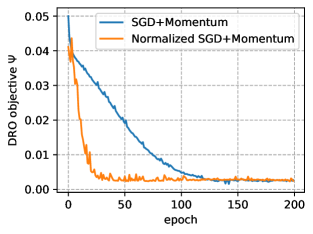
(a) Regression for $\chi^{2}$ penalized DRO

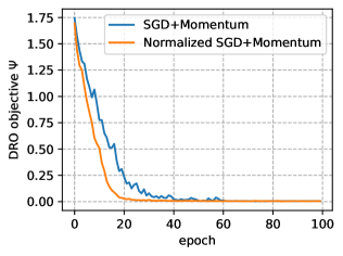
(b) Classification for $\chi^{2}$ penalized DRO

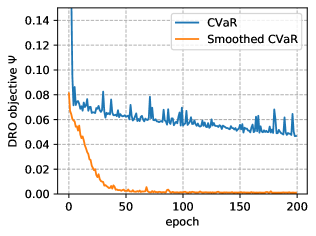
(c) Regression for smoothed CVaR

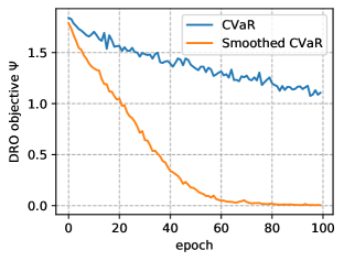
(d) Classification for smoothed CVaR

Figure 1: Training curve of $\chi^{2}$ penalized DRO and smoothed CVaR in regression and classification task.

4.2 Experimental results

Results are demonstrated in Figure 1. For each figure, we plot the value of the DRO objective $\Psi(x)$ through the training process. Here we calculate $\Psi(x)=\min_{\eta}\mathcal{L}(x,\eta)$ at each epoch based on a convex optimization on $\eta$ until convergence (rather than using ${\mathcal{L}}(x,\eta)$ with the current parameter $\eta$ directly).

Experimental result for $\chi^{2}$ penalized DRO. Figure 1(a) and Figure 1(b) plot the training curve of the DRO objective using different algorithms. It can be seen that in both regression and classification, vanilla SGD converges slowly, and using normalized momentum algorithm significantly improves the convergence speed. For example, in regression task SGD does not converge after 100 epochs while normalized momentum algorithm converges just after 25 epochs. These results highly consist with our theoretical findings, which shows that due to the non-smoothness of the DRO loss, vanilla SGD may not be able to optimize the loss well; In contrast, normalized momentum utilizes the relationship between local smoothness and gradient magnitude, and achieves better performance.

Experimental result for smoothed CVaR. Figure 1(c) and Figure 1(d) plot the training curves for different training losses: CVaR and smoothed CVaR. Note that the evaluation metrics ($y$-axis) in these figures are all chosen to be CVaR, even when the training objective is smoothed CVaR. In this way we can make a fair comparison of optimization speed based on these training curves. Firstly, it can be seen that the optimization of CVaR is very hard due to the non-smoothness, and the training curves have lots of spikes. In contrast, the optimization of smoothed CVaR is much easier for both tasks, and the final loss is significantly lower. Such experimental results show the benefit of our proposed smoothed CVaR for optimization.

Test performance. We also measure the test performance of trained models to see whether a better optimizer can also improve test accuracy. Due to space limitation, in the main text we provide results of $\chi^{2}$ penalized DRO problem for classification using unbalanced CIFAR-10 dataset, which is listed in Table 2. Other results can be found in Appendix E. It can be seen that the model trained using normalized SGD with momentum achieves higher test accuracy on all class, and especially, the worst-performing class. Since the experiments in this paper is mainly designed to compare algorithms rather than to achieve best performance, better performance is likely to be reached if adjusting the hyper-parameters (e.g. $\lambda$, the number of epochs, and the learning rate schedule).

Table 2: Test performance of the $\chi^{2}$ penalized DRO problem for unbalanced CIFAR-10 classification. Each column corresponds to the performance of a particular class. The bolded column indicates the worst-performing class.

Class	1	2	3	4	5	6	7	8	9	10
Number of training samples	4020	2715	4985	2965	1950	1425	4795	4030	4835	3300
Test acc (SGD+Momentum)	76.7	80.1	70.2	55.0	54.6	44.8	84.9	77.7	85.5	76.8
Test acc (Normalized SGD+Mom.)	78.8	81.2	71.7	57.3	56.2	49.8	87.2	83.5	90.4	78.4

5 Discussion

Conclusion. In this paper we provide non-asymptotic analysis of first-order algorithms for the DRO problem with unbounded and non-convex loss. Specifically, we write the original DRO problem as a non-smooth non-convex optimization problem, and we propose an efficient normalization-based algorithm to solve it. The general result of Theorem 3.5 might be of independent value and is not limited to DRO setting. We hope that this work can also bring inspiration to the study of other non-smooth non-convex optimization problems.

Limitations. Despite the theoretical grounds and promising experimental justifications, there are some interesting questions that remain unexplored. Firstly, it may be possible to obtain better complexities on problem-dependent parameters, e.g. $G$ and $\lambda$. Secondly, while this paper mainly considers smooth $\psi^{*}$, in some cases $\psi^{*}$ may be non-smooth (e.g. for KL-divergence) or even not continuous. In future we hope to discover approaches that can deal with more general classes of $\psi$-divergence. Finally, we are looking forward to seeing more applications of DRO in real-world problems.

Appendix A Equivalent formulation of the DRO objective

A.1 Generalized gradient

As can be seen, the problem 4 is the pointwise minima over $\eta$ for a family of smooth functions $\mathcal{L}(x,\eta)$. However, there exists a known result showing that the pointwise minima of a family of smooth functions may not be differentiable in general, so the gradient may not exist.

We first assume $\Psi(x)$ is non-smooth and non-convex. To measure the convergence of non-smooth non-convex optimization, we define the notion called the generalized gradient [Clarke, 1990, Chapter 2].

Definition A.1.

(Local Lipschitzness) A function $f:\mathcal{X}\to\mathbb{R}^{m}$ is locally Lipschitz continuous near point $x\in\operatorname{int}(\mathcal{X})$ if there exists $G,\epsilon>0$ such that for any $y,z\in\mathcal{B}_{\epsilon}(x)$, $|f(y)-f(z)|\leq G\left\|y-z\right\|$. Here $\mathcal{B}_{\epsilon}(x)$ denotes the set of points in the open ball of radius $\epsilon$ around $x$.

Definition A.2.

(Generalized gradient) Suppose that $f:\mathcal{X}\to\mathbb{R}$ is locally Lipschitz-continuous at $x$, where $\mathcal{X}\subset\mathbb{R}^{n}$. Its generalized directional derivative in direction $v$ is defined as

$$f^{\circ}(x;v)=\mathop{\operatorname{limsup}}_{\begin{subarray}{c}y\to x\\ t\to 0\end{subarray}}\frac{f(y+tv)-f(y)}{t}$$

and the generalized gradient at $x$ is the set

$$\partial f(x)=\left\{\zeta\in\mathbb{R}^{n}:f^{\circ}(x;v)\geq\left\langle\zeta,v\right\rangle\forall v\in\mathbb{R}^{n}\right\}.$$

Interested readers may refer to the book [Clarke, 1990] for an in-depth exploration of this concept. Importantly, $\partial f(x)$ is a non-empty closed convex set; $\partial f(x)$ degenerates to a single point $\{\nabla f(x)\}$ if $f$ is smooth, and $\partial f(x)$ is equivalent to the sub-gradient if $f$ is convex. If $x$ is a local minima (or maxima) for $f(x)$, then $0\in\partial f(x)$. The following proposition gives the relationship between generalized gradient and (conventional) gradient.

Proposition A.3.

([Clarke, 1990, Section 2.2]) If function $f$ is differentiable at $x$, then $f$ is local Lipschitz near $x$ and $\partial f(x)=\{\nabla f(x)\}$. Conversely, if $f$ is local Lipschitz near $x$ and $\partial f(x)$ reduces to a singleton point $\{g\}$, then $f$ is differentiable at $x$ and $\nabla f(x)=g$.

A.2 Proof of Lemma 2.6

We first present a basic lemma which provides a rule to calculate generalized gradients of the pointwise maxima of a function family.

Lemma A.4 ([Clarke, 1981]).

Suppose that $\mathcal{T}\subset\mathbb{R}^{m}$ is compact and $\mathcal{X}\subset\mathbb{R}^{n}$ is open. Let $f:\mathcal{X}\times\mathcal{T}\to\mathbb{R}$ be a $K$-Lipschitz continuous function in $x\in\mathcal{X}$ for some $K$ and is continuous in $t\in\mathcal{T}$. Define the point-wise minima function $F(x)=\min_{t\in\mathcal{T}}f(x,t)$, then we have

$$\partial F(x)\subset\operatorname{Conv}\bigcup_{t\in T(x)}\partial_{x}f(x,t)$$ (14)

where $T(x)=\left\{t\in T:F(x)=f(x,t)\right\}$, $\partial_{x}f(x,t)$ is the partial generalized gradient and $\operatorname{Conv}$ denotes a convex hull of a point set.

Recall that in our setting$\Psi(x)=\min_{\eta\in\mathbb{R}}\mathcal{L}(x,\eta)$. Since $\psi^{*}$ and $\ell$ are differentiable, $\mathcal{L}$ is differentiable in both $\eta$ and $x$. To make use of Lemma A.4, we have to constrain $\eta$ in a compact set $\mathcal{T}$. This is possible if we constrain $x$ in a compact set $\mathcal{B}_{r}(x_{0})$, an open ball of radius $r$ centered at $x_{0}$.

Lemma A.5.

Assume Assumption 2.4 holds. Fix a point $x_{0}\in\mathcal{X}$. Denote $\eta_{0}\in\operatorname{argmin}_{\eta}\mathcal{L}(x_{0},\eta)$ be an arbitrary minima. Then for any point $x\in\mathcal{B}_{r}(x_{0})$ near $x_{0},$ there exists $\eta_{x}\in\operatorname{argmin}_{\eta}\mathcal{L}(x,\eta)$, such that $|\eta_{0}-\eta_{x}|\leq Gr$.

Proof:

Using the condition that $\psi^{*}$ is convex and differentiable, we have $\eta_{x}\in\operatorname{argmin}_{\eta}\mathcal{L}(x,\eta)$ if and only if $\nabla_{\eta}\mathcal{L}(x,\eta)=0$. Namely,

$$\nabla_{\eta}\mathcal{L}(x,\eta)=1-\mathbb{E}_{\xi}\left[(\psi^{*})^{\prime}\left(\frac{\ell(x;\xi)-\eta_{x}}{\lambda}\right)\right]=0\quad\text{iff}\quad\eta_{x}\in\operatorname{argmin}_{\eta}\mathcal{L}(x,\eta).$$ (15)

For any point $x\in\mathcal{B}_{r}(x_{0})$, $|\ell(x;\xi)-\ell(x_{0};\xi)|\leq Gr$ holds for any $\xi$ due to the Lipschitz property of $\ell(\cdot;\xi)$. Considering that $(\psi^{*})^{\prime}$ is monotonically increasing (due to the convexity of $\psi^{*}$), we have

$$1-\mathbb{E}_{\xi}\left[(\psi^{*})^{\prime}\left(\frac{\ell(x;\xi)-(\eta_{0}+Gr)}{\lambda}\right)\right] \geq 0$$ (16)

$$1-\mathbb{E}_{\xi}\left[(\psi^{*})^{\prime}\left(\frac{\ell(x;\xi)-(\eta_{0}-Gr)}{\lambda}\right)\right] \leq 0$$ (17)

Since $\nabla_{\eta}\mathcal{L}(x,\eta)$ is continuous in $\eta$, there must exists an $\eta_{x}\in[\eta_{0}-Gr,\eta_{0}+Gr]$, such that

$$1-\mathbb{E}_{\xi}\left[(\psi^{*})^{\prime}\left(\frac{\ell(x;\xi)-\eta_{x}}{\lambda}\right)\right]=0$$ (18)

Therefore $\eta_{x}\in\operatorname{argmin}_{\eta}\mathcal{L}(x,\eta)$. $\square$

For any point $x_{0}$, we can use Lemma A.4 by substituting $\mathcal{X}=\mathcal{B}_{r}(x_{0})$ and $\mathcal{T}=[\eta_{0}-Gr,\eta_{0}+Gr]$. The procedure is as follows:

• $\Psi(x)=\min_{\eta\in\mathbb{R}}\mathcal{L}(x,\eta)=\min_{\eta\in[\eta_{0}-Gr,\eta_{0}+Gr]}\mathcal{L}(x,\eta)$ holds for all $x\in\mathcal{B}_{r}(x_{0})$;

• Applying Lemma A.4 we obtain

  $$\partial\Psi(x) \subset\operatorname{Conv}\{\nabla_{x}\mathcal{L}(x,\eta):\eta\in[\eta_{0}-Gr,\eta_{0}+Gr]\cap\operatorname{argmin}_{\eta}\mathcal{L}(x,\eta)\}$$

  $$\subset\operatorname{Conv}\{\nabla_{x}\mathcal{L}(x,\eta):\eta\in\operatorname{argmin}_{\eta}\mathcal{L}(x,\eta)\}$$

We finally prove below (Lemma A.6) that $\{\nabla_{x}\mathcal{L}(x,\eta):\eta\in\operatorname{argmin}_{\eta}\mathcal{L}(x,\eta)\}$ is a singleton set. Then Proposition A.3 indicates that $\Psi(x)$ is differentiable, and the generalized gradient reduces to gradient such that $\nabla\Psi(x)=\nabla_{x}\mathcal{L}(x,\eta)$ for any $\eta\in\operatorname{argmin}_{\eta}\mathcal{L}(x,\eta)$. Thus we complete the proof of Lemma 2.6.

Lemma A.6.

Assume Assumption 2.4 holds. For any $\eta_{1},\eta_{2}\in\operatorname{argmin}_{\eta}\mathcal{L}(x,\eta)$, we have $\nabla_{x}\mathcal{L}(x,\eta_{1})=\nabla_{x}\mathcal{L}(x,\eta_{2})$.

Proof:

Denote $X(x,\eta)$, $Y(x)$ be two random functions defined by

$$X(x,\eta)=(\psi^{*})^{\prime}\left(\frac{\ell(x;\xi)-\eta}{\lambda}\right)\quad Y(x)=\nabla_{x}\ell(x;\xi)$$

which depend on the random variable $\xi$. Rewrite the gradient of $\mathcal{L}(x,\eta)$ as follows:

$$\nabla_{x}\mathcal{L}(x,\eta) =\mathbb{E}[X(x,\eta)Y(x)]$$ (19)

$$\nabla_{\eta}\mathcal{L}(x,\eta) =1-\mathbb{E}[X(x,\eta)]$$ (20)

Note that $(\psi^{*})^{\prime}$ is monotonically increasing (due to the convexity of $\psi^{*}$), thus $X(x,\eta)$ is monotonically decreasing in $\eta$. It follows that

$$\nabla_{\eta}\mathcal{L}(x,\eta_{1})=\nabla_{\eta}\mathcal{L}(x,\eta_{2})\quad\text{iff}\quad\mathbb{E}[X(x,\eta_{1})]=\mathbb{E}[X(x,\eta_{2})]\quad\text{iff}\quad X(x,\eta_{1})=X(x,\eta_{2})\quad\text{a.s.}$$

Therefore $\mathbb{E}[X(x,\eta_{1})Y(x)]=\mathbb{E}[X(x,\eta_{2})Y(x)]$, namely $\nabla_{x}\mathcal{L}(x,\eta_{1})=\nabla_{x}\mathcal{L}(x,\eta_{2})$. $\square$

A.3 Proof of Theorem 2.7

Now, suppose that we have obtained a pair $(x,\eta)$ s.t. $\left\|\nabla_{x}\mathcal{L}(x,\eta)\right\|+G\left|\nabla_{\eta}\mathcal{L}(x,\eta)\right|\leq\epsilon$. Let $x$ be fixed and $\eta^{*}\in\mathop{\arg\min}_{\eta}\mathcal{L}(x,\eta)$. Then we have

$$\quad\left\|\nabla_{x}\mathcal{L}(x,\eta)-\nabla_{x}\mathcal{L}(x,\eta^{*})\right\|$$

$$=\left\|\mathbb{E}_{\xi}\left[\left(\left(\psi^{*}\right)^{\prime}\left(\frac{\ell(x;\xi)-\eta}{\lambda}\right)-\left(\psi^{*}\right)^{\prime}\left(\frac{\ell(x;\xi)-\eta^{*}}{\lambda}\right)\right)\nabla\ell(x;\xi)\right]\right\|$$

$$\leq G\cdot\mathbb{E}_{\xi}\left|\left(\psi^{*}\right)^{\prime}\left(\frac{\ell(x;\xi)-\eta}{\lambda}\right)-\left(\psi^{*}\right)^{\prime}\left(\frac{\ell(x;\xi)-\eta^{*}}{\lambda}\right)\right|$$

$$=G\cdot\left|\mathbb{E}_{\xi}\left[\left(\psi^{*}\right)^{\prime}\left(\frac{\ell(x;\xi)-\eta}{\lambda}\right)-\left(\psi^{*}\right)^{\prime}\left(\frac{\ell(x;\xi)-\eta^{*}}{\lambda}\right)\right]\right|$$

$$=G\left|\nabla_{\eta}\mathcal{L}(x,\eta)-\nabla_{\eta}\mathcal{L}(x,\eta^{*})\right|=G|\nabla_{\eta}\mathcal{L}(x,\eta)|$$

where we use the fact that $(\psi^{*})^{\prime}$ is monotone increasing (due to the comvexity of $\psi^{*}$. Hence, using Lemma 2.6 we obtain

$$\left\|\nabla\Psi(x)\right\|=\left\|\nabla_{x}\mathcal{L}(x,\eta^{*})\right\|\leq\left\|\nabla_{x}\mathcal{L}(x,\eta)\right\|+G\left|\nabla_{\eta}\mathcal{L}(x,\eta)\right|\leq\epsilon$$

Now suppose that $\|\nabla\widehat{\mathcal{L}}(x,\eta)\|\leq\epsilon/\sqrt{2}$. Then

$$\|\nabla\widehat{\mathcal{L}}(x,\eta)\|^{2}=\|\nabla_{x}{\mathcal{L}}(x,G\eta)\|^{2}+G^{2}|\nabla_{\eta}{\mathcal{L}}(x,G\eta)|^{2}\leq\epsilon^{2}/2$$

Using $(a+b)^{2}\leq 2(a^{2}+b^{2})$ we obtain

$$(\|\nabla_{x}{\mathcal{L}}(x,G\eta)\|+G|\nabla_{\eta}{\mathcal{L}}(x,G\eta)|)^{2}\leq\epsilon^{2}$$

which completes the proof.

Appendix B The Stochastic Projected Gradient Descent algorithm for DRO with bounded loss

In this section we use a simple projected gradient method to minimize the DRO objective (5) and analyze its convergence rate under the assumption that the loss is bounded. Since this section is not so related to the main result in our paper, we mainly provide the gradient complexity bound in terms of $\epsilon$ for finding an $\epsilon$-stationary point without delving into problem-dependent parameters.

Assumption B.1.

We have $0\leq\ell(x,\xi)\leq B$ for all $x\in\mathcal{X}$ and $\xi$.

It turns out that we can restrict the feasible region to $\mathcal{X}\times\left[{U},{V}\right]$ where $\left[{U},{V}\right]$ is a finite interval.

Proposition B.2.

Under the Assumptions 2.4 and B.1, the DRO problem is equivalent to

$$\operatorname{minimize}\widehat{\mathcal{L}}(x,\eta)\qquad\text{on}\quad(x,\eta)\in\mathcal{X}\times[U,V]$$ (21)

where $U=-\frac{\lambda C_{\psi}}{G}$ and $V=\frac{B-\lambda C_{\psi}}{G}$ are real numbers and $C_{\psi}$ is a constant depending only on $\psi$.

Proof:

Note that $(\psi^{*})^{\prime}$ is a function satisfying the following properties:

• $(\psi^{*})^{\prime}$ is monotonically increasing;

• $0\leq\lim\limits_{s\to-\infty}(\psi^{*})^{\prime}(s)\leq 1$. This is because $\lim\limits_{s\to-\infty}\frac{\psi^{*}(s)}{s}=\lim\limits_{s\to-\infty}\inf_{t\geq 0}t-\frac{\psi(t)}{s}=\min\{t:\psi(t)<+\infty\}\in[0,1]$ since $\psi(1)=0$;

• $\lim\limits_{s\to+\infty}(\psi^{*})^{\prime}(s)\geq 1$ (possibly be $+\infty$). This is because $\frac{\psi^{*}(s)}{s}=\sup_{t\geq 0}t-\frac{\psi(t)}{s}\geq 1$ for $s>0$ since $\psi(1)=0$.

Therefore there exists a constant $C_{\psi}$ depending only on $\psi$ such that $(\psi^{*})^{\prime}(C_{\psi})=1$.

For any $x\in\mathcal{X}$, the optimal $\eta^{*}$ satisfies the following equation:

$$\mathbb{E}\left[(\psi^{*})^{\prime}\left(\frac{\ell(x;\xi)-G\eta^{*}}{\lambda}\right)\right]=1.$$ (22)

We now show there exists an optimal $\eta^{*}$ such that $G\eta^{*}\in[-\lambda C_{\psi},B-\lambda C_{\psi}]$. In fact, we have

• For any $G\eta<-\lambda C_{\psi}$, $\mathbb{E}\left[(\psi^{*})^{\prime}\left(\frac{\ell(x;\xi)-G\eta}{\lambda}\right)\right]\geq\mathbb{E}\left[(\psi^{*})^{\prime}\left(\frac{-\eta}{\lambda}\right)\right]\geq(\psi^{*})^{\prime}(C_{\psi})=1$;

• For any $G\eta>B-\lambda C_{\psi}$, $\mathbb{E}\left[(\psi^{*})^{\prime}\left(\frac{\ell(x;\xi)-G\eta}{\lambda}\right)\right]\leq\mathbb{E}\left[(\psi^{*})^{\prime}\left(\frac{B-\eta}{\lambda}\right)\right]\leq(\psi^{*})^{\prime}(C_{\psi})=1$.

We conclude the proof by noting that $\mathbb{E}\left[(\psi^{*})^{\prime}\left(\frac{\ell(x;\xi)-G\eta}{\lambda}\right)\right]$ is monotonically decreasing in $\eta$. $\square$

Since $\eta$ is constrained in a finite interval $[U,V]$, we propose to solve 21 using the randomized stochastic projected gradient (RSPG) algorithm [Ghadimi et al., 2016]. It is summarized in Algorithm 2. Note that the algorithm can deal with situations when the feasible set $\mathcal{X}\in\mathbb{R}^{d}$ is also constrained.

Input : Feasible region $\mathcal{K}$, objective function $F(w)$, distribution $P$, initial point $w_{0}\in\mathcal{K}$, step size $\gamma$, mini-batch sizes $S$, and total number of iterations $T$

1 for $t\leftarrow 1$ to $T$ do

2       $\{\xi_{t-1}^{(i)}\}_{i=1}^{S}\leftarrow\text{i.i.d. samples drawn from }P$;

3       $\hat{\nabla}F(w_{t-1})\leftarrow\frac{1}{S}\sum_{i=1}^{S}\nabla F(w_{t-1},\xi_{t-1}^{(i)})$;

4       $w_{t}\leftarrow\Pi_{\mathcal{K}}(w_{t-1}-\gamma\hat{\nabla}F(w_{t-1}))\text{ where }\Pi_{\mathcal{K}}\text{is the projection onto }\mathcal{K}$;

5      

Output : randomly return one $w_{t}$ in $\{w_{t}\}_{t=1}^{T}$

Algorithm 2 Randomized stochastic projected gradient (RSPG)

Proposition B.3.

Suppose Assumption 2.4 holds. Under Proposition B.2, $\mathcal{L}$ is $K$ smooth on $\mathcal{X}\times[U,V]$, where $K$ only depends on $\psi,\lambda,M,B,G$ and $L$.

Proof:

First note that $\left(\psi^{*}\right){{}^{\prime}}$ is $M$-Lipschitz continuous, and the range of $\frac{\ell(x,\xi)-G\eta}{\lambda}$ lies in the interval $\left[C_{\psi}-\lambda^{-1}B,C_{\psi}+\lambda^{-1}B\right]$, thus $\left(\psi^{*}\right){{}^{\prime}}\left(\frac{\ell(x;\xi)-G\eta}{\lambda}\right)$ is bounded by a constant $\left|\left(\psi^{*}\right){{}^{\prime}}\left(\frac{\ell(x;\xi)-G\eta}{\lambda}\right)\right|\leq\left(\psi^{*}\right){{}^{\prime}}(C_{\psi}+\lambda^{-1}B)$.

$$\quad\|\nabla_{x}\mathcal{L}(x_{1},\eta_{1})-\nabla_{x}\mathcal{L}(x_{2},\eta_{2})\|$$

$$=\left\|\mathbb{E}_{\xi\sim P}\left[\left(\psi^{*}\right){{}^{\prime}}\left(\frac{\ell(x_{1};\xi)-G\eta_{1}}{\lambda}\right)\cdot\nabla\ell(x_{1},\xi)-\left(\psi^{*}\right){{}^{\prime}}\left(\frac{\ell(x_{2};\xi)-G\eta_{2}}{\lambda}\right)\cdot\nabla\ell(x_{2},\xi)\right]\right\|$$

$$\leq\mathbb{E}_{\xi\sim P}\left[\left(\psi^{*}\right){{}^{\prime}}(C_{\psi}+\lambda^{-1}B)\left\|\nabla\ell(x_{1},\xi)-\nabla\ell(x_{2},\xi)\right\|\right]$$

$$\quad+\mathbb{E}_{\xi\sim P}\left[G\left|\left(\psi^{*}\right){{}^{\prime}}\left(\frac{\ell(x_{1};\xi)-G\eta_{1}}{\lambda}\right)-\left(\psi^{*}\right){{}^{\prime}}\left(\frac{\ell(x_{2};\xi)-G\eta_{2}}{\lambda}\right)\right|\right]$$

$$\leq\left(\psi^{*}\right){{}^{\prime}}(C_{\psi}+\lambda^{-1}B)L\|x_{1}-x_{2}\|+\lambda^{-1}GM\left(G\|x_{1}-x_{2}\|+G\left|\eta_{1}-\eta_{2}\right|\right)$$

Similarly we can show that

$$\|\nabla_{\eta}\mathcal{L}(x_{1},\eta_{1})-\nabla_{\eta}\mathcal{L}(x_{2},\eta_{2})\|\leq G\lambda^{-1}M\left(G\|x_{1}-x_{2}\|+G\left|\eta_{1}-\eta_{2}\right|\right)$$ (23)

Therefore $\mathcal{L}$ is smooth. $\square$

Proposition B.4.

Suppose Assumption 2.4 holds. Under Proposition B.2, the stochastic gradients are unbiased estimates of the true gradients $\nabla_{x}\mathcal{L}$ and $\nabla_{\eta}\mathcal{L}$ and are uniformly bounded over $\mathcal{X}\times{[U,V]}$, by a constant $\Lambda$ which only depends on $\psi,\lambda,M,B,G$ and $L$.

Proof:

As we have shown in the proof of Proposition B.3, the term $\left(\psi^{*}\right){{}^{\prime}}\left(\frac{\ell(x;\xi)-G\eta}{\lambda}\right)$ is bounded by $\left(\psi^{*}\right){{}^{\prime}}(C_{\psi}+\lambda^{-1}B)$. Then it’s easy to see that $\nabla_{x}\mathcal{L}(x,\eta;\xi)$ and $\nabla_{\eta}\mathcal{L}(x,\eta;\xi)$ are bounded and the squared norm of true gradient is bounded by $\Lambda^{2}=2\left[(\psi^{*}){{}^{\prime}}(C_{\psi}+\lambda^{-1}B)\right]^{2}G^{2}+G^{2}$. $\square$

Following [Ghadimi et al., 2016, Reddi et al., 2016], in constrained optimization we typically consider a generalized gradient defined as

$$\mathcal{P}_{\mathcal{X}}(x,\nabla f(x),\gamma)=\frac{1}{\gamma}(x-x^{+}),\quad\text{where }x^{+}=\arg\min_{u\in\mathcal{X}}\left\{\left\langle\nabla f(x),u\right\rangle+\frac{1}{2\gamma}\|u-x\|^{2}\right\}$$

Note that $x^{+}$ is exactly the projection of $x-\gamma\nabla f(x)$ onto the set $\mathcal{X}$. For unconstrained optimization when $\mathcal{X}=\mathbb{R}^{d}$, this definition coincides with the gradient in the traditional sense. We say that $x$ is an $\epsilon$-stationary point if $\left\|\mathcal{P}_{\mathcal{X}}(x,\nabla f(x),\gamma)\right\|\leq\epsilon$. The above propositions combined with  [Ghadimi et al., 2016, Corollary 3] imply the following convergence result.

Theorem B.5.

Suppose Assumptions 2.4 and B.1 hold. With $\mathcal{K}=\mathcal{X}\times[U,V]$, $w_{0}=(x_{0},\eta_{0})$ and properly chosen $\gamma$ and $S$, Algorithm 2 finds an $\epsilon$-stationary point with complexity $\mathcal{O}(\Lambda^{2}K\Delta\epsilon^{-4})$,where $\Delta=\mathcal{L}(x_{0},\eta_{0})-\inf_{(x,\eta)\in\mathcal{X}\times\mathbb{R}}\mathcal{L}(x,\eta)$ and $K,\Lambda$ are constants that appeared in Propositions B.3 and B.4. Moreover, with the choice $T=4K\Delta\epsilon^{-2}$, $\gamma=1/2L$ and $S=24\Lambda^{2}\epsilon^{-2}$, Algorithm 2 finds an $\epsilon$-stationary point with probability $\geq 0.5$.

Proof:

[Ghadimi et al., 2016, Corollary 3], combined with Proposition B.4 implies that if $\gamma=1/2L$,

$$\mathbb{E}\left[\left\|\mathcal{P}_{\mathcal{X}\times{[U,V]}}((x_{k},\eta_{k}),\nabla\mathcal{L}(x_{k},\eta_{k}),\gamma)\right\|^{2}\right]\leq\frac{K\Delta}{T}+\frac{6\Lambda^{2}}{S}.$$ (24)

For any $\epsilon>0$, we choose $T=2K\Delta\epsilon^{-2}$ and $S=12\Lambda^{2}\epsilon^{-2}$, then 24 implies that

$$\mathbb{E}\left[\left\|\mathcal{P}_{\mathcal{X}\times{[U,V]}}((x_{k},\eta_{k}),\nabla\mathcal{L}(x_{k},\eta_{k}),\gamma)\right\|^{2}\right]\leq\epsilon$$ (25)

Thus the sample complexity of Algorithm 1 for finding $\epsilon$-stationary point is upper bounded by $24K\Lambda^{2}\Delta\epsilon^{-4}$. In this case, with pobability $\geq 0.5$ the gradient norm is upper bounded by $2\epsilon$, the conclusion follows. $\square$

While the above theorem provides non-asymptotic convergence rate to a stationary point, note that the definition of generalized gradient involves the interval $[{U,V}]$ which was constructed artificially for Algorithm 2, thus $\mathbb{E}\left[\|\mathcal{P}_{\mathcal{X}\times{[U,V]}}((x_{k},\eta_{k}),\nabla\widehat{\mathcal{L}}(x_{k},\eta_{k}),\gamma)\|^{2}\right]\leq\epsilon$ does not necessarily lead to an $\epsilon$-stationary point of $\nabla\widehat{\mathcal{L}}$. We then show below that the generalized gradient is indeed equal to the true gradient in the unconstrained case $\mathcal{X}=\mathbb{R}^{n}$, therefore Theorem B.5 corresponds to the gradient complexity for finding an $\epsilon$-stationary point of $\Psi(x)$.

Theorem B.6.

Consider the unconstrained case $\mathcal{X}=\mathbb{R}^{n}$. Choose

$$\tilde{U}=-\frac{\lambda C_{\psi}}{G}-\frac{\epsilon}{L},\quad\tilde{V}=\frac{B-\lambda C_{\psi}}{G}+\frac{\epsilon}{L}$$

as the interval constraint for $\eta$. Using parameters specified in Theorem B.5, Algorithm 2 arrives at $(x,\eta)$ with $\left\|\nabla\Psi(x)\right\|\leq\epsilon$ with probability $\geq 0.5$.

Proof:

It suffices to show that: whenever $\|\mathcal{P}_{\mathbb{R}^{n}{\times[\tilde{U},\tilde{V}]}}((x,\eta),\nabla\widehat{\mathcal{L}}(x,\eta),\gamma)\|\leq\epsilon$, we must have $\|\nabla\widehat{\mathcal{L}}(x,\eta)\|\leq\epsilon$.

Recall that

$$\mathcal{P}_{\mathbb{R}^{n}{\times[\tilde{U},\tilde{V}]}}((x,\eta),\nabla\widehat{\mathcal{L}}(x,\eta),\gamma)=\frac{1}{\gamma}(x-x^{+},\eta-\eta^{+})$$ (26)

where

$$x^{+} =\arg\min_{u\in\mathbb{R}^{n}}\left\{\left\langle\nabla_{x}\widehat{\mathcal{L}}(x,\eta),u\right\rangle+\frac{1}{2\gamma}\|u-x\|^{2}\right\}$$ (27)

$$\eta^{+} =\arg\min_{\rho\in{[\tilde{U},\tilde{V}]}}\left\{\rho\nabla_{\eta}\widehat{\mathcal{L}}(x,\eta)+\frac{1}{2\gamma}(\rho-\eta)^{2}\right\}$$

Define $\eta_{0}:=\eta-\gamma\nabla_{\eta}\widehat{\mathcal{L}}(x,\eta)$. Since $\|\mathcal{P}_{\mathbb{R}^{n}{\times[\tilde{U},\tilde{V}]}}((x,\eta),\nabla\widehat{\mathcal{L}}(x,\eta),\gamma)\|\leq\epsilon$, we have $\left|\eta-\eta^{+}\right|\leq\gamma\epsilon$. We consider two possible cases below:

• Case 1. $\eta^{+}\in{(\tilde{U},\tilde{V})}$. In this case it is easy to see that $\eta^{+}=\eta_{0}$ and thus

  $$\|\nabla\widehat{\mathcal{L}}(x,\eta)\|=\|\mathcal{P}_{\mathbb{R}^{n}{\times[\tilde{U},\tilde{V}]}}((x,\eta),\nabla\widehat{\mathcal{L}}(x,\eta),\gamma)\|\leq\epsilon$$

• Case 2. $\eta^{+}\in\{{\tilde{U},\tilde{V}}\}$. Assume that $\eta^{+}=\tilde{U}$ (the case $\eta^{+}=\tilde{V}$ is similar). Then $\eta\in[\tilde{U},\tilde{U}+\gamma\epsilon]$. Note that $\tilde{U}+\gamma\epsilon=-\frac{\lambda C_{\psi}}{G}+\frac{\epsilon}{2L}<U$. In this case, $\left(\psi^{*}\right)^{\prime}\left(\frac{\ell(x,\xi)-\eta}{\lambda}\right)\geq 1$. Therefore

  $$\eta_{0}=\eta-\gamma\nabla_{\eta}\widehat{\mathcal{L}}(x,\eta)=\eta-G\gamma\left(1-\mathbb{E}\left[\left(\psi^{*}\right)^{\prime}\left(\frac{\ell(x,\xi)-G\eta}{\lambda}\right)\right]\right)\geq\eta.$$

  However, $\eta^{+}\leq\eta$, therefore it can only be that $\eta^{+}=\eta=\eta_{0}$. Therefore we still have

  $$\|\nabla\widehat{\mathcal{L}}(x,\eta)\|=\|\mathcal{P}_{\mathbb{R}^{n}{\times[\tilde{U},\tilde{V}]}}((x,\eta),\nabla\widehat{\mathcal{L}}(x,\eta),\gamma)\|\leq\epsilon$$

$\square$

In the above theorem, the constraint of $\eta$ is $[\tilde{U},\tilde{V}]$ which strictly contains $\eta\in[U,V]$ (in Proposition B.2). Nevertheless, the difference of the endpoints between $U$($V$) and $\tilde{U}$($\tilde{V}$) is only $\mathcal{O}(\epsilon)$. Therefore it does not change the final gradient complexity of $\mathcal{O}(\epsilon^{4})$ in Theorem B.5.

Appendix C Proofs in Section 3.2

In this section we present the proof of main results in Section 3.2. For convenience we restate the results before proving them.

C.1 Proofs of Lemmas 3.3 and 3.4

Lemma C.1.

Under Assumptions 2.4 and 3.2, the gradient estimators of (5) satisfies the following property:

$$\mathbb{E}_{\xi}\|\nabla\widehat{\mathcal{L}}(x,\eta,\xi)-\nabla\widehat{\mathcal{L}}(x,\eta)\|^{2}\leq 11G^{2}M^{2}\lambda^{-2}\sigma^{2}+8(G^{2}+\|\nabla\widehat{\mathcal{L}}(x,\eta)\|^{2})$$ (28)

Proof:

For a random vector $X$, define the sum of its element-wise variance as

$$\mathbb{V}\left(X\right):=\mathbb{E}\left\|X-\mathbb{E}[X]\right\|_{2}^{2},$$ (29)

Then it is easy to check that, for i.i.d. random vectors $X_{1},X_{2}$ we have

$$\mathbb{E}\left\|X_{1}-X_{2}\right\|^{2}=2\mathbb{V}[X_{1}].$$ (30)

We first bound the variance of the stochastic gradient $\nabla_{x}\widehat{\mathcal{L}}(x,\eta;\xi)$. Indeed we have

$$\quad\mathbb{V}\left[\nabla_{x}\widehat{\mathcal{L}}(x,\eta;\xi)\right]$$ (31)

$$=\frac{1}{2}\mathbb{E}_{\xi_{1},\xi_{2}}\left\|\left(\psi^{*}\right){{}^{\prime}}\left(\frac{\ell(x;\xi_{1})-G\eta}{\lambda}\right)\cdot\nabla\ell(x,\xi_{1})-\left(\psi^{*}\right){{}^{\prime}}\left(\frac{\ell(x;\xi_{2})-G\eta}{\lambda}\right)\cdot\nabla\ell(x,\xi_{2})\right\|^{2}$$ (32)

$$\leq\mathbb{E}_{\xi_{1},\xi_{2}}\left[\left(\left(\psi^{*}\right){{}^{\prime}}\left(\frac{\ell(x;\xi_{1})-G\eta}{\lambda}\right)\right)^{2}\left\|\nabla\ell(x,\xi_{1})-\nabla\ell(x,\xi_{2})\right\|^{2}\right]$$

$$\quad+\mathbb{E}_{\xi_{1},\xi_{2}}\left[\left\|\nabla\ell(x,\xi_{2})\right\|^{2}\left(\left(\psi^{*}\right){{}^{\prime}}\left(\frac{\ell(x;\xi_{1})-G\eta}{\lambda}\right)-\left(\psi^{*}\right){{}^{\prime}}\left(\frac{\ell(x;\xi_{2})-G\eta}{\lambda}\right)\right)^{2}\right]$$ (33)

$$\leq 4G^{2}\mathbb{E}_{\xi_{1}}\left[\left(\left(\psi^{*}\right){{}^{\prime}}\left(\frac{\ell(x;\xi_{1})-G\eta}{\lambda}\right)\right)^{2}\right]+G^{2}M^{2}\lambda^{-2}\mathbb{E}_{\xi_{1},\xi_{2}}\left[\left(\ell(x,\xi_{1})-\ell(x,\xi_{2})\right)^{2}\right]$$ (34)

$$\leq 4G^{2}\mathbb{E}_{\xi_{1}}\left[\left(\left(\psi^{*}\right){{}^{\prime}}\left(\frac{\ell(x;\xi_{1})-G\eta}{\lambda}\right)\right)^{2}\right]+2G^{2}M^{2}\lambda^{-2}\sigma^{2}$$ (35)

Here in 33 we use that fact that $(a+b)^{2}\leq 2(a^{2}+b^{2})$ for any $a,b$; in 34 we use Assumption 2.4. Now we deal with the first term. Using $2(a-1)^{2}+2\geq a^{2}$ for any $a$, we have

$$\mathbb{E}_{\xi}\left[\left(\left(\psi^{*}\right){{}^{\prime}}\left(\frac{\ell(x;\xi)-G\eta}{\lambda}\right)\right)^{2}\right] \leq 2+2\mathbb{E}_{\xi}\left[\left(1-\left(\psi^{*}\right){{}^{\prime}}\left(\frac{\ell(x;\xi)-G\eta}{\lambda}\right)\right)^{2}\right]$$ (36)

$$\leq 2\left(1+G^{-2}\|\nabla_{\eta}\widehat{\mathcal{L}}(x,\eta)\|^{2}+G^{-2}\mathbb{V}[\nabla_{\eta}\widehat{\mathcal{L}}(x,\eta;\xi)]\right)$$

Next, $\mathbb{V}[\nabla_{\eta}\widehat{\mathcal{L}}(x,\eta;\xi)]$ can be easily bounded as follows:

$$\mathbb{V}[\nabla_{\eta}\widehat{\mathcal{L}}(x,\eta;\xi)] =\frac{1}{2}G^{2}\mathbb{E}_{\xi_{1},\xi_{2}}\left[\left(\left(\psi^{*}\right){{}^{\prime}}\left(\frac{\ell(x;\xi_{1})-G\eta}{\lambda}\right)-\left(\psi^{*}\right){{}^{\prime}}\left(\frac{\ell(x;\xi_{2})-G\eta}{\lambda}\right)\right)^{2}\right]$$ (37)

$$\leq G^{2}M^{2}\lambda^{-2}\sigma^{2}$$

Combining with 35, 36 and 37, we obtain

$$\mathbb{V}[\nabla_{x}\widehat{\mathcal{L}}(x,\eta;\xi)] \leq 2G^{2}M^{2}\lambda^{-2}\sigma^{2}+8(G^{2}+\|\nabla_{\eta}\widehat{\mathcal{L}}(x,\eta)\|^{2}+G^{2}M^{2}\lambda^{-2}\sigma^{2})$$

$$=10G^{2}M^{2}\lambda^{-2}\sigma^{2}+8(G^{2}+\|\nabla_{\eta}\widehat{\mathcal{L}}(x,\eta)\|^{2})$$

$$\leq 10G^{2}M^{2}\lambda^{-2}\sigma^{2}+8(G^{2}+\|\nabla\widehat{\mathcal{L}}(x,\eta)\|^{2})$$

Finally,

$$\mathbb{V}[\nabla\widehat{\mathcal{L}}(x,\eta;\xi)] =\mathbb{V}[\nabla_{x}\widehat{\mathcal{L}}(x,\eta;\xi)]+\mathbb{V}[\nabla_{\eta}\widehat{\mathcal{L}}(x,\eta;\xi)]$$

$$\leq 11G^{2}M^{2}\lambda^{-2}\sigma^{2}+8(G^{2}+\|\nabla\widehat{\mathcal{L}}(x,\eta)\|^{2})$$

$\square$

Lemma C.2.

Under Assumption 2.4, for any pair of parameters $(x,\eta)$ and $(x^{\prime},\eta^{\prime})$, we have the following property for the gradient of $\widehat{\mathcal{L}}$:

$$\|\nabla\widehat{\mathcal{L}}(x,\eta)-\nabla\widehat{\mathcal{L}}(x^{\prime},\eta^{\prime})\|\leq\left(K+\tfrac{L}{G}\|\nabla\widehat{\mathcal{L}}(x,\eta)\|\right)\|(x-x^{\prime},\eta-\eta^{\prime})\|$$ (38)

where $K=L+2G^{2}\lambda^{-1}M$.

Proof:

First write $\nabla\widehat{\mathcal{L}}(x,\eta)$ as

$$\nabla\widehat{\mathcal{L}}(x,\eta)=\mathbb{E}_{\xi}\left[\left((\psi^{*})^{\prime}\left(\frac{\ell(x;\xi)-G\eta}{\lambda}\right)\nabla\ell(x,\xi),G-G(\psi^{*})^{\prime}\left(\frac{\ell(x;\xi)-G\eta}{\lambda}\right)\right)^{T}\right]$$ (39)

We then split $\nabla\mathcal{L}(x,\eta)-\nabla\mathcal{L}(x^{\prime},\eta^{\prime})$ into two terms $A+B$, where

$$A =\mathbb{E}_{\xi}\left[\left((\psi^{*})^{\prime}\left(\frac{\ell(x;\xi)-G\eta}{\lambda}\right)(\nabla\ell(x;\xi)-\nabla\ell(x^{\prime};\xi)),0\right)^{T}\right]$$ (40)

$$B =\mathbb{E}_{\xi}\left[\left((\psi^{*})^{\prime}\left(\frac{\ell(x;\xi)-G\eta}{\lambda}\right)-(\psi^{*})^{\prime}\left(\frac{\ell(x^{\prime};\xi)-G\eta^{\prime}}{\lambda}\right)\right)\left(\nabla\ell(x^{\prime};\xi),-G\right)^{T}\right].$$

$A$ can be bounded as follows:

$$\|A\|\leq L\cdot\mathbb{E}_{\xi}\left[(\psi^{*})^{\prime}\left(\frac{\ell(x;\xi)-G\eta}{\lambda}\right)\|x-x^{\prime}\|\right]$$ (41)

where we use $(\psi^{*})^{\prime}(s)\geq 0$ for all $s$. $B$ can be bounded as follows:

$$\|B\| \leq\sqrt{2}G\cdot\mathbb{E}_{\xi}\left[\left|(\psi^{*})^{\prime}\left(\frac{\ell(x;\xi)-G\eta}{\lambda}\right)-(\psi^{*})^{\prime}\left(\frac{\ell(x^{\prime};\xi)-G\eta^{\prime}}{\lambda}\right)\right|\right]$$ (42)

$$\leq\sqrt{2}G\lambda^{-1}M\mathbb{E}_{\xi}\left[\left|(\ell(x;\xi)-\ell(x^{\prime};\xi))-G(\eta-\eta^{\prime})\right|\right]$$

$$\leq 2G^{2}\lambda^{-1}M\|(x,\eta)^{T}-(x^{\prime},\eta^{\prime})^{T}\|$$

where the last step is because the function $(x,\eta)\to\ell(x,\xi)-G\eta$ is $\sqrt{2}G$ Lipschitz. Finally we bound $\mathbb{E}_{\xi}\left[(\psi^{*})^{\prime}\left(\frac{\ell(x;\xi)-G\eta}{\lambda}\right)\right]$ using the true gradient of $\widehat{\mathcal{L}}$:

$$\mathbb{E}_{\xi}\left[(\psi^{*})^{\prime}\left(\frac{\ell(x;\xi)-G\eta}{\lambda}\right)\right]=1-G^{-1}\nabla_{\eta}\widehat{\mathcal{L}}(x,\eta)\leq 1+G^{-1}|\nabla_{\eta}\widehat{\mathcal{L}}(x,\eta)|$$

Combining the above inequalities, we obtain

$$\quad\|\nabla\widehat{\mathcal{L}}(x,\eta)-\nabla\widehat{\mathcal{L}}(x^{\prime},\eta^{\prime})\|\leq\|A\|+\|B\|$$

$$\leq(L+LG^{-1})|\nabla_{\eta}\widehat{\mathcal{L}}(x,\eta)|\|x-x^{\prime}\|+2G^{2}\lambda^{-1}M\|(x-x^{\prime},\eta-\eta^{\prime})^{T}\|$$

$$\leq\left(L+2G^{2}\lambda^{-1}M+\tfrac{L}{G}\|\nabla\widehat{\mathcal{L}}(x,\eta)\|\right)\|(x-x^{\prime},\eta-\eta^{\prime})\|$$

which concludes the proof. $\square$

C.2 Proof of Theorem 3.5

C.2.1 Properties of generalized smoothness

We formalize the generalized smoothness property into a definition.

Definition C.3.

A continuously differentiable function $F:\mathbb{R}^{d}\to\mathbb{R}$ is said to be $(K_{0},K_{1})$-smooth if $\left\|\nabla F(x)-\nabla F(y)\right\|\leq(K_{0}+K_{1}\left\|\nabla F(x)\right\|)\|x-y\|$ for all $x,y\in\mathbb{R}^{d}$.

We now present a descent inequality for $(K_{0},K_{1})$-smooth functions which will be used in subsequent analysis.

Lemma C.4.

(Descent Inequality) Let $F$ be $(K_{0},K_{1})$-smooth, then for any point $x$ and direction $z$ the following holds:

$$F\left(x-z\right)\leq F\left(x\right)-\left\langle\nabla F\left(x\right),z\right\rangle+\frac{1}{2}(K_{0}+K_{1}\left\|\nabla F(x)\right\|)\left\|z\right\|^{2}.$$ (43)

Proof:

By definition we have

$$F(x-z)-F(x)-\left\langle z,\nabla F(x)\right\rangle =\int_{0}^{1}\left\langle\nabla F\left(x-\theta z\right)-\nabla F(x),z\right\rangle\text{d}\theta$$ (44)

$$\leq\int_{0}^{1}\|\nabla F\left(x-\theta z\right)-\nabla F(x)\|\|z\|\text{d}\theta$$

$$\leq\int_{0}^{1}\left(K_{0}\theta\|z\|^{2}+K_{1}\theta\|z\|^{2}\|\nabla F(x)\|\right)\text{d}\theta$$

$$=\dfrac{K_{0}+K_{1}\|\nabla F(x)\|}{2}\|z\|^{2}$$

so the conclusion follows. $\square$

C.2.2 Properties of the normalized update

We begin with a simple algebraic lemma.

Lemma C.5.

Let $\mu\geq 0$ be a real constant. For any vectors $u$ and $v$,

$$-\frac{\left\langle u,v\right\rangle}{\|v\|}\leq-\mu\|u\|-(1-\mu)\|v\|+(1+\mu)\|v-u\|$$ (45)

Proof:

$$-\frac{\left\langle u,v\right\rangle}{\|v\|} =-\|v\|+\frac{\left\langle v-u,v\right\rangle}{\|v\|}$$

$$\leq-\|v\|+\|v-u\|$$

$$\leq-\|v\|+\|v-u\|+\mu(\|v-u\|+\|v\|-\|u\|)$$

$$=-\mu\|u\|-(1-\mu)\|v\|+(1+\mu)\|v-u\|$$

$\square$

Now we can characterize the behavior of normalization-based algorithms in terms of function value descent.

Lemma C.6.

Consider the algorithm that starts at $w_{0}$ and makes updates $w_{t+1}=w_{t}-\gamma\frac{m_{t+1}}{\left\|m_{t+1}\right\|}$ where $\{m_{t}\}$ is an arbitrary sequence of points. Define $\delta_{t}:=m_{t+1}-\nabla F(w_{t})$ be the estimation error. Then

$$F(w_{t+1})-F(w_{t})\leq-\left(\gamma-\frac{1}{2}K_{1}\gamma^{2}\right)\|\nabla F(w_{t})\|+\frac{1}{2}K_{0}\gamma^{2}+2\gamma\|\delta_{t}\|$$

And thus by a telescope sum we have

$$\left(1-\frac{1}{2}K_{1}\gamma\right)\sum_{t=0}^{T-1}\|\nabla F(w_{t})\|\leq\dfrac{F(w_{0})-F(w_{T})}{\gamma}+\frac{1}{2}K_{0}T\gamma+2\sum_{t=0}^{T-1}\|\delta_{t}\|$$

Proof:

Since $\|w_{t+1}-w_{t}\|=\gamma$, by Lemma C.4 we have

$$F(w_{t+1})-F(w_{t}) \leq-\frac{\gamma}{\|m_{t+1}\|}\left\langle\nabla F(w_{t}),m_{t+1}\right\rangle+\frac{1}{2}\gamma^{2}\left(K_{0}+K_{1}\|\nabla F(w_{t})\|\right)$$

$$\leq\gamma\left(-\|\nabla F(w_{t})\|+2\|\delta_{t}\|\right)+\dfrac{1}{2}\gamma^{2}\left(K_{0}+K_{1}\|\nabla F(w_{t})\|\right)$$

$$=-\left(\gamma-\frac{1}{2}K_{1}\gamma^{2}\right)\|\nabla F(w_{t})\|+\frac{1}{2}K_{0}\gamma^{2}+2\gamma\|\delta_{t}\|$$

where in the second inequality we use Lemma C.5. $\square$

C.2.3 A general convergence result

Instead of directly focusing on the specific problem of DRO, we first provide convergence guarantee for Algorithm 2 under general smoothness and noise assumptions.

Theorem C.7.

Suppose that $F$ is $(K_{0},K_{1})$-smooth and the stochastic gradient estimator $\nabla F(w,\xi)$ is unbiased and satisfies

$$\mathbb{E}\left\|\nabla F(w,\xi)-\nabla F(w)\right\|^{2}\leq\Gamma^{2}\left\|\nabla F(w)\right\|^{2}+\Lambda^{2}$$

Let $\{w_{t}\}$ be the sequence produced by Algorithm 1, then with a mini-batch size ${S}=64\Gamma^{2}$ and a suitable choice of parameters $\gamma$ and $\beta$, for any small $\epsilon\leq\mathcal{\min}\left(\frac{K_{0}}{K_{1}},\frac{\Lambda}{2\Gamma}\right)$, we need at most $512\Delta K_{0}\Lambda^{2}\epsilon^{-4}$ gradient complexity to guarantee that we find an $2\epsilon$-first-order stationary point in expectation, i.e. $\frac{1}{T}\sum_{t=0}^{T-1}\mathbb{E}\|\nabla F(w_{t})\|\leq 2\epsilon$ where $\Delta=F(w_{0})-\inf_{w\in\mathbb{R}^{d}}F(w)$.

Proof:

Define the estimation errors $\delta_{t}:=m_{t+1}-\nabla F(w_{t})$. Denote $H(a,b):=\nabla F(a)-\nabla F(b)$. We can upper bound $H(a,b)$ using the definition of $(K_{0},K_{1})$-smoothness:

$$\|H(a,b)\|\leq\|a-b\|\left(K_{0}+K_{1}\|\nabla F(a)\|\right)$$ (46)

Using the definition of momentum $m_{t}$ and $H(a,b)$, we can get a recursive formula on $\delta_{t}$:

$$\delta_{t+1} =\beta m_{t+1}+(1-\beta)\hat{\nabla}F(w_{t+1})-\nabla F(w_{t+1})$$ (47)

$$=\beta\delta_{t}+\beta H\left(w_{t},w_{t+1}\right)+(1-\beta)(\hat{\nabla}F(w_{t+1})-\nabla F(w_{t+1}))$$

Denote $\hat{\delta}_{t}=\hat{\nabla}F(w_{t})-\nabla F(w_{t})$ be the stochastic noise, then the variance of $\hat{\delta}_{t}$ can be bounded by $\mathbb{E}\|\hat{\delta}_{t}\|^{2}\leq\frac{1}{S}\left(\Gamma^{2}\|\nabla F(w_{t})\|^{2}+\Lambda^{2}\right)$. After applying 47 recursively and plugging $\hat{\delta}_{t}$ into 47 we obtain

$$\delta_{t}=\beta\sum_{\tau=0}^{t-1}\beta^{\tau}H\left(w_{t-\tau-1},w_{t-\tau}\right)+(1-\beta)\sum_{\tau=0}^{t-1}\beta^{\tau}\hat{\delta}_{t-\tau}+(1-\beta)\beta^{t}\hat{\delta}_{0}+\beta^{t+1}(m_{0}-\nabla F(w_{0}))$$

Using triangle inequality and plugging in the estimate 46, we have

$$\left\|\delta_{t}\right\|\leq(1-\beta)\left\|\sum_{\tau=0}^{t}\beta^{\tau}\hat{\delta}_{t-\tau}\right\|+\beta\gamma\sum_{\tau=0}^{t-1}\beta^{\tau}\left(K_{0}+K_{1}\|\nabla F(w_{t-\tau-1})\|\right)+\beta^{t+1}\|m_{0}-\nabla F(w_{0})\|$$ (48)

Taking a telescope summation of 48 we obtain

$$\sum_{t=0}^{T-1}\|\delta_{t}\|\leq(1-\beta)\sum_{t=0}^{T-1}\left\|\sum_{\tau=0}^{t}\beta^{\tau}\hat{\delta}_{t-\tau}\right\|+\frac{K_{0}T\gamma\beta}{1-\beta}+\frac{K_{1}\gamma\beta}{1-\beta}\sum_{t=0}^{T-1}\left\|\nabla F\left(w_{t}\right)\right\|+\frac{\beta}{1-\beta}\|m_{0}-\nabla F(w_{0})\|$$ (49)

Now we take expectation of $\left\|\sum_{\tau=0}^{t}\beta^{\tau}\hat{\delta}_{t-\tau}\right\|$ over all the randomness. We will prove a core lemma ( Lemma C.9) later which shows

$$\mathbb{E}\left\|\sum_{\tau=0}^{t}\beta^{\tau}\hat{\delta}_{t-\tau}\right\|\leq\frac{\Lambda}{\sqrt{(1-\beta^{2})S}}+\frac{\Gamma}{\sqrt{S}}\sum_{\tau=0}^{t}\beta^{\tau}\mathbb{E}[\|\nabla F(w_{t-\tau})\|]$$ (50)

Now substituting 50 into 49 we obtain

$$\mathbb{E}\left[\sum_{t=0}^{T-1}\|\delta_{t}\|\right]\leq \frac{K_{0}T\gamma\beta}{1-\beta}+\frac{K_{1}\gamma\beta}{1-\beta}\sum_{t=0}^{T-1}\mathbb{E}\left\|\nabla F\left(w_{t}\right)\right\|+\frac{\beta}{1-\beta}\|m_{0}-\nabla F(w_{0})\|$$ (51)

$$+\frac{\Lambda T\sqrt{1-\beta}}{\sqrt{S}}+\frac{\Gamma}{\sqrt{S}}\sum_{t=0}^{T-1}\mathbb{E}\left\|\nabla F(w_{t})\right\|$$

Finally we substitute 51 into Lemma C.6:

$$\quad\left(1-\left(\dfrac{1}{2}+\frac{2\beta}{1-\beta}\right)K_{1}\gamma-\frac{2\Gamma}{\sqrt{S}}\right)\mathbb{E}\sum_{t=0}^{T-1}\|\nabla F(w_{t})\|$$

$$\leq\frac{\Delta}{\gamma}+\frac{1}{2}K_{0}T\gamma+2\left(\frac{\sqrt{1-\beta}T\Lambda}{\sqrt{S}}+\dfrac{K_{0}T\gamma\beta}{1-\beta}+\frac{\beta}{1-\beta}\|m_{0}-\nabla F(w_{0})\|\right)$$

If we choose $\gamma=\frac{1}{8}(\min(K_{1}^{-1},K_{0}^{-1}\epsilon)(1-\beta)$, and $S=64\Gamma^{2}$, then

$$\left(1-\left(\frac{1}{2}+\frac{2\beta}{1-\beta}\right)K_{1}\gamma\right)-\frac{2\Gamma}{\sqrt{S}}=\left(1-\frac{1+3\beta}{2(1-\beta)}K_{1}\gamma\right)-\frac{1}{4}\geq\frac{3}{4}-\frac{2K_{1}\gamma}{1-\beta}\geq\frac{1}{2}$$

In this case

$$\frac{1}{T}\mathbb{E}\sum_{t=0}^{T-1}\|\nabla F(w_{t})\| \leq 2\left(\frac{\Delta}{\gamma T}+\frac{1}{2}K_{0}\gamma+\frac{2K_{0}\gamma\beta}{1-\beta}+\frac{\sqrt{1-\beta}\Lambda}{4\Gamma}+\frac{2\beta}{(1-\beta)T}\|m_{0}-\nabla F(w_{0})\|\right)$$

$$\leq 2\left(\frac{\Delta}{\gamma T}+\frac{1}{4}\epsilon+\frac{\sqrt{1-\beta}\Lambda}{4\Gamma}+\frac{2\beta}{(1-\beta)T}\|m_{0}-\nabla F(w_{0})\|\right)$$

Set $1-\beta=\min(4\Lambda^{-2}\Gamma^{2}\epsilon^{2},1)$ and $m_{0}=\|\nabla F(w_{0})\|$, then

$$\frac{1}{T}\mathbb{E}\sum_{t=0}^{T-1}\|\nabla F(w_{t})\|\leq\frac{3}{2}\epsilon+\frac{2\Delta}{\gamma T}$$

Therefore for $T=\frac{4\Delta}{\gamma\epsilon}$, we have $\frac{1}{T}\mathbb{E}\sum_{t=0}^{T-1}\|\nabla F(w_{t})\|\leq 2\epsilon$. The total gradient complexity is

$$ST=\frac{2048\Gamma^{2}\Delta\max(K_{1},K_{0}\epsilon^{-1})}{\min(4\Gamma^{2}\Lambda^{-2}\epsilon^{2},1)\epsilon}.$$

If $\epsilon\leq\mathcal{\min}\left(\frac{K_{0}}{K_{1}},\frac{\Lambda}{2\Gamma}\right)$, then the gradient complexity is $512\Lambda^{2}\Delta K_{0}\epsilon^{-4}$. $\square$

Corollary C.8.

Suppose the DRO problem 3 satisfies Assumptions 2.4 and 3.2. Using Algorithm 1 with a constant batch size 4096, the gradient complexity for finding an $\epsilon$-stationary point of $\Psi(x)$ is

$$\mathcal{O}\left(G^{2}\left(M^{2}\sigma^{2}\lambda^{-2}+1\right)\left(\lambda^{-1}MG^{2}+L\right)\Delta\epsilon^{-4}\right).$$

Proof:

Lemmas 3.3 and 3.4 imply that the conditions in Theorem 3.5 for $\widehat{\mathcal{L}}(x,\eta)$ are satisfied with $K_{0}=L+2G^{2}\lambda^{-1}M,\Gamma^{2}=64,\Lambda^{2}=11G^{2}M^{2}\lambda^{-2}\sigma^{2}+8G^{2}$. The main result immediately follows from Theorems 3.5 and 2.7. $\square$

We now return to prove the core lemma that is used in 50.

Lemma C.9.

Let $\hat{\delta}_{t}=\hat{\nabla}F(w_{t})-\nabla F(w_{t})$ be the stochastic noise. Then

$$\mathbb{E}\left\|\sum_{\tau=0}^{t}\beta^{\tau}\hat{\delta}_{t-\tau}\right\|\leq\frac{\Lambda}{\sqrt{(1-\beta^{2})S}}+\frac{\Gamma}{\sqrt{S}}\sum_{\tau=0}^{t}\beta^{\tau}\mathbb{E}[\|\nabla F(w_{t-\tau})\|].$$ (52)

Proof:

We prove the following result: for each $i\in\{0,1,\cdots,t+1\}$, the following inequality holds:

$$\mathbb{E}\left\|\sum_{\tau=0}^{t}\beta^{\tau}\hat{\delta}_{t-\tau}\right\|\leq\frac{\Gamma}{\sqrt{S}}\sum_{\tau=t-i+1}^{t}\beta^{t-\tau}\mathbb{E}\|\nabla F(w_{\tau})\|+\mathbb{E}\left[\sqrt{\frac{\Lambda^{2}}{S}\sum_{\tau=t-i+1}^{t}\beta^{2(t-\tau)}+\left\|\sum_{\tau=i}^{t}\beta^{\tau}\hat{\delta}_{t-\tau}\right\|^{2}}\right].$$ (53)

It is easy to see that Lemma C.9 follows by setting $i=t+1$ in 53.

We prove 53 by induction. When $i=0$, 53 holds obviously. Now suppose 53 holds for $i$, and we want to prove that 53 holds for $i+1$.

Let $\mathcal{F}_{t}$ denote the $\sigma$-algebra generated by the stochastic gradient noise in the first $t$ iterations, i.e. $\{\xi_{\tau}^{(i)}:i\in\{1,\cdots,S\},\tau\in\{0,\cdots,t\}\}$ in Algorithm 1. We use $\mathbb{E}_{t}$ to denote the conditional expectation on $\mathcal{F}_{t}$. In other words, $\mathbb{E}_{t}$ takes expectation over the randomness in subsequent $T-t$ iterations after the first $t$ iterations finish and become deterministic. We also use $\mathbb{E}_{\mathcal{F}_{t}}$ to denote the expectation on $\mathcal{F}_{t}$. We have

$$\quad\mathbb{E}\left[\sqrt{\frac{\Lambda^{2}}{S}\sum_{\tau=t-i+1}^{t}\beta^{2(t-\tau)}+\left\|\sum_{\tau=i}^{t}\beta^{\tau}\hat{\delta}_{t-\tau}\right\|^{2}}\right]$$ (54)

$$=\mathbb{E}_{\mathcal{F}_{t-i-1}}\left[\mathbb{E}_{{t-i-1}}\left[\sqrt{\frac{\Lambda^{2}}{S}\sum_{\tau=t-i+1}^{t}\beta^{2(t-\tau)}+\left\|\sum_{\tau=i}^{t}\beta^{\tau}\hat{\delta}_{t-\tau}\right\|^{2}}\right]\right]$$ (55)

$$\leq\mathbb{E}_{\mathcal{F}_{t-i-1}}\left[\sqrt{\mathbb{E}_{{t-i-1}}\left[\frac{\Lambda^{2}}{S}\sum_{\tau=t-i+1}^{t}\beta^{2(t-\tau)}+\left\|\sum_{\tau=i}^{t}\beta^{\tau}\hat{\delta}_{t-\tau}\right\|^{2}\right]}\right]$$ (56)

$$\leq\mathbb{E}_{\mathcal{F}_{t-i-1}}\left[\sqrt{\mathbb{E}_{{t-i-1}}\left[\frac{\Lambda^{2}}{S}\sum_{\tau=t-i+1}^{t}\beta^{2(t-\tau)}+\beta^{2i}\|\hat{\delta}_{t-i}\|^{2}+\left\|\sum_{\tau=i+1}^{t}\beta^{\tau}\hat{\delta}_{t-\tau}\right\|^{2}\right]}\right]$$ (57)

$$\leq\mathbb{E}_{\mathcal{F}_{t-i-1}}\left[\sqrt{\mathbb{E}_{{t-i-1}}\left[\frac{\Lambda^{2}}{S}\sum_{\tau=t-i+1}^{t}\beta^{2(t-\tau)}+\frac{\beta^{2i}}{S}(\Gamma^{2}\|\nabla F(w_{t-i})\|^{2}+\Lambda^{2})+\left\|\sum_{\tau=i+1}^{t}\beta^{\tau}\hat{\delta}_{t-\tau}\right\|^{2}\right]}\right]$$ (58)

$$=\mathbb{E}_{\mathcal{F}_{t-i-1}}\left[\sqrt{\frac{\beta^{2i}}{S}\Gamma^{2}\|\nabla F(w_{t-i})\|^{2}+\frac{\Lambda^{2}}{S}\sum_{\tau=t-i}^{t}\beta^{2(t-\tau)}+\left\|\sum_{\tau=i+1}^{t}\beta^{\tau}\hat{\delta}_{t-\tau}\right\|^{2}}\right]$$ (59)

$$\leq\mathbb{E}_{\mathcal{F}_{t-i-1}}\left[\frac{\beta^{i}}{\sqrt{S}}\Gamma\|\nabla F(w_{t-i})\|+\sqrt{\frac{\Lambda^{2}}{S}\sum_{\tau=t-i}^{t}\beta^{2(t-\tau)}+\left\|\sum_{\tau=i+1}^{t}\beta^{\tau}\hat{\delta}_{t-\tau}\right\|^{2}}\right]$$ (60)

$$=\frac{\beta^{i}}{\sqrt{S}}\Gamma\mathbb{E}\left[\|\nabla F(w_{t-i})\|\right]+\mathbb{E}\left[\sqrt{\frac{\Lambda^{2}}{S}\sum_{\tau=t-i}^{t}\beta^{2(t-\tau)}+\left\|\sum_{\tau=i+1}^{t}\beta^{\tau}\hat{\delta}_{t-\tau}\right\|^{2}}\right]$$ (61)

Here in 55 we use the property of conditional expectation; In 56 we use $\mathbb{E}[X^{2}]\geq(\mathbb{E}[X])^{2}$ for any random variable $X$; In 57 we use the fact that $\hat{\delta}_{\tau},\tau<t$ are $\mathcal{F}_{t-1}$-measurable, and are uncorrelated with $\hat{\delta_{t}}$; In 58 we use the noise assumption; In 59 we use the fact that $w_{t-i}$ is $\mathcal{F}_{t-i-1}$-measurable; In 60 we use the fact that $\sqrt{a+b}\leq\sqrt{a}+\sqrt{b}$ for all $a\geq 0,b\geq 0$. Proof completed. $\square$

Appendix D Proofs in Section 3.4

In this section we prove the main result of Section 3.4 for smoothed CVaR. Recall the expressions

$${\psi_{\alpha}^{\text{smo}}}(t)=\left\{{\begin{array}[]{*{20}{l}}{t\log t+\frac{{1-\alpha t}}{\alpha}\log\frac{{1-\alpha t}}{{1-\alpha}}}&t\in[0,1/\alpha)\\ +\infty&\text{otherwise}\end{array}}\right.$$ (62)

$$\psi^{\text{smo},*}_{\alpha}(t)=\frac{1}{\alpha}\log(1-\alpha+\alpha\exp(t)).$$ (63)

The following proposition shows that $\psi^{\text{smo},*}_{\alpha}$ is Lipschitz-continuous and smooth.

Proposition D.1.

$\psi^{\text{smo},*}_{\alpha}(t)$ is $\frac{1}{\alpha}$-Lipschitz and $\frac{1}{4\alpha}$-smooth.

Proof:

We have

$$\left(\psi^{\text{smo},*}_{\alpha}\right)^{\prime}(t)=\frac{1}{\alpha}\frac{\alpha\exp(t)}{1-\alpha+\alpha\exp(t)}\leq\frac{1}{\alpha},$$ (64)

$$\left(\psi^{\text{smo},*}_{\alpha}\right)^{\prime\prime}(t)=\frac{1}{\alpha}\frac{\alpha(1-\alpha)\exp(t)}{(1-\alpha+\alpha\exp(t))^{2}}\leq\frac{1}{4\alpha}.$$ (65)

where we use $\alpha(1-\alpha)\leq\frac{1}{4}$. Hence the conclusion follows. $\square$

Proposition D.2.

Fix $0<\alpha<1$. When $\lambda\rightarrow 0$, the solution of the DRO problem 5 for smoothed CVaR tends to the solution for the standard CVaR.

Proof:

For the standard CVaR, the DRO problem can be written as

$$\mathcal{L}^{\text{CVaR}}(x,\eta):=\lambda\mathbb{E}_{\xi}\left[\max\left(\frac{\ell(x;\xi)-\eta}{\alpha\lambda},0\right)\right]+\eta=\frac{1}{\alpha}\mathbb{E}_{\xi}\left[\max\left(\ell(x;\xi)-\eta,0\right)\right]+\eta$$ (66)

which is irrelevant to $\lambda$. For smoothed CVaR, the DRO problem can be written as

$$\mathcal{L}^{\text{SCVaR}}_{\lambda}(x,\eta):=\frac{\lambda}{\alpha}\mathbb{E}_{\xi}\left[\log\left(1-\alpha+\alpha\exp\left(\frac{\ell(x;\xi)-\eta}{\lambda}\right)\right)\right]+\eta$$ (67)

It is easy to see that $\lim_{\lambda\to 0^{+}}\lambda\log\left(1-\alpha+\alpha\exp\left(\frac{z}{\lambda}\right)\right)=\max(z,0)$ for any $z\in\mathbb{R}$. Therefore 67 tends to 66 when $\lambda\to 0^{+}$. $\square$

Lemma D.3.

Suppose Assumption 2.4 holds. For smoothed CVaR, the DRO objective 5 satisfies

$$\mathbb{E}\|\nabla\widehat{\mathcal{L}}(x,\eta,\xi)\|^{2}\leq 2\alpha^{-2}G^{2}.$$ (68)

Moreover, $\widehat{\mathcal{L}}(x,\eta)$ is $K$-smooth with $K=\frac{L}{\alpha}+\frac{G^{2}}{2\lambda\alpha}$.

Proof:

We have

$$\|\nabla_{x}\widehat{\mathcal{L}}(x,\eta;\xi)\| =\left(\psi^{*}\right)^{\prime}\left(\frac{\ell(x,\xi)-G\eta}{\lambda}\right)\left\|\nabla\ell(x;\xi)\right\|$$

$$\leq\alpha^{-1}\left\|\nabla\ell(x;\xi)\right\|\leq\alpha^{-1}G$$

since $\psi^{*}$ is non-decreasing and $\frac{1}{\alpha}$-Lipschitz continuous.

We also have $\left\|\nabla_{\eta}\widehat{\mathcal{L}}(x,\eta;\xi)\right\|\leq\alpha^{-1}G$. Therefore $\left\|\nabla\widehat{\mathcal{L}}(x,\eta)\right\|^{2}\leq 2\alpha^{-2}G^{2}$.

Now we turn to the smoothness of $\mathcal{L}$. For any $(x,\eta)$ and $(x^{\prime},\eta^{\prime})$ we decouple $\nabla\widehat{\mathcal{L}}(x,\eta)-\nabla\widehat{\mathcal{L}}(x^{\prime},\eta^{\prime})$ into $A+B$ using the same approach as in 40. Now different from 41, $A$ can be bounded by

$$\|A\|\leq\frac{L}{\alpha}\|x-x^{\prime}\|$$ (69)

using the Lipschitz property of $\psi^{*}$. The bound for $B$ is the same as 42:

$$\|B\|\leq\frac{G^{2}}{2\lambda\alpha}\|(x,\eta)^{T}-(x^{\prime},\eta^{\prime})^{T}\|$$ (70)

Hence $\mathcal{L}$ is $K$-smooth as desired. $\square$

Theorem D.4.

Suppose that $\psi=\psi_{\alpha}^{\text{smo}}$ and Assumption 2.4 holds. If we run SGD with properly selected hyper-parameters on the loss $\widehat{\mathcal{L}}(x,\eta)$, then the gradient complexity of finding an $\epsilon$-stationary point of $\Psi(x)$ is $\mathcal{O}\left(\alpha^{-3}\lambda^{-1}G^{2}(G^{2}+\lambda L)\Delta\epsilon^{-4}\right)$, where $\Delta=\mathcal{L}(x_{0},\eta_{0})-\inf_{x}\Psi(x)$.

Proof:

It is well-known [Ghadimi and Lan, 2013] that the complexity of SGD for finding an $\epsilon$-stationary point is $\mathcal{O}(\Delta K\sigma^{2}\epsilon^{-4})$ if the objective function is $K$-smooth and $\sigma^{2}$ is an upper bound of the variance of stochastic gradients. Now the proof can be completed by using Lemma D.3. $\square$

Appendix E Experiment

E.1 Dataset description

Imbalanced CIFAR-10. To demonstrate the effectiveness of our method in DRO-classification setting, we construction an imbalanced classification dataset. The original version of CIFAR-10 contains 50,000 training images and 10,000 validation images of size 32$\times$32 with 10. To create their imbalanced version, we reduce the number of training examples per class and keep the validation set unchanged. We consider the type of random imbalance and use $\rho_{i}$ to denote the sample ratio of $i$th class between the imbalanced and original dataset. $\rho=\{0.804,0.543,0.997,0.593,0.390,0.285,0.959,0.806,0.967,0.660\}$

E.2 Implementation details

For every training task we jointly tune the parameters learning rate for baseline and our method by grid search and pick the one that achieves the fastest optimization. By default we set momentum = 0.9 for all experiments and $\epsilon=0.1$ for normalized SGD. We use batch size n = 128 throughout.

Hyper-parameter for $\chi^{2}$ penalized DRO. In regression setting, we use SGD with lr=0.0002 as our baseline algorithm and set lr=0.005 for normalized SGD. In classification setting, we set lr=0.005 and 0.01 for baseline and our method, respectively.

Hyper-parameter for smoothed CVaR. In smooth CVaR, we also divide experiment into two part, regression and classification task. We train CVaR with lr = (0.00005, 0.00005) and smoothed CVaR with lr = (0.001, 0.0001) in regression and classification setting.

Table 3: Test performance of CVaR-DRO problem for unbalanced CIFAR-10 classification. Each column corresponds to the performance of a particular class. The bolded column indicates the worst-performing class.

Class	1	2	3	4	5	6	7	8	9	10
Number of training samples	4020	2715	4985	2965	1950	1425	4795	4030	4835	3300
Test acc (CVaR)	63.0	52.6	57.9	36.2	42.1	35.4	67.4	59.1	80.9	60.6
Test acc (Smoothed CVaR)	74.6	73.6	67.8	50.3	53.1	37.2	80.2	79.3	90.2	67.1

References

• Arjevani et al. [2019] Yossi Arjevani, Yair Carmon, John C Duchi, Dylan J Foster, Nathan Srebro, and Blake Woodworth. Lower bounds for non-convex stochastic optimization. arXiv preprint arXiv:1912.02365, 2019.
• Chang et al. [2011] Kuang-Yu Chang, Chu-Song Chen, and Yi-Ping Hung. Ordinal hyperplanes ranker with cost sensitivities for age estimation. In Proceedings of the IEEE conference on Computer Vision and Pattern Recognition, 2011.
• Chen et al. [2013] Ke Chen, Shaogang Gong, Tao Xiang, and Chen Change Loy. Cumulative attribute space for age and crowd density estimation. In Proceedings of the IEEE conference on Computer Vision and Pattern Recognition, 2013.
• Chou et al. [2020] Hsin-Ping Chou, Shih-Chieh Chang, Jia-Yu Pan, Wei Wei, and Da-Cheng Juan. Remix: Rebalanced mixup. In European Conference on Computer Vision, 2020.
• Clarke [1981] Frank H Clarke. Generalized gradients of lipschitz functionals. Advances in Mathematics, 40(1):52–67, 1981.
• Clarke [1990] Frank H Clarke. Optimization and nonsmooth analysis. SIAM, 1990.
• Cutkosky and Mehta [2020] Ashok Cutkosky and Harsh Mehta. Momentum improves normalized sgd. In International Conference on Machine Learning, 2020.
• Davis and Drusvyatskiy [2019] Damek Davis and Dmitriy Drusvyatskiy. Stochastic model-based minimization of weakly convex functions. SIAM Journal on Optimization, 2019.
• Duchi and Namkoong [2018] John Duchi and Hongseok Namkoong. Learning models with uniform performance via distributionally robust optimization. arXiv preprint arXiv:1810.08750, 2018.
• Ghadimi and Lan [2013] Saeed Ghadimi and Guanghui Lan. Stochastic first-and zeroth-order methods for nonconvex stochastic programming. SIAM Journal on Optimization, 23(4):2341–2368, 2013.
• Ghadimi et al. [2016] Saeed Ghadimi, Guanghui Lan, and Hongchao Zhang. Mini-batch stochastic approximation methods for nonconvex stochastic composite optimization. Mathematical Programming, 2016.
• Gürbüzbalaban et al. [2020] Mert Gürbüzbalaban, Andrzej Ruszczyński, and Landi Zhu. A stochastic subgradient method for distributionally robust non-convex learning. arXiv preprint arXiv:2006.04873, 2020.
• Hashimoto et al. [2018] Tatsunori Hashimoto, Megha Srivastava, Hongseok Namkoong, and Percy Liang. Fairness without demographics in repeated loss minimization. In International Conference on Machine Learning, 2018.
• He et al. [2016] Kaiming He, Xiangyu Zhang, Shaoqing Ren, and Jian Sun. Deep residual learning for image recognition. In Proceedings of the IEEE conference on computer vision and pattern recognition, 2016.
• Hu et al. [2018] Weihua Hu, Gang Niu, Issei Sato, and Masashi Sugiyama. Does distributionally robust supervised learning give robust classifiers? In International Conference on Machine Learning, 2018.
• Kalogerias [2020] Dionysios S Kalogerias. Noisy linear convergence of stochastic gradient descent for cv@r statistical learning under polyak-ojasiewicz conditions. arXiv preprint arXiv:2012.07785, 2020.
• Kingma and Ba [2015] Diederik P. Kingma and Jimmy Ba. Adam: A method for stochastic optimization. In International Conference on Learning Representations, 2015.
• Levy et al. [2020] Daniel Levy, Yair Carmon, John C Duchi, and Aaron Sidford. Large-scale methods for distributionally robust optimization. In Conference on Neural Information Processing Systems, 2020.
• Mai and Johansson [2020] Vien Mai and Mikael Johansson. Convergence of a stochastic gradient method with momentum for non-smooth non-convex optimization. In International Conference on Machine Learning, 2020.
• Namkoong and Duchi [2016] Hongseok Namkoong and John C Duchi. Stochastic gradient methods for distributionally robust optimization with f-divergences. In Conference on Neural Information Processing Systems, 2016.
• Niu et al. [2016] Zhenxing Niu, Mo Zhou, Le Wang, Xinbo Gao, and Gang Hua. Ordinal regression with multiple output cnn for age estimation. In Proceedings of the IEEE conference on computer vision and pattern recognition, 2016.
• Rahimian and Mehrotra [2019] Hamed Rahimian and Sanjay Mehrotra. Distributionally robust optimization: A review. arXiv preprint arXiv:1908.05659, 2019.
• Reddi et al. [2016] Sashank J Reddi, Ahmed Hefny, Suvrit Sra, Barnabas Poczos, and Alex Smola. Stochastic variance reduction for nonconvex optimization. In International Conference on Machine Learning, 2016.
• Ruszczynski [2020] Andrzej Ruszczynski. A stochastic subgradient method for nonsmooth nonconvex multi-level composition optimization. arXiv preprint arXiv:2001.10669, 2020.
• Sagawa et al. [2020] Shiori Sagawa, Pang Wei Koh, Tatsunori B. Hashimoto, and Percy Liang. Distributionally robust neural networks. In International Conference on Learning Representations, 2020.
• Shapiro [2017] Alexander Shapiro. Distributionally robust stochastic programming. SIAM Journal on Optimization, 27(4):2258–2275, 2017.
• Sinha et al. [2018] Aman Sinha, Hongseok Namkoong, and John Duchi. Certifiable distributional robustness with principled adversarial training. In International Conference on Learning Representations, 2018.
• Soma and Yoshida [2020] Tasuku Soma and Yuichi Yoshida. Statistical learning with conditional value at risk. arXiv preprint arXiv:2002.05826, 2020.
• Zhang et al. [2020a] Bohang Zhang, Jikai Jin, Cong Fang, and Liwei Wang. Improved analysis of clipping algorithms for non-convex optimization. In Conference on Neural Information Processing Systems, 2020a.
• Zhang et al. [2019] Jingzhao Zhang, Sai Praneeth Karimireddy, Andreas Veit, Seungyeon Kim, Sashank J Reddi, Sanjiv Kumar, and Suvrit Sra. Why adam beats sgd for attention models. In International Conference on Learning Representations, 2019.
• Zhang et al. [2020b] Jingzhao Zhang, Tianxing He, Suvrit Sra, and Ali Jadbabaie. Why gradient clipping accelerates training: A theoretical justification for adaptivity. In International Conference on Learning Representations, 2020b.
• Zhang et al. [2020c] Jingzhao Zhang, Hongzhou Lin, Stefanie Jegelka, Suvrit Sra, and Ali Jadbabaie. Complexity of finding stationary points of nonconvex nonsmooth functions. In International Conference on Machine Learning, 2020c.
• Zhang et al. [2021] Jingzhao Zhang, Aditya Krishna Menon, Andreas Veit, Srinadh Bhojanapalli, Sanjiv Kumar, and Suvrit Sra. Coping with label shift via distributionally robust optimisation. In International Conference on Learning Representations, 2021.