Machine learning accelerated particle-in-cell plasma simulations

Abstract

Particle-In-Cell (PIC) methods are frequently used for kinetic, high-fidelity simulations of plasmas. Implicit formulations of PIC algorithms feature strong conservation properties, up to numerical round-off errors, and are not subject to time-step limitations which make them an attractive candidate to use in simulations fusion plasmas. Currently they remain prohibitively expensive for high-fidelity simulation of macroscopic plasmas. We investigate how amortized solvers can be incorporated with PIC methods for simulations of plasmas. Incorporated into the amortized solver, a neural network predicts a vector space that entails an approximate solution of the PIC system. The network uses only fluid moments and the electric field as input and its output is used to augment the vector space of an iterative linear solver. We find that this approach reduces the average number of required solver iterations by about $25\%$ when simulating electron plasma oscillations. This novel approach may allow to accelerate implicit PIC simulations while retaining all conservation laws and may also be appropriate for multi-scale systems.

1 Background

The dynamics of plasmas are governed by the Vlasov-Maxwell equations, which describe the self-consistent time-evolution of the plasmas distribution function in phase space and the electromagnetic field. While approximations can be made to derive reduced fluid models from this equation set, many situations require to resolve kinetic effects in simulations. Particle-in-cell (PIC) algorithms power predictive high-fidelity kinetic simulations of fusion plasmas, implemented for example in the XGC code [1]. Such simulations resolve complicated multi-scale interactions on a kinetic level in order to uncover the physics that drive turbulent transport in nuclear fusion experiments [2, 3, 4]. Simulations of macroscopic systems which employ kinetic formulations of the physics model quickly become prohibitively expensive, even for leadership class, pre-exascale compute facilities. Researchers are therefore constantly implementing advanced parallelization and optimization methods, often tailored to specific target hardware architectures, in order to speed up such codes [5, 6, 7, 8, 9]. In this contribution we are reporting on the development of a machine learning aided amortized solver that accelerates PIC simulations. In particular, we focus on the method described by Chen et al. [10, 11], which has been adapted for the XGC code to study electromagnetic phenomena in fusion plasmas [12].

PIC algorithms couple the evolution of plasma distribution function and electromagnetic fields in a self-consistent manner. An ensemble of marker particles represents the plasmas distribution function. Their coordinates typically assume continous values, i.e. a Lagrangian description is used. The electromagnetic field on the other hand is commonly discretized in a spatial grid. Evolving this system in time happens is a four-step process. First, the particles are pushed by integrating their equations of motion. Second, the electric current and mass densities are evaluated on the grid, using the updated particle coordinates. Third, the electromagnetic field is updated using the new source terms. And finally, electromagnetic forces on the individual particles are calculated from the updated field. Implicit formulations of this algorithm can be formulated as to conserve energy and charge up to numerical round-off errors [10, 11].

Time-stepping of implicit PIC algorithms requires to solve a system of non-linear equations. Jacobian-free Newton Krylov methods, such as GMRES, are known to effectively solve such systems [10]. However, to evaluate the effect of the systems Jacobian acting on a vector requires to evaluate the systems time-stepping loop. This is the most expensive part of implicit PIC algorithms and it is desirable to minimize the number of GMRES iterations required to integrate the system in time. In this contribution we explore how machine learning can be used to minimize the number of GMRES iterations required to advance the PIC system in time. In particular, Neural Networks are trained to suggest vectors which augment the initial Krylov space of GMRES iterations [13, 14, 15]. Interfacing a predictive model with a robust iterative solver has several advantages when aiming to accelerate PIC simulations of plasmas. First, the simulation still obeys all conservation laws inherent to the used discretization. Meeting this condition is crucial to ensure physically correct simulations. Second, by predicting a set of augmentation vectors, the model may predict only values of order unity. PIC algorithms are used to solve multi-scale problems where no single characteristic scale can be defined for the physical quantities in the system. If a model were to predict physical quantities it would eventually be required to make predictions over multiple orders of magnitude, which is a hard problem.

Other contemporary approaches that aim to accelerate numerical simulations mostly target systems that are described by a set of partial differential equations on an eulerian grid, such as the Navier-Stokes fluid equations. One thread of research aims to develop surrogate models, for example physics-informed neural networks [16] while other approaches use machine learned sub-grid models to accelerate simulations [17, 18]. Properly trained, such models allow to run coarse-grid simulations that include the same level of detail as fine-grid models and result in speed-ups up to 100x. However, the hybrid Lagrangian-Eulerian structure of PIC methods is not readily amenable to such approaches.

2 Interfacing an implicit PIC solver and predictive machine learning models

Considering a collisionless, electrostatic plasma, an implicit discretization of the Vlasov-Ampere system can be formulated as

$$\frac{x_{\mathrm{p}}^{n+1}-x_{\mathrm{p}}^{n}}{\triangle t} =v_{\mathrm{p}}^{n+1/2}$$ (1a)

$$\frac{v_{\mathrm{p}}^{n+1}-v_{\mathrm{p}}^{n}}{\triangle t} =\frac{q_{\mathrm{p}}}{m_{\mathrm{p}}}\mathrm{SM}\left[E^{n+1/2}\right]\left(x_{\mathrm{p}}^{n+1/2}\right)$$ (1b)

$$\epsilon_{0}\frac{E^{n+1}_{i}-E^{n}_{i}}{\triangle t}+\frac{q_{\mathrm{p}}}{m_{\mathrm{p}}}\mathrm{SM}\left[j_{i}^{n+1/2}\right] =\langle j\rangle^{n+1/2}.$$ (1c)

Here $x_{\mathrm{p}}$ and $v_{\mathrm{p}}$ denote position and velocity of particle $\mathrm{p}$, $\triangle t$ denotes the time step length and $q_{\mathrm{p}}$ and $m_{\mathrm{p}}$ denote the particles charge and mass respectively. Superscript indices denote the time step and half-step quantities are given by an arithmetic mean, $x^{n+1/2}=\left(x^{n+1}+x^{n}\right)/2$. The electric field $E$ is discretized on a periodic domain $z_{i}=i\,\triangle z\in L_{z}$, where $i=0\ldots N_{z}-1$ and $\triangle z=L_{z}/N_{z}$. The vaccuum permittivity is denoted as $\epsilon_{0}$ and $\mathrm{SM}[\cdot]$ denotes a binomial smoothing operator. The electric current is denoted as $j$ and $\langle\cdot\rangle$ denotes spatial averaging.

Given particle coordinates and the electric field at time step $n$, $x^{n}$, $v^{n}$, $E^{n}$, Eqs. 1 guides the time evolution of the system. Only for the physically correct $x^{n+1}$, $v^{n+1}$ and $E^{n+1}$ do these equations hold. Re-casting Eqs. 1 as a set of non-linear equations $G(E(\{x_{\mathrm{p}}\},\{v_{\mathrm{p}}\}))=0$ allows to solve this system for the correct values at $t=(n+1)\triangle t$ using Newton’s method. That approach requires to solve the linear system of equations

$$\left.\frac{\partial G}{\partial E}\right|^{k}\delta E^{k} =-G(E^{k})$$ (2)

at each Newton iteration $k$. Here we denote the iterative solution as $\delta E^{k}=E^{k+1}-E^{k}$. Probing Jacobian-vector products $\partial G/\partial E|^{k}v$ by evaluating Gateaux derivative, Eq. 2 is solved using GMRES, an iterative Krylov subspace method. Each evaluation of $\partial G/\partial E|^{k}v$ evaluates the entire four-step PIC loop. It is thus desirable to reduce the number of iterations to converge the residual below the level of tolerance.

Neglecting preconditioning, the number of GMRES iterations required to solve a system $Ax=b$ within a prescribed residual tolerance may be reduced by starting with a good initial guess. We therefore train a machine learning model to suggest vectors $\left\{v_{1},\ldots,v_{n_{\mathrm{aug}}\,}\right\}$ such that an initial guess $A^{-1}b$ lies closely in $\mathcal{V}$. In particular, the solution vector $x$ is decomposed as

$$x=\sum_{j=1}^{n_{\mathrm{aug}}\,}\alpha_{j}v_{j}+\widetilde{x},$$ (3)

where $x_{v}=\sum_{j}\alpha_{j}v_{j}\in\mathcal{V}$ and $\widetilde{x}\perp\mathcal{V}$ and $\mathcal{V}=\mathrm{span}\left(v_{1},\ldots,v_{n_{\mathrm{aug}}\,}\right)$. The coefficients $\alpha_{j}$ are recovered by inserting the decomposition $x=x_{v}+\widetilde{x}$ into $Ax=b$, forming the scalar products between this equation and the vectors $\left\{Av_{j}\right\}_{j=1}^{n_{\mathrm{aug}}\,}$, and then solving the resulting system for $\alpha_{j}$. Forming $\widetilde{b}=b-\sum_{j=1}^{n_{\mathrm{aug}}\,}\alpha_{j}Av_{j}$ we then proceed to solve

$$A\widetilde{x}=\widetilde{b}$$ (4)

and reconstruct $x=\widetilde{x}+\sum_{j=1}^{n_{\mathrm{aug}}\,}\alpha_{j}Av_{j}$. This projection into a space perpendicular to $\mathcal{V}$, the solution of Eq. 4, and the subsequent back-projection taken together constitute the amortized solver.

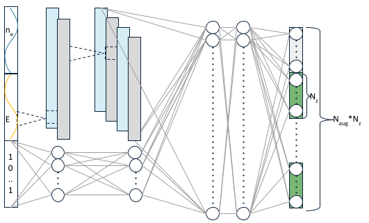
(a) Convolutional neural network architecture used in the amortized solver that maps simulation profiles onto a set of $n_{\mathrm{aug}}\,$ augmentation vectors $v_{1},\ldots\,v_{n_{\mathrm{aug}}\,}$.

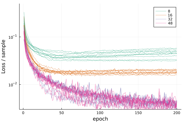
(b) Loss over the test set, grouped by the number of augmentation vectors $n_{\mathrm{aug}}\,$ returned by the model.

Figure 1: Network architecture (left) and test losses (right)

A convolutional neural network, shown in Fig. 1(a), maps the electron density profile $n_{\mathrm{e}}\,(z)$, the Electric field $E(z)$ profile and a one-hot encoding of simulation parameters onto $\left\{v_{j}\right\}_{j=1}^{n_{\mathrm{aug}}\,}$. The profiles are concatenated and feed into two convolutional layers with $4$ and $16$ channels respectively. The one-hot encoded simulation parameters feed into two fully-connected MLP layers with $32$ neurons each. The output of these channels are flattened and merge into two fully-connected layers which are fed into the output layer of size $N_{z}\times n_{\mathrm{aug}}\,$. We train this network on data from a series of simulations where the initial positions of $32,768$ electrons is sampled from profiles of the form $n_{\mathrm{e}}\,(z,t=0)=A\cdot f(kz)$ with $A\in\{1,2,5,10\}\times 10^{-3}$, $f\in\left\{\sin,\cos\right\}$, $k\in\{1,2\}$. The initial positions of $32,768$ singly charged ions is sampled from a uniform distributions and both electrons and ions are initially cold. These initial conditions on the particles are chosen as to excite electron plasma oscillations. The fields are evaluated on a grid with $N_{z}=64$ and $L_{z}=4\pi$. These 16 reference simulations are advanced with a timestep of $\triangle t=1$ from $T=0$ to $T=30$. This yields $480$ training profiles.

Targeting only the first Newton iteration, the neural network is trained by minimizing the orthogonal projection of $\left\{\delta E^{k=1}\right\}$ over the vector space spanned by the model output, as described by Trivedi et al. [19]

$$\mathcal{L}=\operatorname*{arg\,min}_{\widehat{y}\in\mathrm{span}(v_{1}\,\ldots,v_{n_{\mathrm{aug}}\,})}\frac{\|\widehat{y}-\delta E^{k=1}\|_{2}}{\|\delta E^{k=1}\|_{2}}+\lambda\,\|\mathrm{triu}\left(V*V^{\mathrm{tr}}\right)\|_{2}.$$ (5)

To calculate the projection, the output of the model $V$ is subject to a $\mathrm{QR}$ factorization, $Q,R=\mathrm{qr}\left(V\right)$ [20] and the projection is calculated as $\widehat{y}=Q\cdot Q^{\prime}\cdot\delta E^{k=1}$. Additionally, the last term penalizes collinearity of output vectors. Here $\mathrm{triu}(A)=\left\{a_{r,s}\right\}_{r<s}$ denotes the upper triangular part of a square matrix and $V=\left[v_{1}|\ldots|v_{n_{\mathrm{aug}}\,}\right]$.

To identify optimal hyperparameters of the network, the $480$ profiles are split $80\%/20\%$ into a training set and a test set. The network is trained for 200 epochs to minimize Eq. 5 over the training set. We use ReLU, tanh, and swish [21] activation functions, vary the size of the convolution filters used in both convolutional layers, choosing from $\{3,5,7,9,13\}$, vary dropout probabilities in fully connected layers [22] over $\{0.1,0.2,0.3\}$, vary $\lambda\in\{10^{-3},10^{-4},10^{-5}\}$ vary the initial learning rate from $\{10^{-2},10^{-3},5\times 10^{-4}\}$, and use ADAM [23], RMSProp and SGD optimizers. Average loss over the test set serves as the metric to evaluate optimal hyperparameters. Figure 1(b) shows a sub-set of the training losses for various $n_{\mathrm{aug}}\,$, $\lambda$ and dropout probabilities. We observe that more augmentation vectors results in lower per-sample loss. Additionally we observe only little over-fitting for $n_{\mathrm{aug}}\,=8,16$. From this scan we identify ReLU activation functions, convolutional filters of width $3$, a Dropout probability of $0.2$, $\lambda=10^{-4}$, as ideal parameters and optimize using the ADAM algorithm with an initial learning rate of $0.001$. Training was performed on nVidia V100 GPUs, in less than 2 hours of total computation time, using the Flux library [24, 25]. Simulation data for training and inference was produced using this code . Instructions on how to generate the data are available from the author upon request.

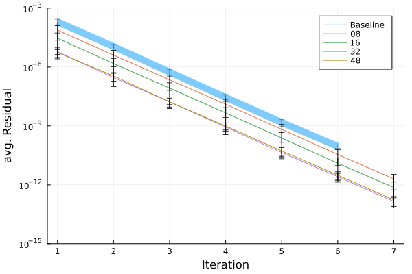
(a) $n_{\mathrm{e},t=0}(z)=10^{-2}\left[0.1\cos(2z)+0.9\sin(z)\right]$.

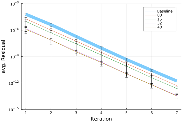
(b) $n_{\mathrm{e},t=0}(z)=3\times 10^{-3}\left[0.5\sin(z)+0.5\cos(2z)\right]$.

Figure 2: Residuals at various GMRES iterations of the original and amortized solver using $n_{\mathrm{aug}}\,\in\left\{8,16,32,48\right\}$, averaged over an entire simulation.

The performance of the trained amortized solver is evaluated on simulations where the initial positions of the electrons are sampled from $n_{\mathrm{e},t=0}(z)=A\left[a_{1}f_{1}(k_{1}z)+a_{2}f_{2}(k_{2}z)\right]$. Ions are again sampled from a uniform distribution and both particles are cold. Initial profile parameters are chosen as $f_{1},f_{2}\in\left\{\sin,\cos\right\}$, $k_{1},k_{2}\in\left\{1,2\right\}$. Figures 2(a) and 2(b) show the residual at each GMRES iteration in the these simulation, averaged over all 30 timesteps. The thick blue lines denote residuals observed in simulations using a plain GMRES solver and the thin, colored lines show residuals observed when using the trained amortized for $n_{\mathrm{aug}}\,=8,16,32,48$. Using $n_{\mathrm{aug}}\,=8$ the average residuals of the amortized solver are only slightly smaller than those of plain GMRES. For $n_{\mathrm{aug}}\,=16$, the average residuals of the amortized solver are of the same magnitude as those of plain GMRES but after its following iteration ahead. That is, the amortized solver requires one less iteration to converge to the same tolerance as plain GMRES. For $n_{\mathrm{aug}}\,=32$ and $n_{\mathrm{aug}}\,=48$, the amortized solver requires two fewer iterations to converge the residual to the same tolerance as the plain GMRES.

In conclusion, we demonstrate the feasibility to accelerate plasma simulations using implicit PIC methods with a machine-learning based amortized solver. For simulations of electron plasma oscillations the number of required GMRES iterations per first Newton iteration may be reduced from about 7 to about 5. The fidelity of the accelerated simulations is unmodified and they retain all conservation properties. Future work will focus on re-formulating the amortized solver to make use of more direct Krylov space augmentation techniques as discussed for example in [13, 14, 19]. We hope to achieve a net speed-up of the simulations using such techniques. Finally, we aim to investigate how the performance of the amortized solver depends on the training set and explore performance for other types of simulations such as ion acoustic waves.

3 Acknowledgements

The simulations presented in this article were performed on computational resources managed and supported by Princeton Research Computing, a consortium of groups including the Princeton Institute for Computational Science and Engineering (PICSciE) and the Office of Information Technology’s High Performance Computing Center and Visualization Laboratory at Princeton University.

References

- Ku et al. [2016] S. Ku, R. Hager, C.S. Chang, J.M. Kwon, and S.E. Parker. A new hybrid-lagrangian numerical scheme for gyrokinetic simulation of tokamak edge plasma. Journal of Computational Physics, 315:467–475, 2016. ISSN 0021-9991. doi: https://doi.org/10.1016/j.jcp.2016.03.062. URL https://www.sciencedirect.com/science/article/pii/S0021999116300274.
- Chang et al. [2017] C. S. Chang, S. Ku, G. R. Tynan, R. Hager, R. M. Churchill, I. Cziegler, M. Greenwald, A. E. Hubbard, and J. W. Hughes. Fast low-to-high confinement mode bifurcation dynamics in a tokamak edge plasma gyrokinetic simulation. Phys. Rev. Lett., 118:175001, Apr 2017. doi: 10.1103/PhysRevLett.118.175001. URL https://link.aps.org/doi/10.1103/PhysRevLett.118.175001.
- Ku et al. [2018] S. Ku, C. S. Chang, R. Hager, R. M. Churchill, G. R. Tynan, I. Cziegler, M. Greenwald, J. Hughes, S. E. Parker, M. F. Adams, E. D’Azevedo, and P. Worley. A fast low-to-high confinement mode bifurcation dynamics in the boundary-plasma gyrokinetic code xgc1. Physics of Plasmas, 25(5):056107, 2018. doi: 10.1063/1.5020792. URL https://doi.org/10.1063/1.5020792.
- Hager et al. [2020] R. Hager, C. S. Chang, N. M. Ferraro, and R. Nazikian. Gyrokinetic understanding of the edge pedestal transport driven by resonant magnetic perturbations in a realistic divertor geometry. Physics of Plasmas, 27(6):062301, 2020. doi: 10.1063/1.5144445. URL https://doi.org/10.1063/1.5144445.
- Wang et al. [2019] Bei Wang, Stephane Ethier, William Tang, Khaled Z Ibrahim, Kamesh Madduri, Samuel Williams, and Leonid Oliker. Modern gyrokinetic particle-in-cell simulation of fusion plasmas on top supercomputers. The International Journal of High Performance Computing Applications, 33(1):169–188, 2019. doi: 10.1177/1094342017712059. URL https://doi.org/10.1177/1094342017712059.
- Chien et al. [2020] Steven W. D. Chien, Jonas Nylund, Gabriel Bengtsson, Ivy B. Peng, Artur Podobas, and Stefano Markidis. sputnipic: An implicit particle-in-cell code for multi-gpu systems. In 2020 IEEE 32nd International Symposium on Computer Architecture and High Performance Computing (SBAC-PAD), pages 149–156, 2020. doi: 10.1109/SBAC-PAD49847.2020.00030.
- Bird et al. [2021] Robert F. Bird, Nigel Tan, Scott V. Luedtke, Stephen Lien Harrell, Michela Taufer, and Brian J. Albright. VPIC 2.0: Next generation particle-in-cell simulations. CoRR, abs/2102.13133, 2021. URL https://arxiv.org/abs/2102.13133.
- Ohana et al. [2021] Noé Ohana, Claudio Gheller, Emmanuel Lanti, Andreas Jocksch, Stephan Brunner, and Laurent Villard. Gyrokinetic simulations on many- and multi-core architectures with the global electromagnetic particle-in-cell code orb5. Computer Physics Communications, 262:107208, 2021. ISSN 0010-4655. doi: https://doi.org/10.1016/j.cpc.2020.107208. URL https://www.sciencedirect.com/science/article/pii/S0010465520300461.
- Mniszewski et al. [2021] Susan M Mniszewski, James Belak, Jean-Luc Fattebert, Christian FA Negre, Stuart R Slattery, Adetokunbo A Adedoyin, Robert F Bird, Choongseok Chang, Guangye Chen, Stéphane Ethier, Shane Fogerty, Salman Habib, Christoph Junghans, Damien Lebrun-Grandié, Jamaludin Mohd-Yusof, Stan G Moore, Daniel Osei-Kuffuor, Steven J Plimpton, Adrian Pope, Samuel Temple Reeve, Lee Ricketson, Aaron Scheinberg, Amil Y Sharma, and Michael E Wall. Enabling particle applications for exascale computing platforms. The International Journal of High Performance Computing Applications, 0(0):10943420211022829, 2021. doi: 10.1177/10943420211022829. URL https://doi.org/10.1177/10943420211022829.
- Chen et al. [2011] G. Chen, L. Chacón, and D.C. Barnes. An energy- and charge-conserving, implicit, electrostatic particle-in-cell algorithm. Journal of Computational Physics, 230(18):7018–7036, 2011. ISSN 0021-9991. doi: https://doi.org/10.1016/j.jcp.2011.05.031. URL https://www.sciencedirect.com/science/article/pii/S0021999111003421.
- Chen et al. [2014] G. Chen, L. Chacón, C.A. Leibs, D.A. Knoll, and W. Taitano. Fluid preconditioning for newton–krylov-based, fully implicit, electrostatic particle-in-cell simulations. Journal of Computational Physics, 258:555–567, 2014. ISSN 0021-9991. doi: https://doi.org/10.1016/j.jcp.2013.10.052. URL https://www.sciencedirect.com/science/article/pii/S0021999113007286.
- Sturdevant et al. [2021] Benjamin J. Sturdevant, S. Ku, L. Chacón, Y. Chen, D. Hatch, M. D. J. Cole, A. Y. Sharma, M. F. Adams, C. S. Chang, S. E. Parker, and R. Hager. Verification of a fully implicit particle-in-cell method for the v||-formalism of electromagnetic gyrokinetics in the xgc code. Physics of Plasmas, 28(7):072505, 2021. doi: 10.1063/5.0047842. URL https://doi.org/10.1063/5.0047842.
- Morgan [1995] Ronald B. Morgan. A restarted gmres method augmented with eigenvectors. SIAM Journal on Matrix Analysis and Applications, 16(4):1154–1171, 1995. doi: 10.1137/S0895479893253975. URL https://doi.org/10.1137/S0895479893253975.
- Chapman and Saad [1997] Andrew Chapman and Yousef Saad. Deflated and augmented krylov subspace techniques. In Numerical Linear Algebra with Applications, volume 4, pages 43–66. John Wiley & Sons, Ltd, 2021/09/20 1997. ISBN 1070-5325. doi: https://doi.org/10.1002/(SICI)1099-1506(199701/02)4:1<43::AID-NLA99>3.0.CO;2-Z. URL https://doi.org/10.1002/(SICI)1099-1506(199701/02)4:1<43::AID-NLA99>3.0.CO;2-Z.
- Gaul [2014] André Gaul. Recycling Krylov subspace methods for sequences of linear systems : Analysis and applications. Doctoral thesis, Technische Universität Berlin, Fakultät II - Mathematik und Naturwissenschaften, Berlin, 2014. URL http://dx.doi.org/10.14279/depositonce-4147.
- Raissi et al. [2019] M. Raissi, P. Perdikaris, and G.E. Karniadakis. Physics-informed neural networks: A deep learning framework for solving forward and inverse problems involving nonlinear partial differential equations. Journal of Computational Physics, 378:686–707, 2019. ISSN 0021-9991. doi: https://doi.org/10.1016/j.jcp.2018.10.045. URL https://www.sciencedirect.com/science/article/pii/S0021999118307125.
- Pathak et al. [2020] Jaideep Pathak, Mustafa Mustafa, Karthik Kashinath, Emmanuel Motheau, Thorsten Kurth, and Marcus Day. Using machine learning to augment coarse-grid computational fluid dynamics simulations, 2020.
- Kochkov et al. [2021] Dmitrii Kochkov, Jamie A. Smith, Ayya Alieva, Qing Wang, Michael P. Brenner, and Stephan Hoyer. Machine learning–accelerated computational fluid dynamics. Proceedings of the National Academy of Sciences, 118(21), 2021. ISSN 0027-8424. doi: 10.1073/pnas.2101784118. URL https://www.pnas.org/content/118/21/e2101784118.
- Trivedi et al. [2019] Rahul Trivedi, Logan Su, Jesse Lu, Martin F. Schubert, and Jelena Vuckovic. Data-driven acceleration of photonic simulations. Scientific Reports, 9(1):19728, 2019. doi: 10.1038/s41598-019-56212-5. URL https://doi.org/10.1038/s41598-019-56212-5.
- Seeger et al. [2017] Matthias W. Seeger, Asmus Hetzel, Zhenwen Dai, and Neil D. Lawrence. Auto-differentiating linear algebra. CoRR, abs/1710.08717, 2017. URL http://arxiv.org/abs/1710.08717.
- Ramachandran et al. [2017] Prajit Ramachandran, Barret Zoph, and Quoc V. Le. Searching for activation functions. CoRR, abs/1710.05941, 2017. URL http://arxiv.org/abs/1710.05941.
- Srivastava et al. [2014] Nitish Srivastava, Geoffrey Hinton, Alex Krizhevsky, Ilya Sutskever, and Ruslan Salakhutdinov. Dropout: A simple way to prevent neural networks from overfitting. Journal of Machine Learning Research, 15(56):1929–1958, 2014. URL http://jmlr.org/papers/v15/srivastava14a.html.
- Kingma and Ba [2017] Diederik P. Kingma and Jimmy Ba. Adam: A method for stochastic optimization, 2017.
- Innes et al. [2018] Michael Innes, Elliot Saba, Keno Fischer, Dhairya Gandhi, Marco Concetto Rudilosso, Neethu Mariya Joy, Tejan Karmali, Avik Pal, and Viral Shah. Fashionable modelling with flux. CoRR, abs/1811.01457, 2018. URL https://arxiv.org/abs/1811.01457.
- Innes [2018] Mike Innes. Flux: Elegant machine learning with julia. Journal of Open Source Software, 2018. doi: 10.21105/joss.00602.