Energy partition between Alfvénic and compressive fluctuations in magnetorotational turbulence with near-azimuthal mean magnetic field

Abstract

The theory of magnetohydrodynamic (MHD) turbulence predicts that Alfvénic and slow-mode-like compressive fluctuations are energetically decoupled at small scales in the inertial range. The partition of energy between these fluctuations determines the nature of dissipation, which, in many astrophysical systems, happens on scales where plasma is collisionless. However, when the magnetorotational instability (MRI) drives the turbulence, it is difficult to resolve numerically the scale at which both types of fluctuations start to be decoupled because the MRI energy injection occurs in a broad range of wavenumbers, and both types of fluctuations are usually expected to be coupled even at relatively small scales. In this study, we focus on collisional MRI turbulence threaded by a near-azimuthal mean magnetic field, which is naturally produced by the differential rotation of a disc. We show that, in such a case, the decoupling scales are reachable using a reduced MHD model that includes differential-rotation effects. In our reduced MHD model, the Alfvénic and compressive fluctuations are coupled only through the linear terms that are proportional to the angular velocity of the accretion disc. We numerically solve for the turbulence in this model and show that the Alfvénic and compressive fluctuations are decoupled at the small scales of our simulations as the nonlinear energy transfer dominates the linear coupling below the MRI-injection scale. In the decoupling scales, the energy flux of compressive fluctuations contained in the small scales is almost double that of Alfvénic fluctuations. Finally, we discuss the application of this result to prescriptions of ion-to-electron heating ratio in hot accretion flows.

1 Introduction

Accretion of matter onto a central massive object is one of the most spectacular astronomical phenomena. A number of theoretical and numerical studies of accretion flows have been conducted for decades (see Balbus & Hawley, 1998; Lesur, 2021, and references therein), including the discovery of momentum transport due to turbulence driven by magnetorotational instability (MRI; Balbus & Hawley, 1991). On the observational front, the Event Horizon Telescope (EHT) successfully captured an image of a radiating disc at M87 (EHT Collaboration, 2019), opening the door to direct comparisons between models and observations. However, there are many unsolved questions in MRI-driven turbulence that are crucial for interpreting such observations. In this study, we focus on the energy partition between Alfvénic and slow-mode-like compressive fluctuations in collisional MRI turbulence. This is important in deciding the partition of heating between ions and electrons at dissipation scales, where plasma is collisionless (Kawazura et al., 2020).

In order to calculate the partition of energy between Alfvénic and compressive fluctuations in a numerical simulation, one must access scales small enough that these fluctuations become energetically decoupled. It is known that such decoupling is established at the scale where the reduced magnetohydrodynamics (RMHD) approximation, $k_{\|}/k_{\perp}\ll 1$ and $|\delta{\boldsymbol{\mathrm{B}}}|/B_{0}\sim|\delta{\boldsymbol{\mathrm{u}}}|/v_{\mathrm{A}}\ll 1$, is satisfied (Schekochihin et al., 2009). Here, the subscript $\|$ (${\perp}$) denotes the component parallel (perpendicular) to the ambient magnetic field, the prefix $\delta$ and the subscript 0 denote the fluctuation and equilibrium fields, respectively, and $v_{\mathrm{A}}$ denotes the Alfvén speed. The RMHD approximation is expected to be satisfied at sufficiently small scales in the inertial range, because the large-scale magnetic field serves as an effective mean field for the fluctuations at the smaller scales (Kraichnan, 1965). Once the cascade reaches the RMHD range, the partition of Alfvénic and compressive fluctuations is maintained down to the ion Larmor scale (Schekochihin et al., 2009).

While the partition of Alfvénic and compressive fluctuations has been studied in externally forced MHD turbulence (Cho & Lazarian, 2002, 2003; Makwana & Yan, 2020), none of the previous studies of MRI turbulence have investigated this problem. Previous MRI turbulence simulations have suggested that, in order to reach the RMHD range, significantly higher numerical resolution is necessary for MRI turbulence than for externally forced MHD turbulence, because there is non-local energy transfer (Lesur & Longaretti, 2011), meaning that the injection range is broad in the Fourier space.

Here, instead of carrying out brute-force high-resolution MHD simulations, we study the partition of Alfvénic and compressive fluctuations by reducing the MHD equations to a more tractable form that is valid only when there is a mean magnetic field in approximately azimuthal direction. The presence of the near-azimuthal mean magnetic field is a natural consequence of the differential rotation of the disc; even when the system is initialized with a purely vertical magnetic field, MRI creates a radial magnetic field which will then be twisted in the azimuthal direction. Indeed, predominantly azimuthal magnetic field is quite often seen both in local and global simulations of MRI turbulence (e.g., Suzuki & Inutsuka, 2009, 2014). A statistical analysis of MRI turbulence in incompressible MHD also supports the presence of a near-azimuthal mean field (Zhdankin et al., 2017). We show that the RMHD approximation captures the fastest-growing MRI modes in such a system. We then simulate this type of MRI turbulence numerically and show that the compressive fluctuations carry almost twice as much energy flux as Alfvénic fluctuations at the small scales, where the two kinds of fluctuations are decoupled.

2 Model

We consider a local shearing-box approximation (Goldreich & Lynden-Bell, 1965) for a plasma in Cartesian coordinates $(X,\,Y,\,Z)$ located at a fixed radius $r=r_{0}$ and rotating with an angular velocity ${\boldsymbol{\mathrm{\Omega}}}=\Omega\hat{{\boldsymbol{\mathrm{Z}}}}$, where $X$, $Y$, and $Z$ correspond to the radial, azimuthal, and vertical (rotation-axis) directions. The MHD equations in these conditions are

$$\frac{\p\rho}{\p t}+{\boldsymbol{\mathrm{u}}}\cdot\nabla\rho+{\boldsymbol{\mathrm{u}}}_{0}\cdot\nabla\rho=-\rho(\nabla\cdot{\boldsymbol{\mathrm{u}}}),$$ (1a)

$$\rho\left(\frac{\p}{\p t}+{\boldsymbol{\mathrm{u}}}\cdot\nabla+{\boldsymbol{\mathrm{u}}}_{0}\cdot\nabla\right){\boldsymbol{\mathrm{u}}}=-\nabla\left(p+\frac{B^{2}}{8\pi}\right)+\frac{{\boldsymbol{\mathrm{B}}}\cdot\nabla{\boldsymbol{\mathrm{B}}}}{4\pi}-2\rho{\boldsymbol{\mathrm{\Omega}}}\times{\boldsymbol{\mathrm{u}}}-\rho{\boldsymbol{\mathrm{u}}}\cdot\nabla{\boldsymbol{\mathrm{u}}}_{0},$$ (1b)

$$\frac{\p{\boldsymbol{\mathrm{B}}}}{\p t}+{\boldsymbol{\mathrm{u}}}\cdot\nabla{\boldsymbol{\mathrm{B}}}+{\boldsymbol{\mathrm{u}}}_{0}\cdot\nabla{\boldsymbol{\mathrm{B}}}+{\boldsymbol{\mathrm{B}}}(\nabla\cdot{\boldsymbol{\mathrm{u}}})={\boldsymbol{\mathrm{B}}}\cdot\nabla{\boldsymbol{\mathrm{u}}}+{\boldsymbol{\mathrm{B}}}\cdot\nabla{\boldsymbol{\mathrm{u}}}_{0},$$ (1c)

$$\frac{\p p}{\p t}+{\boldsymbol{\mathrm{u}}}\cdot\nabla p+{\boldsymbol{\mathrm{u}}}_{0}\cdot\nabla p+\Gamma p\nabla\cdot{\boldsymbol{\mathrm{u}}}=0,$$ (1d)

where $\rho$ is the mass density, ${\boldsymbol{\mathrm{u}}}$ is the fluid velocity, ${\boldsymbol{\mathrm{B}}}$ is the magnetic field, $p$ is the thermal pressure, ${\boldsymbol{\mathrm{u}}}_{0}\equiv q{\boldsymbol{\mathrm{X}}}\times{\boldsymbol{\mathrm{\Omega}}}$ is the background shear flow, $q$ is a shear rate, and $\Gamma=5/3$ is the specific heat ratio. Hereafter, we only consider Keplerian rotation ($q=3/2$) and call (1a)-(1d) the “full-MHD” equations.

Balbus & Hawley (1992b) showed that the fastest-growing MRI modes have $k_{Z}\to\infty$ when the ambient magnetic field ${\boldsymbol{\mathrm{B}}}_{0}$ approaches the azimuthal direction. These fastest-growing modes also satisfy $k_{\|}v_{\mathrm{A}}/\Omega\simeq 1$. For a near-azimuthal ${\boldsymbol{\mathrm{B}}}_{0}$, $\hat{{\boldsymbol{\mathrm{Z}}}}$ is almost perpendicular to ${\boldsymbol{\mathrm{B}}}_{0}$, meaning that the fastest growing modes satisfy $k_{\|}/k_{\perp}\ll 1$. Therefore, if the fastest-growing modes decide the nature of MRI turbulence at the smaller scales, we can ignore the scales that are outside of the $k_{\|}/k_{\perp}\ll 1$ approximation. This idea motivates us to impose the RMHD approximation on the full-MHD equations (1a)-(1d). We assume also that the magnetic perturbations are separated from the time-invariant and spatially uniform mean fields as ${\boldsymbol{\mathrm{B}}}={\boldsymbol{\mathrm{B}}}_{0}+\delta{\boldsymbol{\mathrm{B}}}$, where ${\boldsymbol{\mathrm{B}}}_{0}$ is taken to have finite $Y$ (azimuthal) and $Z$ (vertical) components but no $X$ (radial) component. We assume that the density and pressure are also separated into a constant background and perturbations as $\rho=\rho_{0}+\delta\!\rho$ and $p=p_{0}+\delta\!p$. The angle between $\hat{{\boldsymbol{\mathrm{Y}}}}$ and ${\boldsymbol{\mathrm{B}}}_{0}$ is denoted by $\theta\;[0\leq\theta\leq\pi;\text{the same definition as \cite[citet]{\@@bibref{Authors Phrase1YearPhrase2}{Quataert2002}{\@@citephrase{(}}{\@@citephrase{)}}}}]$. In this study, we focus on the near-azimuthal background field, i.e., $\sin\theta\ll 1$. Then, we introduce a “tilted” coordinate set $(x,\,y,\,z)$ in which the $z$-axis is aligned with ${\boldsymbol{\mathrm{B}}}_{0}$, and the $x$-axis is aligned with the $X$-axis (Fig. 1), i.e., $(x,y,z)$ is a rotation of $(X,Y,Z)$ by $\pi/2-\theta$ about the $\hat{{\boldsymbol{\mathrm{X}}}}$ axis. When $\sin\theta\ll 1$, $\hat{{\boldsymbol{\mathrm{z}}}}$ and $\hat{{\boldsymbol{\mathrm{y}}}}$ almost align with $\hat{{\boldsymbol{\mathrm{Y}}}}$ and $-\hat{{\boldsymbol{\mathrm{Z}}}}$, respectively. This tilted coordinate set is more convenient than the standard coordinate set $(X,\,Y,\,Z)$ because $k_{z}\sim k_{\|}\ll k_{\perp}$ is a key criterion for the decoupling of Alfvénic and compressive fluctuations. In the standard coordinate set, however, $k_{\|}$ and $k_{\perp}$ are more difficult to separate, both being a mixture of $k_{Y}$ and $k_{Z}$.

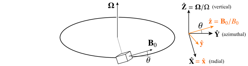
Figure 1: Schematic of the conventional coordinate system $(X,Y,Z)$ and our tilted coordinate system $(x,y,z)$.

Thus, we impose the RMHD ordering $k_{\|}\ll k_{\perp},\,{\boldsymbol{\mathrm{u}}}\ll v_{\mathrm{A}}$, and $\delta{\boldsymbol{\mathrm{B}}}\ll{\boldsymbol{\mathrm{B}}}_{0}$ on (1a)-(1d). We also assume $\p/\p t\sim\Omega\sim k_{\|}v_{\mathrm{A}}$ and a near-azimuthal ${\boldsymbol{\mathrm{B}}}_{0}$, i.e., $\sin\theta\ll 1$, with $\sin\theta$ the same order of smallness as $k_{\|}/k_{\perp}$ and $\delta\!B/B_{0}$. The assumed anisotropy between $k_{\|}$ and $k_{\perp}$ is motivated by the critical balance conjecture (CB; Goldreich & Sridhar, 1995, 1997):

$$k_{\|}v_{\mathrm{A}}\sim k_{\perp}u_{\perp},$$ (2)

which physically means that the time scales of linear wave propagation along ${\boldsymbol{\mathrm{B}}}_{0}$ and nonlinear cascade in the plane perpendicular to ${\boldsymbol{\mathrm{B}}}_{0}$ are of the same order. Then, we obtain the RMHD equations with differential rotation (see appendix A for the detailed derivation):

$$\frac{\mathrm{d}\Psi}{\mathrm{d}t}=v_{\mathrm{A}}\frac{\p\Phi}{\p z},$$ (3a)

$$\frac{\mathrm{d}}{\mathrm{d}t}\nabla_{\perp}^{2}\Phi=v_{\mathrm{A}}\nabla_{\|}\nabla_{\perp}^{2}\Psi-2\Omega\,\frac{\p u_{\|}}{\p y},$$ (3b)

$$\frac{\mathrm{d}u_{\|}}{\mathrm{d}t}=v_{\mathrm{A}}^{2}\nabla_{\|}\frac{\delta\!B_{\|}}{B_{0}}+(2-q)\Omega\,\frac{\p\Phi}{\p y},$$ (3c)

$$\frac{\mathrm{d}}{\mathrm{d}t}\left(1+\frac{v_{\mathrm{A}}^{2}}{c_{\mathrm{S}}^{2}}\right)\frac{\delta\!B_{\|}}{B_{0}}=\nabla_{\|}u_{\|}+\frac{q\Omega}{v_{\mathrm{A}}}\,\frac{\p\Psi}{\p y},$$ (3d)

where $c_{\mathrm{S}}$ is the sound speed, and $\Phi$ and $\Psi$ are the stream function and magnetic flux function defined by ${\boldsymbol{\mathrm{u}}}_{\perp}=\hat{{\boldsymbol{\mathrm{z}}}}\times\nabla_{\perp}\Phi$ and $\delta{\boldsymbol{\mathrm{B}}}_{\perp}=\sqrt{4\pi\rho_{0}}\hat{{\boldsymbol{\mathrm{z}}}}\times\nabla_{\perp}\Psi$, respectively. We have also defined $\mathrm{d}/\mathrm{d}t\equiv\p/\p t+{\boldsymbol{\mathrm{u}}}_{\perp}\cdot\nabla_{\perp}$ and $\nabla_{\|}\equiv\p/\p z+(\delta{\boldsymbol{\mathrm{B}}}_{\perp}/B_{0})\cdot\nabla_{\perp}$. Hereafter, we call these equations Rotating RMHD (RRMHD). When $\Omega=0$, these become the standard RMHD equations (Kadomtsev & Pogutse, 1974; Strauss, 1976), which is a long-wavelength limit of gyrokinetics and in which Alfvénic and compressive fluctuations are decoupled (Schekochihin et al., 2009).

One may notice that (3a)-(3d) do not have the shearing effect that originates from ${\boldsymbol{\mathrm{u}}}_{0}\cdot\nabla$ terms in (1a)-(1d). This is due to $k_{\|}/k_{\perp}\ll 1$ and $\sin\theta\ll 1$; in a shearing box, the radial wavenumber depends on time as $k_{x}(t)=k_{x}(0)+q\Omega t(k_{y}\sin\theta+k_{\|}\cos\theta)$ [see, e.g., the fourth term in the left-hand side of (16)], and the time-dependent term on the right-hand side is ordered out because $\sin\theta\sim k_{\|}/k_{x}(0)\sim\epsilon$. However, when we consider a long-time evolution $\Omega t\sim\epsilon^{-1}$, the time dependence is not negligible. In that case, the non-modal growth of MRI (Squire & Bhattacharjee, 2014a, b) becomes important. On the other hand, as we will show below, the eddy turnover time in RRMHD turbulence gets shorter than the disc rotation time, i.e., $k_{\perp}u_{\perp}/\Omega\gg 1$ immediately below the injection scale (see Fig. 7). Therefore, we do not need to consider a long-time evolution with $\Omega t\sim\epsilon^{-1}$.

As we shall see in the next section, when $\Omega\neq 0$, this system can be MRI unstable. In the turbulent state, the magnitudes of the nonlinear terms in (3a)-(3d) increase as the cascade proceeds to smaller scales, and at some point, the linear terms that are proportional to $\Omega$ become negligible. Below the scale at which this happens, the turbulence is governed by standard RMHD, and thus Alfvénic and compressive fluctuations are decoupled. As we will see below, this critical scale roughly corresponds to the scale at which the eddy turnover time becomes shorter than $\Omega^{-1}$. In other words, when an eddy’s lifetime is much shorter than the orbital time of the disc, the effects of the disc’s rotation are insignificant. Therefore, the transient growth effects (Balbus & Hawley, 1992a; Mamatsashvili et al., 2013) are absent. We also note that, with the normalizations $t\Omega\to t$, $z\Omega/v_{\mathrm{A}}\to z$, $x/L_{\perp}\to x$, $\Phi/L_{\perp}^{2}\Omega\to\Phi$, $\Psi/L_{\perp}^{2}\Omega\to\Psi$, $u_{\|}/L_{\perp}\Omega\to u_{\|}$, and $v_{\mathrm{A}}\delta\!B_{\|}/B_{0}L_{\perp}\Omega\to\delta\!B_{\|}$, the rotation rate is no longer a free parameter, and the only remaining parameter is $c_{\mathrm{S}}^{2}/v_{\mathrm{A}}^{2}=\Gamma\beta/2$, where $\beta=8\pi p_{0}/B_{0}^{2}$.

The nonlinear free-energy invariant of (3a)-(3d) consists of Alfvénic and compressive portions $W_{\mathrm{tot}}=W_{\mathrm{AW}}+W_{\mathrm{compr}}$, where

$$W_{\mathrm{AW}} =\frac{1}{2}\int\mathrm{d}^{3}{\boldsymbol{\mathrm{r}}}\left[|\nabla_{\perp}\Phi|^{2}+|\nabla_{\perp}\Psi|^{2}\right],$$ (4a)

$$W_{\mathrm{compr}} =\frac{1}{2}\int\mathrm{d}^{3}{\boldsymbol{\mathrm{r}}}\left[u_{\|}^{2}+v_{\mathrm{A}}^{2}\left(1+\frac{v_{\mathrm{A}}^{2}}{c_{\mathrm{S}}^{2}}\right)\frac{\delta\!B_{\|}^{2}}{B_{0}^{2}}\right].$$ (4b)

The time evolution of $W_{\mathrm{AW}}$ and $W_{\mathrm{compr}}$ is given by

$$\frac{\mathrm{d}W_{\mathrm{AW}}}{\mathrm{d}t} =-2\Omega\int\mathrm{d}^{3}{\boldsymbol{\mathrm{r}}}\,u_{\|}\frac{\p\Phi}{\p y}\equiv I_{\mathrm{AW}},$$ (5a)

$$\frac{\mathrm{d}W_{\mathrm{compr}}}{\mathrm{d}t} =q\Omega\int\mathrm{d}^{3}{\boldsymbol{\mathrm{r}}}\,\left[v_{\mathrm{A}}\frac{\delta\!B_{\|}}{B_{0}}\frac{\p\Psi}{\p y}-u_{\|}\frac{\p\Phi}{\p y}\right]+2\Omega\int\mathrm{d}^{3}{\boldsymbol{\mathrm{r}}}\,u_{\|}\frac{\p\Phi}{\p y}\equiv I_{\mathrm{compr}},$$ (5b)

where $I_{\mathrm{AW}}$ and $I_{\mathrm{compr}}$ are the energy injection rates of Alfvénic and compressive fluctuations. Noticing that the second term of $I_{\mathrm{compr}}$ is identical to $-I_{\mathrm{AW}}$, we may write $I_{\mathrm{compr}}=I_{\mathrm{MRI}}-I_{\mathrm{AW}}$. Then the net injection rate by the MRI is $I_{\mathrm{MRI}}$, and it goes into compressive fluctuations, which then exchange energy with Alfvénic fluctuations at the rate $I_{\mathrm{AW}}$ via linear coupling.

3 Linear MRI of RRMHD

Next, we compare the linear MRI growth rate of full-MHD and RRMHD to show that RRMHD can capture the MRI growth rate of full-MHD when ${\boldsymbol{\mathrm{B}}}_{0}$ is nearly azimuthal, viz., $\sin\theta\ll 1$. Here, we focus on the modes that are symmetric with respect to the rotation axis $\hat{{\boldsymbol{\mathrm{Z}}}}$, viz., $k_{Y}=0$, which is equivalent to $k_{y}=-k_{z}/\tan\theta$. We focus on these modes because they are the fastest growing ones. The linear dispersion relation of full-MHD (Balbus & Hawley, 1998, Eq. 99) is

$$\left[\omega^{2}-(k_{\|}v_{\mathrm{A}})^{2}\right]\left\{\omega^{4}-\left[k_{x}^{2}+(k_{\|}/\sin\theta)^{2}\right](c_{\mathrm{S}}^{2}+v_{\mathrm{A}}^{2})\omega^{2}+(k_{\|}v_{\mathrm{A}})^{2}\left[k_{x}^{2}+(k_{\|}/\sin\theta)^{2}\right]c_{\mathrm{S}}^{2}\right\}\\ =2\left\{(2-q)\omega^{4}-k_{\|}^{2}\left[2c_{\mathrm{S}}^{2}+(2\cos^{2}\theta-q)(c_{\mathrm{S}}^{2}+v_{\mathrm{A}}^{2})/\sin^{2}\theta\right]\omega^{2}-qc_{\mathrm{S}}^{2}v_{\mathrm{A}}^{2}k_{\|}^{4}/\sin^{2}\theta\right\}\Omega^{2}.$$ (6)

On the other hand, the dispersion relation of RRMHD, (3a)-(3d), is

$$\left[\omega^{2}-(k_{\|}v_{\mathrm{A}})^{2}\right]\left[\left(1+\frac{v_{\mathrm{A}}^{2}}{c_{\mathrm{S}}^{2}}\right)\omega^{2}-(k_{\|}v_{\mathrm{A}})^{2}\right]=2\left[(2-q)\left(1+\frac{v_{\mathrm{A}}^{2}}{c_{\mathrm{S}}^{2}}\right)\omega^{2}+q(k_{\|}v_{\mathrm{A}})^{2}\right]\frac{k_{y}^{2}}{k_{\perp}^{2}}\Omega^{2}.$$ (7)

One can show that for both (6) and (7), $k_{x}=0$ gives the fastest-growing mode. For the RRMHD dispersion relation (7), the growth rate does not depend on $k_{y}$ when $k_{x}=0$. When $\Omega=0$, (6) recovers the Alfvén, slow, and fast modes, while (7) recovers the Alfvén and slow modes (the fast mode is eliminated in the RMHD ordering). The maximum growth rate of RRMHD is given by

$$\frac{\gamma_{\mathrm{max}}}{\Omega}=\sqrt{\frac{5}{18}\beta\left[20\beta+15-\sqrt{8(50\beta^{2}+75\beta+18})\right]},$$ (8)

where we have used $q=3/2$ and $\Gamma=5/3$. One finds that $\gamma_{\mathrm{max}}$ is an increasing function of $\beta$ ranging from $\gamma_{\mathrm{max}}/\Omega\to 0$ for $\beta\to 0$ to $\gamma_{\mathrm{max}}/\Omega\to 3/4$ for $\beta\to\infty$. Note that the high-$\beta$ limit of the maximum growth rate in RRMHD is the same as in full-MHD (Balbus & Hawley, 1998, Eq. 114), and the stabilization of MRI at $\beta\to 0$ is consistent with the study by Kim & Ostriker (2000), who found that MRI in full-MHD was stabilized when $\beta\to 0$ and $\theta<30^{\circ}$.

In Fig. 2, we compare the solutions to (6) and (7). Figure 2(a) shows the growth rate obtained with RRMHD for different values of $\beta$; one finds that $\gamma_{\mathrm{max}}$ of RRMHD decreases as $\beta$ decreases as expected from (8). Figures 2(b)-(d) show the growth rate obtained with full-MHD for different values of $\beta$ and $\theta$. For full-MHD, the growth rate does not depend on $\beta$ when $\theta=\pi/2$; however, when $\sin\theta\ll 1$, the growth rate decreases as $\beta$ decreases. Clearly, the growth rates in RRMHD match those in full-MHD with $\sin\theta\ll 1$, meaning that RRMHD captures the fastest-growing MRI modes when ${\boldsymbol{\mathrm{B}}}_{0}$ is nearly azimuthal.

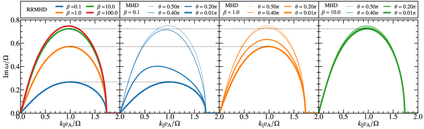
Figure 2: The linear MRI growth rate of (a) RRMHD and (b)-(d) full-MHD. The line colours correspond to the values of $\beta$ as given in the legend of (a). The line thickness for (b)-(d) corresponds to the value of $\theta$ as given in the legends of these panels. The horizontal dotted lines indicate that, independently of $\beta$, the maximum growth rates in RRMHD coincide with those in full-MHD in the limit of $\theta\to 0$.

4 Simulation of MRI turbulence in RRMHD

Next, we carry out nonlinear simulations of the RRMHD equations to compute the energy partition between the Alfvénic and compressive fluctuations in the saturated state of MRI turbulence. We solve (3a)-(3d) using a 3D pseudo-spectral code Calliope (Kawazura, 2022). In order to terminate the energy cascade at small scales, we add hyper-viscous and hyper-resistive terms proportional to $k_{\perp}^{8}$ and $k_{z}^{8}$ to the right-hand sides of (3a)-(3d). As mentioned above, the Alfvénic and compressive fluctuations are expected to be decoupled below some critical scale where the nonlinear terms start to dominate the linear terms. We set the computational grids so that this critical scale is well resolved, which we confirm later in this section. Therefore, the dissipation caused by the hyper-viscosity and hyper-resistivity in (3a) and (3b) is a measure of the energy flux carried by the Alfvénic fluctuations. Likewise, we can measure the energy flux carried by compressive fluctuations via the hyper-dissipation in (3c) and (3d). We denote the dissipation rates of the Alfvénic and compressive fluctuations by $D_{\mathrm{AW}}$ and $D_{\mathrm{compr}}$, respectively. The power balance of the system is then

$$\frac{\mathrm{d}W_{\mathrm{tot}}}{\mathrm{d}t}=I_{\mathrm{AW}}+I_{\mathrm{compr}}-D_{\mathrm{AW}}-D_{\mathrm{compr}}.$$ (9)

In a statistically stationary state, $\langle I_{\mathrm{AW}}\rangle+\langle I_{\mathrm{compr}}\rangle=\langle D_{\mathrm{AW}}\rangle+\langle D_{\mathrm{compr}}\rangle$, where $\langle\cdots\rangle$ denotes the time average. We set the box size of the simulations as $(L_{x},L_{y},L_{z})=(8\pi L_{\perp},2\pi L_{\perp},8\pi v_{\mathrm{A}}/\Omega)$ which is discretized by “low-resolution grids” $(n_{x},\,n_{y},\,n_{z})=(512,\,128,\,512)$, “medium-resolution grids” $(n_{x},\,n_{y},\,n_{z})=(1024,\,256,\,1024)$, and “high-resolution grids” $(n_{x},\,n_{y},\,n_{z})=(1024,\,256,\,2048)$. We choose $L_{z}$ so that the fastest-growing mode ($k_{z}v_{\mathrm{A}}/\Omega\simeq 1$, as seen in Fig. 2) fits in the box. We investigate three cases: $\beta=0.1,1$, and $10$. For all of these values of $\beta$, we start the simulation with the low-resolution grids and run for a sufficiently long time in the nonlinearly saturated state until $\langle\mathrm{d}W_{\mathrm{tot}}/\mathrm{d}t\rangle\simeq 0$ is satisfied before restarting with the higher-resolution grids.

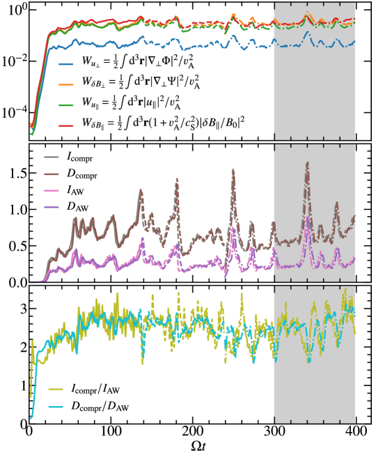
Figure 3: Time evolution of the $\beta=1$ run: (top) each component of the free energy (4a) and (4b) normalized by the total energy averaged over the nonlinearly saturated state, i.e., over the time interval $285\leq\Omega t\leq 330$; (middle) injection and dissipation rates of Alfvénic and compressive fluctuations normalized by the total injection power averaged over the nonlinearly saturated state; (bottom) the compressive-to-Alfvénic ratio of injection power $I_{\mathrm{compr}}/I_{\mathrm{AW}}$ and dissipation rate $D_{\mathrm{compr}}/D_{\mathrm{AW}}$. The solid, dashed, and dash-dotted lines correspond to the runs with the low-, medium-, and high-resolution grids, respectively. The shaded region indicates the interval used for the time averaging.

Figure 3 shows the time evolution of the free energy ($W_{\mathrm{AW}}$ and $W_{\mathrm{compr}}$), the power balance ($I_{\mathrm{AW}}$, $I_{\mathrm{compr}}$, $D_{\mathrm{AW}}$, $D_{\mathrm{compr}}$), the compressive-to-Alfvénic energy-injection ratio $I_{\mathrm{compr}}/I_{\mathrm{AW}}$, and the dissipation ratio $D_{\mathrm{compr}}/D_{\mathrm{AW}}$. From the top panel, one finds that the linear-growth phase occurs at $10\lesssim\Omega t\lesssim 20$ and is followed by the nonlinearly saturated turbulent phase. While the Alfvénic energy consists predominantly of $\delta\!B_{\perp}$, the compressive energy has almost the same contribution from $u_{\|}$ and $\delta\!B_{\|}$. We have confirmed that this trend is the same for $\beta=0.1$ and $10$. The middle panel shows that the energy injection balances with the energy dissipation. Interestingly, the amount of Alfvénic injection $I_{\mathrm{AW}}$ balances with Alfvénic dissipation $D_{\mathrm{AW}}$, and likewise, the compressive injection $I_{\mathrm{compr}}$ and dissipation $D_{\mathrm{compr}}$ are in balance. So, in the saturated state, there is, on average, barely any net nonlinear energy exchange between the two components of the turbulence – even at larger scales, where they are not formally decoupled. We have confirmed that this is also the case for $\beta=0.1$ and $10$. As we will see later, this may be due to the fact that the critical scale at which the Alfvénic and compressive fluctuations decouple is located close to the injection scale (see Figs. 6 and 7). The bottom panel shows the evolution of $I_{\mathrm{compr}}/I_{\mathrm{AW}}$ and $D_{\mathrm{compr}}/D_{\mathrm{AW}}$. One finds that both ratios are $\simeq 2-2.5$ in the nonlinear state. These values are almost the same for the runs with low-resolution grids (solid lines), medium-resolution grids (dashed lines), and high-resolution grids (dash-dotted lines).

Figure 4 shows snapshots of the turbulent fields. Structures are elongated in the $x$ direction, corresponding to the remnants of “channel flows” driven by MRI, also seen in other shearing-box simulations of full-MHD (e.g., Hawley & Balbus, 1992; Hirai et al., 2018). Note that our $\hat{{\boldsymbol{\mathrm{y}}}}$ direction is almost vertical within the accretion disc, $\hat{{\boldsymbol{\mathrm{y}}}}\simeq-{\boldsymbol{\mathrm{\Omega}}}/\Omega$ (see Fig. 1). For the Alfvénic fields, one finds that ${\boldsymbol{\mathrm{u}}}_{\perp}$ has smaller-scale filamentary structures than $\delta{\boldsymbol{\mathrm{B}}}_{\perp}$. In contrast, for the compressive fields, the level of filamentation is the same between $u_{\|}$ and $\delta\!B_{\|}$. We have found this tendency also for the $\beta=0.1$ and 10 cases.

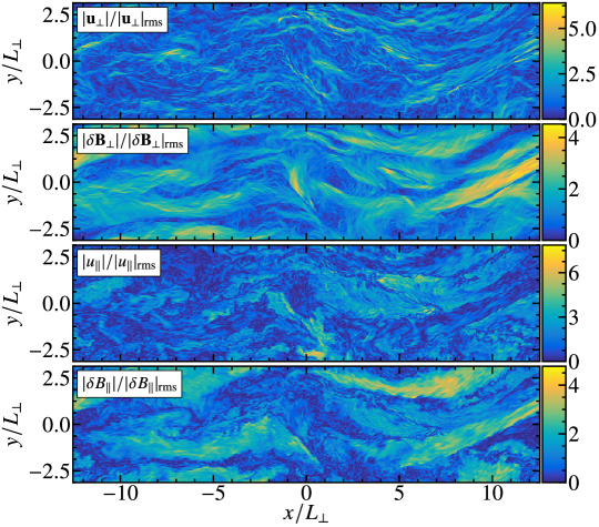
Figure 4: Snapshots of (from top to bottom) $|{\boldsymbol{\mathrm{u}}}_{\perp}|$, $|\delta{\boldsymbol{\mathrm{B}}}_{\perp}|$, $|u_{\|}|$, and $|\delta\!B_{\|}|$, each normalized by its own rms value. These snapshots are taken at $\Omega t=395$, $z=0$, and for $\beta=1$.

The difference of filamentation levels is more transparent in Fig. 5, which shows the energy spectra of all fields vs. $k_{\perp}$, compensated by $k_{\perp}^{3/2}$. Here, the energy spectrum of each integrand in (4a) and (4b) is denoted by $E$ with the corresponding subscript. We find that, for the compressive fields, both $E_{u_{\|}}$ and $E_{\delta\!B_{\|}}$ have $\simeq-3/2$ slope, while the slopes of the Alfvénic fields are not identifiable with the current numerical resolution. Independently of $\beta$, $E_{u_{\perp}}$ is subdominant compared to $E_{\delta\!B_{\perp}}$ at the injection scales, whereas $E_{u_{\|}}$ and $E_{\delta\!B_{\|}}$ have almost the same amplitudes throughout the whole $k_{\perp}$ range. It is well known that full-MHD simulations of MRI turbulence yield magnetically dominated spectra at large scales (e.g., Lesur & Longaretti, 2011; Walker et al., 2016; Kimura et al., 2016; Sun & Bai, 2021), due to generation of azimuthal magnetic field through the shear-flow effect. However, this mechanism cannot explain $E_{\delta\!B_{\perp}}\gg E_{u_{\perp}}$ in RRMHD because the shear flow does not directly produce $\delta{\boldsymbol{\mathrm{B}}}_{\perp}$, as one can see in (3a). Instead we can explain the dominance of $E_{\delta\!B_{\perp}}$ by the linear relation $\Psi/\Phi=k_{\|}v_{\mathrm{A}}/\gamma$ given by (3a), where $\gamma$ is the growth rate of MRI. For the fastest growing mode, $k_{\|}v_{\mathrm{A}}/\Omega\simeq 1$ and $\gamma/\Omega<1$ (see Fig. 2), meaning that the linear MRI in RRMHD excites $\delta\!B_{\perp}$ preferentially over $u_{\perp}$. One also finds from Fig. 5 that the disparity between $\delta\!B_{\perp}$ and $u_{\perp}$ gets smaller as $\beta$ increases. More specifically, at $k_{\perp}L_{\perp}=1$, $E_{\delta\!B_{\perp}}/E_{u_{\perp}}\simeq$ 27, 12, and 10 for $\beta=$ 0.1, 1, and 10, respectively, being consistent with the fact that $\gamma_{\mathrm{max}}/\Omega$ is an increasing function of $\beta$. Nonetheless, the absolute values of the ratio are somewhat different from the linear estimate $(\Psi/\Phi)^{2}\simeq$ 14, 3 and 2 for $\beta=$ 0.1, 1, and 10, respectively, for the fastest-growing mode. This indicates that the nonlinear effect is important, and, indeed, as we will see in Fig. 8, the partition of energy flux between Alfvénic and compressive fluctuations is different between the linear calculation and nonlinear simulations.

It is worthwhile to compare our spectra with the incompressible MRI simulation by Walker et al. (2016), which is the highest-resolution shearing box turbulence to date. They found that the slope of the magnetic field spectrum was close to -3/2 when the azimuthal component $B_{Y}$ was subtracted. They also found nearly -3/2 spectral slope for the velocity field as well. These spectra bear a resemblance to our spectra (Fig. 5). Note, however, that $B_{Y}$ is not necessarily the true mean magnetic field ${\boldsymbol{\mathrm{B}}}_{0}$, and thus, their magnetic spectrum $B_{X}^{2}+B_{Z}^{2}$ is presumably a mixture of parallel and perpendicular fluctuations.

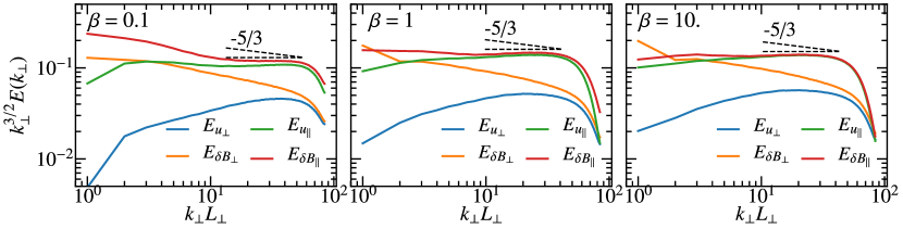
Figure 5: Magnetic and kinetic spectra compensated by $k_{\perp}^{3/2}$ and averaged over the time interval shown by the shaded area in Fig. 3 for high-resolution runs with (left) $\beta=0.1$, (middle) $\beta=1$, and (right) $\beta=10$. The dashed lines indicate the -3/2 and -5/3 slopes.

In order to investigate the decoupling of Alfvénic and compressive fluctuations, we compare the spectra of energy injection via MRI ($I_{\mathrm{MRI}}$), the energy exchange between the Alfvénic and compressive fluctuations ($I_{\mathrm{AW}}$), and the nonlinear energy transfer, defined below. Since the coupling between the Alfvénic and compressive fluctuations exists only through the linear terms, the two types of fluctuations are decoupled when the nonlinear energy transfer overwhelms $I_{\mathrm{AW}}$. The nonlinear energy transfer from all modes with wavenumber magnitudes smaller than $k_{\perp}$ are defined by (Alexakis et al., 2005; Grete et al., 2017; St-Onge et al., 2020)

$$\mathcal{N}_{\mathrm{AW}}^{<k_{\perp}} \equiv\sum_{|q_{\perp}|=k_{\perp}}\bigg{[}-{\boldsymbol{\mathrm{u}}}_{{\perp}{\boldsymbol{\mathrm{q}}}}^{*}\cdot\left({\boldsymbol{\mathrm{u}}}_{\perp}\cdot\nabla_{\perp}{\boldsymbol{\mathrm{u}}}_{\perp}^{[<k_{\perp}]}\right)_{\boldsymbol{\mathrm{q}}}+{\boldsymbol{\mathrm{u}}}_{{\perp}{\boldsymbol{\mathrm{q}}}}^{*}\cdot\left({\boldsymbol{\mathrm{b}}}_{\perp}\cdot\nabla_{\perp}{\boldsymbol{\mathrm{b}}}_{\perp}^{[<k_{\perp}]}\right)_{\boldsymbol{\mathrm{q}}}$$ (10)

$$\hskip 44.50003pt-{\boldsymbol{\mathrm{b}}}_{{\perp}{\boldsymbol{\mathrm{q}}}}^{*}\cdot\left({\boldsymbol{\mathrm{u}}}_{\perp}\cdot\nabla_{\perp}{\boldsymbol{\mathrm{b}}}_{\perp}^{[<k_{\perp}]}\right)_{\boldsymbol{\mathrm{q}}}+{\boldsymbol{\mathrm{b}}}_{{\perp}{\boldsymbol{\mathrm{q}}}}^{*}\cdot\left({\boldsymbol{\mathrm{b}}}_{\perp}\cdot\nabla_{\perp}{\boldsymbol{\mathrm{u}}}_{\perp}^{[<k_{\perp}]}\right)_{\boldsymbol{\mathrm{q}}}\bigg{]}$$ (11)

$$\mathcal{N}_{\mathrm{compr}}^{<k_{\perp}} \equiv\sum_{|q_{\perp}|=k_{\perp}}\bigg{[}-u_{\|{\boldsymbol{\mathrm{q}}}}^{*}\cdot\left({\boldsymbol{\mathrm{u}}}_{\perp}\cdot\nabla_{\perp}u_{\|}^{[<k_{\perp}]}\right)_{\boldsymbol{\mathrm{q}}}+u_{\|{\boldsymbol{\mathrm{q}}}}^{*}\cdot\left({\boldsymbol{\mathrm{b}}}_{\perp}\cdot\nabla_{\perp}b_{\|}^{[<k_{\perp}]}\right)_{\boldsymbol{\mathrm{q}}}$$ (12)

$$\hskip 44.50003pt-b_{\|{\boldsymbol{\mathrm{q}}}}^{*}\cdot\left({\boldsymbol{\mathrm{u}}}_{\perp}\cdot\nabla_{\perp}b_{\|}^{[<k_{\perp}]}\right)_{\boldsymbol{\mathrm{q}}}+b_{\|{\boldsymbol{\mathrm{q}}}}^{*}\cdot\left({\boldsymbol{\mathrm{b}}}_{\perp}\cdot\nabla_{\perp}u_{\|}^{[<k_{\perp}]}\right)_{\boldsymbol{\mathrm{q}}}\bigg{]},$$ (13)

where $f^{[<k_{\perp}]}({\boldsymbol{\mathrm{r}}})\equiv\sum_{q_{z}}\sum_{q_{\perp}<k_{\perp}}f_{\boldsymbol{\mathrm{q}}}\mathrm{e}^{\mathrm{i}{\boldsymbol{\mathrm{q}}}\cdot{\boldsymbol{\mathrm{r}}}}$, ${\boldsymbol{\mathrm{b}}}\equiv v_{\mathrm{A}}\delta{\boldsymbol{\mathrm{B}}}/B_{0}$. We also define the spectra of MRI injection $I_{\mathrm{MRI}}=\sum_{\boldsymbol{\mathrm{k}}}\mathcal{I}_{\mathrm{MRI}}({\boldsymbol{\mathrm{k}}})$ and energy exchange $I_{\mathrm{AW}}=\sum_{\boldsymbol{\mathrm{k}}}\mathcal{I}_{\mathrm{AW}}({\boldsymbol{\mathrm{k}}})$. The top panels of Fig. 6 show the perpendicular spectra of injection, exchange, and nonlinear energy transfer. Both the injection and exchange peak near the box scale and drop quickly at smaller scales, while the nonlinear energy transfer is relatively constant throughout the $k_{\perp}$-range. Consequently, the nonlinear energy transfer overwhelms the injection and coupling immediately below the box scale. The bottom panels of Fig. 6 show the $z$ spectra of the same quantities. The peak of the injection is located around $k_{z}v_{\mathrm{A}}/\Omega\simeq 1$, and thus, the injection scale corresponds to the fastest-growing modes. In the same way as the perpendicular spectra, the injection and exchange drop quickly at scales smaller than that of the fastest-growing mode and are overwhelmed by the nonlinear energy transfer. Therefore, in the small scales of our simulations, the coupling between Alfvénic and compressive fluctuations is negligible.

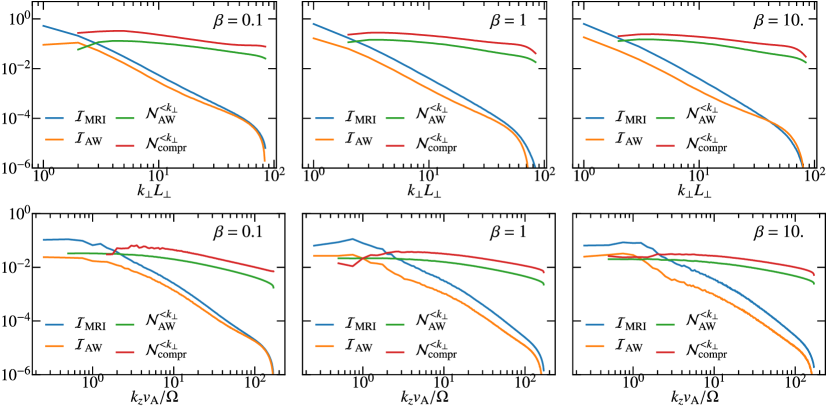
Figure 6: The spectra of energy injection via MRI, energy exchange between Alfvénic and compressive fluctuations, dissipation of Alfvénic and compressive fluctuations, and nonlinear transfer vs. (top) $k_{\perp}$ and (bottom) $k_{z}$ for (left) $\beta=0.1$, (middle) $\beta=1$, and (right) $\beta=10$. The spectra are normalized by $\langle I_{\mathrm{MRI}}\rangle$, integrated over (top) $k_{z}$ and (bottom) $k_{\perp}$, and averaged over the time interval shown by the shaded area in Fig. 3.

While the spectral comparison shown in Fig. 6 is the most direct proof of the decoupling of Alfvénic and compressive fluctuations, we expect that the ratio between the eddy-turnover rate and the angular velocity of the accretion disc can also be a proxy for the measurement of the decoupling. In Fig. 7, we plot the eddy-turnover rate $\omega_{\mathrm{nl}}\sim|{\boldsymbol{\mathrm{u}}}_{\perp}\cdot\nabla_{\perp}|\sim k_{\perp}u_{\perp}\sim k_{\perp}^{3/2}E_{u_{\perp}}^{1/2}$ normalized by $\Omega$. One finds that this value is an increasing function of $k_{\perp}L_{\perp}$ and exceeds unity at some scale. As mentioned above, when $\omega_{\mathrm{nl}}/\Omega$ is much larger than unity, the effect of differential rotation is expected to be negligible, and the turbulence obeys the standard RMHD where the Alfvénic and compressive fluctuations are decoupled (Schekochihin et al., 2009). The scale at which $\omega_{\mathrm{nl}}/\Omega\simeq 1$ is not much smaller than the injection scale, which is consistent with the fact that the nonlinear energy transfer overwhelms the MRI injection immediately below the injection scale, as shown in Fig. 6. In general, $\omega_{\mathrm{nl}}/\Omega$ is easier to use as an indicator of decoupling because computing the nonlinear energy transfer is numerically cumbersome.

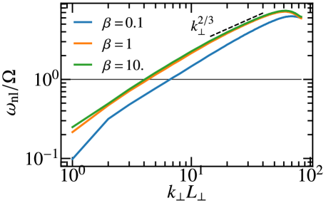
Figure 7: Normalized eddy turnover frequency $\omega_{\mathrm{nl}}/(\Omega\cos\theta)$ vs. $k_{\perp}L_{\perp}$ averaged over the time interval shown by the shaded area in Fig. 3 for higher-resolution runs. The effect of differential rotation is negligible where the value is greater than unity.

As the decoupling of Alfvénic and compressive fluctuations in our simulations has been demonstrated in Figs. 6 and 7, we now calculate the partition of energy flux carried by these two types of fluctuations. Figure 8 shows the dependence of $\langle D_{\mathrm{compr}}\rangle/\langle D_{\mathrm{AW}}\rangle$ on $\beta$. We find that $\langle D_{\mathrm{compr}}\rangle/\langle D_{\mathrm{AW}}\rangle$ is between 2 and 2.5 for all values of $\beta$ that we studied, without an obvious trend. Since Alfvénic and compressive fluctuations are decoupled, the result in Fig 8 would not be changed for a finer-resolution simulation. Indeed, we have found almost identical values of $\langle D_{\mathrm{compr}}\rangle/\langle D_{\mathrm{AW}}\rangle$ in our simulations conducted at all resolutions, from low to high. This is because, as seen in Fig. 6, even the low-resolution-grid runs resolve the critical scale where the nonlinear energy transfer dominates the linear coupling.

Note that the values of $\langle D_{\mathrm{compr}}\rangle/\langle D_{\mathrm{AW}}\rangle$ obtained from our nonlinear simulations are different from the values of $I_{\mathrm{compr}}/I_{\mathrm{AW}}$ [see (27) for the definition] computed “quasilinearly” for the fastest-growing linear MRI modes (black dashed line in Fig 8), the latter value being close to unity. This indicates that, even though the decoupling of Alfvénic and compressive fluctuations starts relatively near the injection scale, the preferential excitation of compressive fluctuations in MRI turbulence is the consequence of nonlinear effects, i.e., of the way in which the nonlinearity removes the energy injected by the MRI from the injection scale and transfers it into the two turbulent cascade.

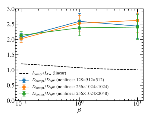
Figure 8: Partition of energy flux between Alfvénic and compressive fluctuations vs. $\beta$: (black) $I_{\mathrm{compr}}/I_{\mathrm{AW}}$ calculated by the eigenfunctions of linear dispersion relation (7) and $D_{\mathrm{compr}}/D_{\mathrm{AW}}$ calculated by the nonlinear simulation with (blue) low-resolution grids, (orange) medium-resolution grids, (green) high-resolution grids. Error bars for the nonlinear simulations are estimated by calculating the standard deviation over the averaging interval.

5 Application to ion-to-electron heating prescription in hot accretion flows

In this section, we discuss the application of our findings to hot accretion flows, such as M87 and Sgr A*, together with some important caveats. Numerical simulations of gyrokinetic turbulence have revealed that the partition between ion and electron heating is crucially sensitive to the compressive-to-Alfvénic injection power ratio $P_{\mathrm{compr}}/P_{\mathrm{AW}}$ at the ion Larmor scale (Kawazura et al., 2020). Since the compressive and Alfvénic energy fluxes computed in our simulations are supposed to cascade down to the ion Larmor scale independently, it is straightforward to infer that $P_{\mathrm{compr}}/P_{\mathrm{AW}}$ is equal to $D_{\mathrm{compr}}/D_{\mathrm{AW}}\simeq 2-2.5$, as we found in Fig. 8. Therefore, we can combine the results of this paper with our previous stydy of gyrokinetic turbulence to formulate the ion-to-electron heating prescription that incorporates both driving of turbulence via MRI at MHD scales and the dissipation at kinetic scales. Substituting $P_{\mathrm{compr}}/P_{\mathrm{AW}}=2$ in (14) of  Kawazura et al. (2019), one obtains

$$\frac{Q_{\mathrm{i}}}{Q_{\mathrm{e}}}(\beta_{\mathrm{i}},\,T_{\mathrm{i}}/T_{\mathrm{e}})=\frac{35}{1+(\beta_{\mathrm{i}}/15)^{-1.4}\mathrm{e}^{-0.1/(T_{\mathrm{i}}/T_{\mathrm{e}})}}+2,$$ (14)

where $T_{\mathrm{i}}/T_{\mathrm{e}}$ is the ion-to-electron background temperature ratio, and $\beta_{\mathrm{i}}$ is the ion beta.

This prescription is a step forward from the currently used heating prescription and may help improve the quality of hot accretion flow modelling (e.g., Chael et al., 2018, 2019). However, one must bear in mind that a number of heating channels are missing in (14). First, we do not consider spiral density waves (Heinemann & Papaloizou, 2009) which are outside the RMHD ordering as they have no vertical structure, i.e., $k_{Z}\simeq 0$. The excitation of these waves may change the partition between Alfvénic and compressive fluctuations. Note that these waves form weak shocks and dissipate into thermal energy, but the amount of heating due to this dissipation is very little.

Second, while we have only considered collisional MRI in this study, the mean free path of hot accretion flows is almost equal to, or longer than, the scale height of the disc, meaning that MRI is supposed to be collisionless. When MRI is collisionless, the viscous stress due to pressure anisotropy gives rise to a new heating channel. About 50% of total injected power may be directly converted into heat at large scales by this viscous stress, which would not cascade down to the ion Larmor scale (Sharma et al., 2007; Kempski et al., 2019).

Third, even if these additional heating channels at large scales are absent, there are other heating channels at the ion Larmor scale that are not captured by standard gyrokinetics (see Sec. II A in Kawazura et al., 2020, for a detailed discussion), e.g., cyclotron heating (Cranmer et al., 1999), stochastic heating (Chandran et al., 2010), and background pressure anisotropy (Kunz et al., 2018).

Thus, our heating prescription (14) is only the simplest possible model that considers both MRI injection and kinetic dissipation. Including the missing heating channels is an important task for future work.

6 Conclusions

In this study, we have calculated the energy partition between Alfvénic and compressive fluctuations in turbulence driven by MRI with near-azimuthal mean magnetic fields. The fastest-growing MRI modes are correctly captured by RMHD with differential rotation (RRMHD) because they satisfy $|k_{Z}/k_{Y}|\sim|k_{\perp}/k_{\|}|\gg 1$ when the background field is nearly azimuthal (Balbus & Hawley, 1992a). In RRMHD, the Alfvénic and compressive fluctuations are coupled only through the linear terms that are proportional to the angular velocity of the accretion disc. We have carried out nonlinear simulations of RRMHD and showed that the nonlinear energy transfer overwhelms the linear coupling immediately below the injection scale. Thus, the two kinds of fluctuations are decoupled at the small scales in our simulations. This is because, below the injection scale, the eddy turnover time is much shorter than the disc rotation time, i.e., $\omega_{\mathrm{nl}}/\Omega\gg 1$. Most importantly, the energy flux carried by the compressive fluctuations is more than double that carried by the Alfvénic fluctuations at the decoupled scales — a result reflecting the interaction between MRI injection and nonlinearity at the injection scale and distinct from a “quasilinear” estimate (which suggests near equipartition).

While these findings suggest that RRMHD is a useful model for studying MRI turbulence, we would like to stress the following two limitations of the RMHD approach for MRI-driven turbulence in accretion flows. First, we assume a near-azimuthal constant mean magnetic field. This may be quite restrictive: e.g., global MHD simulations (e.g., Suzuki & Inutsuka, 2014) sometimes exhibit non-azimuthal components of magnetic field. Secondly, we assume that $k_{\|}/k_{\perp}\ll 1$ is already satisfied at a larger scale than the critical scale where $\omega_{\mathrm{nl}}/\Omega\sim 1$. If this were not to hold, the rotation effects in full-MHD may become negligible at scales larger than those where the RMHD approximation is already satisfied, and our RRMHD model would not be a good model of MRI turbulence at the decoupling scale. In such a case, the turbulence in the RMHD range would not be driven by MRI, but by the cascade from the full-MHD scales. A simulation of full-MHD with extreme resolutions is necessary to explore this possibility.

Declaration of interests

The authors report no conflict of interest.

Appendix A Derivation of RRMHD model

Here, we explicitly derive (3a)-(3d) from (1a)-(1d). The way we do it is mostly the same as the derivation of (17), (18), (25), and (26) in Schekochihin et al. (2009), but with account taken of the differential rotation of the disc. We start by considering the following ordering:

$$\frac{{\boldsymbol{\mathrm{u}}}}{v_{\mathrm{A}}}\sim\frac{\delta{\boldsymbol{\mathrm{B}}}}{B_{0}}\sim\frac{k_{\|}}{k_{\perp}}\sim\sin\theta\sim\epsilon,\quad\frac{\p}{\p t}\sim\Omega\sim k_{\|}v_{\mathrm{A}}\equiv\omega.$$ (15)

Then, the order of each term in (1a) is estimated as follows:

$$\underbrace{\frac{\p}{\p t}\frac{\delta\!\rho}{\rho_{0}}}_{\epsilon^{1}\omega}+\underbrace{u_{\|}\frac{\p}{\p z}\frac{\delta\!\rho}{\rho_{0}}}_{\epsilon^{2}\omega}+\underbrace{{\boldsymbol{\mathrm{u}}}_{\perp}\cdot\nabla_{\perp}\frac{\delta\!\rho}{\rho_{0}}}_{\epsilon^{1}\omega}-\underbrace{q\Omega x\sin\theta\Bigg{(}\frac{\p}{\p y}+\frac{1}{\tan\theta}\frac{\p}{\p z}\Bigg{)}}_{\epsilon^{2}\omega}\frac{\delta\!\rho}{\rho_{0}}\\ =-\Bigg{(}\underbrace{\frac{\p u_{\|}}{\p z}}_{\epsilon^{1}\omega}+\underbrace{\nabla_{\perp}\cdot{\boldsymbol{\mathrm{u}}}_{\perp}}_{\epsilon^{0}\omega}\Bigg{)}-\frac{\delta\!\rho}{\rho_{0}}\Bigg{(}\underbrace{\frac{\p u_{\|}}{\p z}}_{\epsilon^{2}\omega}+\underbrace{\nabla_{\perp}\cdot{\boldsymbol{\mathrm{u}}}_{\perp}}_{\epsilon^{1}\omega}\Bigg{)}.$$ (16)

To order $\mathcal{O}(\epsilon^{0}\omega)$, we obtain $\nabla_{\perp}\cdot{\boldsymbol{\mathrm{u}}}_{\perp}=0$. Likewise, to lowest-order, $\nabla\cdot\delta{\boldsymbol{\mathrm{B}}}=0$ gives $\nabla_{\perp}\cdot\delta{\boldsymbol{\mathrm{B}}}_{\perp}=0$. Therefore, we may write ${\boldsymbol{\mathrm{u}}}_{\perp}$ and $\delta{\boldsymbol{\mathrm{B}}}_{\perp}$ in terms of stream and flux functions:

$${\boldsymbol{\mathrm{u}}}_{\perp}=\hat{{\boldsymbol{\mathrm{z}}}}\times\nabla_{\perp}\Phi,\quad\frac{\delta{\boldsymbol{\mathrm{B}}}_{\perp}}{B_{0}}=\frac{\hat{{\boldsymbol{\mathrm{z}}}}\times\nabla_{\perp}\Psi}{v_{\mathrm{A}}}.$$ (17)

Then, the $\mathcal{O}(\epsilon^{1}\omega)$ terms in (16) yield

$$\left(\frac{\p}{\p t}+{\boldsymbol{\mathrm{u}}}_{\perp}\cdot\nabla_{\perp}\right)\frac{\delta\!\rho}{\rho_{0}}=-\frac{\p u_{\|}}{\p z}.$$ (18)

Note that the shearing term, viz., the fourth term in the left-hand side of (16), is ordered out. As we will show shortly, the shearing terms in other equations are also ordered out.

Under the same ordering, terms in (1b) are ordered as follows:

$$\underbrace{\frac{\p{\boldsymbol{\mathrm{u}}}}{\p t}}_{\epsilon^{1}\omega v_{\mathrm{A}}}+\underbrace{u_{\|}\frac{\p{\boldsymbol{\mathrm{u}}}}{\p z}}_{\epsilon^{2}\omega v_{\mathrm{A}}}+\underbrace{{\boldsymbol{\mathrm{u}}}_{\perp}\cdot\nabla_{\perp}{\boldsymbol{\mathrm{u}}}}_{\epsilon^{1}\omega v_{\mathrm{A}}}-\underbrace{q\Omega x\sin\theta\Bigg{(}\frac{\p}{\p y}+\frac{1}{\tan\theta}\frac{\p}{\p z}\Bigg{)}}_{\epsilon^{2}\omega v_{\mathrm{A}}}{\boldsymbol{\mathrm{u}}}=-\hat{{\boldsymbol{\mathrm{z}}}}\frac{\p}{\p z}\Bigg{[}\underbrace{\frac{c_{\mathrm{S}}^{2}}{\Gamma}\frac{\delta\!p}{p_{0}}}_{\epsilon^{1}\omega v_{\mathrm{A}}}+v_{\mathrm{A}}^{2}\Bigg{(}\underbrace{\frac{1}{2}\frac{|\delta{\boldsymbol{\mathrm{B}}}|^{2}}{B_{0}^{2}}}_{\epsilon^{2}\omega v_{\mathrm{A}}}+\underbrace{\frac{\delta\!B_{\|}}{B_{0}}}_{\epsilon^{1}\omega v_{\mathrm{A}}}\Bigg{)}\Bigg{]}\\ -\nabla_{\perp}\Bigg{[}\underbrace{\frac{c_{\mathrm{S}}^{2}}{\Gamma}\frac{\delta\!p}{p_{0}}}_{\epsilon^{0}\omega v_{\mathrm{A}}}+v_{\mathrm{A}}^{2}\Bigg{(}\underbrace{\frac{1}{2}\frac{|\delta{\boldsymbol{\mathrm{B}}}|^{2}}{B_{0}^{2}}}_{\epsilon^{1}\omega v_{\mathrm{A}}}+\underbrace{\frac{\delta\!B_{\|}}{B_{0}}}_{\epsilon^{0}\omega v_{\mathrm{A}}}\Bigg{)}\Bigg{]}-\frac{\delta\rho}{\rho_{0}}\hat{{\boldsymbol{\mathrm{z}}}}\frac{\p}{\p z}\Bigg{[}\underbrace{\frac{c_{\mathrm{S}}^{2}}{\Gamma}\frac{\delta\!p}{p_{0}}}_{\epsilon^{2}\omega v_{\mathrm{A}}}+v_{\mathrm{A}}^{2}\Bigg{(}\underbrace{\frac{1}{2}\frac{|\delta{\boldsymbol{\mathrm{B}}}|^{2}}{B_{0}^{2}}}_{\epsilon^{3}\omega v_{\mathrm{A}}}+\underbrace{\frac{\delta\!B_{\|}}{B_{0}}}_{\epsilon^{2}\omega v_{\mathrm{A}}}\Bigg{)}\Bigg{]}\\ -\frac{\delta\rho}{\rho_{0}}\nabla_{\perp}\Bigg{[}\underbrace{\frac{c_{\mathrm{S}}^{2}}{\Gamma}\frac{\delta\!p}{p_{0}}}_{\epsilon^{1}\omega v_{\mathrm{A}}}+v_{\mathrm{A}}^{2}\Bigg{(}\underbrace{\frac{1}{2}\frac{|\delta{\boldsymbol{\mathrm{B}}}|^{2}}{B_{0}^{2}}}_{\epsilon^{2}\omega v_{\mathrm{A}}}+\underbrace{\frac{\delta\!B_{\|}}{B_{0}}}_{\epsilon^{1}\omega v_{\mathrm{A}}}\Bigg{)}\Bigg{]}+v_{\mathrm{A}}^{2}\Bigg{(}\underbrace{\frac{\p}{\p z}\frac{\delta{\boldsymbol{\mathrm{B}}}}{B_{0}}}_{\epsilon^{1}\omega v_{\mathrm{A}}}+\underbrace{\frac{\delta\!B_{\|}}{B_{0}}\frac{\p}{\p z}\frac{\delta{\boldsymbol{\mathrm{B}}}}{B_{0}}}_{\epsilon^{2}\omega v_{\mathrm{A}}}+\underbrace{\frac{\delta{\boldsymbol{\mathrm{B}}}_{\perp}}{B_{0}}\cdot\nabla_{\perp}\frac{\delta{\boldsymbol{\mathrm{B}}}}{B_{0}}}_{\epsilon^{1}\omega v_{\mathrm{A}}}\Bigg{)}\\ -2\Omega(-\underbrace{\cos\theta\,\hat{{\boldsymbol{\mathrm{y}}}}}_{\epsilon^{2}\omega v_{\mathrm{A}}}+\underbrace{\sin\theta\,\hat{{\boldsymbol{\mathrm{z}}}}}_{\epsilon^{1}\omega v_{\mathrm{A}}})\times{\boldsymbol{\mathrm{u}}}+q\Omega u_{x}(\underbrace{\sin\theta\,\hat{{\boldsymbol{\mathrm{y}}}}}_{\epsilon^{2}\omega v_{\mathrm{A}}}+\underbrace{\cos\theta\,\hat{{\boldsymbol{\mathrm{z}}}}}_{\epsilon^{1}\omega v_{\mathrm{A}}}).$$ (19)

From the $\mathcal{O}(\epsilon^{0}\omega v_{\mathrm{A}})$ terms in (19), one gets the pressure balance

$$\frac{c_{\mathrm{S}}^{2}}{\Gamma}\frac{\delta\!p}{p_{0}}+v_{\mathrm{A}}^{2}\frac{\delta\!B_{\|}}{B_{0}}=0,$$ (20)

which, when combined with (1d), becomes

$$\frac{\delta\!\rho}{\rho_{0}}+\frac{v_{\mathrm{A}}^{2}}{c_{\mathrm{S}}^{2}}\frac{\delta\!B_{\|}}{B_{0}}=0.$$ (21)

From the $\mathcal{O}(\epsilon^{1}\omega v_{\mathrm{A}})$ terms in (19), we obtain

$$\frac{\p{\boldsymbol{\mathrm{u}}}}{\p t}+{\boldsymbol{\mathrm{u}}}_{\perp}\cdot\nabla_{\perp}{\boldsymbol{\mathrm{u}}}=-\nabla_{\perp}\Bigg{(}\frac{v_{\mathrm{A}}^{2}}{2}\frac{|\delta{\boldsymbol{\mathrm{B}}}|^{2}}{B_{0}^{2}}\Bigg{)}+v_{\mathrm{A}}^{2}\Bigg{(}\frac{\p}{\p z}\frac{\delta{\boldsymbol{\mathrm{B}}}}{B_{0}}+\frac{\delta{\boldsymbol{\mathrm{B}}}_{\perp}}{B_{0}}\cdot\nabla_{\perp}\frac{\delta{\boldsymbol{\mathrm{B}}}}{B_{0}}\Bigg{)}\\ +2\Omega\hat{{\boldsymbol{\mathrm{y}}}}\times{\boldsymbol{\mathrm{u}}}+q\Omega u_{x}\hat{{\boldsymbol{\mathrm{z}}}},$$ (22)

where we have used $\cos\theta\simeq 1$ and neglected all terms containing $\sin\theta\ll 1$. The desired perpendicular and parallel momentum equations (3b) and (3c) are recovered as $\hat{{\boldsymbol{\mathrm{z}}}}\cdot[\nabla_{\perp}\times$(22)] and $\hat{{\boldsymbol{\mathrm{z}}}}\cdot$(22), respectively.

Next, the ordering of terms in (1c) is as follows:

$$\underbrace{\frac{\p}{\p t}\frac{\delta{\boldsymbol{\mathrm{B}}}}{B_{0}}}_{\epsilon^{1}\omega}+\underbrace{u_{\|}\frac{\p}{\p z}\frac{\delta{\boldsymbol{\mathrm{B}}}}{B_{0}}}_{\epsilon^{2}\omega}+\underbrace{{\boldsymbol{\mathrm{u}}}_{\perp}\cdot\nabla_{\perp}\frac{\delta{\boldsymbol{\mathrm{B}}}}{B_{0}}}_{\epsilon^{1}\omega}-\underbrace{q\Omega x\sin\theta\Bigg{(}\frac{\p}{\p y}+\frac{1}{\tan\theta}\frac{\p}{\p z}\Bigg{)}}_{\epsilon^{2}\omega}\frac{\delta{\boldsymbol{\mathrm{B}}}}{B_{0}}+\Bigg{(}\underbrace{\hat{{\boldsymbol{\mathrm{z}}}}}_{\epsilon^{1}\omega}+\underbrace{\frac{\delta{\boldsymbol{\mathrm{B}}}}{B_{0}}}_{\epsilon^{2}\omega}\Bigg{)}\frac{\p u_{\|}}{\p z}\\ =\underbrace{\frac{\p{\boldsymbol{\mathrm{u}}}}{\p z}}_{\epsilon^{1}\omega}+\underbrace{\frac{\delta\!B_{\|}}{B_{0}}\frac{\p{\boldsymbol{\mathrm{u}}}}{\p z}}_{\epsilon^{2}\omega}+\underbrace{\frac{\delta{\boldsymbol{\mathrm{B}}}_{\perp}}{B_{0}}\cdot\nabla_{\perp}{\boldsymbol{\mathrm{u}}}}_{\epsilon^{1}\omega}-q\Omega\frac{\delta\!B_{x}}{B_{0}}(\underbrace{\sin\theta\hat{{\boldsymbol{\mathrm{y}}}}}_{\epsilon^{2}\omega}+\underbrace{\cos\theta\hat{{\boldsymbol{\mathrm{z}}}}}_{\epsilon^{1}\omega}).$$ (23)

Together with (18) and (21), the $\mathcal{O}(\epsilon^{1}\omega)$ terms in this equation yield

$$\left(\frac{\p}{\p t}+{\boldsymbol{\mathrm{u}}}_{\perp}\cdot\nabla_{\perp}\right)\left(\frac{\delta{\boldsymbol{\mathrm{B}}}}{B_{0}}+\hat{{\boldsymbol{\mathrm{z}}}}\frac{v_{\mathrm{A}}^{2}}{c_{\mathrm{S}}^{2}}\frac{\delta\!B_{\|}}{B_{0}}\right)=\left(\frac{\p}{\p z}+\frac{\delta{\boldsymbol{\mathrm{B}}}}{B_{0}}\cdot\nabla_{\perp}\right){\boldsymbol{\mathrm{u}}}-q\Omega\frac{\delta\!B_{x}}{B_{0}}\hat{{\boldsymbol{\mathrm{z}}}}.$$ (24)

Finally, we obtain the perpendicular and parallel magnetic field equations (3a) and (3d) as $\hat{{\boldsymbol{\mathrm{z}}}}\cdot[\mathrm{curl}^{-1}$(24)] and $\hat{{\boldsymbol{\mathrm{z}}}}\cdot$(24), respectively.

Appendix B Compressive-to-Alfvénic energy-injection ratio for a single linear MRI mode in RRMHD

Substituting the solution to the dispersion relation (7) back into the linearized RRMHD equations (3a)-(3d), one gets the linear relations

$$\frac{\delta\!B_{\|}}{B_{0}}=\lambda\frac{k_{y}\Psi}{v_{\mathrm{A}}},$$ (25a)

$$\Phi=-\frac{\omega}{k_{\|}v_{\mathrm{A}}}\Psi,$$ (25b)

$$u_{\|}=-\frac{\Omega}{k_{\|}v_{\mathrm{A}}}\left[\left(1+\frac{v_{\mathrm{A}}^{2}}{c_{\mathrm{S}}^{2}}\right)\lambda\frac{\omega}{\Omega}+q\right]k_{y}\Psi,$$ (25c)

where,

$$\lambda=\frac{5\mathrm{i}\beta}{2\sqrt{2}(k_{y}/k_{\perp})^{2}(6+5\beta)^{3/2}}\Big{[}-6\bar{k}_{\|}^{2}+7(k_{y}/k_{\perp})^{2}(6+5\beta)\\ -\sqrt{36\bar{k}_{\|}^{4}+(k_{y}/k_{\perp})^{2}(6+5\beta)^{2}+4(k_{y}/k_{\perp})^{2}\bar{k}_{\|}^{2}(6+5\beta)(3+20\beta)}\Big{]}\Big{[}\bar{k}_{\|}^{2}(6+10\beta)+(k_{y}/k_{\perp})^{2}(6+5\beta)\\ -\sqrt{36\bar{k}_{\|}^{4}+(k_{y}/k_{\perp})^{2}(6+5\beta)^{2}+4(k_{y}/k_{\perp})^{2}\bar{k}_{\|}^{2}(6+5\beta)(3+20\beta)}\Big{]}^{-1},$$ (26)

with $\bar{k}_{\|}=k_{\|}v_{\mathrm{A}}/\Omega$. For the fastest-growing mode, $\lambda$ reduces to $\sqrt{-5\beta/(5\beta+6)}$. Substituting (25a)-(25c) into (5a) and (5b), one obtains

$$\frac{I_{\mathrm{compr}}}{I_{\mathrm{AW}}}=-\frac{q\lambda(k_{\|}v_{\mathrm{A}})^{2}/[(1+v_{\mathrm{A}}^{2}/c_{\mathrm{S}}^{2})\lambda\Omega/\omega+q]+(2-q)\Omega\omega^{*}}{2\Omega\omega^{*}},$$ (27)

where the superscript star denotes the complex conjugate. Note that, when the rotation is not sheared, i.e., $q=0$, this becomes the conservation of energy $I_{\mathrm{compr}}+I_{\mathrm{AW}}=0$, i.e., the Alfvénic and compressive fluctuations exchange their energy via unsheared rotation.

References

- Alexakis et al. (2005) Alexakis, A., Mininni, P. D. & Pouquet, A. 2005 Shell-to-shell energy transfer in magnetohydrodynamics. I. Steady state turbulence. Phys. Rev. E 72, 046301.
- Balbus & Hawley (1991) Balbus, S. A. & Hawley, J. F. 1991 A powerful local shear instability in weakly magnetized disks. I - Linear analysis. II - Nonlinear evolution. Astrophys. J. 376, 214.
- Balbus & Hawley (1992a) Balbus, S. A. & Hawley, J. F. 1992a A powerful local shear instability in weakly magnetized disks. IV. Nonaxisymmetric perturbations. Astrophys. J. 400, 610.
- Balbus & Hawley (1992b) Balbus, S. A. & Hawley, J. F. 1992b Is the Oort A-value a universal growth rate limit for accretion disk shear instabilities? Astrophys. J. 392, 662.
- Balbus & Hawley (1998) Balbus, S. A. & Hawley, J. F. 1998 Instability, turbulence, and enhanced transport in accretion disks. Rev. Mod. Phys. 70, 1.
- Chael et al. (2019) Chael, A., Narayan, R. & Johnson, M. D. 2019 Two-temperature, magnetically arrested disc simulations of the jet from the supermassive black hole in M87. Mon. Not. R. Astron. Soc. 486, 2873.
- Chael et al. (2018) Chael, A., Rowan, M., Narayan, R., Johnson, M. & Sironi, L. 2018 The role of electron heating physics in images and variability of the Galactic Centre black hole Sagittarius A*. Mon. Not. R. Astron. Soc. 478, 5209.
- Chandra et al. (2017) Chandra, M., Foucart, F. & Gammie, C. F. 2017 grim: A Flexible, Conservative Scheme for Relativistic Fluid Theories. Astrophys. J. 837 (1), 92.
- Chandra et al. (2015) Chandra, M., Gammie, C. F., Foucart, F. & Quataert, E. 2015 An Extended Magnetohydrodynamics Model for Relativistic Weakly Collisional Plasmas. Astrophys. J. 810 (2), 162.
- Chandran et al. (2010) Chandran, B. D. G., Li, B., Rogers, B. N., Quataert, E. & Germaschewski, K. 2010 Perpendicular ion heating by low-frequency Alfvén-wave turbulence in the solar Wind. Astrophys. J. 720 (1), 503–515.
- Cho & Lazarian (2002) Cho, J. & Lazarian, A. 2002 Compressible sub-Alfvénic MHD turbulence in low- plasmas. Phys. Rev. Lett. 88, 245001.
- Cho & Lazarian (2003) Cho, J. & Lazarian, A. 2003 Compressible magnetohydrodynamic turbulence: mode coupling, scaling relations, anisotropy, viscosity-damped regime and astrophysical implications. Mon. Not. R. Astron. Soc. 345, 325.
- Cranmer et al. (1999) Cranmer, S. R., Field, G. B. & Kohl, J. L. 1999 Spectroscopic constraints on models of ion cyclotron resonance heating in the polar solar corona and high-speed solar wind. Astrophys. J. 518 (2), 937–947.
- EHT Collaboration (2019) EHT Collaboration 2019 First M87 Event Horizon Telescope results. I. The shadow of the supermassive black hole. Astrophys. J. Lett. 875, L1.
- Foucart et al. (2016) Foucart, F., Chandra, M., Gammie, C. F. & Quataert, E. 2016 Evolution of accretion discs around a kerr black hole using extended magnetohydrodynamics. Mon. Not. R. Astron. Soc. 456 (2), 1332–1345.
- Foucart et al. (2017) Foucart, F., Chandra, M., Gammie, C. F., Quataert, E. & Tchekhovskoy, A. 2017 How important is non-ideal physics in simulations of sub-Eddington accretion on to spinning black holes? Mon. Not. R. Astron. Soc. 470 (2), 2240–2252.
- Goldreich & Lynden-Bell (1965) Goldreich, P. & Lynden-Bell, D. 1965 II. Spiral arms as sheared gravitational instabilities. Mon. Not. R. Astron. Soc. 130, 125.
- Goldreich & Sridhar (1995) Goldreich, P. & Sridhar, S. 1995 Toward a theory of interstellar turbulence. 2: Strong Alfvénic turbulence. Astrophys. J. 438, 763.
- Goldreich & Sridhar (1997) Goldreich, P. & Sridhar, S. 1997 Magnetohydrodynamic Turbulence Revisited. Astrophys. J. 485, 680.
- Grete et al. (2017) Grete, P., O’Shea, B. W., Beckwith, K., Schmidt, W. & Christlieb, A. 2017 Energy transfer in compressible magnetohydrodynamic turbulence. Phys. Plasmas 24, 092311.
- Hawley & Balbus (1992) Hawley, J. F. & Balbus, S. A. 1992 A powerful local shear instability in weakly magnetized disks. III. Long-term evolution in a shearing Sheet. Astrophys. J. 400, 595.
- Heinemann & Papaloizou (2009) Heinemann, T. & Papaloizou, J. C. B. 2009 The excitation of spiral density waves through turbulent fluctuations in accretion discs - II. Numerical simulations with MRI-driven turbulence. Mon. Not. R. Astron. Soc. 397 (1), 64–74.
- Hirai et al. (2018) Hirai, K., Katoh, Y., Terada, N. & Kawai, S. 2018 Study of the transition from MRI to magnetic turbulence via parasitic instability by a high-order MHD simulation code. Astrophys. J. 853, 174.
- Julien & Knobloch (2006) Julien, K. & Knobloch, E. 2006 Saturation of the magnetorotational instability: Asymptotically exact theory. In EAS Publications Series (ed. Michel Rieutord & Berengere Dubrulle), EAS Publications Series, vol. 21, p. 81.
- Kadomtsev & Pogutse (1974) Kadomtsev, B. B. & Pogutse, O. P. 1974 Nonlinear helical perturbations of a plasma in the tokamak. Sov. Phys.–JETP 38, 283.
- Kawazura (2022) Kawazura, Y. 2022 Calliope: Pseudospectral shearing magnetohydrodynamics code with a pencil decomposition. arXiv:2201.10416 .
- Kawazura et al. (2019) Kawazura, Y., Barnes, M. & Schekochihin, A. A. 2019 Thermal disequilibration of ions and electrons by collisionless plasma turbulence. Proc. Nat. Acad. Sci. 116, 771.
- Kawazura et al. (2020) Kawazura, Y., Schekochihin, A. A., Barnes, M., TenBarge, J. M., Tong, Y., Klein, K. G. & Dorland, W. 2020 Ion versus electron heating in compressively driven astrophysical gyrokinetic turbulence. Phys. Rev. X 10, 041050.
- Kempski et al. (2019) Kempski, P., Quataert, E., Squire, J. & Kunz, M. W. 2019 Shearing-box simulations of MRI-driven turbulence in weakly collisional accretion discs. Mon. Not. R. Astron. Soc. 486, 4013.
- Kim & Ostriker (2000) Kim, W.-T. & Ostriker, E. C. 2000 Magnetohydrodynamic Instabilities in Shearing, Rotating, Stratified Winds and Disks. Astrophys. J. 540 (1), 372–403.
- Kimura et al. (2016) Kimura, S. S., Toma, K., Suzuki, T. K. & Inutsuka, S.-i. 2016 Stochastic Particle Acceleration in Turbulence Generated by Magnetorotational Instability. Astrophys. J. 822, 88.
- Kraichnan (1965) Kraichnan, R. H. 1965 Inertial-Range spectrum of hydromagnetic turbulence. Phys. Fluids 8, 1385.
- Kunz et al. (2018) Kunz, M. W., Abel, I. G., Klein, K. G. & Schekochihin, A. A. 2018 Astrophysical gyrokinetics: turbulence in pressure-anisotropic plasmas at ion scales and beyond. Journal of Plasma Physics 84 (2), 715840201.
- Kunz et al. (2016) Kunz, M. W., Stone, J. M. & Quataert, E. 2016 Magnetorotational Turbulence and Dynamo in a Collisionless Plasma. Phys. Rev. Lett. 117 (23), 235101.
- Lesur & Longaretti (2011) Lesur, G. & Longaretti, P. Y. 2011 Non-linear energy transfers in accretion discs MRI turbulence. I. Net vertical field case. Astron. Astrophys. 528, A17.
- Lesur (2021) Lesur, G. R. J. 2021 Magnetohydrodynamics of protoplanetary discs. J. Plasma Phys. 87, 205870101.
- Makwana & Yan (2020) Makwana, K. D. & Yan, H. 2020 Properties of magnetohydrodynamic modes in compressively driven plasma turbulence. Phys. Rev. X 10, 031021.
- Mamatsashvili et al. (2013) Mamatsashvili, G. R., Chagelishvili, G. D., Bodo, G. & Rossi, P. 2013 Revisiting linear dynamics of non-axisymmetric perturbations in weakly magnetized accretion discs. Mon. Not. R. Astron. Soc. 435, 2552.
- Morrison et al. (2013) Morrison, P. J., Tassi, E. & Tronko, N. 2013 Stability of compressible reduced magnetohydrodynamic equilibria–Analogy with magnetorotational instability. Phys. Plasmas 20, 042109.
- Nazarenko & Schekochihin (2011) Nazarenko, S. V. & Schekochihin, A. A. 2011 Critical balance in magnetohydrodynamic, rotating and stratified turbulence: towards a universal scaling conjecture. J. Fluid Mech. 677, 134.
- Quataert et al. (2002) Quataert, E., Dorland, W. & Hammett, G. W. 2002 The Magnetorotational Instability in a Collisionless Plasma. Astrophys. J. 577, 524.
- Schekochihin (2020) Schekochihin, A. A. 2020 MHD turbulence: a biased review. arXiv:2010.00699 .
- Schekochihin et al. (2009) Schekochihin, A. A., Cowley, S. C., Dorland, W., Hammett, G. W., Howes, G. G., Quataert, E. & Tatsuno, T. 2009 Astrophysical gyrokinetics: kinetic and fluid turbulent cascades in magnetized weakly collisional plasmas. Astrophys. J. Supp. Ser. 182, 310.
- Sharma et al. (2006) Sharma, P., Hammett, G. W., Quataert, E. & Stone, J. M. 2006 Shearing Box Simulations of the MRI in a Collisionless Plasma. Astrophys. J. 637 (2), 952–967.
- Sharma et al. (2007) Sharma, P., Quataert, E., Hammett, G. W. & Stone, J. M. 2007 Electron heating in hot accretion flows. Astrophys. J. 667, 714.
- Squire & Bhattacharjee (2014a) Squire, J. & Bhattacharjee, A. 2014a Magnetorotational Instability: Nonmodal Growth and the Relationship of Global Modes to the Shearing Box. Astrophys. J. 797 (1), 67.
- Squire & Bhattacharjee (2014b) Squire, J. & Bhattacharjee, A. 2014b Nonmodal Growth of the Magnetorotational Instability. Phys. Rev. Lett. 113 (2), 025006.
- Squire et al. (2017) Squire, J., Quataert, E. & Kunz, M. W. 2017 Pressure-anisotropy-induced nonlinearities in the kinetic magnetorotational instability. Journal of Plasma Physics 83 (6), 905830613.
- St-Onge et al. (2020) St-Onge, D. A., Kunz, M. W., Squire, J. & Schekochihin, A. A. 2020 Fluctuation dynamo in a weakly collisional plasma. J. Plasma Phys. 86, 905860503.
- Strauss (1976) Strauss, H. R. 1976 Nonlinear, three-dimensional magnetohydrodynamics of noncircular tokamaks. Phys. Fluids 19, 134.
- Sun & Bai (2021) Sun, X. & Bai, X.-N. 2021 Particle diffusion and acceleration in magnetorotational instability turbulence. Mon. Not. R. Astron. Soc. 506, 1128.
- Suzuki & Inutsuka (2009) Suzuki, T. K. & Inutsuka, S.-i. 2009 Disk winds driven by magnetorotational instability and dispersal of protoplanetary disks. Astrophys. J. Lett. 691, L49.
- Suzuki & Inutsuka (2014) Suzuki, T. K. & Inutsuka, S.-i. 2014 Magnetohydrodynamic Simulations of Global Accretion Disks with Vertical Magnetic Fields. Astrophys. J. 784, 121.
- Walker et al. (2016) Walker, J., Lesur, G. & Boldyrev, S. 2016 On the nature of magnetic turbulence in rotating, shearing flows. Mon. Not. R. Astron. Soc. 457, L39.
- Zhdankin (2021) Zhdankin, V. 2021 Particle Energization in Relativistic Plasma Turbulence: Solenoidal versus Compressive Driving. Astrophys. J. 922 (2), 172.
- Zhdankin et al. (2017) Zhdankin, V., Walker, J., Boldyrev, S. & Lesur, G. 2017 Universal small-scale structure in turbulence driven by magnetorotational instability. Mon. Not. R. Astron. Soc. 467, 3620.