Gas of sub-recoiled laser cooled atoms described by infinite ergodic theory

Abstract

The velocity distribution of a classical gas of atoms in thermal equilibrium is the normal Maxwell distribution. It is well known that for sub-recoiled laser cooled atoms Lévy statistics and deviations from usual ergodic behaviour come into play. Here we show how tools from infinite ergodic theory describe the cool gas. Specifically, we derive the scaling function and the infinite invariant density of a stochastic model for the momentum of laser cooled atoms using two approaches. The first is a direct analysis of the master equation and the second following the analysis of Bertin and Bardou using the lifetime dynamics. The two methods are shown to be identical, but yield different insights into the problem. In the main part of the paper we focus on the case where the laser trapping is strong, namely the rate of escape from the velocity trap is $R(v)\propto|v|^{\alpha}$ for $v\to 0$ and $\alpha>1$. We construct a machinery to investigate the time averages of physical observables and their relation to ensemble averages. The time averages are given in terms of functionals of the individual stochastic paths, and here we use a generalisation of Lévy walks to investigate the ergodic properties of the system. Exploring the energy of the system, we show that when $\alpha=3$ it exhibits a transition between phases where it is either an integrable or non integrable observable, with respect to the infinite invariant measure. This transition corresponds to very different properties of the mean energy, and to a discontinuous behaviour of the fluctuations. Since previous experimental work showed that both $\alpha=2$ and $\alpha=4$ are attainable we believe that both phases could be explored also experimentally.

I Introduction

Laser cooled atoms and molecules are important for fundamental and practical applications ChuRMP ; CTRMP ; PhilipsRMP ; Shuman . It is well known that Lévy statistics describes some of the unusual properties of cooling processes Bardou ; Zoller ; CT ; Renzoni ; GadiRMP . For sub-recoil laser cooling a special atomic trap in momentum space is engineered. The most efficient cooling is found when a mean trapping time, defined more precisely below, diverges CT . In this sense the dynamics is time-scale-free. The fact that the characteristic time diverges, implies that the processes involved are non-stationary. Further, in the physics literature they are sometimes called non-ergodic. As is well known ergodicity is a fundamental aspect of statistical mechanics.

Ergodicity implies that time and ensemble averages of physical observables coincide. This is found when the measurement time is made long compared to the time scale of the dynamics. However, in the context of sub-recoiled laser cooled atoms this time diverges, and hence no matter how long one measures, deviations from standard ergodic theory are prominent. Given that lasers replace heat baths in many cooling experiments, what are the ergodic properties of the laser cooled atoms? In other words, what replaces the usual ergodic statistical framework? While previous work investigated thoroughly the distribution of momentum CT , we highlight the role of the non-normalised quasi-steady state. Our goal is to show how tools of infinite ergodic theory describe the statistical properties of the ensemble and corresponding time averages of the laser cooled systems.

Infinite ergodic theory was investigated by mathematicians Darling ; Aaronson ; Zweim and more recently in Physics PRLKorabel ; Kessler ; Miya ; Akimoto2012 ; Kantz ; Burioni ; Erez ; Sato ; PRETakuma ; Artuso . It has a deep relation with weak ergodicity breaking found in the context of glassy dynamics WEB ; Review . The terminologies which might seem at first conflicting, will be discussed briefly towards the end of the paper. Infinite ergodic theory deals with a peculiar non-normalised density, describing the long time limit, hence it is sometimes called the infinite invariant density. Previous works in the field of sub-recoil laser cooling CT ; Bertin foresaw this quasi-steady state. Hence we start with a recapitulation exposing the meaning of the infinite density using a master equation approach. We show how to use this tool to investigate the ensemble and time averages of physical observables and discuss the fluctuations. In particular we investigate the energy of the system. Since the atoms are non-interacting, in a classical thermal setting the energy of the atoms per degree of freedom is $k_{B}T/2$. And this is obtained from the Maxwell velocity distribution, which is, of course, a perfectly normalised density. We will show, among other things, that the energy of sub-recoiled gas is obtained under certain conditions with a non-normalisable invariant density. A transition is exposed in the statistical properties of the energy when the fluorescence rate $R(v)\propto|v|^{\alpha}$, in the vicinity of zero velocity, is controlled. Since experimental work demonstrates the capability of a variation of $\alpha$ from $\alpha=2$ to $\alpha=4$ and at least in principle with pulse shaping and Raman cooling CT ; Reichel ; ReichelPHD to other values of $\alpha$, the rich phase diagram of ergodic properties we find, seems to us within reach of experimental investigation.

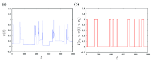
Figure 1: A sample path $v(t)$ exhibits long sticking times whenever the particle is injected to a small velocity. This is due to the trapping mechanism, specifically the vanishing of the collision rate as $R(v)=v^{\alpha}$ for small velocities. Here we use $\alpha=2$ and the parent distribution $f(v)$ is uniform in the interval $(0,1)$. We also show the indicator function which attains the value unity whenever $1/4<v(t)<1$, otherwise it is zero. As explained in the text this observable is always integrable with respect to the infinite density, a trait crucial for infinite ergodic theory.

In this work we are influenced by advances in the statistical theory of optical experiments, in particular single molecule tracking. In this field the removal of the problem of ensemble averaging MoernerOrrit , led to new insights into the applications and limitations of standard ergodic theory, for example in the context of diffusion of single molecules in the cell Review ; Garini and the power-law distributed sojourn times of dark and bright states of blinking quantum dots Kuno ; Stefani . Similarly, here the time averages of a single trajectory of an atom/molecule in the process of laser cooling are studied theoretically, as fits this special issue. As mentioned, the omnipresent power-law distributed sojourn times, are found also in laser cooled gases, and they describe the times in the momentum trap in the vicinity of small velocities. These are responsible for the emergence of the infinite ergodicity framework.

A summary of our main results was published in a recent letter letter , while this paper is organised as follows. We present the model, and analyse the distribution of velocities with a master equation, this gives both a scaling solution and the infinite invariant density, see Sec. II. Sec. III is devoted to a discussion of both, ensemble and time averages, in generality. We then focus on the energy of the system, developing tools for analysing the corresponding paths, see Sec IV. In Sec. V we explore the Darling-Kac phase, where the observable of choice is integrable with respect to the non-normalized state corresponding to $\alpha<3$. We then study the non-integrable phase $3<\alpha$, in Sec. VI. We end with open questions, perspective, and a summary.

II Infinite density and scaling solution

Let $v>0$ be the speed of the atom under the influence of sub-recoil laser cooling. The stochastic process for $v(t)$, presented schematically in Fig. 1, is described by the following rules CT . At time $t=0$ draw the speed $v_{1}$ from the probability density function (PDF) $f(v)$. Momentum is conserved until the atom experiences a jolt due to the interaction with the laser field. Hence the speed of the atom will remain fixed for time $\tilde{\tau}_{1}$. The PDF of $\tilde{\tau}_{1}$ conditioned on $v_{1}$ is exponential

$$q(\tilde{\tau}|v)=\exp[-\tilde{\tau}/\tau(v)]/\tau(v).$$ (1)

Here $\tau(v)$ is the mean lifetime which depends on the speed of the particle. After time $\tilde{\tau}_{1}$ we draw a new speed $v_{2}$ from $f(v)$. The process is then repeated. Namely we now draw the second waiting time $\tilde{\tau}_{2}$ from the PDF in Eq. (1) with an updated lifetime $\tau(v_{2})$. This process is then renewed. Given $f(v)$ and $\tau(v)$ we are interested in the speed of the particle at time $t$. The event of change of velocity is called below a collision or a jump. Here we analyse the velocity distribution using a master equation approach. A different elegant approach to the problem was considered by Bertin and Bardou Bertin using the dynamics of the lifetimes, and this is presented in Appendix A.

Master equation. Let $\rho\left(v,t\right)$ be the PDF of $v$ at time $t$. The repeated cooling process, as described above, leads to an evolution of $\rho\left(v,t\right)$, which is governed by a Master equation

$$\frac{\partial\rho\left(v,t\right)}{\partial t}=\int_{0}^{\infty}\left[W(v^{\prime}\rightarrow v)\rho\left(v^{\prime},t\right)-W(v\rightarrow v^{\prime})\rho\left(v,t\right)\right]{\rm d}v^{\prime}$$ (2)

containing gain and loss terms, respectively. The independence of the parent distribution $f(v^{\prime})$ from the previous velocity value $v$ leads to a factorization of the transition rates from $v$ to $v^{\prime}$

$$W(v\rightarrow v^{\prime})=R(v)f(v^{\prime}).$$ (3)

Using Eq. (3) and the normalization $\int_{0}^{\infty}f(v^{\prime}){\rm d}v^{\prime}=1$ gives

$$\int_{0}^{\infty}W(v\rightarrow v^{\prime}){\rm d}v^{\prime}=R(v),$$ (4)

which identifies $R(v)$ as a jump rate, the rate of leaving the state with velocity $v$, which is the inverse of the lifetime, i.e. $R(v)=1/\tau(v).$ With these assumptions the Master equation Eq. (2) simplifies to

$${\partial{\rho}\over\partial t}=-{\rho\over\tau(v)}+f(v)\int_{0}^{\infty}{\rho(v^{\prime},t)\over\tau(v^{\prime})}{\rm d}v^{\prime}.$$ (5)

An invariant density $\rho^{\ast}\left(v\right)$, which zeros the time derivative on the left hand side of the master equation, is obtained easily from Eq. (2) i.e.

$$\left[W(v^{\prime}\rightarrow v)\rho^{\ast}\left(v^{\prime}\right)-W(v\rightarrow v^{\prime})\rho^{\ast}\left(v\right)\right]=0$$ (6)

leading to $R(v^{\prime})f(v)\rho^{\ast}\left(v^{\prime}\right)=R(v)f(v^{\prime})\rho^{\ast}\left(v\right)$,

which is fulfilled, if e.g. the $v-$dependence on both sides is identical, i.e., if $f(v)=R(v)\rho^{\ast}\left(v\right)C$,  or

$$\rho^{\ast}\left(v\right)=\frac{1}{C}\tau(v)f(v).$$ (7)

and $C$ is some constant. Below we promote two scenarios for this invariant solution of Eq. (5). The first is well known and it is the case when $\rho^{\ast}\left(v\right)$ is normalizable, the second when it is not. We will see below that even if the normalization integral diverges, which happens easily, then non-normalizable density $\rho^{\ast}\left(v\right)$ of Eq. (7) is still meaningful and can be used for calculating certain time and ensemble averages.

The integral in Eq. (5) represents the process where atom’s state $v^{\prime}$ is shifted due to the laser-atom interaction and the new velocity $v$ is drawn from the PDF $f(v)$. In CT a uniform model for $f(v)$ was investigated, and hence (unless stated otherwise) in our examples below we choose $f(v)=1/v_{{\rm max}}$ for $0<v<v_{{\rm max}}$ otherwise it is zero. In equilibrium, we have

$$\rho^{{\rm eq}}(v)={\tau(v)f(v)\over Z}$$ (8)

and the normalisation is $Z=\int_{0}^{\infty}\tau(v)f(v){\rm d}v$. Here the steady state exists in the usual sense and the normalised density $\rho^{{\rm eq}}(v)$ can be used to predict the ensemble and the corresponding time averages of the process. Especially Birkhoff’s Birkhoff ergodic theory states that for an observable ${\cal O}[v(t)]$ the time average is equal to the ensemble average

$$\lim_{t\to\infty}{1\over t}\int_{0}^{t}{\cal O}[v(t^{\prime})]{\rm d}t^{\prime}=\langle{\cal O}(v)\rangle,$$ (9)

where the ensemble average in equilibrium is

$$\langle{\cal O}(v)\rangle=\int_{0}^{\infty}\rho^{{\rm eq}}(v){\cal O}(v){\rm d}v.$$

However, if

$$\tau(v)\sim cv^{-\alpha}\ \ \mbox{ for }\ \ v\to 0$$ (10)

and $\alpha>1$ the above standard framework does not work, since $Z$ diverges. This is precisely the situation for laser cooled atoms where $\alpha=2$ or $\alpha=4,6$ depending on the specific atom-light interaction process CT ; Bertin . Clearly once $v$ becomes small then the lifetime is very long. This is the widely discussed mechanism of sub-recoil cooling, the atoms once slowed down will have a very long lifetime, and hence remain in the cold state for a long time. The atoms thus pile up close to zero velocity. This phase, i.e. $\alpha>1$, is the case where infinite ergodic theory plays a vital role, as we will show.

To solve the problem we consider the long time limit and then for $v\neq 0$ we have CT ; Bertin

$$\rho(v,t)\sim{b\tau(v)f(v)\over t^{1-\tilde{\xi}}}.$$ (11)

This is a quasi-steady state in the sense the numerator is proportional to the usual $\rho^{{\rm eq}}(v)$ Eq. (8). It is valid for $v$ beyond a small layer around $v\simeq 0$, which itself shrinks with time to zero, see below. It is easy to check that Eq. (11) is a valid solution by insertion into Eq. (5). Indeed the time derivative on the left hand side gives $(\tilde{\xi}-1)\rho(v,t)/t$ which is vanishing when $t\to\infty$, and the right hand side gives zero just like for ordinary steady states. Here the exponent $0<\tilde{\xi}<1$ is called the infinite density exponent, and it will be soon determined and similarly for the constant $b$.

The solution Eq. (11) is invalid for very small $v$ because it diverges at $v\to 0$ in such a way that it is non-integrable since $\alpha>1$. Following CT ; Bertin we seek a scaling solution

$$\rho(v,t)\sim t^{\tilde{\gamma}}g(t^{\tilde{\gamma}}v)$$ (12)

which describes the inner region of slow atoms and hence the cooling effect. Here $v\propto 1/t^{{\tilde{\gamma}}}$ and hence the velocity is small since $t$ is large. Of course the inner and outer solutions Eqs. (11,12) must match, and we will exploit this to find the dynamical exponents of this problem $\tilde{\xi}$ and $\tilde{\gamma}$. The latter is what we call the scaling exponent. Using Eq. (11) we have $\rho(v,t)\propto v^{-\alpha}$ for $v\to 0$ and this must match the inner solution hence we have

$$g(x)\propto x^{-\alpha}\ \ \mbox{for}\ x>>1.$$ (13)

Note that $g(x)$ is integrable namely it can be normalised when $\alpha>1$.

We insert Eq. (12) in Eq. (5) to find an equation for $g(x)$. Some thought is required with respect to the upper limit of integration that stretches to infinite velocities on the right hand side of Eq. (5). However, the scaling function does not describe large velocities, in fact velocities of order $v\propto v_{{\rm max}}$ are modelled by the quasi-steady state, Eq. (11), as mentioned. Let us, however, pretend that we do not know this and see how it comes out of the master equation. We recall that $t$ is large, and replace the upper limit of integration over velocity by an upper cutoff $ht^{\beta}$. We call $\beta$ the cutoff exponent. We then find using Eqs. (5) and (12)

$$\tilde{\gamma}t^{\tilde{\gamma}-1}\left[g(t^{\tilde{\gamma}}v)+t^{\tilde{\gamma}}vg^{\prime}(t^{\tilde{\gamma}}v)\right]\simeq-{t^{\tilde{\gamma}}g(t^{\tilde{\gamma}}v)\over\tau(v)}+f(v)\int_{0}^{ht^{\beta}}{t^{\tilde{\gamma}}g(t^{\tilde{\gamma}}v)\over\tau(v)}{\rm d}v,$$ (14)

where $g^{\prime}(x)$ is the derivative of $g$ with respect to $x$. Clearly the natural scaled variable is $x=t^{\tilde{\gamma}}v$. We now realise that only the small $v$ behaviour of $\tau(v)$ determines the properties of the scaling solution and hence $g(x)$. This as already pointed out is because the particles pile up close to zero velocity and hence only the small $v$ limit matters. In contrast note that we need the full structure of $\tau(v)$ to describe the outer solution Eq. (11). Hence now we replace $\tau(v)\rightarrow cv^{-\alpha}$ in Eq. (14) and after change of variables we find

$$\tilde{\gamma}t^{\tilde{\gamma}-1}\left[g(x)+xg^{\prime}(x)\right]=-t^{\tilde{\gamma}-\tilde{\gamma}\alpha}{1\over c}x^{\alpha}g(x)+t^{-\tilde{\gamma}\alpha}f\left({x\over t^{\tilde{\gamma}}}\right)\int_{0}^{ht^{\beta+\tilde{\gamma}}}g(x)x^{\alpha}{\rm d}x.$$ (15)

Recall the large $x$ behaviour of $g(x)$ Eq. (13) which gives $g(x)x^{\alpha}\to\mbox{const}$ and hence we may find the long time limit of the integral in Eq. (15) and get

$$\tilde{\gamma}t^{\tilde{\gamma}-1}\left[g(x)+xg^{\prime}(x)\right]=-t^{\tilde{\gamma}-\tilde{\gamma}a~{}\alpha}~{}{x^{\alpha}g(x)\over c}+{\cal N}t^{\beta+\tilde{\gamma}-\tilde{\gamma}~{}\alpha}.$$ (16)

Here we used $\lim_{t\to\infty}f(x/t^{\tilde{\gamma}})=f(0)$ which is a constant not equal zero, further $f(0)$ is swallowed in ${\cal N}$ with other constants and hence is not presented explicitly in Eq. (16). Eq. (16) should be time independent hence we can find the exponents of the problem, $\tilde{\gamma}\alpha=1$ and $\beta=0$. The latter is expected since the cutoff of velocity is of order $t^{0}$, i.e. $v_{{\rm max}}$. The constant ${\cal N}$ is eventually determined from normalisation, see below.

Figure 2: The scaled PDF of velocity $t^{1-\gamma}\rho(v,t)$ versus $v$ for increasing times as indicated in the figure. A cooling process with a uniform parent velocity PDF $f(v)$ the maximum allowed velocity being unity is considered. The collision rate is $R(v)=v^{2}$ so $\alpha=2$ and hence $\gamma=1/2$. The data in the long time limit converges to the infinite density Eq. (24) presented with a dashed black line.

Figure 3: Similar to Fig. 2 we show the scaled PDF of velocity $t^{1-\gamma}\rho(v,t)$ versus $v$, however, here we simulated a process with an exponential parent velocity PDF $f(v)$ with mean unity, the collision rate is unchanged and hence $\alpha=2$. The data in the long time limit converges to the infinite density Eq. (24) shown as a dashed black line. For finite times, we see expected deviations between the infinite invariant density and the numerical solution, which are obvious and clearly visible for small velocities. For not too large velocities, i.e. velocities much smaller than the mean of $f(v)$, which is $1/2$ in this example, the scaling solution, Eq. (12) with Eq. (19) (red line), nicely matches the data. We see that both, the scaling solution and the infinite density, describe the distribution of velocities, for $t=10^{4}$. For intermediate velocities the two solutions match. Comparing with Fig. 2 we see that the sharp cutoff of the infinite density (due to the uniform PDF of velocities) is replaced here with an exponential decay.

We now use the scaling exponent

$$\gamma\equiv{1\over\alpha}$$ (17)

and from now on $\tilde{\gamma}=\gamma$. This exponent is in the range $0<\gamma<1$, and it describes the fat tail PDF of the waiting time within the momentum trap, $\phi_{1}(\tilde{\tau})\propto\tilde{\tau}^{-1+\gamma}$ (see details below, this PDF is found via averaging the exponential PDF $q(\tilde{\tau}|v)$ from Eq. (1) over the random velocities). Here we see that the mean waiting time diverges, and hence as mentioned in the introduction the process is scale free. Generally, infinite ergodic theory is related to such processes, where the mean of the microscopic time scale diverges.

The scaling function is thus determined by the following equation

$$\gamma\left[g(x)+xg^{\prime}(x)\right]=-{x^{1/\gamma}g(x)\over c}+{\cal N}.$$ (18)

The substitution $y(x)=xg(x)$ helps simplifying this equation even further, and eventually the solution reads CT

$$g(x)={{\cal N}\over\gamma x}\exp\left(-{x^{1/\gamma}\over c}\right)\int_{0}^{x}\exp\left({z^{1/\gamma}\over c}\right){\rm d}z.$$ (19)

With the help of the generalized Dawson integral $F(p,x)=\exp(-x^{p})\int\limits_{0}^{x}\exp(y^{p})\rm{d}y$, which according to Dawson can be expressed by the confluent hypergeometric function $M(a,b,z)$, the scaling function can be written as $g(x)=\frac{N}{\gamma}\frac{c^{\gamma}}{x}F(\frac{1}{\gamma},\frac{x}{c^{\gamma}})=\frac{N}{\gamma}M(1,1+\gamma,-\frac{x^{1/\gamma}}{c})$, which agrees with the result in CT . ${\cal N}$ is determined from normalization $\int_{0}^{\infty}g(x){\rm d}x=1$ and we find from formula $7.612(1)$ from GRAD

$$\frac{{\cal N}}{\gamma}=\frac{1}{\Gamma(1+\gamma)}\frac{\sin(\pi\gamma)}{\pi\gamma}{1\over c^{\gamma}}.$$ (20)

As announced, the infinite density exponent $\tilde{\xi}$ can be found by matching the inner and outer solution. Specifically the left part of the outer solution Eq. (11) is $\rho(v,t)\propto v^{-\alpha}/t^{1-\tilde{\xi}}$ is matched with the right part of the inner solution Eqs. (12,13) give $\rho(v,t)\propto v^{-\alpha}/t^{1-\gamma}$. resulting in

$$\tilde{\xi}=\gamma.$$ (21)

Given ${\cal N}$ in Eq. (20) we can determine $b$ in Eq. (11). Using integration by parts Eq. (19) Dawson yields $g(x)\sim{\cal N}c/x^{1/\gamma}$ for $x\to\infty$. So from the scaling solution Eq. (12) we have for large $x=vt^{\gamma}$,

$$\rho(v,t)\sim{{\cal N}c\over t^{1-\gamma}v^{1/\gamma}}.$$ (22)

This is matched to the small $v$ behaviour of the infinite density solution Eq. (11) which gives using Eq. (10)

$$\rho(v,t)\sim{bf(0)c\over t^{1-\gamma}}{1\over v^{1/\gamma}}.$$ (23)

Thus we find the constant $b$ given by $bf(0)={\cal N}$.

To summarise we find that

$$\boxed{\lim_{t\to\infty}t^{1-\gamma}\rho(v,t)={\cal N}\tau(v){f(v)\over f(0)}={\cal I}_{v}(v).}$$ (24)

The function ${\cal I}_{v}(v)$ is non-normalisable since ${\cal I}_{v}(v)\propto v^{-1/\gamma}$ for $v\to 0$ and $1/\gamma=\alpha>1$. This is why it is called an infinite density. The non-normalizability is hardly surprising since we take a perfectly normalised PDF $\rho(v,t)$ and multiply it by $t^{1-\gamma}$ hence the area under the product will diverge in the long time limit. Still the function ${\cal I}_{v}(v)$ can be used to calculate ensemble and time averages, as we will show below.

Figs. 2,3 demonstrate the main results of this section using finite time simulations of the process. In Fig. 2 simulations are presented for the uniform velocity PDF $f(v)$ and we use $v_{\rm max}=1$ while for the rate function we use $c=1$. Unless stated otherwize these parameters will be used in all the figures of this paper. In Fig. 3 we show the case where the parent velocity distribution is exponential. While the scaling solution is not sensitive to the shape of $f(v)$, the infinite density is, as demonstrated in the figures.

The distribution for very small velocity is described by Eq. (12) with the scaling function $g(x)$, Eq. (19). This scaling solution as a stand alone is not a sufficient description of a cooled system for the following reason. From Eqs. (12,13) we have $\rho(v,t)\propto v^{-\alpha}$ for large $v$ and for now let us focus on the realistic choice $\alpha=2$. We find the awkward situation that the second moment of $v$, namely the mean kinetic energy would be infinite, due to the fat-tail of the solution, which is not what we expect from a cold system. Thus the scaling solution $g(x)$ describes the pile up of particles close to zero velocity, but it also exhibits an unexpected heavy power law tail for large velocities. The infinite density describing the outer region cures this problem, in the sense that it describes the large velocity cutoff, see Figs. 2,3. From here we see that for calculating, for instance the mean kinetic energy, we need the infinite density ${\cal I}_{v}(v)$. The technical details of this calculation will be presented below. Further, while the scaling function cures the non-normalisable trait of the infinite density which stems from its small $v$ behaviour, we find that also the complement is true: the infinite density cures the unphysical divergence of the kinetic energy, found using the scaling solution, which is due to its unphysical large $v$ properties. In short we need both tools to describe the velocity distribution.

Finally, there is experimental evidence for the scaling solution. According to Eq. (12) the width of the velocity distribution, is proportional to $t^{-\gamma}$ and hence to $t^{-1/\alpha}$ Reichel ; CT1 . Experimentally one may control the shape of the rate function $R(v)=1/\tau(v)$ in the vicinity of zero, and engineered experiments provided the values $\alpha=2$ and $\alpha=4$. Note that $\alpha=2$ corresponds to an analytical expansion of $R(v)\propto v^{2}$ around its minimum at $v=0$. Hence the theory Eq. (12) predicts that the full width at half maximum of the velocity PDF decays like $t^{-1/2}$ for $\alpha=2$ and as $t^{-1/4}$ for $\alpha=4$. Both these behaviours were indeed observed experimentally, up to times of order $20$ milliseconds, which given the lifetime of the atom, is considered very long in this field. This cooling experiment from $1995$, using Cesium, reports below $3$ nano-Kelvin temperatures and due to the non-Gaussian nature of the momentum packet, temperature is defined by the width of the momentum distribution and not by its variance. This reality is also consistent with quantum Monte Carlo simulations CT . In a later experiment, the momentum distribution of Helium was recorded in full agreement with the statistical method CT ; Saubamea . As far as we know, so far, the infinite density was not explored experimentally.

III Ensemble and time averages

We now consider the long time limit of averaged observables, the latter denoted ${\cal O}[v(t)]$, so the observable is a function of the stochastic process $v(t)$. In usual statistical physics both, the ensemble average and the time average of such observables, are investigated and we do the same here. Examples are the indicator function ${\cal O}[v(t)]=I[v_{a}<v(t)<v_{b}]$ and the kinetic energy of the particle ${\cal O}[v(t)]=v^{2}(t)=E_{k}(t)$ and $m/2=1$ with $m$ the mass of the atom. The indicator function equals unity, if the condition $v_{a}<v(t)<v_{b}$ is true, otherwise it is zero, namely it is an observable that switches at random times between $1$ and $0$, thus this observable represents a dichotomous process, see Fig. 1. The kinetic energy $E_{k}(t)$ is an observable that needs no introduction. The ensemble average is

$$\langle{\cal O}(t)\rangle=\int_{0}^{\infty}{\cal O}(v)\rho(v,t){\rm d}v$$ (25)

and hence we find using Eq. (24)

$$\lim_{t\to\infty}t^{1-\gamma}\langle{\cal O}(v)\rangle=\int_{0}^{\infty}{\cal O}(t){\cal I}_{v}(v){\rm d}v.$$ (26)

In this sense the infinite invariant density ${\cal I}_{v}(v)$ replaces the standard invariant density $\rho^{{\rm eq}}(v)$. The formula is valid provided that the integral is finite and such an observable ${\cal O}(v)$ is called integrable with respect to the infinite density. Examples are the indicator function and the kinetic energy

$$\lim_{t\to\infty}t^{1-\gamma}\langle I(v_{a}<v(t)<v_{b})\rangle=\int_{v_{a}}^{v_{b}}{\cal I}_{v}(v){\rm d}v,\ \ \ \mbox{and}\ \ \ \ \lim_{t\to\infty}t^{1-\gamma}\langle E_{k}(t)\rangle=\int_{0}^{\infty}v^{2}{\cal I}_{v}(v){\rm d}v\ \ \mbox{for}\ \ \alpha<3.$$ (27)

The former shows that the number of particles in the interval $v_{a}<v<v_{b}$ is shrinking in time, provided that $0<v_{a}$ and the latter indicates that the energy of the system is decaying similarly, like $\langle I(v_{a}<v(t)<v_{b})\rangle\propto\langle E_{k}(t)\rangle\propto 1/t^{1-\gamma}$. Since ${\cal I}_{v}(v)\propto v^{-\alpha}$ for $v\to 0$ we see that the second integral exists only when $\alpha<3$, hence the kinetic energy is an integrable observable only if $\alpha<3$. If this condition does not hold, the kinetic energy is called a non-integrable observable and then other rules apply, see below. Roughly speaking integrable observables cure the non-normalisable trait of the infinite density found for $v\to 0$, and importantly these integrable observables are very basic to physical systems, for example the energy.

We now consider the time average of an integrable observable

$$\overline{{\cal O}}(t)={1\over t}\int_{0}^{t}{\cal O}[v(t^{\prime})]{\rm d}t^{\prime}.$$ (28)

In standard ergodic theory $\lim_{t\to\infty}\overline{{\cal O}}(t)=\langle{\cal O}\rangle_{{\rm eq}}$. In the current case the dimensionless variable $\Upsilon=\gamma\overline{O}(t)/\langle{\cal O}(t)\rangle$ remains random in the long time limit and as shown below it satisfies the Darling-Kac theorem Darling provided the observable is integrable. Here the mean of $\Upsilon$ in the long measurement time limit is unity and importantly in that limit its PDF is time independent. First let us consider the ensemble mean, namely we consider an ensemble of paths and average over time and then over the ensemble

$$\langle{\overline{\cal O}}(t)\rangle=\left\langle{1\over t}\int_{0}^{t}{\cal O}[v(t^{\prime})]{\rm d}t^{\prime}\right\rangle={1\over t}\int_{0}^{t}\int_{0}^{\infty}{\cal O}(v)\rho(v,t^{\prime}){\rm d}v{\rm d}t^{\prime}.$$ (29)

Here we switched the order of the time and ensemble averages. Considering the long time limit and using Eq. (24)

$$\boxed{\langle{\overline{\cal O}}(t)\rangle\sim{1\over t}\int_{0}^{t}{\rm d}t^{\prime}{\int_{0}^{\infty}{\cal O}(v){\cal I}_{v}(v){\rm d}v\over t^{\prime 1-\gamma}}={\int_{0}^{\infty}{\cal O}(v){\cal I}_{v}(v){\rm d}v\over\gamma t^{1-\gamma}}}$$ (30)

where we used $0<\gamma<1$. Hence we conclude that

$$\boxed{\lim_{t\to\infty}{\langle\overline{\cal O}(t)\rangle\over\langle{\cal O}(t)\rangle}={1\over\gamma}.}$$ (31)

Thus we established a relation between the time average and the ensemble average. The latter is obtained using the infinite density ${\cal I}_{v}(v)$ and thus this invariant density is not merely a tool for the calculation of the ensemble average but rather it gives also information on the time average. More precisely as discussed below $\Upsilon$ exhibits universal statistics independent of the observable, provided that it is an integrable observable. The $1/\gamma$ factor in Eq. (31) stems from the time averaging and for example if $\alpha=1/\gamma=2$ we have $\langle\overline{{\cal O}}(t)\rangle\sim 2\langle{\cal O}(t)\rangle$, or since both sides of this equation actually go to zero, a more refined statment is $\lim_{t\to\infty}\langle\overline{{\cal O}}(t)\rangle/\langle{\cal O}(t)\rangle=2$.

IV Kinetic energy

We consider the time average of the kinetic energy of the atom

$$\overline{E}_{k}(t)=\overline{v^{2}}(t)={1\over t}\int_{0}^{t}v^{2}(t^{\prime}){\rm d}t^{\prime}$$ (32)

in the limit of long times. While we focus on a particular observable, the theory presented below is actually rather general. As mentioned, depending on the value of $\alpha$, the observable $v^{2}(t^{\prime})$ can be either integrable with respect to the infinite density, or not. Hence, here we will develop a general theory, for the time averages, valid in principle wether the observable is integrable or not. To do so, we use tools from random walk theory MetzKlaf ; Kutner , in particular certain types of Lévy walks Denisov ; Shinkai ; Albers .

We focus on the numerator of Eq. (32) which is a functional of the velocity path,

$${\cal S}(t)=\int_{0}^{t}v^{2}(t^{\prime}){\rm d}t^{\prime}.$$ (33)

Since we have no potential energy, ${\cal S}(t)$ is the action, which is increasing with time and $\overline{E}_{k}(t)={\cal S}(t)/t$. Since the speed of particle is a constant between collision events

$${\cal S}(t)=\sum_{i=1}^{N(t)}(v_{i})^{2}\tilde{\tau}_{i}+(v_{N(t)+1})^{2}t_{B}(t).$$ (34)

Here $v_{1}$ is the velocity drawn at the start of the process, $v_{2}$ the velocity drawn after the first collision, etc. The times $\tilde{\tau}_{i}$ are the times between collision events. $t_{B}(t)$ is the time elapsing between measurement time $t$ and the last event in the sequence, also called the backward recurrence time Godreche2001 ; Wanli . Here we have the constraint

$$\sum_{i=1}^{N(t)}\tilde{\tau}_{i}+t_{B}(t)=t,$$ (35)

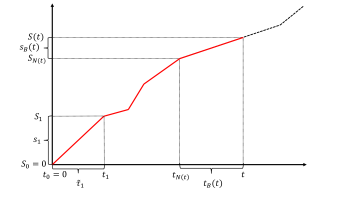
Figure 4: Action-time diagram illustrating the generalized Lévy walk performed by the action ${\cal S}(t)$, Eq. (38). $t_{N(t)}$ and ${\cal S}_{N(t)}$ are the partial sums appearing in Eqs. (35) and (38), where $t_{B}(t)=t-t_{N(t)}$ and $s_{B}(t)=S(t)-S_{N(t)}$ are the backward recurrence time and the associated action increment, respectively. For this sample trajectory the number $N(t)$ of renewals until time $t$ is $N(t)=4$.

see schematics in Fig. 4. Finally, $N(t)$ is the random number of collisions until time $t$.

Recall, that at each collision event we draw $v_{i}$ from the parent PDF $f(v)$ and then the waiting time $\tilde{\tau}_{i}$ from Eq. (1) $q(\tilde{\tau}|v_{i})=R(v_{i})\exp[-\tilde{\tau}R(v_{i})]$, which is the conditional PDF of the waiting time, given a velocity $v_{i}$. Hence the waiting times are not identically distributed, unless the rate is a constant. Further in this section we will assume that

$$f(v)={1\over v_{{\rm max}}}\ \ \mbox{when}\ \ 0<v<v_{{\rm max}}$$ (36)

and zero otherwise. Thus we consider a uniform distribution of the speed, and further the rate is

$$R(v)={v^{\alpha}\over c}$$ (37)

which is the inverse of the mean decay time $\tau(v)$ in Eq. (10). Here $c$ is a constant with units of time times speed to the power of $\alpha$.

We may write $s_{i}=(v_{i})^{2}\tilde{\tau}_{i}$ and similarly $s_{B}(t)=(v_{N(t)+1})^{2}t_{B}(t)$ and then

$${\cal S}(t)=\sum_{i=1}^{N(t)}s_{i}+s_{B}(t).$$ (38)

At first this appears to be a problem of the summation of $N$ random variables, which is classical in many fields, in particular in the theory of random walks. However, here $N(t)$ is random, and is determined by the sequence of waiting times, which in turn are correlated with the jump size, i.e. the increments of $s_{i}$ of of ${\cal S}(t)$ Eq. (38) and also the $\tau_{i}$s in Eq. (35) are constrained by the measurement time $t$. In particular when $\alpha>1$ the statistics is very different from normal.

Remark: In what sense are we dealing here with a generalized Lévy walk? The simplest form of the Lévy walk deals with the displacement of a particle $-\infty<X(t)<\infty$ which is given by $X(t)=\sum_{i}^{N(t)}v_{i}\tilde{\tau_{i}}+v_{N+1}t_{B}(t)$. Here the velocity $v_{i}$ is say either $+1$ or $-1$ with probability half (unbiased random walk) while the travel time PDF is fat tailed. In our study $S(t)>0$ plays a role similar to $X(t)$ of a biased Lévy walk. The main difference is the following. For standard Lévy walks the distribution of the flight times $\tilde{\tau}$ is independent from the value of the velocity, i.e. the joint PDF of velocity and travel times is a product of the marginal PDFs. Here, we have a different situation, as the velocity of the atom after the jump event is correlated with the random time of flight by a law determined with $R(v)=1/\tau(v)$. However, as stated in the abstract, the action $S(t)$ is performing a generalised type of Lévy walk, which is analysed below.

IV.1 PDF of action increments and waiting times

The joint PDF of $s,\tilde{\tau}$ and $v$ is

$$\phi_{3}(s,\tilde{\tau},v)=\delta(s-v^{2}\tilde{\tau})q(\tilde{\tau}|v)f(v)$$ (39)

where $f(v)$ and $q(\tilde{\tau}|v)$ are defined in Eqs. (1,36) respectively. Here the delta function comes from the definition of one step, i.e. given a specific velocity and waiting time the increment of the action is fixed. The subscript $3$ indicates that we are dealing here with three random variables. We already mentioned that the action increments and the waiting times are correlated and hence to solve the problem we need the joint PDF of $s$ and $\tilde{\tau}$. This is obtained from integration of Eq. (39) over $v$ which gives

$$\phi_{2}(s,\tilde{\tau})={1\over 2v_{{\rm max}}\sqrt{s\tilde{\tau}}}R\left(\sqrt{{s\over\tilde{\tau}}}\right)\exp\left[-\tilde{\tau}R\left(\sqrt{{s\over\tilde{\tau}}}\right)\right]$$ (40)

when $0\leq s\leq v_{{\rm max}}^{2}\tilde{\tau}$ and if this condition is not valid, the joint PDF is equal zero. In the context of random walk theory such joint distributions are investigated in the context of coupled continuous time random walks Denisov ; Albers ; KBS ; Miya1PRE ; Miya2JSP ; Aghion since the increment $s$ and waiting times $\tilde{\tau}$ are correlated,

Further integrating over $s$ we get the marginal PDF of the waiting times.

$$\phi_{1}(\tilde{\tau})={c^{1/\alpha}\over\alpha v_{{\rm max}}}\tilde{\tau}^{-1-1/\alpha}\gamma\left(1+{1\over\alpha},{v_{{\rm max}}^{\alpha}\tilde{\tau}\over c}\right),$$ (41)

where $\gamma(.,.)$ is the lower incomplete Gamma function. For large $\tilde{\tau}$ we get a power law decay

$$\phi_{1}(\tilde{\tau})\sim\mbox{const}\ \tilde{\tau}^{-1-1/\alpha}$$ (42)

hence if $\alpha>1$ the mean waiting time diverges and $\mbox{const}=c^{1/\alpha}\Gamma(1+1/\alpha)/(\alpha v_{{\rm max}})$. As is well known WEB ; Review the divergence of the mean waiting time signals special ergodic properties, since no matter how long we measure we cannot exceed the mean time, and hence ergodicity in its usual sense is broken. At short waiting times we have $\phi_{1}(\tilde{\tau})\sim v_{{\rm max}}^{\alpha}/[(1+\alpha)c]$.

The marginal PDF of the action increment is found integrating Eq. (39) over $\tilde{\tau}$ and $v$. We use the notation that the argument in the PDF defines the variable under study and in this case it is easy to show that

$$\phi_{1}(s)={1\over v_{{\rm max}}}\int_{0}^{v_{{\rm max}}}{v^{\alpha-2}\over c}\exp\left(-{v^{\alpha-2}s\over c}\right){\rm d}v.$$ (43)

Then for the example $\alpha=2$ we find $\phi_{1}(s)=\exp(-s/c)/c$, namely an exponential decay. More generally the mean of the action increments $\langle s\rangle=\int_{0}^{\infty}s\phi_{1}(s){\rm d}s$ is an important quantifier and Eq. (43) gives

$$\langle s\rangle=\left\{\begin{array}[]{c c}{cv_{{\rm max}}^{2-\alpha}\over 3-\alpha}&\alpha<3\\ \infty&\alpha>3\end{array}\right..$$ (44)

Clearly the mean diverges when $\alpha>3$ which is critical for our discussion. Note the peculiarity of the case $\alpha=2$ as the mean action increment is independent of $v_{{\rm max}}$.

We now examine the distribution of $s$ in some detail. For $\alpha>2$ we change variables according to $z=v^{\alpha-2}s/c$ in Eq. (43) and then the lower limit of the integral namely $v=0$ corresponds to $z=0$. Note that when $\alpha<2$ the lower limit of integration over $z$ transform to infinity. We find

$$\phi_{1}(s)={c^{1\over\alpha-2}\over(\alpha-2)v_{{\rm max}}}s^{-1-{1\over\alpha-2}}\gamma\left({\alpha-1\over\alpha-2},{v_{{\rm max}}^{\alpha-2}s\over c}\right)\ \ \ \mbox{when}\ \ \ \alpha>2.$$ (45)

For large $s$ the lower incomplete Gamma function is a constant equal to the corresponding Gamma function, hence for large $s$ we find the power law tail $\phi_{1}(s)\propto s^{-1-1/(\alpha-2)}$ and from here we see again that when $\alpha>3$ the mean action increment diverges. For example for the experimentally relevant case $\alpha=4$ we have

$$\phi_{1}(s)={c^{1\over 2}\over 2v_{{\rm max}}}s^{-3/2}\gamma\left({3\over 2},{v_{{\rm max}}^{2}s\over c}\right)\ \ \ \mbox{for}\ \ \alpha=4$$ (46)

which gives $\phi_{1}(s)\sim\sqrt{c\pi}/(4v_{{\rm max}})s^{-3/2}$ when $s\to\infty$.

For $\alpha<2$ the integral Eq. (43) can be solved similarly and the solution can be expressed in terms of the upper incomplete Gamma function

$$\phi_{1}(s)={c^{1\over\alpha-2}\over v_{{\rm max}}(2-\alpha)}s^{-1-{1\over\alpha-2}}\Gamma\left({\alpha-1\over\alpha-2},{(v_{{\rm max}})^{\alpha-2}s\over c}\right),\ \ \ \mbox{when}\ \ \ \alpha<2.$$ (47)

Now for large $s$ the distribution $\phi_{1}(s)$ has an exponential cutoff for all $\alpha$ with $1\leq\alpha\leq 2$, as can be seen from the asymptotic expansion of the upper incomplete Gamma function $\Gamma(a,x)\sim x^{a-1}\exp(-x)$ resulting for $1\leq\alpha<2$ in

$$\phi_{1}(s)\sim\frac{1}{2-\alpha}\frac{1}{s}\exp(-\frac{s}{c}v_{{\rm max}}^{\alpha-2}),$$

and for $\alpha=2$ we saw already that $\phi_{1}(s)=\frac{1}{c}\exp(-\frac{s}{c})$. For small $s$ one gets a finite value $\phi_{1}(s\rightarrow 0)=\frac{v_{0}^{\alpha-2}}{c(\alpha-1)}$ for all $\alpha>1$. The case $\alpha=1$ is special in this respect, because here $\phi_{1}(s)$ is given by

$$\phi_{1}(s)\sim\frac{1}{cv_{{\rm max}}}\Gamma(0,\frac{s}{cv_{{\rm max}}}),$$

which blows up at small $s$ like $\phi_{1}(s)\sim[-\ln(s/(v_{{\rm max}}c))-\gamma_{1}]/(v_{{\rm max}}c)$ where $\gamma_{1}\simeq 0.577$ is the Euler Mascheroni constant. We see that $\alpha=1$, which marks the transition between phases with and without a finite mean waiting time, also exhibits a transition from a blow up at the origin of $\phi_{1}(s)$ to the case where the PDF of increments is a constant at short $s$.

To summarize, we see that the critical value $\alpha=1$ marks the transition from a finite mean waiting to an infinite mean, while $\alpha=3$ marks the transition between a finite mean action increment to a diverging one. The critical value $\alpha=3$ is specific to the observable under study, namely the energy of the atom. Considering an observable like $v(t)^{q}$ and $q\neq 2$ would yield other values of the critical exponent. Still, energy is a basic concept for thermodynamics, so we focus on this particular observable. Also $\alpha=2$ marks a transition, from a power law to an asymptotically exponentially decaying distribution of action increments. However, this does not play an essential role in our investigations of ergodic properties of the process. Importantly, the joint PDF of $s$ and $\tilde{\tau}$ does not factorise, and hence we need to treat the correlations between these variables, which is what is done in the next subsection.

IV.2 Governing Montroll-Weiss equations for the distribution of the total action

We will now investigate the formalism giving the PDF of the action ${\cal S}(t)$ at time $t$ which is denoted $P({\cal S},t)$. In the next subsection we consider some of its long time properties. This density is of course normalised according to $\int_{0}^{\infty}P({\cal S},t){\rm d}{\cal S}=1$. From the relation $\overline{E}_{k}(t)={\cal S}(t)/t$, then from the distribution of ${\cal S}(t)$ we can gain insights on the ergodic properties of $\overline{E}_{k}(t)$.

Let $Q_{N}({\cal S},t){\rm d}t$ be the probability that the $N$-th transition event takes place in the small interval $(t,t+{\rm d}t)$ and the value of the action ${\cal S}(t)$ switched to ${\cal S}$. It is given by the iteration rule

$$Q_{N+1}\left({\cal S},t\right)=\int_{0}^{{\cal S}}\int_{0}^{t}{\rm d}s{\rm d}\tilde{\tau}Q_{N}\left({\cal S}-s,t-\tilde{\tau}\right)\phi_{2}(s,\tilde{\tau})$$ (48)

with $Q_{0}({\cal S},t)=\delta({\cal S})\delta(t)$ being the initial condition. The equation describes the basic property of the process: to arrive in ${\cal S}$ at time $t$ when the previous collision event took place at time $t-\tilde{\tau}$, the previous value of the action was ${\cal S}-s$. Solving this equation is made possible with the convolution theorem of the Laplace transform. Let

$$\hat{Q}_{N}\left(u,p\right)=\int_{0}^{\infty}\int_{0}^{\infty}{\rm d}{\cal S}{\rm d}t\exp\left(-u{\cal S}-pt\right)Q_{N}\left({\cal S},t\right).$$ (49)

be the double Laplace transform of $Q_{n}({\cal S},t)$ where $u\leftrightarrow{\cal S}$ and $p\leftrightarrow t$ are Laplace pairs. Then from the convolution theorem we have

$$\hat{Q}_{N}(u,p)=\left[\hat{\phi}_{2}(u,p)\right]^{N}$$ (50)

where $\hat{\phi}_{2}(u,p)$ is the double Laplace transform of $\phi_{2}(s,\tilde{\tau})$. The PDF $P({\cal S},t)$ is in turn given by

$$P\left({\cal S},t\right)=\sum_{N=0}^{\infty}\int_{0}^{\cal S}\int_{0}^{t}{\rm d}s{\rm d}t^{\prime}_{B}Q_{N}\left({\cal S}-s,t-t^{\prime}_{B}\right)\Phi_{2}\left(s,t^{\prime}_{B}\right).$$ (51)

Here we sum over the number of events $N$ in the time interval $(0,t)$ and take into consideration that the measurement time $t$ is in an interval straddled by two collision events, we further integrate over the backward recurrence time $t^{\prime}_{B}$. Finally, the statistical weight function is

$$\Phi_{2}(s,t^{\prime}_{B})=\int_{t^{\prime}_{B}}^{\infty}{\rm d}\tilde{\tau}\int_{0}^{v_{{\rm max}}}{{\rm d}v\over v_{{\rm max}}}R(v)\exp\left(-R(v)\tilde{\tau}\right)\delta\left(s-t^{\prime}_{B}v^{2}\right).$$ (52)

Here the waiting time for the next jump is larger than $t^{\prime}_{B}$ since by definition the next transition takes place at times larger than $t$. In this equation we average over the speed i.e. integrate over $v$, draw the waiting time from an exponential PDF with a velocity dependent rate and take into consideration the fact that the last increment of the action is given by $s=t^{\prime}_{B}v^{2}$ leading to the delta function.

Now we consider the double Laplace transform of $P({\cal S},t)$ which is denoted by $\hat{P}(u,p)$. We again use the convolution theorem, and Eqs. (50,51) give, after summing a geometric series,

$$\hat{P}(u,p)={\hat{\Phi}_{2}(u,p)\over 1-\hat{\phi}_{2}(u,p)}.$$ (53)

In the context of random walk theory, such a formula is called the Montroll-Weiss equation MW , though typically instead of a double Laplace transform one invokes a Laplace-Fourier transform KBS ; Aghion . In general to invert such an expression to the ${\cal S},t$ domain is hard, however, certain long time limits can be obtained. In particular from the definition of the Laplace transform the mean of the action in Laplace space is

$$\langle\hat{{\cal S}}(p)\rangle=-{\partial\hat{P}(u,p)\over\partial u}|_{u=0}.$$ (54)

Hence to get $\langle{\cal S}(t)\rangle$ we need to deal with a single inverse Laplace transform from $p$ back to $t$. Using Eq. (53) we find

$$\langle\hat{{\cal S}}(p)\rangle=-{{\partial\hat{\phi_{2}}(u,p)\over\partial u}|_{u=0}\hat{\Phi}_{2}(0,p)\over\left[1-\hat{\phi}_{2}(0,p)\right]^{2}}-{{\partial\hat{\Phi}_{2}\left(u,p\right)\over\partial u}|_{u=0}\over 1-\hat{\phi}_{2}(0,p)}.$$ (55)

Note that the double Laplace transform $\hat{\phi}_{2}(0,p)$ evaluated at $u=0$ is merely the Laplace $\tilde{\tau}\to p$ transform of the waiting time PDF $\phi_{1}(\tilde{\tau})$, so $\hat{\phi}_{2}(0,p)=\hat{\phi}_{1}(p)$. This of course comes from the fact that by integration of the joint PDF $\phi_{2}(s,\tilde{\tau})$ over $s$ we obtain the marginal PDF $\phi_{1}(\tilde{\tau})$. The second expression on the right hand side of Eq. (55) is a contribution to the total action from the backward recurrence time, and in the long time limit and for ordinary processes, with a finite mean waiting time, can be neglected. To investigate ergodicity one needs to go beyond the mean and consider the full distribution of ${\cal S}(t)$, or at least its variance.

IV.3 Energy is an integrable observable when $1<\alpha<3$

We now obtain $\langle\overline{E}_{k}(t)\rangle$ using two approaches, the first is based on the Montroll-Weiss machinery Eq. (53), the second exploits the infinite invariant density. When $\alpha<1$ we have a standard steady state since then the mean waiting time is finite. We now consider the case $1<\alpha<3$. According to Eq. (42) the mean waiting time diverges while Eq. (44) yields a finite mean action increment $\langle s\rangle$. Further the observable $v^{2}$, representing the energy, is integrable with respect to the infinite density. This is because ${\cal I}_{v}(v)\propto v^{-\alpha}$ for $v\to 0$, and hence the integral $\int_{0}^{\infty}{\cal I}_{v}(v)v^{2}{\rm d}v$ is finite when $\alpha<3$.

We are interested in the long time limit of $\langle{\cal S}(t)\rangle$, and in Appendix $B$ we derive a rather intuitive equation

$$\langle{\cal S}(t)\rangle\sim\langle N(t)\rangle\langle s\rangle\ \ \ \mbox{and}\ \ \ \ \langle\overline{E}_{k}(t)\rangle\sim{\langle N(t)\rangle\langle s\rangle\over t}$$ (56)

with $\langle N(t)\rangle$ the mean number of collisions in the time interval $(0,t)$. The mean $\langle N(t)\rangle\propto t^{1/\alpha}$ increases sub-linearly because the mean time interval between collision events diverges. This can be justified with a hand waving argument as follows. When the mean $\langle\tilde{\tau}\rangle$ is finite we expect from the law of large numbers that $\langle N(t)\rangle\sim t/\langle\tilde{\tau}\rangle$. However, in our case, when $\alpha>1$ the denominator diverges, and is replaced with the effective mean, namely $\langle N(t)\rangle\propto t/\int_{0}^{t}t^{\prime}\phi_{1}(t^{\prime}){\rm d}t^{\prime}\propto t^{1/\alpha}$. Using well known formulas from renewal theory, briefly recapitulated in Appendix B, we find

$$\langle{\cal S}(t)\rangle\sim\underbrace{{c(v_{{\rm max}})^{2-\alpha}\over 3-\alpha}}_{\langle s\rangle}\underbrace{{\alpha\sin(\pi/\alpha)\over\pi\Gamma\left(1+{1\over\alpha}\right)}\left({(v_{{\rm max}})^{\alpha}t\over c}\right)^{1/\alpha}}_{\langle N(t)\rangle}.$$ (57)

This gives the mean of the time averaged kinetic energy of the particles (mass $m/2=1$) $\langle\overline{E}_{k}(t)\rangle\sim\langle{\cal S}(t)\rangle/t$.

IV.3.1 Infinite ergodic theory at work

Infinite ergodic theory makes the calculation of $\langle E_{k}(t)\rangle$ or $\langle\overline{E}_{k}(t)\rangle$ easy in the sense that one needs only the knowledge of the invariant density ${\cal I}_{v}(v)$. Eqs. (24, 36, 37) give

$${\cal I}_{v}(v)=\left\{\begin{array}[]{c c}{\sin\pi\gamma\over\pi\Gamma(1+\gamma)}c^{1-\gamma}v^{-1/\gamma}&\ 0<v<v_{{\rm max}}\\ 0&\ \mbox{otherwise,}\end{array}\right.$$ (58)

which is clearly non-normalisable. Then the ensemble average Eq. (26)

$$\boxed{\langle E_{k}(t)\rangle=\langle v^{2}(t)\rangle\sim{\int_{0}^{v_{{\rm max}}}v^{2}I_{v}(v){\rm d}v\over t^{1-\gamma}}={\sin(\pi\gamma)\over\Gamma(1+\gamma)\pi}{(v_{{\rm max}})^{3-1/\gamma}\over 3-1/\gamma}\left({c\over t}\right)^{1-\gamma}}$$ (59)

and Eq. (31) gives $\langle\overline{E}_{k}(t)\rangle=\langle E_{k}(t)\rangle/\gamma$. On the other hand $\langle\overline{E}_{k}(t)\rangle=\langle{\cal S}(t)\rangle/t$ and as expected Eq. (57) divided by $\gamma$ gives the same results as in Eq. (59). The calculation using infinite ergodic theory is straight forward and is essentially similar to the averaging we perform with ordinary equilibrium calculations and in that sense it provides a tool more convenient compared to the Montroll-Weiss random walk approach. Of course, the latter yields insights since it connects the mean of the observable to the number of renewals $\langle N(t)\rangle$. Note that as $\gamma\to 1/3$ Eq. (59) exhibits a blow up, further $\lim_{\gamma\to 1/3}v^{3-1/\gamma}=1$ and in this sense the energy is switching to a behaviour that is $v_{{\rm max}}~{}$ independent, more generally it is independent of the parent velocity PDF $f(v)$. This marks the transition to the phase where the energy is no longer an integrable observable, as discussed in Sec. VI below.

Figure 5: To investigate the ergodic properties of the system, we simulate the cooling process model with a uniform velocity distribution $f(v)$ with maximum velocity unity $v_{{\rm max}}=1$, and and the rate $R=v^{\alpha}$ so $c=1$. We then follow velocity paths as a function of time and from each path we obtain the time the particle spent in an interval $v_{a}<v<v_{b}$. Namely, our observable is the indicator function. For standard ergodic processes, e.g. for the velocity of a gas particle obeying Maxwell statistics, this time divided by a long measurement time is approaching the probability of being in the mentioned velocity domain. For the laser cooling model, this time average fluctuates, the Mittag-Leffler distribution describes the corresponding statistics. Specifically we show the histogram of the normalised random variable $\Upsilon=\int_{0}^{t}I(v_{a}<v(t^{\prime})<v_{b}){\rm d}t^{\prime}/\langle\int_{0}^{t}I(v_{a}<v(t^{\prime})<v_{b}){\rm d}t^{\prime}\rangle$ which perfectly matches the theory Eq. (69). Here $\alpha=1.25$ so $\gamma=0.8$, namely we are not too far from the ergodic phase $(\gamma=1)$, hence we see a peak in the distribution of $\Upsilon$ close to its mean which is unity. For ergodic process we will find a delta peak centred on unity and this can be found in our model by choosing $\alpha<1$. We used $t=10^{9}$, $v_{a}=0.4$ and $v_{b}=1$.

V Fluctuations described by the Darling-Kac theorem

We now consider the fluctuations of the time average of the energy for $1<\alpha<3$. Since $\overline{E_{k}}={\cal S}(t)/t$, we investigate the distribution of ${\cal S}(t)$ for long times namely $P({\cal S},t)$, using its double Laplace transform Eq. (53). From Eqs. (36, 37,39) and the definition of Laplace transform

$$\hat{\phi}_{2}(u,p)=\int_{0}^{\infty}{\rm d}s\int_{0}^{\infty}{\rm d}\tilde{\tau}\exp(-us-p\tilde{\tau}){1\over v_{{\rm max}}}\int_{0}^{v_{{\rm max}}}{\rm d}vR(v)\exp[-R(v)\tilde{\tau}]\delta(s-v^{2}\tilde{\tau}).$$ (60)

Integrating over $s$ and $\tilde{\tau}$ gives

$$\hat{\phi}_{2}(u,p)={1\over v_{{\rm max}}}\int_{0}^{v_{{\rm max}}}{R(v)\over p+R(v)+uv^{2}}{\rm d}v.$$ (61)

Similarly we find

$$\hat{\Phi}_{2}(u,p)={1\over v_{{\rm max}}}\int_{0}^{v_{{\rm max}}}{1\over p+R(v)+uv^{2}}{\rm d}v.$$ (62)

For $u=0$ we have $\hat{\Phi}_{2}(0,p)=[1-\hat{\phi}_{2}(0,p)]/p$, which is the Laplace transform of the probability of not making a jump, also called the survival probability.

Since $t$ is large and so is $S$ we consider the limit $u\to 0$ and $p\to 0$. This limit is considered under the condition that the ratio $p^{\gamma}/u\rightarrow\mbox{const}$, or ${\cal S}/t^{\gamma}$, remains finite. This scaling is anticipated from the behaviour of the moments of ${\cal S}$ for example Eq. (57).

We first consider the numerator of Eq. (53). Changing variables in Eq. (62) according to $z^{\alpha}=R(v)/p=v^{\alpha}/(pc)$ we find

$$\hat{\Phi}_{2}(u,p)={1\over v_{{\rm max}}p}\int_{0}^{v_{{\rm max}}/(pc)^{\gamma}}{(pc)^{\gamma}\over 1+z^{1/\gamma}+(pc)^{2\gamma}uz^{2}/p}{\rm d}z.$$ (63)

As communicated we consider the case $1/3<\gamma<1$ and in this regime $p^{2\gamma-1}u=p^{3\gamma-1}(u/p^{\gamma})\rightarrow 0$ since the ratio $u/p^{\gamma}$ is fixed. We then take the upper limit of integration to infinity, and hence to leading order

$$\hat{\Phi}_{2}(u,p)\sim{c^{\gamma}p^{\gamma-1}\over v_{{\rm max}}}\int_{0}^{\infty}{{\rm d}z\over 1+z^{1/\gamma}}$$ (64)

and $\int_{0}^{\infty}(1+z^{\gamma})^{-1}{\rm d}z=\gamma\pi\csc(\gamma\pi)$ with $\gamma<1$.

We now consider the denominator of Eq. (53) and note that $\lim_{u,p\to 0}\hat{\phi}_{2}(u,p)=1$ from normalization. Rewriting we find

$$1-\hat{\phi}_{2}(u,p)={1\over v_{{\rm max}}}\int_{0}^{v_{{\rm max}}}\left[1-{R(v)\over p+R(v)+uv^{2}}\right]{\rm d}v=\underbrace{{p\over v_{{\rm max}}}\int_{0}^{v_{{\rm max}}}{{\rm d}v\over p+R(v)+uv^{2}}}_{G_{1}}+\underbrace{{u\over v_{{\rm max}}}\int_{0}^{v_{{\rm max}}}{v^{2}{\rm d}v\over p+R(v)+uv^{2}}}_{G_{2}}.$$ (65)

In the limit $G_{1}\sim(c^{\gamma}p^{\gamma}/v_{{\rm max}})\int_{0}^{\infty}{\rm d}z(1+z^{\gamma})^{-1}$ and $G_{2}\sim c(v_{{\rm max}})^{2-\alpha}u/(3-\alpha)$, or using Eq. (44) $G_{2}\sim u\langle s\rangle$. We see that $G_{1}\propto p^{\gamma}$ and $G_{2}\propto u$ so these two terms are of the same order.

Inserting Eqs. (64, 65) in Eq. (53) we find

$$\hat{P}(u,p)\sim{({\cal T}_{1})^{\gamma}p^{\gamma-1}\over({\cal T}_{1}p)^{\gamma}+\langle s\rangle u}$$ (66)

with $({\cal T}_{1})^{\gamma}=\gamma\pi c^{\gamma}/(v_{{\rm max}}\sin\gamma\pi)$. Now the inverse Laplace transform $u\rightarrow{\cal S}$ gives

$$\hat{P}({\cal S},p)\sim{({\cal T}_{1})^{\gamma}p^{\gamma-1}\over\langle s\rangle}\exp\left[-{({\cal T}_{1}p)^{\gamma}{\cal S}\over\langle s\rangle}\right]=-{{\rm d}\over{\rm d}p}{1\over\gamma{\cal S}}\exp\left[-{({\cal T}_{1}p)^{\gamma}{\cal S}\over\langle s\rangle}\right].$$ (67)

Let $l_{\gamma,1}(t)$ be the one-sided Lévy stable distribution with index $\gamma$ such that $l_{\gamma,1}(t)\leftrightarrow\exp(-p^{\gamma})$ are Laplace pairs. Using $-d/dp\leftrightarrow t$ we obtain the PDF of the action for $1/3<\gamma<1$ sometimes called after Mittag-Leffler

$$P\left({\cal S},t\right)\sim{1\over\langle s\rangle}{\tilde{t}\over\gamma\tilde{{\cal S}}^{1+1/\gamma}}l_{\gamma,1}\left({\tilde{t}\over\tilde{{\cal S}}^{1/\gamma}}\right)$$ (68)

with $\tilde{t}=t/{\cal T}_{1}$ and $\tilde{{\cal S}}={\cal S}/\langle s\rangle$. The one-sided Lévy stable distribution is well documented Gorska for example in Mathematica and hence it is easy to plot this solution. More importantly, this distribution shows exactly how the fluctuations of the time averaged energy behave.

It is the custom to consider normalised random variables with unit mean, namely instead of ${\cal S}(t)$ we investigate $\Upsilon={\cal S}(t)/\langle{\cal S}(t)\rangle$. This by definition is also $\Upsilon={\overline{E}}_{k}(t)/\langle\overline{E}_{k}(t)\rangle$ and using Eq. (31) $\Upsilon=\gamma\overline{E}_{k}(t)/\langle E_{k}(t)\rangle$ and importantly the denominator can be obtained by a simple phase space average of $v^{2}$ employing the infinite density. Then asymptotically for large $t$, the PDF of $\Upsilon$ is time invariant and according to Eq. (68) given by the Mittag-Leffler law

$$\boxed{\mbox{ML}\left(\Upsilon\right)={[\Gamma\left(1+\gamma\right)]^{1/\gamma}\over\gamma\Upsilon^{1+1/\gamma}}l_{\gamma,1}\left({[\Gamma(1+{1\over\gamma})]^{1/\gamma}\over\Upsilon^{1/\gamma}}\right).}$$ (69)

While not proven here, the Darling-Kac theorem states that this result is valid for any observable integrable with respect to the infinite measure, namely the PDF of $\Upsilon=\overline{{\cal O}}(t)/\langle{\overline{O}}(t)\rangle=\gamma\overline{{\cal O}}(t)/\langle{\cal O}(t)\rangle$ is asymptotically given by $\mbox{ML}(\Upsilon)$. We demonstrated this universality with a few examples, choosing as observable both the kinetic energy and the indicator function, see Figs. 5-8. In the limit $\gamma\to 1$ the PDF $\mbox{ML}(\Upsilon)$ approaches a delta function, corresponding to Birkhoff’s ergodic theorem, while in the opposite limit $\gamma\to 0$ the PDF $\mbox{ML}(\Upsilon)$ is exponential with mean unity, see Figs. 5 - 8 which explore this trend. It should be recalled that the limit $\gamma\to 0$ is valid here only for the indicator function, and not for the energy, since the former is integrable in the whole domain $0<\gamma<1$ (if $v_{a}>0$), while the latter only in the interval $1/3<\gamma<1$. Mathematically the Mittag-Leffler distribution holds in the long time limit for $\Upsilon=N(t)/\langle N(t)\rangle$ where $N(t)$ is the random number of collisions/renewals in the process until time $t$. Roughly speaking when $\langle s\rangle$ is finite we have ${\cal S}(t)\simeq N(t)\langle s\rangle$, and hence the statistics of the time averaged kinetic energy and ${\cal S}(t)$ are given by the same law as the statistics of $N(t)$. What is remarkable is that a similar behaviour holds for any integrable observable and that the mean of the observable is easy to compute with the infinite density.

It is easy to find the long time limit of the moments of the process using Eq. (67) and then inverting to the time domain. For example $\langle\hat{S}(p)\rangle\sim\langle s\rangle p^{-\gamma-1}/({\cal T}_{1})^{\gamma}$ for small $p$, which gives Eq. (57). Similarly the EB parameter characterising the fluctuations of the time average PRLctrw in the long time limit is given by

$$\boxed{\mbox{EB}={\langle\overline{E_{k}}^{2}(t)\rangle-\langle\overline{E_{k}}(t)\rangle^{2}\over\langle\overline{E_{k}}(t)\rangle^{2}}={\langle{\cal S}^{2}(t)\rangle-\langle{\cal S}(t)\rangle^{2}\over\langle{\cal S}(t)\rangle^{2}}={2\Gamma^{2}(1+\gamma)-\Gamma(1+2\gamma)\over\Gamma(1+2\gamma)}.}$$ (70)

Thus when $\gamma=1$ the fluctuations vanish, since then we enter the ergodic phase, when the mean trapping time is finite. Recall that for the energy observable, this equation is valid for $\gamma>1/3$ since we assumed that $\langle s\rangle$ is finite.

Figure 6: Same as Fig. 5 however now the observable is the kinetic energy $v^{2}(t)$ and $\alpha=2$. For this choice of $\alpha$ the kinetic energy is integrable with respect to the infinite density, and hence fluctuations of its time average obey the Darling-Kac law. We present $\mbox{ML}(\Upsilon)$ PDF of the normalised time average $\Upsilon=\int_{0}^{t}v^{2}(t^{\prime}){\rm d}t^{\prime}/\langle\int_{0}^{t}v^{2}(t^{\prime}){\rm d}t^{\prime}\rangle$, Eq. (69). Since $\gamma=1/2$ the Mittag-Leffler PDF is half a Gaussian presented as the theory in the figure. We used $10^{6}$ particles and the measurement time was $t=10^{9}$.

Figure 7: Distribution of $\Upsilon$ where the later is the the time spent by a path in a domain $(v_{a},v_{b})$ over its mean (same as in Fig. 5) however now $\alpha=3$. Like any other observable integrable with respect to the infinite density this normalised functional of the path obeys Mittag-Leffler statistics Eq. (69). Since $\gamma=1/3$ the peak of the histogram of $\Upsilon$ is at the origin, unlike the case presented in Fig. 5. In that sense the fluctuations of time averages are larger when $\gamma$ is small compared to $\gamma$ close to unity as expected. When $\gamma\to 0$ the distribution of $\Upsilon$ for this integrable observable is exponential and then the corresponding EB parameter attains its largest value $\mbox{EB}=1$.

VI Kinetic energy- the non-integrable phase $3<\alpha$

When considering observables like the kinetic energy we have three types of behaviours

$$\boxed{\langle E_{k}(t)\rangle\sim\left\{\begin{array}[]{l l}\int_{0}^{\infty}v^{2}\rho^{{\rm eq}}(v){\rm d}v&\ \ 1<\gamma,\\ &\\ {\int_{0}^{\infty}v^{2}{\cal I}_{v}(v){\rm d}v\over t^{1-\gamma}}&\ \ 1/3<\gamma<1,\\ &\\ {\int_{0}^{\infty}x^{2}g(x){\rm d}x\over t^{2\gamma}}&\ \ 0<\gamma<1/3\end{array}\right.}$$ (71)

where we used Eqs. (12, 26). This, as mentioned, corresponds to cases where the mean waiting time is finite ($1<\gamma$), the mean time diverges but the mean action increment $\langle s\rangle$ is finite ($1/3<\gamma<1$), and finally the case where both diverge $(0<\gamma<1/3)$. In the first case standard ergodic theory holds, in the second the Darling-Kac theorem is valid for the energy observable, finally we have a phase where the kinetic energy is non-integrable with respect to the infinite density $0<\gamma<1/3$, and this is the case which is now treated. Notice that both $g(x)$ and $\rho^{{\rm eq}}(x)$ are perfectly normalisable distributions, so the intermediate phase $1/3<\gamma<1$ is in that sense unique.

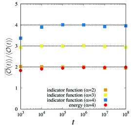
Figure 8: We show the dimensionless ratio $\langle\overline{{\cal O}}\rangle/\langle{\cal O}\rangle$ obtained from numerical simulations versus time. In the long time limit and if the observable is integrable with respect to the infinite density, we have according to Eq. (31) $\langle\overline{{\cal O}}\rangle/\langle{\cal O}\rangle=\alpha$, a behavior we illustrate here for the indicator function, which as mentioned in the text, is an integrable observable for any choice of $\alpha$. The energy observable, is non integrable for $\alpha=4$. Then theory Eq. (76) predicts $\langle\overline{{\cal O}}\rangle/\langle{\cal O}\rangle=1/(1-2/\alpha)=2$, nicely matching the numerics.

We did not present the derivation of Eq. (71) for $0<\gamma<1/3$ since the result is rather intuitive. It means that in this regime the contribution to the kinetic energy comes from the slow atoms where the scaling solution is valid. Technically we consider $\int_{0}^{\infty}v^{2}\rho(v,t){\rm d}v$, and divide the integration into two parts, in the first the density $\rho(v,t)$ in the small $v$ inner region is the scaling solution and in the second the density is approximated by the outer solution, namely the infinite density. Then after integrating over the observable $v^{2}$ we can show that in the long time limit the former is the leading term. For the case $1/3<\gamma<1$ the observable is integrable with respect to the infinite measure and then the opposite situation is found. When $\gamma=1/3$ or $\gamma=1$ one finds logarithmic corrections not treated here.

Using Eq. (19) we find

$$\langle E_{k}(t)\rangle=\langle v^{2}(t)\rangle\sim\underbrace{\int_{0}^{\infty}xe^{-x^{1/\gamma}}\int_{0}^{x}e^{z^{1/\gamma}}{\rm d}z{\rm d}x}_{J_{\gamma}}{\sin(\pi\gamma)\over\Gamma(1+\gamma)\pi\gamma}\left({c\over t}\right)^{2\gamma}\ \ \ \mbox{for}\ \ 0<\gamma<{1\over 3}.$$ (72)

Here the kinetic energy is independent of the specific details of $R(v)$ besides $c$ and $\gamma=1/\alpha$, namely the parameters controlling the behaviour of the rate of escape from the trap at small $v$. This is very different for the case $1/3<\gamma$. Further according to Eq. (72) the velocity PDF $f(v)$ is not at all influencing the long time dynamics of the mean kinetic energy, though we assume that this distribution has finite moments, and support on zero velocity.

The integral $J_{\gamma}$ in Eq. (72), can be evaluated analogously to the calculation of the normalization of $g(x)$ in Eq. (20). The integral converges only for $\gamma<1/3$, and one obtains

$$J_{\gamma}=\frac{\pi\gamma}{\sin(3\pi\gamma)}\frac{\Gamma(1+\gamma)}{\Gamma(1-2\gamma)},$$ (73)

where we can see explicitly the divergence at $\gamma=1/3$ and that $\lim_{\gamma\rightarrow 0}J_{\gamma}\rightarrow 1/3$. Inserting this into (72), we get for the ensemble averaged kinetic energy

$$\left\langle E_{k}(t)\right\rangle\sim\frac{\sin(\pi\gamma)}{\sin(3\pi\gamma)}\frac{1}{\Gamma(1-2\gamma)}c^{2\gamma}t^{-2\gamma}.$$ (74)

From here, we obtain the expectation of the time average immediately

$$\left\langle\overline{E_{k}(t)}\right\rangle\sim\frac{\left\langle E_{k}(t)\right\rangle}{1-2\gamma}\sim\frac{\sin(\pi\gamma)}{\sin(3\pi\gamma)}\frac{1}{\Gamma(2-2\gamma)}c^{2\gamma}t^{-2\gamma}.$$ (75)

Eqs. (74) and (75) confirm that in this phase, in contrast to the phases with $\gamma>1/3$, the average energy is independent of the details of the parent velocity distribution $f(v)$, especially here it is independent of $v_{\max}$.

The asymptotic relations between the ensemble averaged kinetic energy $\left\langle E_{k}(t)\right\rangle$ and its time average $\left\langle\overline{E_{k}(t)}\right\rangle$ in the various phases can therefore be summarized as

$$\boxed{\langle\overline{E}_{k}(t)\rangle\sim\left\{\begin{array}[]{l l}\langle E_{k}\rangle&\ \ 1<\gamma,\\ &\\ {\langle E_{k}(t)\rangle\over\gamma}&\ \ 1/3<\gamma<1,\\ &\\ {\langle E_{k}(t)\rangle\over 1-2\gamma}&\ \ 0<\gamma<1/3.\end{array}\right.}$$ (76)

To obtain the fluctuations of the time averaged energy, namely to calculate the EB parameter Eq. (70) further work is required. We need to evaluate the second moment of the action which in Laplace space is $\langle\hat{{\cal S}}^{2}(p)\rangle={\partial^{2}\hat{P}(u,p)\over\partial u^{2}}|_{u=0}$ and then using Eq. (53)

$$\langle\hat{{\cal S}}^{2}(p)\rangle=\underbrace{{\Phi_{2}^{\prime\prime}(0,p)\over 1-\phi_{2}(0,p)}}_{I_{1}(p)}+\underbrace{{2\Phi_{2}^{\prime}(0,0)\phi_{2}^{\prime}(0,p)\over[1-\phi_{2}(0,p)]^{2}}}_{I_{2}(p)}+\underbrace{{\Phi_{2}(0,p)\phi_{2}^{\prime\prime}(0,p)\over[1-\phi_{2}(0,p)]^{2}}}_{I_{3}(p)}+\underbrace{{2\Phi_{2}(0,p)[\phi_{2}^{\prime}(0,p)]^{2}\over[1-\phi_{2}(0,p)]^{3}}}_{I_{4}(p)}.$$ (77)

Unfortunately all four terms are contributing to the small $p$ limit under investigation. This means that unlike the case $1/3<\gamma$, here the effect of the last interval in the sequence, which we called the backward recurrence time, is dominating the statistics of the time average of the energy. The details of the calculations are presented in the subsection below. We find asymptotically for $0<\gamma<1/3$

$$\boxed{\mbox{EB}={\langle\overline{E_{k}}^{2}(t)\rangle-\langle\overline{E_{k}}(t)\rangle^{2}\over\langle\overline{E_{k}}(t)\rangle^{2}}={\langle{\cal S}^{2}(t)\rangle-\langle{\cal S}(t)\rangle^{2}\over\langle{\cal S}(t)\rangle^{2}}={2\Gamma^{2}(2-2\gamma)\over\Gamma(3-4\gamma)}\left[{\sin^{2}(3\pi\gamma)(1-5\gamma)\over\sin(\pi\gamma)\sin(5\pi\gamma)}+3\gamma\right]-1.}$$ (78)

This expression clearly differs from the EB parameter found in the Darling-Kac phase $1/3<\gamma$, Eq. (70). The latter is universal in the sense that it is valid for any integrable observable. In contrast here the fluctuations are specific to a non-integrable observable, namely the energy provided that $0<\gamma<1/3$. Note that when $\gamma\to 1/3$ from below and above $\mbox{EB}=2\Gamma^{2}(4/3)/\Gamma(5/3)-1\simeq 0.766$, namely Eq. (70) and Eq. (78) match, so the EB parameter is a continuous function of $\gamma$ while its derivative is not. In the range $0<\gamma<1/3$ the EB parameter has a minimum, an effect that we cannot explain intuitively. In Fig. 9 we present numerical results for the EB parameter versus $0<\gamma<1$, comparing it to the analytical theory. A clear transition is observed when the energy observable switches from an integral to a non-integrable observable, a transition found when $\gamma=1/3$.

In the limit $\gamma\to 0$ we find from Eq. (78) $\mbox{EB}=4/5$. To understand this limit we notice that

$$\lim_{\gamma\to 0}\mbox{EB}={\langle(E_{k})^{2}\rangle-\langle E_{k}\rangle^{2}\over\langle E_{k}\rangle^{2}}$$ (79)

where unlike the definition in Eq. (78) here we have the ensemble averaged energy not the time averages. In this limit we have a stagnation effect in the sense that in the measurement time $t$ the system remains in a particular though random velocity state for practically the whole duration of the process namely $\overline{E_{k}}=\int_{0}^{t}E_{k}(t){\rm d}t/t=v^{2}t/t=v^{2}$. Note that we consider here the limit where $t$ is made long and only then $\gamma\to 0$. It is easy to find $\langle E_{k}\rangle=\langle v^{2}\rangle$ and $\langle(E_{k})^{2}\rangle=\langle v^{4}\rangle$ in the limit $\gamma\to 0$ using Eqs. (19, 20). In particular $\exp(-x^{1/\gamma}/c)=1$ if $0<x<1$ otherwise it is zero since $\gamma\to 0$. Hence using Eq. (19) $\langle v^{2}(t)\rangle=\int_{0}^{1}x\int_{0}^{x}{\rm d}z{\rm d}x(c/t)^{2\gamma}=(1/3)(c/t)^{2\gamma}$ and similarly $\langle v^{4}(t)\rangle=(1/5)(c/t)^{4\gamma}$ and indeed $\lim_{\gamma\to 0}\mbox{EB}=[(1/5)-(1/3)^{2}]/(1/3)^{2}=4/5$. To conclude Eq. (78) makes perfect sense in the limit $\gamma\to 0$ marking the stagnation of the dynamics, and $\gamma\to 1/3$ marking the transition to the Darling-Kac phase, in between the solution is not trivial.

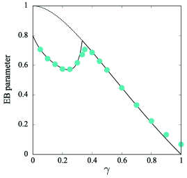
Figure 9: The EB parameter versus $\gamma$ for the kinetic energy observable $v^{2}$. When $\mbox{EB}=0$ we have an ergodic phase found when $\gamma>1$. This ergodicity breaking parameter is a measure for the fluctuations of the time averages and for $1/3<\gamma<1$ is given by Eq. (70). That formula is valid when ever the observable is integrable with respect to the infinite measure. For $0<\gamma<1/3$ the kinetic energy observable is non-integrable, and the system enters a different phase, described by Eq. (78). The dots are obtained from finite time simulations of a model with a parent velocity distribution $f(v)$ which is uniform and the number of particles used was $10^{5}$. The continuous dotted curve is Eq. (70) plotted in the full range $0<\gamma<1$. It holds for example for the indicator function which is an integrable observable in this range, and hence this observable does not exhibit the discontinuous behaviour unlike the energy observable.

VI.1 Formula for $\langle\overline{E}_{k}\rangle$

We now derive Eq. (75) the reader not interested in this technicality may of course skip this sub-section. Specifically we use as a model the uniform velocity PDF $f(v)$ Eq. (36) and the rate function $R(v)$ Eq. (37), though our final results are more general. The main tool is Eq. (55) for $\langle\hat{{\cal S}}(p)\rangle$ which is evaluated in the limit of small $p$, then transformed to $t$, a standard Tauberian procedure valid in the long time limit. From here, as before, we get $\langle\overline{E}_{k}(t)\rangle\sim\langle{\cal S}(t)\rangle/t$.

Eq. (55) is split into two terms

$$\langle{\cal S}(p)\rangle=\hat{H}_{1}(p)+\hat{H}_{2}(p)$$ (80)

with

$$\hat{H}_{1}(p)=-{{\partial\hat{\phi_{2}}(u,p)\over\partial u}|_{u=0}\hat{\Phi}_{2}(0,p)\over\left[1-\hat{\phi}_{2}(0,p)\right]^{2}},\ \ \ \ \ \ \ \hat{H}_{2}(p)=-{{\partial\hat{\Phi}_{2}\left(u,p\right)\over\partial u}|_{u=0}\over 1-\hat{\phi}_{2}(0,p)}.$$ (81)

When $1/3<\gamma$ the derivative $\partial_{u}\hat{\phi}_{2}(u,p)|_{u=0}$ is the mean action increment $\langle s\rangle$ when $p\to 0$. However, here it diverges, since we consider $0<\gamma<1/3$. Recall that $\hat{\Phi}_{2}(u,p)$ is associated with the probability of not jolting namely the term $\hat{H}_{2}(p)$ is stemming from contribution to the total action from the backward recurrence time. In the limit, it was negligible for $1/3<\gamma$ but here both terms are important.

To start we rewrite Eq. (61)

$$\hat{\phi}_{2}(u,p)=1-{1\over v_{{\rm max}}}\int_{0}^{v_{{\rm max}}}\left(1-{R(v)\over p+R(v)+uv^{2}}\right){\rm d}v=1-{1\over v_{{\rm max}}}\int_{0}^{v_{{\rm max}}}{p+uv^{2}\over p+R(v)+uv^{2}}{\rm d}v.$$ (82)

We set $u$ to zero and change variables according to $v^{\alpha}=(pc)^{1/\alpha}z$ and then get

$$\hat{\phi}_{2}(0,p)=1-{(pc)^{1/\alpha}\over v_{{\rm max}}}\int_{0}^{v_{{\rm max}}/(pc)^{1/\alpha}}{{\rm d}z\over 1+z^{\alpha}}.$$ (83)

The upper limit is then taken to be infinity and we find in the small $p$ limit $\hat{\phi}_{2}(0,p)\sim 1-(pc)^{\gamma}\pi\gamma/v_{{\rm max}}\sin\pi\gamma$. The first term here is the normalisation, the second indicates that the mean trapping time is diverging, more precisely this well known Tauberian relation comes from the fat tail of the waiting time PDF Eq. (42). In these calculations and those which now follow we use three integrals

$$\int_{0}^{\infty}{{\rm d}z\over 1+z^{\alpha}}={(\pi/\alpha)\over\sin(\pi/\alpha)},\ \ \ \int_{0}^{\infty}{\alpha z^{\alpha+2}{\rm d}z\over(1+z^{\alpha})^{2}}={(3\pi/\alpha)\over\sin(3\pi/\alpha)},\ \mbox{and}\ \ \ \int_{0}^{\infty}{\alpha^{2}z^{2}{\rm d}z\over(1+z^{\alpha})^{2}}={\pi(\alpha-3)\over\sin(3\pi/\alpha)},$$ (84)

all valid in the regime of interest.

Using the same tricks we find

$$-\partial_{u}\hat{\phi}_{2}(u,p)|_{u=0}\sim\left({c\over v_{{\rm max}}}\right)\left(pc\right)^{3\gamma-1}\int_{0}^{\infty}{z^{\alpha+2}{\rm d}z\over(1+z^{\alpha})^{2}},$$ (85)

and

$$-\partial_{u}\hat{\Phi}_{2}(u,p)|_{u=0}\sim{c^{2}\over v_{{\rm max}}}\left(pc\right)^{3\gamma-2}\int_{0}^{\infty}{z^{2}{\rm d}z\over(1+z^{\alpha})^{2}}.$$ (86)

Inserting Eqs. (85, 87) in Eq. (81) we find the small $p$ limit of $\hat{H}_{1}(p)$ and $\hat{H}_{2}(p)$. It is now easy to transform from $p$ to time $t$ and find

$$\langle\overline{E}_{k}\rangle={\langle{\cal S}(t)\rangle\over t}\sim\left({c\over t}\right)^{2\gamma}\left[\underbrace{{3\gamma\sin(\pi\gamma)\over\Gamma(2-2\gamma)\sin(3\pi\gamma)}}_{H_{1}(t)}+\underbrace{{\sin(\pi\gamma)(1-3\gamma)\over\Gamma(2-2\gamma)\sin(3\pi\gamma)}}_{H_{2}(t)}\right].$$ (87)

The first term vanishes in the limit of $\gamma\to 0$, namely in that limit the time interval $(0,t)$ is effectively collision free, in such a way that the dominating contribution is the backward recurrence time Longest ; Marc (the $H_{2}(t)$ term). This means roughly speaking, that in this limit the backward recurrence time is equal to the measurement time. In contrast when $\gamma\to 1/3$ marking the transition to the integrability of the energy, namely the Darling-Kac phase, the first term which stems from many jumps is diverging. From Eq. (87) we get Eq. (75).

VI.2 EB parameter

To obtain the EB parameter we use Eq. (77) to find the variance of ${\cal S}$ in the long time limit. We consider the four terms $I_{j}(p)$ with $j=1,..,4$ defined in Eq. (77) in the limit $p\to 0$. The calculations are some what similar to those in the previous subsection though now we need to consider second order derivatives with respect to $u$ for example we find

$$\hat{\Phi}_{2}^{\prime\prime}(0,p)\sim{2(pc)^{5/\alpha}\over v_{{\rm max}}p^{3}}\int_{0}^{\infty}{z^{4}{\rm d}z\over(1+z^{\alpha})^{3}}.$$ (88)

and using Eq. (83)

$$I_{1}(p)\sim{2c^{3}(pc)^{4\gamma-3}\int_{0}^{\infty}{z^{4}\over(1+z^{\alpha})^{3}}{\rm d}z\over(\pi\gamma)/\sin(\pi\gamma)}.$$ (89)

Notice that $I_{1}(p)$ is independent of $v_{{\rm max}}$ in this limit, and so are the remaining terms $I_{2}(p),I_{3}(p)$ and $I_{4}(p)$ which are given by

$$I_{2}(p)\sim 2c^{3}(pc)^{4\gamma-3}{\int_{0}^{\infty}{z^{2}\over(1+z^{\alpha})^{2}}{\rm d}z\int_{0}^{\infty}{z^{\alpha+2}\over(1+z^{\alpha})^{2}}{\rm d}z\over[(\pi\gamma)/\sin(\pi\gamma)]^{2}},$$ (90)

$$I_{3}(p)\sim 2c^{3}(pc)^{4\gamma-3}{\int_{0}^{\infty}{z^{\alpha+4}\over(1+z^{\alpha})^{3}}{\rm d}z\over\pi\gamma/\sin\pi\gamma},$$ (91)

and similarly

$$I_{4}(p)\sim 2c^{3}(pc)^{4\gamma-3}{\left[\int_{0}^{\infty}{z^{\alpha+2}\over(1+z^{\alpha})^{2}}{\rm d}z\right]^{2}\over\left[\pi\gamma/\sin\pi\gamma\right]^{2}}.$$ (92)

Inverting to the time domain we see that $\langle S^{2}(t)\rangle\propto t^{2-4\gamma}$. The integrals in Eqs. (89 -92) are tabulated in Mathematica, so summing all the four terms in Eq. (77) and using $\langle S(t)\rangle$, Eq. (87), we obtain the variance $\langle S^{2}(t)\rangle-\langle S(t)\rangle^{2}$ and this after normalization yields the EB parameter Eq. (78).

VII Distribution of time averages in the non-integrable phase

We will now obtain the PDF of the random variable $\Upsilon={\cal S}(t)/\langle{\cal S}(t)\rangle={\overline{E}}_{k}(t)/\langle\overline{E}_{k}(t)\rangle$, namely the normalised time averaged kinetic energy, in the phase when this observable is non-integrable with respect to the infinite density. Recall, that when the energy is integrable, we obtain the universal Mittag-Laffler law Eq. (69). Unlike the latter case, the PDF of $\Upsilon$ denoted $P_{\alpha}(\Upsilon)$ will now depend on the microscopical details of the model, in particular the PDF of the speed after collisions $f(v)$. Here we find $P_{\alpha}(\Upsilon)$ for the model under study, namely the case where $f(v)$ is uniform. The analysis does not allow us to obtain a general solution for $P_{\alpha}(\Upsilon)$ for all $3<\alpha$ and we mainly revert to approximations. This is unlike the variance, given in terms of the EB parameter, Eq. (78) which was calculated exactly. Since the calculations are lengthy, here we provide the outline of the theory, focusing on three cases, $\alpha=4$, $\alpha=6$ and $\alpha\to\infty$. Comparing the semi-analytical solution to simulations we gain insight on a new type of transition, which shows up as a sudden blow up of $P_{\alpha}(\Upsilon)$ for $\Upsilon\to 0$. The effect is certainly not found for the Mittag-Leffler distribution, within the integrable phase $\alpha<3$.

The double Laplace transform of the action propagator $P(S,t)$ is given by $\widehat{P}(u,p)$ and the Montroll-Weiss type equation Eq. (53). The technical problem is to invert this solution in the limit of long times corresponding to the Laplace variable $p\to 0$ being small. The functions $P({\cal S},t)$ and $\widehat{P}(u,p)$ attain scaling forms, denoted $P({\cal S},t)\sim t^{1-\alpha/2}f_{\alpha}({\cal S}/t^{1-2/\alpha})$ and $P(u,p)\sim(1/p)g_{\alpha}(u/p^{1-2/\alpha})$. Here the limit under study is $t\to\infty$ and ${\cal S}\to\infty$ the ratio ${\cal S}/t^{1-2/\alpha}$ remaining fixed and similarly in Laplace space. Note that we showed in Eq. (87) that $\langle{\cal S}(t)\rangle\propto t^{1-2/\alpha}$, hence the scaling of ${\cal S}$ with time we use here is consistent with that observation. The two scaling solutions are related by the laws of Laplace transform

$$\frac{1}{p}g_{\alpha}(\frac{u}{p^{1-2/\alpha}})=\int\limits_{0}^{\infty}d{\cal S}\int\limits_{0}^{\infty}dt\;e^{-u{\cal S}}e^{-pt}\frac{1}{t^{1-2/\alpha}}f_{\alpha}(\frac{{\cal S}}{t^{1-2/\alpha}}).$$ (93)

Substituting $x=\frac{{\cal S}}{t^{1-2/\alpha}}$ and setting $p=1$ turns Eq. (93) into the integral equation

$$g_{\alpha}(y)=\int\limits_{0}^{\infty}dx\;K_{\alpha}(yx)f_{\alpha}(x)$$ (94)

relating $g_{\alpha}(y)$ and $f_{\alpha}(x)$ via this convolution transform with kernel

$$K_{\alpha}(x)=\int\limits_{0}^{\infty}dt\;e^{-xt^{1-2/\alpha}}e^{-t}.$$ (95)

For the scaling function $g_{\alpha}(y)$, with $\alpha>3$, i.e. in the non-Darling-Kac phase, we obtain from the $p\rightarrow 0$ limit of $\widehat{P}(u,p)$ Eq. (53) the following exact form

$$g_{\alpha}(y)=\frac{\int\limits_{0}^{\infty}\frac{1}{1+yz^{2}+z^{\alpha}}dz}{\int\limits_{0}^{\infty}\frac{1+yz^{2}}{1+yz^{2}+z^{\alpha}}dz}.$$ (96)

The goal is to obtain from this by inversion of Eq. (94) the scaling function $f_{\alpha}(x)$, which is a rescaled version of the limiting probability density $P_{\alpha}(\Upsilon)$ of the normalized time average $\Upsilon$. Such an inversion can be achieved in principle by a Mellin transform of both sides of Eq. (94) resulting in [Polyanin , p.997]

$$\widetilde{g}_{\alpha}(s)=\widetilde{K_{\alpha}}(s)\widetilde{f}_{\alpha}(1-s),$$ (97)

where $\widetilde{g}_{\alpha}(s)=M[g_{\alpha}(y);s]=\int\limits_{0}^{\infty}dy\;g_{\alpha}(y)y^{s-1}$ is the Mellin transform of $g_{\alpha}(y)$, and $\widetilde{K_{\alpha}}(s)$ and $\widetilde{f}_{\alpha}(s)$ is defined analogously. Solving Eq. (97) for $\widetilde{f}_{\alpha}(s)$ and applying the inverse Mellin transformation gives

$$f_{\alpha}(x)=M^{-1}[\widetilde{f}_{\alpha}(s);x]=M^{-1}[\frac{\widetilde{g}_{\alpha}(1-s)}{\widetilde{K}_{\alpha}(1-s)};x],$$ (98)

and finally by rescaling the desired limit density is obtained as

$$P_{\alpha}(\Upsilon)=C_{\alpha}f_{\alpha}(x)|_{x=C_{\alpha}\Upsilon},$$ (99)

where $C_{\alpha}=\left\langle x\right\rangle_{f_{\alpha}}=\int\limits_{0}^{\infty}dx\;xf_{\alpha}(x)$. The rescaling implies that the mean is $\left\langle\Upsilon\right\rangle_{P_{\alpha}}=\int\limits_{0}^{\infty}d\Upsilon\;\Upsilon P_{\alpha}(\Upsilon)=1$, as requested. While in principle along these steps the problem of calculating the limit distribution $P_{\alpha}(\Upsilon)$ is solved, a fully analytic solution is available only in two cases, $\alpha=4$ and $\alpha=\infty$. For $\alpha=4$ the integrals in Eq. (96) can be evaluated by residue calculus yielding after some calculations the simple result

$$g_{4}(y)=\frac{1}{1+y},$$ (100)

with Mellin transform $\widetilde{g}_{4}(s)=\Gamma(s)\Gamma(1-s)$. Since the Mellin transform $\widetilde{K_{\alpha}}(s)$ of the integral kernel is also known in full generality, $\widetilde{K}_{\alpha}(s)=\Gamma(s)\Gamma(1-(1-2/\alpha)s)$, we get the quotient in Eq. (98), and in addition we can invert from Mellin space to obtain $f_{4}(x)=\frac{1}{\sqrt{\pi}}e^{-\frac{x^{2}}{4}}$. The scaling factor $C_{4}=\left\langle x\right\rangle_{f_{4}}$ follows from the general relation between the $n$-th derivative $g_{\alpha}^{(n)}(y=0)$ and the moments $\left\langle x^{n}\right\rangle_{f_{\alpha}}$ of $f_{\alpha}(x)$

$$g_{\alpha}^{(n)}(0)=K_{\alpha}^{(n)}(0)\left\langle x^{n}\right\rangle_{f_{\alpha}}=(-1)^{n}\Gamma(1+n(1-\frac{2}{\alpha}))\left\langle x^{n}\right\rangle_{f_{\alpha}},$$ (101)

which follows directly from Eq. (94). For $\alpha=4$ we get $C_{4}=\left\langle x\right\rangle_{f_{4}}=\frac{2}{\sqrt{\pi}}$, so that we obtain for $P_{4}(\Upsilon)$ according to Eq. (99) a half Gaussian distribution

$$P_{4}(\Upsilon)=\frac{2}{\pi}e^{-\frac{\Upsilon^{2}}{\pi}}$$ (102)

as an exact result. It is merely a coincidence, that this half Gaussian is found also in the Mittag-Leffler phase, when $\alpha=2$, see Fig. 6. We can proceed similarly for $\alpha\rightarrow\infty$, because all integrals and Mellin transforms are known exactly also in this case yielding

$$g_{\infty}(y)=\frac{1}{\sqrt{y}}\arctan\sqrt{y}$$ (103)

and eventually

$$P_{\infty}(\Upsilon)=\frac{1}{2\sqrt{3}}\frac{1}{\sqrt{\Upsilon}}\theta(3-\Upsilon),$$ (104)

where we use the step function. This result diverges at the origin $\Upsilon\to 0$, and we will soon show that this is valid for any $\alpha>4$. Note that PDF is cutoff sharply at $\Upsilon=3$ an effect which is related to the underlying uniform distribution of $v$, Eq. (36). More precisely, we may explain this result, by noting that the atom maintains a constant velocity for practically all the duration of the experiment, since $\alpha\to\infty$ or $\gamma=1/\alpha\to 0$. Then $\Upsilon=v^{2}/\langle v^{2}\rangle$ and using the uniform PDF of velocities Eq. (36) we get Eq. (104). In Fig. 10 we present simulation results for $\alpha=50$ and compare them to theory $\alpha\to\infty$. These match well with the limiting PDF $P_{\infty}(\Upsilon)$, the exception is that the histogram is smeared and does not show the step like structure of limiting PDF which is found at $\Upsilon=3$.

Figure 10: Histogram of the normalized time averaged energy $P_{\alpha}(\Upsilon)$, obtained from numerical simulations with $\alpha=50$ is compared with the limiting PDF Eq. (104). In the limit the PDF is sharply cutoff at $\Upsilon=3$ an effect which is smeared out with the finite time, finite $\alpha$ simulations.

For the experimentally also relevant case $\alpha=6$ we can still get from Eq. (96) by residue calculus a fully analytic expression for $g_{6}(y)$, but the result is very lengthy involving 3rd roots etc., and it does not simplify as in the case $\alpha=4$. Therefore one cannot analytically calculate its Mellin transform. This led us to find an approximate scaling function $g_{6}^{\approx}(y)$, which deviates only little from the true function $g_{6}(y)$, but for which the Mellin transform is known analytically. The general ideas is to match in $g_{6}^{\approx}(y)$ the true small $y$-behavior and the large $y$-asymptotics of $g_{6}(y)$, which we know analytically from an analysis of Eq. (96). The simple form

$$g_{6}^{\approx}(y)=(1+\frac{2}{3}y)^{-\frac{3}{4}}$$ (105)

shares with the exact function $g_{6}(y)$ the identical first and second derivative at $y=0$, and the exponent of the asymptotic behavior for $y\rightarrow\infty$. The relative deviation of $g_{6}^{\approx}(y)$ from $g_{6}(y)$ is strictly less than 4.2%. This function $g_{6}^{\approx}(y)$ can be Mellin transformed Prudnikov , and leads via Eq. (98) and subsequent rescaling to an analytical expression for $P_{6}^{\approx}(\Upsilon)$, which can be expressed in terms of a Fox-H function Fox as

$$P_{6}^{\approx}(\Upsilon)=\frac{3}{4\Gamma(\frac{5}{3})\Gamma(\frac{3}{4})}H_{1,1}^{1,0}\left(\frac{3}{4\Gamma(\frac{5}{3})}\Upsilon\left|\begin{array}[]{c}(\frac{1}{3},\frac{2}{3})\\ (-\frac{1}{4},1)\end{array}\right.\right).$$ (106)

As mentioned, after rewriting this expression in terms of a Meijer G-function [Prudnikov , p.629], we can plot the result with Mathematica, see Fig. 11.

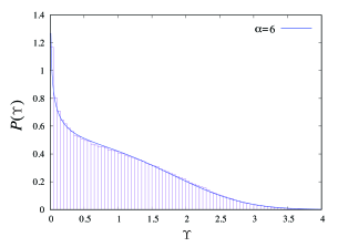
Figure 11: Simulations and theory Eq. (106) for the distribution of the time averaged energy $P_{\alpha}(\Upsilon)$, for $\alpha=6$. Here the observable is non-integrable with respect to the infinite density, and $P_{6}(\Upsilon)$ diverges at $\Upsilon\to 0$, indicating very long sticking times close to zero speed, for some of the atoms which have very low energy compared to the mean.

VII.1 Accumulation effect for $\alpha>4$

We mentioned already that $P_{\alpha}(\Upsilon)$ diverges at the origin $\Upsilon\to 0$ for any $\alpha>4$ and explained that this means that a large population of particles remain slow for the whole duration of the experiment. Now we wish to characterise this effect more precisely.

It is easy to see that the exact asymptotic behavior of $g_{\alpha}(y)$ for $y\rightarrow\infty$ is given by

$$g_{\alpha}(y)\sim ry^{-\eta},$$ (107)

with decay exponent

$$\eta=\eta(\alpha)=\frac{\alpha}{2(\alpha-2)}$$ (108)

and decay amplitude

$$r=r(\alpha)=\frac{\alpha-2}{2}\sin\frac{\pi}{\alpha-2}.$$ (109)

From that the small $x$-asymptotics of $f_{\alpha}(x)$ follows exactly as

$$f_{\alpha}(x)\sim t(\alpha)x^{-s_{0}(\alpha)}$$ (110)

with exponent

$$s_{0}(\alpha)=1-\eta(\alpha)=1-\frac{\text{ }\alpha}{2(\alpha-2)}=\frac{\alpha-4}{2\alpha-4},$$ (111)

and amplitude

$$t(\alpha)=\frac{r(\alpha)}{\sqrt{\pi}\Gamma(\eta(\alpha))}=\frac{\frac{\alpha-2}{2}\sin\frac{\pi}{\alpha-2}}{\sqrt{\pi}\Gamma(\frac{\alpha}{2(\alpha-2)})}.$$ (112)

The following table gives an overview for the resulting behavior of $f_{\alpha}(x\rightarrow 0)\sim$ $t(\alpha)x^{-s_{0}(\alpha)}$ and of the limit distribution $\rho_{\alpha}^{\ast}(x\rightarrow 0)=C_{\alpha}f_{\alpha}(C_{\alpha}x\rightarrow 0)$. With the explicit form of $C_{\alpha}$ derivable from the exact form of $g_{\alpha}^{\prime}(0)$

$$C_{\alpha}=\left\langle x\right\rangle_{f_{\alpha}}=\frac{\sin(\pi/\alpha)}{\sin(3\pi/\alpha)}\frac{1}{\Gamma(2-\frac{2}{\alpha})}=\frac{1}{1+2\cos\frac{2\pi}{\alpha}}\frac{1}{\Gamma(2-\frac{2}{\alpha})}$$ (113)

this yields

$$\begin{array}[]{ccc}\alpha&f_{\alpha}(x\rightarrow 0)&P_{\alpha}(x\rightarrow 0)\\ \alpha\rightarrow\infty&\frac{1}{2}x^{-\frac{1}{2}}&\frac{1}{2\sqrt{3}}x^{-\frac{1}{2}}\\ \alpha=50&\frac{24\sin(\frac{\pi}{48})}{\sqrt{\pi}\Gamma(\frac{25}{48})}x^{-\frac{23}{48}}&\frac{24\sin(\frac{\pi}{48})}{\sqrt{\pi}\Gamma(\frac{25}{48})[(1+2\cos(\frac{\pi}{25}))\Gamma(\frac{49}{25})]^{\frac{25}{48}}}x^{-\frac{23}{48}}\\ \alpha=6&\frac{\sqrt{2}}{\sqrt{\pi}\Gamma(\frac{3}{4})}x^{-\frac{1}{4}}&\frac{1}{2^{\frac{1}{4}}\sqrt{\pi}\Gamma(\frac{3}{4})\Gamma(\frac{5}{3})^{\frac{3}{4}}}x^{-\frac{1}{4}}\\ \alpha=5&\frac{3\sqrt{3}}{4\sqrt{\pi}\Gamma(\frac{5}{6})}x^{-\frac{1}{6}}&\frac{3\sqrt{3}[\frac{1}{2}(3-\sqrt{5})]^{\frac{5}{12}}}{4\sqrt{\pi}\Gamma(\frac{5}{6})\Gamma(\frac{8}{5})^{\frac{5}{6}}}x^{-\frac{1}{6}}\\ \alpha=4&\frac{1}{\sqrt{\pi}}x^{0}&\frac{2}{\pi}x^{0}\\ \alpha=\frac{7}{2}&\frac{3\sqrt{3}}{8\sqrt{\pi}\Gamma(\frac{7}{6})}x^{\frac{1}{6}}&\frac{3\sqrt{3}}{8\sqrt{\pi}\Gamma(\frac{7}{6})}\left[\frac{\cos(\frac{3\pi}{14})}{\sin(\frac{\pi}{7})\Gamma(\frac{10}{7})}\right]^{\frac{7}{6}}x^{\frac{1}{6}}\\ \alpha=\frac{10}{3}&\frac{\sqrt{2}}{3\sqrt{\pi}\Gamma(\frac{5}{4})}x^{\frac{1}{4}}&\frac{(1+\sqrt{5})^{\frac{5}{2}}}{12\sqrt{\pi}\Gamma(\frac{5}{4})\Gamma(\frac{7}{5})^{\frac{5}{4}}}x^{\frac{1}{4}}\\ \begin{array}[]{c}\alpha=3+\varepsilon,\\ \varepsilon\rightarrow 0\end{array}&\varepsilon x^{\frac{1}{2}-\varepsilon}&(\frac{2\sqrt{3}}{\pi\Gamma(\frac{7}{5})})^{\frac{3}{2}}\varepsilon^{-\frac{1}{2}}x^{\frac{1}{2}-\varepsilon}.\end{array}$$ (114)

This array of equations shows that $\alpha=4$ takes a special role as it separates diverging behavior of $f_{\alpha}(x)$ near $x=0$ for $\alpha>4$ from vanishing behavior for $3<\alpha<4$. Note also the diverging amplitude in $\rho_{3+\varepsilon}^{\ast}(x)$ as $\varepsilon\rightarrow 0$ in contrast to the vanishing amplitude of $f_{3+\varepsilon}(x)$, which is a consequence of the diverging scaling factor $C_{3+\varepsilon}\sim\varepsilon^{-1}$.

VII.2 Physical consequences

We discovered for $\alpha>4$, an accumulation effect, namely the divergence of the PDF of the time averages, found at low energies e.g. where $\alpha=6$ and $\Upsilon\to 0$. This means that a significant population of atoms remains at small speeds for the whole duration of the experiment. In turn, this is useful when one wishes to reduce scattering or spatial spreading, namely holding atoms close to the dark zero momentum state for long durations. Thus, while for the optimization of the commonly used relaxation time of the full width at half maximum (FWHM) of the velocity packet, which decays as $t^{-1/\alpha}$, one should consider small values of $\alpha$ to obtain fast relaxation (say $\alpha=2$), to maintain some of the population with small kinetic energy for long durations, large values of $\alpha$ (say $\alpha=6)$ are beneficial, as the trapping times become statistically longer. Surprisingly, $\alpha=4$ marks a quantitative transition of the low energy statistics, which we discovered from the analysis of the time averages.

VIII Perspective

The rate of escape from the velocity trap, $R(v)\propto v^{\alpha}$ for small $v$, implies that for laser cooled systems the mean escape time is infinite when $1<\alpha$ or equivalently $\gamma<1$. From the point of view of cooling this is an advantage, in the sense that typical speeds are low (nano-Kelvin regime). At the same time this leads to the applicability of infinite ergodic theory, including the non-normalisable measure. The system shares some features which are similar to glassy dynamics, in particular the trap model WEB . In that model, we have a density of states $\rho(E)=\exp[-E/T_{g}]/T_{g}$ where $E>0$ are the trap depths and $T_{g}$ a measure of disorder. The system is in contact with a heat bath at temperature $T$. We will not go into the details of the anomalous dynamics in this model, however we point out that also here we encounter a non-normalisable state. The partition function is $Z=\int_{0}^{\infty}\rho(E)\exp(E/T){\rm d}E$ (here $k_{B}=1)$ and hence it diverges when $T_{g}>T$. This low temperature glassy phase also corresponds to the case where the mean trapping time diverges and where one finds anomalous kinetics. Thus, for both the sub-recoiled system and the trap model, we find diverging mean trapping times and also the blow up of the normalisation of the usual steady state. Bouchaud described such systems as exhibiting weak ergodicity breaking, since one has exploration of phase space although time and ensemble averages differ WEB . Mathematicians, use the term infinite ergodic theory, since they realise that the non-normalisable measure is the key ingredient of the theory. Further, this non-normalisable state is related to the normalised distribution $\rho(v,t)$ see Eq. (24), and it is approached from a broad class of initial conditions. Thus, some actually call the dynamics ergodic, i.e. the term infinite ergodic theory implies the dynamics is ergodic, while in the physics literature others describe it as non-ergodic. In short one should distinguish between the operational definition of ergodicity, time and ensemble averages coincide, and the fact that in the long-time limit a unique density is approached, be it normalised or not. We conclude that weak ergodicity breaking and infinite ergodic theory are deeply related. The statistical theory applies both, to models in a non-equilibrium setting like laser cooled atoms, but also to systems with a canonical Boltzmann-Gibbs measure even if the latter is not normalised Erez .

What are the consequences for laser cooling? Remarkably, using Eq. (71) we conclude that the most efficient cooling, in the sense of the fastest relaxation of the mean energy, is found for $\gamma=1/3$. Thus the transition in the ergodic properties of the system investigated here, which takes place when $\alpha=3$ or $\gamma=1/3$, is physically connected to the optimal cooling of energy. This is not a coincidence, namely at the transition point the time dependence changes, though the fact that this point is optimal seems to us as merely good luck. In contrast, for the FWHM of the velocity packet Reichel , we do not have such an optimum. Instead, as mentioned, it decays like $t^{-1/\alpha}$ favouring small values of $\alpha$ for faster relaxation Reichel . Thus the classification of an observable as either integrable (energy, $\gamma>1/3$) or non-integrable (energy $\gamma<1/3$, FWHM) with respect to the infinite invariant measure is crucial, both mathematically and physically. We should note that the FWHM is not a dynamical observable, in the sense that it cannot be obtained as a functional of a single particle path.

In the context of sub-recoil laser cooling our work raised a few questions and here we point out possible extensions.

• It is a challenge to see if quantum Monte Carlo simulations CT can be used to investigate numerically the non-normalisable state and the time and ensemble averages.

• Experimentally finding the infinite density is another obvious challenge. Single atom experiments yield direct insights on the trajectories and the time averages Katori ; Stroescu ; Hohmann ; Widera .

• In our examples we used simple forms for $f(v)$ and $R(v)$. It is important to realise that our main results are generally valid, like the applicability of infinite ergodic theory, though it is clear that details do depend on the microscopical behaviour of these functions. In this context we have recently considered preparation other models, including the case where the process is not renewed after each jolt. The main results are left unchanged.

• What happens to such a gas of atoms in the presence of some binding field, e.g. a harmonic trap? What is the pressure of the gas? What will happen when we add interactions? Will that drive the system to a true thermal state?

• When we considered time averages, the measurement starts when the process is initiated (lower limit of the time integral is zero). Instead one may prepare the system at time $t=0$, then wait until a time $t_{a}$ and only then perform a measurement, i.e. time average in the interval $(t_{a},t_{a}+t)$. In this case we expect that statistical properties of the system will depend on the ageing time $t_{a}$. One can then wonder whether the infinite measure will play an important role also under these conditions? In this regard we may be optimistic, see the modification of Darling-Kac theorem to the ageing regime, in the context of deterministic dynamics Akimoto .

• Sisyphus cooling is also described in terms of Lévy processes Castin ; Zoller ; RenzoniT ; Sagi ; Kessler1 ; Dechant ; AghionPRX and infinite covariant densities were studied in this context Kessler ; Holz . Hence the statistical framework of non-normalised states is indeed widely applicable Renzoni . However for Sisyphus cooling the physics is orthogonal to the current one. The Sisyphus friction force is vanishing for large $v$, and thus the non-normalisable trait comes from the high speed particles Kessler . Here, we have the opposite situation, the rate is anomalous for small $v$. Technically this is related to the fact that for optical lattices infinite covariant densities are studied, while here the focus on infinite invariant densities.

• According to the model, the width of the velocity distribution shrinks with time. And as mentioned in the text, this was indeed observed in experiments till times of order milliseconds. Setting aside experiments, in the limit of $t\to\infty$ the model’s predicts a complete pile up at zero velocity, which seems to be a far fetched idea. We have thus considered an idealised situation, in fact, one could introduce some cutoffs to the process using $R(v)\propto v^{\alpha}+\epsilon$ where $\epsilon$ is very small. Such a cutoff could be important as it would mean that in the very long time limit the system will eventually relax to a normalised state. Indeed, in the absence of cutoffs the time renewal process is scale free and hence it is a random fractal. Like any fractal in nature, cutoffs could be important, as is well known.

• As shown here clearly, and as well known more generally, the theory of infinite ergodic theory is a theory of observables. For example, in our study the indicator function $I(v_{a}<v(t)<v_{b})$ is integrable with respect to the infinite density when $0<v_{a}$ and non-integrable if $v_{a}=0$. This is because of the non-integrable nature of the infinite density at small $v$, which, as stressed, is related to the fact that $R(v)\sim v^{\alpha}$. The kinetic energy is integrable when $1/3<\gamma=1/\alpha<1$, and this has consequences for the ergodic properties of the process. One could consider other observables like $|v|$, the main conclusions of this paper would be left unchanged. It should be noted that also when the invariant measure is finite, and a usual steady state exists an observable can be non-integrable, e.g. in a thermal setting a particle in a harmonic trap, has a Boltzmann density proportional to $\exp(-kx^{2}/2k_{B}T)$, hence an observable which might seem a bit weird to some, like ${\cal O}(x)=\exp(x^{4})$ is non-integrable. The case of non-integrable observables with respect to the steady state, i.e. $\alpha<1$, is of some theoretical interest in the context of the stochastic model under study. At first this might seem academic since so far in experiment $\alpha>1$, however this could be of interest in dimensions greater that unity, see below. An issue in our mind is, whether a specific observable is physically interesting or measurable, and we worked under the assumption that energy is a physically worthy observable.

• We considered here the parent velocity distribution $f(v)$ being a constant at small $v$, e.g. a uniform velocity distribution. In Bertin it was suggested that $f(v)=\mbox{const}\ v^{d-1}$ for $v<v_{{\rm max}}$ and $d$ is the dimension. Hence as mentioned the focus of this paper was on one dimensional systems, mainly for the sake of simplicity Nir . However, once again the main conclusions of our paper are left unchanged, or more correctly, when minor adaptations are made, we may reach similar conclusions. For example, the infinite density in the general case, ${\cal I}_{v}(v)\propto v^{-\alpha+d-1}$, which is clearly non-normalisable when $\alpha-d+1>1$. Hence the case $\alpha=2$ and $d=2$ is special, as it falls on the border between ergodicity in its usual sense and infinite ergodic theory. Such cases are left for future work.

IX Summary

Our starting point was the master equation for the speed of the particle which was previously studied with several methods CT ; Bertin . Here we highlighted the infinite measure ${\cal I}_{v}(v)$ which is a non-normalisable quasi-steady state of the system. To explore the ergodic properties of the system we introduced a generalised Lévy walk approach. This tool gives a Montroll-Weiss like formula, Eq. (53), which is a formal solution to the problem, but more importantly, it can be analysed in the long-time limit giving statistical information on the distribution of the action ${\cal S}(t)$ and from it the distribution of the time average of the energy $\overline{E_{K}}(t)={\cal S}(t)/t$. Here we used the fact that between collision events the momentum is conserved, so the speed is constant changing abruptly at random times. With this method we are able to obtain the properties of the time averages which are functionals of the stochastic process. We focused on the kinetic energy of the particles, however, the approach presented here, is more general. Technically the increments of the walk are action increments $s$, and the joint PDF of the increments $s$ and the waiting times, are the basic ingredients of this coupled walk.

We find three phases in the ergodic properties of the process. The case $\gamma>1$, corresponding to a finite mean time between collisions, was not considered here in detail, since the standard ergodic theory holds as the invariant measure is normalisable. In the regime $1/3<\gamma<1$ the Darling-Kac theorem holds, for the observable of interest. This means that we may quantify the fluctuation of the time averages using the Mittag-Leffler law, Eq. (68), which is a universal type of statistical law in these type of problems. More precisely this theorem is valid for observables which are integrable with respect to the infinite density. Finally, when $0<\gamma<1/3$, the energy observable is non-integrable with respect to the infinite density. Here the mean action increment $\langle s\rangle$ diverges together with the mean time between collisions. The consequence of these phases manifest themselves in several predictions. The decay with time of the ensemble energy, Eq. (71), goes through a qualitative change at the boundary between integrability and non-integrability $\gamma=1/3$. Similarly, for the relation between the mean of the time average and the ensemble average, Eq. (76). Finally, the EB parameter, Eq. (70) and Eq. (78), characterises the fluctuations of the time average and it too exhibits a discontinuous behaviour at $\gamma=1/3$. Thus we have exposed the rich consequences of the fact that an observable is tuned from being integrable to non-integrable. Interestingly, experiments use $\alpha=4$ (where energy is non-integrable) and $\alpha=2$ (where energy is integrable), so we believe that the classification we performed is of possible practical value. Finally, we discovered in Sec. VII another sort of transition. For $\gamma<1/4$ the PDF $P(\Upsilon)$ exhibits an accumulation effect, blowing up at $\Upsilon\to 0$, see Fig. 11. This implies that some of the particles remain in the very cold phase, in the sense of very small velocities, for very long periods.

Acknowledgements The support of Israel Science Foundation’s grant 1614/21 is acknowledged (EB). This work was supported by the JSPS KAKENHI Grant No 240 18K03468 (TA). We thank Tony Albers, Nir Davidson and Lev Khaykovich for helpful suggestions.

X Appendix A

We analyse, laser cooled atoms following the method of Bertin and Bardou Bertin . One idea is to analyse the dynamics of the lifetime $\tau(v)$, taken as a state variable instead of the velocity as done in the main text. As mentioned in the main text, the process in the time interval $(0,t)$ is characterised by a set of uncorrelated speeds $(v_{1},....v_{N})$ all drawn from the common PDF $f(v)$. Here $N(t)$ is the random number of velocity updates (collision events) in the time interval $(0,t)$. These velocity updates are taking place at random times $(t_{0},t_{1},...t_{N-1})$, and $t_{0}=0$ is the origin of time. The waiting times $\tilde{\tau}_{i}=t_{i}-t_{i-1}$ are drawn from an exponential PDF $q(\tilde{\tau}|v)$, Eq. (1), defined by the lifetime $\tau(v_{i})$. The lifetimes are thus fluctuating: every update of the velocity implies a modification of the lifetime. We have the sequence of lifetimes $(\tau_{1}(v_{1}),\tau_{2}(v_{2}),\cdots)$ and this is a useful characteristic of the process. Given the dependence of the lifetime on $v$, namely given the function $\tau(v)$, then, if we find the PDF of the lifetime at time $t$, we can predict the velocity PDF.

The bare PDF of the lifetimes is given by the chain rule $\psi(\tau)=f(v)|{\rm d}v/{\rm d}\tau|$. More precisely this is the PDF of the lifetime, immediately after a collision event. It, of course, differs from the PDF of the lifetime at time $t$, which is denoted $P(\tau,t)$. At time $t$, it is more likely to find an atom with a long lifetime compared with a short one (if you arrive at a bus station randomly, you are more likely to fall on a long time interval between bus arrivals, if compared to short ones). For $\tau(v)\propto v^{-\alpha}$ for $v\to 0$ the chain rule gives

$$\psi(\tau)\propto\tau^{-1-\gamma},\ \mbox{and}\ \gamma=1/\alpha$$

As mentioned, we assume $f(0)\neq 0$, namely we assume that a particle can be injected at small speed values. If $\alpha>1$ we have a diverging mean lifetime. Of course, the PDF of lifetimes $\psi(\tau)$ is not the same as the PDF of the waiting times $\phi_{1}(\tilde{\tau})$ discussed in the main text, though both share the same type of power law decay.

The master equation for the lifetime PDF is

$${\partial P\over\partial t}=-{P\over\tau}+\psi(\tau)\int_{0}^{\infty}{P(\tau^{\prime},t)\over\tau^{\prime}}{\rm d}\tau^{\prime}.$$ (115)

Here both in the loss and the gain terms $1/\tau$ is the rate of leaving state $\tau$. In this equation $f(v)$ appears indirectly through $\psi(\tau)$. In equilibrium, namely $\gamma>1$ we have

$$\lim_{t\to\infty}P(\tau,t)={\tau\psi(\tau)\over\langle\tau\rangle},$$ (116)

where the mean is $\langle\tau\rangle=\int_{0}^{\infty}\tau\psi(\tau){\rm d}\tau$. The fact that we multiply $\psi(\tau)$ with $\tau$ means that in equilibrium we favour the sampling of larger lifetimes, compared to those distributed with the bare PDF $\psi(\tau)$. When $\gamma<1$ the normalisation $\langle\tau\rangle$ diverges. Instead we replace the mean with an effective average $\langle\tau\rangle_{\rm eff}=\int^{t}\tau\psi(\tau){\rm d}\tau\propto t^{1-\gamma}$. Then inspired by Eq. (116) we expect

$$P(\tau,t)\sim b_{1}{\tau\psi(\tau)\over t^{1-\gamma}},$$ (117)

where $b_{1}$ needs a calculation. Already from these arguments we expect to find an infinite density for the lifetimes

$$\lim_{t\to\infty}t^{1-\gamma}P(\tau,t)=b_{1}\tau\psi(\tau)={\cal I}_{\tau}(\tau).$$ (118)

Here the area under the function ${\cal I}_{\tau}(\tau)$ clearly diverges since the mean lifetime is infinite. From here we may find the infinite density of the velocity, using the chain rule. Namely $\rho(v,t)=P(\tau,t)|{\rm d}\tau(v)/{\rm d}v|$ and then using Eq. (118) we get Eq. (24) (besides a prefactor which we still need to obtain). Note that the infinite densities ${\cal I}_{\tau}(\tau)$ or ${\cal I}_{v}(v)$ are non-normalised due to their large or small argument behaviour respectively.

To solve Eq. (115) we introduce the Laplace transform

$$\hat{P}(\tau,p)=\int_{0}^{\infty}e^{-pt}P(\tau,t){\rm d}t$$ (119)

where we use the convention that the argument in the parentheses, i.e. $p$ or $t$, defines the space we are working in. Using the initial condition, we have $P(\tau,t)=\psi(\tau)$ at time $t=0$ and hence the Laplace transform of Eq. (115) gives

$$p\hat{P}(\tau,p)-\psi(\tau)=-{\hat{P}(\tau,p)\over\tau}+\psi(\tau)\int_{0}^{\infty}{\rm d}\tau^{\prime}{\hat{P}(\tau^{\prime},p)\over\tau^{\prime}}.$$ (120)

Using the normalisation condition $\int_{0}^{\infty}\hat{P}(\tau,p){\rm\tau}=1/p$ after some straight-forward rearrangement we find

$$K(\tau,p)=\psi(\tau)\int_{0}^{\infty}K(\tau^{\prime},p){\rm d}\tau^{\prime},$$ (121)

where $K(\tau,p)=\hat{P}(\tau,p)(p+1/\tau)$. From Eq. (121) we have $K(\tau,p)=\psi(\tau)h(p)$, where we use the fact that $\psi(\tau)$ is normalised. Hence we get

$$\hat{P}(\tau,p)={\psi(\tau)\over p+1/\tau}h(p),$$ (122)

To determine $h(p)$ we use normalisation $\int_{0}^{\infty}\hat{P}(\tau,p){\rm d}\tau=1/p$. We thus recover the exact result in Bertin

$$\hat{P}(\tau,p)={1\over p\tau^{*}(p)}{\tau\psi(\tau)\over 1+p\tau}\ \ \mbox{with}\ \ \ \tau^{*}(p)=\int_{0}^{\infty}{\tau^{\prime}\psi(\tau^{\prime}){\rm d}\tau^{\prime}\over 1+p\tau^{\prime}}.$$ (123)

We analyse two cases. The first corresponds to the class of PDFs of lifetimes $\psi(\tau)$ with a finite mean and hence describing a stationary process, and secondly those PDFs with an infinite mean, namely $0<\gamma<1$. The Laplace transform of the waiting time PDF, for small $p$ gives Godreche2001

$$\hat{\psi}(p)\sim\left\{\begin{array}[]{l}1-p\langle\tau\rangle\ \mbox{Case 1}\ \ \mbox{when}\ \langle\tau\rangle\ \mbox{is finite}\\ 1-\tilde{b}_{\gamma}p^{\gamma}\ \ \mbox{Case 2}\ \ \mbox{if}\ \ \gamma<1.\end{array}\right.$$ (124)

The leading term comes from the normalisation condition. In the second case, if $\psi(\tau)\sim\gamma A\tau^{-1-\gamma}$ with some amplitude $A$ then $\tilde{b}_{\gamma}=A\Gamma(1-\gamma)$, hence as well known CT the far tail of the waiting time PDF determines the small $p$ behaviour of its corresponding Laplace transform. The amplitude $A$ is related to the PDF of velocities: using $\tau(v)\sim cv^{-\alpha}$ for $v\to 0$ and the chain rule $\psi(\tau)=f(v)|{\rm d}v/{\rm d}\tau|$, we get $A=f(v)|_{v=0}c^{1/\gamma}$ and recall $\gamma=1/\alpha$.

We wish to investigate $P(\tau,t)$ in the long time limit, hence we analyse Eq. (123) in the small $p$ domain. We find

$$\tau^{*}(p)\sim\left\{\begin{array}[]{l l}\langle\tau\rangle&\ \mbox{Case 1}\\ \Gamma(1+\gamma)\tilde{b}_{\gamma}p^{\gamma-1}&\ \mbox{Case 2}.\end{array}\right.$$ (125)

Inserting in Eq. (123) we find in the $p\to 0$ limit

$$\hat{P}\left(\tau,p\right)\sim\left\{\begin{array}[]{l l}{\tau\psi(\tau)\over p\langle\tau\rangle}&\ \ \mbox{Case 1}\\ {\tau\psi(\tau)\over\gamma\tilde{b}_{\gamma}p^{\gamma}}&\ \ \mbox{Case 2.}\end{array}\right.$$ (126)

Inverting to the time domain, we find in the long time limit for both cases

$$P\left(\tau,t\right)\sim{\tau\psi(\tau)\over\langle\tau(t)\rangle_{{\rm eff}}},$$ (127)

where the effective average waiting time is $\langle\tau(t)\rangle_{{\rm eff}}=\langle\tau\rangle$ for case $1$ and $\langle\tau(t)\rangle_{{\rm eff}}=\gamma\Gamma^{2}(\gamma)\tilde{b}_{\gamma}t^{1-\gamma}$ for case $2$. In other words we found $b_{1}$ in Eq. (118). In terms of the amplitude $A$ we have

$$\lim_{t\to\infty}t^{1-\gamma}P(\tau,t)={\sin(\gamma\pi)\over\Gamma(1+\gamma)\pi}{\tau\psi(\tau)\over A}={\cal I}_{\tau}(\tau).$$ (128)

This gives the infinite density of $v$ with the chain rules ${\cal I}_{v}(v)={\cal I}_{\tau}(\tau)|{\rm d}\tau/{\rm d}v|$, and $\psi(\tau)=f(v)|{\rm d}v/{\rm d}\tau|$ (recall here $A=f(v)|_{v=0}c^{1/\gamma}$ and $\tau(v)\sim cv^{-1/\gamma}$ for $v\to 0$).

So far we considered the limit of $p\to 0$ (which is the same as $t\to\infty$) while we kept $\tau$ fixed. We saw that, when $\gamma<1$, we get a non-normalisable solution. We expect that at least for this scale free case we can find a second type of scaling solution. So now we will stick to case number two only. We consider a second type of long time limit, where in Laplace space the product $p\tau$ remains finite, while $p\to 0$ and $\tau\to\infty$. Unlike the previous method we will obtain in this case a normalisable scaling solution. Large lifetimes correspond to small speeds, and hence to cooling.

In this limit we need to invert, from the Laplace domain $s$ to the time domain $t$ the following expression

$$\hat{P}(p,\tau)\sim{\tau\psi(\tau)\over\Gamma(1+\gamma)\tilde{b}_{\gamma}}{1\over p^{\gamma}}{1\over 1+p\tau}$$ (129)

where we used Eqs. (123,125). Now by definition when $\tau$ is large $[\tau\psi(\tau)]/(\gamma\tilde{b}_{\gamma})=\tau^{-\gamma}/\Gamma(1-\gamma)$. We further use the following triplet of Laplace pairs

$${1\over p^{\gamma}}\leftrightarrow{t^{\gamma-1}\over\Gamma(\gamma)},\ \ \ \ \ {1\over 1+p\tau}\leftrightarrow{1\over\tau}\exp(-t/\tau),\ \ \ \ \ {1\over p^{\gamma}}{1\over 1+p\tau}\leftrightarrow{1\over\tau\Gamma(\gamma)}\int_{0}^{t}{\exp(-\tilde{t}/\tau)\over(t-\tilde{t})^{1-\gamma}}{\rm d}\tilde{t},$$ (130)

in particular we used the convolution theorem. With a straight forward change of variables we find the scaling function, namely

$$P(\tau,t)\sim{1\over t}\phi\left({t\over\tau}\right)$$ (131)

with

$$\phi(x)={\sin(\gamma\pi)\over\Gamma(\gamma)\pi}x^{1+\gamma}\exp(-x)\int_{0}^{1}{\exp(xz)\over z^{1-\gamma}}{\rm d}z.$$ (132)

The integral can be expressed in terms of incomplete Gamma functions, and in this sense we have an exact expression for the scaling function of the random variable $\tau/t$. As mentioned, with this solution we can predict the scaling behaviour of the distribution of the speed $v$. Simply change variables according to $\tau=c/v^{1/\gamma}$ and then use Eq. (131) to get Eq. (19). Thus as expected the two methods of solution yield the same result. Note the normalisation reads $\int_{0}^{\infty}\phi(1/y){\rm d}y=1$.

XI Appendix B

XI.1 Basics of renewal theory

We start with a brief recapitulation of renewal theory Godreche2001 ; Wanli ; Cox ; Frey ; BookR . Let $\phi_{1}(\tilde{\tau})$ be the PDF of time intervals between renewal events (in our case collisions that modify the velocity). The process starts at time $t=0$, we draw a waiting time from the mentioned PDF, and this defines the point on the time axis for the first renewal event. We continue this way for the second event, etc. In the time interval $(0,t)$ we have $N$ events and the latter is of course a random variable. Let $Q_{N}(t){\rm d}t$ be the probability that the $N$-th renewal event is taking place in the interval $(t,t+dt)$. Then from the renewal property of the process we have

$$Q_{N+1}(t)=\int_{0}^{t}Q_{N}(t-\tilde{\tau})\phi_{1}(\tilde{\tau}){\rm d}\tilde{\tau},$$ (133)

with the initial condition $Q_{0}(t)=\delta(t)$. The probability of finding $N$ renewals in $(0,t)$ is

$$P_{N}(t)=\int_{0}^{t}Q_{N}(t-\tilde{\tau})W(\tilde{\tau}){\rm d}\tilde{\tau}$$ (134)

Here $W(t)=1-\int_{0}^{t}\phi_{1}(\tilde{\tau})$ is the probability of not making a transition up to time $t$. Eq. (134) thus describes a situation where the $N$th renewal takes place at time $t-\tilde{\tau}$ and in the remaining time $\tilde{\tau}$ no jump was made. We now consider the Laplace transform of $P_{N}(t)$ denoted $\hat{P}_{N}(p)$ using Eqs. (133,134) and the convolution theorem we find

$$\hat{P}_{N}(p)={1-\hat{\phi}_{1}(p)\over p}[\hat{\phi}_{1}(p)]^{N}.$$ (135)

It follows that the mean of $N$ is

$$\langle\hat{N}(p)\rangle={1-\hat{\phi}_{1}(p)\over p}\sum_{N=0}^{\infty}N[\hat{\phi}_{1}(p)]^{N}={1\over p}{\hat{\phi}_{1}(p)\over 1-\hat{\phi}_{1}(p)}.$$ (136)

To analyse the long time limit of $\langle N(t)\rangle$ we investigate $\langle\hat{N}(p)\rangle$ for small $p$. We are interested in the cases where the mean waiting time diverges, namely following Eq. (41)

$$\phi_{1}(\tilde{\tau})\sim{1\over\alpha}\tau_{0}^{1/\alpha}{1\over\tilde{\tau}^{1+1/\alpha}},$$ (137)

where in our case $\tau_{0}=c[\Gamma(1+1/\alpha)/v_{{\rm max}}]^{\alpha}$. Then in the limit $p\to 0$ one can show that for $\alpha>1$

$$\hat{\phi}_{1}(p)\sim 1-|\Gamma(1-{1\over\alpha})|\tau_{0}^{1/\alpha}p^{1/\alpha}$$ (138)

where the leading term is the normalization. Inserting Eq. (138) in Eq. (136) and then performing a straight forward inverse Laplace transform one finds $\langle N(t)\rangle\sim[\alpha\sin(\pi/\alpha)/\pi](t/\tau_{0})^{1/\alpha}$ Godreche2001 . This in turn gives the expression for $\langle N(t)\rangle$ in Eqs. (56, 57) of the main text. The distribution of $N$ in the long time limit is obtained using the small $p$ behaviour of Eq. (135), let us denote $\hat{\phi}_{1}(p)\sim 1-b_{\gamma}p^{\gamma}$ and then

$$\hat{P}_{N}(p)={1-\hat{\phi}_{1}(p)\over p}\exp\left[N\ln\hat{\phi}_{1}(p)\right]\sim b_{\gamma}p^{\gamma-1}\exp(-Nb_{\gamma}p^{\gamma}).$$ (139)

Inversion is made possible with the same tricks used to derive Eq. (68)

$$P_{N}(t)\sim{t\over\gamma b_{\gamma}^{1/\gamma}N^{1+1/\gamma}}l_{\gamma,1}\left({t\over(Nb_{\gamma})^{1/\gamma}}\right)$$ (140)

where $l_{\gamma,1}(.)$ is the one sided Lévy PDF. Thus the PDF of the action ${\cal S}(t)$ discussed in the main text is the same as the PDF of number of renewals $N$ besides a scale and provided that $1/3<\gamma<1$.

XI.2 Derivation of Eq. (56)

We now explain how to obtain Eq. (56) using Eq. (55). We investigate the latter in the limit $p\to 0$ corresponding to long times. First one can show that the second term on the right hand side of Eq. (55) is negligible provided that $\alpha<3$. Secondly from the definition of the Laplace transform, we have

$$-{\partial\hat{\phi}_{2}(u,p)\over\partial u}|_{u=p=0}=\langle s\rangle$$ (141)

and using convolution $\hat{\Phi}_{2}(0,p)=[1-\hat{\phi}_{2}(0,p)]/p$. Hence from Eq. (55) we have

$$\langle\hat{S}(p)\rangle\sim{\langle s\rangle\over p\left[1-\hat{\phi}_{2}(0,p)\right]}.$$ (142)

When $u=0$ the Laplace transform of the joint PDF $\hat{\phi}_{2}(u,p)$ reduced to the Laplace transform of the marginal PDF of waiting times, namely $\hat{\phi}_{2}(0,p)=\hat{\phi}_{1}(p)$. We now use Eq. (136) and $\hat{\phi}_{1}(p)\sim 1$ to leading order in $p$ finding $\langle\hat{S}(p)\rangle\sim\langle s\rangle\langle\hat{N}(p)\rangle$, which gives Eq. (56).

References

- (1) S. Chu, The manipulation of neutral particles Rev. Mod. Phys. 70, 685 (1998).
- (2) C. N. Cohen-Tannoudji, Manipulating atoms with photons Rev. Mod. Phys. 70, 707 (1998)
- (3) W. D. Phillips, Laser cooling and trapping of neutral atoms Rev. Mod. Phys. 70, 721 (1998).
- (4) E. S. Shuma, J. F. Barry, and D. DeMille Laser cooling of a diatomic molecule Nature 467 820 (2010).
- (5) F. Bardou, J. P. Bouchaud, O. Emile, A. Aspect, and C. Cohen-Tannoudji Sub-recoil laser cooling and Lévy flights Phys. Rev. Letters 72 203 (1994).
- (6) S. Marksteiner, K. Ellinger, and P. Zoller Anomalous diffusion and Lévy walks in optical lattices Phys. Rev. A 53, 3409 (1996).
- (7) F. Bardou, J. P. Bouchaud, A. Aspect, and C. Cohen-Tannoudji Lévy Statistics and Laser Cooling: How Rare Events Bring Atoms to Rest Cambridge University Press (2002).
- (8) E. Lutz, F. Renzoni Beyond Boltzmann-Gibbs statistical mechanics in optical lattices Nature Physics 9, 615 (2013).
- (9) G. Afek, N. Davidson, D. A. Kessler and E. Barkai Anomalous statistics of laser-cooled atoms in dissipative optical lattices arXiv:2107.09526 [cond-mat.stat-mech]
- (10) D. A. Darling, M. Kac On occupation times for Markoff process Trans. Amer. Math. Soc. 84 444 (1957).
- (11) J. Aaronson An Introduction to Infinite Ergodic Theory AMS (1997).
- (12) R. Zweimüller Surrey notes on infinite ergodic theory Lecture notes, Surrey Univ 2009.
- (13) N. Korabel, E. Barkai Pesin-Type Identity for Intermittent Dynamics with a Zero Lyapunov Exponent Phys. Rev. Letters 102, 050601 (2009).
- (14) D. Kessler, E. Barkai Infinite covariant density for diffusion in logarithmic potentials and optical lattices Phys. Rev. Lett. 105, 120602 (2010).
- (15) T. Akimoto, T. Miyaguchi Role of infinite invariant measure in deterministic sub diffusion Phys. Rev. E 82, 030102 (2010).
- (16) T. Akimoto, Distributional response to biases in deterministic superdiffusion Phys. Rev. Lett. 108, 164101 (2012).
- (17) P. Meyer, H. Kantz Infinite invariant densities due to intermittency in a nonlinear oscillator Phys. Rev. E 96, 022217 (2017).
- (18) A. Vezzani, E. Barkai, and R. Burioni Single-big-jump Principle in physical modeling Phys. Rev. E. 100, 012108 (2019).
- (19) E. Aghion, D. A. Kessler, and E. Barkai From Non-normalizable Boltzmann-Gibbs statistics to infinite-ergodic theory Phys. Rev. Lett. 122, 010601 (2019), ibid E. Aghion, D. A. Kessler, and E. Barkai Infinite ergodic theory meets Boltzmann statistics Chaos, Solitons and Fractals 138, 109890 (2020).
- (20) Y. Sato, R. Klages Anomalous diffusion in random dynamical systems Phys. Rev. Lett. 17, 174101 (2019).
- (21) T. Akimoto, E. Barkai, and G. Radons Infinite invariant density in a semi-Markov process with continuous state variables Phys. Rev. E 101, 052112 (2020).
- (22) M. Radice, M. Onofri, R. Artuso, G. Pozzoli Statistics of occupation times and connection to local properties of non-homogeneous random walks Phys. Rev. E 101, 042103 (2020).
- (23) J. Bouchaud, Weak Ergodicity Breaking and Aging in Disordered Systems Journal de Physique I, EDP Sciences, 2 (9), 1705-1713 (1992).
- (24) R. Metzler, J, H. Jeon, A. G. Cherstvy, and E. Barkai Anomalous diffusion models and their properties: non-stationarity, non-ergodicity and ageing at the centenary of single particle tracking Physical Chemistry Chemical Physics 16 (44), 24128 - 24164 (2014).
- (25) E. Bertin, F. Bardou From laser cooling to aging: a unified Lévy flight description Am. J. Phys. 76, 630 (2008).
- (26) J. Reichel et al. Raman Cooling of Cesium below nK: New approach inspired by Lévy flight statistics Phys. Rev. Letters 75 4575 (1995)
- (27) J. Reichel. Refroidissement Raman et vols de Lévy: Atomes de césium au nanoKelvin. Physique Atomique [physics.atom-ph]. Université Pierre et Marie Curie - Paris VI, 1996. Francais. tel- 00004691
- (28) W. E. Moerner, and M. Orrit, Illuminating single molecules in condensed matter Science 283, 1670 (1999).
- (29) E. Barkai, Y. Garini and R. Metzler Strange Kinetics of Single Molecules in the Cell Physics Today 65(8), 29 (2012).
- (30) P. Frantsuzov, M. Kuno, B. Jankó and R. A. Marcus, Universal emission intermittency in quantum dots, nanorods and nanowires Nature Physics 4, 519, (2008).
- (31) F. D. Stefani, J. P. Hoogenboom, and E. Barkai Beyond Quantum Jumps: Blinking Nano-scale Light Emitters Physics Today 62 nu. 2, p. 34 (February 2009).
- (32) E. Barkai, G. Radons, and T. Akimoto Transitions in the ergodicity of subrecoil-laser-cooled gases Phys. Rev. Lett. 127, 140605 (2021).
- (33) G. D. Birkhoff Proof of the ergodic theorem Proc. of Natl. Acad. of Sci., 17, 656 (1931).
- (34) D. Dijkstra, A continued fraction expansion for a generalisation of Dawson’s integral Mathematics of computation 31, 503 (1977).
- (35) I. S. Gradshteyn and I.M. Ryzhik, Table of Integrals, Series, and Products, Seventh Edition, Elsevier Academic Press, Amsterdam, (2007).
- (36) C. Cohen Tannoudji, Sub-Doppler cooling: Sub-recoil cooling Advances in Atomic Physics an Overview pp. 291-315 (2011).
- (37) B. Saubaméa, M. Leluc, C. Cohen-Tannoudji Experimental investigation of non-ergodic effects in sub recoil laser cooling Phys. Rev. Lett. 83, 3796 (1999).
- (38) R. Metzler and J. Klafter, Random walk’s guide to anomalous diffusion: a fractional dynamics Phys. Rep. 339, 1 (2000).
- (39) R. Kutner, J. Masoliver The continuous time random walk, still trendy: fifty-year history, state of art and outlook The European Physical Journal B 90, 50 (2017).
- (40) V. Zaburdaev, S. Denisov and J. Klafter Lévy walks Rev. Mod. Phys. 87, 483 (2017).
- (41) T. Akimoto, S. Shinkai, and Y. Aizawa, Distributional behavior of time averages of non- observables in one-dimensional intermittent maps with infinite invariant measures J. Stat. Phys. 158, 476 (2015).
- (42) T. Albers and G. Radons, Exact results for the Nonergodicty of d-dimensional generalized Lévy walks Phys. Rev. Lett. 120 104501 (2018).
- (43) C. Godrèche and J. M. Luck, Statistics of the Occupation Time of Renewal Processes J. Stat. Phys. 104, 489 (2001).
- (44) W. Wang, J. H. P. Schulz, W. Deng, and E. Barkai Renewal theory with fat tailed distributed sojourn times: typical versus rare Phys. Rev. E 98, 042139 (2018).
- (45) J. Klafter, A. Blumen, and M. F. Shlesinger, Stochastic pathway to anomalous diffusion Phys. Rev. A 35, 3081 (1987).
- (46) T. Akimoto, and T. Miyaguchi Distributional ergodicity in stored-energy-driven Lévy flights Phys. Rev. E. 87, 062134 (2013).
- (47) T. Akimoto, and T. Miyaguchi Phase diagram in stored-energy-driven Lévy flight J. Stat. Phys. 157, 515 (2014)
- (48) E. Aghion, D. Kessler, and E. Barkai Asymptotic densities from the modified Montroll-Weiss equation for coupled CTRWs Eur. Phys. J. B (2018) 91:17
- (49) E. W. Montroll and G. H. Weiss, Random walks on lattices. ii, J. Math. Phys. (N.Y.) 6, 167 (1965).
- (50) K. A. Penson, and K. Górska Exact and Explicit Probability Densities for One-Sided Lévy Stable Distributions Phys. Rev. Lett. 105, 210604 (2010).
- (51) Y. He, S. Burov, R. Metzler, E. Barkai Random Time-Scale Invariant Diffusion and Transport Coefficients Phys. Rev. Letters 101, 058101 (2008).
- (52) C. Godréche, S. Majumdar, and G. Schehr, J. Stat. Mech. (2015) P03014.
- (53) M. Höll, W. Wang, E. Barkai Extreme value statistics for constrained physical models Phys. Rev. E 102, 042141 (2020).
- (54) T. Akimoto, E. Barkai, and G. Radons (in preparation).
- (55) Y. Castin, J. Dalibard, and C. Cohen-Tannoudji, The Limits of Sisyphus Cooling, in Light Induced Kinetic Effects on Atoms, Ions and Molecules edited by L. Moi et al. (ETS Editrice, Pisa, 1991).
- (56) P. Douglas, S. Bergamini, and F. Renzoni, Tunable Tsallis Distributions in Dissipative Optical Lattices Phys. Rev. Lett. 96, 110601 (2006).
- (57) Y. Sagi, M. Brook, I. Almog, and N. Davidson Observation of Anomalous Diffusion and Fractional Self-Similarity in One Dimension Phys. Rev. Letters 108, 093002 (2012).
- (58) D. A. Kessler, and E. Barkai Theory of fractional-Lévy kinetics for cold atoms diffusing in optical lattices Phys. Rev. Letters 108, 230602 (2012).
- (59) A. Dechant and E. Lutz, Anomalous Spatial Diffusion and Multifractality in Optical Lattices Phys. Rev. Letters 108, 230601 (2012).
- (60) E. Barkai, E. Aghion, and D. Kessler From the area under the Bessel excursion to anomalous diffusion of cold atoms Phys. Rev. X 4, 021036 (2014).
- (61) P. C. Holz, A. Dechant, and E. Lutz, Infinite density for cold atoms in shallow optical lattices Europhys. Lett. 109, 23001 (2015).
- (62) T. Akimoto, E. Barkai Aging generates regular motions in weakly chaotic systems Phys. Rev. E. 87, 032915 (2013).
- (63) A.D. Polyanin, A.V. Manzhirov, Handbook of integral equations, 2nd ed., Chapman & Hall/CRC, Boca Raton, 2008.
- (64) A.P. Prudnikov, Yu. A. Brychkov, O.I. Marichev, Integrals and Series Volume 3 - More special functions, Gordon and Breach, New York-London, 1989.
- (65) A. M. Mathai, R. K. Saxena, and H. J. Haubold The H-Function Theory and Applications Springer, New York, 2010.
- (66) H. Katori, S. Schlipf, and H. Walther, Anomalous dynamics of a single ion in an optical lattice Phys. Rev. Lett. 79, 2221 (1997).
- (67) I. Stroescu, . B. Hume, and M. L Oberthaler Dissipative double-well potential for cold atoms: Kramers rate and stochastic resonance Phys. Rev. Lett. 117, 243005 (2016).
- (68) M. Hohmann, et al. Single-atom thermometer for ultracold gases Phys. Rev. A, 93, 043607 (2016).
- (69) Q. Bouton, et al Single-Atom quantum probes for ultracold gases boosted by nonequilibrium spin dynamics Phys. Rev. X 10, 011018 (2020).
- (70) N. Davidson, H. J. Lee, M. Kasevich, and S. Chu Raman cooling of atoms in two and three dimensions Phys. Rev. Lett. 72, 3158 (1994).
- (71) D. R. Cox, Renewal Theory (Methuen and Co Ltd, London, 1962).
- (72) J. E. Santos, T. Franosch, A. Parmeggiani, and E. Frey Renewal processes and fluctuation analysis of molecular motor stepping Phys. Biol. 2, 207-222 (2005)
- (73) D. Daley and D. Vere-Jones An Introduction to the Theory of Point Processes, volume I: Elementary Theory and Methods. Springer, 2003.