A Compact Coupling Interface Method with Accurate Gradient Approximation for Elliptic Interface Problems

Abstract

Elliptic interface boundary value problems with interfacial jump conditions appear in, and are a critical part of, numerous applications in fields such as heat conduction, fluid flow, materials science, and protein docking, to name a few. A typical example involves the construction of biomolecular shapes, where such elliptic interface problems are in the form of linearized Poisson-Boltzmann equations, involving discontinuous dielectric constants across the interface, that govern electrostatic contributions. Additionally, when interface dynamics are involved, the normal velocity of the interface is often comprised of not only solution values from the elliptic interface problem, but normal derivatives of them as well. Taking these aspects into consideration, we introduce here the Compact Coupling Interface Method, a finite difference method capable of obtaining second-order accurate approximations of not only solution values but their gradients, for elliptic interface problems with interfacial jump conditions. This method, which can be formulated in arbitrary spatial dimensions, combines elements of the highly-regarded Coupling Interface Method, for such elliptic interface problems, and Smereka’s second-order accurate discrete delta function. The result is a variation and hybrid with a more compact stencil than that found in the Coupling Interface Method, and with advantages, borne out in numerical experiments involving both geometric model problems and complex biomolecular surfaces, in more robust error profiles.

1 Introduction

1.1 Applications

Elliptic interface problems with interfacial jump conditions can be found at the heart of a variety of physical and biological problems involving interfaces. These interfaces may be material interfaces or phase boundaries, static or dynamic, and in subjects relating to heat conduction, fluid dynamics, materials science, or electrostatics. The interfacial jump conditions are due, frequently, to material properties and sources that are discontinuous, or have discontinuous derivatives, across the interface. This leads to solutions that also have discontinuities in values or derivatives at the interface. These discontinuities, especially when they are large, are what presents the main difficulties in this problem.

Our motivating application that fits into this framework involves biomolecular shapes. Consider a set of solute atoms making up a biomolecule, or several biomolecules, such as proteins involved in a docking process. One interest in this situation is how the atoms affect the solvent that it resides in, usually a solution resembling salt-water. The implicit solvation approach introduces an interface to separate a continuously modeled solvent from the solute atoms and vacuum. It additionally pairs with this a free energy involving contributions such as nonpolar van der Waals forces, surface effects, and electrostatics, with the minimizer serving as the desired interface. The electrostatics portion here provides the elliptic interface problem with interfacial jump conditions we are interested in, arising from linearization approximations of the governing Poisson-Boltzmann equation.

1.2 Setup

Let $\Omega\subset\mathbb{R}^{d}$ be a rectangular box and consider an interface $\Gamma$ that separates it into an inside region $\Omega^{-}$ and an outside region $\Omega^{+}$. Also let $\mathbf{n}$ denote outward unit normal vectors on the interface (see Fig. 1). Then, for given functions $\epsilon$, $f$, $a$: $\Omega\to\mathbb{R}$, possibly discontinuous across the interface, and given functions $\tau$, $\sigma$: $\Gamma\to\mathbb{R}$, our specific elliptic interface problem of interest, with interfacial jump conditions, takes the form:

$$\begin{cases}-\gradient\cdot(\epsilon\gradient u)+au=f&\text{in }\Omega\setminus\Gamma,\\ \left[u\right]=\tau,\quad\left[\epsilon\gradient u\cdot\mathbf{n}\right]=\sigma&\text{on }\Gamma,\\ u=g&\text{on }\partial\Omega.\\ \end{cases}$$ (1)

Here, for any $v:\Omega\to\mathbb{R}$ a function and $x\in\Gamma$, we employ the commonly used notation of $[v]$ to denote the jump of $v$ across the interface at $x$:

$$[v]=v^{+}-v^{-},$$ (2)

where

$$v^{+}(x)=\lim_{x\to\Gamma^{+}}v(x),\quad v^{-}(x)=\lim_{x\to\Gamma^{-}}v(x),$$ (3)

are limiting values of $v$ when $x$ approaches from $\Omega^{+}$ and $\Omega^{-}$, respectively. Additionally, we will refer to $\epsilon\gradient u\cdot\mathbf{n}$ as the flux; $\tau$, $\sigma$: $\Gamma\to\mathbb{R}$ as the value of the jump conditions; $\Omega$ as the computational domain; and $g$ as the value of the Dirichlet boundary conditions on $\partial\Omega$. Note, we allow the dimension $d$ to be general for the formulation of our method, but restrict to the case $d=3$ for computations, which we find to have sufficient complexity for many real-world problems.

In our motivating application, this form is achieved in a linearized Poisson-Boltzmann equation for electric potential $u$, charge density $f$, and dielectric coefficient $\epsilon$, which can take on values of around $1$ or $2$ in the solute region and $80$ in the solvent region shu_accurate_2014 ; zhong_implicit_2018 ; zhou_variational_2014 .

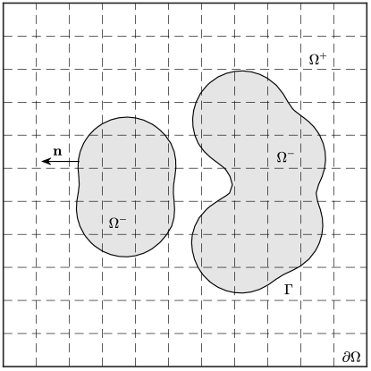
Figure 1: Schematic for the elliptic interface problem. $\Gamma$ is an interface that separates a cubical domain $\Omega$ with boundary $\partial\Omega$ into $\Omega^{+}$ and $\Omega^{-}$. The normal to the interface is denoted as $\mathbf{n}$. The dashed lines are the grid lines of the uniform mesh.

1.3 Interface Dynamics and Gradients

In applications that concern both such elliptic interface problems and moving intefaces, the velocity of the interface may depend on the gradient of the solution. This makes it imperative to accurately calculate not only the solution’s values, but its gradient as well macklin_evolving_2005 ; li_minimization_2009 ; zhou_variational_2014 . In fact, it is preferrable for errors to be measured under the infinity norm, to obtain accurate pointwise velocities that can be used in both front tracking methods and level-set methods for interface dynamics.

In our motivating biomolecular application, gradient descent on the free-energy functional can be used to capture the solute-solvent interface of interest dzubiella_coupling_2006 ; dzubiella_coupling_2006-1 . This introduces a time variable and interface dynamics into the originally static problem. Additionally, gradient descent in this case translates to a normal velocity that depends on the effective dielectric boundary force, which in turn depends on the jump of the normal derivative of the electrostatic potential at the interface li_minimization_2009 ; zhou_variational_2014 .

In another and perhaps better known example, the Stefan problem gibou_second-order-accurate_2002 is used to model an interface separating ice from water, where the interface moves when ice melts or water freezes. In simple terms, for a given configuration of the ice and water, an elliptic interface problem, with $\epsilon$ as thermal conductivity, can be solved for the temperature $u$. The interface between the ice and water then evolves due to this temperature, with its normal velocity depending on the jump in the normal derivative of the temperature.

From these considerations, we can finally formulate our goal: to accurately and efficiently solving elliptic interface problems with jump conditions for both solution and gradient.

1.4 Finite Difference Methods

Our approach towards this goal involves combining elements of CIM (the Coupling Interface Method) chern_coupling_2007 and Smereka’s grid-based work on second-order accurate discrete delta functions smereka_numerical_2006 . As both these methods are finite difference methods, our resulting method is also a finite difference method. We thus restrict our comparisons to other finite difference methods and, actually, specifically to CIM and its variations, which are among the top performing ones. We do note, however, that there are numerous other accurate approaches to elliptic interface problems with jump conditions, including boundary integral methods beale_grid-based_2004 ; zhong_implicit_2018 , finite element methods chen_finite_1998 ; huang_mortar_2002 ; li_new_2003 ; guo_gradient_2018 , finite volume methods bochkov_solving_2020 ; guittet_solving_2015 , and methods involving deep learning hu_discontinuity_2021 ; guo_deep_2022 .

Finite difference methods work on values given over an underlying grid. This, in general, leads to advantages of simplicity in aspects of accuracy and resolution, notably in the case of uniform grids. Thus, for each problem found in mathematics or sciences, one can find numerous finite difference methods available for solving it. Especially for interface representations and dynamics, there exist level-set methods osher_level_2003 ; osher_fronts_1988 , as well as phase-field methods du_chapter_2020 , that can capture moving curves and surfaces.

As discussed in chern_coupling_2007 , within finite difference methods, there are essentially three types of approaches: regularization, dimension unsplitting, and dimension splitting approaches. A regularizatation approach applies smoothing techniques to discontinuous coefficients, or regularization techniques to singular sources tornberg_numerical_2004 ; tornberg_regularization_2003 . An major example of this that is related to our problem of interest is the Immersed Boundary Method (IBM) peskin_immersed_2002 ; peskin_numerical-analysis_1977 . In dimension unsplitting approaches, finite difference methods are derived from local Taylor expansions in multi-dimensions. One popular method in this category is the Immersed Interface Method leveque_immersed_1994 and its various extensions, including the Maximum Principle Preserving Immersed Interface Method (MIIM)li_maximum_2001 , the Fast Immersed Interface Method (FIIM) li_fast_1998 , and the Augmented Immersed Interface Method (AIIM) li_accurate_2017 . For dimension splitting approaches, the finite difference methods are derived from Taylor expansions in each dimension. This category includes the Ghost Fluid Method liu_convergence_2003 ; liu_boundary_2000 ; fedkiw_non-oscillatory_1999 , the Explicit-jump Immersed Interface Method (EJIIM) wiegmann_explicit-jump_2000 , the Decomposed Immersed Interface Method (DIIM) berthelsen_decomposed_2004 , the Matched Interface Method (MIM) zhou_high_2006 , and the Coupling Interface Method (CIM) and its variation, Improved Coupling Interface Method (ICIM) chern_coupling_2007 ; shu_accurate_2014 ; shu_augmented_2010 . For a more detailed discussion on these different types, we refer readers to chern_coupling_2007 .

1.5 The Coupling Interface Method

Among these finite difference methods, CIM is one of the top ones in terms of accuracy, in both solutions values and gradients; ease of use; and detail of study (see chern_coupling_2007 ; shu_accurate_2014 ; shu_augmented_2010 ). The main approach of CIM involves generating at gridpoints accurate approximations of principal second-order derivatives, especially in the case where standard central differencing stencils would cross the interface and hence do not apply. These approximations can then be used to handle terms like the Laplacian, which is perhaps the most complex term in the PDE of our elliptic interface problem. The process consists, at a gridpoint of interest, of first using second-order central differencing in all dimensions that apply. In those that do not, this will be because the gridpoint lies next to the interface in that dimension. To handle this, CIM considers polynomial approximations on either side of the interface, in each such dimension, and connects them with jump conditions at the interface. This leads, in total, to a coupled linear system of equations to be solved for the principal second-order derivatives in terms of values at gridpoints. Note, this linear system also involves mixed second derivative terms, which are approximated to varying degrees of accuracy depending on available finite differencing schemes with stencils that does not cross the interface.

One version of this approach, called CIM1, chooses linear polynomials and lower-order approximations of mixed derivatives for a lower-order but widely applicable approach; another, called CIM2, chooses quadratic polynomials and higher-order approximations of mixed derivatives for a higher-order approach that, however, requires certain larger stencils. CIM is a hybrid of these that uses CIM2 approximations at points where the stencils allow, and CIM1 approximations at all other gridpoints, called exceptional points. Note, these exceptional points do commonly exist but, as noted in chern_coupling_2007 , not in great numbers, allowing CIM to be second-order accurate in solution values under the infinity norm. For gradients, however, this approach is only first-order accurate, especially at exceptional points.

The Improved Coupling Interface Method (ICIM) shu_accurate_2014 fixes this issue and achieves uniformly second-order accurate gradient by incorporating two recipes that handle exceptional points. One attempts to “shift”: at gridpoints where it is difficult to achieve a valid first-order approximation of the principal or mixed second-order derivative, the finite difference approximations at adjacent gridpoints, on the same side, are instead shifted over. The other attempts to “flip”: at some gridpoints, the signature of the domain (inside or outside) can be flipped, so that the usual second-order CIM2 discretization may apply, allowing for second-order accurate solutions and gradients for the flipped interface. Extrapolation from neighboring nonflipped gridpoints originally on the same side can then be used to recover the solutions and gradients of the original and desired interface. Note, the decisions on when to use shifts and when to use flips are listed in shu_accurate_2014 .

1.6 Our Proposed Method

We propose what can be considered a hybrid that we call the Compact Coupling Interface Method (CCIM). Our method combines elements of CIM chern_coupling_2007 and Smereka’s work on second-order accurate discrete delta functions by setting up an elliptic interface problem with interfacial jump conditions smereka_numerical_2006 . The use of Smereka’s setup, itself based on Mayo’s work in mayo_fast_1984 , allows us to remove the quadratic polynomial approximations of CIM2 and its need for two points on either side of the interface in a direction that crosses the interface, thus compacting the stencil and allowing more applicability in generating accurate principal second-order derivatives. Additional schemes are introduced to accurately handle mixed second-order derivatives by using more compact stencils on the same side or stencils from the opposite side, with the help of jump conditions, allowing for the removal of exceptional points. The result is that our constructed CCIM can approximate values and gradients of the solutions of elliptic interface problems with jump conditions with close to second-order accuracy in infinity norm for a variety interfaces, with observed advantages in robust convergence behavior in complex situations.

Note, while ICIM mostly improves on CIM2 through postprocessing, keeping the same coupling equations, which only includes the principal second-order derivatives, and similar finite difference stencils shu_accurate_2014 , our CCIM expands the coupling equations to include first-order derivatives as well, and utilizes more compact finite difference stencils, for the removal of additional exceptional points.

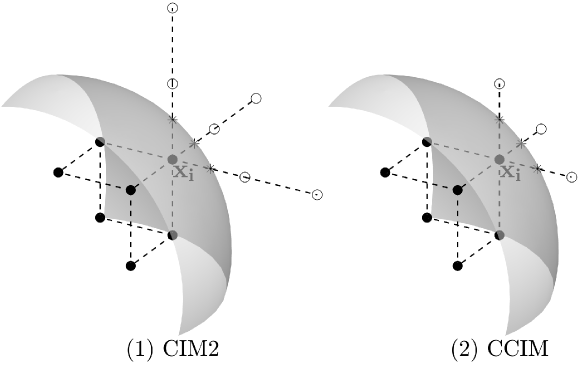
Figure 2: Examples of a (1) CIM2 stencil and a (2) CCIM stencil at $\mathbf{x_{i}}$. The circles and disks are grid points on different sides of the interface. The asterisks are the intersections of the surface and the grid lines. CIM2 stencils require 2 points on the same side of the interface in each dimension chern_coupling_2007 . Points that does not satisfy this requirement are handled in ICIM shu_accurate_2014 . The CCIM stencil requires fewer points so it’s more compact. Both CIM2 and CCIM need some extra grid points on the diagonal of $\mathbf{x_{i}}$ to approximate the mixed derivatives.

1.7 Outline

This paper is organized as follows. Section 2 outlines the derivation and algorithm of CCIM. In Section 3, we show the convergence tests in three dimensions on geometric surfaces and two complex protein surfaces. We also test our method on a moving surface driven by the jump of the gradient at the interface. Section 4 is the conclusion.

2 Method

In $d$ dimensions, let $\Omega=[-1,1]^{d}$ and discretize the domain uniformly with mesh size $h=2/N$, where $N$ is the number of subintervals on one side of the region $\Omega$. Let $\mathbf{i}=(i_{1},\ldots,i_{d})$ be the multi-index with $i_{k}=0,1,\ldots,N$ for $k=1,2,\ldots,d$. The grid points are denoted as ${\mathbf{x_{i}}}$ with $\mathbf{x}_{k}=-1+i_{k}h$. Let $\mathbf{e}_{k}$, $k=1,2,\ldots,d$ be the unit coordinate vectors. We also write $u(\mathbf{x_{i}})=u_{\mathbf{i}}$. Here we use $\Delta u$ for the Laplacian of $u$ and $\nabla^{2}u$ for the Hessian matrix of $u$. We assume that $\nabla^{2}u$ is symmetric. We use $\overline{\mathbf{x_{i}}\mathbf{x}_{\mathbf{i}+\mathbf{e}_{k}}}$ to denote the grid segment between ${\mathbf{x_{i}}}$ and $\mathbf{x}_{\mathbf{i}+\mathbf{e}_{k}}$, and assume that the interface intersects with any grid segment at most once.

Let ${\mathbf{x_{i}}}$ be a grid point at which we try to discretize the PDE. For notational simplicity, we drop the argument ${\mathbf{x_{i}}}$ and the dependency on $\mathbf{i}$ is implicit. We rewrite the PDE (1) at ${\mathbf{x_{i}}}$ as

$$-\sum_{k=1}^{d}\partialderivative{\epsilon}{x_{k}}\partialderivative{u}{x_{k}}-\epsilon\sum_{j=1}^{d}\partialderivative[2]{u}{x_{k}}+au=f$$ (4)

If $\mathbf{x}_{\mathbf{i}-\mathbf{e}_{k}}$, ${\mathbf{x_{i}}}$ and $\mathbf{x}_{\mathbf{i}+\mathbf{e}_{k}}$ are in the same region in each coordinate direction, then we call ${\mathbf{x_{i}}}$ an interior point, otherwise ${\mathbf{x_{i}}}$ is called an interface point. At interior points, standard central differencing gives a local truncation error of $\order{h^{2}}$ in $\mathbf{e}_{k}$ direction. Our goal is to construct finite difference schemes with $\order{h}$ local truncation error at interface points. The overall accuracy will still be second-order since the interface points belong to a lower dimensional set leveque_immersed_1994 . In this Section, we derive a first-order approximation for the term $\partialderivative*{u}{x_{k}}$ and $\partialderivative*[2]{u}{x_{k}}$ in terms of u-values on neighboring grid points. We denote the set of neighboring grid points of $\mathbf{i}$ as $B_{r}=\{\mathbf{j}\mid\norm{\mathbf{j}-\mathbf{i}}_{\infty}\leq r\}$ and call $r$ the radius of our finite difference stencil.

2.1 Dimension-by-dimension discretization

This section follows the derivation found in smereka_numerical_2006 . Along the coordinate direction $\mathbf{e}_{k}$, if the interface does not intersect the grid segment $\overline{\mathbf{x_{i}}\mathbf{x}_{\mathbf{i}+\mathbf{e}_{k}}}$, then by Taylor’s theorem,

$$u_{\mathbf{i}+\mathbf{e}_{k}}-u_{\mathbf{i}}=h\partialderivative{u}{x_{k}}+\frac{h^{2}}{2}\partialderivative[2]{u}{x_{k}}+\order{h^{3}}.$$ (5)

Suppose the interface intersects the grid segment $\overline{\mathbf{x_{i}}\mathbf{x}_{\mathbf{i}+\mathbf{e}_{k}}}$ at ${\mathbf{\hat{x}}_{k}}$. Let $\alpha_{k}=\norm{{\mathbf{\hat{x}}_{k}}-{\mathbf{x_{i}}}}/h$ and $\beta_{k}=1-\alpha_{k}$. Suppose ${\mathbf{x_{i}}}$ is located in $\Omega^{-}$. Denote the limit of $u(\mathbf{x})$ as $\mathbf{x}$ approaches ${\mathbf{\hat{x}}_{k}}$ from $\Omega^{-}$ by $u^{-}$ , and the limit from the other side by $u^{+}$ (see Fig 3). By Taylor’s theorem,

$$u_{\mathbf{i}} =u^{-}-\alpha h\partialderivative{u^{-}}{x_{k}}+\frac{(\alpha h)^{2}}{2}\partialderivative[2]{u^{-}}{x_{k}}+\order{h^{3}},$$ (6)

$$u_{\mathbf{i}+\mathbf{e}_{k}} =u^{+}+\beta h\partialderivative{u^{+}}{x_{k}}+\frac{(\beta h)^{2}}{2}\partialderivative[2]{u^{+}}{x_{k}}+\order{h^{3}}.$$

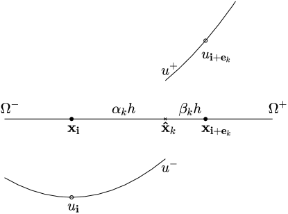
Figure 3: The interface intersects the grid segment $\overline{\mathbf{x_{i}}\mathbf{x}_{\mathbf{i}+\mathbf{e}_{k}}}$ at ${\mathbf{\hat{x}}_{k}}$. $u^{-}$ and $u^{+}$ are the limits of u at ${\mathbf{\hat{x}}_{k}}$ from $\Omega^{-}$ and $\Omega^{+}$. $u_{\mathbf{i}}$ and $u_{\mathbf{i}+\mathbf{e}_{k}}$ are approximated by Taylor’s expansion at the interface.

Subtract the above two equations and write the right-hand side in terms of jumps and quantities from $\Omega^{-}$:

$$u_{\mathbf{i}+\mathbf{e}_{k}}-u_{\mathbf{i}}=[u]+\beta h\left[\partialderivative{u}{x_{k}}\right]+h\partialderivative{u^{-}}{x_{k}}+\frac{h^{2}}{2}\beta^{2}\left[\partialderivative[2]{u}{x_{k}}\right]+\frac{h^{2}}{2}(\beta^{2}-\alpha^{2})\partialderivative[2]{u^{-}}{x_{k}}+\order{h^{3}}.$$ (7)

We can approximate components of $\gradient u^{-}$ and $\nabla^{2}u^{-}$ by

$$\partialderivative{u^{-}}{x_{i}}=\partialderivative{u}{x_{i}}+\alpha_{k}h\partialderivative{u}{x_{i}}{x_{k}}+\order{h^{2}},$$ (8)

$$\partialderivative{u^{-}}{x_{i}}{x_{k}}=\partialderivative{u}{x_{i}}{x_{k}}+\order{h}.$$ (9)

with $1\leq i\leq k\leq d$. Together with the given jump condition, $[u]=\tau$, (7) can be written as

$$u_{\mathbf{i}+\mathbf{e}_{k}}-u_{\mathbf{i}}=\tau+\beta h\left[\partialderivative{u}{x_{k}}\right]+h\left(\partialderivative{u}{x_{k}}+\alpha h\partialderivative[2]{u}{x_{k}}\right)$$ (10)

$$+\frac{h^{2}}{2}\beta^{2}\left[\partialderivative[2]{u}{x_{k}}\right]+\frac{h^{2}}{2}(\beta^{2}-\alpha^{2})\partialderivative[2]{u}{x_{k}}+\order{h^{3}}.$$

2.2 Coupling Equation

This section then sets up coupling equations following the work of chern_coupling_2007 . In (10), suppose we can approximate the jump $[\partialderivative*{u}{x_{k}}]$ and $[\partialderivative*[2]{u}{x_{k}}]$ in terms of $u_{\mathbf{j}}$, $\partialderivative*{u}{x_{k}}$ and $\partialderivative*[2]{u}{x_{k}}$, with $1\leq k\leq d$ and $\mathbf{j}\in B_{r}$ for some stencil radius $r$. Then in each coordinate direction, for $1\leq k\leq d$, we can write down two equations, (10) or (5), by considering the two grid segments $\overline{\mathbf{x_{i}}\mathbf{x}_{\mathbf{i}+s\mathbf{e}_{k}}}$ for $s=\pm 1$. In $d$ dimensions we have $2d$ equations and $2d$ unknowns: the first-order derivatives $\partialderivative*{u}{x_{k}}$ and the principal second-order derivatives $\partialderivative*[2]{u}{x_{k}}$ for $1\leq k\leq d$. This leads to a system of linear equations of the following form:

$$M\begin{pmatrix}\partialderivative{u}{x_{k}}\\ \partialderivative[2]{u}{x_{k}}\end{pmatrix}_{1\leq k\leq d}=\frac{1}{h^{2}}\begin{pmatrix}D_{k,s}u+b_{k,s}\end{pmatrix}_{1\leq k\leq d,s=\pm 1}+\order{h}$$ (11)

where $D_{k,s}u=D_{k,s}(u_{\mathbf{j}})$, $\mathbf{j}\in B_{r}$, is some linear function of neighboring $u$-values and $b_{k,s}$ is some constant. We call (11) the coupling equation and $M$ the coupling matrix. By inverting $M$, we can approximate $\partialderivative*{u}{x_{k}}$ and $\partialderivative*[2]{u}{x_{k}}$ in terms of $u$-values and obtain the finite different approximation of the PDE (4) at the interface point $\mathbf{x_{i}}$.

In the next few sections, we describe the ingredients to construct the coupling equation (11). In Section 2.3, we derive expressions to approximate the jump of the first-order derivatives $[\partialderivative*{u}{x_{k}}]$ in (10). In Section 2.4, we approximate the jump of the principal second-order derivatives $[\partialderivative*[2]{u}{x_{k}}]$ in (10). In Section 2.5, we discuss how to approximate the mixed derivatives, which is used to approximate $[\partialderivative*{u}{x_{k}}]$ and $[\partialderivative*[2]{u}{x_{k}}]$. In Section 2.6, we combine all the ingredients and describe our algorithm to obtain the coupling equation.

2.3 Approximation of $[\partialderivative*{u}{x_{k}}]$

Let $\mathbf{n}$ be the unit normal vector at the interface, and $\mathbf{s}_{1}$, …, $\mathbf{s}_{d-1}$ be the unit tangent vectors. The tangent vectors can be obtained by projecting the coordinate vectors onto the tangent plane. We can write

$$[\gradient u]=[\gradient u\cdot\mathbf{n}]\mathbf{n}+\sum_{j=1}^{d-1}[\gradient u\cdot\mathbf{s}_{j}]\mathbf{s}_{j}.$$ (12)

In the $\mathbf{e}_{k}$ coordinate direction, this gives

$$\left[\partialderivative{u}{x_{k}}\right]=[\gradient u\cdot\mathbf{n}](\mathbf{n}\cdot\mathbf{e}_{k})+\sum_{j=1}^{d-1}[\gradient u\cdot\mathbf{s}_{j}](\mathbf{s}_{j}\cdot\mathbf{e}_{k}).$$ (13)

In the following derivation, we use the following trick repeatedly to decouple the jump:

$$\left[\epsilon v\right]=\epsilon^{+}[v]+[\epsilon]v^{-}.$$ (14)

The jump condition $[\epsilon\nabla u\cdot\mathbf{n}]=\sigma$ can be rewritten as

$$[\gradient u\cdot\mathbf{n}]=\frac{1}{\epsilon^{+}}(\sigma-[\epsilon]\gradient u^{-}\cdot\mathbf{n}).$$ (15)

Substitute (15) into (13), together with with $[\gradient u\cdot\mathbf{s}_{k}]=\gradient\tau\cdot\mathbf{s}_{k}$, we have

$$\left[\partialderivative{u}{x_{k}}\right]=\frac{1}{\epsilon^{+}}(\sigma-[\epsilon]\gradient u^{-}\cdot\mathbf{n})(\mathbf{n}\cdot\mathbf{e}_{k})+\sum_{j=1}^{d-1}(\gradient\tau\cdot\mathbf{s}_{j})(\mathbf{s}_{j}\cdot\mathbf{e}_{k}).$$ (16)

Approximate $\gradient u^{-}$ by Taylor’s theorem (8), we get

$$\left[\partialderivative{u}{x_{k}}\right]=\frac{1}{\epsilon^{+}}\left(\sigma-[\epsilon]\sum_{j=1}^{d}\left(\partialderivative{u}{x_{j}}+\alpha_{k}h\partialderivative{u}{x_{j}}{x_{k}}\right)(\mathbf{n}\cdot\mathbf{e}_{j})\right)(\mathbf{n}\cdot\mathbf{e}_{k})$$ (17)

$$+\sum_{j=1}^{d-1}(\gradient\tau\cdot\mathbf{s}_{j})(\mathbf{s}_{j}\cdot\mathbf{e}_{k}).$$

Notice that the jump in the first-order derivative $[\partialderivative*{u}{x_{k}}]$ can be writen as linear combinations of the first-order derivatives $\partialderivative*{u}{x_{l}}$, $1\leq l\leq d$ and the second-order derivatives $\partialderivative*{u}{x_{l}}{x_{m}}$, $1\leq l\leq m$:

$$\left[\partialderivative{u}{x_{k}}\right]=L(\gradient u,\nabla^{2}u)+b.$$ (18)

where $L$ is some linear function and $b$ is some constant. Our goal is to approximate the mixed derivatives $\partialderivative*{u}{x_{k}}{x_{l}}$, $k\neq l$ in terms of the neighboring $u$-values $u_{\mathbf{j}}$, $\mathbf{j}\in B_{r}$, the first-order derivatives $\partialderivative*{u}{x_{k}}$, and the principal second-order derivatives $\partialderivative*[2]{u}{x_{k}}$, $1\leq k\leq d$ (see Section  2.4 and 2.5), which are the terms used in the coupling equation (11).

2.4 Approximation of $[\partialderivative*[2]{u}{x_{k}}]$

To remove the jump of the principal second-order derivatives $[\partialderivative*[2]{u}{x_{k}}]$, $k=1,2,\ldots,d$ in (10), we need to solve a system of linear equations, whose unknowns are all the jump of the principal and the mixed second-order derivatives.

The first set of equations are obtained by differentiating the interface boundary condition in the tangential directions. For $m=1,\cdots,d-1$ and $n=m,\cdots,d-1$, we get $d(d-1)/2$ equations

$$\gradient[\gradient u\cdot\mathbf{s}_{m}]\cdot\mathbf{s}_{n}=\gradient(\gradient\tau\cdot\mathbf{s}_{m})\cdot\mathbf{s}_{n}.$$ (19)

Expand every term, and with the help of (14) and (16), we get

$$\mathbf{s}_{n}^{T}[\gradient^{2}u]\mathbf{s}_{m}=\mathbf{s}_{n}^{T}\gradient^{2}\tau\mathbf{s}_{m}+\frac{1}{\epsilon^{+}}(\sigma-[\epsilon]\gradient u^{-}\cdot\mathbf{n})\mathbf{s}_{n}^{T}\gradient\mathbf{n}\mathbf{s}_{m}-(\gradient\tau\cdot\mathbf{n})\mathbf{s}_{n}^{T}\gradient\mathbf{n}\mathbf{s}_{m}.$$ (20)

By differentiating the jump of flux in the tangential directions, we get another $d-1$ equations for $m=1,\cdots,d-1$,

$$\gradient[\epsilon\gradient u\cdot\mathbf{n}]\cdot\mathbf{s}_{m}=\gradient\sigma\cdot\mathbf{s}_{m}.$$ (21)

After expansion,

$$\mathbf{s}_{m}^{T}[\gradient^{2}u]\mathbf{n} =\frac{1}{\epsilon^{+}}\gradient\sigma\cdot\mathbf{s}_{m}-\frac{[\epsilon]}{\epsilon^{+}}\mathbf{s}_{m}^{T}\nabla^{2}u^{-}\mathbf{n}-\frac{[\epsilon]}{\epsilon^{+}}\mathbf{s}_{m}^{T}\gradient\mathbf{n}\gradient u^{-}$$ (22)

$$-\sum_{k=1}^{d-1}(\gradient\tau\cdot\mathbf{s}_{k})\mathbf{s}_{m}^{T}\gradient\mathbf{n}\mathbf{s}_{k}-\frac{1}{(\epsilon^{+})^{2}}(\gradient\epsilon^{+}\cdot\mathbf{s}_{m})(\sigma-[\epsilon]\gradient u^{-}\cdot\mathbf{n})$$

$$-\frac{1}{\epsilon^{+}}[\gradient\epsilon\cdot\mathbf{s}_{m}](\gradient u^{-}\cdot\mathbf{n}).$$

The final equation comes from the jump of the PDE:

$$[-\gradient\cdot(\epsilon\gradient u)+au]=[f].$$ (23)

After expansion, we have

$$=-\left[\frac{f}{\epsilon}\right]+\frac{a^{+}}{\epsilon^{+}}\tau+\left[\frac{a}{\epsilon}\right]u^{-}$$ (24)

$$-\frac{1}{\epsilon^{+}}\sum_{k=1}^{d-1}(\gradient\tau\cdot\mathbf{s}_{k})(\gradient\epsilon^{+}\cdot\mathbf{s}_{k})-\left[\frac{\gradient\epsilon}{\epsilon}\right]\cdot\gradient u^{-}.$$

Combining (22), (20), and (24), we arrive at a system of linear equations whose unknowns are the jump of the second-order derivatives:

$$G\left(\left[\partialderivative{u}{x_{k}}{x_{l}}\right]\right)_{1\leq k\leq l\leq d}=L\left(u^{-},\gradient u^{-},\nabla^{2}u^{-}\right)+b.$$ (25)

where $G$ is a matrix that only depends on the normal and the tangent vectors, $L$ stands for some general linear function and $b$ stands for some constant. In two and three dimensions, through a direct calculation, the absolute value of the determinant of $G$ is 1.

As an example, in two dimensions, let $\mathbf{s}=[s_{1},s_{2}]^{T}$ and $\mathbf{n}=[n_{1},n_{2}]^{T}$, and assume that $\epsilon(\mathbf{x})$ is a piecewise constant function, then the system of linear equations is given by

$$\begin{pmatrix}s_{1}^{2}&s_{2}^{2}&2s_{1}s_{2}\\ s_{1}n_{1}&s_{2}n_{2}&s_{1}n_{2}+s_{2}n_{1}\\ 1&1&0\\ \end{pmatrix}\begin{pmatrix}[u_{xx}]\\ [u_{yy}]\\ [u_{xy}]\\ \end{pmatrix}=$$ (26)

$$\begin{pmatrix}\mathbf{s}^{T}\nabla^{2}\tau\mathbf{s}+\frac{1}{\epsilon^{+}}\left(\sigma-[\epsilon]\nabla u^{-}\cdot\mathbf{n}\right)\mathbf{s}^{T}\gradient\mathbf{n}\mathbf{s}-(\gradient\tau\cdot\mathbf{n})\mathbf{s}^{T}\gradient\mathbf{n}\mathbf{s}\\ \frac{1}{\epsilon^{+}}\gradient\sigma\cdot\mathbf{s}-\frac{[\epsilon]}{\epsilon^{+}}(\mathbf{s}^{T}\nabla^{2}u^{-}\mathbf{n}+\mathbf{s}^{T}\gradient\mathbf{n}\gradient u^{-})-(\gradient\tau\cdot\mathbf{s})\mathbf{s}^{T}\gradient\mathbf{n}\mathbf{s}\\ -[\frac{f}{\epsilon}]+\frac{a^{+}}{\epsilon^{+}}\tau-[\frac{a}{\epsilon}]u^{-}\\ \end{pmatrix}.$$

By Taylor’s theorem as in (5) (8), and (9), $u^{-}$, $\gradient u^{-}$ and $\nabla^{2}u^{-}$ can all be approximated by $u_{\mathbf{j}}$, $\mathbf{j}\in B_{r}$ and components of $\gradient u$ and $\nabla^{2}u$ at the grid point. Therefore, after substitution, (25) has the form

$$G\left(\left[\partialderivative{u}{x_{k}}{x_{l}}\right]\right)_{1\leq k\leq l\leq d}=L\left(u_{\mathbf{j}},\gradient u,\nabla^{2}u\right)+b.$$ (27)

where $\mathbf{j}\in B_{r}$. If we could approximate the mixed derivatives $\partialderivative*{u}{x_{k}}{x_{l}}$, $k\neq l$ in terms of $u_{\mathbf{j}}$, $\mathbf{j}\in B_{r}$, $\partialderivative*{u}{x_{k}}$, $\partialderivative*[2]{u}{x_{k}}$ and $[\partialderivative*{u}{x_{k}}{x_{l}}]$, $1\leq k<l\leq d$ (See Section 2.5), then by re-arranging the equations and solving the linear systems, the jump of all the second-order derivatives $[\partialderivative*{u}{x_{k}}{x_{l}}]$, $1\leq k\leq l\leq d$, can be approximated in terms of $u_{\mathbf{j}}$, $\mathbf{j}\in B_{r}$, $\partialderivative*{u}{x_{k}}$, $\partialderivative*[2]{u}{x_{k}}$, $1\leq k\leq d$, which are the terms used in the coupling equation (11). By back substitution, all the mixed derivatives $\partialderivative*{u}{x_{k}}{x_{l}}$, $1\leq k\leq d$, can also be approximated by these terms. Then the jump of the first-order derivative $[\partialderivative*{u}{x_{k}}]$ (18) can be approximated by these terms. Next, we describe how to approximate the mixed derivatives.

2.5 Approximation of the mixed derivative

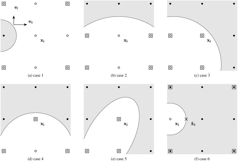
Figure 4: Approximation of the mixed derivative $\partialderivative*{u}{x_{k}}{x_{l}}$ at ${\mathbf{x_{i}}}$. The circles and disks are grid points in $\Omega^{-}$ and $\Omega^{+}$. The $u$-values at the squares are used to approximate the mixed derivative. Case 1 is the usual central difference. Case 2 and 3 are biased difference. Case 4 uses the first-order derivatives at at ${\mathbf{x_{i}}}$. Case 5 uses the first-order and the second-order derivatives at at ${\mathbf{x_{i}}}$. Case 6 uses the jump $[\partialderivative*{u}{x_{k}}{x_{l}}]$ at ${\mathbf{\hat{x}}_{k}}$ and the mixed second-order derivative on the other side at $\mathbf{x}_{\mathbf{i}+\mathbf{e}_{k}}$, which is approximated by central difference.

Depending how the interface intersects the grid, different schemes are needed to approximate the mixed derivative $\partialderivative*{u}{x_{k}}{x_{l}}$, $k\neq l$ at ${\mathbf{x_{i}}}$. Notice that we are allowed to make use of the first-order and the second-order derivatives, as they are the variables in the coupling equation (11). Though any $\order{h}$ approximation suffices, we prefer schemes with smaller local truncation error. Therefore, in all the following formula, we also compute the $\order{h}$ term explicitly. In Fig. 4, we demonstrate examples of different scenarios. In Fig. 4 case 1, we use the usual central difference formula,

$$\partialderivative{u}{x_{k}}{x_{l}}=\frac{1}{4h^{2}}\left(u_{\mathbf{i}+\mathbf{e}_{k}+\mathbf{e}_{l}}-u_{\mathbf{i}-\mathbf{e}_{k}+\mathbf{e}_{l}}-u_{\mathbf{i}+\mathbf{e}_{k}-\mathbf{e}_{l}}+u_{\mathbf{i}-\mathbf{e}_{k}-\mathbf{e}_{l}}\right)+\order{h^{2}}.$$ (28)

We can also use biased differencing as in Fig. 4 case 2 and case 3:

$$\partialderivative{u}{x_{k}}{x_{l}} =\frac{1}{2h^{2}}\left(u_{\mathbf{i}+\mathbf{e}_{k}}-u_{\mathbf{i}+\mathbf{e}_{k}-\mathbf{e}_{l}}-u_{\mathbf{i}-\mathbf{e}_{k}}+u_{\mathbf{i}-\mathbf{e}_{k}-\mathbf{e}_{l}}\right)$$ (29)

$$+\frac{1}{2}h\partialderivative{u}{x_{k}}{x_{l}^{2}}+\order{h^{2}}$$

$$\partialderivative{u}{x_{k}}{x_{l}} =\frac{1}{h^{2}}(u_{\mathbf{i}}-u_{\mathbf{i}-\mathbf{e}_{k}}-u_{\mathbf{i}-\mathbf{e}_{l}}+u_{\mathbf{i}-\mathbf{e}_{k}-\mathbf{e}_{l}})$$ (30)

$$+\frac{1}{2}h\left(\partialderivative{u}{x_{k}}{x_{l}^{2}}+\partialderivative{u}{x_{k}^{2}}{x_{l}}\right)+\order{h^{2}}$$

In case 4, we can make use of the first-order derivatives

$$\partialderivative{u}{x_{k}}{x_{l}} =\frac{1}{2h^{2}}\left(2h\partialderivative{u}{x_{k}}+u_{\mathbf{i}+\mathbf{e}_{k}-\mathbf{e}_{l}}-u_{\mathbf{i}-\mathbf{e}_{k}-\mathbf{e}_{l}}\right)$$ (31)

$$+\frac{1}{2}h\left(\partialderivative{u}{x_{k}}{x_{l}^{2}}+\frac{1}{3}\partialderivative[3]{u}{x_{k}}\right)+\order{h^{2}}$$

In case 5, we can make use of the first-order and the principal second-order derivatives

$$\partialderivative{u}{x_{k}}{x_{l}} =\frac{1}{h^{2}}\left(h\partialderivative{u}{x_{k}}-\frac{h^{2}}{2}\partialderivative[2]{u}{x_{k}}-u_{\mathbf{i}-\mathbf{e}_{l}}+u_{\mathbf{i}-\mathbf{e}_{k}-\mathbf{e}_{l}}\right)$$ (32)

$$+\frac{1}{2}h\left(\partialderivative{u}{x_{k}}{x_{l}^{2}}+\partialderivative{u}{x_{k}^{2}}{x_{l}}+\frac{1}{3}\partialderivative[3]{u}{x_{k}}\right)+\order{h^{2}}$$

In Fig. 4 case 6, when there are not enough grid points on the same side, we can make use of the mixed derivative on the other side of the interface and the jump of the mixed derivative

$$\partialderivative{u}{x_{k}}{x_{l}} =\partialderivative{u}{x_{k}}{x_{l}}\/(\mathbf{x}_{\mathbf{i}+\mathbf{e}_{k}})-\left[\partialderivative{u}{x_{k}}{x_{l}}\right]_{\mathbf{\hat{x}}_{k}}+\order{h}$$ (33)

where $\partialderivative*{u}{x_{k}}{x_{l}}\/(\mathbf{x_{i}}+h\mathbf{e}_{k})$ can be approximated by $u$-values on the other side of the interface using central difference as in case 1 to 3. In case 6, the finite difference stencil will have a radius $r=2$, as $u$-values of more than one grid point away are used. In all the other cases, we have $r=1$. In contrast, for CIM2 and ICIM, $r\geq 2$.

Though not illustrated in Fig. 4, it’s also possible to approximate the mixed derivative at $\mathbf{x_{i}}$ by the mixed derivative at any of its direct neighbor that is on the same side of the region, and can be approximated using only $u$-values:

$$\partialderivative{u}{x_{k}}{x_{l}}=\partialderivative{u}{x_{k}}{x_{l}}\/(\mathbf{x}_{\mathbf{i}+s\mathbf{e}_{m}})+\order{h},$$ (34)

where $s=\pm 1$ and $1\leq m\leq d$. This is similar to the “shifting” strategy used in ICIM shu_accurate_2014 . If $m=k$ or $l$, that is, we are shifting in the $kl$-plane, then the stencil have a radius $r=2$. Otherwise, we are shifting out of the $kl$-plane, and the stencil has a radius $r=1$. Therefore, shifting out of plane is preferred for a more compact stencil.

By approximating the mixed derivatives $\partialderivative*{u}{x_{k}}{x_{l}}$, $1\leq k<l\leq d$ in terms of $u_{\mathbf{j}}$, $\mathbf{j}\in B_{r}$, $\partialderivative*{u}{x_{k}}$, $\partialderivative*[2]{u}{x_{k}}$ and $[\partialderivative*{u}{x_{k}}{x_{l}}]$ (if case 6 is needed), $1\leq k\leq d$, we can write the right-hand side of (27) in terms of $u_{\mathbf{j}}$, $\partialderivative*{u}{x_{k}}$ and $\partialderivative*[2]{u}{x_{k}}$, $1\leq k\leq d$, thus eliminating the mixed derivatives. Then by solving the linear system (27), the jump of second derivatives $[\partialderivative*[2]{u}{x_{k}}]$ and $[\partialderivative*{u}{x_{k}}{x_{l}}]$ can be approximated in terms of $u_{\mathbf{j}}$, $\partialderivative*{u}{x_{k}}$ and $\partialderivative*[2]{u}{x_{k}}$, $1\leq k\leq d$. Therefore, we can eliminate $[\partialderivative*[2]{u}{x_{k}}]$ in (10). By back substitution of $[\partialderivative*{u}{x_{k}}{x_{l}}]$ into (33), all the approximations of the mixed derivative (case 1 to 6) are written in terms of $u_{\mathbf{j}}$, $\partialderivative*{u}{x_{k}}$ and $\partialderivative*[2]{u}{x_{k}}$, $1\leq k\leq d$. Therefore, we can also eliminate $[\partialderivative*{u}{x_{k}}]$ in (10). As promised in Section 2.2, we can now assemble the coupling equation.

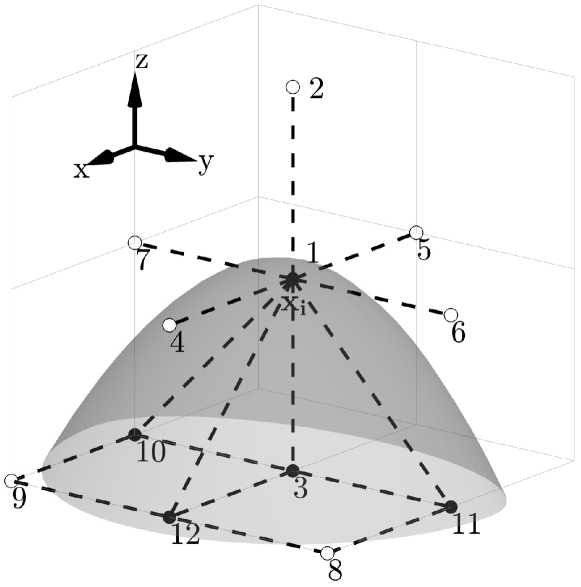
Figure 5: An example of CCIM stencil at $\mathbf{x_{i}}$. The grid points in the stencil are labelled from 1 to 12. The disks and the circles are the grid points outside and inside the surface. (1,10,11) are used to approximate $u_{yz}(\mathbf{x_{i}})$ (see Fig. 4 case 4). (1, 3, 12) are used to approximate $u_{zx}(\mathbf{x_{i}})$ (Fig. 4 case 5). (8, 9, 10, 11) can be used to approximate $u_{xy}(\mathbf{x_{i}})$. Alternatively, $u_{xy}(\mathbf{x_{i}})$ can be approximated by using $u_{xy}$ at the other side (any one of 2, 4, 5, 6 or 7) and the jump condition (see Fig. 4 case 6).

Multiple schemes to approximate the mixed derivatives might be available at the same grid point. We would like the scheme to be simple, compact and accurate. For simplicity, we prefer schemes that only use $u$-values, as in case 1, 2 and 3. For compactness, we want to have a smaller radius $r$ for our finite difference stencil. Therefore case 6 is the least preferable. And when shifting is used, we prefer shifting out-of-plane than shifting in-plane . For accuracy, we look at the $\order{h}$ of the local truncation error. Central differencing (case 1) is preferred over biased differencing (and case 2 over case 3). When the derivatives are used, case 4 is preferred over case 5. And shifting will leads to larger local truncation error compared with case 1 to 5. However, case 3 or case 4 has similar local truncation error. Another consideration for accuracy is the condition number of the coupling equation. Solving a linear system with large condition number is prone to large numerical errors. Therefore, in cases where both case 3 and case 4 are available, we choose the scheme that leads to the coupling matrix with a smaller estimated condition number hager_condition_1984 , and the effect is shown in Section 3. As a summary, here is how we rank the schemes: case 1; case 2; case 3 or case 4, whichever leads to coupling matrix with smaller estimated condition number; case 5; shifting (out-of-plane preferred over in-plane); case 6.

Though we can construct surfaces for a specific grid size such that none of the above schemes works, for smooth surfaces we can refine the grid such that the above schemes suffice. In addition, we note that case 5 and case 6 can be removed by refining the grid, while case 4 cannot shu_accurate_2014 .

2.6 Algorithm

We describe our method to obtain the coupling equation at an interface point in algorithmic order in Algorithm 1. Once we have the coupling equations (11), by inverting the coupling matrix, $\partialderivative*{u}{x_{k}}$ and $\partialderivative*[2]{u}{x_{k}}$, $1\leq k\leq d$ can be approximated by linear functions of $u_{\mathbf{j}}$, $\mathbf{j}\in B_{r}$

Algorithm 1 Coupling equation at an interface point ${\mathbf{x_{i}}}$

1:  for $1\leq k\leq d$ do

2:     for $s=\pm 1$ do

3:        if the interface intersects $\overline{\mathbf{x_{i}}\mathbf{x}_{\mathbf{i}+s\mathbf{e}_{k}}}$ at ${\mathbf{\hat{x}}_{k}}$ then

4:           for $1\leq j\leq d$, $j\neq k$ do

5:              Approximate the mixed derivative $\partialderivative*{u}{x_{k}}{x_{j}}$ in terms of $u_{\mathbf{j}}$, $\mathbf{j}\in B_{r}$, $\partialderivative*{u}{x_{l}}$, $\partialderivative*[2]{u}{x_{l}}$, $1\leq l\leq d$, and $[\partialderivative*{u}{x_{k}}{x_{j}}]$ (if we need to use information on the other side, as in Fig.4 case 6. See Section 2.5).

6:           end for

7:           Differentiate the jump conditions and obtain a system of equations of the jump of second derivatives (27). Plug in the approximation of the mixed derivatives. Invert the matrix $G$, then $[\partialderivative*{u}{x_{k}}{x_{j}}]$, $1\leq k\leq j\leq d$, are approximated in terms of $u_{\mathbf{j}}$, $\mathbf{j}\in B_{r}$, $\partialderivative*{u}{x_{j}}$, $\partialderivative*[2]{u}{x_{j}}$, $1\leq j\leq d$.

8:           By back substitution, the mixed derivative $\partialderivative*{u}{x_{k}}{x_{j}}$ (if case 6 exists) and thus $[\partialderivative*{u}{x_{k}}]$ (17) can be expressed in terms of $u_{\mathbf{j}}$, $\mathbf{j}\in B_{r}$, $\partialderivative*{u}{x_{j}}$, $\partialderivative*[2]{u}{x_{j}}$, $1\leq j\leq d$.

9:           Substitute the expressions for $[\partialderivative*{u}{x_{k}}]$ and $[\partialderivative*[2]{u}{x_{k}}]$ into (10). After rearrangement, this gives one row of the coupling equations (11).

10:        else

11:           Direct application of Taylor’s theorem (5) gives one row of the coupling equations (11).

12:        end if

13:     end for

14:  end for

To get more stable convergence results, at grid points where case 1 and 2 not available, but case 3 and 4 are available, we use the algorithm to obtain two systems of coupling equations, and choose the system with a smaller estimated condition number of the coupling matrix. The effect of this criterion is demonstrated in Section 3.1.

3 Numerical results

We test our method in three dimensions with different surfaces. The first set of tests contains six geometric surfaces that are used in shu_accurate_2014 . And the second set of tests uses two complex biomolecular surfaces. These two sets are compared with our implementation of ICIM shu_accurate_2014 with the same setup. As tests in shu_accurate_2014 do not include the $a(\mathbf{x})$ term, the third set of tests are the same six geometric surfaces with the $a(\mathbf{x})$ term. The last test is a sphere expanding under a normal velocity given by the derivative of the solution in normal direction. Let $u_{e}$ be the exact solution of (1), and $u$ be the numerical solution. For tests with a static interface, we look at the maximum error of the solution at all grid points, denoted as $\norm{u_{e}-u}_{\infty}$, and the maximum error of the gradient at all the intersections of the interface and the grid lines, denoted as $\norm{\gradient u_{e}-\gradient u}_{\infty,\Gamma}$. For the expanding sphere, we look at the maximum error and the Root Mean Square Error (RMSE) of the radius at all the intersections of the interface and the grid lines. All the tests are performed on a 2017 iMac with 3.5 GHz Intel Core i5 and 16GB memory. We use the AMG method implemented in the HYPRE library falgout_hypre_2002 to solve the sparse linear systems to a tolerance of $10^{-9}$.

3.1 Example 1

We test several geometric interfaces as in shu_accurate_2014 . The surfaces are shown in Fig.6. Their level set functions are given below:

• Eight balls: $\phi(x,y,z)=\min_{0\leq k\leq 7}\sqrt{(x-x_{k})^{2}+(y-y_{k})^{2}+(z-z_{k})^{2}}-0.3$, where $(x_{k},y_{k},z_{k})=((-1)^{\lfloor k/4\rfloor}\times 0.5,(-1)^{\lfloor k/2\rfloor}\times 0.5,(-1)^{k}\times 0.5)$

• Ellipsoid: $\phi(x,y,z)=2x^{2}+3y^{2}+6z^{2}-1.3$

• Peanut: $\phi(x,y,z)=\phi(r,\theta,\psi)=r-0.5-0.2\sin(2\theta)\sin(\psi)$

• Donut: $\phi(x,y,z)=(\sqrt{x^{2}+y^{2}}-0.6)^{2}+z^{2}-0.4^{2}$

• Banana: $\phi(x,y,z)=(7x+6)^{4}+2401y^{4}+3601.5z^{4}+98(7x+6)^{2}(y^{2}+z^{2})+4802y^{2}z^{2}-94(7x+6)^{2}+3822y^{2}-4606z^{2}+1521$

• Popcorn:

  $$\phi(x,y,z) =\sqrt{x^{2}+y^{2}+z^{2}}-r_{0}$$

  $$-\sum_{k=0}^{11}\exp(25((x-x_{k})^{2}+(y-y_{k})^{2}+(z-z_{k})^{2}))$$

  where

  $$(x_{k},y_{k},z_{k})$$

  $$=\frac{r_{0}}{\sqrt{5}}\left(2\cos\left(\frac{2k\pi}{5}-\lfloor\frac{k}{5}\rfloor\right),2\sin\left(\frac{2k\pi}{5}-\lfloor\frac{k}{5}\rfloor\right),(-1)^{\lfloor\frac{k}{5}\rfloor}\right),0\leq k\leq 9$$

  $$=r_{0}(0,0,(-1)^{k-10}),10\leq k\leq 11.$$

The exact solution and the coefficient are given by

$$u_{e}(x,y,z)=\begin{cases}xy+x^{4}+y^{4}+xz^{2}+\cos(2x+y^{2}+z^{3})&\text{if $(x,y,z)\in\Omega^{+}$}\\ x^{3}+xy^{2}+y^{3}+z^{4}+\sin(3(x^{2}+y^{2}))&\text{if $(x,y,z)\in\Omega^{-}$}\end{cases}$$ (35)

and

$$\epsilon(x,y,z)=\begin{cases}80&\text{if $(x,y,z)\in\Omega^{+}$}\\ 2&\text{if $(x,y,z)\in\Omega^{-}$}\end{cases}.$$ (36)

The source term and the jump conditions are calculated accordingly.

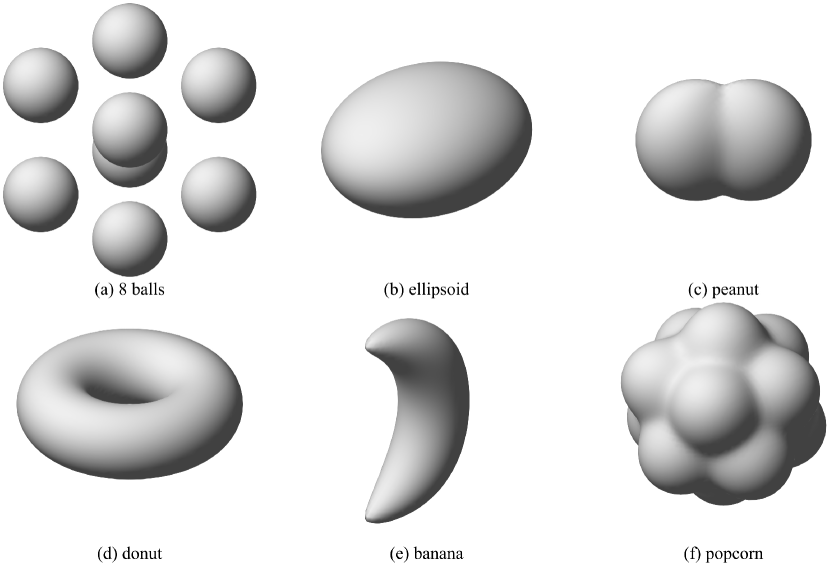
Figure 6: The six interfaces (a) eight balls; (b) ellipsoid; (c) peanut; (d) donut; (e) banana; (f) popcorn

Fig 7 shows the convergence result of the six interfaces. The convergence of the solution at grid points is second-order, and the convergence of the gradient at the interface is close to second-order.

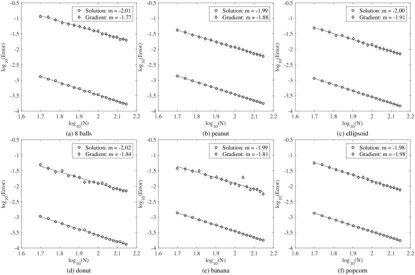
Figure 7: The log-log plot of the error versus $N$ for the six surfaces. In each figure, N ranges from 50 to 140 with the increment $\Delta N=5$. Circles are the maximum errors of the solution $\norm{u_{e}-u}_{\infty}$. Diamonds are the maximum errors of the gradient at interface $\norm{\gradient u_{e}-\gradient u}_{\infty,\Gamma}$. $m$ is the slope of the fitting line.

Next we demonstrate the effect of choosing the approximation schemes for the mixed derivatives based on the estimated condition numbers of the coupling matrices. As mentioned in Section 2.5, when both case 3 and case 4 are available to approximate the mixed derivatives, we choose the scheme that gives a smaller estimated condition number of the coupling matrix. We denote this scheme as “CCIM”. Alternatively, we can fix the order of preference for different methods. In “scheme 1”, we always prefer case 4 to case 3. Fig. 8 demonstrates the effect of this decision using the banana shape surface as an example. For different $N$ and for both schemes, Fig. 8(a) plots the maximum condition numbers (not estimated) of all the coupling matrices, and Fig. 8(b) plots the convergence results of these two schemes. From Fig. 8(a), we can see that the maximum condition numbers in CCIM are almost always smaller than those in scheme 1, except at $N=75$. This is expected as we choose the scheme with a smaller estimated condition number using the algorithm in hager_condition_1984 , which provides good estimation instead of the exact conditional number, which is costlier to compute. As shown in Fig. 8(b), for most of the tests, CCIM and scheme 1 have roughly the same maximum error. We noticed that for $N=110$, with scheme 1, at the interface point with the maximum error in the gradient, the coupling matrix has an exceptionally large condition number. By choosing the method with a smaller estimated condition number, we can get smaller error and obtain more stable convergence result in the gradient. If we prefer case 3 to case 4, then the results are similar to scheme 1: at some grid points large condition number is correlated to large error, and CCIM has more stable convergence behavior.

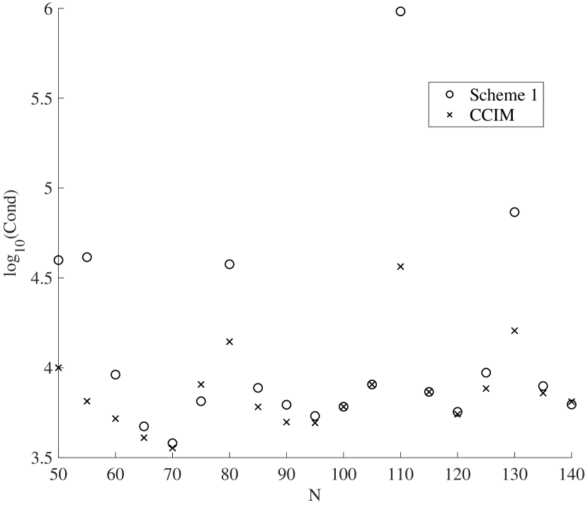
(a) maximum condition number

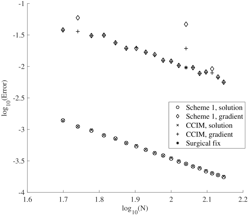
(b) Convergence

Figure 8: Comparison of maximum condition numbers and convergence results with banana surface between scheme 1 and CCIM. In scheme 1, case 4 is preferred to case 3. In CCIM, case 3 and case 4 are chosen based on estimated condition numbers of the coupling matrices. (a) The maximum condition number of coupling matrices with different methods. (b) Log-log plot of the maximum errors in solution and gradient at the interface. The relatively large error at $N=110$ for CCIM can be reduced by a surgical fix that choose the stencil with a smaller local truncation error.

Though we can get a more stable convergence behavior by considering the condition number of the coupling matrices, there is a small bump of the error of the gradient for the banana interface at $N=110$ in Fig. 8(b). A detailed analysis of the error reveals that it is caused by relatively large local truncation error when approximating $u_{xz}$. Fig. 9 shows the contour plot of the mixed derivative $u_{xz}$. Notice that $u_{xz}$ changes rapidly along the northeast direction. However, due to the alignment of the surface with the grid, at $\mathbf{x}_{i,k}$, our algorithm uses the 4-point stencil $\mathbf{x}_{i,k}$, $\mathbf{x}_{i-1,k}$, $\mathbf{x}_{i,k-1}$ and $\mathbf{x}_{i-1,k-1}$ to approximate $u_{xz}(\mathbf{x}_{i,k})$ and has a local truncation error 0.160723. If we use the three point stencil $\mathbf{x}_{i,k}$, $\mathbf{x}_{i-1,k}$, $\mathbf{x}_{i-1,k+1}$, the local truncation error would be 0.041853, and the coupling matrix does not have large condition number. With this surgical fix, the final error would be in line with the rest of the data points, as shown in Fig 8(b) at N = 110, marked as “Surgical fix”. This type of outliers happens rarely and does not affect the overall order of convergence. We apply this surgical fix only at this specific grid point to demonstrate a possible source of large error.

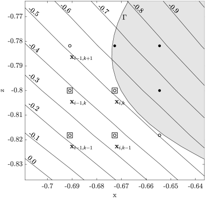
Figure 9: Contour of $u_{xz}$ at the grid point where the maximum error in the gradient occurs for the banana interface at $N=110$. The disks and the circles are grid points outside and inside the surface. Grid points marked with squares (Fig. 4 case 3) are used to approximate $u_{xz}$ at $\mathbf{x}_{i,k}$ due to its simplicity, while the three points stencil (Fig. 4 case 4) with $\mathbf{x}_{i,k}$, $\mathbf{x}_{i-1,k}$, $\mathbf{x}_{i-1,k+1}$ has a smaller local truncation error.

In summary, though the overall order of convergence is second-order no matter which scheme is used to approximate the mixed second-order derivatives, a relatively large error can be caused by a large condition number of the coupling matrix, or a large local truncation error when approximating the mixed second-order derivative. When different schemes to approximate the mixed second-order derivatives are available, ideally we prefer the scheme that produces smaller local truncation error and smaller condition number of the coupling matrix. However, these two goals might be incompatible sometimes. It’s time consuming to search through all the available schemes and find the one that leads the smallest condition number of the coupling matrix. It’s also difficult to tell a priori which scheme gives smaller local truncation error. Therefore we try to find a middle ground by only considering the condition number when both case 1 and 2 are not available but case 3 and case 4 are available.

The resulting linear system for the PDE is sparse and asymmetric, and can be solved with any “black-box” linear solvers. Fig. 10 shows the log-log plot for the number of iterations versus $N$. We used BiCGSTAB with ILU preconditioner and Algebraic Multigrid Method (AMG), both are implemented in the HYPRE library falgout_hypre_2002 . The number of iterations grows linearly with $N$ for BiCGSTAB and sub-linearly for AMG. Though AMG has better scaling property, for the range of $N$ in Fig 10, both solvers take approximately the same sCPU time.

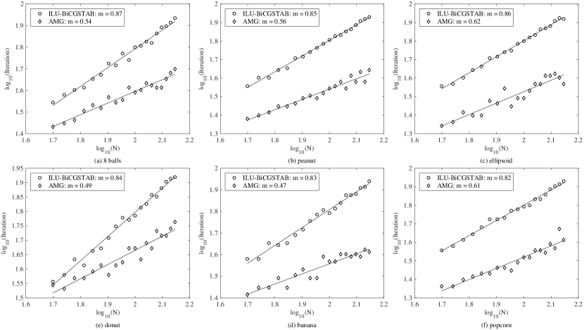
Figure 10: The log-log plot of the number of iterations versus $N$ for the six surfaces. In each figure, N ranges from 50 to 140 with the increment $\Delta N=5$. Circles are the numbers of iterations using BiCGSTAB with ILU preconditioner. Diamonds are the numbers of iterations using AMG. $m$ is the slope of the fitting line. Though AMG has better scaling (smaller $m$), both solvers take approximately the same cpu time in this range of $N$.

3.2 Example 2

Next we test our method on two complex molecular surfaces and compare CCIM with our implementation of ICIM shu_accurate_2014 . The solvent accessible surface describes the interface between solute and solvent. Such interfaces are complex and important in applications. We construct the surfaces as in shu_accurate_2014 : from the PDB file of 1D63 brown_crystal_1992 and MDM2 kussie_structure_1996 , we use the PDB2PQR dolinsky_pdb2pqr_2004 software to assign charges and radii using the AMBER force field. The PQR files contain information of the positions $\mathbf{p_{i}}$ and radii $r_{i}$ of the atoms. We scale the positions and radii such that the protein fit into our computation box. Then we construct the level set function of the interface as the union of smoothed bumps:

$$\phi(\mathbf{x})=c-\sum_{i}\chi_{\eta}(r_{i}-\norm{\mathbf{x}-\mathbf{p_{i}}}),$$ (37)

where $\chi_{\eta}$ is a smoothed characteristic function

$$\chi_{\eta}=\frac{1}{2}\left(1+\tanh\left(\frac{x}{\eta}\right)\right).$$ (38)

The molecule 1D63 has 486 atoms and has a double-helix shape, as shown in Fig. 11(a). MDM2 has 1448 atoms, and the surface has a deep pocket to which other proteins can bind, as shown in Fig 12(a). We also implement ICIM shu_accurate_2014 and compare the convergence results between CCIM and ICIM in Fig. 11 and Fig. 12.

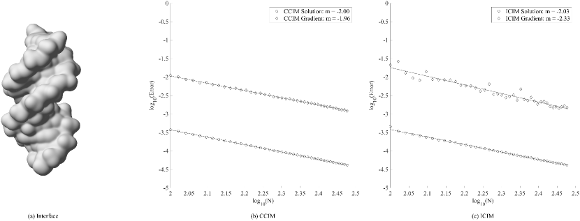
Figure 11: Convergence result for 1D63 interface with $c=0.25$ and $\eta=1/40$. (a) The smooth surface of 1D63. (b) log-log plot of error by CCIM. (b) log-log plot of error by ICIM. $N$ ranges from 100 to 340 with the increment $\Delta N=5$.

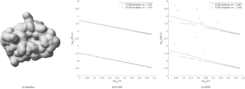
Figure 12: Convergence result for MDM2 interface with $c=0.25$ and $\eta=1/30$. (a) The smooth surface of MDM2. (b) log-log plot of error by CCIM. (b) log-log plot of error by ICIM. $N$ ranges from 100 to 340 with the increment $\Delta N=5$.

As shown in Fig. 11 and Fig. 12, compared with our implementation of ICIM, the convergence results of CCIM is very robust even for complex interfaces. There is little fluctuation in the convergence results. In our ICIM implementation, the order of convergence exceeds second-order because large errors at coarse grid points skew the fitting line to have a more negative slope. The results demonstrate the advantage of the compactness in our CCIM formulation when dealing with complex surfaces.

3.3 Example 3

We also test our problem with the same exact solution (35) and coefficients (36), but with an $a(x,y,z)$ term, which is not handled in CIM and ICIM. We take

$$a(x,y,z)=\begin{cases}2\sin(x)&\text{if $(x,y,z)\in\Omega^{-}$}\\ 80\cos(z)&\text{if $(x,y,z)\in\Omega^{+}$}.\end{cases}$$ (39)

As shown in Fig. 13, the convergence result is very similar to those without the $a(x,y,z)$ term.

Figure 13: The log-log plot of error with $a(\mathbf{x})$ term versus $N$ for the six surfaces. In each figure, N ranges from 50 to 140 with the increment $\Delta N=5$.

3.4 Example 4

In this example we look at the evolution of an interface driven by the jump of the normal derivative of the solution using the level set method osher_level_2003 . Suppose the surface $\Gamma$ is evolved with normal velocity $v_{n}=[\gradient u\cdot n]$. $\phi=\phi(\mathbf{x},t)$ is a level set function representing the evolving surface $\Gamma=\Gamma(t)$, i.e., $\Gamma(t)=\{\mathbf{x}\mid\phi(\mathbf{x},t)=0\}$. The dynamics of the interface is given by the level set equation,

$$\phi_{t}+v_{n}|\gradient\phi|=0.$$ (40)

We use the forward Euler method for first-order accurate time discretization, Godunov scheme for the Hamiltonian, and the Fast Marching Method sethian_fast_1996 to extend $v_{n}$ to the whole computational domain.

We start with the radially symmetric exact solution

$$u_{e}(\mathbf{x})=\begin{cases}\frac{1}{1+\norm{\mathbf{x}}^{2}}&\text{$\mathbf{x}\in\Omega^{-}$}\\ -\frac{1}{1+\norm{\mathbf{x}}^{2}}&\text{$\mathbf{x}\in\Omega^{+}$}\\ \end{cases}$$ (41)

and

$$a(\mathbf{x})=\begin{cases}2\sin(\norm{\mathbf{x}})&\text{$\mathbf{x}\in\Omega^{-}$}\\ 80\cos(\norm{\mathbf{x}})&\text{$\mathbf{x}\in\Omega^{+}$}\\ \end{cases}.$$ (42)

The coefficient $\epsilon$ is the same as (36). The source term and the jump conditions are calculated accordingly.

If the surface is a sphere of radius $r$, by symmetry, the normal velocity is uniform over the sphere and is given by

$$v_{n}(r)=[\gradient{u}\cdot n]=\frac{4r}{(1+r^{2})^{2}}.$$ (43)

Let the initial surface be a sphere of radius 0.5, then the motion of the surface is described by the ODE

$$\frac{dr}{dt}=v_{n}(r),\quad r(0)=0.5$$ (44)

which can be computed to high accuracy. The result is a sphere expanding at varying speeding.

In Fig. 14(a), we look at the maximum error and the Root Mean Squared Error (RMSE) of all the radii obtained from the intersections of the surface and the grid lines at the final time $t=0.1$ for different grid size $N$. The results are second-order accurate. In Fig. 14(b), we plot the initial and final surface for $N=20$. The shape is well-preserved. Without accurate gradient approximation, the surface might become distorted or oscillatory.

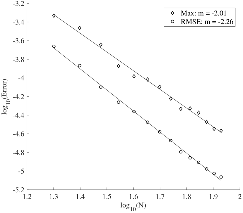
(a) Error for radii at final time.

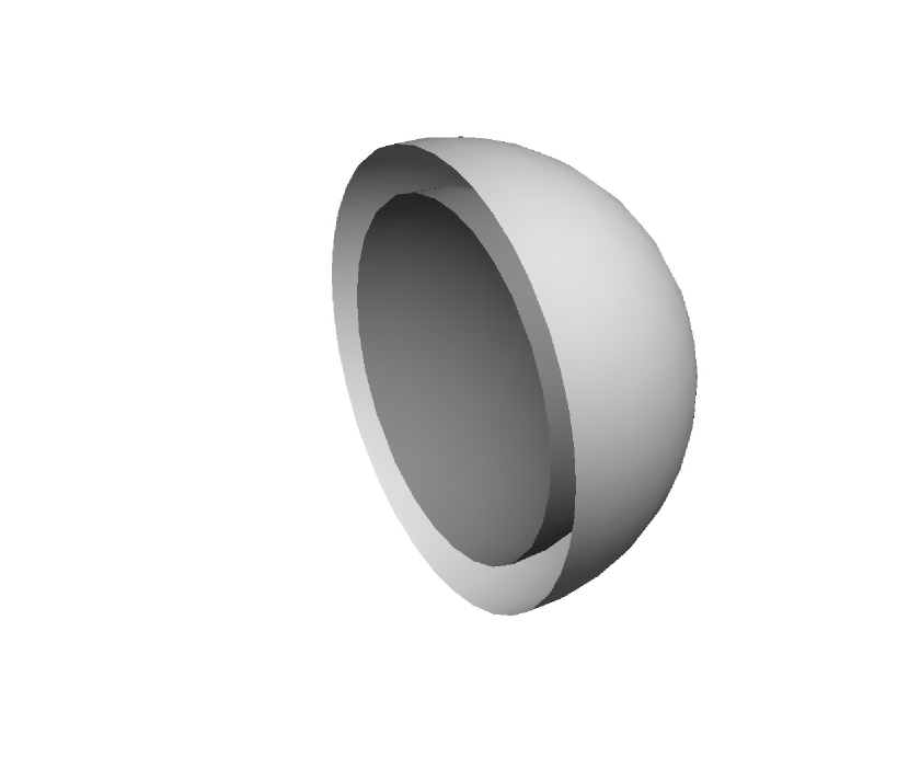
(b) Initial (inner) and final (outer) surface

Figure 14: (a) Maximum error and Root Mean Squared error (RMSE) of the radii measured at all the intersections of the surface and the grid lines. $N$ ranges from 20 to 85 with the increment $\Delta N=5$. (b) Initial surface (inner) and final surface (outer) for $N$ = 20.

4 Conclusions

In this paper, we proposed the Compact Coupling Interface Method (CCIM) to solve elliptic interface boundary value problems in any dimension. Our method combines elements from the Coupling Interface Method (CIM) and Mayo’s approach to Poisson’s equation on irregular regions. Standard central difference schemes are used at interior points. At interface points, coupling equations of the first-order derivatives and principal second-order derivatives are derived in a dimension-splitting approach by differentiating the jump conditions. Our method obtains second-order accurate solution at the grid points and second-order accurate gradient at the interface. The accurate approximation for the gradient is important in applications where the dynamics of the surface is driven by the jump of the solution gradient at the interface. Our method has more compact finite difference stencils compared with those in CIM2 and is suitable for complex interfaces. We tested our method in three dimensions with complex interfaces, including two protein surfaces, and demonstrated that the solution and the gradient at the interface are uniformly second-order accurate, and the convergence results are very robust. We also tested our method with a moving surface whose normal velocity is given by the jump in the gradient at the interface and achieved second-order accurate interface at the final time.

Statements and Declarations

Funding

This work was funded by NSF Award 1913144.

Competing Interests

The authors have no relevant financial or non-financial interests to disclose.

Data Availability

The code is available at https://github.com/Rayzhangzirui/ccim.

References

- (1) Y.C. Shu, I.L. Chern, C.C. Chang, Journal of Computational Physics 275, 642 (2014). DOI 10.1016/j.jcp.2014.07.017. URL http://www.sciencedirect.com/science/article/pii/S0021999114005105
- (2) Y. Zhong, K. Ren, R. Tsai, Journal of Computational Physics 359, 199 (2018). DOI 10.1016/j.jcp.2018.01.021. URL https://www.sciencedirect.com/science/article/pii/S0021999118300317
- (3) S. Zhou, L.T. Cheng, J. Dzubiella, B. Li, J.A. McCammon, Journal of Chemical Theory and Computation 10(4), 1454 (2014). DOI 10.1021/ct401058w. URL https://doi.org/10.1021/ct401058w
- (4) P. Macklin, J. Lowengrub, Journal of Computational Physics 203(1), 191 (2005). DOI 10.1016/j.jcp.2004.08.010. URL http://www.sciencedirect.com/science/article/pii/S0021999104003249
- (5) B. Li, SIAM Journal on Mathematical Analysis 40(6), 2536 (2009). DOI 10.1137/080712350. URL https://epubs.siam.org/doi/10.1137/080712350. Publisher: Society for Industrial and Applied Mathematics
- (6) J. Dzubiella, J.M.J. Swanson, J.A. McCammon, The Journal of Chemical Physics 124(8), 084905 (2006). DOI 10.1063/1.2171192. URL https://aip.scitation.org/doi/10.1063/1.2171192
- (7) J. Dzubiella, J.M.J. Swanson, J.A. McCammon, Physical Review Letters 96(8), 087802 (2006). DOI 10.1103/PhysRevLett.96.087802. URL https://link.aps.org/doi/10.1103/PhysRevLett.96.087802
- (8) F. Gibou, R.P. Fedkiw, L.T. Cheng, M. Kang, Journal of Computational Physics 176(1), 205 (2002). DOI 10.1006/jcph.2001.6977. URL http://www.sciencedirect.com/science/article/pii/S0021999101969773
- (9) I.L. Chern, Y.C. Shu, Journal of Computational Physics 225(2), 2138 (2007). DOI 10.1016/j.jcp.2007.03.012. URL http://www.sciencedirect.com/science/article/pii/S0021999107001246
- (10) P. Smereka, Journal of Computational Physics 211(1), 77 (2006). DOI 10.1016/j.jcp.2005.05.005. URL http://www.sciencedirect.com/science/article/pii/S0021999105002627
- (11) J. Beale, SIAM JOURNAL ON NUMERICAL ANALYSIS 42(2), 599 (2004). DOI 10.1137/S0036142903420959. Place: 3600 UNIV CITY SCIENCE CENTER, PHILADELPHIA, PA 19104-2688 USA Publisher: SIAM PUBLICATIONS Type: Article
- (12) Z. Chen, J. Zou, NUMERISCHE MATHEMATIK 79(2), 175 (1998). DOI 10.1007/s002110050336. Place: 175 FIFTH AVE, NEW YORK, NY 10010 USA Publisher: SPRINGER VERLAG Type: Article
- (13) J. Huang, J. Zou, IMA JOURNAL OF NUMERICAL ANALYSIS 22(4), 549 (2002). DOI 10.1093/imanum/22.4.549. Place: GREAT CLARENDON ST, OXFORD OX2 6DP, ENGLAND Publisher: OXFORD UNIV PRESS Type: Article
- (14) Z. Li, W. Wang, I. Chern, M. Lai, SIAM JOURNAL ON SCIENTIFIC COMPUTING 25(1), 224 (2003). DOI 10.1137/S106482750139618X. Place: 3600 UNIV CITY SCIENCE CENTER, PHILADELPHIA, PA 19104-2688 USA Publisher: SIAM PUBLICATIONS Type: Article
- (15) H. Guo, X. Yang, Journal of Computational Physics 356, 46 (2018). DOI 10.1016/j.jcp.2017.11.031. URL https://www.sciencedirect.com/science/article/pii/S0021999117308690
- (16) D. Bochkov, F. Gibou, Journal of Computational Physics 407, 109269 (2020). DOI 10.1016/j.jcp.2020.109269. URL http://www.sciencedirect.com/science/article/pii/S0021999120300437
- (17) A. Guittet, M. Lepilliez, S. Tanguy, F. Gibou, Journal of Computational Physics 298, 747 (2015). DOI 10.1016/j.jcp.2015.06.026. URL https://www.sciencedirect.com/science/article/pii/S0021999115004234
- (18) W.F. Hu, T.S. Lin, M.C. Lai. A Discontinuity Capturing Shallow Neural Network for Elliptic Interface Problems (2021). DOI 10.48550/arXiv.2106.05587. URL http://arxiv.org/abs/2106.05587. ArXiv:2106.05587 [cs, math]
- (19) H. Guo, X. Yang, Communications in Computational Physics 31(4), 1162 (2022). DOI 10.4208/cicp.OA-2021-0201. URL http://arxiv.org/abs/2107.05325. ArXiv:2107.05325 [cs, math]
- (20) S. Osher, R. Fedkiw, Level Set Methods and Dynamic Implicit Surfaces. Applied Mathematical Sciences (Springer-Verlag, New York, 2003). DOI 10.1007/b98879. URL https://www.springer.com/gp/book/9780387954820
- (21) S. Osher, J.A. Sethian, Journal of Computational Physics 79(1), 12 (1988). DOI 10.1016/0021-9991(88)90002-2. URL http://www.sciencedirect.com/science/article/pii/0021999188900022
- (22) Q. Du, X. Feng, in Handbook of Numerical Analysis, Geometric Partial Differential Equations - Part I, vol. 21, ed. by A. Bonito, R.H. Nochetto (Elsevier, 2020), pp. 425–508. DOI 10.1016/bs.hna.2019.05.001. URL https://www.sciencedirect.com/science/article/pii/S1570865919300043
- (23) A.K. Tornberg, B. Engquist, Journal of Computational Physics 200(2), 462 (2004). DOI 10.1016/j.jcp.2004.04.011. URL http://www.sciencedirect.com/science/article/pii/S0021999104001767
- (24) A.K. Tornberg, B. Engquist, Journal of Scientific Computing 19(1), 527 (2003). DOI 10.1023/A:1025332815267. URL https://doi.org/10.1023/A:1025332815267
- (25) C. Peskin, in ACTA NUMERICA 2002, VOL 11, Acta Numerica, vol. 11, ed. by A. Iserles (CAMBRIDGE UNIV PRESS, THE PITT BUILDING, TRUMPINGTON ST, CAMBRIDGE CB2 1RP, CAMBS, ENGLAND, 2002), pp. 479–517. DOI 10.1017/S0962492902000077. ISSN: 0962-4929 Type: Article
- (26) C. PESKIN, JOURNAL OF COMPUTATIONAL PHYSICS 25(3), 220 (1977). DOI 10.1016/0021-9991(77)90100-0. Place: 525 B ST, STE 1900, SAN DIEGO, CA 92101-4495 Publisher: ACADEMIC PRESS INC JNL-COMP SUBSCRIPTIONS Type: Article
- (27) R.J. LeVeque, Z. Li, SIAM Journal on Numerical Analysis 31(4), 1019 (1994). DOI 10.1137/0731054. URL https://epubs.siam.org/doi/abs/10.1137/0731054. Publisher: Society for Industrial and Applied Mathematics
- (28) Z. Li, K. Ito, SIAM Journal on Scientific Computing 23(1), 339 (2001). DOI 10.1137/S1064827500370160. URL https://epubs.siam.org/doi/abs/10.1137/S1064827500370160. Publisher: Society for Industrial and Applied Mathematics
- (29) Z. Li, SIAM Journal on Numerical Analysis 35(1), 230 (1998). DOI 10.1137/S0036142995291329. URL http://epubs.siam.org/doi/10.1137/S0036142995291329
- (30) Z. Li, H. Ji, X. Chen, SIAM Journal on Numerical Analysis 55(2), 570 (2017). DOI 10.1137/15M1040244. URL https://epubs.siam.org/doi/10.1137/15M1040244. Publisher: Society for Industrial and Applied Mathematics
- (31) X.D. Liu, T. Sideris, Mathematics of Computation 72(244), 1731 (2003). DOI 10.1090/S0025-5718-03-01525-4. URL https://www.ams.org/mcom/2003-72-244/S0025-5718-03-01525-4/
- (32) X.D. Liu, R.P. Fedkiw, M. Kang, Journal of Computational Physics 160(1), 151 (2000). DOI 10.1006/jcph.2000.6444. URL http://www.sciencedirect.com/science/article/pii/S0021999100964441
- (33) R.P. Fedkiw, T. Aslam, B. Merriman, S. Osher, Journal of Computational Physics 152(2), 457 (1999). DOI 10.1006/jcph.1999.6236. URL http://www.sciencedirect.com/science/article/pii/S0021999199962368
- (34) A. Wiegmann, K. Bube, SIAM JOURNAL ON NUMERICAL ANALYSIS 37(3), 827 (2000). DOI 10.1137/S0036142997328664. Place: 3600 UNIV CITY SCIENCE CENTER, PHILADELPHIA, PA 19104-2688 USA Publisher: SIAM PUBLICATIONS Type: Article
- (35) P. Berthelsen, JOURNAL OF COMPUTATIONAL PHYSICS 197(1), 364 (2004). DOI 10.1016/j.jcp.2003.12.003. Place: 525 B ST, STE 1900, SAN DIEGO, CA 92101-4495 USA Publisher: ACADEMIC PRESS INC ELSEVIER SCIENCE Type: Article
- (36) Y. Zhou, S. Zhao, M. Feig, G. Wei, JOURNAL OF COMPUTATIONAL PHYSICS 213(1), 1 (2006). DOI 10.1016/j.jcp.2005.07.022. Place: 525 B ST, STE 1900, SAN DIEGO, CA 92101-4495 USA Publisher: ACADEMIC PRESS INC ELSEVIER SCIENCE Type: Article
- (37) Y.C. Shu, C.Y. Kao, I.L. Chern, C.C. Chang, JOURNAL OF COMPUTATIONAL PHYSICS 229(24), 9246 (2010). DOI 10.1016/j.jcp.2010.09.001. Place: 525 B ST, STE 1900, SAN DIEGO, CA 92101-4495 USA Publisher: ACADEMIC PRESS INC ELSEVIER SCIENCE Type: Article
- (38) A. Mayo, SIAM Journal on Numerical Analysis 21(2), 285 (1984). DOI 10.1137/0721021. URL https://epubs.siam.org/doi/10.1137/0721021
- (39) W.W. Hager, SIAM Journal on Scientific and Statistical Computing 5(2), 311 (1984). DOI 10.1137/0905023. URL https://epubs.siam.org/doi/10.1137/0905023. Publisher: Society for Industrial and Applied Mathematics
- (40) R.D. Falgout, U.M. Yang, in Computational Science — ICCS 2002, ed. by P.M.A. Sloot, A.G. Hoekstra, C.J.K. Tan, J.J. Dongarra (Springer, Berlin, Heidelberg, 2002), Lecture Notes in Computer Science, pp. 632–641. DOI 10.1007/3-540-47789-6˙66
- (41) D.G. Brown, M.R. Sanderson, E. Garman, S. Neidle, Journal of Molecular Biology 226(2), 481 (1992). DOI 10.1016/0022-2836(92)90962-J. URL http://www.sciencedirect.com/science/article/pii/002228369290962J
- (42) P.H. Kussie, S. Gorina, V. Marechal, B. Elenbaas, J. Moreau, A.J. Levine, N.P. Pavletich, Science (New York, N.Y.) 274(5289), 948 (1996). DOI 10.1126/science.274.5289.948
- (43) T.J. Dolinsky, J.E. Nielsen, J.A. McCammon, N.A. Baker, Nucleic Acids Research 32(suppl_2), W665 (2004). DOI 10.1093/nar/gkh381. URL https://academic.oup.com/nar/article/32/suppl_2/W665/1040494. Publisher: Oxford Academic
- (44) J.A. Sethian, Proceedings of the National Academy of Sciences 93(4), 1591 (1996). DOI 10.1073/pnas.93.4.1591. URL http://www.pnas.org/cgi/doi/10.1073/pnas.93.4.1591