BINAS: Bilinear Interpretable
Neural Architecture Search

Abstract

Making neural networks practical often requires adhering to resource constraints such as latency, energy and memory. To solve this we introduce a Bilinear Interpretable approach for constrained Neural Architecture Search (BINAS) that is based on an accurate and simple bilinear formulation of both an accuracy estimator and the expected resource requirement, jointly with a scalable search method with theoretical guarantees. One major advantage of BINAS is providing interpretability via insights about the contribution of different design choices. For example, we find that in the examined search space, adding depth and width is more effective at deeper stages of the network and at the beginning of each resolution stage. BINAS differs from previous methods that typically use complicated accuracy predictors that make them hard to interpret, sensitive to many hyper-parameters, and thus with compromised final accuracy. Our experiments show that BINAS generates comparable to or better than state of the art architectures, while reducing the marginal search cost, as well as strictly satisfying the resource constraints.

1 Introduction

The increasing utilization of Convolutional Neural Networks (CNN) in real systems and commercial products puts neural networks with both high accuracy and fast inference speed in high demand. Early days architectures, such as VGG [38] or ResNet [14], were designed for powerful GPUs as those were the common computing platform for deep CNNs, however, in recent years the need for deployment on standard CPUs and edge devices emerged. These computing platforms are limited in their abilities and as a result require lighter architectures that comply with strict requirements on real time latency and power consumption. This has spawned a line of research aimed at finding architectures with both high performance and constrained resource demands.

The main approaches to solve this evolved from Neural Architecture Search (NAS) [46, 27, 5], while a constraint on the target latency is added over various platforms, e.g., CPU, TPU, FPGA, MCU etc. Those constrained-NAS methods can be grouped into two categories: (i) Reward based methods such as Reinforcement-Learning (RL) or Evolutionary Algorithms (EA) [4, 41, 42, 16], where the latency and accuracy of sampled architectures are predicted by evaluations on the target devices over some validation set to perform the search. The predictors are typically made of complicated models and hence require many samples and sophisticated fitting techniques [44]. Overall this oftentimes leads to inaccurate, expensive to acquire, and hard to optimize objective functions due to their complexity. (ii) Resource-aware gradient based methods formulate a differentiable loss function consisting of a trade-off between an accuracy term and either a proxy soft penalty term [18, 45] or a hard constraint [29]. Therefore, the architecture can be directly optimized via bi-level optimization using stochastic gradient descent (SGD) [2] or stochastic Frank-Wolfe (SFW) [13], respectively. However, the bi-level nature of the problem introduces many challenges [6, 26, 31, 30] and recently [43] pointed out the inconsistencies associated with using gradient information as a proxy for the quality of the architectures, especially in the presence of skip connections in the search space. These inconsistencies call for making NAS more interpretable, by extending its scope from finding optimal architectures to interpretable features [35] and their corresponding impact on the network performance.

In this paper, we propose an interpretable search algorithm that is fast and scalable, yet produces architectures with high accuracy that satisfy hard latency constraints. At the heart of our approach is an accuracy estimator which is interpretable, easy to optimize and does not have a strong reliance on gradient information. Our proposed predictor measures the performance contribution of individual design choices by sampling sub-networks from a one-shot model ([1, 7, 12, 4, 29]). Constructing the estimator this way allows making insights about the contribution of the design choices. It is important to note, that albeit its simplicity, our predictor’s performance matches that of previously proposed predictors, that are typically expensive to compute and hard to optimize due to many hyper-parameters.

The predictor we propose has a bilinear form that allows formulating the latency constrained NAS problem as an Integer Quadratic Constrained Quadratic Programming (IQCQP). Thanks to this, the optimization can be efficiently solved via a simple algorithm with some off-the-shelf components. The algorithm we suggest solves it within a few minutes on a common CPU.

Overall our optimization approach has two main performance related advantages. First, the outcome networks provide high accuracy and closely comply with the latency constraint. Second, the search is highly efficient, which makes our approach scalable to multiple target devices and latency demands.

2 Related Work

Neural Architecture Search methods automate models’ design per provided constraints. Early methods like NASNet [46] and AmoebaNet [34] focused solely on accuracy, producing SotA classification models [19] at the cost of GPU-years per search, with relatively large inference times. DARTS [27] introduced a differential space for efficient search and reduced the training duration to days, followed by XNAS [30] and ASAP [31] that applied pruning-during-search techniques to further reduce it to hours.

Predictor based methods recently have been proposed based on training a model to predict the accuracy of an architecture just from an encoding of the architecture. Popular choices for these models include Gaussian processes, neural networks, tree-based methods. See [28] for such utilization and [44] for comprehensive survey and comparisons.

Interpretabe NAS was firstly introduced by [35] through a rather elaborated Bayesian optimisation with Weisfeiler-Lehman kernel to identify beneficial topological features. We propose an intuitive and simpler approach for NAS interpretibiliy for the efficient search space examined. This leads to more understanding and applicable design rules.

Hardware-aware methods such as ProxylessNAS [5], Mnasnet [41], SPNASNet [39], FBNet [45], and TFNAS [18] generate architectures that comply to the constraints by applying simple heuristics such as soft penalties on the loss function. OFA [4] and HardCoRe-NAS [29] proposed a scalable approach across multiple devices by training an one-shot model [3, 1] once. This pretrained super-network is highly predictive for the accuracy ranking of extracted sub-networks, e.g. FairNAS [12], SPOS [12]. OFA applies evolutionary search [34] over a complicated multilayer perceptron (MLP) [36] based accuracy predictor with many hyperparameters to be tuned. HardCore-NAS searches by backpropagation [23] over a supernetwork under strict latency constraints for several GPU hours per network. Hence it requires access to a powerful GPU to perform the search and both approaches lack interpretability. This work relies on such one-shot model, for intuitively building an interpretable and simple bilinear accuracy estimator that matches in performance without any tuning and optimized under strict latency constraints by solving an IQCQP problem in several CPU minutes following by a short fine-tuning.

3 Method

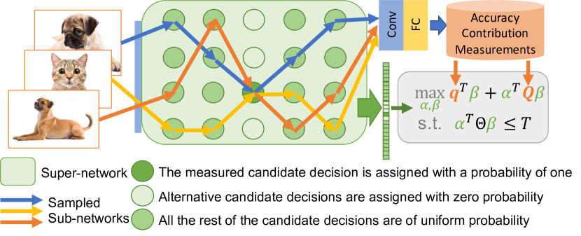
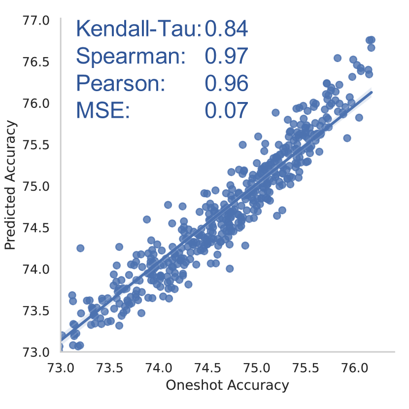
Figure 1: (Left) The BINAS scheme constructs a bilinaer accuracy estimator by measuring the accuracy contribution of individual design choices and then maximizing this objective under bilinear latency constraints. (Right) Accuracy predictions vs measured accuracy of 500 subnetworks sampled uniformly at random. High ranking correlations are achieved.

In this section we propose our method for latency-constrained NAS. We search for an architecture with the highest validation accuracy under a predefined latency constraint, denoted by $T$. We start by following [1], training a supernetwork that accommodates the search space $\mathcal{S}$, as described in section 3.1. The supernetwork training ensures that the accuracy of subnetworks extracted from it, together with their corresponding weights, are properly ranked [12, 7, 4, 29] as if those were trained from scratch. Given such a supernetwork, we sample subnetworks from it for estimating the individual accuracy contribution of each design choice (section 3.2), and construct a bilinear accuracy estimator for the expected accuracy of every possible subnetwork in the search space (section 3.3). Finally, the latency of each possible block configuration is measured on the target device and aggregated to form a bilinear latency constraint. Putting it all together (section 3.4) we formulate an IQCQP:

$$\max_{\zeta}ACC(\zeta)=q^{T}\zeta+\zeta^{T}Q\zeta$$ (1)

$$\text{s.t. }LAT(\zeta)=\zeta^{T}\Theta\zeta\leq T,\quad A_{\mathcal{S}}\cdot\zeta\leq b_{\mathcal{S}},\quad\zeta\in\mathbbm{Z}^{N}$$

where $\zeta\!=\!(\bm{\alpha},\bm{\beta})\in\mathcal{S}\!\subset\!\mathbbm{Z}^{N}$, is the parametrization of the design choices in the search space that govern the architecture structure, $q\bm{1}\in\!\mathbb{R}^{N}$, $Q\!\in\!\mathbb{R}^{N\times N}$, $\Theta\!\in\!\mathbb{R}^{N\times N}$, $A_{\mathcal{S}}\!\in\!\mathbb{R}^{C\times N}$, $b_{\mathcal{S}}\!\in\!\mathbb{R}^{C}$ and $\zeta\in\mathcal{S}$ can be expressed as a set of $C$ linear equations. Finally, in section 3.5 we propose an optimization method to efficiently solve Problem 1. Figure 1 (Left) shows a high level illustration of the scheme.

3.1 The Search Space

We consider a general search space that integrates a macro search space and a micro search space. The macro search space is composed of $S$ stages $s\in\{1,..,S\}$ of different input resolutions, each composed of blocks $b\in\{1,..,D\}$ with the same input resolution, and defines how the blocks are connected, see Figure 2. The micro search space controls the internal structures of each block. Specifically, this search space includes latency efficient search spaces introduced in [45, 16, 41, 18, 4, 29].

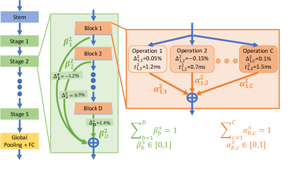
Figure 2: BINAS search space. The individual accuracy contribution and latency of each configured operation are measured.

A block configuration $c\!\in\!\mathcal{C}$ (specified in Appendix 0.B) corresponds to parameters $\bm{\alpha}$. For each block $b$ of stage $s$ we have $\alpha^{s}_{b,c}\in\{0,1\}^{\left|\mathcal{C}\right|}$ and $\Sigma_{c\in\mathcal{C}}\alpha^{s}_{b,c}=1$. An input feature map $x^{s}_{b}$ to block $b$ of stage $s$ is processed as follows: $x^{s}_{b+1}=\sum_{c\in\mathcal{C}}\alpha^{s}_{b,c}\cdot O^{s}_{b,c}(x^{s}_{b})$, where $O^{s}_{b,c}(\cdot)$ is the operation configured by $c\in\mathcal{C}$. The depth of each stage $s$ is controlled by the parameters $\bm{\beta}$: $x^{s+1}_{1}=\Sigma_{b=1}^{D}\beta^{s}_{b}\cdot x^{s}_{b+1}$, such that $\beta^{s}_{b}\in\{0,1\}^{D}$ and $\Sigma_{b=1}^{D}\beta^{s}_{b}=1$.

To summarize, the search space is composed of both the micro and macro search spaces parameterized by $\bm{\alpha}$ and $\bm{\beta}$, respectively:

$$\mathcal{S}=\left\{(\bm{\alpha},\bm{\beta})\left|\begin{array}[]{c}\alpha^{s}_{b,c}\in\{0,1\}^{\left|\mathcal{C}\right|}\,;\,\Sigma_{c\in\mathcal{C}}\alpha^{s}_{b,c}=1\\ \beta^{s}_{b}\in\{0,1\}^{D}\,;\,\Sigma_{b=1}^{D}\beta^{s}_{b}=1\\ \end{array}\right.;\begin{array}[]{l}\forall s\in\{1,..,S\}\\ \forall b\in\{1,..,D\},c\in\mathcal{C}\end{array}\right\}$$ (6)

such that a continuous probability distribution is induced over the space, by relaxing $\alpha^{s}_{b,c}\in\{0,1\}^{\left|\mathcal{C}\right|}$ to $\alpha^{s}_{b,c}\in\mathbb{R}_{+}^{\left|\mathcal{C}\right|}$ and $\beta^{s}_{b}\in\{0,1\}^{D}$ to $\beta^{s}_{b}\in\mathbb{R}_{+}^{D}$ to be continuous rather than discrete. Therefore, this probability distribution can be expressed by a set of linear equations and one can view the parametrization $\zeta=(\bm{\alpha},\bm{\beta})$ as a composition of probabilities in $\mathcal{P}_{\zeta}(\mathcal{S})=\{\zeta\mid A_{\mathcal{S}}\zeta\leq b_{\mathcal{S}}\}=\{(\bm{\alpha},\bm{\beta})\mid A_{\mathcal{S}}^{\alpha}\cdot\bm{\alpha}\leq b_{\mathcal{S}}^{\alpha},A_{\mathcal{S}}^{\beta}\cdot\bm{\beta}\leq b_{\mathcal{S}}^{\beta}\}$ or as degenerate one-hot vectors in $\mathcal{S}$.

3.2 Estimating the Accuracy Contribution of Design Choices

Next we introduce a simple way to estimate the accuracy contribution of each design choice, given a trained one-shot model. With this at hand, we will be able to select those design choices that contribute the most to the accuracy under some latency budget. Suppose a supernetwork is constructed, such that every sub-network of it resides in the search space of Section 3.1. The supernetwork is trained to rank well different subnetworks [12, 7, 4, 29]. The expected accuracy of such a supernetwork $\mathbb{E}[Acc]$ is estimated by uniformly sampling a different subnetwork for each input image from 20% of the Imagenet train set (considered as a validation set), as illustrated in Figure 3.

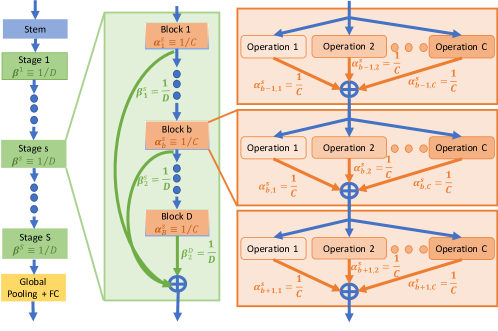
Figure 3: Estimating the base accuracy of the supernetwork is done by random uniform sampling of subnetworks for each input image.

This estimate serves as the base accuracy of the supernetwork and thus every design choice should be evaluated by its contribution on top of it. Hence, the individual accuracy contribution of setting the depth of stage $s$ to $b$ is the gap: $\Delta_{b}^{s}=\mathbb{E}[Acc|d^{s}=b]-\mathbb{E}[Acc]$, where the first expectation is estimated by setting $\beta^{s}_{b}=1$ and uniform distribution for the rest of the design choices. This is done for every possible depth of every stage (Figure 4).

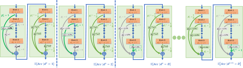
Figure 4: Estimating the expected accuracy gap caused by macroscopic design choices of the depth of the stages.

Similarly, the individual accuracy contribution of choosing configuration $c$ in block $b$ of stage $s$ is given by the gap: $\Delta_{b,c}^{s}=\mathbb{E}[Acc|O_{b,c}^{s}=O_{c},d^{s}=b]-\mathbb{E}[Acc]$, where the first expectation is estimated by setting $\alpha_{b,c}^{s}=1$ and $\beta^{s}_{b}=1$, while keeping a uniform distribution for all the rest of the design choices in the supernetwork, as illustrated in Figure 5.

Figure 5: Estimating the expected accuracy gap caused by microscopic design choices on the operation applied at every block one at a time.

3.3 Constructing a Bilnear Accuracy Estimator

We next propose an intuitive and effective way to utilize the estimated individual accuracy contribution of each design choice (section 3.2) to estimate the expected overall accuracy of a certain architecture in the search space.

The expected accuracy contribution of a block $b$ can be computed by summing over the accuracy contributions $\Delta^{s}_{b,c}$ of every possible configuration $c\in\mathcal{C}$: $\bar{\delta}^{s}_{b}=\Sigma_{c\in\mathcal{C}}\alpha^{s}_{b,c}\cdot\Delta^{s}_{b,c}$ Thus the expected accuracy contribution of the stage $s$ of depth $b^{\prime}$ is $\delta^{s}_{b^{\prime}}=\Delta^{s}_{b^{\prime}}+\Sigma_{b=1}^{b^{\prime}}\bar{\delta}^{s}_{b}$, where the first term is the accuracy contribution associated solely with the choice of depth $b^{\prime}$ and the second term is the aggregation of the expected accuracy contributions of the first $b^{\prime}$ blocks in the stage. Taking the expectation over all possible depths for stage $s$ yields $\delta^{s}=\sum_{b^{\prime}=1}^{D}\beta^{s}_{b^{\prime}}\cdot\delta^{s}_{b^{\prime}}$ and summing over all the stages results in the aggregated accuracy contribution of all design choices. Hence the accuracy of a subnetwork can be calculated by this estimated contribution on top of the estimated base accuracy $\mathbb{E}[Acc]$ (Figure 3):

$$ACC(\bm{\alpha},\bm{\beta})=\mathbb{E}[Acc] +\sum_{s=1}^{S}\sum_{b=1}^{D}\beta^{s}_{b}\cdot\Delta_{b}^{s}+\sum_{s=1}^{S}\sum_{b=1}^{D}\sum_{b^{\prime}=b}^{D}\sum_{c\in\mathcal{C}}\alpha^{s}_{b,c}\cdot\Delta_{b,c}^{s}\cdot\beta^{s}_{b^{\prime}}$$ (7)

And its vectorized form can be expressed as the following bilinear formula in $\bm{\alpha}$ and $\bm{\beta}$: $ACC(\bm{\alpha},\bm{\beta})=r+q_{\beta}^{T}\bm{\beta}+\bm{\alpha}^{T}Q_{\alpha\beta}\bm{\beta}$, where $r=E[Acc]$, $q_{\beta}\in\mathbb{R}^{D\cdot S}$ is a vector composed of $\Delta_{b}^{s}$ and $Q_{\alpha\beta}\in\mathbb{R}^{\mathcal{C}\cdot D\cdot S\times D\cdot S}$ is a matrix composed of $\Delta_{b,c}^{s}$.

We next present a theorem (with proof in Appendix 0.D) that states that the estimator in equation 7 approximates well the expected accuracy of an architecture.

Theorem 3.1

Assume $\{O^{s}_{b},d_{s}\}$ for $s=1,\dots,S$ and $b=1,\dots,D$ are conditionally independent with the accuracy $Acc$. Suppose that there exists a positive real number $0<\epsilon\ll 1$ such that for any $X\in\{O^{s}_{b},d_{s}\}$ the following holds $|\mathbb{P}[Acc|X]-\mathbb{P}[Acc]|<\epsilon\mathbb{P}[Acc]$. Then:

$$\mathbb{E}\left[Acc\middle|\cap_{s=1}^{S}\cap_{b=1}^{D}O^{s}_{b},\cap_{s=1}^{S}d^{s}\right] =\mathbb{E}[Acc]+\left(1+\mathcal{O}(N\epsilon)\right)\cdot\sum_{s=1}^{S}\sum_{b=1}^{D}\beta^{s}_{b}\cdot\Delta_{b}^{s}$$ (8)

$$+\left(1+\mathcal{O}(N\epsilon)\right)\cdot\sum_{s=1}^{S}\sum_{b=1}^{D}\sum_{b^{\prime}=b}^{D}\sum_{c\in\mathcal{C}}\alpha^{s}_{b,c}\cdot\Delta_{b,c}^{s}\cdot\beta^{s}_{b^{\prime}}$$

Theorem 3.1 and Figure 1 (right) demonstrate the effectiveness of relying on $\Delta_{b,c}^{s}$, $\Delta_{b}^{s}$ to express the expected accuracy of networks. Since those terms measure the accuracy contributions of individual design decisions, many insights and design rules can be extracted from those, as discussed in section 5.3, making the proposed estimator intuitively interpretable. Furthermore, the transitivity of ranking correlations is used in appendix 0.H for guaranteeing good prediction performance with respect to architectures trained from scratch.

3.4 The Interger Quadratic Constraints Quadratic Program

In this section we formulate latency-constrained NAS as an IQCQP of bilinear objective function and bilinear constraints. For the purpose of maximizing the validation accuracy of the selected subnetwork under latency constraint, we utilize the bilinear accuracy estimator derived in section 3.3 as the objective function and define the bilinear latency constraint similarly to  [18, 29]:

$$LAT(\bm{\alpha},\bm{\beta})=\sum_{s=1}^{S}\sum_{b=1}^{D}\sum_{b^{\prime}=b}^{D}\sum_{c\in\mathcal{C}}\alpha^{s}_{b,c}\cdot t^{s}_{b,c}\cdot\beta^{s}_{b^{\prime}}=\bm{\alpha}^{T}\Theta\bm{\beta}$$ (9)

where $\Theta\in\mathbb{R}^{\mathcal{C}\cdot D\cdot S\times D\cdot S}$ is a matrix composed of the latency measurements $t^{s}_{b,c}$ on the target device of each configuration $c\in\mathcal{C}$ of every block $b$ in every stage $s$ (Figure 2). The bilinear version of problem 1 turns to be:

$$\max_{\alpha^{s}_{b,c},\beta^{s}_{b}} \sum_{s=1}^{S}\sum_{b=1}^{D}\beta^{s}_{b}\cdot\Delta_{b}^{s}+\sum_{s=1}^{S}\sum_{b=1}^{D}\sum_{b^{\prime}=b}^{D}\sum_{c\in\mathcal{C}}\alpha^{s}_{b,c}\cdot\Delta_{b,c}^{s}\cdot\beta^{s}_{b^{\prime}}$$ (10)

s.t. $$\sum_{s=1}^{S}\sum_{b=1}^{D}\sum_{b^{\prime}=b}^{D}\sum_{c\in\mathcal{C}}\alpha^{s}_{b,c}\cdot t^{s}_{b,c}\cdot\beta^{s}_{b^{\prime}}\leq T$$

$$\Sigma_{c\in\mathcal{C}}\alpha^{s}_{b,c}=1\,;\,\alpha^{s}_{b,c}\in\{0,1\}^{\left|\mathcal{C}\right|}\,\,\forall s\in\{1,..,S\},b\in\{1,..,D\},c\in\mathcal{C}$$

$$\Sigma_{b=1}^{D}\beta^{s}_{b}=1\,;\,\beta^{s}_{b}\in\{0,1\}^{D}\,\,\forall s\in\{1,..,S\},b\in\{1,..,D\}$$

And in its vectorized form:

$$\max_{\bm{\alpha},\bm{\beta}\in\{0,1\}}q_{\beta}^{T}\bm{\beta}+\bm{\alpha}^{T}Q_{\alpha\beta}\bm{\beta}\text{ s.t. }\bm{\alpha}^{T}\Theta\bm{\beta}\leq T\,;\,A_{\mathcal{S}}^{\alpha}\cdot\bm{\alpha}\leq b_{\mathcal{S}}^{\alpha}\,;\,A_{\mathcal{S}}^{\beta}\cdot\bm{\beta}\leq b_{\mathcal{S}}^{\beta}$$ (11)

3.5 Solving the Integer Quadratic Constraints Quadratic Program

By formulating the latency-constrained NAS as a binary problem in section 3.4, we can now use out-of-the-box Mixed Integer Quadratic Constraints Programming (MIQCP) solvers to optimize problem 10. We use IBM CPLEX [20] that supports non-convex binary QCQP and utilizes the Branch-and-Cut algorithm [32] for this purpose. A heuristic alternative for optimizing an objective function under integer constraints is evolutionary search [34]. Next we propose a more theoretically sound alternative.

3.5.1 Utilizing the Block Coordinate Frank-Wolfe Algorithm

As pointed out by [29], since $\Theta$ is constructed from measured latency in equation 9, it is not guaranteed to be positive semi-definite, hence, the induced quadratic constraint makes the feasible domain in problem 1 non-convex in general. To overcome this we adapt the Block-Coordinate Frank-Wolfe (BCFW) [24] for solving a continuous relaxation of problem 1, such that $\zeta\in\mathbb{R}_{+}^{N}$. Essentially BCFW adopts the Frank-Wolfe [10] update rule for each block of coordinates in $\delta\in\{\bm{\alpha},\bm{\beta}\}$ picked up at random at each iteration $k$, such that $\delta_{k+1}=(1-\gamma_{k})\cdot\delta_{k}+\gamma_{k}\cdot\hat{\delta}$ with $0\leq\gamma_{k}\leq 1$, for any partially differentiable objective function $ACC(\bm{\alpha},\bm{\beta})$:

$$\hat{\bm{\alpha}}= \operatornamewithlimits{argmax~{}}_{\bm{\alpha}}\nabla_{\bm{\alpha}}ACC(\bm{\alpha},\bm{\beta}_{k})^{T}\cdot\bm{\alpha}\quad\text{ s.t. }\bm{\beta}_{k}^{T}\Theta^{T}\cdot\bm{\alpha}\leq T\quad;\quad A_{\mathcal{S}}^{\alpha}\cdot\bm{\alpha}\leq b_{\mathcal{S}}^{\alpha}$$ (12)

$$\hat{\bm{\beta}}= \operatornamewithlimits{argmax~{}}_{\bm{\beta}}\nabla_{\bm{\beta}}ACC(\bm{\alpha}_{k},\bm{\beta})^{T}\cdot\bm{\beta}\quad\text{ s.t. }\bm{\alpha}_{k}^{T}\Theta\cdot\bm{\beta}\leq T\quad;\quad A_{\mathcal{S}}^{\beta}\cdot\bm{\beta}\leq b_{\mathcal{S}}^{\beta}$$ (13)

where $\nabla_{\delta}$ stands for the partial derivatives with respect to $\delta$. Convergence guarantees are provided in [24]. Then, once converged to the solution of the continuous relaxation of the problem, we need to project the solution back to the discrete space of architectures, specified in equation 6, as done in [29]. This step could deviate from the solution and cause degradation in performance.

Due to the formulation of the NAS problem 11 as a Bilinear Programming (BLP) [11] with bilinear constraints (BLCP) we design Algorithm 1 that applies the BCFW with line-search for this special case. Thus more specific convergence guarantees can be provided together with the sparsity of the solution, hence no additional discretization step is required. The following theorem states that after $\mathcal{O}(1/\epsilon)$ iterations, Algorithm 1 obtains an $\epsilon$-approximate solution to problem 11.

Algorithm 1 BCFW with Line Search for BLCP

0:  $(\bm{\alpha}_{0},\bm{\beta}_{0})\in\left\{(\bm{\alpha},\bm{\beta})\left|\begin{array}[]{c}\bm{\alpha}^{T}\Theta\bm{\beta}\leq T,A_{\mathcal{S}}^{\alpha}\bm{\alpha}\leq b_{\mathcal{S}}^{\alpha},A_{\mathcal{S}}^{\beta}\bm{\beta}\leq b_{\mathcal{S}}^{\beta}\end{array}\right.\right\}$

1:  for $k=0,\dots,K-1$ do

2:     if $Bernoulli(p)==1$ then

3:        $\bm{\alpha}_{k+1}=\operatornamewithlimits{argmax~{}}_{\bm{\alpha}}(q^{T}_{\alpha}+\beta_{k}^{T}Q_{\alpha\beta}^{T})\cdot\bm{\alpha}$ s.t. $\bm{\beta}_{k}^{T}\Theta^{T}\cdot\bm{\alpha}\leq T$ ; $A_{\mathcal{S}}^{\alpha}\cdot\bm{\alpha}\leq b_{\mathcal{S}}^{\alpha}$ and $\bm{\beta}_{k+1}=\bm{\beta}_{k}$

4:     else

5:        $\bm{\beta}_{k+1}=\operatornamewithlimits{argmax~{}}_{\bm{\beta}}(q^{T}_{\beta}+\alpha_{k}^{T}Q_{\alpha\beta})\cdot\bm{\beta}$ s.t. $\bm{\alpha}_{k}^{T}\Theta\cdot\bm{\beta}\leq T$ ; $A_{\mathcal{S}}^{\beta}\cdot\bm{\beta}\leq b_{\mathcal{S}}^{\beta}$ and $\bm{\alpha}_{k+1}=\bm{\alpha}_{k}$

6:     end if

7:  end for

7:  $\zeta^{*}=(\bm{\alpha}_{K},\bm{\beta}_{K})$

Theorem 3.2

For each $k>0$ the iterate $\zeta_{k}=(\bm{\alpha}_{k},\bm{\beta}_{k})$ of Algorithm 1 satisfies:

$$E[ACC(\zeta_{k})]-ACC(\zeta^{*})\leq\frac{4}{k+4}\left(ACC(\zeta_{0})-ACC(\zeta^{*})\right)$$

where $\zeta^{*}=(\bm{\alpha}^{*},\bm{\beta}^{*})$ is the solution of a continuous relaxation of problem 11 and the expectation is over the random choice of the block $\bm{\alpha}$ or $\bm{\beta}$.

The proof is in Appendix 0.F. We next provide a guarantee that Algorithm 1 directly yields a sparse solution, representing a valid sub-network without the additional discretization step required by other continuous methods [27, 45, 18, 29].

Theorem 3.3

The output solution $(\bm{\alpha},\bm{\beta})=\zeta^{*}$ of Algorithm 1 contains only one-hot vectors for $\alpha^{s}_{b,c}$ and $\beta^{s}_{b}$, except from a single one for each of those blocks, which contains a couple of non-zero entries.

The proof is in Appendix 0.G. In practice, a negligible latency deviation is associated with taking the $\operatornamewithlimits{argmax~{}}$ over the only two couples. Differently from the sparsity guarantee for the discretization step in [29], Theorem 3.3 guarantees similar desirable properties but for the fundamentally different Algorithm 1 that does not involve an additional designated projection step.

4 Experimental Results

Figure 6: Imagenet Top-1 accuracy vs latency. All models are trained from scratch. BINAS generates better models than other methods with a reduced scalable marginal cost of 8 GPU hours for each additional model.

4.1 Search for State-of-the-Art Architectures

4.1.1 Search Space Specifications.

Aiming at latency efficient architectures, we adopt the search space introduced in [29], which is closely related to those used by [45, 16, 41, 18, 4]. The macro search space is composed of $S=5$ stages, each composed of at most $D=4$ blocks. The micro search space is based on Mobilenet Inverted Residual (MBInvRes) blocks [37] and controls the internal structures of each block. Every MBInvRes block is configured by an expansion ratio $er\in\{3,4,6\}$ of the point-wise convolution, kernel size $k\in\{3\times 3,5\times 5\}$ of the Depth-Wise Separable convolution (DWS), and Squeeze-and-Excitation (SE) layer [17] $se\in\{\text{on},\text{off}\}$ (details in Appendix 0.B).

4.1.2 Comparisons with Other Methods.

We compare our generated architectures to other state-of-the-art NAS methods in Table 1 and Figures 6 and 7 (Right). Aiming for surpassing the previous state-of-the-art [29] search methods, we use its search space (Section 4.1.1) and official supernetwork training. This way we can show that the improved search method (Section 5.4 and Figure 7 (Middle)) leads to superior results for the same marginal search cost of 15 GPU hours per additional generated model, as shown in Figure 7 (Right). For the purpose of comparing the generated architectures alone of other methods, excluding the contribution of evolved pretraining techniques, for each model in Table 1 and Figure  7 (Right), the official PyTorch implementation [33] is trained from a scratch using the exact same code and hyperparameters, as specified in appendix 0.C. The maximum accuracy between our training and the original paper is reported. The latency values presented are actual time measurements of the models, running on a single thread with the exact same settings and on the same hardware. We disabled optimizations, e.g., Intel MKL-DNN [21], hence the latency we report may differ from the one originally reported. It can be seen that networks generated by our method meet the latency target closely, while at the same time are comparable to or surpassing all the other methods on the top-1 Imagenet accuracy with a reduced scalable search cost. The total search time consists of $435$ GPU hours computed only once as preprocessing and additional $8$ GPU hours for fine-tuning each generated network, while the search itself requires negligible several CPU minutes, see appendix 0.A for more details. Due to the negligible search cost, one can choose to train the models longer (e.g. 15 GPU hours) to achieve better results with no larger marginal cost than other methods.

Model Latency (ms) Top-1 (%) Total Cost (GPU hours) MnasNetB1 39 74.5 40,000N TFNAS-B 40 75.0 263N SPNASNet 41 74.9 288 + 408N OFA CPU 42 75.7 1200 + 25N HardCoRe A 40 75.8 400 + 15N BINAS(40) 40 76.1 435 + 8N BINAS∗(40) 40 76.5 435 + 15N MobileNetV3 45 75.2 180N FBNet 47 75.7 576N MnasNetA1 55 75.2 40,000N HardCoRe B 44 76.4 400 + 15N BINAS(45) 45 76.5 435 + 8N BINAS∗(45) 45 77.0 435 + 15 MobileNetV2 70 76.5 150N TFNAS-A 60 76.5 263N HardCoRe C 50 77.1 400 + 15N BINAS(50) 50 76.8 435 + 8N BINAS∗(50) 50 77.6 435 + 15N EfficientNetB0 85 77.3 HardCoRe D 55 77.6 400 + 15N BINAS(55) 55 77.7 435 + 8N BINAS∗(55) 55 77.8 435 + 15N FairNAS-C 60 77.0 240N HardCoRe E 61 78.0 400 + 15N BINAS(60) 59 77.8 435 + 8N BINAS∗(60) 59 78.0 435 + 15N

Model Latency (ms) Top-1 (%) MobileNetV3 28 75.2 TFNAS-D 30 74.2 HardCoRe A 27 75.7 BINAS(25) 26 76.1 BINAS∗(25) 26 76.6 MnasNetA1 37 75.2 MnasNetB1 34 74.5 FBNet 41 75.7 SPNASNet 36 74.9 TFNAS-B 44 76.3 TFNAS-C 37 75.2 HardCoRe B 32 77.3 BINAS(30) 31 76.8 BINAS∗(30) 31 77.2 TFNAS-A 54 76.9 EfficientNetB0 48 77.3 MobileNetV2 50 76.5 HardCoRe C 41 77.9 BINAS(40) 40 77.6 BINAS∗(40) 40 77.7

Table 1: ImageNet top-1 accuracy, latency and cost comparison with other methods. The total cost stands for the search and training cost of N networks. Latency is reported for (Left) Intel Xeon CPU and (Right) NVIDIA P100 GPU with a batch size of 1 and 64 respectively.

5 Empirical Analysis of Key Components

In this section we analyze and discuss different aspects of the proposed method.

5.1 The Contribution of Different Terms of the Accuracy Estimator

Variant	Kendall-Tau	Spearman
$q_{\beta}\equiv 0$	0.29	0.42
$Q_{\alpha\beta}\equiv 0$	0.66	0.85
$ACC(\bm{\alpha},\bm{\beta})$	0.84	0.97

Table 2: Contribution of terms.

The accuracy estimator in equation 7 aggregates the contributions of multiple architectural decisions. In section 3.3, those decisions are grouped into two groups: (1) macroscopic decisions about the depth of each stage are expressed by $q_{\beta}$ and (2) microscopic decisions about the configuration of each block are expressed by $Q_{\alpha\beta}$. Table 2 quantifies the contribution of each of those terms to the ranking correlations by setting the corresponding terms to zero. We conclude that the depth of the network is very significant for estimating the accuracy of architectures, as setting $q_{\beta}$ to zero specifically decreases the Kendall-Tau and Spearman’s correlation coefficients from $0.84$ and $0.97$ to $0.29$ and $0.42$ respectively. The significance of microscopic decisions about the configuration of blocks is also viable but not as much, as setting $Q_{\alpha\beta}$ to zero decreases the Kendall-Tau and Spearman’s correlation to $0.66$ and $0.85$ respectively.

5.2 Comparison to Learning the Accuracy Predictors

While the purpose of this work is not to compare many accuracy predictors, as this has been already done comprehensively by [44], comparisons to certain learnt predictors support the validity and benefits of the proposed accuracy estimator (section 3.3) despite its simple functional form. Hence each of the following comparisons is chosen for a reason: (1) Showing that it is more sample efficient than learning the parameters of a bilinear predictor of the same functional form. (2) Comparing to a quadratic predictor shows that reducing the functional form to bilinear by omitting the interactions between microscopic decisions ($\bm{\alpha}$ parameters) to each other and of macroscopic decisions ($\bm{\beta}$ parameters) to each other does not cause much degradation. (3) Comparing to a parameter heavy MLP predictor shows that the simple bilinear parametric form does not lack the expressive power required for properly ranking architectures.

5.2.1 Learning Quadratic Accuracy Predictors

One can wonder whether setting the coefficients $Q_{\alpha\beta}$, $q_{\beta}$ and $r$ of the bilinear form in section 3.3 according to the estimates in section 3.2 yields the best predictions of the accuracy of architectures. An alternative approach is to learn those coefficients by solving a linear regression:

$$\min_{\tilde{r},\tilde{q}_{\alpha},\tilde{q}_{\beta},\tilde{Q}_{\alpha\beta}}\sum_{i=1}^{n}||\mathcal{B}_{\tilde{r},\tilde{q}_{\alpha},\tilde{q}_{\beta},\tilde{Q}_{\alpha\beta}}(\bm{\alpha}_{i},\bm{\beta}_{i})-Acc(\bm{\alpha}_{i},\bm{\beta}_{i})||_{2}^{2}$$ (14)

$$\mathcal{B}_{\tilde{r},\tilde{q}_{\alpha},\tilde{q}_{\beta},\tilde{Q}_{\alpha\beta}}(\bm{\alpha}_{i},\beta_{i})=\tilde{r}+\bm{\alpha}_{i}^{T}\tilde{q}_{\alpha}+\bm{\beta}_{i}^{T}\tilde{q}_{\beta}+\bm{\alpha}_{i}^{T}\tilde{Q}_{\alpha\beta}\bm{\beta}_{i}$$ (15)

where $\{\bm{\alpha}_{i},\bm{\beta}_{i}\}_{i=1}^{n}$ and $Acc(\bm{\alpha}_{i},\bm{\beta}_{i})$ represent $n$ uniformly sampled subnetworks and their measured accuracy, respectively.

One can further unlock the full capacity of a quadratic predictor by coupling of all components and solving the following linear regression problem:

$$\min_{\tilde{r},\tilde{q}_{\alpha},\tilde{q}_{\beta},\tilde{Q}_{\alpha\beta},\tilde{Q}_{\alpha},\tilde{Q}_{\beta}}\sum_{i=1}^{n}||\mathcal{Q}_{\tilde{r},\tilde{q}_{\alpha},\tilde{q}_{\beta},\tilde{Q}_{\alpha\beta},\tilde{Q}_{\alpha},\tilde{Q}_{\beta}} (\bm{\alpha}_{i},\bm{\beta}_{i})-Acc(\bm{\alpha}_{i},\bm{\beta}_{i})||_{2}^{2}$$

$$\mathcal{Q}_{\tilde{r},\tilde{q}_{\alpha},\tilde{q}_{\beta},\tilde{Q}_{\alpha\beta},\tilde{Q}_{\alpha},\tilde{Q}_{\beta}}(\bm{\alpha}_{i},\bm{\beta}_{i})=\mathcal{B}_{\tilde{r},\tilde{q}_{\alpha},\tilde{q}_{\beta},\tilde{Q}_{\alpha\beta}}(\bm{\alpha}_{i},\beta_{i})+\bm{\alpha}_{i}^{T}\tilde{Q}_{\alpha}\bm{\alpha}_{i}+\bm{\beta}_{i}^{T}\tilde{Q}_{\beta}\bm{\beta}_{i}$$ (16)

A closed form solution to these problems is derived in appendix 0.E. While effective, this solution requires avoiding memory issues associated with inverting $N^{2}\times N^{2}$ matrix and also reducing overfitting by tuning regularization effects over train-val splits of the data points. The data points for training all the accuracy predictors is composed of subnetworks uniformly sampled from the supernetwork and their corresponding validation accuracy is measured over the same 20% of the Imagenet train set split used in section 3.2.

Figure 7 (Left) presents the Kendall-Tau ranking correlation coefficients and mean square error (MSE), measured over 500 test data points generated uniformly at random in the same way, of different accuracy predictors versus the number of data points corresponding to the number of epochs of the validation set required for obtaining their parameters. It is noticable that the simple bilinear accuracy estimator (section 3.3) is more sample efficient, as its parameters are efficiently estimated according to section 3.2 rather than learned.

5.2.2 Beyond Quadratic Accuracy Predictors

The reader might question the expressiveness of a simple bilinear parametric form and its ability to capture the complexity of architectures. To alleviate such concerns we show in Figure 7 (Left) that the proposed bilinear estimator of section 3.3 matches the performance of the commonly used parameters heavy Multi-Layer-Perceptron (MLP) accuracy predictor [4, 28]. Moreover, the MLP predictor is more complex and requires extensive hyperparameter tuning, e.g., of the depth, width, learning rate and its scheduling, weight decay, optimizer etc. It is also less efficient, lacks interpretability, and of limited utility as an objective function for NAS (Section 3.5).

Figure 7: (Left) Performance of predictors vs samples. Ours is comparable to complex alternatives and sample efficient. (Middle) Comparing optimizers for solving the IQCQP over 5 seeds. All surpass optimizing the supernetwork (HardCoreNAS) directly. (Right) Surpassing State-of-the-Art. BINAS generates superior models than HardCoReNAS for the same search space, supernetwork weights and marginal cost of 15 GPU hours.

5.3 Interpretability of the Accuracy Estimator

Given that the accuracy estimator in section 3.3 ranks architectures well, as demonstrated in Figure 1 (Right), this accountability together with the way it is constructed bring insights about the contribution of different design choices to the accuracy, as shown in Figure 8.
Deepen later stages: In the left figure $\Delta_{b}^{s}-\Delta_{b-1}^{s}$ are presented for $b=3,4$ and $s=1,\dots,5$. This graph shows that increasing the depth of deeper stages is more beneficial than doing so for shallower stages. Showing also the latency cost for adding a block to each stage, we see that there is a strong motivation to make later stages deeper.
Add width and S&E to later stages and shallower blocks: In the middle and right figures, $\Delta_{b,c}^{s}$ are averaged over different configurations and blocks or stages respectively for showing the contribution of microscopic design choices. Those show that increasing the expansion ratio and adding S&E are more significant in deeper stages and at sooner blocks within each stage.
Prefer width and S&E over bigger kernels: Increasing the kernel size is relatively less significant and is more effective at intermediate stages.

Figure 8: Design choices insights deduced from the accuracy estimator: The contribution of (Left) depth for different stages, (Middle) expansion ration, kernel size and S&E for different stages and (Right) for different blocks within a stage.

5.4 Comparison of Optimization Algorithms

Formulating the NAS problem as IQCQP affords the utilization of a variety of optimization algorithms. Figure 7 (Middle) compares the one-shot accuracy and latency of networks generated by utilizing the algorithms suggested in section 3.5 for solving problem 1 with the bilinear estimator introduced in section 3.3 serving as the objective function. Error bars for both accuracy and latency are presented for 5 different seeds. All algorithms satisfy the latency constraints up to a reasonable error of less than $10\%$. While all of them surpass the performance of BCSFW [29], given as reference, BCFW is superior at low latency, evolutionary search does well over all and MIQCP is superior at high latency. Hence, for practical purposes we apply the three of them for search and take the best one, with negligible computational cost of less than three CPU minutes overall.

6 Conclusion

The problem of resource-aware NAS is formulated as an IQCQP optimization problem. Bilinear constraints express resource requirements and a bilinear accuracy estimator serves as the objective function. This estimator is constructed by measuring the individual contribution of design choices, which makes it intuitive and interpretable. Indeed, its interpretability brings several insights and design rules. Its performance is comparable to complex predictors that are more expensive to acquire and harder to optimize. Efficient optimization algorithms are proposed for solving the resulted IQCQP problem. BINAS is a faster search method, scalable to many devices and requirements, while generating comparable or better architectures than those of other state-of-the-art NAS methods.

Appendix

Appendix 0.A An Overview of the Method and Computational Costs

Figure 9 presents and overview scheme of the method:

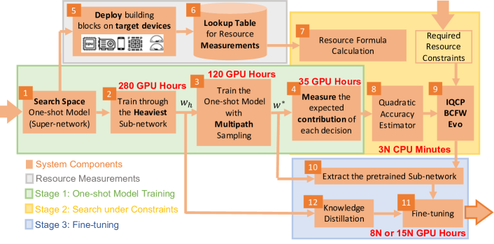
Figure 9: An Overview scheme of the IQNAS method with computational costs

The search space, latency measurements and formula, supernetwork training and fine-tuning blocks (1,2,3,5,6,7,10,11,12) are identical to those introduced in HardCoRe-NAS:

We first train for 250 epochs a one-shot model $w_{h}$ using the heaviest possible configuration, i.e., a depth of $4$ for all stages, with $er=6,k=5\times 5,se=on$ for all the blocks. Next, to obtain $w^{*}$, for additional 100 epochs of fine-tuning $w_{h}$ over 80% of a 80-20 random split of the ImageNet train set [9]. The training settings are specified in appendix 0.C. The first 250 epochs took 280 GPU hours and the additional 100 fine-tuning epochs took 120 GPU hours, both Running with a batch size of 200 on 8$\times$NVIDIA V100, summing to a total of 400 hours on NVIDIA V100 GPU to obtain both $w_{h}$ and $w^{*}$.

A significant benefit of this training scheme is that it also shortens the generation of trained models. The common approach of most NAS methods is to re-train the extracted sub-networks from scratch. Instead, we follow HardCoRe-NAS and leverage having two sets of weights: $w_{h}$ and $w^{*}$. Instead of retraining the generated sub-networks from a random initialization we opt for fine-tuning $w^{*}$ guided by knowledge distillation [15] from the heaviest model $w_{h}$. Empirically, as shown in figure 6 by comparing the dashed red line with the solid one, we observe that this surpasses the accuracy obtained when training from scratch at a fraction of the time: 8 GPU hours for each generated network.

The key differences from HardCoRe-NAS reside in the latency constrained search blocks (4,8,9 of figure 9) that have to do with constructing the quadratic accuracy estimator of section 3.3 and solving the IQCQP problem. The later requires only several minutes on CPU for each generated netowork (compared to 7 GPU hours of HardCoRe-NAS), while the former requires to measure the individual accuracy contribution of each decision. Running a validation epoch to estimate $\mathbb{E}[Acc]$ and also for each decision out of all $255$ entries in the vector $\zeta$ to obtain $\Delta_{b,c}^{s}$ and $\Delta_{b}^{s}$ requires 256 validation epochs in total that last for 3.5 GPU hours. Figure 7 (Left) shows that reducing the variance by taking 10 validation epochs per measurement is beneficial. Thus a total of 2560 validation epochs requires 35 GPU hours only once.

Overall, we are able to generate a trained model within a small marginal cost of 8 GPU hours. The total cost for generating $N$ trained models is $435+8N$, much lower than the $1200+25N$ reported by OFA [4] and more scalable compared to the $400+15N$ reported by HardCoRe-NAS. See Table 1. The reduced search cost frees more compute that can be utilized for a longer fine-tuning of 15 GPU hours to surpass HardCoRe-NAS with the same marginal cost of $15N$. This makes our method scalable for many devices and latency requirements.

Appendix 0.B More Specifications of the Search Space

Inspired by EfficientNet [42] and TF-NAS [18], HardCoRe-NAS [29] builds a layer-wise search space that we utilize, as explained in Section 3.1 and detailed in Table 3. The input shapes and the channel numbers are the same as EfficientNetB0. Similarly to TF-NAS and differently from EfficientNet-B0, we use ReLU in the first three stages. As specified in Section 3.1, the ElasticMBInvRes block is the elastic version of the MBInvRes block as in HardCoRe-NAS, introduced in [37]. Those blocks of stages 3 to 8 are to be searched for, while the rest are fixed.  

Stage	Input	Operation	$C_{out}$	Act	b
1	$224^{2}\times 3$	$3\times 3$ Conv	32	ReLU	1
2	$112^{3}\times 32$	MBInvRes	16	ReLU	1
3	$112^{2}\times 16$	ElasticMBInvRes	24	ReLU	$[2,4]$
4	$56^{2}\times 24$	ElasticMBInvRes	40	Swish	$[2,4]$
5	$28^{2}\times 40$	ElasticMBInvRes	80	Swish	$[2,4]$
6	$14^{2}\times 80$	ElasticMBInvRes	112	Swish	$[2,4]$
7	$14^{2}\times 112$	ElasticMBInvRes	192	Swish	$[2,4]$
8	$7^{2}\times 192$	ElasticMBInvRes	960	Swish	1
9	$7^{2}\times 960$	$1\times 1$ Conv	1280	Swish	1
10	$7^{2}\times 1280$	AvgPool	1280	-	1
11	$1280$	Fc	1000	-	1

(a) Macro architecture of the one-shot model.

c	er	k	se
1	2	$3\times 3$	off
2	2	$3\times 3$	on
3	2	$5\times 5$	off
4	2	$5\times 5$	on
5	3	$3\times 3$	off
6	3	$3\times 3$	on
7	3	$5\times 5$	off
8	3	$5\times 5$	on
9	6	$3\times 3$	off
10	6	$3\times 3$	on
11	6	$5\times 5$	off
12	6	$5\times 5$	on

(b) Configurations.

Table 3: Search space specifications and indexing. ”MBInvRes” is the basic block in [37]. ”ElasticMBInvRes” denotes the elastic blocks (Section 3.1) to be searched for. ”$C_{out}$” stands for the output channels. Act denotes the activation function used in a stage. ”b” is the number of blocks in a stage, where $[\underline{b},\bar{b}]$ is a discrete interval. If necessary, the down-sampling occurs at the first block of a stage. ”er” stands for the expansion ratio of the point-wise convolutions, ”k” stands for the kernel size of the depth-wise separable convolutions and ”se” stands for Squeeze-and-Excitation (SE) with $on$ and $off$ denoting with and without SE respectively. The configurations are indexed according to their expected latency.

Appendix 0.C Reproducibility and Experimental Setting

In all our experiments we train the networks using SGD with a learning rate of $0.1$, cosine annealing, Nesterov momentum of $0.9$, weight decay of $10^{-4}$, applying label smoothing [40] of 0.1, cutout, Autoaugment [8], mixed precision and EMA-smoothing.

The supernetwork is trained following [29] over 80% of a random 80-20 split of the ImageNet train set. We utilize the remaining 20% as a validation set for collecting data to obtain the accuracy predictors and for architecture search with latencies of $40,45,50,\dots,60$ and $25,30,40$ milliseconds running with a batch size of 1 and 64 on an Intel Xeon CPU and and NVIDIA P100 GPU, respectively.

The evolutionary search implementation is adapted from [4] with a population size of $100$, mutation probability of $0.1$, parent ratio of $0.25$ and mutation ratio of $0.5$. It runs for $500$ iterations, while the the BCFW runs for $2000$ iterations and its projection step for $1000$ iterations. The MIQCP solver runs up to $100$ seconds with CPLEX default settings.

Appendix 0.D Proof of Theorem 3.1

Theorem 0.D.1

Consider $n$ independent random variables $\{X_{i}\}_{i\in[1,2\ldots,n]}$ conditionally independent with another random variable $A$. Suppose in addition that there exists a positive real number $0<\epsilon\ll 1$ such that for any given $X_{i}$, the following term is bounded by above:

$$\left|\frac{\mathbb{P}\left[A=a|X_{i}=x_{i}\right]}{\mathbb{P}\left[A=a\right]}-1\right|<\epsilon.$$

Then we have that:

$$\mathbb{E}\left[A|X_{1}=x_{1},\ldots,X_{n}=x_{n}\right]=\mathbb{E}\left[A\right]+\sum_{i}\left(\mathbb{E}\left[A|X_{i}=x_{i}\right]-\mathbb{E}\left[A\right]\right)(1+O(n\epsilon))$$

Proof

We consider two independent random variables $X,Y$ that are also conditionally independent with another random variable $A$. Our purpose is to approximate the following conditional expectation:

$$\mathbb{E}\left[A|X=x,Y=y\right].$$

We start by writing :

$$\mathbb{P}\left[A=a|X=x,Y=y\right]=\frac{\mathbb{P}\left[X=x,Y=y|A=a\right]\mathbb{P}\left[A=a\right]}{\mathbb{P}\left[X=x,Y=y\right]}$$

Assuming the conditional independence, that is

$$\mathbb{P}\left[X=x,Y=y|A=a\right]=\mathbb{P}\left[X=x|A=a\right]\mathbb{P}\left[Y=y|A=a\right],$$

we have

$$\begin{array}[]{lll}\mathbb{P}\left[A=a|X=x,Y=y\right]&=&\frac{\mathbb{P}\left[X=x|A=a\right]\mathbb{P}\left[Y=y|A=a\right]\mathbb{P}\left[A=a\right]}{\mathbb{P}\left[X=x\right]\mathbb{P}\left[Y=y\right]}\\ &=&\frac{\mathbb{P}\left[A=a|X=x\right]\mathbb{P}\left[A=a|Y=y\right]}{\mathbb{P}\left[A=a\right]}\end{array}$$ (17)

Next, we assume that the impact on $A$ of the knowledge of $X$ is bounded, meaning that there is a positive real number $0<\epsilon\ll 1$ such that:

$$\left|\frac{\mathbb{P}\left[A=a|X=x\right]}{\mathbb{P}\left[A=a\right]}-1\right|<\epsilon.$$

We have:

$$\begin{array}[]{lll}\mathbb{P}\left[A=a|X=x\right]&=&\mathbb{P}\left[A=a\right]+\mathbb{P}\left[A=a|X=x\right]-\mathbb{P}\left[A=a\right]\\ &=&\mathbb{P}\left[A=a\right]\left(1+\underbrace{\left(\frac{\mathbb{P}\left[A=a|X=x\right]}{\mathbb{P}\left[A=a\right]}-1\right)}_{\epsilon_{x}}\right)\end{array}$$

Using a similar development for $\mathbb{P}\left[A=a|Y=y\right]$ we also have:

$$\begin{array}[]{lll}\mathbb{P}\left[A=a|Y=y\right]&=&\mathbb{P}\left[A=a\right]\left(1+\underbrace{\left(\frac{\mathbb{P}\left[A=a|Y=y\right]}{\mathbb{P}\left[A=a\right]}-1\right)}_{\epsilon_{y}}\right)\end{array}$$

Plugging the two above equations in (17), we have:

$$\mathbb{P}\left[A=a|X=x,Y=y\right]=\frac{\mathbb{P}\left[A=a\right](1+\epsilon_{x})\mathbb{P}\left[A=a\right](1+\epsilon_{y})}{\mathbb{P}\left[A=a\right]}$$

$$=\mathbb{P}\left[A=a\right](1+\epsilon_{x})(1+\epsilon_{y})$$

$$=\mathbb{P}\left[A=a\right](1+\epsilon_{x}+\epsilon_{y})+O(\epsilon^{2})$$

$$=\mathbb{P}\left[A=a\right]\left(1+\left(\frac{\mathbb{P}\left[A=a|X=x\right]}{\mathbb{P}\left[A=a\right]}-1\right)+\left(\frac{\mathbb{P}\left[A=a|Y=y\right]}{\mathbb{P}\left[A=a\right]}-1\right)\right)+O(\epsilon^{2})$$

$$=\mathbb{P}\left[A=a\right]\left(\frac{\mathbb{P}\left[A=a|X=x\right]}{\mathbb{P}\left[A=a\right]}+\frac{\mathbb{P}\left[A=a|Y=y\right]}{\mathbb{P}\left[A=a\right]}-1\right)+O(\epsilon^{2})$$

$$=\mathbb{P}\left[A=a|X=x\right]+\mathbb{P}\left[A=a|Y=y\right]-\mathbb{P}\left[A=a\right]+O(\epsilon^{2})$$

Then, integrating over $a$ to get the expectation leads to:

$$\mathbb{E}\left[A|X=x,Y=y\right]= \int_{a}a\mathbb{P}\left[A=a|X=x,Y=y\right]da$$

$$= \mathbb{E}\left[A|X=x\right]+\mathbb{E}\left[A|Y=y\right]-\mathbb{E}\left[A\right]+O(\epsilon^{2})$$

$$= \mathbb{E}\left[A\right]+(\mathbb{E}\left[A|X=x\right]-\mathbb{E}\left[A\right])$$

$$+(\mathbb{E}\left[A|Y=y\right]-\mathbb{E}\left[A\right])+O(\epsilon^{2}).$$

In the case of more than two random variables, $X_{1},X_{2},\ldots,X_{n}$, denoting by $u_{n}=\mathbb{E}\left[A|X_{1}=x_{1},\ldots,X_{n}=x_{n}\right]-\mathbb{E}\left[A\right]$, and by $v_{n}=\mathbb{E}\left[A|X_{n}=x_{n}\right]-\mathbb{E}\left[A\right]$, we have $\left|u_{n}-u_{n-1}-v_{n}\right|<\epsilon u_{n-1}$ A simple induction shows that:

$$v_{n}+(1-\epsilon)v_{n-1}+ (1-\epsilon)^{2}v_{n-2}+\cdots+(1-\epsilon)^{n}v_{1}$$

$$< u_{n}<v_{n}+(1+\epsilon)v_{n-1}+(1+\epsilon)^{2}v_{n-2}+\cdots+(1+\epsilon)^{n}v_{1}$$

Hence:

$$(1-\epsilon)\sum v_{i}<u_{n}<(1+\epsilon)^{n}\sum v_{i}$$

that shows that

$$u_{n}=\left(\sum v_{i}\right)(1+O(n\epsilon))$$

Now we utilize Theorem 0.D.1 for proving Theorem 3.1. Consider a one-shot model whose subnetworks’ accuracy one wants to estimate:
$\mathbb{E}[Acc|\cap_{s=1}^{S}\cap_{b=1}^{D}O^{s}_{b},\cap_{s=1}^{S}d^{s}]$, with $\alpha_{b,c}^{s}=\mathds{1}_{O^{s}_{b}=O_{c}}$ the one-hot vector specifying the selection of configuration $c$ for block $b$ of stage $s$ and $\beta_{b}^{s}=\mathds{1}_{d^{s}=b}$ the one-hot vector specifying the selection of depth $b$ for stage $s$, such that $(\bm{\alpha},\bm{\beta})\in\mathcal{S}$ with $\mathcal{S}$ specified in equation 6 as described in section 3.1.

We simplify our problem and assume $\{O^{s}_{b},d^{s}\},d^{s}$ for $s=1,\dots,S$ and $b=1,\dots,D$ are conditionally independent with the accuracy $Acc$. In our setting, we have

$$\mathbb{E}[Acc|\cap_{s=1}^{S} \cap_{b=1}^{D}O^{s}_{b};\cap_{s=1}^{S}d^{s}]=\mathbb{E}[Acc|\cap_{s=1}^{S}\cap_{b=1}^{d^{s}}\{O^{s}_{b},d^{s}\};\cap_{s=1}^{S}d^{s}]$$ (18)

$$\approx\mathbb{E}\left[Acc\right]$$

$$+\sum_{s=1}^{S}\sum_{b=1}^{D}\left(\mathbb{E}\left[Acc|O_{b}^{s},d^{s}\right]-\mathbb{E}\left[Acc\right]\right)\mathds{1}_{b\leq d_{s}}\left(1+O(N\epsilon)\right)$$ (19)

$$+\sum_{s=1}^{S}\left(\mathbb{E}\left[Acc|d^{s}\right]-\mathbb{E}\left[Acc\right]\right)\mathds{1}_{b\leq d^{s}}\left(1+O(N\epsilon)\right)$$ (20)

where equation 18 is since the accuracy is independent of blocks that are not participating in the subnetowrk, i.e. with $b>d^{s}$, and equations 19 and 20 are by utilizing Theorem 0.D.1.

Denote by $b^{s}$ and $c_{b}^{s}$ to be the single non zero entries of $\beta^{s}$ and $\alpha^{s}_{b}$ respectively, whose entries are $\beta^{s}_{b}$ for $b=1,\dots,D$ and $\alpha^{s}_{b,c}$ for $c\in\mathcal{C}$ respectively. Hence $\beta^{s}_{b}=\mathds{1}_{b=b^{s}}$ and $\alpha^{s}_{b,c}=\mathds{1}_{c=c^{s}_{b}}$. Thus we have,

$$\mathbb{E}\left[Acc|d^{s}=b^{s}\right]-\mathbb{E}\left[Acc\right] =\sum_{b=1}^{D}\mathds{1}_{b=b^{s}}(\mathbb{E}\left[Acc|d^{s}=b\right]-\mathbb{E}\left[Acc\right])$$

$$=\sum_{b=1}^{D}\beta^{s}_{b}(\mathbb{E}\left[Acc|d^{s}=b\right]-\mathbb{E}\left[Acc\right])=\sum_{b=1}^{D}\beta^{s}_{b}\Delta^{s}_{b}$$ (21)

Similarly,

$$\mathbb{E}\left[Acc|O_{b}^{s}=O_{c^{s}_{b}},d_{s}=b\right]-\mathbb{E}\left[Acc\right] =\sum_{c\in\mathcal{C}}\mathds{1}_{c=c^{s}_{b}}(\mathbb{E}\left[Acc|O_{b}^{s}=O_{c},d_{s}=b\right]-\mathbb{E}\left[Acc\right])$$

$$=\sum_{c\in\mathcal{C}}\alpha^{s}_{b,c}(\mathbb{E}\left[Acc|O_{b}^{s}=O_{c},d_{s}=b\right]-\mathbb{E}\left[Acc\right])$$

$$=\sum_{c\in\mathcal{C}}\alpha^{s}_{b,c}\Delta^{s}_{b,c}$$ (22)

And since effectively $\mathds{1}_{b\leq d^{s}}=\sum_{b^{\prime}=b}^{D}\beta^{s}_{b^{\prime}}$ we have,

$$\left(\mathbb{E}\left[Acc|O_{b}^{s}=O_{c^{s}_{b}},d_{s}=b\right]-\mathbb{E}\left[Acc\right]\right)\mathds{1}_{b\leq d_{s}} =\sum_{c\in\mathcal{C}}\alpha^{s}_{b,c}\Delta^{s}_{b,c}\cdot\mathds{1}_{b\leq d_{s}}$$

$$=\sum_{b^{\prime}=b}^{D}\sum_{c\in\mathcal{C}}\alpha^{s}_{b,c}\cdot\Delta_{b,c}^{s}\cdot\beta^{s}_{b^{\prime}}$$ (23)

Finally by setting equations 0.D and 23 into 19 and 20 respectively, we have,

$$\mathbb{E}\left[Acc\middle|\cap_{s=1}^{S}\cap_{b=1}^{D}O^{s}_{b},\cap_{s=1}^{S}d^{s}\right] =\mathbb{E}[Acc]+\left(1+\mathcal{O}(N\epsilon)\right)\cdot\sum_{s=1}^{S}\sum_{b=1}^{D}\beta^{s}_{b}\cdot\Delta_{b}^{s}$$

$$+\left(1+\mathcal{O}(N\epsilon)\right)\cdot\sum_{s=1}^{S}\sum_{b=1}^{D}\sum_{b^{\prime}=b}^{D}\sum_{c\in\mathcal{C}}\alpha^{s}_{b,c}\cdot\Delta_{b,c}^{s}\cdot\beta^{s}_{b^{\prime}}$$

Appendix 0.E Deriving a Closed Form Solution for a Linear Regression

We are given a set $(X,Y)$ of architecture encoding vectors and their accuracy measured on a validation set.

We seek for a quadratic predictor $f$ defined by parameters $\mathbf{Q}\in\mathbb{R}^{n\times n},\mathbf{a}\in\mathbb{R}^{n},b\in\mathbb{R}$ such as

$$f(\mathbf{x})=\mathbf{x}^{T}\mathbf{Q}\mathbf{x}+\mathbf{a}^{T}\mathbf{x}+b$$

Our purpose being to minimise the MSE over a training-set $X_{\text{train}}$, we seek to minimize:

$$\min_{\mathbf{Q},\mathbf{a},b}\sum_{(\mathbf{x},\mathbf{y})\in(X_{\text{train}},Y_{\text{train}})}\|\mathbf{x}^{T}\mathbf{Q}\mathbf{x}+\mathbf{x}^{T}\mathbf{a}+b-\mathbf{y}\|^{2}$$ (24)

We also have that

$$\mathbf{x}^{T}\mathbf{Q}\mathbf{x}=\operatorname{trace}\left(\mathbf{Q}\mathbf{x}\mathbf{x}^{T}\right)$$

Denoting by $\mathbf{q}$ the column-stacking of $\mathbf{Q}$, the above expression can be expressed as:

$$\mathbf{x}^{T}\mathbf{Q}\mathbf{x}=\operatorname{trace}\left(\mathbf{Q}\mathbf{x}\mathbf{x}^{T}\right)=\mathbf{q}\left(\mathbf{x}\otimes\mathbf{x}\right)$$

where $\otimes$ denotes the Kronecker product. Hence, equation 24 can be expressed as:

$$\min_{\mathbf{q},\mathbf{a},b}\sum_{(\mathbf{x},y)\in(X_{\text{train}},Y_{\text{train}})}\|\left(\mathbf{x},\mathbf{x}\otimes\mathbf{x}\right)^{T}(\mathbf{a},\mathbf{q})+b-y\|^{2}.$$ (25)

Denoting by $\tilde{\mathbf{x}}=\left(\mathbf{x},\mathbf{x}\otimes\mathbf{x}\right)$ and $\mathbf{v}=(\mathbf{a},\mathbf{q})$, we are led to a simple regression problem:

$$\min_{\mathbf{v},b}\sum_{(\tilde{\mathbf{x}},\mathbf{y})\in(\tilde{X}_{\text{train}},Y_{\text{train}})}\|\tilde{\mathbf{x}}^{T}\mathbf{v}+b-y\|^{2}.$$ (26)

We rewrite the objective function of equation 26 as:

$$(\tilde{\mathbf{x}}^{T}\mathbf{v}+b-\mathbf{y})^{T}(\tilde{\mathbf{x}}^{T}\mathbf{v}+b-y)=\mathbf{v}^{T}\tilde{\mathbf{x}}\tilde{\mathbf{x}}^{T}\mathbf{v}+2(b-y)\tilde{\mathbf{x}}^{T}\mathbf{v}+(b-y)^{2}$$

Stacking the $\tilde{\mathbf{x}},\mathbf{y}$ in matrices $\tilde{\mathbf{X}},\mathbf{Y}$, the above expression can be rewritten as:

$$\mathbf{v}^{T}\tilde{\mathbf{X}}\tilde{\mathbf{X}}^{T}\mathbf{v}+2(b\mathds{1}-\mathbf{Y})^{T}\tilde{\mathbf{X}}^{T}\mathbf{v}+(b\mathds{1}-\mathbf{Y})^{T}(b\mathds{1}-\mathbf{Y})$$ (27)

Deriving with respect to $b$ leads to: $2\mathds{1}^{T}\tilde{\mathbf{X}}^{T}\mathbf{v}+2nb-2\mathds{1}^{T}\mathbf{Y}=0$ Hence:

$$b=\frac{1}{n}\left(\mathds{1}^{T}(\mathbf{Y}-\tilde{\mathbf{X}}^{T}\mathbf{v})\right)=\frac{1}{n}\left((\mathbf{Y}-\tilde{\mathbf{X}}^{T}\mathbf{v})^{T}\mathds{1}\right)$$

We hence have

$$(b\mathds{1}-\mathbf{Y})^{T}(b\mathds{1}-\mathbf{Y}) =nb^{2}-2b\mathds{1}^{T}\mathbf{Y}+\mathbf{Y}^{T}\mathbf{Y}$$

$$=\frac{1}{n}\left(\mathbf{v}^{T}\tilde{\mathbf{X}}\mathds{1}\mathds{1}^{T}\tilde{\mathbf{X}}^{T}\mathbf{v}-2\mathbf{Y}^{T}\mathds{1}\mathds{1}^{T}\tilde{\mathbf{X}}^{T}\mathbf{v}+2\mathbf{Y}^{T}\mathds{1}\mathds{1}^{T}\tilde{}^{T}\mathbf{v}\right)$$

$$=\frac{1}{n}\mathbf{v}^{T}\tilde{\mathbf{X}}\mathds{1}\mathds{1}^{T}\tilde{\mathbf{X}}^{T}\mathbf{v}$$

In addition:

$$(b\mathds{1}-\mathbf{Y})^{T}\tilde{\mathbf{X}}^{T}\mathbf{v} =\frac{1}{n}\left(\mathbf{Y}^{T}\mathds{1}\mathds{1}^{T}\tilde{\mathbf{X}}^{T}\mathbf{v}-\mathbf{v}^{T}\tilde{\mathbf{X}}\mathds{1}\mathds{1}^{T}\tilde{\mathbf{X}}^{T}\mathbf{v}\right)-\mathbf{Y}^{T}\tilde{\mathbf{X}}^{T}\mathbf{v}$$

Hence, equation 27 can be rewritten as:

$$\mathbf{v}^{T}\tilde{\mathbf{X}}\tilde{\mathbf{X}}^{T}\mathbf{v}-\frac{1}{n}\mathbf{v}^{T}\tilde{\mathbf{X}}\mathds{1}\mathds{1}^{T}\tilde{\mathbf{X}}^{T}\mathbf{v}+\mathbf{Y}^{T}\left(\textbf{Id}-\frac{1}{n}\mathds{1}\mathds{1}^{T}\right)\tilde{\mathbf{X}}^{T}\mathbf{v}$$

Denoting by $\mathbf{I}=\left(\textbf{Id}-\frac{1}{n}\mathds{1}\mathds{1}^{T}\right)$, $\hat{\mathbf{X}}=\mathbf{I}\tilde{\mathbf{X}}^{T}$ and by $\hat{\mathbf{Y}}=\mathbf{I}\mathbf{Y}$, and noticing that $\mathbf{I}^{T}\mathbf{I}=\mathbf{I}$, we then have:

$$\hat{\mathbf{X}}^{T}\hat{\mathbf{X}}v=\hat{\mathbf{X}}^{T}\hat{\mathbf{Y}}$$

To solve this problem we can find am SVD decomposition of $\hat{\mathbf{X}}=\mathbf{U}\mathbf{D}\mathbf{V}^{T}$, hence:

$$\mathbf{V}\mathbf{D}^{2}\mathbf{V}^{T}v=\mathbf{V}\mathbf{D}\mathbf{U}^{T}\hat{\mathbf{Y}}$$

that leads to:

$$v=\mathbf{V}\mathbf{D}^{-1}\mathbf{U}^{T}\hat{\mathbf{Y}}$$

The general algorithm to find the decomposition is the following:

Algorithm 2 Closed Form Solution of a Linear Regression for the Quadratic Predictors

0:  $\{x_{i}=(\bm{\alpha}_{i},\bm{\beta}_{i})\in\mathbb{R}^{n},y_{i}=Acc(\bm{\alpha}_{i},\bm{\beta}_{i})\}_{i=1}^{N},k=$ number of principal components

1:  Compute $\tilde{x}_{i}=(x_{i},x_{i}\otimes x_{i}),~{}\forall i\in\{1,\dots,N\}$

2:  Perform a centering on $\tilde{x}_{i}$ computing $\hat{x}_{i}=\tilde{x}_{i}-\operatorname{mean}_{i=1,\dots,N}\left(\tilde{x}_{i}\right),~{}\forall i\in\{1,\dots,N\}$

3:  Perform a centering on $y_{i}$ computing $\hat{y}_{i}=y_{i}-\operatorname{mean}_{i=1,\dots,N}\left(y_{i}\right),~{}\forall i\in\{1,\dots,N\}$

4:  Define $\hat{X}=\operatorname{stack}(\{\hat{x}_{i}\}_{i=1}^{N})$

5:  Compute a $k$-low rank SVD decomposition of $\hat{X}$, defined as $U\operatorname{diag}(s)V^{T}$

6:  Compute $W=V\operatorname{diag}(s^{-1})U^{T}\hat{y}$

7:  Compute $b=\operatorname{mean}\left(y-\tilde{X}W\right)$

8:  Define $a=W_{1:n}$

9:  Reshape the end of the vector $W$ as an $n\times n$ matrix, $Q=\operatorname{reshape}(W_{n+1:n+1+n^{2}},n,n)$

9:  $b,a,Q$

In order to choose the number $k$ of principal components described in the above algorithm, we can perform a simple hyper parameter search using a test set. In the below figure, we plot the Kendall-Tau coefficient and MSE of a quadratic predictor trained using a closed form regularized solution of the regression problem as a function of the number of principal components $k$, both on test and validation set. We can see that above 2500 components, we reach a saturation that leads to a higher error due to an over-fitting on the training set. Using 1500 components leads to a better generalization. The above scheme is another way to regularize a regression and, unlike Ridge Regression, can be used to solve problems of very a high dimesionality without the need to find the pseudo inverse of a high dimensional matrix, without using any optimization method, and with a relatively robust discrete unidimensional parameter that is easier to tune.

Figure 10: Kendall-Tau correlation coefficients and MSE of different predictors vs number of principal components

Appendix 0.F Convergence Guarantees for Solving BLCP with BCFW with Line-Search

In this section we proof Theorem 3.2, guaranteeing that after $\mathcal{O}(1/\epsilon)$ many iterations, Algorithm 1 obtains an $\epsilon$-approximate solution to problem 1.

0.F.1 Convergence Guarantees for a General BCFW over a Product Domain

The proof is heavily based on the convergence guarantees provided by [24] for solving:

$$\min_{\zeta\in\mathcal{M}^{(1)}\times\dots\times\mathcal{M}^{(n)}}f(\zeta)$$ (28)

with the BCFW algorithm 3, where $\mathcal{M}^{(i)}\subset\mathbb{R}^{m_{i}}$ is the convex and compact domain of the $i$-th coordinate block and the product $\mathcal{M}^{(1)}\times\dots\times\mathcal{M}^{(n)}\subset\mathbb{R}^{m}$ specifies the whole domain, as $\sum_{i=1}^{n}m_{i}=m$. $\zeta^{(i)}\in\mathbb{R}^{m_{i}}$ is the $i$-th coordinate block of $\zeta$ and $\zeta^{\setminus(i)}$ is the rest of the coordinates of $\zeta$. $\nabla^{(i)}$ stands for the partial derivatives vector with respect to the $i$-th coordinate block.

Algorithm 3 Block Coordinate Frank-Wolfe (BCFW) on Product Domain

0:  $\zeta_{0}\in\mathcal{M}^{(1)}\times\dots\times\mathcal{M}^{(n)}\subset\mathbb{R}^{m}$

1:  for $k=0,\dots,K$ do

2:     Pick $i$ at random in $\{1,\dots,n\}$

3:     Find $s_{k}=\operatornamewithlimits{argmin~{}}_{s\in\mathcal{M}^{(i)}}s^{T}\cdot\nabla^{(i)}f(\zeta_{k})$

4:     Let $\tilde{s}_{k}=:0_{m}\in\mathbb{R}^{m}$ is the zero padding of $s_{k}$ such that we then assign $\tilde{s}_{k}^{(i)}:=s_{k}$

5:     Let $\gamma:=\frac{2n}{k+2n}$, or perform line-search: $\gamma=:\operatornamewithlimits{argmin~{}}_{\gamma^{\prime}\in[0,1]}f\left((1-\gamma^{\prime})\cdot\zeta_{k}+\gamma^{\prime}\cdot\tilde{s}_{k}\right)$

6:     Update $\zeta_{k+1}=(1-\gamma)\cdot\zeta_{k}+\gamma\cdot\tilde{s}_{k}$

7:  end for

The following theorem shows that after $\mathcal{O}(1/\epsilon)$ many iterations, Algorithm 3 obtains an $\epsilon$-approximate solution to problem 28, and guaranteed $\epsilon$-small duality gap.

Theorem 0.F.1

For each $k>0$ the iterate $\zeta_{k}$ Algorithm 3 satisfies:

$$E[f(\zeta_{k})]-f(\zeta^{*})\leq\frac{2n}{k+2n}\left(C_{f}^{\otimes}+\left(f(\zeta_{0})-f(\zeta^{*})\right)\right)$$

where $\zeta^{*}$ is the solution of problem 28 and the expectation is over the random choice of the block $i$ in the steps of the algorithm.

Furthermore, there exists an iterate $0\leq\hat{k}\leq K$ of Algorithm 3 with a duality gap bounded by $E[g(\zeta_{\hat{k}})]\leq\frac{6n}{K+1}\left(C_{f}^{\otimes}+\left(f(\zeta_{0})-f(\zeta^{*})\right)\right)$.

Here the duality gap $g(\zeta)\geq f(\zeta)-f(\zeta^{*})$ is defined as following:

$$g(\zeta)=\max_{s\in\mathcal{M}^{(1)}\times\dots\times\mathcal{M}^{(n)}}\left(\zeta-s\right)^{T}\cdot\nabla f(\zeta)$$ (29)

and the global product curvature constant $C_{f}^{\otimes}=\sum_{i=1}^{n}C_{f}^{(i)}$ is the sum of the (partial) curvature constants of $f$ with respect to the individual domain $\mathcal{M}^{(i)}$:

$$C_{f}^{(i)}=\sup_{\begin{array}[]{c}x\in\mathcal{M}^{(1)}\times\dots\times\mathcal{M}^{(n)},\\ s^{(i)}\in\mathcal{M}^{(i)},\gamma\in[0,1],\\ y^{(i)}=(1-\gamma)x^{(i)}+\gamma s^{(i)},\\ y^{\setminus(i)}=x^{\setminus(i)}\end{array}}\frac{2}{\gamma^{2}}\left(f(y)-f(x)-\left(y^{(i)}-x^{(i)}\right)^{T}\nabla^{(i)}f(x)\right)$$ (34)

which quantifies the maximum relative deviation of the objective function $f$ from its linear approximations, over the domain $\mathcal{M}^{(i)}$.

The proof of theorem 0.F.1 is given in [24].

0.F.2 Analytic Line-Search for Bilinear Objective Functions

The following theorem provides a trivial analytic solution for the line-search of algorithm 3 (line 5) where the objective function has a bilinear form.

Theorem 0.F.2

The analytic solution of the line-search step of algorithm 3 (line 5) with a bilinear objective function of the form:

$$f(\zeta)=\sum_{i=1}^{n}\left(\zeta^{(i)}\right)^{T}\cdot p_{f}^{(i)}+\sum_{i=1}^{n}\sum_{j=i}^{n}\left(\zeta^{(i)}\right)^{T}\cdot Q_{f}^{(i,j)}\cdot\zeta^{(j)}$$ (35)

with $p_{f}^{(i)}\in\mathbb{R}^{m_{i}}$ and $Q_{f}^{(i,j)}\in\mathbb{R}^{m_{i}\times m_{j}}$, reads $\gamma\equiv 1$ at all the iterations.

Proof

In each step of algorithm 3 at line 3, a linear program is solved:

$$s =\operatornamewithlimits{argmin~{}}_{s^{\prime}\in\mathcal{M}^{(i)}}\nabla^{(i)}f(\zeta)^{T}\cdot s^{\prime}$$ (36)

$$=\operatornamewithlimits{argmin~{}}_{s^{\prime}\in\mathcal{M}^{(i)}}\left(\left(p_{f}^{(i)}\right)^{T}+\sum_{j=1}^{i-1}\left(\zeta^{(j)}\right)^{T}\cdot Q_{f}^{(i,j)}+\sum_{j=i+1}^{n}\left(\zeta^{(j)}\right)^{T}\cdot\left(Q_{f}^{(i,j)}\right)^{T}\right)\cdot s^{\prime}$$

and the Line-Search at line 5 reads:

$$\gamma=: \operatornamewithlimits{argmin~{}}_{\gamma^{\prime}\in[0,1]}f\left((1-\gamma^{\prime})\cdot\zeta+\gamma^{\prime}\cdot\tilde{s}\right)$$

$$= \operatornamewithlimits{argmin~{}}_{\begin{array}[]{c}\gamma^{\prime}\in[0,1]\\ y=(1-\gamma^{\prime})\cdot\zeta^{(i)}+\gamma^{\prime}\cdot s\end{array}}\left(\begin{array}[]{c}\left(p_{f}^{(i)}\right)^{T}+\sum_{j=1}^{i-1}\left(\zeta^{(j)}\right)^{T}\cdot Q_{f}^{(i,j)}\\ +\sum_{j=i+1}^{n}\left(\zeta^{(j)}\right)^{T}\cdot\left(Q_{f}^{(i,j)}\right)^{T}\end{array}\right)\cdot y$$ (41)

$$= \operatornamewithlimits{argmin~{}}_{\begin{array}[]{c}\gamma^{\prime}\in[0,1]\\ y=(1-\gamma^{\prime})\cdot\zeta^{(i)}+\gamma^{\prime}\cdot s\end{array}}\nabla^{(i)}f(\zeta)^{T}\cdot y$$ (44)

Since $\zeta^{(i)},s\in\mathcal{M}^{(i)}$ and $\gamma\in[0,1]$ then the convex combination of those also satisfies $y\in\mathcal{M}^{(i)}$, hence considering that $s$ is the optimizer of 36 the solution to 44 reads $y:=s$ and hence $\gamma:=1$. Thus, effectively the analytic solution to line-search for a bilinear objective function is $\gamma\equiv 1$ at all times.

0.F.3 Solving BLCP by BCFW with Line-Search

In addition to a bilinear objective function as in equation 35, consider also a domain that is specified by the following bilinear constraints:

$$\sum_{i=1}^{n}\left(\zeta^{(i)}\right)^{T}\cdot p_{\mathcal{M}}^{(i)}+\sum_{i=1}^{n}\sum_{j=i}^{n}\left(\zeta^{(i)}\right)^{T}\cdot Q_{\mathcal{M}}^{(i,j)}\cdot\zeta^{(j)}\leq T\quad;\quad A\cdot\zeta\leq b$$ (45)

with $p_{\mathcal{M}}^{(i)}\in\mathbb{R}^{m_{i}}$, $Q_{\mathcal{M}}^{(i,j)}\in\mathbb{R}^{m_{i}\times m_{j}}$, $A\in\mathbb{R}^{C\times m}$ and $b\in\mathbb{R}^{C}$ for $C\leq 0$, such that the individual domain of the $i$-th coordinate block is specified by the following linear constraints:

$$\left(\left(p_{\mathcal{M}}^{(i)}\right)^{T}+\sum_{j=1}^{i-1}\left(\zeta^{(j)}\right)^{T}\cdot Q_{\mathcal{M}}^{(i,j)}+\sum_{j=i+1}^{n}\left(\zeta^{(j)}\right)^{T}\cdot\left(Q_{\mathcal{M}}^{(i,j)}\right)^{T}\right)\cdot\zeta^{(i)} \leq T$$ (46)

$$A^{(i)}\cdot\zeta^{(i)} \leq b^{(i)}$$ (47)

where $A^{(i)}\in\mathbb{R}^{C\times m_{i}}$ are the rows $r\in\{1+\sum_{j<i}m_{j},\dots,\sum_{j\leq i}m_{j}\}$ of $A$ and $b^{(i)}\in\mathbb{R}^{m}_{i}$ are the corresponding elements of $b$.

Thus in each step of algorithm 3 at line 3, a linear program is solved:

$$\min_{\zeta^{(i)}} \left(\left(p_{f}^{(i)}\right)^{T}+\sum_{j=1}^{i-1}\left(\zeta^{(j)}\right)^{T}\cdot Q_{f}^{(i,j)}+\sum_{j=i+1}^{n}\left(\zeta^{(j)}\right)^{T}\cdot\left(Q_{f}^{(i,j)}\right)^{T}\right)\cdot\zeta^{(i)}$$

$$s.t. \left(\left(p_{\mathcal{M}}^{(i)}\right)^{T}+\sum_{j=1}^{i-1}\left(\zeta^{(j)}\right)^{T}\cdot Q_{\mathcal{M}}^{(i,j)}+\sum_{j=i+1}^{n}\left(\zeta^{(j)}\right)^{T}\cdot\left(Q_{\mathcal{M}}^{(i,j)}\right)^{T}\right)\cdot\zeta^{(i)}\leq T$$

$$A^{(i)}\cdot\zeta^{(i)}\leq b^{(i)}$$

And thus equipped with theorem 0.F.2, algorithm 4 provides a more specific version of algorithm 3 for solving BLCP.

Algorithm 4 BCFW with Line-Search on QCQP Product Domain

0:  $\zeta_{0}\in\{\zeta\mid\sum_{i=1}^{n}\left(\zeta^{(i)}\right)^{T}\cdot p_{\mathcal{M}}^{(i)}+\sum_{i=1}^{n}\sum_{j=i}^{n}\left(\zeta^{(i)}\right)^{T}\cdot Q_{\mathcal{M}}^{(i,j)}\cdot\zeta^{(j)}\leq T\quad;\quad A\cdot\zeta\leq b\}$

1:  for $k=0,\dots,K$ do

2:     Pick $i$ at random in $\{1,\dots,n\}$

3:     Keep the same values for all other coordinate blocks $\zeta_{k+1}^{\setminus(i)}=\zeta_{k}^{\setminus(i)}$ and update:

$$\zeta_{k+1}^{(i)}=\operatornamewithlimits{argmin~{}}_{s} \left(\left(p_{f}^{(i)}\right)^{T}+\sum_{j=1}^{i-1}\left(\zeta^{(j)}\right)^{T}\cdot Q_{f}^{(i,j)}+\sum_{j=i+1}^{n}\left(\zeta^{(j)}\right)^{T}\cdot\left(Q_{f}^{(i,j)}\right)^{T}\right)\cdot s$$

$$s.t. \left(\left(p_{\mathcal{M}}^{(i)}\right)^{T}+\sum_{j=1}^{i-1}\left(\zeta^{(j)}\right)^{T}\cdot Q_{\mathcal{M}}^{(i,j)}+\sum_{j=i+1}^{n}\left(\zeta^{(j)}\right)^{T}\cdot\left(Q_{\mathcal{M}}^{(i,j)}\right)^{T}\right)\cdot s\leq T$$

$$A^{(i)}\cdot s\leq b^{(i)}$$

4:  end for

In section 3, we deal with $n=2$ blocks where $\zeta=(\bm{\alpha},\bm{\beta})$ such that:

$$\begin{array}[]{ccccccc}\zeta^{(1)}=\bm{\alpha}&m_{1}=D\cdot S\cdot|\mathcal{C}|&p_{f}^{(1)}=p_{\alpha}&p_{\mathcal{M}}^{(1)}=0&A^{(1)}=A_{\mathcal{S}}^{\alpha}&b^{(1)}=b_{\mathcal{S}}^{\alpha}&Q_{f}^{(1,2)}=Q_{\alpha\beta}\\ \zeta^{(2)}=\bm{\beta}&m_{2}=D\cdot S&p_{f}^{(2)}=p_{\beta}&p_{\mathcal{M}}^{(2)}=0&A^{(2)}=A_{\mathcal{S}}^{\beta}&b^{(2)}=b_{\mathcal{S}}^{\beta}&Q_{\mathcal{M}}^{(1,2)}=\Theta\end{array}$$ (50)

Thus for this particular case of interest algorithm 4 effectively boils down to algorithm 1.

0.F.3.1 Proof of Theorem 1

Let us first compute the curvature constants $C_{f}^{(i)}$ (equation 34) and $C_{f}^{\otimes}$ for the bilinear objective function as in equation 35.

Lemma 0.F.3

Let $f$ have a bilinear form, such that:
$f(x)=\sum_{i=1}^{n}\left(x^{(i)}\right)^{T}\cdot p_{f}^{(i)}+\sum_{i=1}^{n}\sum_{j=i}^{n}\left(x^{(i)}\right)^{T}\cdot Q_{f}^{(i,j)}\cdot x^{(j)}$ then $C_{f}^{\otimes}=0$.

Proof

Separating the $i$-th coordinate block:

$$f(x) =\sum_{l=1}^{n}\left(x^{(l)}\right)^{T}\cdot p_{f}^{(l)}+\sum_{l=1}^{n}\sum_{j=l}^{n}\left(x^{(l)}\right)^{T}\cdot Q_{f}^{(l,j)}\cdot x^{(j)}$$ (51)

$$=\left(x^{(i)}\right)^{T}\cdot p_{f}^{(i)}+\sum_{j=1}^{i-1}\left(x^{(j)}\right)^{T}\cdot Q_{f}^{(i,j)}\cdot x^{(i)}+\sum_{j=i+1}^{n}x^{(i)}\cdot Q_{f}^{(i,j)}\cdot x^{(j)}$$ (52)

$$+\sum_{l=1}^{n}\mathbbm{1}_{l\neq i}\left(x^{(l)}\right)^{T}\cdot p_{f}^{(l)}+\sum_{l=1}^{n}\sum_{j=l}^{n}\mathbbm{1}_{l\neq i}\cdot\mathbbm{1}_{j\neq i}\left(x^{(l)}\right)^{T}\cdot Q_{f}^{(l,j)}\cdot x^{(j)}$$ (53)

where $\mathds{1}_{A}$ is the indicator function that yields $1$ if $A$ holds and $0$ otherwise.

Thus for $y$ with $y^{(i)}=(1-\gamma)x^{(i)}+\gamma s^{(i)}$ and $y^{\setminus(i)}=x^{\setminus(i)}$, we have:

$$f(y) =\left(y^{(i)}\right)^{T}\cdot p_{f}^{(i)}+\sum_{j=1}^{i-1}\left(y^{(j)}\right)^{T}\cdot Q_{f}^{(i,j)}\cdot y^{(i)}+\sum_{j=i+1}^{n}y^{(i)}\cdot Q_{f}^{(i,j)}\cdot y^{(j)}$$ (54)

$$+\sum_{l=1}^{n}\mathbbm{1}_{l\neq i}\left(y^{(l)}\right)^{T}\cdot p_{f}^{(l)}+\sum_{l=1}^{n}\sum_{j=l}^{n}\mathbbm{1}_{l\neq i}\cdot\mathbbm{1}_{j\neq i}\left(x^{(l)}\right)^{T}\cdot Q_{f}^{(l,j)}\cdot y^{(j)}$$ (55)

$$=\left(y^{(i)}\right)^{T}\cdot p_{f}^{(i)}+\sum_{j=1}^{i-1}\left(x^{(j)}\right)^{T}\cdot Q_{f}^{(i,j)}\cdot y^{(i)}+\sum_{j=i+1}^{n}y^{(i)}\cdot Q_{f}^{(i,j)}\cdot x^{(j)}$$ (56)

$$+\sum_{l=1}^{n}\mathbbm{1}_{l\neq i}\left(x^{(l)}\right)^{T}\cdot p_{f}^{(l)}+\sum_{l=1}^{n}\sum_{j=l}^{n}\mathbbm{1}_{l\neq i}\cdot\mathbbm{1}_{j\neq i}\left(x^{(l)}\right)^{T}\cdot Q_{f}^{(l,j)}\cdot x^{(j)}$$ (57)

Hence,

$$f(y)-f(x) =\nabla^{(i)}f(x)\cdot\left(y^{(i)}-x^{(i)}\right)$$ (58)

since 53 and 57 cancel out and,

$$\nabla^{(i)}f(x)=\left(\left(p_{f}^{(i)}\right)^{T}+\sum_{j=1}^{i-1}\left(x^{(j)}\right)^{T}\cdot Q_{f}^{(i,j)}+\sum_{j=i+1}^{n}\left(x^{(j)}\right)^{T}\cdot\left(Q_{f}^{(i,j)}\right)^{T}\right)$$ (59)

Hence we have,

$$C_{f}^{(i)}=0\quad\forall i\in\{1,\dots,n\}\qquad;\qquad C_{f}^{\otimes}=\sum_{i=1}^{n}C_{f}^{(i)}=0$$ (60)

Thus for a bilinear objective function, theorem 0.F.1 boils down to:

Theorem 0.F.4

For each $k>0$ the iterate $\zeta_{k}$ Algorithm 4 satisfies:

$$E[f(\zeta_{k})]-f(\zeta^{*})\leq\frac{2n}{k+2n}\left(f(\zeta_{0})-f(\zeta^{*})\right)$$

where $\zeta^{*}$ is the solution of problem 28 and the expectation is over the random choice of the block $i$ in the steps of the algorithm. Furthermore, there exists an iterate $0\leq\hat{k}\leq K$ of Algorithm 4 with a duality gap bounded by $E[g(\zeta_{\hat{k}})]\leq\frac{6n}{K+1}\left(f(\zeta_{0})-f(\zeta^{*})\right)$.

And by setting $n=2$ with equations 50 for $f(\zeta):=ACC(\zeta)$, theorem 3.2 follows.

Appendix 0.G Sparsity Guarantees for Solving BLCP with BCFW with Line-Search

In order to proof 3.3, we start with providing auxiliary lemmas proven at [29]. To this end we define the relaxed Multiple Choice Knapsack Problem (MCKP):

Definition 0.G.1

Given $n\in\mathbb{N}$, and a collection of $k$ distinct covering subsets of $\{1,2,\cdots,n\}$ denoted as $N_{i},i\in\{1,2,\cdots,k\}$, such that $\cup_{i=1}^{k}N_{i}=\{1,2,\cdots,n\}$ and $\cap_{i=1}^{k}N_{i}=\varnothing$ with associated values and costs $p_{ij},t_{ij}~{}\forall i\in\{1,\dots,k\},j\in N_{i}$ respectively, the relaxed Multiple Choice Knapsack Problem (MCKP) is formulated as following:

$$\max_{vu} \sum_{i=1}^{k}\sum_{j\in N_{i}}p_{ij}{\bm{u}}_{ij}$$

s.t. $$\sum_{i=1}^{k}\sum_{j\in N_{i}}t_{ij}{\bm{u}}_{ij}\leq T$$ (61)

$$\sum_{j\in N_{i}}{\bm{u}}_{ij}=1\qquad\forall i\in\{1,\dots,k\}$$

$${\bm{u}}_{ij}\geq 0\qquad\forall i\in\{1,\dots,k\},j\in N_{i}$$

where the binary constraints $\displaystyle{{\bm{u}}_{ij}\in\{0,1\}}$ of the original MCKP formulation [22] are replaced with $\displaystyle{{\bm{u}}_{ij}\geq 0}$.

Definition 0.G.2

An one-hot vector ${\bm{u}}_{i}$ satisfies:

$$||{\bm{u}}_{i}^{*}||^{0}=\sum_{j\in N_{i}}|{\bm{u}}_{ij}^{*}|^{0}=\sum_{j\in N_{i}}\mathds{1}_{{\bm{u}}_{ij}^{*}>0}=1$$

where $\mathds{1}_{A}$ is the indicator function that yields $1$ if $A$ holds and $0$ otherwise.

Lemma 0.G.1

The solution ${\bm{u}}^{*}$ of the relaxed MCKP equation 0.G.1 is composed of vectors ${\bm{u}}_{i}^{*}$ that are all one-hot but a single one.

Lemma 0.G.2

The single non one-hot vector of the solution ${\bm{u}}^{*}$ of the relaxed MCKP equation 0.G.1 has at most two nonzero elements.

See the proofs for Lemmas 0.G.1 and 0.G.1 in [29] (Appendix F).

In order to prove Theorem 3.3, we use Lemmas 0.G.1 and 0.G.1 for each coordinate block $\zeta^{(i)}$ for $i\in\{1,\dots,n\}$ separately, based on the observation that at every iteration $k=0,\dots,K$ of algorithm 4, each sub-problem (lines 3,5) forms a relaxed MCKP equation 0.G.1. Thus replacing

• ${\bm{u}}$ in equation 0.G.1 with $\zeta^{(i)}$.

• $p$ with $\left(p_{f}^{(i)}\right)^{T}+\sum_{j=1}^{i-1}\left(\zeta^{(j)}\right)^{T}\cdot Q_{f}^{(i,j)}+\sum_{j=i+1}^{n}\left(\zeta^{(j)}\right)^{T}\cdot\left(Q_{f}^{(i,j)}\right)^{T}$

• The elements of $t$ with the elements of

  $$\left(p_{\mathcal{M}}^{(i)}\right)^{T}+\sum_{j=1}^{i-1}\left(\zeta^{(j)}\right)^{T}\cdot Q_{\mathcal{M}}^{(i,j)}+\sum_{j=i+1}^{n}\left(\zeta^{(j)}\right)^{T}\cdot\left(Q_{\mathcal{M}}^{(i,j)}\right)^{T}$$

• The simplex constraints with the linear inequality constraints specified by $A^{(i)},b^{(i)}$.

Hence for every iteration theorem 3.3 holds and in particular for the last iteration $k=K$ which is the output of solution of algorithm 4.

By setting $n=2$ with equations 50 for $f(\zeta):=ACC(\zeta)$, algorithm 4 boils down to algorithm 1 and thus theorem 3.3 holds for the later as special case of the former.

Appendix 0.H On the Transitivity of Ranking Correlations

While the predictors in section 5.2 yields high ranking correlation between the predicted accuracy and the accuracy measured for a subnetwork of a given one-shot model, the ultimate ranking correlation is with respect to the same architecture trained as a standalone from scratch. Hence we are interested also in the transitivity of ranking correlation. [25] provides such transitivity property of the Pearson correlation between random variables $P,O,S$ standing for the predicted, the one-shot and the standalone accuracy respectively:

$$|Cor(P,S)-Cor(P,O)\cdot Cor(O,S)|\leq\sqrt{\left(1-Cor(P,O)^{2}\right)\cdot\left(1-Cor(O,S)^{2}\right)}$$

This is also true for the Spearman correlation as a Pearson correlation over the corresponding ranking. Hence, while the accuracy estimator can be efficiently acquired for any given one-shot model, the quality of this one-shot model contributes its part to the overall ranking correlation. In this paper we use the official one-shot model provided by [29] with a reported Spearman correlation of $\rho_{P,O}=0.99$ to the standalone networks. Thus together with the Spearman correlation of $\rho_{O,S}=0.97$ of the proposed accuracy estimator, the overall Spearman ranking correlation satisfies $\rho_{P,S}\geq 0.93$.

Appendix 0.I Averaging Individual Accuracy Contribution for Interpretability

In this section we provide the technical details about the way we generate the results presented in section 5.3, Figure 8 (Middle and Right).

We measure the average contribution of adding a S&E layer at each stage $s$ by:

$$\frac{1}{D}\sum_{b=1}^{D}\left(\frac{1}{|\mathcal{C}_{se}|}\sum_{c\in\mathcal{C}_{se}}\Delta^{s}_{b,c}-\frac{1}{|\bar{\mathcal{C}}_{se}|}\sum_{c\in\bar{\mathcal{C}}_{se}}\Delta^{s}_{b,c}\right)$$

and each block $b$ by:

$$\frac{1}{S}\sum_{s=1}^{S}\left(\frac{1}{|\mathcal{C}_{se}|}\sum_{c\in\mathcal{C}_{se}}\Delta^{s}_{b,c}-\frac{1}{|\bar{\mathcal{C}}_{se}|}\sum_{c\in\bar{\mathcal{C}}_{se}}\Delta^{s}_{b,c}\right)$$

where $\mathcal{C}_{se}=\{2,4,6,8,10,12\}$ ($|\mathcal{C}_{se}|=6$) are all the configurations that include S&E layers according to Table 3(b) and its complementary set $\bar{\mathcal{C}}_{se}=\{1,3,5,7,9,11\}$ ($|\bar{\mathcal{C}}_{se}|=6$).

Similarly the average contribution of increasing the kernel size from $3\times 3$ to $5\times 5$ at each stage $s$ by:

$$\frac{1}{D}\sum_{b=1}^{D}\left(\frac{1}{|\mathcal{C}_{5\times 5}|}\sum_{c\in\mathcal{C}_{5\times 5}}\Delta^{s}_{b,c}-\frac{1}{|\mathcal{C}_{3\times 3}|}\sum_{c\in\mathcal{C}_{3\times 3}}\Delta^{s}_{b,c}\right)$$

and each block $b$ by:

$$\frac{1}{S}\sum_{s=1}^{S}\left(\frac{1}{|\mathcal{C}_{5\times 5}|}\sum_{c\in\mathcal{C}_{5\times 5}}\Delta^{s}_{b,c}-\frac{1}{|\mathcal{C}_{3\times 3}|}\sum_{c\in\mathcal{C}_{3\times 3}}\Delta^{s}_{b,c}\right)$$

where $\mathcal{C}_{3\times 3}=\{1,2,5,6,9,10\}$ ($|\mathcal{C}_{3\times 3}|=6$) and $\mathcal{C}_{5\times 5}=\{3,4,7,8,11,12\}$ ($|\mathcal{C}_{5\times 5}|=6$) are all the configurations with a kernel size of $3\times 3$ and $5\times 5$ respectively according to Table 3(b).

The average contribution of increasing the expansion ratio from $2$ to $3$ at each stage $s$ by:

$$\frac{1}{D}\sum_{b=1}^{D}\left(\frac{1}{|\mathcal{C}_{3}|}\sum_{c\in\mathcal{C}_{3}}\Delta^{s}_{b,c}-\frac{1}{|\mathcal{C}_{2}|}\sum_{c\in\mathcal{C}_{2}}\Delta^{s}_{b,c}\right)$$

and each block $b$ by:

$$\frac{1}{S}\sum_{s=1}^{S}\left(\frac{1}{|\mathcal{C}_{3}|}\sum_{c\in\mathcal{C}_{3}}\Delta^{s}_{b,c}-\frac{1}{|\mathcal{C}_{2}|}\sum_{c\in\mathcal{C}_{2}}\Delta^{s}_{b,c}\right)$$

where $\mathcal{C}_{3}=\{5,6,7,8\}$ ($|\mathcal{C}_{3}|=4$) and $\mathcal{C}_{2}=\{1,2,3,4\}$ ($|\mathcal{C}_{2}|=4$) are all the configurations with an expansion ratio of $3$ and $2$ respectively according to Table 3(b).

Finally, the average contribution of increasing the expansion ratio from $3$ to $6$ at each stage $s$ by:

$$\frac{1}{D}\sum_{b=1}^{D}\left(\frac{1}{|\mathcal{C}_{6}|}\sum_{c\in\mathcal{C}_{6}}\Delta^{s}_{b,c}-\frac{1}{|\mathcal{C}_{3}|}\sum_{c\in\mathcal{C}_{3}}\Delta^{s}_{b,c}\right)$$

and each block $b$ by:

$$\frac{1}{S}\sum_{s=1}^{S}\left(\frac{1}{|\mathcal{C}_{6}|}\sum_{c\in\mathcal{C}_{6}}\Delta^{s}_{b,c}-\frac{1}{|\mathcal{C}_{3}|}\sum_{c\in\mathcal{C}_{3}}\Delta^{s}_{b,c}\right)$$

where $\mathcal{C}_{6}=\{9,10,11,12\}$ ($|\mathcal{C}_{6}|=4$) are all the configurations with an expansion ratio of $6$ according to Table 3(b).

Appendix 0.J Extended Figures

Due to space limit, here we present extended figures to better describe the estimation of individual accuracy contribution terms described in section 3.2.

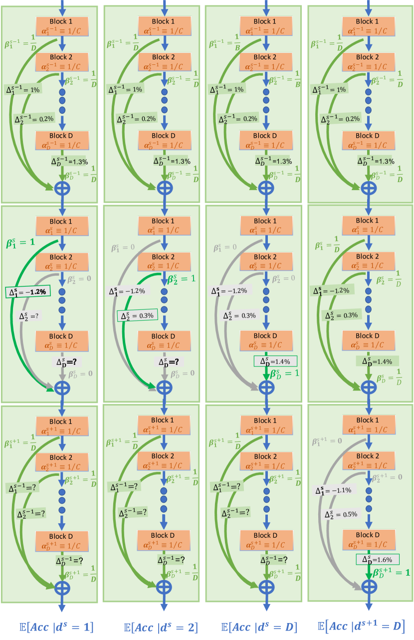
Figure 11: Extension of Figure 4: Estimating the expected accuracy gap caused by macroscopic design choices of the depth of the stages.

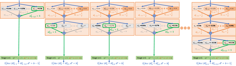
Figure 12: Extension of Figure 5: Estimating the expected accuracy gap caused by microscopic design choices on the operation applied at every block one at a time.

References

• [1] Bender, G., Kindermans, P.J., Zoph, B., Vasudevan, V., Le, Q.: Understanding and simplifying one-shot architecture search. In: International Conference on Machine Learning. pp. 550–559. PMLR (2018)
• [2] Bottou, L.: Online algorithms and stochastic approxima-p tions. Online learning and neural networks (1998)
• [3] Brock, A., Lim, T., Ritchie, J.M., Weston, N.: Smash: one-shot model architecture search through hypernetworks. arXiv preprint arXiv:1708.05344 (2017)
• [4] Cai, H., Gan, C., Wang, T., Zhang, Z., Han, S.: Once-for-all: Train one network and specialize it for efficient deployment. arXiv preprint arXiv:1908.09791 (2019)
• [5] Cai, H., Zhu, L., Han, S.: Proxylessnas: Direct neural architecture search on target task and hardware. arXiv preprint arXiv:1812.00332 (2018)
• [6] Chen, X., Xie, L., Wu, J., Tian, Q.: Progressive differentiable architecture search: Bridging the depth gap between search and evaluation. In: Proceedings of the IEEE International Conference on Computer Vision. pp. 1294–1303 (2019)
• [7] Chu, X., Zhang, B., Xu, R., Li, J.: Fairnas: Rethinking evaluation fairness of weight sharing neural architecture search. arXiv preprint arXiv:1907.01845 (2019)
• [8] Cubuk, E.D., Zoph, B., Mane, D., Vasudevan, V., Le, Q.V.: Autoaugment: Learning augmentation policies from data. arXiv preprint arXiv:1805.09501 (2018)
• [9] Deng, J., Dong, W., Socher, R., Li, L.J., Li, K., Fei-Fei, L.: ImageNet: A Large-Scale Hierarchical Image Database. In: CVPR09 (2009)
• [10] Frank, M., Wolfe, P., et al.: An algorithm for quadratic programming. Naval research logistics quarterly 3(1-2), 95–110 (1956)
• [11] Gallo, G., Ülkücü, A.: Bilinear programming: an exact algorithm. Mathematical Programming 12(1), 173–194 (1977)
• [12] Guo, Z., Zhang, X., Mu, H., Heng, W., Liu, Z., Wei, Y., Sun, J.: Single path one-shot neural architecture search with uniform sampling. In: European Conference on Computer Vision. pp. 544–560. Springer (2020)
• [13] Hazan, E., Luo, H.: Variance-reduced and projection-free stochastic optimization. In: International Conference on Machine Learning. pp. 1263–1271. PMLR (2016)
• [14] He, K., Zhang, X., Ren, S., Sun, J.: Deep residual learning for image recognition. 2016 IEEE Conference on Computer Vision and Pattern Recognition (CVPR) pp. 770–778 (2015)
• [15] Hinton, G., Vinyals, O., Dean, J.: Distilling the knowledge in a neural network. In: NIPS Deep Learning and Representation Learning Workshop (2015), http://arxiv.org/abs/1503.02531
• [16] Howard, A., Pang, R., Adam, H., Le, Q.V., Sandler, M., Chen, B., Wang, W., Chen, L., Tan, M., Chu, G., Vasudevan, V., Zhu, Y.: Searching for mobilenetv3. In: 2019 IEEE/CVF International Conference on Computer Vision, ICCV 2019, Seoul, Korea (South), October 27 - November 2, 2019. pp. 1314–1324. IEEE (2019). https://doi.org/10.1109/ICCV.2019.00140, https://doi.org/10.1109/ICCV.2019.00140
• [17] Hu, J., Shen, L., Sun, G.: Squeeze-and-excitation networks. In: Proceedings of the IEEE conference on computer vision and pattern recognition. pp. 7132–7141 (2018)
• [18] Hu, Y., Wu, X., He, R.: Tf-nas: Rethinking three search freedoms of latency-constrained differentiable neural architecture search. arXiv preprint arXiv:2008.05314 (2020)
• [19] Huang, Y., Cheng, Y., Bapna, A., Firat, O., Chen, D., Chen, M., Lee, H., Ngiam, J., Le, Q.V., Wu, Y., et al.: Gpipe: Efficient training of giant neural networks using pipeline parallelism. In: Advances in neural information processing systems. pp. 103–112 (2019)
• [20] Ibm ilog cplex miqcp optimizer. https://www.ibm.com/docs/en/icos/12.7.1.0?topic=smippqt-miqcp-mixed-integer-programs-quadratic-terms-in-constraints
• [21] Intel(R): Intel(r) math kernel library for deep neural networks (intel(r) mkl-dnn) (2019), https://github.com/rsdubtso/mkl-dnn
• [22] Kellerer, H., Pferschy, U., Pisinger, D.: The Multiple-Choice Knapsack Problem, pp. 317–347. Springer Berlin Heidelberg, Berlin, Heidelberg (2004). https://doi.org/10.1007/978-3-540-24777-7_11, https://doi.org/10.1007/978-3-540-24777-7_11
• [23] Kelley, H.J.: Gradient theory of optimal flight paths. Ars Journal 30(10), 947–954 (1960)
• [24] Lacoste-Julien, S., Jaggi, M., Schmidt, M., Pletscher, P.: Block-coordinate frank-wolfe optimization for structural svms. In: International Conference on Machine Learning. pp. 53–61. PMLR (2013)
• [25] Langford, E., Schwertman, N., Owens, M.: Is the property of being positively correlated transitive? The American Statistician 55(4), 322–325 (2001)
• [26] Liang, H., Zhang, S., Sun, J., He, X., Huang, W., Zhuang, K., Li, Z.: Darts+: Improved differentiable architecture search with early stopping. arXiv preprint arXiv:1909.06035 (2019)
• [27] Liu, H., Simonyan, K., Yang, Y.: Darts: Differentiable architecture search. arXiv preprint arXiv:1806.09055 (2018)
• [28] Lu, Z., Deb, K., Goodman, E., Banzhaf, W., Boddeti, V.N.: NSGANetV2: Evolutionary multi-objective surrogate-assisted neural architecture search. In: European Conference on Computer Vision (ECCV) (2020)
• [29] Nayman, N., Aflalo, Y., Noy, A., Zelnik-Manor, L.: Hardcore-nas: Hard constrained differentiable neural architecture search. arXiv preprint arXiv:2102.11646 (2021)
• [30] Nayman, N., Noy, A., Ridnik, T., Friedman, I., Jin, R., Zelnik, L.: Xnas: Neural architecture search with expert advice. In: Advances in Neural Information Processing Systems. pp. 1977–1987 (2019)
• [31] Noy, A., Nayman, N., Ridnik, T., Zamir, N., Doveh, S., Friedman, I., Giryes, R., Zelnik, L.: Asap: Architecture search, anneal and prune. In: International Conference on Artificial Intelligence and Statistics. pp. 493–503. PMLR (2020)
• [32] Padberg, M., Rinaldi, G.: A branch-and-cut algorithm for the resolution of large-scale symmetric traveling salesman problems. SIAM review 33(1), 60–100 (1991)
• [33] Paszke, A., Gross, S., Massa, F., Lerer, A., Bradbury, J., Chanan, G., Killeen, T., Lin, Z., Gimelshein, N., Antiga, L., Desmaison, A., Kopf, A., Yang, E., DeVito, Z., Raison, M., Tejani, A., Chilamkurthy, S., Steiner, B., Fang, L., Bai, J., Chintala, S.: Pytorch: An imperative style, high-performance deep learning library. In: Wallach, H., Larochelle, H., Beygelzimer, A., d'Alché-Buc, F., Fox, E., Garnett, R. (eds.) Advances in Neural Information Processing Systems 32, pp. 8024–8035. Curran Associates, Inc. (2019)
• [34] Real, E., Aggarwal, A., Huang, Y., Le, Q.V.: Regularized evolution for image classifier architecture search. In: Proceedings of the aaai conference on artificial intelligence. vol. 33, pp. 4780–4789 (2019)
• [35] Ru, B., Wan, X., Dong, X., Osborne, M.: Interpretable neural architecture search via bayesian optimisation with weisfeiler-lehman kernels. In: International Conference on Learning Representations (2021), https://openreview.net/forum?id=j9Rv7qdXjd
• [36] Rumelhart, D.E., Hinton, G.E., Williams, R.J.: Learning internal representations by error propagation. Tech. rep., California Univ San Diego La Jolla Inst for Cognitive Science (1985)
• [37] Sandler, M., Howard, A., Zhu, M., Zhmoginov, A., Chen, L.C.: Mobilenetv2: Inverted residuals and linear bottlenecks. In: Proceedings of the IEEE conference on computer vision and pattern recognition. pp. 4510–4520 (2018)
• [38] Simonyan, K., Zisserman, A.: Very deep convolutional networks for large-scale image recognition. In: International Conference on Learning Representations (2015)
• [39] Stamoulis, D., Ding, R., Wang, D., Lymberopoulos, D., Priyantha, B., Liu, J., Marculescu, D.: Single-path nas: Designing hardware-efficient convnets in less than 4 hours. In: Joint European Conference on Machine Learning and Knowledge Discovery in Databases. pp. 481–497. Springer (2019)
• [40] Szegedy, C., Vanhoucke, V., Ioffe, S., Shlens, J., Wojna, Z.: Rethinking the inception architecture for computer vision. In: Proceedings of the IEEE conference on computer vision and pattern recognition. pp. 2818–2826 (2016)
• [41] Tan, M., Chen, B., Pang, R., Vasudevan, V., Sandler, M., Howard, A., Le, Q.V.: Mnasnet: Platform-aware neural architecture search for mobile. In: Proceedings of the IEEE Conference on Computer Vision and Pattern Recognition. pp. 2820–2828 (2019)
• [42] Tan, M., Le, Q.V.: Efficientnet: Rethinking model scaling for convolutional neural networks. In: Chaudhuri, K., Salakhutdinov, R. (eds.) Proceedings of the 36th International Conference on Machine Learning, ICML 2019, 9-15 June 2019, Long Beach, California, USA. Proceedings of Machine Learning Research, vol. 97, pp. 6105–6114. PMLR (2019), http://proceedings.mlr.press/v97/tan19a.html
• [43] Wang, R., Cheng, M., Chen, X., Tang, X., Hsieh, C.J.: Rethinking architecture selection in differentiable nas. arXiv preprint arXiv:2108.04392 (2021)
• [44] White, C., Zela, A., Ru, B., Liu, Y., Hutter, F.: How powerful are performance predictors in neural architecture search? arXiv preprint arXiv:2104.01177 (2021)
• [45] Wu, B., Dai, X., Zhang, P., Wang, Y., Sun, F., Wu, Y., Tian, Y., Vajda, P., Jia, Y., Keutzer, K.: Fbnet: Hardware-aware efficient convnet design via differentiable neural architecture search. In: IEEE Conference on Computer Vision and Pattern Recognition, CVPR 2019, Long Beach, CA, USA, June 16-20, 2019. pp. 10734–10742. Computer Vision Foundation / IEEE (2019). https://doi.org/10.1109/CVPR.2019.01099
• [46] Zoph, B., Le, Q.V.: Neural architecture search with reinforcement learning. arXiv preprint arXiv:1611.01578 (2016)