Deep Learning Approximation of Diffeomorphisms via Linear-Control Systems

Abstract.

In this paper we propose a Deep Learning architecture to approximate diffeomorphisms diffeotopic to the identity. We consider a control system of the form $\dot{x}=\sum_{i=1}^{l}F_{i}(x)u_{i}$, with linear dependence in the controls, and we use the corresponding flow to approximate the action of a diffeomorphism on a compact ensemble of points. Despite the simplicity of the control system, it has been recently shown that a Universal Approximation Property holds. The problem of minimizing the sum of the training error and of a regularizing term induces a gradient flow in the space of admissible controls. A possible training procedure for the discrete-time neural network consists in projecting the gradient flow onto a finite-dimensional subspace of the admissible controls. An alternative approach relies on an iterative method based on Pontryagin Maximum Principle for the numerical resolution of Optimal Control problems. Here the maximization of the Hamiltonian can be carried out with an extremely low computational effort, owing to the linear dependence of the system in the control variables. Finally, we use tools from $\Gamma$-convergence to provide an estimate of the expected generalization error.

Keywords

Deep Learning, Linear-Control System, $\Gamma$-convergence, Gradient Flow, Pontryagin Maximum Principle.

MSC2020 classification

Primary: 49M05, 49M25. Secondary: 68T07, 49J15.

1. Introduction

Residual Neural Networks (ResNets) were originally introduced in [18] in order to overcome some issues related to the training process of traditional Deep Learning architectures. Indeed, it had been observed that, as the number of the layers in non-residual architectures is increased, the learning of the parameters is affected by the vanishing of the gradients (see, e.g., [7]) and the accuracy of the network gets rapidly saturated (see [17]). ResNets can be represented as the composition of non-linear mappings

$$\Phi=\Phi_{N}\circ\ldots\circ\Phi_{1},$$

where $N$ represents the depth of the Neural Network and, for every $k=1\ldots N$, the building blocks $\Phi_{k}:\mathbb{R}^{n}\to\mathbb{R}^{n}$ are of the form

$$\Phi_{k}(x)=x+\sigma(W_{k}x+b_{k}),$$ (1.1)

where $\sigma:\mathbb{R}^{n}\to\mathbb{R}^{n}$ is a non-linear activation function that acts component-wise, and $W_{k}\in\mathbb{R}^{n\times n}$ and $b_{k}\in\mathbb{R}^{n}$ are the parameters to be learned. In contrast, we recall that in non-residual architectures $\bar{\Phi}=\bar{\Phi}_{N}\circ\ldots\circ\bar{\Phi}_{1}$, the building blocks have usually the form

$$\bar{\Phi}_{k}(x)=\sigma(W_{k}x+b_{k})$$

for $k=1,\ldots,N$. In some recent contributions [14, 19, 16], ResNets have been studied in the framework of Mathematical Control Theory. The bridge between ResNets and Control Theory was independently discovered in [14] and [16], where it was observed that each function $\Phi_{1},\ldots,\Phi_{N}$ defined as in (1.1) can be interpreted as an Explicit Euler discretization of the control system

$$\dot{x}=\sigma(Wx+b),$$ (1.2)

where $W$ and $b$ are the control variables. Since then, Control Theory has been fruitfully applied to the theoretical understanding of ResNets. In [24] a Universal Approximation result for the flow generated by (1.2) was established under suitable assumptions on the activation function $\sigma$. In [19] and [8] the problem of learning an unknown mapping was formulated as an Optimal Control problem, and the Pontryagin Maximum Principle was employed in order to learn the optimal parameters. In [10] it was consider the mean-field limit of (1.2), and it was proposed a training algorithm based on the discretization of the necessary optimality conditions for an Optimal Control problem in the space of probability measures. The Maximum Principle for Optimal Control of probability measures was first introduced in [21], and recently it has been independently rediscovered in [9]. In this paper, rather than using tools from Control Theory to study properties of existing ResNets, we propose an architecture inspired by theoretical observations on control systems with linear dependence in the control variables. As a matter of fact, the building blocks of the ResNets that we shall construct depend linearly in the parameters, namely they have the form

$$\Phi_{k}(x)=x+G(x)u_{k},$$

where $G:\mathbb{R}^{n}\to\mathbb{R}^{n\times l}$ is a non-linear function of the input, and $u_{k}\in\mathbb{R}^{l}$ is the vector of the parameters at the $k$-th layer. The starting points of this paper are the controllability results proved in [4, 5], where the authors considered a control system of the form

$$\dot{x}=F(x)u=\sum_{i=1}^{l}F_{i}(x)u_{i},$$ (1.3)

where $F_{1},\ldots,F_{l}$ are smooth and bounded vector fields on $\mathbb{R}^{n}$, and $u\in\mathcal{U}:=L^{2}([0,1],\mathbb{R}^{l})$ is the control. We immediately observe that (1.3) has a simpler structure than (1.2), having linear dependence with respect to the control variables. Despite this apparent simplicity, the flows associated to (1.3) are capable of interesting approximating results. Given a control $u\in\mathcal{U}$, let $\Phi_{u}:\mathbb{R}^{n}\to\mathbb{R}^{n}$ be the flow obtained by evolving (1.3) on the time interval $[0,1]$ using the control $u$. In [5] it was formulated a condition for the controlled vector fields $F_{1},\ldots,F_{l}$ called Lie Algebra Strong Approximating Property. On one hand, this condition guarantees exact controllability on finite ensembles, i.e., for every $M\geq 1$, for every $\{x^{j}_{0}\}_{j=1,\ldots,M}\subset\mathbb{R}^{n}$ such that $j_{1}\neq j_{2}\implies x^{j_{1}}_{0}\neq x^{j_{2}}_{0}$, and for every injective mapping $\Psi:\mathbb{R}^{n}\to\mathbb{R}^{n}$, there exists a control $u\in\mathcal{U}$ such that $\Phi_{u}(x^{j}_{0})=\Psi(x^{j}_{0})$ for every $j=1,\ldots,M$. On the other hand, this property is also a sufficient condition for a $C^{0}$-approximate controllability result in the space of diffeomorphisms. More precisely, given a diffeomorphism $\Psi:\mathbb{R}^{n}\to\mathbb{R}^{n}$ diffeotopic to the identity, and given a compact set $K\subset\mathbb{R}^{n}$, for every $\varepsilon>0$ there exists a control $u_{\varepsilon}\in\mathcal{U}$ such that $\sup_{K}|\Phi_{u_{\varepsilon}}(x)-\Psi(x)|\leq\varepsilon$. The aim of this paper is to use this machinery to provide implementable algorithms for the approximation of diffeomorphisms diffeotopic to the identity. More precisely, we discretize the control system (1.3) on the evolution interval $[0,1]$ using the Explicit Euler scheme and the uniformly distributed time-nodes $\{0,\frac{1}{N},\ldots,\frac{N-1}{N},1\}$, and we obtain the ResNet represented by the composition $\Phi=\Phi_{N}\circ\ldots\circ\Phi_{1}$, where, for every $k=1,\ldots,N$, $\Phi_{k}$ is of the form

$$x_{k}=\Phi_{k}(x_{k-1})=x_{k-1}+h\sum_{i=1}^{l}F_{i}(x_{k-1})u_{i,k},\quad h=\frac{1}{N},$$ (1.4)

where $x_{0}\in\mathbb{R}^{n}$ represents an initial input of the network. In this construction, the points $(x_{k})_{k=0,\ldots,N}$ represent the approximations at the time-nodes $\{\frac{k}{N}\}_{k=0,\ldots,N}$ of the trajectory $x_{u}:[0,1]\to\mathbb{R}^{n}$ that solves (1.3) with Cauchy datum $x_{u}(0)=x_{0}$. We insist on the fact that in our discrete-time model we assume that the controls are piecewise constant on the time intervals $\left\{[\frac{k-1}{N},\frac{k}{N})\right\}_{k=1,\ldots,N}$. For this reason, when we derive a ResNet with $N$ hidden layers, we deal with $N$ building blocks (i.e., $\Phi_{1},\ldots,\Phi_{N}$) and with $N$ $l$-dimensional parameters $(u_{k})_{k=1,\ldots,N}=(u_{i,k})_{k=1,\ldots,N}^{i=1,\ldots,l}$. Moreover, when we evaluate the ResNet at a point $x_{0}\in\mathbb{R}^{n}$, we end up with $N+1$ input/output variables $(x_{k})_{k=0,\ldots,N}\subset\mathbb{R}^{n}$.

As anticipated before, we use the ResNet (1.4) for the task of a data-driven reconstruction of diffeomorphisms. The idea is that we may imagine to observe the action of an unknown diffeomorphism $\Psi:\mathbb{R}^{n}\to\mathbb{R}^{n}$ on a finite ensemble of points $\{x^{j}_{0}\}_{j=1,\ldots,M}$ with $M\geq 1$. Using these data, we try to approximate the mapping $\Psi$. Assuming that the controlled vector fields $F_{1},\ldots,F_{l}$ satisfy the Lie Algebra Strong Approximating Property, a first natural attempt consists in exploiting the exact controllability for finite ensembles. Indeed, this ensures that we can find a control $u^{M}\in\mathcal{U}$ that achieves a null training error, i.e., the corresponding flow $\Phi_{u^{M}}$ satisfies $\Phi_{u^{M}}(x^{j}_{0})=\Psi(x^{j}_{0})$ for every $j=1,\ldots,M$. Unfortunately, when the number of observation $M$ grows, this training strategy can not guarantee any theoretical upper bound for the generalization error. Indeed, as detailed in Section 4, in the case $\Psi$ is not itself a flow of the control system (1.3), if we pursue the null-training error strategy then the sequence of the controls $(u^{M})_{M\geq 1}$ will be unbounded in the $L^{2}$-norm. Since the Lipschitz constant of a flow generated by (1.3) is related to the $L^{2}$-norm of the corresponding control, it follows that we cannot bound from above the Lipschitz constants of the approximating diffeomorphisms $(\Phi_{u^{M}})_{M\geq 1}$. Therefore, even though for every $M\geq 1$ we achieve perfect matching $\Phi_{u^{M}}=\Psi$ on the training dataset $\{x_{0}^{j}\}_{j=1,\ldots,M}$, we have no control on the generalization error made outside the training points. This is an example of overfitting, a well-known phenomenon in the practice of Machine Learning.

In order to overcome this issue, when constructing the approximating diffeomorphism we need to find a balance between the training error and the $L^{2}$-norm of the control. For this reason we consider the non-linear functional $\mathcal{F}^{M}:\mathcal{U}\to\mathbb{R}$ defined on the space of admissible controls as follows:

$$\mathcal{F}^{M}(u):=\frac{1}{M}\sum_{j=1}^{M}a(\Phi_{u}(x^{j}_{0})-\Psi(x^{j}_{0}))+\frac{\beta}{2}||u||_{L^{2}}^{2},$$ (1.5)

where $a:\mathbb{R}^{n}\to\mathbb{R}$ is a non-negative function such that $a(0)=0$, and $\beta>0$ is a fixed parameter that tunes the squared $L^{2}$-norm regularization. A training strategy alternative to the one described above consists in looking for a minimizer $\tilde{u}^{M}$ of $\mathcal{F}^{M}$, and taking $\Phi_{\tilde{u}^{M}}$ as an approximation of $\Psi$. Under the assumption that the training dataset is sampled from a compactly-supported Borel probability measure $\mu$ on $\mathbb{R}^{n}$, we prove a $\Gamma$-convergence result. Namely, we show that, as the size $M$ of the training dataset tends to infinity, the problem of minimizing $\mathcal{F}^{M}$ converges to the problem of minimizing the functional $\mathcal{F}:\mathcal{U}\to\mathbb{R}$, defined as

$$\mathcal{F}(u):=\int_{\mathbb{R}^{n}}a(\Phi_{u}(x)-\Psi(x))\,d\mu(x)+\frac{\beta}{2}||u||_{L^{2}}^{2}.$$ (1.6)

Using this $\Gamma$-convergence result, we deduce the following upper bound for the expected testing error:

$$\mathbb{E}_{\mu}[a(\Phi_{\tilde{u}^{M}}(\cdot)-\Psi(\cdot))]\leq 2\kappa_{\beta}+C_{a,\Psi,\beta}W_{1}(\mu_{M},\mu),$$ (1.7)

where $\tilde{u}^{M}$ is a minimizer of $\mathcal{F}^{M}$, $\kappa_{\beta}$ and $C_{a,\Psi,\beta}$ are constants such that $\kappa_{\beta}\to 0$ and $C_{a,\Psi,\beta}\to\infty$ as $\beta\to 0$, and $W_{1}(\mu_{M},\mu)$ is the Wasserstein distance between $\mu$ and the empirical measure

$$\mu_{M}:=\frac{1}{M}\sum_{j=1}^{M}\delta_{x^{j}}.$$

Recalling that $W_{1}(\mu_{M},\mu)\to 0$ as $M\to\infty$, inequality (1.7) ensures that we can achieve arbitrarily small expected testing error by choosing $\beta$ small enough and having a large enough training dataset. Indeed, assuming that we can choose the size of the dataset, for every $\varepsilon>0$ we consider $\beta>0$ such that $\kappa_{\beta}\leq\frac{\varepsilon}{2}$, and then we take $M$ such that $C_{a,\Psi,\beta}W_{1}(\mu_{M},\mu)\leq\frac{\varepsilon}{2}$. We insist on the fact that the estimate in (1.7) holds a priori with respect to the choice of a testing dataset and the corresponding computation of the generalization error. We report that the minimization of the functional (1.6) plays a crucial role in [10].

On the base of the previous theoretical results, we propose two possible training algorithms to approximate the unknown diffeomorphism $\Psi$, having observed its action on an ensemble $\{x^{j}_{0}\}_{j=1,\ldots,M}$. The first one consists in introducing a finite-dimensional subspace $\mathcal{U}_{N}\subset\mathcal{U}$, and in projecting onto $\mathcal{U}_{N}$ the gradient flow induced by $\mathcal{F}^{M}$ in the space of admissible controls. Here we make use of the gradient flow formulation for optimal control problems derived in [23]. The second approach is based on the Pontryagin Maximum Principle, and it is similar to one followed in [19], [8], [10] for control system (1.2). We used the iterative method proposed in [22] for the the numerical resolution of Optimal Control problems. The main advantage of dealing with a linear-control system is that the maximization of the Hamiltonian (which is a key-step for the controls update) can be carried out with a low computational effort. In contrast, in [19] a non-linear optimization software was employed to manage this task, while in [10] the authors wrote the maximization as a root-finding problem and solved it with Brent’s method.
The paper is organized as follows. In Section 2 we establish the notations and we prove preliminary results regarding the flow generated by control system (1.3). In Section 3 we recall some results contained in [4] and [5] concerning exact and approximate controllability of ensembles. In Section 4 we explain why the “null training error strategy” is not suitable for the approximation purpose, and we outline the alternative strategy based on the resolution of an Optimal Control problem. In Section 5 we prove a $\Gamma$-convergence result that holds when the size $M$ of the training dataset tends to infinity. As a byproduct, we obtain the upper bound on the expected generalization error reported in (1.7). In Section 6 we describe the training algorithm based on the projection of the gradient flow induced by the cost $\mathcal{F}^{M}$. In Section 7 we propose the training procedure based on the Pontryagin Maximum Principle. In Section 8 we test numerically the algorithms by approximating a diffeomorphism in the plane.

2. Notations and Preliminary Results

In this paper we consider control systems of the form

$$\dot{x}=F(x)u=\sum_{i=1}^{l}F_{i}(x)u_{i},$$ (2.1)

where the controlled vector fields $(F_{i})_{i=1,\ldots,l}$ satisfy the following assumption.

Assumption 1.

The vector fields $F_{1},\ldots,F_{l}$ are smooth and bounded in $\mathbb{R}^{n}$, together with their derivatives of each order.

In particular, this implies that there exists $C_{1}>0$ such that

$$\sup_{i=1,\ldots,l}\,\,\sup_{x,y\in\mathbb{R}^{n}}\frac{|F_{i}(x)-F_{i}(y)|_{2}}{|x-y|_{2}}\leq C_{1}$$ (2.2)

The space of admissible controls is $\mathcal{U}:=L^{2}([0,1],\mathbb{R}^{l})$, endowed with the usual Hilbert space structure. Using Assumption 1, the classical Caratéodory Theorem guarantees that, for every $u\in\mathcal{U}$ and for every $x_{0}\in\mathbb{R}^{n}$, the Cauchy problem

$$\begin{cases}\dot{x}(s)=\sum_{i=1}^{l}F_{i}(x(s))u_{i}(s),\\ x(0)=x_{0},\end{cases}$$ (2.3)

has a unique solution $x_{u,x_{0}}:[0,1]\to\mathbb{R}^{n}$. Hence, for every $u\in\mathcal{U}$, we can define the flow $\Phi_{u}:\mathbb{R}^{n}\to\mathbb{R}^{n}$ as follows:

$$\Phi_{u}:x_{0}\mapsto x_{u,x_{0}}(1),$$ (2.4)

where $x_{u,x_{0}}$ solves (2.3). We recall that $\Phi_{u}$ is a diffeomorphism, since it is smooth and invertible.

In the paper we will make extensive use of the weak topology of $\mathcal{U}$. We recall that a sequence $(u_{\ell})_{\ell\geq 1}\subset\mathcal{U}$ is weakly convergent to an element $u\in\mathcal{U}$ if, for every $v\in\mathcal{U}$, we have that

$$\lim_{\ell\to\infty}\int_{0}^{1}v(s)u_{\ell}(s)\,ds=\int_{0}^{1}v(s)u(s)\,ds,$$

and we write $u_{\ell}\rightharpoonup_{L^{2}}u$. In the following result we consider a sequence of solutions of (2.3), corresponding to a weakly convergent sequence of controls.

Lemma 2.1.

Let $(u_{\ell})_{\ell\geq 1}\subset\mathcal{U}$ be a weakly convergent sequence, such that $u_{\ell}\rightharpoonup_{L^{2}}u$ as $\ell\to\infty$. For every $x_{0}\in\mathbb{R}^{n}$ and for every $\ell\geq 1$, let $x_{u_{\ell},x_{0}}:[0,1]\to\mathbb{R}^{n}$ be the solution of Cauchy problem (2.3) corresponding to the control $u_{\ell}$. Then

$$\lim_{\ell\to\infty}||x_{u_{\ell},x_{0}}-x_{u,x_{0}}||_{C^{0}}=0,$$

where $x_{u,x_{0}}:[0,1]\to\mathbb{R}^{n}$ is the solution of Cauchy problem (2.3) corresponding to the control $u$.

Proof.

Since the sequence $(u_{\ell})_{\ell\geq 1}$ is weakly convergent, it is bounded in $\mathcal{U}$. This fact and Assumption 1 imply that there exists a compact set $K\subset\mathbb{R}^{n}$ such that $x_{u_{\ell},x_{0}}(s)\in K$ for every $\ell\geq 1$ and for every $s\in[0,1]$. Moreover, being $(F_{i})_{i=1,\ldots,l}$ bounded, we deduce that

$$||\dot{x}_{u_{\ell},x_{0}}||_{L^{2}}\leq C||u_{l}||_{L^{2}}$$

for some constant $C>0$. Then it follows that the sequence is bounded in $W^{1,2}([0,1],\mathbb{R}^{n})$, and, as a matter of fact, that it is pre-compact with respect to the weak topology of $W^{1,2}$. Therefore, there exists a subsequence $(x_{u_{\ell_{k}},x_{0}})_{k\geq 1}$ and $x_{\infty}\in W^{1,2}$ such that $x_{u_{\ell_{k}},x_{0}}\rightharpoonup_{W^{1,2}}x_{\infty}$ as $k\to\infty$. Using the compact inclusion $W^{1,2}([0,1],\mathbb{R}^{n})\hookrightarrow C^{0}([0,1],\mathbb{R}^{n})$, we deduce that $x_{u_{\ell_{k}},x_{0}}\to_{C^{0}}x_{\infty}$. In particular, we obtain that $x_{\infty}(0)=x_{0}$. On the other hand, we have that $F(x_{u_{\ell_{k}},x_{0}})u_{\ell_{k}}\rightharpoonup_{L^{2}}F(x_{\infty})u$, since $F(x_{u_{\ell_{k}},x_{0}})\to_{C^{0}}F(x_{\infty})$. Recalling that $\dot{x}_{u_{\ell_{k}}}=F(x_{u_{\ell_{k}},x_{0}})u_{\ell_{k}}$ and that $x_{u_{\ell_{k}}}\rightharpoonup_{W^{1,2}}\dot{x}_{\infty}$ implies $\dot{x}_{u_{\ell_{k}}}\rightharpoonup_{L^{2}}\dot{x}_{\infty}$, we obtain that

$$\begin{cases}\dot{x}_{\infty}=F(x_{\infty})u,\\ x_{\infty}(0)=x_{0},\end{cases}$$

i.e., $x_{\infty}\equiv x_{u,x_{0}}$. Since the reasoning above is valid for every possible $W^{1,2}$-weak limiting point of $(x_{u_{\ell},x_{0}})_{\ell\geq 1}$, we deduce that the whole sequence is $W^{1,2}$-weakly convergent to $x_{u,x_{0}}$. Using again the compact inclusion $W^{1,2}([0,1],\mathbb{R}^{n})\hookrightarrow C^{0}([0,1],\mathbb{R}^{n})$, we deduce the thesis. ∎

We now prove an estimate of the Lipschitz constant of the flow $\Phi_{u}:\mathbb{R}^{n}\to\mathbb{R}^{n}$ for $u\in\mathcal{U}$.

Lemma 2.2.

For every admissible control $u\in\mathcal{U}$, let $\Phi_{u}:\mathbb{R}^{n}\to\mathbb{R}^{n}$ be corresponding flow defined in (2.4). Then $\Phi_{u}$ is Lipschitz-continuous with constant

$$L_{\Phi_{u}}\leq e^{C||u||_{L^{2}}},$$ (2.5)

where $C>0$ depends only on the controlled fields $(F_{i})_{i=1,\ldots,l}$ and on the dimension of the ambient space.

Proof.

For every $x_{0},w\in\mathbb{R}^{n}$ we have that $D_{x_{0}}\Phi_{u}(w)=v(1)$, where $v:[0,1]\to\mathbb{R}^{n}$ solves the linearized system

$$\begin{cases}\dot{v}(s)=\left(\sum_{i=1}^{l}u_{i}(s)D_{x}F_{i}(x_{u,x_{0}}(s))\right)v(s),\\ v(0)=w,\end{cases}$$

where $x_{u,x_{0}}:[0,1]\to\mathbb{R}^{n}$ is the controlled trajectory that solves (2.3), and for every $i=1,\ldots,l$ the expression $D_{x}F_{i}=(D_{x_{1}}F_{i},\ldots,D_{x_{n}}F_{i})$ denotes the Jacobian of the field $F_{i}$. Therefore, using (2.2), we deduce that

$$\frac{d}{ds}|v(s)|^{2}_{2}\leq 2C_{1}\left(\sum_{i=1}^{l}|u_{i}(s)|\right)|v(s)|^{2}_{2}.$$

Recalling that $\sum_{i=1}^{l}|u_{i}(s)|\leq\sqrt{n}|u(s)|_{2}$ and that

$$\int_{0}^{1}|u(s)|_{2}\,ds\leq\left(\int_{0}^{1}|u(s)|_{2}^{2}\,ds\right)^{\frac{1}{2}}=||u||_{L^{2}},$$

we deduce that

$$|v(1)|_{2}^{2}\leq e^{2C||u||_{L^{2}}}|v(0)|_{2}^{2},$$

where $C>0$ is a constant that depends only on $C_{1}$ and on the dimension $n$ of the ambient space. Finally this shows that

$$\frac{|D_{x_{0}}\Phi_{u}(w)|_{2}}{|w|_{2}}\leq e^{C||u||_{L^{2}}},$$

proving the thesis. ∎

The next result regards the convergence of the flows $(\Phi_{u_{\ell}})_{\ell\geq 1}$ corresponding to a weakly convergent sequence $(u_{\ell})_{\ell\geq 1}\subset\mathcal{U}$.

Proposition 2.3.

Given a sequence $(u_{\ell})_{\ell\geq 1}\subset\mathcal{U}$ such that $u_{\ell}\rightharpoonup_{L^{2}}u$ as $\ell\to\infty$ with respect to the weak topology of $\mathcal{U}$, then the flows $(\Phi_{u_{\ell}})_{\ell\geq 1}$ converge to $\Phi_{u}$ uniformly on compact sets.

Proof.

Let $K\subset\mathbb{R}^{n}$ be a compact set. For every $\ell\geq 1$ let us define $\Phi_{u_{\ell},K}:=\Phi_{u_{\ell}}|_{K}$, and $\Phi_{u,K}:=\Phi_{u}|_{K}$. Being weakly convergent, the sequence $(u_{\ell})_{\ell\geq 1}$ is bounded in $\mathcal{U}$. This fact and Assumption 1 imply that there exists a compact set $K^{\prime}\supset K$ such that any solution of (2.3) with initial datum in $K$ is entirely contained in $K^{\prime}$. In particular, we deduce that $\Phi_{u_{\ell}}(K)\subset K^{\prime}$ for every $\ell\geq 1$, i.e., the sequence $(\Phi_{u_{\ell},K})_{\ell\geq 1}$ is equi-bounded. Moreover, using the boundedness of $(u_{\ell})_{\ell\geq 1}\subset\mathcal{U}$ and Lemma 2.2, we obtain that $(\Phi_{u_{\ell},K})_{\ell\geq 1}$ is an equi-continuous family of diffeomorphisms. By Ascoli-Arzelà Theorem, it follows that $(\Phi_{u_{\ell},K})_{\ell\geq 1}$ is pre-compact with respect to the $C^{0}$ topology. On the other hand, Lemma 2.1 implies that for every $x\in K$ $\Phi_{u_{\ell},K}(x)\to\Phi_{u,K}(x)$ as $\ell\to\infty$. This guarantees that the set of limiting points with respect to the $C^{0}$ topology of the sequence $(\Phi_{u_{\ell},K})_{\ell\geq 1}$ is reduced to the single element $\Phi_{u,K}$. ∎

3. Ensemble Controllability

In this section we recall the most important results regarding the issue of ensemble controllability. For the proofs and the statements in full generality we refer the reader to [4] and [5]. We begin with the definition of ensemble in $\mathbb{R}^{n}$. In this section we will further assume that $n>1$, which is the most interesting case.

Definition 1.

Given a compact set $\Theta\subset\mathbb{R}^{n}$, an ensemble of points in $\mathbb{R}^{n}$ is an injective and continuous map $\gamma:\Theta\to\mathbb{R}^{n}$. We denote by $\mathcal{E}_{\Theta}(\mathbb{R}^{n})$ the space of ensembles.

Remark 3.1.

If $|\Theta|=M<\infty$, then an ensemble can be simply thought as an injective map from $\{1,\ldots,M\}$ to $\mathbb{R}^{n}$, or, equivalently, as an element of $(\mathbb{R}^{n})^{M}\setminus\Delta^{(M)}$, where

$$\Delta^{(M)}:=\{(x^{1},\ldots,x^{M})\in(\mathbb{R}^{n})^{M}:\exists j_{1}\neq j_{2}\mbox{ s.t. }x^{j_{1}}=x^{j_{2}}\}.$$

We define $(\mathbb{R}^{n})^{(M)}:=(\mathbb{R}^{n})^{M}\setminus\Delta^{(M)}$. Given a vector field $F:\mathbb{R}^{n}\to\mathbb{R}^{n}$, we define its $M$-fold vector field $F^{(M)}:(\mathbb{R}^{n})^{(M)}\to(\mathbb{R}^{n})^{(M)}$ as $F^{(M)}(x^{1},\ldots,x^{M})=(F(x^{1}),\ldots,F(x^{M}))$, for every $(x^{1},\ldots,x^{M})\in(\mathbb{R}^{n})^{(M)}$. Finally, we introduce the notation $\mathcal{E}_{M}(\mathbb{R}^{n})$ to denote the space of ensembles of $\mathbb{R}^{n}$ with $M$ elements.

We give the notion of reachable ensemble.

Definition 2.

The ensemble $\gamma(\cdot)\in\mathcal{E}_{\Theta}(\mathbb{R}^{n})$ is reachable from the ensemble $\alpha(\cdot)\in\mathcal{E}_{\Theta}(\mathbb{R}^{n})$ if there exists an admissible control $u\in\mathcal{U}$ such that its corresponding flow $\Phi_{u}$ defined in (2.4) satisfies:

$$\Phi_{u}(\alpha(\cdot))=\gamma(\cdot).$$

We can equivalently say that $\alpha(\cdot)$ can be steered to $\gamma(\cdot)$.

Definition 3.

Control system (2.1) is exactly controllable from $\alpha(\cdot)\in\mathcal{E}_{\Theta}(\mathbb{R}^{n})$ if every $\gamma(\cdot)\in\mathcal{E}_{\Theta}(\mathbb{R}^{n})$ is reachable from $\alpha(\cdot)$. The system is globally exactly controllable if it is exactly controllable from every $\alpha(\cdot)\in\mathcal{E}_{\Theta}(\mathbb{R}^{n})$.

We recall the definition of Lie algebra generated by a system of vector fields. Given the vector fields $F_{1},\ldots,F_{l}$, the linear space $\mathrm{Lie}(F_{1},\ldots,F_{l})$ is defined as

$$\mathrm{Lie}(F_{1},\ldots,F_{l}):=\mathrm{span}\{[F_{i_{s}},[\ldots,[F_{i_{2}},F_{i_{1}}]\ldots]]:s\geq 1,i_{1},\ldots,i_{s}\in\{1,\ldots,l\}\},$$ (3.1)

where $[F,F^{\prime}]$ denotes the Lie bracket between $F,F^{\prime}$, smooth vector fields of $\mathbb{R}^{n}$. In the case of finite ensembles, i.e., when $|\Theta|=M<\infty$, we can provide sufficient condition for controllability. The proof reduces to the classical Chow-Rashevsky theorem (see ,e.g, the textbook [1]).

Theorem 3.2.

Let $F_{1},\ldots,F_{l}$ be a system of vector fields on $\mathbb{R}^{n}$. Given $M\geq 1$, if for every $x^{(M)}=(x^{1},\ldots,x^{M})\in(\mathbb{R}^{n})^{(M)}$ the system of M-fold vector fields $F^{(M)}_{1},\ldots,F^{(M)}_{l}$ is bracket generating at $x^{(M)}$, i.e.,

$$\mathrm{Lie}(F^{(M)}_{1},\ldots,F^{(M)}_{l})|_{x^{(M)}}=(\mathbb{R}^{n})^{M},$$ (3.2)

then the control system (2.1) is globally exactly controllable on $\mathcal{E}_{M}(\mathbb{R}^{n})$.

For a finite ensemble, the global exact controllability holds for a generic system of vector fields.

Proposition 3.3.

For every $l\geq 2$, $M\geq 1$ and $m$ sufficiently large, then the $l$-tuples of vector fields $(F_{1},\ldots,F_{l})\in(\mathrm{Vect}(\mathbb{R}^{n}))^{l}$ such that system (2.1) is globally exactly controllable on $\mathcal{E}_{M}(\mathbb{R}^{n})$ is residual with respect to the Whitney $C^{m}$-topology.

We recall that a set is said residual if it is the complement of a countable union of nowhere dense sets. Proposition 3.3 means that, given any $l$-tuple $(F_{1},\ldots,F_{l})$ of vector fields, the corresponding control system (2.1) can be made globally exactly controllable in $\mathcal{E}_{M}(\mathbb{R}^{n})$ by means of an arbitrary small perturbation of the fields $F_{1},\ldots,F_{l}$ in the $C^{m}$-topology.

When dealing with infinite ensembles, the notions of “exact reachable” and “exact controllable” are too strong. However, they can be replaced by their respective $C^{0}$-approximate versions.

Definition 4.

The ensemble $\gamma(\cdot)\in\mathcal{E}_{\Theta}(\mathbb{R}^{n})$ is $C^{0}$-approximately reachable from the ensemble $\alpha(\cdot)\in\mathcal{E}_{\Theta}(\mathbb{R}^{n})$ if for every $\varepsilon>0$ there exists an admissible control $u\in\mathcal{U}$ such that its corresponding flow $\Phi_{u}$ defined in (2.4) satisfies:

$$\sup_{\Theta}|\Phi_{u}(\alpha(\cdot))-\gamma(\cdot)|_{2}<\varepsilon.$$ (3.3)

We can equivalently say that $\alpha(\cdot)$ can be $C^{0}$-approximately steered to $\gamma(\cdot)$.

Definition 5.

Control system (2.1) is $C^{0}$-approximately controllable from $\alpha(\cdot)\in\mathcal{E}_{\Theta}(\mathbb{R}^{n})$ if every $\gamma(\cdot)\in\mathcal{E}_{\Theta}(\mathbb{R}^{n})$ is $C^{0}$-approximately reachable from $\alpha(\cdot)$. The system is globally $C^{0}$-approximately controllable if it is $C^{0}$-approximately controllable from every $\alpha(\cdot)\in\mathcal{E}_{\Theta}(\mathbb{R}^{n})$.

Remark 3.4.

Let us further assume that the compact set $\Theta\subset\mathbb{R}^{n}$ has positive Lebesgue measure, and that it is equipped with a finite and positive measure $\mu$, absolutely continuous w.r.t. the Lebesgue measure. Then, the distance between the target ensemble $\gamma(\cdot)$ and the approximating ensemble $\Phi_{u}(\alpha(\cdot))$ can be quantified using the $L_{\mu}^{p}$-norm:

$$||\Phi_{u}(\alpha(\cdot))-\gamma(\cdot)||_{L_{\mu}^{p}}=\left(\int_{\Theta}|\Phi_{u}(\alpha(\theta))-\gamma(\theta)|_{2}^{p}\,d\mu(\theta)\right)^{\frac{1}{p}},$$

and we can equivalently formulate the notion of $L_{\mu}^{p}$-approximate controllability. In general, given a non-negative continuous function $a:\mathbb{R}^{n}\to\mathbb{R}$ such that $a(0)=0$, we can express the approximation error as

$$\int_{\Theta}a(\Phi_{u}(\alpha(\theta))-\gamma(\theta))\,d\mu(\theta).$$ (3.4)

In Section 5 we will consider an integral penalization term of this form. It is important to observe that, if $\gamma(\cdot)$ is $C^{0}$-approximately reachable from $\alpha(\cdot)$, then (3.4) can be made arbitrarily small.

Before stating the next result we introduce some notations. Given a vector field $X:\mathbb{R}^{n}\to\mathbb{R}^{n}$ and a compact set $K\subset\mathbb{R}^{n}$, we define

$$||X||_{1,K}:=\sup_{x\in K}\left(|X(x)|_{2}+\sum_{i=1}^{n}|D_{x_{i}}X(x)|_{2}\right).$$

Then we set

$$\mathrm{Lie}^{\delta}_{1,K}(F_{1},\ldots,F_{l}):=\{X\in\mathrm{Lie}(F_{1},\ldots,F_{l}):||X||_{1,K}\leq\delta\}.$$

We now formulate the assumption required for the approximability result.

Assumption 2.

The system of vector fields $F_{1},\ldots,F_{l}$ satisfies the Lie algebra strong approximating property, i.e., there exists $m\geq 1$ such that, for every $C^{m}$-regular vector field $Y:\mathbb{R}^{n}\to\mathbb{R}^{n}$ and for each compact set $K\subset\mathbb{R}^{n}$ there exists $\delta>0$ such that

$$\inf\left\{\sup_{x\in K}|X(x)-Y(x)|_{2}\,\,\Big{|}X\in\mathrm{Lie}_{1,K}^{\delta}(F_{1},\ldots,F_{l})\right\}=0.$$ (3.5)

The next result establishes a Universal Approximating Property for flows.

Theorem 3.5.

Let $\Psi:\mathbb{R}^{n}\to\mathbb{R}^{n}$ be a diffeomorphism diffeotopic to the identity. Let $F_{1},\ldots,F_{l}$ be a system of vector fields satisfying Assumptions 1 and 2. Then for each compact set $K\subset\mathbb{R}^{n}$ and each $\varepsilon>0$ there exists an admissible control $u\in\mathcal{U}$ such that

$$\sup_{x\in K}|\Psi(x)-\Phi_{u}(x)|_{2}\leq\varepsilon,$$ (3.6)

where $\Phi_{u}$ is the flow corresponding to the control $u$ defined in (2.4).

We recall that $\Psi:\mathbb{R}^{n}\to\mathbb{R}^{n}$ is diffeotopic to the identity if and only if there exists a family of diffeomorphisms $(\Psi_{s})_{s\in[0,1]}$ smoothly depending on $s$ such that $\Psi_{0}=\mathrm{Id}$ and $\Psi_{1}=\Psi$. In this case, $\Psi$ can be seen as the flow generated by the non-autonomous vector field $(s,x)\mapsto Y_{s}(x)$, where

$$Y_{s}(x):=\left.\frac{d}{d\varepsilon}\right|_{\varepsilon=0}\Psi_{s+\varepsilon}(x).$$

From Theorem 3.5 we can deduce a $C^{0}$-approximate reachability result for infinite ensembles.

Corollary 3.6.

Let $\alpha(\cdot),\beta(\cdot)\in\mathcal{E}_{\Theta}(\mathbb{R}^{n})$ be diffeotopic, i.e., there exists a diffeomorphism $\Psi:\mathbb{R}^{n}\to\mathbb{R}^{n}$ diffeotopic to the identity such that $\gamma=\Psi\circ\alpha$. Then $\gamma(\cdot)$ is $C^{0}$-approximate reachable from $\alpha(\cdot)$.

Remark 3.7.

If a system of vector fields satisfies Assumption 2, then, for every $M\geq 1$ and for every $x^{(M)}\in(\mathbb{R}^{n})^{(M)}$ Lie bracket generating condition (3.2) is automatically satisfied (see [5, Theorem 4.3]). This means that Assumption 2 guarantees global exact controllability in $\mathcal{E}_{M}(\mathbb{R}^{n})$, and $C^{0}$-approximate reachability for infinite diffeotopic ensembles.

We conclude this section with the exhibition of a system of vector fields in $\mathbb{R}^{n}$ meeting Assumptions 1 and 2.

Theorem 3.8.

For every $n>1$ and $\nu>0$, consider the vector fields in $\mathbb{R}^{n}$

$${\bar{F}_{i}}(x):=\frac{\partial}{\partial x_{i}},\quad{\bar{F}^{\prime}_{i}}(x):=e^{-\frac{1}{2\nu}|x|^{2}}\frac{\partial}{\partial x_{i}},\quad i=1,\ldots,n.$$ (3.7)

Then the system $\bar{F}_{1},\ldots,\bar{F}_{n},\bar{F}^{\prime}_{1},\ldots,\bar{F}^{\prime}_{n}$ satisfies Assumptions 1 and 2.

Remark 3.9.

If we consider the vector fields $\bar{F}_{1},\ldots,\bar{F}_{n},\bar{F}^{\prime}_{1},\ldots,\bar{F}^{\prime}_{n}$ defined in (3.7), then Theorem 3.5 and Theorem 3.8 guarantee that the flows generated by the corresponding linear-control system can approximate on compact sets diffeorphisms diffeotopic to the identity. From a theoretical viewpoint, this approximation result cannot be strengthened by enlarging the family of controlled vector fields, since the flows produced by any controlled dynamical system are themselves diffeotopic to the identity. On the other hand, in view of the discretization of the dynamics and the consequent construction of the ResNet, it could be useful to enrich the system of the controlled fields. As suggested by Assumption 2, the expressivity of the linear-control system is more directly related to the space $\mathrm{Lie}(F_{1},\ldots,F_{l})$, rather than to the family $F_{1},\ldots,F_{l}$ itself. However, as we are going to see, “reproducing” the flow of a field that belongs to $\mathrm{Lie}(F_{1},\ldots,F_{l})\setminus\mathrm{span}\{F_{1},\ldots,F_{l}\}$ can be expensive. Let us consider an evolution step-size $h\in(0,1/4)$ and let us choose two of the controlled vector fields, say $F_{1},F_{2}$, and let us assume that $[F_{1},F_{2}]\in\mathrm{Lie}(F_{1},\ldots,F_{l})\setminus\mathrm{span}\{F_{1},\ldots,F_{l}\}$. Let us denote by $e^{\pm hF_{i}}:\mathbb{R}^{n}\to\mathbb{R}^{n},i=1,2$ the flows obtained by evolving $\pm F_{i},i=1,2$ for an amount of time equal to $h$. Then, using for instance the computations in [1, Subsection 2.4.7], for every $x\in K$ compact we obtain that

$$\left(e^{-hF_{2}}\circ e^{-hF_{1}}\circ e^{hF_{2}}\circ e^{hF_{1}}\right)(x)=e^{h^{2}[F_{1},F_{2}]}(x)+o(h^{2})$$

as $h\to 0$. The previous computation shows that, in order to approximate the effect of evolving the vector field $[F_{1},F_{2}]$ for an amount of time equal to $h^{2}$, we need tho evolve the fields $\pm F_{i},i=1,2$ for a total amount $4h$. If $h$ represents the discretization step-size used to derive the ResNet (1.4) from the linear-control system (2.1) on the interval $[0,1]$, then we have that $h=\frac{1}{N}$, where $N$ is the number of layers of the ResNet. The argument above suggests that we need to use $4$ layers of the network to “replicate” the effect of evolving $[F_{1},F_{2}]$ for the amount of time $h^{2}=\frac{1}{N^{2}}$ (note that $h^{2}\ll h$ when $N\gg 1$). This observation provides an insight for the practical choice of the system of controlled fields. In first place, the system $F_{1},\ldots,F_{l}$ should meet Assumption 2. If the ResNet obtained from the discretization of the system does not seem to be expressive enough, it should be considered to enlarge the family of the controlled fields, for example by including some elements of $\mathrm{span}\{[F_{i_{1}},F_{i_{2}}]:i_{1},i_{2}\in\{1,\ldots,l\}\}$ (or, more generally, of $\mathrm{Lie}(F_{1},\ldots,F_{l})$). We insist on the fact that this procedure increases the width of the network, since the larger is the number of fields in the control system, the larger is the number of parameters per layer in the ResNet.

4. Approximation of Diffeomorphisms: Robust Strategy

In this section we introduce the central problem of the paper, i.e., the training of control system (2.1) in order to approximate an unknown diffeomorphism $\Psi:\mathbb{R}^{n}\to\mathbb{R}^{n}$ diffeotopic to the identity. A typical situation that may arise in applications is that we want to approximate $\Psi$ on a compact set $K\subset\mathbb{R}^{n}$, having observed the action of $\Psi$ on a finite number of training points $\{x^{1}_{0},\ldots,x^{M}_{0}\}\subset K$. Our aim is to formulate a strategy that is robust with respect to the size $M$ of the training dataset, and for which we can give upper bounds for the generalization error. In order to obtain higher and higher degree of approximation, we may thing to triangulate the compact set $K$ with an increasing number of nodes where we can evaluate the unknown map $\Psi$. Using the language introduced in Section 3, we have that, for every $M\geq 1$, we may understand a triangulation of $K$ with $M$ nodes as an ensemble $\alpha^{M}(\cdot)\in\mathcal{E}_{M}(\mathbb{R}^{n})$. After evaluating $\Psi$ in the nodes, we obtain the target ensemble $\gamma^{M}(\cdot)\in\mathcal{E}_{M}(\mathbb{R}^{n})$ as $\gamma^{M}(\cdot):=\Psi(\alpha^{M}(\cdot))$.

If the vector fields $F_{1},\ldots,F_{l}$ that define control system (2.1) meet Assumptions 1 and 2, then Theorem 3.2 and Remark 3.7 may suggest a first natural attempt to design an approximation strategy. Indeed, for every $M$, we can exactly steer the ensemble $\alpha^{M}(\cdot)$ to the ensemble $\gamma^{M}(\cdot)$ with an admissible control $u^{M}\in\mathcal{U}$. Hence, we can choose the flow $\Phi_{u^{M}}$ defined in (2.4) as an approximation of $\Psi$ on $K$, achieving a null training error. Assume that, for every $M\geq 1$, the corresponding triangulation is a $\epsilon^{M}$-approximation of the set $K$, i.e., for every $y\in K$ there exists $\bar{j}\in\{1,\ldots,M\}$ such that $|y-x^{\bar{j},M}_{0}|_{2}\leq\epsilon^{M}$, where $x^{\bar{j},M}_{0}:=\alpha^{M}(\bar{j})$. Then, for every $y\in K$, we can give the following estimate for the generalization error:

$$|\Psi(y)-\Phi_{u^{M}}(y)|_{2} \leq|\Psi(y)-\Psi(x^{\bar{j},M}_{0})|_{2}+|\Phi_{u^{M}}(x^{\bar{j},M}_{0})-\Phi_{u^{M}}(y)|_{2}$$

$$\leq L_{\Psi}\epsilon^{M}+L_{\Phi_{u^{M}}}\epsilon^{M},$$

where $L_{\Psi},L_{\Phi_{u^{M}}}$ are respectively the Lipschitz constants of $\Psi$ and $\Phi_{u^{M}}$. Assuming (as it is natural to do) that $\epsilon^{M}\to 0$ as $M\to\infty$, the strategy of achieving zero training error works if, for example, the Lipschitz constants of the approximating flows $(\Phi_{u^{M}})_{M\geq 1}$ keep bounded. This in turn would follow if the sequence of controls $(u^{M})_{M\geq 1}$ were bounded in $L^{2}$-norm. However, as we are going to see in the following proposition, in general this is not the case. Let us define

$$\mathrm{Flows}_{K}(F_{1},\ldots,F_{l}):=\{\Phi_{u}:u\in\mathcal{U}\},$$

the space of flows restricted to $K$ obtained via (2.4) with admissible controls, and let $\mathrm{Diff}_{K}^{0}(\mathbb{R}^{n})$ be the space of diffeomorphisms diffeotopic to the identity restricted to $K$. Theorem 3.5 guarantees that, for every $K\subset\mathbb{R}^{n}$,

$$\overline{\mathrm{Flows}_{K}(F_{1},\ldots,F_{l})}^{C^{0}}=\mathrm{Diff}_{K}^{0}(\mathbb{R}^{n}).$$

Proposition 4.1.

Given a diffeomorphism $\Psi\in\mathrm{Diff}_{K}^{0}(\mathbb{R}^{n})\setminus\mathrm{Flows}_{K}(F_{1},\ldots,F_{l})$ and an approximating sequence $(\Phi_{u_{\ell}})_{\ell\geq 1}\subset\mathrm{Flows}_{K}(F_{1},\ldots,F_{l})$ such that $\Phi_{u_{\ell}}\to_{C^{0}}\Psi$ on $K$, then the sequence of controls $(u_{\ell})_{\ell\geq 1}\subset\mathcal{U}$ is unbounded in the $L^{2}$-norm.

Proof.

By contradiction, let $(u_{\ell})_{\ell\geq 1}$ be a bounded sequence in $\mathcal{U}$. Then, we can extract a subsequence $(u_{\ell_{k}})_{k\geq 1}$ weakly convergent to $u\in\mathcal{U}$. In virtue of Proposition 2.3, we have that $\Phi_{u_{\ell_{k}}}\to_{C^{0}}\Phi_{u}$ on $K$. However, since $\Phi_{u_{\ell}}\to_{C^{0}}\Psi$ on $K$, we deduce that $\Psi=\Phi_{u}$ on $K$, but this contradicts the hypothesis $\Psi\in\mathrm{Diff}_{K}^{0}(\mathbb{R}^{n})\setminus\mathrm{Flows}_{K}(F_{1},\ldots,F_{l})$. ∎

The previous result sheds light on a weakness of the approximation strategy described above. Indeed, the main drawback is that we have no bounds on the norm of the controls $(u^{M})_{M\geq 1}$, and therefore, even though the triangulation of $K$ is fine, we cannot give an a priori estimate of the testing error. We point out that, in the different framework of simultaneous control of several systems, a similar situation was described in [3].

4.1. Approximation via Optimal Control

In order to avoid the issues described above, we propose a training strategy based on the solution of an Optimal Control problem with a regularization term penalizing the $L^{2}$-norm of the control. Namely, given a set of training points $\{x^{1}_{0},\ldots,x^{M}_{0}\}\subset K$, we consider the nonlinear functional $\mathcal{F}^{M}:\mathcal{U}\to\mathbb{R}$ defined as follows:

$$\mathcal{F}^{M}(u):=\frac{1}{M}\sum_{j=1}^{M}a(\Phi_{u}(x^{j}_{0})-\Psi(x^{j}_{0}))+\frac{\beta}{2}||u||^{2}_{L^{2}},$$ (4.1)

where $a:\mathbb{R}^{n}\to\mathbb{R}$ is a smooth loss function such that $a\geq 0$ and $a(0)=0$, and $\beta>0$ is a fixed parameter. The functional $\mathcal{F}^{M}$ is composed by two competing terms: the first aims at achieving a low mean training error, while the second aims at keeping bounded the $L^{2}$-norm of the control. In this framework, it is worth assuming that the compact set $K$ is equipped with a Borel probability measure $\mu$. In this way, we can give higher weight to the regions in $K$ where we need more accuracy in the approximation. As done before, for every $M\geq 1$ we understand the training dataset as an ensemble $\alpha^{M}(\cdot)\in\mathcal{E}_{M}(\mathbb{R}^{n})$. Moreover, we associate to it the discrete probability measure $\mu_{M}$ defined as

$$\mu_{M}:=\frac{1}{M}\sum_{j=1}^{M}\delta_{\alpha(j)},$$ (4.2)

and we can equivalently express the mean training error as

$$\frac{1}{M}\sum_{j=1}^{M}a(\Phi_{u}(x^{j}_{0})-\Psi(x^{j}_{0}))=\int_{\mathbb{R}^{n}}a(\Phi_{u}(x)-\Psi(x))\,d\mu_{M}(x).$$

From now on, when considering datasets growing in size, we make the following assumption on the sequence of probability measures $(\mu_{M})_{M\geq 1}$.

Assumption 3.

There exists a Borel probability measure $\mu$ supported in the compact set $K\subset\mathbb{R}^{n}$ such that the sequence $(\mu_{M})_{M\geq 1}$ is weakly convergent to $\mu$, i.e.,

$$\lim_{M\to\infty}\int_{\mathbb{R}^{n}}f(x)\,d\mu_{M}=\int_{\mathbb{R}^{n}}f(x)\,d\mu,$$ (4.3)

for every bounded continuous function $f:\mathbb{R}^{n}\to\mathbb{R}$. Moreover, we ask that $\mu_{M}$ is supported in $K$ for every $M\geq 1$.

Remark 4.2.

The request of Assumption 3 is rather natural. Indeed, if the elements of the ensembles $\alpha^{M}(\cdot)\in\mathcal{E}_{M}(\mathbb{R}^{n})$ are sampled using the probability distribution $\mu$ associated to the compact set $K$, it follows from the law of large numbers that (4.3) holds. On the other hand, since we ask that all the ensembles are contained in the compact set $K$, we have that the sequence of probability measures $(\mu_{M})_{M\geq 1}$ is tight. Therefore, in virtue of Prokhorov Theorem, $(\mu_{M})_{M\geq 1}$ is sequentially weakly pre-compact (for details see, e.g., [12]).

Remark 4.3.

When $K=\overline{\mathrm{int}(K)}$, if for every $M$ $\alpha^{M}(\cdot)$ is a $\epsilon^{M}$-approximation of $K$ such that $\epsilon^{M}\to 0$ as $M\to\infty$, then the corresponding sequence of probability measures $(\mu_{M})_{M\geq 1}$ is weakly convergent to $\mu=\mathcal{L}|_{K}$, where $\mathcal{L}$ denotes the Lebesgue measure in $\mathbb{R}^{n}$.

In the next result we prove that the functional $\mathcal{F}^{M}$ attains minimum for every $M\geq 1$. Moreover, we can give an upper bound for the $L^{2}$-norm of the minimizers of $\mathcal{F}^{M}$ that does not depend on $M$.

Proposition 4.4.

For every $M\geq 1$ the functional $\mathcal{F}^{M}:\mathcal{U}\to\mathbb{R}$ defined in (5.1) admits a minimizer. Moreover, if Assumption 3 is met, then there exists $C_{\beta}>0$ such that, for every $M\geq 1$, any minimizer $\tilde{u}^{M}$ of $\mathcal{F}^{M}$ satisfies the following inequality:

$$||\tilde{u}^{M}||_{L^{2}}\leq C_{\beta}.$$ (4.4)

Proof.

The existence of minimizers descends from the direct method of Calculus of Variations, since for every $M\geq 1$ the functional $\mathcal{F}^{M}$ is coercive and lower semi-continuous with respect to the weak topology of $\mathcal{U}$. Indeed, recalling that $a\geq 0$, we have that

$$\{u\in\mathcal{U}:\mathcal{F}^{M}(u)\leq c\}\subset\{u\in\mathcal{U}:\beta||u||_{L^{2}}^{2}\leq 2c\},$$

and this shows that $\mathcal{F}^{M}$ is coercive, for every $M\geq 1$. As regards the lower semi-continuity, let us consider a sequence $(u_{\ell})_{\ell\geq 1}\subset\mathcal{U}$ such that $u_{\ell}\rightharpoonup u$ as $\ell\to\infty$. Using Proposition 2.3 and the Dominated Convergence Theorem, for every $M\geq 1$ we have that

$$\lim_{\ell\to\infty}\int_{\mathbb{R}^{n}}a(\Phi_{u_{\ell}}(x)-\Psi(x))\,d\mu_{M}(x)=\int_{\mathbb{R}^{n}}a(\Phi_{u}(x)-\Psi(x))\,d\mu_{M}(x).$$

Finally, recalling that

$$||u||_{L^{2}}^{2}\leq\liminf_{\ell\to\infty}||u_{\ell}||_{L^{2}}^{2},$$

we deduce that for every $M\geq 1$ the functional $\mathcal{F}^{M}$ is lower semi-continuous.

We now prove the uniform estimate on the norm of minimizers. For every $M\geq 1$, let $\tilde{u}^{M}$ be a minimizer of $\mathcal{F}^{M}$. If we consider $v\equiv 0$, recalling that $\Phi_{v}=\mathrm{Id}$, we have that

$$\mathcal{F}^{M}(\tilde{u}^{M})\leq\mathcal{F}^{M}(v)=\int_{\mathbb{R}^{n}}a(x-\Psi(x))\,d\mu_{M}.$$

Using the fact that $(\mu_{M})_{M\geq 1}$ are uniformly compactly supported, we deduce that there exists $C>0$ such that

$$\sup_{M\geq 1}\int_{\mathbb{R}^{n}}a(x-\Psi(x))\,d\mu_{M}\leq C.$$

Therefore, recalling that $a\geq 0$, we have that

$$\frac{\beta}{2}||\tilde{u}^{M}||^{2}_{L^{2}}\leq C,$$

for every $M\geq 1$. This concludes the proof. ∎

The previous result suggests as a training strategy to look for a minimizer of the functional $\mathcal{F}^{M}$. In the next section we investigate the properties of the functionals $(\mathcal{F}^{M})_{M\geq 1}$ using the the tools of $\Gamma$-convergence.

5. Ensembles growing in size and $\Gamma$-convergence

In this section we study the limiting problem when the size of the training dataset tends to infinity. The main fact is that a $\Gamma$-convergence result holds. Roughly speaking, this means that increasing the size of the training dataset does not make the problem harder, at least from a theoretical viewpoint. For a thorough introduction to the subject, the reader is referred to [13].

For every $M\geq 1$, let $\alpha^{M}(\cdot)\in\mathcal{E}_{M}(\mathbb{R}^{n})$ be an ensemble of points in the compact set $K\subset\mathbb{R}^{n}$, and let us consider the discrete probability measure $\mu_{M}$ defined in (4.2). For every $M\geq 1$ we consider the functional $\mathcal{F}^{M}:\mathcal{U}\to\mathbb{R}$ defined as follows:

$$\mathcal{F}^{M}(u):=\int_{\mathbb{R}^{n}}a(\Phi_{u}(x)-\Psi(x))\,d\mu_{M}+\frac{\beta}{2}||u||^{2}_{L^{2}}.$$ (5.1)

The tools of $\Gamma$-convergence requires the domain where the functionals are defined to be equipped with a metrizable topology. Recalling that the weak topology of $L^{2}$ is metrizable only on bounded sets, we need to properly restrict the functionals. For every $\rho>0$, we set

$$\mathcal{U}_{\rho}:=\{u\in\mathcal{U}:||u||_{L^{2}}\leq\rho\}.$$

Using Proposition 4.4 we can choose $\rho=C_{\beta}$, so that

$$\arg\min_{\mathcal{U}}\mathcal{F}^{M}=\arg\min_{\mathcal{U}_{\rho}}\mathcal{F}^{M},$$

for every $M\geq 1$. With this choice we restrict the minimization problem to a bounded subset of $\mathcal{U}$, without losing any minimizer. We define $\mathcal{F}^{M}_{\rho}:=\mathcal{F}^{M}|_{\mathcal{U}_{\rho}}$. We recall the definition of $\Gamma$-convergence.

Definition 1.

The family of functionals $(\mathcal{F}^{M}_{\rho})_{M\geq 1}$ is said to $\Gamma$-converge to a functional $\mathcal{F}_{\rho}:\mathcal{U}_{\rho}\to\mathbb{R}\cup\{+\infty\}$ with respect to the weak topology of $\mathcal{U}$ as $M\to\infty$ if the following conditions hold:

• for every $(u^{M})_{M\in\mathbb{R}_{+}}\subset\mathcal{U}_{\rho}$ such that $u^{M}\rightharpoonup u$ as $M\to\infty$ we have

  $$\liminf_{M\to+\infty}\mathcal{F}^{M}_{\rho}(u^{M})\geq\mathcal{F}_{\rho}(u);$$ (5.2)

• for every $u\in\mathcal{U}$ there exists a sequence $(u^{M})_{M\in\mathbb{R}_{+}}\subset\mathcal{U}_{\rho}$ such that $u^{M}\rightharpoonup u$ as $M\to\infty$ and such that

  $$\limsup_{M\to+\infty}\mathcal{F}^{M}_{\rho}(u^{M})\leq\mathcal{F}_{\rho}(u).$$ (5.3)

If (5.2) and (5.3) are satisfied, then we write $\mathcal{F}^{M}_{\rho}\to_{\Gamma}\mathcal{F}_{\rho}$ as $M\to\infty$.

Let us define the functional $\mathcal{F}:\mathcal{U}\to\mathbb{R}$ as follows:

$$\mathcal{F}(u):=\int_{\mathbb{R}^{n}}a(\Phi_{u}(x)-\Psi(x))\,d\mu+\frac{\beta}{2}||u||_{L^{2}}^{2},$$ (5.4)

where the probability measure $\mu$ is the weak limit of the sequence $(\mu_{M})_{M\geq 1}$. Using the same argument as in the proof of Proposition 4.4, we can prove that $\mathcal{F}$ attains minimum and that

$$\arg\min_{\mathcal{U}}\mathcal{F}=\arg\min_{\mathcal{U}_{\rho}}\mathcal{F},$$

with $\rho=C_{\beta}$. As before, we define $\mathcal{F}_{\rho}:=\mathcal{F}|_{\mathcal{U}_{\rho}}$.

Theorem 5.1.

Given $\rho>0$, let us consider $\mathcal{F}^{M}_{\rho}:\mathcal{U}_{\rho}\to\mathbb{R}$ with $M\geq 1$. Let $\mathcal{F}_{\rho}:\mathcal{U}_{\rho}\to\mathbb{R}$ be the restriction to $\mathcal{U}_{\rho}$ of the functional defined in (5.4). If Assumption 3 holds, then the functionals $(\mathcal{F}^{M}_{\rho})_{M\geq 1}$ $\Gamma$-converge to $\mathcal{F}_{\rho}$ as $M\to\infty$ with respect to the weak topology of $\mathcal{U}$.

Proof.

Let us prove the $\limsup$-condition (5.3). Let us fix $u\in\mathcal{U}_{\rho}$ and, for every $M\geq 1$, let us define $u^{M}:=u$. Then, recalling that the measures $(\mu_{M})_{M\geq 1}$ are weakly convergent to $\mu$, we have that

$$\mathcal{F}_{\rho}(u)=\lim_{M\to\infty}\int_{\mathbb{R}^{n}}a(\Phi_{u}(x)-\Psi(x))\,d\mu_{M}+\frac{\beta}{2}||u||_{L^{2}}^{2}=\lim_{M\to\infty}\mathcal{F}^{M}_{\rho}(u).$$

This proves (5.3).

We now prove the $\liminf$-condition. Let $(u^{M})_{M\geq 1}\subset\mathcal{U}$ be weakly convergent to $u\in\mathcal{U}$. Using Proposition 2.3 we have that $\Phi_{u^{M}}|_{K}\to\Phi_{u}|_{K}$ with respect to the $C^{0}$ topology. Moreover, there exists a compact set $K^{\prime}\subset\mathbb{R}^{n}$ such that

$$(\Phi_{u}-\Psi)(K)\cup\bigcup_{M\geq 1}(\Phi_{u^{M}}-\Psi)(K)\subset K^{\prime}.$$

Using the fact that $a$ is uniformly continuous on $K^{\prime}$, we deduce that

$$\lim_{M\to\infty}\sup_{x\in K}|a(\Phi_{u^{M}}(x)-\Psi(x))-a(\Phi_{u}(x)-\Psi(x))|_{2}=0.$$ (5.5)

Using (5.5) and the weak convergence of $(\mu_{M})_{M\geq 1}$ to $\mu$, we deduce that

$$\lim_{M\to\infty}\int_{\mathbb{R}^{n}}a(\Phi_{u^{M}}(x)-\Psi(x))\,d\mu_{M}=\int_{\mathbb{R}^{n}}a(\Phi_{u}(x)-\Psi(x))\,d\mu.$$

Recalling that the $L^{2}$ norm is lower semi-continuous with respect to the weak convergence, we have that condition (5.2) is satisfied. ∎

Remark 5.2.

Using the equi-coercivity of the functionals $(\mathcal{F}^{M}_{\rho})_{M\geq 1}$ and [13, Corollary 7.20], we deduce that

$$\lim_{M\to\infty}\min_{\mathcal{U}_{\rho}}\mathcal{F}^{M}_{\rho}=\min_{\mathcal{U}_{\rho}}\mathcal{F}_{\rho},$$ (5.6)

and that any cluster point $\tilde{u}$ of a sequence of minimizers $(\tilde{u}^{M})_{M\geq 1}$ is a minimizer of $\mathcal{F}_{\rho}$. Let us assume that a sub-sequence $\tilde{u}^{M_{j}}\rightharpoonup\tilde{u}$ as $j\to\infty$. Using Proposition 2.3 and the Dominated Convergence Theorem we deduce that

$$\lim_{j\to\infty}\int_{K}a(\Phi_{\tilde{u}^{M_{j}}}(x)-\Psi(x))\,d\mu_{M}(x)=\int_{K}a(\Phi_{\tilde{u}}(x)-\Psi(x))\,d\mu(x),$$ (5.7)

where we stress that $\tilde{u}$ is a minimizer of $\mathcal{F}_{\rho}$. Combining (5.6) and (5.7) we obtain that

$$\lim_{j\to\infty}\frac{\beta}{2}||\tilde{u}^{M_{j}}||_{L^{2}}^{2}=\frac{\beta}{2}||\tilde{u}||_{L^{2}}^{2}.$$

Since $\tilde{u}^{M_{j}}\rightharpoonup\tilde{u}$ as $j\to\infty$, the previous equation implies that the subsequence $(\tilde{u}^{M_{j}})_{j\geq 1}$ converges to $\tilde{u}$ also with respect to the strong topology of $L^{2}$. This argument shows that any sequence of minimizers $(\tilde{u}^{M})_{M\geq 1}$ is pre-compact with respect to the strong topology of $L^{2}$.

We can establish an asymptotic upper bound for the mean training error. Let us define

$$\kappa_{\beta}:=\sup\left\{\int_{K}a(\Phi_{\tilde{u}}(x)-\Psi(x))\,d\mu(x)\bigg{|}\tilde{u}\in\arg\min_{\mathcal{U}}\mathcal{F}\right\}.$$ (5.8)

As suggested by the notation, the value of $\kappa_{\beta}$ highly depends on the positive parameter $\beta$ that tunes the $L^{2}$-regularization. Given a sequence of minimizers $(\tilde{u}^{M})_{M\geq 1}$ of the functionals $(\mathcal{F}^{M})_{M\geq 1}$, from (5.7) we deduce that

$$\limsup_{M\to\infty}\int_{K}a(\Phi_{\tilde{u}^{M}}(x)-\Psi(x))\,d\mu_{M}(x)\leq\kappa_{\beta}.$$ (5.9)

In the next result we show that under the hypotheses of Theorem 3.5 $\kappa_{\beta}$ can be made arbitrarily small with a proper choice of $\beta$.

Proposition 5.3.

Let $\kappa_{\beta}$ be defined as in (5.8). If the vector fields $F_{1},\ldots,F_{l}$ that define control system (2.1) satisfy Assumption 1 and 2, then

$$\lim_{\beta\to 0^{+}}\kappa_{\beta}=0.$$ (5.10)

Proof.

Let us fix $\varepsilon>0$. Since $a(0)=0$, there exists $\rho>0$ such that

$$\sup_{B_{\rho}(0)}a\leq\varepsilon.$$

Using Theorem 3.5, we deduce that there exists a control $\hat{u}\in\mathcal{U}$ such that

$$\sup_{x\in K}|\Phi_{\hat{u}}(x)-\Psi(x)|_{2}<\rho.$$ (5.11)

This implies that

$$\int_{K}a(\Phi_{\hat{u}}(x)-\Psi(x))\,d\mu(x)\leq\varepsilon.$$

Let us set $\hat{\beta}:=\frac{2\varepsilon}{||\hat{u}||_{L^{2}}^{2}}$. For any $\beta\leq\hat{\beta}$, let $\mathcal{F}$ be the functional defined in (5.4) with tuning parameter $\beta$, and let $\tilde{u}\in\mathcal{U}$ be a minimizer of $\mathcal{F}$. Then we have

$$\mathcal{F}(\tilde{u})\leq\mathcal{F}(\hat{u})\leq\varepsilon+\frac{\beta}{2}||\hat{u}||_{L^{2}}^{2}\leq 2\varepsilon,$$

and this concludes the proof. ∎

5.1. An estimate of the generalization error

We now discuss an estimate of the expected generalization error based on the observation of the mean training error, similar to the one established in [20] for the control system (1.2). A similar estimate was obtained also in [10]. Assumption 3 implies that the Wasserstein distance $W_{1}(\mu_{M},\mu)\to 0$ as $M\to\infty$ (for details, see [6, Proposition 7.1.5]). We recall that, if $\nu_{1},\nu_{2}\in\mathcal{P}(K)$ are Borel probability measures on $K$, then

$$W_{1}(\nu_{1},\nu_{2}):=\inf_{\pi\in\mathcal{P}(K\times K)}\left\{\int_{K\times K}\!\!\!\!\!\!|x-y|_{2}\,d\pi(x,y)\Big{|}\pi(\cdot,K)=\nu_{1},\pi(K,\cdot)=\nu_{2}\right\}.$$

For every $M\geq 1$ let us introduce $\pi_{M}\in\mathcal{P}(K\times K)$ such that $\pi_{M}(\cdot,K)=\mu_{M}$ and $\pi_{M}(K,\cdot)=\mu$, and

$$W_{1}(\mu_{M},\mu)=\int_{K\times K}\!\!\!\!\!\!|x-y|_{2}\,d\pi_{M}(x,y).$$

Let us consider an admissible control $u\in\mathcal{U}$, and let $\Phi_{u}:\mathbb{R}^{n}\to\mathbb{R}^{n}$ be the corresponding flow. If the testing samples are generated using the probability distribution $\mu$, then the expected generalization error that we commit by approximating $\Psi:\mathbb{R}^{n}\to\mathbb{R}^{n}$ with $\Phi_{u}$ is

$$\mathbb{E}_{\mu}[a(\Phi_{u}(\cdot)-\Psi(\cdot))]=\int_{K}a(\Phi_{u}(y)-\Psi(y))\,d\mu(y).$$

On the other hand, we recall that the corresponding training error is expressed by

$$\int_{K}a(\Phi_{u}(x)-\Psi(x))\,d\mu_{M}(x).$$

Hence we can compute

$$\bigg{|}\mathbb{E}_{\mu}[a(\Phi_{u}(\cdot)-\Psi(\cdot))] -\int_{K}a(\Phi_{u}(x)-\Psi(x))\,d\mu_{M}(x)\bigg{|}$$

$$\leq\int_{K\times K}\!\!\!\!\!\!|a(\Phi_{u}(y)-\Psi(y))-a(\Phi_{u}(x)-\Psi(x))|\,d\pi_{M}(x,y)$$

$$\leq L_{a}\int_{K\times K}\!\!\!\!\!\!|\Psi(y)-\Psi(x)|+|\Phi_{u}(x)-\Phi_{u}(y)|\,d\pi_{M}(x,y).$$

Then for every $M\geq 1$ we have

$$\bigg{|}\mathbb{E}_{\mu}[a(\Phi_{u}(\cdot)-\Psi(\cdot))]-\int_{K}a(\Phi_{u}(x)-\Psi(x))\,d\mu_{M}(x)\bigg{|}\leq L_{a}(L_{\Psi}+L_{\Phi_{u}})W_{1}(\mu_{M},\mu),$$

where $L_{\Psi}$, $L_{\Phi_{u}}$ and $L_{a}$ are the Lipschitz constant, respectively, of $\Psi$, $\Phi_{u}$ and $a$. The last inequality finally yields

$$\mathbb{E}_{\mu}[a(\Phi_{u}(\cdot)-\Psi(\cdot))]\leq\int_{K}a(\Phi_{u}(x)-\Psi(x))\,d\mu_{M}(x)+L_{a}(L_{\Psi}+L_{\Phi_{u}})W_{1}(\mu_{M},\mu)$$ (5.12)

for every $M\geq 1$.

Remark 5.4.

We observe that the estimate (5.12) does not involve any testing dataset. In other words, in principle we can use (5.12) to provide an upper bound to the expected generalization error, without the need of computing the mismatch between $\Psi$ and $\Phi_{u}$ on a testing dataset. In practice, while we can directly measure the first quantity at the right-hand side of (5.12), the second term could be challenging to estimate. Indeed, if on one hand we can easily approximate the quantity $L_{\Phi_{u}}$ (for instance by means of (2.5)), on the other hand we may have no access to the distance $W_{1}(\mu_{M},\mu)$. This is actually the case when the measure $\mu$ used to sample the training dataset is unknown.

In the case we consider the flow $\Phi_{\hat{u}^{M}}$ corresponding to a minimizer $\hat{u}^{M}$ of the functional $\mathcal{F}^{M}$ we can further specify (5.12). Indeed, combining Proposition 4.4 and Lemma 2.2, we deduce that $L_{\Phi_{\tilde{u}^{M}}}$ is uniformly bounded with respect to $M$ by a constant $L_{\beta}$. Provided that $M$ is large enough, from (5.12) and (5.9) we obtain that

$$\mathbb{E}_{\mu}[a(\Phi_{\tilde{u}^{M}}(\cdot)-\Psi(\cdot))]\leq 2\kappa_{\beta}+L_{a}(L_{\Psi}+L_{\beta})W_{1}(\mu_{M},\mu).$$ (5.13)

The previous inequality shows how we can achieve an arbitrarily small expected generalization error, provided that the vector fields $F_{1},\ldots,F_{l}$ of control system (2.1) satisfy Assumption 2, and provided that the size of the training dataset could be chosen arbitrarily large. First, using Proposition 5.3 we set the tuning parameter $\beta$ such that the quantity $\kappa_{\beta}$ is as small as desired. Then, we consider a training dataset large enough to guarantee that the second term at the right-hand side of (5.13) is of the same order of $\kappa_{\beta}$.

Remark 5.5.

Given $\varepsilon>0$, Proposition 5.3 guarantees the existence of $\hat{\beta}>0$ such that $\kappa_{\beta}\leq\varepsilon$ if $\beta\leq\hat{\beta}$. The expression of $\hat{\beta}$ obtained in the proof of Proposition 5.3 is given in terms of the norm of a control $\hat{u}\in\mathcal{U}$ such that (5.11) holds. In [4], where Theorem 3.5 is proved, it is explained the construction of an admissible control whose flow approximate the target diffeomorphism with assigned precision. However the control produced with this procedure is, in general, far from having minimal $L^{2}$-norm, and as a matter of fact the corresponding $\hat{\beta}$ might be smaller than necessary. Unfortunately, at the moment, we can not provide a more practical rule for the computation of $\hat{\beta}$.

Remark 5.6.

As observed in Remark 5.4 for (5.12), the estimate (5.13) of the expected generalization error holds as well a priori with respect to the choice of a testing dataset. Moreover, if the size $M$ of the training dataset is assigned and it cannot be enlarged, in principle one could choose the regularization parameter $\beta$ by minimizing the right-hand side of (5.13). However, in practice this may be very complicated, since we have no direct access to the function $\beta\mapsto\kappa_{\beta}$.

6. Training the Network: Projected Gradient Flow

In this section we propose a training algorithm based on a gradient flow formulation. We recall that we want to express the approximation of a diffeomorphism $\Psi:\mathbb{R}^{n}\to\mathbb{R}^{n}$ diffeotopic to the identity through a proper composition $\Phi=\Phi_{N}\circ\ldots\circ\Phi_{1}$, where, for every $k=1,\ldots,N$ the functions $\Phi_{k}$ are of the form

$$\Phi_{k}(x)=x+h\sum_{i=1}^{l}F_{i}(x)u_{i,k},\quad h=\frac{1}{N},$$ (6.1)

and play the role of inner layers of the ResNet. We recall that the building blocks (6.1) are obtained by discretizing the linear-control system (2.1) with the explicit Euler scheme on the evolution interval $[0,1]$, using a constant time-step $h=\frac{1}{N}$. In Section 4 and Section 5 we observed that the minimization of the non-linear functional $\mathcal{F}^{M}:\mathcal{U}\to\mathbb{R}$ defined in (4.1) provides a possible strategy for approximating $\Psi$ using a flow $\Phi_{u}$ generated by control system (2.1). The idea that underlies this section consists in projecting the gradient flow induced in $\mathcal{U}$ by $\mathcal{F}^{M}$ onto a finite dimensional subspace $\mathcal{U}_{N}\subset\mathcal{U}$. Using this gradient flow, we obtain a procedure to learn the parameters $(u_{i,k})_{k=1\ldots,N}^{i=1,\ldots,l}$ that define the inner layers.

In [23] it has been derived a gradient flow equation for optimal control problems with end-point cost, and a convergence result was established. In the particular case of the functional $\mathcal{F}^{M}$ defined in (4.1) and associated to control system (2.1), from [23, Remark 3.5] it follows that the differential $d_{u}\mathcal{F}^{M}=(\partial_{u_{1}}\mathcal{F}^{M},\ldots,\partial_{u_{l}}\mathcal{F}^{M})$ can be represented as an element of $\mathcal{U}$ as follows:

$$\frac{\partial}{\partial u_{i}}\mathcal{F}^{M}(u)(s)=\sum_{j=1}^{M}\langle\lambda_{u}^{j}(s),F_{i}(x_{u}^{j}(s))\rangle+\beta u_{i}(s),\quad i=1,\ldots,l.$$ (6.2)

For every $j=1,\ldots,M$ and a.e. $s\in[0,1]$, the functions $x_{u}^{j}:[0,1]\to\mathbb{R}^{n}$ and $\lambda_{u}^{j}:[0,1]\to\mathbb{R}^{n}$ satisfy

$$\begin{cases}\dot{x}_{u}^{j}(s)=\sum_{i=1}^{l}F_{i}(x_{u}^{j}(s))u_{i}(s),\\ x^{j}_{u}(0)=x^{j}_{0},\end{cases}$$ (6.3)

and

$$\begin{cases}\dot{\lambda}_{u}^{j}(s)=-\lambda_{u}^{j}(s)\left(\sum_{i=1}^{l}u_{i}(s)D_{x}F_{i}(x^{j}(s))\right),\\ \lambda_{u}^{j}(1)=\frac{1}{M}\nabla a(x_{u}^{j}(1)-\Psi(x^{j}_{0})).\end{cases}$$ (6.4)

A remarkable aspect that can be used in the numerical implementation is that the solutions of (6.3) and (6.4) can be computed in parallel with respect to the elements of the training ensemble, i.e., in other words, with respect to the index $j$. In this section we propose a Finite-Elements approach to derive a method for training the ResNet (6.1). The idea is to replace the infinite-dimensional space $\mathcal{U}$ with a proper finite-dimensional subspace $\mathcal{U}_{N}$. A natural choice could be to consider piecewise constant functions, i.e.,

$$u\in\mathcal{U}_{N}\iff\exists c_{1},\ldots,c_{N}\in\mathbb{R}^{l}:u(s)=\begin{cases}c_{1}&s\in[0,\frac{1}{N}],\\ \ldots\\ c_{N}&s\in(\frac{N-1}{N},1].\end{cases}$$ (6.5)

The orthogonal projection onto $\mathcal{U}_{N}$, $P_{N}:\mathcal{U}\to\mathcal{U}_{N}$ is given by

$$P_{N}(v)(s)=\begin{cases}N\int_{[0,\frac{1}{N}]}v(\tau)\,d\tau&s\in[0,\frac{1}{N}],\\ \ldots\\ N\int_{(\frac{N-1}{N},1]}v(\tau)\,d\tau&s\in(\frac{N-1}{N},1].\end{cases}$$ (6.6)

Hence, the gradient flow of the functional $\mathcal{F}^{M}$

$$\partial_{t}u=-d\mathcal{F}^{M}(u)$$

can be projected onto the finite-dimensional space $\mathcal{U}_{N}$:

$$\partial_{t}u=-P_{N}(d\mathcal{F}^{M}(u)).$$ (6.7)

With a discretization-in-time of (6.7), we obtain the following iterative implementable method for the approximate minimization of $\mathcal{F}^{M}$:

1. Consider $u\in\mathcal{U}_{N}$, and, for every $j=1,\ldots,M$, compute an approximation of $x_{u}^{j},\lambda_{u}^{j}$ at the nodes $\{0,\frac{1}{N},\ldots,1\}\subset[0,1]$ using a proper numerical scheme for ODE;

2. Using the approximations of $\{x_{u}^{j},\lambda_{u}^{j}\}_{j=1,\ldots,M}$ obtained at step (i), compute the approximation of $d\mathcal{F}^{M}(u)$ at the nodes using (6.2);

3. Compute $\Delta u$, i.e., the approximation of $P_{N}(d\mathcal{F}^{M}(u))$ using (6.6), the approximation of $d\mathcal{F}^{M}(u)$ obtained at step (ii) and a proper numerical integration scheme;

4. Update the control $u$ using an explicit Euler discretization of (6.7) with a proper step-size $\gamma>0$:

   $$u=u-\gamma\Delta u.$$

   Finally go to step (i).

The step-size $\gamma>0$ can be chosen using backtracking line search. In Algorithm 1 we present the implementation that we used for the numerical simulations. We use the following notations:

• $u=(u_{i,k})^{i=1,\ldots,l}_{k=1,\ldots,N}$ denotes an element of $\mathcal{U}_{N}$. Namely, $u_{i,k}$ represents the value of the control corresponding to the vector field $F_{i}$ in the time interval $\left[\frac{k-1}{N},\frac{k}{N}\right)$. The same notations are used for $\Delta u=(\Delta u_{i,k})^{i=1,\ldots,l}_{k=1,\ldots,N}$, which represents the approximation of $P_{N}(d\mathcal{F}^{M}(u))$.

• For every ${j=1,\ldots,M}$, $x^{j}=(x^{j}_{k})_{k=0,\ldots,N}$ denotes the approximated solution of (6.3) with Cauchy datum $x^{j}(0)=x^{j}_{0}$. Namely, $x^{j}_{k}$ represents the approximation at the node $t=\frac{k}{N}$. We use $x=(x^{j})_{j=1,\ldots,M}$ to denote the array containing the approximations of all trajectories at all nodes. Moreover, we observe that we have $x^{j}_{k}=\Phi_{k}\circ\ldots\circ\Phi_{1}(x^{j}_{0})$ for every $k=1,\ldots,N$ and for every $j=1,\ldots,M$, where $\Phi_{1},\ldots,\Phi_{N}$ are the maps introduced in (6.1).

• For every ${j=1,\ldots,M}$, $\lambda^{j}=(\lambda^{j}_{k})_{k=0,\ldots,N}$ denotes the approximated solution of (6.4) with Cauchy datum $\lambda^{j}(1)=\frac{1}{M}\nabla a(x^{j}_{N}-\Psi(x^{j}_{0}))$. Namely, $\lambda^{j}_{k}$ represents the approximation at the node $t=\frac{k}{N}$. We use $\lambda=(\lambda^{j})_{j=1,\ldots,M}$ to denote the array containing the approximations of all co-vectors at all nodes.

Data: $(x_{0}^{j})_{j=1,\ldots,M}\subset\mathbb{R}^{n}$ training dataset, $(F_{i})_{i=1,\ldots,l}$ vector fields.

Set the parameters: $n_{\mathrm{layers}}\geq 1$, $\tau\in(0,1)$, $c\in(0,1)$, $\gamma>0$, $\max_{\mathrm{iter}}\geq 1$.

1 $N\leftarrow n_{\mathrm{layers}}$;

2 $h\leftarrow\frac{1}{N}$;

3 $u\in\mathcal{U}_{N}$;

4 for $j=1,\ldots,M$  do // Forward solution of (6.3)

5       for $k=1,\ldots,N$ do

6             $x^{j}_{k}\leftarrow x^{j}_{k-1}+h\sum_{i=1}^{l}F_{i}(x_{k-1}^{j})u_{i,k}$

7       end for

8      

9 end for

10

11$\mathrm{Cost}\leftarrow\frac{1}{M}\sum_{j=1}^{M}a(x^{j}_{N}-\Psi(x^{j}_{0}))+\frac{\beta}{2}||u||_{L^{2}}^{2}$;

12 $\mathrm{flag}\leftarrow 1$;

13 for $r=1,\ldots,\max_{\mathrm{iter}}$  do // Iterations of Projected Gradient Flow

14       if $\mathrm{flag}=1$  then // Solve (6.4) only if necessary

15             for $j=1,\ldots,M$  do // Backward solution of (6.4)

16                   $\lambda^{j}_{N}\leftarrow\frac{1}{M}\nabla a(x^{j}_{N}-\Psi(x^{j}_{0}))$;

17                   for $k=N,\ldots,1$ do

18                         $\lambda^{j}_{k-1}\leftarrow(\mathrm{Id}-h\sum_{i=1}^{l}D_{x}F_{i}(x_{k-1}^{j})u_{i,k})^{-T}\lambda_{k}^{j}$;

19                        

20                   end for

21                  

22             end for

23            

24       end if

25      for $k=1,\ldots,N$, $i=1,\ldots,l$  do // Compute $P_{N}(d\mathcal{F}^{M})$ using (6.6)

26             $\Delta u_{i,k}\leftarrow\sum_{j=1}^{M}(\frac{1}{2}\langle\lambda_{k-1}^{j},F_{i}(x_{k-1}^{j})\rangle+\frac{1}{2}\langle\lambda_{k}^{j},F_{i}(x_{k}^{j})\rangle)+\beta u_{i,k}$;

27             $u_{i,k}^{\mathrm{new}}\leftarrow u_{i,k}-\gamma\Delta u_{i,k}$;

28            

29       end for

30      for $j=1,\ldots,M$  do // Forward solution of (6.3)

31             $x^{j,\mathrm{new}}_{0}\leftarrow x^{j}_{0}$;

32             for $k=1,\ldots,N$ do

33                   $x^{j,\mathrm{new}}_{k}\leftarrow x^{j,\mathrm{new}}_{k-1}+h\sum_{i=1}^{l}F_{i}(x_{k-1}^{j,\mathrm{new}})u_{i,k}^{\mathrm{new}}$;

34                  

35             end for

36            

37       end for

38      $\mathrm{Cost^{new}}\leftarrow\frac{1}{M}\sum_{j=1}^{M}a(x^{j,\mathrm{new}}_{N}-\Psi(x^{j}_{0}))+\frac{\beta}{2}||u^{\mathrm{new}}||_{L^{2}}^{2}$;

39       if $\mathrm{Cost}\geq\mathrm{Cost^{new}}+c\gamma||\Delta u||_{L^{2}}^{2}$  then // Backtracking for $\gamma$

40             $u\leftarrow u^{\mathrm{new}}$, $x\leftarrow x^{\mathrm{new}}$;

41             $\mathrm{Cost}\leftarrow\mathrm{Cost^{new}}$;

42             $\mathrm{flag}\leftarrow 1$;

43            

44      else

45             $\gamma\leftarrow\tau\gamma$;

46             $\mathrm{flag}\leftarrow 0$;

47            

48       end if

49      

50 end for

Algorithm 1 Training with Projected Gradient Flow

Remark 6.1.

We briefly comment Algorithm 1. Both (6.3) and (6.4) are discretized using the explicit Euler method. However, since (6.4) is solved backward in time, the update rule

$$\frac{\lambda^{j}_{k}-\lambda^{j}_{k-1}}{h}=-\lambda_{k-1}^{j}\left(\sum_{i=1}^{l}D_{x}F_{i}(x^{j}_{k-1})u_{i,k}\right)$$

is implicit in the variable $\lambda_{k-1}^{j}$, and it requires the solution of a $n\times n$ linear system, namely

$$\lambda^{j}_{k-1}=\lambda_{k}^{j}\left(\mathrm{Id}-h\sum_{i=1}^{l}D_{x}F_{i}(x^{j}_{k-1})u_{i,k}\right)^{-1},$$ (6.8)

as done in line 16. We recall that $(\lambda^{j}_{k})^{j=1,\ldots,M}_{k=0,\ldots,N}$ should be understood as row vectors.

In line 21 we used the trapezoidal rule to approximate

$$N\int_{\frac{k-1}{N}}^{\frac{k}{N}}\sum_{j=1}^{M}\langle\lambda_{u}^{j}(s),F_{i}(x_{u}^{j}(s))\rangle\,ds\simeq\frac{1}{2}\sum_{j=1}^{M}\left(\langle\lambda_{k-1}^{j},F_{i}(x^{j}_{k-1})\rangle+\langle\lambda_{k}^{j},F_{i}(x^{j}_{k})\rangle\right).$$

This choice seems natural since the function inside the integral is available at the nodes $\frac{k-1}{N}$ and $\frac{k}{N}$, for every $k=1,\ldots,N$.

Remark 6.2.

It is interesting to compare the update of the controls prescribed by Algorithm 1 with the standard backpropagation of the gradients. Given the parameters $(u_{i,k})^{i=1,\ldots,l}_{k=1,\ldots,N}$, for every $k=1,\ldots,N$ let $\Phi_{k}:\mathbb{R}^{n}\to\mathbb{R}^{n}$ be the $k$-th building block obtained by using $(u_{i,k})^{i=1,\ldots,l}$ in (6.1), and let $\Phi=\Phi_{N}\circ\ldots\circ\Phi_{1}$ be the corresponding composition. For every $j=1,\ldots,M$, the quantity $C^{j}=\frac{1}{M}a(\Phi(x_{0}^{j})-\Psi(x_{0}^{j}))=\frac{1}{M}a(x_{N}^{j}-\Psi(x_{0}^{j}))$ represents the the training error relative to the point $x_{0}^{j}$ in the dataset. A direct computation shows that

$$\frac{\partial C^{j}}{\partial u_{\bar{i},\bar{k}}}= \frac{1}{M}\nabla a(x_{N}^{j}-\Psi(x_{0}^{j}))\cdot\left(\mathrm{Id}+h\sum_{i=1}^{l}D_{x}F_{i}(x^{j}_{N-1})u_{i,N}\right)\cdot\ldots$$

$$\quad\ldots\cdot\left(\mathrm{Id}+h\sum_{i=1}^{l}D_{x}F_{i}(x^{j}_{\bar{k}})u_{i,\bar{k}+1}\right)\cdot F_{\bar{i}}(x_{\bar{k}-1}^{j}),$$

where we used the notation $x^{j}_{k}=\Phi_{k}\circ\ldots\circ\Phi_{1}(x_{0}^{j})$. The last identity can be rewritten as

$$\frac{\partial C^{j}}{\partial u_{\bar{i},\bar{k}}}=\langle\tilde{\lambda}^{j}_{\bar{k}},F_{\bar{i}}(x_{\bar{k}-1}^{j})\rangle,$$

where $\tilde{\lambda}_{N}^{j},\ldots,\tilde{\lambda}_{\bar{k}}^{j}$ are recursively defined as follows

$$\begin{cases}\tilde{\lambda}_{N}^{j}=\frac{1}{M}\nabla a(x_{N}^{j}-\Psi(x_{0}^{j})),\\ \tilde{\lambda}_{k-1}^{j}=\tilde{\lambda}_{k}^{j}\left(\mathrm{Id}+h\sum_{i=1}^{l}D_{x}F_{i}(x^{j}_{k-1})u_{i,k}\right)&k=N,\ldots,\bar{k}+1.\end{cases}$$ (6.9)

Therefore, from (6.9) we deduce that the backpropagation is related to the discretization of (6.4) via the implicit Euler scheme:

$$\frac{\tilde{\lambda}^{j}_{k}-\tilde{\lambda}^{j}_{k-1}}{h}=-\tilde{\lambda}_{k}^{j}\left(\sum_{i=1}^{l}D_{x}F_{i}(x^{j}_{k-1})u_{i,k}\right).$$

However, since the Cauchy problem (6.4) is solved backward in time, the previous expression is explicit in $\tilde{\lambda}^{j}_{k-1}$.

Remark 6.3.

In Algorithm 1 all the for loops that involve the index variable of the elements of the ensemble (i.e., the counter $j=1,\ldots,M$) can be carried out in parallel. This is an important fact when dealing with large dataset, since these loops are involved in the time-consuming procedures that solve (6.3) and (6.4). However, in order to update the controls (lines 20-23), we need to wait for the conclusion of these computations and to recollect the results.

Remark 6.4.

In Algorithm 1 at each iteration we use the entire dataset to update the controls. However, it is possible to consider mini-batches, i.e., to sample at the beginning of each iteration a subset of the training points $\{x_{0}^{1},\ldots,x_{0}^{M}\}$ of size $M^{\prime}<M$. This practice is very common in Deep Learning, where it is known as stochastic gradient descent (see, e.g., [15, Section 5.9]). We stress that, in case of stochastic mini-batches, the cost used to accept/reject the update should be computed with respect to the reduced dataset, and not to the full one. More precisely, we should compare the quantity

$$\mathrm{Cost}^{\prime}=\frac{1}{M^{\prime}}\sum_{j^{\prime}=1}^{M^{\prime}}a(x^{j^{\prime}}_{N}-\Psi(x_{0}^{j^{\prime}}))+\frac{\beta}{2}||u||_{L^{2}}^{2}$$

before and after the update of the controls.

7. Training the Network: Maximum Principle

In this section we study the same problem as in Section 6, i.e., we want to define an implementable algorithm to learn the parameters that define the functions (6.1), which play the role of inner layers in our ResNet.

As in the previous section, we approach the training problem by minimizing the functional $\mathcal{F}^{M}$. However, in this case, the minimization procedure is based on the Pontryagin Maximum Principle. We state below the Maximum Principle for our particular Optimal Control problem. For a detailed and general presentation of the topic the reader is referred to the textbook [1].

Theorem 7.1.

Let $\tilde{u}\in\mathcal{U}$ be an admissible control that minimizes the functional $\mathcal{F}^{M}$ defined in (5.1). Let $\mathcal{H}:(\mathbb{R}^{n})^{M}\times(\mathbb{R}^{n})^{M}\times\mathbb{R}^{l}\to\mathbb{R}$ be the hamiltonian function defined as follows:

$$\mathcal{H}(x,\lambda,u)=\sum_{j=1}^{M}\langle\lambda^{j},F(x^{j})u\rangle-\frac{\beta}{2}|u|^{2},$$ (7.1)

where we set $x=(x^{1},\ldots,x^{M})$ and $\lambda=(\lambda^{1},\ldots,\lambda^{M})$. Then there exists an absolutely continuous function $\lambda_{\tilde{u}}:[0,1]\to(\mathbb{R}^{n})^{M}$ such that the following conditions hold:

• For every $j=1,\ldots,M$ the curve $x_{\tilde{u}}^{j}:[0,1]\to\mathbb{R}^{n}$ satisfies

  $$\begin{cases}\dot{x}_{\tilde{u}}^{j}(s)=\frac{\partial}{\partial\lambda^{j}}\mathcal{H}(x_{\tilde{u}}(s),\lambda_{\tilde{u}}(s),\tilde{u}(s)),\\ x_{\tilde{u}}^{j}(0)=x^{j}_{0};\end{cases}$$ (7.2)

• For every $j=1,\ldots,M$ the curve $\lambda_{\tilde{u}}^{j}:[0,1]\to\mathbb{R}^{n}$ satisfies

  $$\begin{cases}\dot{\lambda}_{\tilde{u}}(s)=-\frac{\partial}{\partial x^{j}}\mathcal{H}(x_{\tilde{u}}(s),\lambda_{\tilde{u}}(s),\tilde{u}(s)),\\ \lambda_{\tilde{u}}^{j}(0)=-\frac{1}{M}\nabla a(x_{\tilde{u}}^{j}(1)-\Psi(x^{j}_{0}));\end{cases}$$ (7.3)

• For every $s\in[0,1]$, the following condition is satisfied:

  $$\tilde{u}(s)\in\arg\max_{u\in\mathbb{R}^{l}}\mathcal{H}(x_{\tilde{u}}(s),\lambda_{\tilde{u}}(s),u).$$ (7.4)

Remark 7.2.

In Theorem 7.1 we stated the Pontryagin Maximum Principle for normal extremals only. This is due to the fact that the optimal control problem concerning the minimization of $\mathcal{F}^{M}$ does not admit abnormal extremals.

An iterative method based on the Maximum Principle for the numerical resolution of Optimal Control problems was proposed in [11]. The idea of training a deep neural network with a numerical method designed for optimal control problems is already present in [19] and in [8], where the control system is of the form (1.1). In [19] the authors introduced a stabilization of the iterative method described in [11], while in [8] the authors considered symplectic discretizations of (7.2)-(7.3). Finally, in [10] the authors used the particle method to solve numerically the Mean Field Pontryagin equations, and employed a root-finding procedure to maximize the Hamiltonian. The iterative method that we use in this section was proposed in [22], and once again it is a stabilization of a method described in [11]. The procedure consists in the following steps:

1. Consider a control $u\in\mathcal{U}$ and compute $x_{u}:[0,1]\to(\mathbb{R}^{n})^{M}$ using (7.2);

2. Assign $u_{\mathrm{old}}\leftarrow u$ and compute $\lambda_{u_{\mathrm{old}}}:[0,1]\to(\mathbb{R}^{n})^{M}$ solving backward (7.3);

3. Determine $u_{\mathrm{new}}$ such that, for every $s\in[0,1]$,

   $$u_{\mathrm{new}}(s)\in\arg\max_{u\in\mathbb{R}^{l}}\left(H(x_{u_{\mathrm{new}},}(s),\lambda_{u_{\mathrm{old}}}(s),u)+\frac{1}{2\gamma}|u-u_{\mathrm{old}}(s)|^{2}\right),$$ (7.5)

   where $x_{u_{\mathrm{new}}}:[0,1]\to(\mathbb{R}^{n})^{M}$ solves (7.2) with respect to the control $u_{\mathrm{new}}$.

4. If $\mathcal{F}^{M}(u_{\mathrm{new}})<\mathcal{F}^{M}(u_{\mathrm{old}})$, then update $u\leftarrow u_{\mathrm{new}}$ and go to Step (b). If $\mathcal{F}^{M}(u_{\mathrm{new}})\geq\mathcal{F}^{M}(u_{\mathrm{old}})$, then decrease the parameter $\gamma>0$, and go to Step (c).

The algorithm as described above is not implementable, since the maximization in Step (c) requires the availability of $x_{u_{\mathrm{new}}}$. However, in practice, the maximization of the extended Hamiltonian in (7.5) and the computation of the updated trajectory take place in subsequent steps. Namely, after introducing the finite dimensional subspace $\mathcal{U}_{N}\subset\mathcal{U}$ as in Section 6, for every $k=1,\ldots,N$ we plug into (7.5) the approximations of $\lambda_{u_{\mathrm{old}}}$ and $x_{u_{\mathrm{new}}}$ at the node $\frac{k-1}{N}$. The value of the control $u$ in the interval $\left[\frac{k-1}{N},\frac{k}{N}\right)$ is set as the value where the maximum of (7.5) is attained, and we use it to compute $x_{u_{\mathrm{new}}}$ in the node $\frac{k}{N}$.

Remark 7.3.

In [22] the authors proved that the cost of the optimal control problem is decreasing along the sequence of controls produced by the method, provided that $\gamma$ is small enough. Actually, this monotonicity result is valid only for the “ideal” continuous-time procedure, and not for the discrete-time implementable algorithm. A similar issue is observed for the iterative algorithm proposed in [19]. Anyway, the condition in Step (d) is useful in the discrete-time case to adaptively adjust $\gamma$.

We report in Algorithm 2 the implementation of the procedure described above. We use the same notations as in Section 6.

Data: $(x_{0}^{j})_{j=1,\ldots,M}\subset\mathbb{R}^{n}$ training dataset, $(F_{i})_{i=1,\ldots,l}$ vector fields.

Set the parameters: $n_{\mathrm{layers}}\geq 1$, $\tau\in(0,1)$, $c\in(0,1)$, $\gamma>0$, $\max_{\mathrm{iter}}\geq 1$.

1 $N\leftarrow n_{\mathrm{layers}}$;

2 $h\leftarrow\frac{1}{N}$;

3 $u\in\mathcal{U}_{N}$;

4 for $j=1,\ldots,M$  do // Forward solution of (7.2)

5       for $k=1,\ldots,N$ do

6             $x^{j}_{k}\leftarrow x^{j}_{k-1}+h\sum_{i=1}^{l}F_{i}(x_{k-1}^{j})u_{i,k}$

7       end for

8      

9 end for

10

11$\mathrm{Cost}\leftarrow\frac{1}{M}\sum_{j=1}^{M}a(x^{j}_{N}-\Psi(x^{j}_{0}))+\frac{\beta}{2}||u||_{L^{2}}^{2}$;

12 $\mathrm{flag}\leftarrow 1$;

13 for $r=1,\ldots,\max_{\mathrm{iter}}$  do // Iterations of Projected Gradient Flow

14       if $\mathrm{flag}=1$  then // Solve (7.3) only if necessary

15             for $j=1,\ldots,M$  do // Backward solution of (7.3)

16                   $\lambda^{j}_{N}\leftarrow-\frac{1}{M}\nabla a(x^{j}_{N}-\Psi(x^{j}_{0}))$;

17                   for $k=N,\ldots,1$ do

18                         $\lambda^{j}_{k-1}\leftarrow(\mathrm{Id}-h\sum_{i=1}^{l}D_{x}F_{i}(x_{k-1}^{j})u_{i,k})^{-T}\lambda_{k}^{j}$;

19                        

20                   end for

21                  

22             end for

23            

24       end if

25      $x^{\mathrm{old}}\leftarrow x$, $u^{\mathrm{old}}\leftarrow u$, $\lambda^{\mathrm{old}}\leftarrow\lambda$ ;

26        // Set recovery point

27       for $k=1,\ldots,N$ do // Update of control and trajectories

28             for $j=1,\ldots,M$ do // Correction of covectors

29                   $\lambda^{j}_{k-1}\leftarrow\lambda^{j}_{k-1}+\frac{1}{M}\nabla a(x^{j,\mathrm{old}}_{k-1}-\Psi(x_{0}^{j}))-\frac{1}{M}\nabla a(x^{j}_{k-1}-\Psi(x_{0}^{j}))$;

30             end for

31            $u_{k}\leftarrow\mathrm{argmax}_{v}\left(\mathcal{H}(x_{k-1},\lambda_{k-1},v)-\frac{1}{2\gamma}|v-u_{k}^{\mathrm{old}}|^{2}\right)$;

32             for $j=1,\ldots,M$ do // Trajectories in the next node

33                   $x^{j}_{k}\leftarrow x^{j}_{k-1}+h\sum_{i=1}^{l}F_{i}(x_{k-1}^{j})u_{i,k}$;

34                  

35             end for

36            

37       end for

38      $\mathrm{Cost^{new}}\leftarrow\frac{1}{M}\sum_{j=1}^{M}a(x^{j}_{N}-\Psi(x^{j}_{0}))+\frac{\beta}{2}||u||_{L^{2}}^{2}$;

39       if $\mathrm{Cost}>\mathrm{Cost^{new}}$  then // Backtracking for $\gamma$

40             $\mathrm{Cost}\leftarrow\mathrm{Cost^{new}}$;

41             $\mathrm{flag}\leftarrow 1$;

42            

43      else

44             $x\leftarrow x^{\mathrm{old}}$, $u\leftarrow u^{\mathrm{old}}$, $\lambda\leftarrow\lambda^{\mathrm{old}}$ ;

45              // Recover saved quantities

46             $\gamma\leftarrow\tau\gamma$;

47             $\mathrm{flag}\leftarrow 0$;

48            

49       end if

50      

51 end for

Algorithm 2 Training with Maximum Principle

Remark 7.4.

In lines 22–24 of Algorithm 2 we introduced a corrective term for the covectors. This is due to the fact that in [22] where considered only problems without end-point cost.
The maximization problem at line 25 can be solved with an explicit formula. Indeed, we have that

$$u_{i,k}\leftarrow\frac{1}{1+\gamma\beta}\left(u_{i,k}^{\mathrm{old}}+\gamma\sum_{j=1}^{M}\lambda_{k}^{j}\cdot F_{i}(x^{j}_{k})\right).$$

We stress that the existence of such a simple expression is due to the fact that control system (2.1) is linear in the control variables.

Remark 7.5.

We observe that the computation of the approximate solutions of (7.3) can be carried out in parallel with respect to the index variable of the elements of the ensembles (see lines 13–18 of Algorithm 2). However, when solving (7.2) in order to update the trajectories, the for loop on the elements of the ensemble is nested into the for loop on the discretization nodes (see lines 21–29 of Algorithm 2).

8. Numerical Experiments

In this section we describe the numerical experiments involving the approximation of an unknown flow by means of Algorithm 1 and Algorithm 2. We implemented the codes in Matlab and we ran them on a laptop with 16 GB of RAM and a 6-core 2.20 GHz processor. Since we consider $\mathbb{R}^{2}$ as ambient space, Theorem 3.5 and Theorem 3.8 guarantee that the linear-control system associated to the fields

$$F_{1}(x):=\frac{\partial}{\partial x_{1}},\quad F_{2}(x):=\frac{\partial}{\partial x_{2}},$$

$$F_{1}^{\prime}(x):=e^{-\frac{1}{2\nu}|x|^{2}}\frac{\partial}{\partial x_{1}},\quad F_{2}^{\prime}(x):=e^{-\frac{1}{2\nu}|x|^{2}}\frac{\partial}{\partial x_{2}},$$

is capable of approximating on compact sets diffeomorphisms that are diffeotopic to the identity. However, it looks natural to include in the set of the controlled vector fields also the following ones:

$$G_{1}^{1}(x):=x_{1}\frac{\partial}{\partial x_{1}},\quad G_{1}^{2}(x):=x_{2}\frac{\partial}{\partial x_{1}},$$

$$G_{2}^{1}(x):=x_{1}\frac{\partial}{\partial x_{2}},\quad G_{2}^{2}(x):=x_{2}\frac{\partial}{\partial x_{2}}.$$

Indeed, with this choice, we observe that the corresponding control system

$$\dot{x}=\left(\begin{matrix}u_{1}\\ u_{2}\end{matrix}\right)+e^{-\frac{1}{2\nu}|x|^{2}}\left(\begin{matrix}u_{1}^{\prime}\\ u_{2}^{\prime}\end{matrix}\right)+\left(\begin{matrix}u_{1}^{1}&u^{2}_{1}\\ u_{2}^{1}&u_{2}^{2}\end{matrix}\right)\left(\begin{matrix}x_{1}\\ x_{2}\end{matrix}\right)$$ (8.1)

is capable of reproducing exactly non-autonomous vector fields that are linear in the state variables $(x_{1},x_{2})$. Moreover, the discretization of the control system (8.1) on the evolution interval $[0,1]$ with step-size $h=\frac{1}{N}$ gives rise to a ResNet $\Phi=\Phi_{N}\circ\ldots\circ\Phi_{1}$ with $N$ layers, whose building blocks have the form:

$$\Phi_{k}(x)=x+h\left[\left(\begin{matrix}u_{1}\\ u_{2}\end{matrix}\right)+e^{-\frac{1}{2\nu}|x|^{2}}\left(\begin{matrix}u_{1}^{\prime}\\ u_{2}^{\prime}\end{matrix}\right)+\left(\begin{matrix}u_{1}^{1}&u^{2}_{1}\\ u_{2}^{1}&u_{2}^{2}\end{matrix}\right)\left(\begin{matrix}x_{1}\\ x_{2}\end{matrix}\right)\right],$$ (8.2)

and each of them has $8$ parameters.

8.1. Approximation of a diffeomorphism

We consider the following diffeomorphism $\tilde{\Psi}:\mathbb{R}^{2}\to\mathbb{R}^{2}$:

$$\tilde{\Psi}(x):=x+\left(\begin{matrix}2x_{1}e^{x_{1}^{2}-1}\\ 2x_{2}^{3}\end{matrix}\right)+\left(\begin{matrix}-4\\ -4.5\end{matrix}\right),$$

the rotation $R:\mathbb{R}^{2}\to\mathbb{R}^{2}$ centered at the origin and with angle $\pi/3$, and the translation $T:\mathbb{R}^{2}\to\mathbb{R}^{2}$ prescribed by the vector $(0.3,0.2)$. Finally, we set

$$\Psi:=\tilde{\Psi}\circ T\circ R.$$ (8.3)

We generate the training dataset $\{x^{1},\ldots,x^{M}\}$ with $M=900$ points by constructing a uniform grid in the square centered at the origin and with side of length $\ell=1.5$. In Figure 1 we report the training dataset and its image trough $\Psi$.

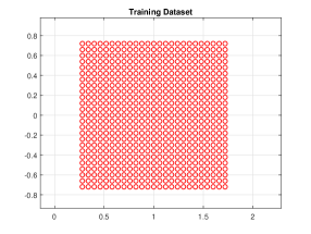
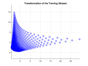
Figure 1. On the left we report the grid of points $\{x^{1},\ldots,x^{M}\}$ where we have evaluated the diffeomorphism $\Psi:\mathbb{R}^{2}\to\mathbb{R}^{2}$ defined as in (8.3). The picture on the right represents the transformation of the training dataset through the diffeomorphism $\Psi$.

If we denote by $\mu$ the probability measure that charges uniformly the square and if we set $\mu_{M}:=\frac{1}{M}\sum_{j=1}^{M}\delta_{x^{j}}$, we obtain the following estimate

$$W_{1}(\mu_{M},\mu)\leq\frac{\sqrt{2}\ell}{2\sqrt{M}},$$

that can be used to compute the a priori estimate of the generalization error provided by (5.12). We use the $1-$Lipschitz loss function

$$a(x-y):=\sqrt{1+(x_{1}-y_{1})^{2}+(x_{2}-y_{2})^{2}}-1,$$

and we look for a minimizer of

$$\mathcal{F}^{M}(u):=\frac{1}{900}\sum_{j=1}^{900}a(\Phi_{u}(x^{j})-\Psi(x^{j}))+\frac{\beta}{2}||u||^{2}_{L^{2}},$$ (8.4)

where $\beta>0$ is the regularization hyper-parameter. In the training phase we use the same dataset for Algorithm 1 and Algorithm 2, and in both cases the initial guess of the control is $u\equiv 0$. Finally, the testing dataset has been generated by randomly sampling $300$ points using $\mu$, the uniform probability measure on the square. The value of the hyper-parameter $\nu$ is set equal to $20$. We first tried to approximate the diffeomorphism $\Psi$ using $h=2^{-4}$, resulting in $16$ inner layers. Hence, recalling that each building-block (8.2) has $8$ parameters, the corresponding ResNet has in total $128$ parameters. We tested different values of $\beta$, and we set $\mathrm{max}_{iter}=500$. The results obtained by Algorithm 1 and Algorithm 2 are reported in Table 1 and Table 2, respectively. We observe that in both algorithms the Lipschitz constant of the produced diffeomorpism grows as the hyper-parameter $\beta$ gets smaller, consistently with the theoretical intuition. As regards the testing error, we observe that it always remains reasonably close to the corresponding training error.

$\beta$	$L_{\Phi_{u}}$	Training error	Testing error
$10^{0}$	$1.19$	$3.8785$	$3.8173$
$10^{-1}$	$8.40$	$1.3143$	$1.2476$
$10^{-2}$	$9.32$	$1.1991$	$1.1451$
$10^{-3}$	$9.37$	$1.1852$	$1.1330$
$10^{-4}$	$9.37$	$1.1839$	$1.1318$

Table 1. ResNet 8.2, $16$ layers, $128$ parameters, Algorithm 1. Running time $\sim 160$ s.

$\beta$	$L_{\Phi_{u}}$	Training error	Testing error
$10^{0}$	$1.19$	$3.8749$	$3.8157$
$10^{-1}$	$8.40$	$1.3084$	$1.2455$
$10^{-2}$	$9.32$	$1.2014$	$1.1486$
$10^{-3}$	$9.33$	$1.1898$	$1.1387$
$10^{-4}$	$9.33$	$1.1898$	$1.1379$

Table 2. ResNet 8.2, $16$ layers, $128$ parameters, Algorithm 2. Running time $\sim 130$ s.

We report in Figure 2 the image of the approximation that achieves the best training and testing errors, namely Algorithm 1 with $\beta=10^{-4}$. As we may observe, the prediction is quite unsatisfactory, both on the training and on the testing data-sets. Finally, we report that the formula (5.12) correctly provides an upper bound to the testing error, even though it is too pessimistic to be of practical use.

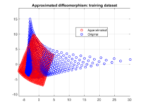
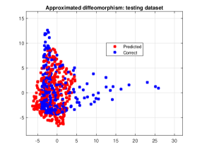
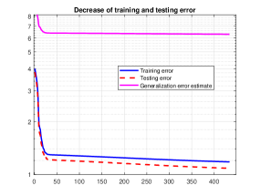
Figure 2. ResNet 8.2, 16 layers, Algorithm 1, $\beta=10^{-4}$. On the top-left we reported the transformation of the initial grid through the approximating diffeomorphism (red circles) and through the original one (blue circles). On the top-right, we plotted the prediction on the testing data-set provided by the approximating diffeomorphism (red crosses) and the correct values obtained through the original transformation (blue crosses). In both cases, the approximation obtained is unsatisfactory. At bottom we plotted the decrease of the training error and the testing error versus the number of iterations. Finally, the curve in magenta represents the estimate of the generalization error provided by (5.12).

In order to improve the quality of the approximation, a natural attempt consists in trying to increase the depth of the ResNet. Therefore, we repeated the experiments setting $h=2^{-5}$, that corresponds to $32$ layers. Recalling that the ResNet in exam has $8$ parameters per layer, the architecture has globally $256$ weights. The results are reported in Table 3 and Table 4. Unfortunately, despite doubling the depth of the ResNet, we do not observe any relevant improvement in the training nor in the testing error. Using the idea explained in Remark 3.9, instead of further increase the number of the layers, we try to enlarge the family of the controlled vector fields in the control system associated to the ResNet.

$\beta$	$L_{\Phi_{u}}$	Training error	Testing error
$10^{0}$	$1.19$	$3.8779$	$3.8168$
$10^{-1}$	$8.40$	$1.3074$	$1.2425$
$10^{-2}$	$9.26$	$1.2015$	$1.1477$
$10^{-3}$	$9.34$	$1.1860$	$1.1352$
$10^{-4}$	$9.34$	$1.1842$	$1.1332$

Table 3. ResNet 8.2, $32$ layers, $256$ parameters, Algorithm 1. Running time $\sim 320$ s.

$\beta$	$L_{\Phi_{u}}$	Training error	Testing error
$10^{0}$	$1.19$	$3.8739$	$3.8148$
$10^{-1}$	$8.35$	$1.3085$	$1.2449$
$10^{-2}$	$9.23$	$1.2075$	$1.1538$
$10^{-3}$	$9.26$	$1.1931$	$1.1416$
$10^{-4}$	$9.26$	$1.1918$	$1.1404$

Table 4. ResNet 8.2, $32$ layers, $256$ parameters, Algorithm 2. Running time $\sim 260$ s.

8.2. Enlarged family of controlled fields

Using the ideas expressed in Remark 3.9, we enrich the family of the controlled fields. In particular, in addition to the fields considered above, we include the following ones:

$$G^{1,1}_{1}:=x_{1}^{2}e^{-\frac{1}{2\nu}|x|^{2}}\frac{\partial}{\partial x_{1}},\quad G^{1,2}_{1}:=x_{1}x_{2}e^{-\frac{1}{2\nu}|x|^{2}}\frac{\partial}{\partial x_{1}},\quad G^{2,2}_{1}:=x_{2}^{2}e^{-\frac{1}{2\nu}|x|^{2}}\frac{\partial}{\partial x_{1}},$$

$$G^{1,1}_{2}:=x_{1}^{2}e^{-\frac{1}{2\nu}|x|^{2}}\frac{\partial}{\partial x_{2}},\quad G^{1,2}_{2}:=x_{1}x_{2}e^{-\frac{1}{2\nu}|x|^{2}}\frac{\partial}{\partial x_{2}},\quad G^{2,2}_{2}:=x_{2}^{2}e^{-\frac{1}{2\nu}|x|^{2}}\frac{\partial}{\partial x_{2}}.$$

Therefore, the resulting linear-control system on the time interval $[0,1]$ has the form

$$\dot{x}=\left(\begin{matrix}u_{1}\\ u_{2}\end{matrix}\right) +e^{-\frac{1}{2\nu}|x|^{2}}\left(\begin{matrix}u_{1}^{\prime}\\ u_{2}^{\prime}\end{matrix}\right)+\left(\begin{matrix}u_{1}^{1}&u^{2}_{1}\\ u_{2}^{1}&u_{2}^{2}\end{matrix}\right)\left(\begin{matrix}x_{1}\\ x_{2}\end{matrix}\right)$$

$$\qquad+e^{-\frac{1}{2\nu}|x|^{2}}\left(\begin{matrix}u_{1}^{1,1}x_{1}^{2}+u_{1}^{1,2}x_{1}x_{2}+u_{1}^{2,2}x_{2}^{2}\\ u_{2}^{1,1}x_{1}^{2}+u_{2}^{1,2}x_{1}x_{2}+u_{2}^{2,2}x_{2}^{2}\end{matrix}\right),$$

while the building blocks of the corresponding ResNet have the following expression:

$$\Phi_{k}(x)=x+h \left[\left(\begin{matrix}u_{1}\\ u_{2}\end{matrix}\right)+e^{-\frac{1}{2\nu}|x|^{2}}\left(\begin{matrix}u_{1}^{\prime}\\ u_{2}^{\prime}\end{matrix}\right)+\left(\begin{matrix}u_{1}^{1}&u^{2}_{1}\\ u_{2}^{1}&u_{2}^{2}\end{matrix}\right)\left(\begin{matrix}x_{1}\\ x_{2}\end{matrix}\right)\right.$$ (8.5)

$$\left.\qquad+e^{-\frac{1}{2\nu}|x|^{2}}\left(\begin{matrix}u_{1}^{1,1}x_{1}^{2}+u_{1}^{1,2}x_{1}x_{2}+u_{1}^{2,2}x_{2}^{2}\\ u_{2}^{1,1}x_{1}^{2}+u_{2}^{1,2}x_{1}x_{2}+u_{2}^{2,2}x_{2}^{2}\end{matrix}\right)\right]$$ (8.6)

for $k=1,\ldots,N$, where $h=\frac{1}{N}$ is the discretization step-size and $N$ is the number of layers of the ResNet. We observe that each building block has $14$ parameters.

As before, we set $\nu=20$, $\mathrm{max}_{iter}=500$ and we considered $h=2^{-4}$, resulting in a ResNet with $16$ layers and with total number of weights equal to $224$. We used the same training data-set as above, namely the grid of points and the corresponding image trough $\Psi$ depicted in Figure 1. We trained the network using both Algorithm 1 and Algorithm 2. The results are collected in Table 5 and Table 6, respectively. Once again, we observe that the Lipschitz constant of the approximating diffeomorphisms grows as $\beta$ is reduced. In this case, with both algorithms, the training and testing errors are much lower if compared with the best case of the ResNet 8.2. We insist on the fact that in the present case the ResNet 8.5-8.6 has in total $224$ parameters divided into $16$ layers, and it overperforms the ResNet 8.2 with $256$ parameters divided into $32$ layers. We report in Figure 3 the approximation produced by Algorithm 1 with $\beta=10^{-3}$. In this case the approximation provided is very satisfactory, and we observe that it is better in the area where more observations are available. Finally, also in this case the estimate on the expected generalization error (5.12) provides an upper bound for the testing error, but at the current state it is too coarse to be of practical use.

$\beta$	$L_{\Phi_{u}}$	Training error	Testing error
$10^{0}$	$10.14$	$2.3791$	$2.3036$
$10^{-1}$	$13.84$	$0.1809$	$0.2314$
$10^{-2}$	$15.64$	$0.1290$	$0.1784$
$10^{-3}$	$15.83$	$0.1254$	$0.1747$
$10^{-4}$	$15.86$	$0.1257$	$0.1751$

Table 5. ResNet 8.5-8.6, $16$ layers, $224$ parameters, Algorithm 1. Running time $\sim 320$ s.

$\beta$	$L_{\Phi_{u}}$	Training error	Testing error
$10^{0}$	$10.78$	$2.3638$	$2.3910$
$10^{-1}$	$14.32$	$0.1921$	$0.2422$
$10^{-2}$	$15.43$	$0.1887$	$0.2347$
$10^{-3}$	$15.56$	$0.2260$	$0.2719$
$10^{-4}$	$15.59$	$0.2127$	$0.2564$

Table 6. ResNet 8.5-8.6, $16$ layers, $224$ parameters, Algorithm 2. Running time $\sim 310$ s.

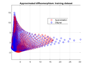
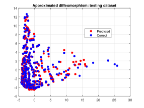
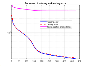
Figure 3. ResNet 8.5-8.6, 16 layers, Algorithm 1, $\beta=10^{-3}$. On the top-left we reported the transformation of the initial grid through the approximating diffeomorphism (red circles) and through the original one (blue circles). On the top-right, we plotted the prediction on the testing data-set provided by the approximating diffeomorphism (red crosses) and the correct values obtained through the original transformation (blue crosses). In both cases, the approximation obtained is good, and we observe that it is better where we have more data density. At bottom we plotted the decrease of the training error and the testing error versus the number of iterations. Finally, the curve in magenta represents the estimate of the generalization error provided by (5.12).

Conclusions

In this paper we have derived a Deep Learning architecture for a Residual Neural Network starting from a control system. Even though this approach has already been undertaken in some recent works (see [14], [16], [19], [8], [10]), the original aspect of our contribution lies in the fact that the control system considered here is linear in the control variables. In spite of this apparent simplicity, the flows generated by these control systems (under a suitable assumption on the controlled vector fields) can approximate with arbitrary precision on compact sets any diffeomorphism diffeotopic to the identity (see [4], [5]). Moreover, the linearity in the control variables simplifies the implementation and the computational effort required in the training procedure. Indeed, when the parameters are learned via a Maximum-Principle approach, the maximization of the Hamiltonian function is typically highly time-consuming if the control system is non-linear in the control variables. In the paper we propose two training procedure. The first one consists in projecting onto a finite-dimensional space the gradient flow associated to a proper Optimal Control problem. The second procedure relies on an iterative method for the solution of Optimal Control problems based on Pontryagin Maximum Principle. We have tested the learning algorithms on a diffeomorphism approximation problem in $\mathbb{R}^{2}$, obtaining interesting results. We plan to investigate in future work the performances of this kind of Neural Networks in other learning tasks, such as classification.

Acknowledgments

The Author acknowledges partial support from INDAM-GNAMPA. The Author wants to thank Prof. A. Agrachev and Prof. A. Sarychev for encouraging and for the helpful discussions. The Author is grateful to an anonymous referee for the invaluable suggestions that contributed to improve the quality of the paper.

(A. Scagliotti) Scuola Internazionale Superiore di Studi Avanzati, Trieste, Italy.
Email address: ascaglio@sissa.it

References

- [1] A.A. Agrachev, Y.L. Sachkov. Control Theory from the Geometric Viewpoint. Springer-Verlag Berlin Heidelberg (2004).
- [2] A.A. Agrachev, D. Barilari, U. Boscain. A Comprehensive Introduction to Sub-Riemannian Geometry. Cambridge University Press (2019).
- [3] A.A. Agrachev, Y.M. Baryshnikov, A.V. Sarychev. Ensemble controllability by Lie algebraic methods. ESAIM: Cont., Opt. and Calc. Var., 22:921–938 (2016).
- [4] A.A. Agrachev, A.V. Sarychev. Control in the Spaces of Ensembles of Points. SIAM J. Control Optim., 58(3):1579–1596 (2020).
- [5] A.A. Agrachev, A.V. Sarychev. Control on the Manifolds of Mappings with a View to the Deep Learning. J. Dyn. Control Syst., (2021).
- [6] L. Ambrosio, N. Gigli, G. Savaré. Gradient flows in metric spaces and in the space of probability measures. Springer Science & Business Media (2008).
- [7] Y. Bengio, P. Simard, P. Frasconi. Learning long-term dependencies with gradient descent is difficult. IEEE Trans. Neural Netw., 5(2):157–166 (1994).
- [8] M. Benning, E. Celledoni, M.J. Erhardt, B. Owren, C.B. Schönlieb. Deep learning as optimal control problems: Models and numerical methods. J. Comput. Dyn., 6(2):171–198 (2019).
- [9] M. Bongini, M. Fornasier, F. Rossi, F. Solombrino. Mean-field Pontryagin Maximum Principle, J. Optim. Theory Appl., 175(1):1–38 (2017).
- [10] B. Bonnet, C. Cipriani, M. Fornasier, H. Huang. A measure theoretical approach to the Mean-field Maximum Principle for training NeurODEs. Preprint arXiv:2107.08707 (2021).
- [11] F.L. Chernousko, A.A. Lyubushin. Method of successive approximations for solution of optimal control problems. Optim. Control Appl. Methods, 3(2):101-114 (1982).
- [12] E. Çinlar. Probability and Stochastics. Springer-Verlag, New York (2010).
- [13] G. Dal Maso. An Introduction to -convergence. Birkhäuser, Boston, MA (1993).
- [14] W. E. A Proposal on Machine Learning via Dynamical Systems. Commun. Math. Stat., 5(1):1–11 (2017).
- [15] I. Goodfellow, Y. Bengio, A. Courville. Deep Learning. MIT Press (2016).
- [16] E. Haber, L. Ruthotto. Stable architectures for deep neural networks. Inverse Problems, 34(1) (2017).
- [17] K. He, J. Sun. Convolutional neural networks at constrained time cost. 2015 IEEE Conference on Computer Vision and Pattern Recognition (CVPR), pp. 5353–5360 (2015).
- [18] K. He, X. Zhang, S. Ren, J. Sun. Deep residual learning for image recognition. Proceedings of the IEEE conference on computer vision and pattern recognition, pp. 770–778 (2016).
- [19] Q. Li, L. Chen, C. Tai, W. E. Maximum Principle Based Algorithms for Deep Learning. J. Mach. Learn. Res., 18(1):5998–6026 (2017).
- [20] M. Marchi, B. Gharesifard, P. Tabuada. Training deep residual networks for uniform approximation guarantees. PMLR, 144:677–688 (2021).
- [21] A.V. Pukhlikov. Optimal Control of Distributions. Comput. Math. Model., 15:223–256 (2004).
- [22] Y. Sakawa, Y. Shindo. On global convergence of an algorithm for optimal control. IEEE Trans. Automat. Contr., 25(6):1149–1153 (1980).
- [23] A. Scagliotti. A gradient flow equation for optimal control problems with end-point cost. J. Dyn. Control Syst., to appear (2022).
- [24] P. Tabuada, B. Gharesifard. Universal Approximation Power of Deep Neural Networks via Nonlinear Control Theory. Preprint arXiv:007.06007 (2020).
- [25] M. Thorpe, Y. van Gennip. Deep Limits of Residual Neural Networks. Preprint arXiv:1810.11741 (2018).