Heteroclinic Cycles of a Symmetric May-Leonard Competition Model with Seasonal Succession

Abstract

In this paper, we are concerned with the stability of heteroclinic cycles of the symmetric May-Leonard competition model with seasonal succession. Sufficient conditions for stability of heteroclinic cycles are obtained. Meanwhile, we present the explicit expression of the carrying simplex in a special case. By taking $\varphi$ as the switching strategy parameter for a given example, the bifurcation of stability of the heteroclinic cycle is investigated. We also find that there are rich dynamics (including nontrivial periodic solutions, invariant closed curves and heteroclinic cycles) for such a new system via numerical simulation. Biologically, the result is interesting as a caricature of the complexities that seasonal succession can introduce into the classical May-Leonard competitive model.

Keywords: May-Leonard competitive model, Seasonal succession, Heteroclinic Cycles, Carrying simplex, Bifurcation

AMS Subject Classification (2020): 34C12, 34C25, 34D23, 37C65, 92D25

1 Introduction

Lotka-Volterra competition is modeled by a system of differential equations describing the competition between two or more species that compete for the same resources or habitat. There have been extensive studies and applications of Lotka-Volterra competition models (see [3, 10, 16, 17, 23, 24, 29, 35]). In particular, May and Leonard [25] focused on the case that all three competing species have the same intrinsic growth rates and the three species compete in the “rock-scissors-paper” manner, which is modeled by the following form

$$\begin{cases}\frac{dx_{1}}{dt}=x_{1}(1-x_{1}-\alpha x_{2}-\beta x_{3}),\\ \frac{dx_{2}}{dt}=x_{2}(1-\beta x_{1}-x_{2}-\alpha x_{3}),\\ \frac{dx_{3}}{dt}=x_{3}(1-\alpha x_{1}-\beta x_{2}-x_{3}),\\ (x_{1}(0),x_{2}(0),x_{3}(0))=x^{0}\in R_{+}^{3},\end{cases}$$ (1.1)

where $0<\alpha<1<\beta$ and $\alpha+\beta>2$. They found numerically that system (1.1) exhibits a general class of solutions with non-periodic oscillations of bounded amplitude but ever-increasing cycle time; asymptotically, the system cycles from being composed almost wholly of population 1, to almost wholly 2, to almost wholly 3, back to almost wholly 1, etc. The rigorous proof was attributed to Schuster, Sigmund and Wolf [30]. This interesting cyclical fluctuation phenomenon was later known as “May-Leonard phenomenon”. In [2], Chi, Hsu and Wu obtained a complete classification for the global dynamics of the asymmetric May-Leonard competition model, and exhibited the May-Leonard phenomenon under certain conditions. For discrete-time cases, Roeger and Allen [27] studied two discrete-time models applicable to three competing plant species and proved that there also exist similar dynamics to system (1.1). Recently, Jiang et al. investigated three-dimensional Kolmogorov competitive systems admitting a carrying simplex, and derived that these systems have heteroclinic cycles (see [12, 13, 14, 16]), which implies that May-Leonard phenomenon happens and greatly enriches existing results of heteroclinic cycles for competitive systems. Furthermore, Jiang, Niu and Wang [15] analyzed the effects of heteroclinic cycles and the interplay of heteroclinic attractors or repellers on the boundary of the carrying simplices for three-dimensional competitive maps. For more results of heteroclinic cycles, we refer to [5, 19, 20, 4, 11, 6, 7] and references therein.

On the other hand, alternation of seasons is a very common phenomenon in nature. The alternations may be fast (e.g., daily light change, Litchman and Klausmeier [22]), intermediate (e.g., tidal cycles and annual seasons, DeAngelis et al.[21]), or slow (e.g., EI Nino events). Due to the seasonal alternation, populations experience a periodic external environment such as temperature, rainfall, humidity and wind. One impressive example occurs in phytoplankton and zooplankton of the temperate lakes, where the species grow during the warmer months and die off or form resting stages in the winter. Such phenomenon is called seasonal succession in Sommer et al.[31]. In [8], Hu and Tessier’s study on competitive interactions of two Daphnia species in Gull Lake suggested that the strength of interspecific and intraspecific competition varied with season. This seasonal shift in the nature of competitive interactions provides an explanation for seasonal succession in this Daphnia assemblage.

In fact, seasonal forcing is a major cause of nonequilibrium dynamics. It has been a fascinating subject for ecologists and mathematicians to explore the modeling of nonequilibrium dynamics by means of seasonal succession. As early as 1974, Koch [17] considered a two species competition model in a seasonal environment, where good and bad seasons alternate. In the good season from spring to autumn, the species follow Lotka-Volterra competition interaction. While, the species reduce by some constant factors due to adverse conditions in the bad season from autumn to spring through winter. This research stated that although a chance fluctuation may affect the relative extent of growth of the two species in a particular year leading to a change in the input ratio of populations the following spring, under fairly general circumstances, this can affect the growth cycle of the two species in just the right way to return the system towards its original cycle so as to permit stable. Litchman and Klausmeier [22] analyzed a competition model of two species for a single nutrient under fluctuating light with seasonal succession in the chemostat. Later, Klausmeier [18] described a novel approach to modeling seasonally forced food webs (called successional state dynamics-SSD). The approach treats succession as a series of state transitions driven by both the internal dynamics of species interactions and external forcing. It is applicable to communities where species dynamics are fast relative to the external forcing, such as plankton and other microbes, diseases, and some insect communities. By applying this approach to the classical Rosenzweig-MacArthur predator-prey model, he found numerically that the forced dynamics are more complicated, showing multiannual cycles or apparent chaos. In Steiner et al.[28], the SSD modeling approach was then employed to generate analytical predictions of the effects of altered seasonality on species persistence and the timing of community state transitions, which highlighted the utility of the SSD modeling approach as a framework for predicting the effects of altered seasonality on the structure and dynamics of multitrophic communities. In theory, Hsu and Zhao [10] first studied the global dynamics of a two-species Lotka-Volterra two-species competition model with seasonal succession and obtained a complete classification for the global dynamics via the theory of monotone dynamical systems. Xiao [34] discussed the effect of the seasonal harvesting on the survival of the population for a class of population model with seasonal constant-yield harvesting. In recent years, SSD modeling approach has attracted considerable attention in theoretical ecology, see [35, 32, 1, 9] and references therein. Although the seasonal succession model looks like a periodic system, its coefficients are discontinuous and periodic in time $t$. Many known results on periodic systems with continuous periodic coefficients are not applicable to these models (e.g. Cushing [3]). Besides, it is still challenging to understand the mechanisms of seasonal succession and their impacts on the dynamics of communities and ecosystems.

Motivated by the SSD modeling approach in Klausmeier [18], we propose a three-dimensional May-Leonard competition model with seasonal succession as follows:

$$\begin{cases}\frac{dx_{i}}{dt}=-\lambda_{i}x_{i},\qquad\quad\qquad\ m\omega\leq t\leq m\omega+(1-\varphi)\omega,\quad i=1,2,3,\\ \frac{dx_{1}}{dt}=x_{1}(1-x_{1}-\alpha x_{2}-\beta x_{3}),\ m\omega+(1-\varphi)\omega\leq t\leq(m+1)\omega,\\ \frac{dx_{2}}{dt}=x_{2}(1-\beta x_{1}-x_{2}-\alpha x_{3}),\ m\omega+(1-\varphi)\omega\leq t\leq(m+1)\omega,\\ \frac{dx_{3}}{dt}=x_{3}(1-\alpha x_{1}-\beta x_{2}-x_{3}),\ \ m\omega+(1-\varphi)\omega\leq t\leq(m+1)\omega,\\ \big{(}x_{1}(0),x_{2}(0),x_{3}(0)\big{)}=x^{0}\in\mathbb{R}^{3}_{+},\quad\qquad\ m=0,1,2\dots\\ \end{cases}$$ (1.2)

where $m\in\mathbb{Z_{+}}$, $\varphi\in[0,1]$, $\omega$, $\alpha$, $\beta$, $\lambda_{i}\ (i=1,2,3)$ are all positive constants.

Clearly, if $\varphi=0$, then the system (1.2) become the following decoupling form

$$\begin{cases}\frac{dx_{i}}{dt}=-\lambda_{i}x_{i},\qquad\quad i=1,2,3,\\ \big{(}x_{1}(0),x_{2}(0),x_{3}(0)\big{)}=x^{0}\in\mathbb{R}^{3}_{+}.\\ \end{cases}$$ (1.3)

While, if $\varphi=1$, system (1.2) turns out to be the symmetric May-Leonard competition model (1.1).

From system (1.2), one can see that it is a time-periodic system in a seasonal environment. Overall period is $\omega$, and $\varphi$ represents the switching proportion of a period between two subsystems (1.3) and (1.1). Biologically, $\varphi$ is used to describe the proportion of the period in the good season in which the species follow system (1.1), while $(1-\varphi)$ stands for the proportion of the period in the bad season in which the species die exponentially according to system (1.3).

It is not difficult to see that system (1.2) admits a unique nonnegative global solution $x(t,x^{0})$ on $[0,+\infty)$ for any $x^{0}\in\mathbb{R}^{3}_{+}$. Since system (1.2) is $\omega$-periodic, we only consider the Poincar$\acute{\rm e}$ map $S$ on $\mathbb{R}^{3}_{+}$, that is, $S(x^{0})=x(\omega,x^{0})$ for any $x^{0}\in\mathbb{R}_{+}^{3}$. Due to system (1.3), let us first define a linear map $L$ by

$$L(x_{1},x_{2},x_{3})=(e^{-\lambda_{1}(1-\varphi)\omega}x_{1},e^{-\lambda_{2}(1-\varphi)\omega}x_{2},e^{-\lambda_{3}(1-\varphi)\omega}x_{3}),\ \forall\ (x_{1},x_{2},x_{3})\in\mathbb{R}^{3}_{+}.$$

We also let $\{Q_{t}\}_{t\geq 0}$ represent the solution flow associated with the symmetric May-Leonard competition system (1.1). Then, we have

$$S(x^{0})=Q_{\varphi\omega}(Lx^{0}),\qquad\forall x^{0}\in\mathbb{R}^{3}_{+},\qquad{\rm{i.e.,}}\qquad S=Q_{\varphi\omega}\circ L.$$

Hence, it suffices to investigate the dynamics of the discrete-time system $\{S^{n}\}_{n\geq 0}$. However, compared to the concrete discrete-time competitive maps discussed in [4, 13, 14, 16, 6, 7], there is no explicit expression of the Poincar$\acute{\rm e}$ map $S$ for system (1.2). This makes the research much more difficult and complicated on the dynamics of system (1.2).

The main aim of this paper is to establish the stability criterion of heteroclinic cycles for system (1.2), as well as its application on a given system (4.1). More precisely, it is proved that system (1.2) admits a heteroclinic cycle $\Gamma$ connecting the three axial fixed points $R_{i}(i=1,2,3)$ via the theory of the carrying simplex (see Theorem 3.6). Based on this, sufficient conditions for stability of the heteroclinic cycle are obtained (see Theorem 3.7). In particular, when $\lambda_{1}=\lambda_{2}=\lambda_{3}$ and $\alpha+\beta\neq 2$, we show that system (1.2) inherits stability properties of the heteroclinic cycle of classical May-Leonard system (1.1). Meanwhile, we also present the explicit expression of the carrying simplex in the case that $\alpha+\beta=2$ (see Corollary 3.8). For a given system (4.1), the critical value of the existence of the heteroclinic cycle is determined (see Theorem 4.1). By applying the stability criterion for system (1.2) to the given system (4.1), we obtain the stability branches of the heteroclinic cycle for such a system (see Theorem 4.2). Moreover, the branch graph of stability is demonstrated in Figure 3. By numerical simulation, we find that there are rich dynamics for the system as $\varphi$ varies. To be more explicit, when $\varphi$ varies in $[0,1]$, system (4.1) enjoys different dynamic features: the orbit emanating from initial value $x^{0}=(0.5,0.6,0.4)$ for the Poincar$\acute{\rm e}$ map $\tilde{S}$ tends to the heteroclinic cycle $\tilde{\Gamma}$(see Figure 4) $\rightarrow$ invariant closed curves (see Figure 6 and Figure 7) $\rightarrow$ the positive fixed point (see Figure 8-12) $\rightarrow$ the interior fixed point of coordinate plane $\{x_{2}=0\}$ (see Figure 13) $\rightarrow$ the interior fixed point of $x_{1}$-axis (see Figure 14) $\rightarrow$ the interior fixed point of the coordinate plane $\{x_{3}=0\}$ (see Figure 15) $\rightarrow$ the interior fixed point of $x_{2}$-axis (see Figure 16) $\rightarrow$ the trivial fixed point $O$ (see Figure 17). From these numerical examples, one can see that the dynamic features and patterns generated by system (4.1) are much richer , which are different from concrete discrete-time competitive maps analyzed in [6, 7, 13, 14].

The paper is organized as follows. In section 2, we introduce some notations and relevant definitions. Section 3 is devoted to analyze the existence and stability of heteroclinic cycles of system (1.2). We investigate the stability branches of the heteroclinic cycle for a given system (4.1) and present the branch graph of stability in Section 4. Furthermore, we provide some numerical simulations to exhibit rich dynamics for system (4.1). This paper ends with a discussion in Section 5.

2 Notations and Definitions

Throughout this paper, let $Z_{+}$ denote the set of nonnegative integers. We use $\mathbb{R}^{n}_{+}$ to define the nonnegative cone $\mathbb{R}^{n}_{+}:=\{x\in\mathbb{R}^{n}:x_{i}\geq 0,\ i=1,\cdots,n\}$. Let $X\subseteq\mathbb{R}^{n}_{+}$ and $S:X\rightarrow X$ be a continuous map. The orbit of a state $x$ for $S$ is $\gamma(x)=\{S^{n}(x)$, $n\in\mathbb{Z}_{+}\}$. A fixed point $x$ of $S$ is a point $x\in X$ such that $S(x)=x$. A point $y\in X$ is called a $k$-periodic point of $S$ if there exists some positive integer $k>1$, such that $S^{k}(y)=y$ and $S^{m}(y)\neq y$ for every positive integer $m<k$. The $k$-periodic orbit of the $k$-periodic point $y$, $\gamma(y)=\{y$, $S(y)$, $S^{2}(y)$, $...$, $S^{k-1}(y)\}$, is often called a periodic orbit for short. The $\omega$-limit set of $x$ is defined by $\omega(x)=\{y\in\mathbb{R}_{+}^{n}:S^{n_{k}}x\rightarrow y\ (k\rightarrow\infty)\ {\rm for\ some\ sequence}\ n_{k}\rightarrow+\infty\ {\rm in}\ \mathbb{Z}_{+}\}$. If the orbit of a state $x$ for $S^{-1}$ exists, then the $\alpha$-limit set of $x$ is denoted by $\alpha(x)=\{y\in\mathbb{R}_{+}^{n}:S^{-n_{k}}x\rightarrow y\ (k\rightarrow\infty)\ {\rm for\ some\ sequence}\ n_{k}\rightarrow+\infty\ {\rm in}\ \mathbb{Z}_{+}\}$.

A set $V\subseteq X$ is called positively invariant under $S$ if $SV\subseteq V$, and invariant if $SV=V$. We call that a nonempty compact positively invariant subset $V$ repels for $S$ if there exists a neighborhood $U$ of $V$ such that given any $x\in X\setminus V$ there is a $k_{0}(x)$ such that $S^{k}x\in U^{c}$ (the complement of $U$) for $k\geq k_{0}(x)$, and $V$ is said to be an attractor for $S$, if there exists a neighborhood $U$ of $V$, such that $\lim\limits_{k\rightarrow+\infty}d(S^{k}x,V)=0$ uniformly in $x\in U$, where $d(\cdot,\cdot)$ is the metric for $X$; $V$ is referred to as a global attractor for $S$, if for any bounded set $U\subseteq X$, $\lim\limits_{k\rightarrow+\infty}d(S^{k}x,V)=0$ uniformly in $x\in U$. Note that if the orbit $\gamma(x)$ of $x$ has compact closure, $\omega(x)$ is nonempty, compact and invariant. If $S$ is a differentiable map, we write $DS(x)$ as the Jacobian matrix of $S$ at the point $x$ and the spectral radius of $DS(x)$ is denoted by $r(DS(x))$. For an $n\times n$ matrix $A$, we write $A\geq 0$ iff $A$ is a nonnegative matrix (i.e., all the entries are nonnegative) and $A\gg 0$ iff $A$ is a positive matrix (i.e., all the entries are positive).

A map $S$ is said to be competitive in $\mathbb{R}_{+}^{n}$, if $x,y\in\mathbb{R}_{+}^{n}$ and $S(x)<S(y)$, then $x<y$. Furthermore, $S$ is called strongly competitive in $\mathbb{R}_{+}^{n}$, if $S(x)<S(y)$ then $x\ll y$.

A carrying simplex for the periodic map $S$ is a subset $\Sigma\subset\mathbb{R}_{+}^{n}\backslash\{0\}$ with the following properties (see [33, Theorem 11]):
$\rm(P1)$ $\Sigma$ is compact, invariant and unordered;
$\rm(P2)$ $\Sigma$ is homeomorphic via radial projection to the $(n-1)$-dim standard probability simplex $\Delta^{n-1}:=\{x\in\mathbb{R}_{+}^{n}|$ $\Sigma_{i}x_{i}=1\}$;
$\rm(P3)$ $\forall\ x\in\mathbb{R}_{+}^{n}\backslash\{0\}$, there exists some $y\in\Sigma$ such that $\lim\limits_{n\rightarrow\infty}|S^{n}x-S^{n}y|=0$.

3 Heteroclinic cycle

For system (1.2), it is clear that $O:=(0,0,0)$ is a trivial fixed point of the Poincar$\acute{\rm e}$ map $S$. Denote $h_{i}:=(\varphi-\lambda_{i}(1-\varphi))\omega,i=1,2,3.$ By Hsu and Zhao [10, Lemma 2.1], if $h_{i}>0$ $(i=1,2,3)$, then $S$ has three axial fixed points, written as $R_{1}:=(x_{1}^{*},0,0)$, $R_{2}:=(0,x_{2}^{*},0)$ and $R_{3}:=(0,0,x_{3}^{*})$. Besides, there are three planar fixed points for $S$ in three coordinate planes under appropriate conditions (see [10, Theorem 2.2-2.4] or [26, Theorem 3.6]). First, we provide the existence result of carrying simplex for system (1.2).

Lemma 3.1.

(The existence of the carrying simplex) Assume that $h_{i}>0,i=1,2,3$. Let $S:\mathbb{R}_{+}^{3}\rightarrow\mathbb{R}_{+}^{3}$ be the Poincar$\acute{e}$ map induced by system (1.2). Then, system (1.2) admits a two-dimensional carrying simplex $\Sigma$ which attracts every nontrivial orbit in $\mathbb{R}_{+}^{3}$.

Proof.

The statement is a result of Niu et al. [26, Theorem 2.3] for $n=3$, $b_{i}=a_{ii}=1\ (i=1,2,3)$, $a_{12}=a_{23}=a_{31}=\alpha$ and $a_{32}=a_{21}=a_{13}=\beta$, where $b_{i},a_{ij},i,j=1,2,3$ are defined in [26]. ∎

By the stability analysis of equilibria, we have

Lemma 3.2.

(Stability of the fixed point $O$) Given system (1.2), then

1. If $h_{i}<0$ $(i=1,2,3)$, then $O$ is an asymptotically stable fixed point of $S$.

2. If one of three values $h_{1},h_{2}$ and $h_{3}$ is greater than $0$, then $O$ is an unstable fixed point of $S$. In particular, if $h_{i}>0$ $(i=1,2,3)$, then $O$ is a hyperbolic repeller.

Proof.

Let $f(x)=(f_{1},f_{2},f_{3})^{T}$, where

$$\left\{\begin{array}[]{ll}\displaystyle f_{1}=x_{1}(1-x_{1}-\alpha x_{2}-\beta x_{3}),\\ \displaystyle f_{2}=x_{2}(1-\beta x_{1}-x_{2}-\alpha x_{3}),\\ \displaystyle f_{3}=x_{3}(1-\alpha x_{1}-\beta x_{2}-x_{3}).\\ \end{array}\right.$$

Then, $Df(x)=$

$$\left(\begin{matrix}1-2x_{1}-\alpha x_{2}-\beta x_{3}&-\alpha x_{1}&-\beta x_{1}\\ -\beta x_{2}&1-2x_{2}-\beta x_{1}-\alpha x_{3}&-\alpha x_{2}\\ -\alpha x_{3}&-\beta x_{3}&1-2x_{3}-\alpha x_{1}-\beta x_{2}\end{matrix}\right).$$

For simplicity, we denote $u(t,x):=Q_{t}(x)$ and $V(t,x):=D_{x}u(t,x)=D_{x}Q_{t}(x)$, then $S(x)=Q_{\varphi\omega}(Lx)=u(\varphi\omega,Lx)$, and hence,

$$DS(x) =D(Q_{\varphi\omega}(Lx))\cdot D(Lx)$$

$$=V(\varphi\omega,Lx)\cdot D(Lx)$$

$$=V(\varphi\omega,Lx)\cdot{\rm diag}\big{(}{e^{-\lambda_{1}(1-\varphi)\omega}},{e^{-\lambda_{2}(1-\varphi)\omega}},{e^{-\lambda_{3}(1-\varphi)\omega}}\big{)}.$$

Note that $V(t,x)$ satisfies

$$\frac{dV(t)}{dt}=Df(u(t,x))V(t),\quad V(0)=I.$$

Taking $O=(0,0,0)$, we have $u(t,LO)=(0,0,0)$, then $Df(u(t,LO))={\rm diag}(1,1,1),$ and hence,

$$V(\varphi\omega,LO)={\rm diag}\Big{(}e^{\int_{0}^{\varphi\omega}1dt},e^{\int_{0}^{\varphi\omega}1dt},e^{\int_{0}^{\varphi\omega}1dt}\Big{)}.$$

By the expression of $S$, it follows that

$$DS(O)=\left(\begin{matrix}e^{(\varphi-\lambda_{1}(1-\varphi))\omega}&0&0\\ 0&e^{(\varphi-\lambda_{2}(1-\varphi))\omega}&0\\ 0&0&e^{(\varphi-\lambda_{3}(1-\varphi))\omega}\end{matrix}\right).$$

Consequently, the matrix $DS(O)$ has three positive eigenvalues $\mu_{1},\mu_{2}$ and $\mu_{3}$ given by

$$\mu_{1}=e^{h_{1}},\qquad\mu_{2}=e^{h_{2}}\quad{\rm and}\quad\mu_{3}=e^{h_{3}}.$$

Clearly, if $h_{i}<0$ $(i=1,2,3)$, then $\mu_{i}<1$, and hence $O$ is an asymptotically stable fixed point of $S$; if $h_{i}>0$, then $\mu_{i}>1,i=1,2,3$, which implies that $O$ is a hyperbolic repeller. We have proved the lemma. ∎

Lemma 3.3.

(Stability of the axial fixed point $R_{1}$) Given system (1.2), suppose that $h_{i}>0,$ $i=1,2,3$, then

1. If $h_{2}<\beta h_{1}$, $h_{3}<\alpha h_{1}$, then $R_{1}$ is an asymptotically stable fixed point of $S$.

2. If $h_{2}>\beta h_{1}$, $h_{3}>\alpha h_{1}$, then $R_{1}$ is a saddle point with two-dimensional unstable manifolds.

3. If $(h_{2}-\beta h_{1})(h_{3}-\alpha h_{1})<0$, then $R_{1}$ is a saddle point with one-dimensional unstable manifolds.

Proof.

Let $u(t,LR_{1}):=(u_{1}^{*}(t),0,0)$. By the proof of Lemma 3.2, it is easy to see that

$$Df(u(t,LR_{1}))=\left(\begin{matrix}1-2u_{1}^{*}(t)&-\alpha u_{1}^{*}(t)&-\beta u_{1}^{*}(t)\\ 0&1-\beta u_{1}^{*}(t)&0\\ 0&0&1-\alpha u_{1}^{*}(t)\end{matrix}\right).$$

Then,

$$V(\varphi\omega,LR_{1})=\left(\begin{matrix}e^{\int_{0}^{\varphi\omega}1-2u_{1}^{*}(t)dt}&*&*\\ 0&e^{\int_{0}^{\varphi\omega}1-\beta u_{1}^{*}(t)dt}&*\\ 0&0&e^{\int_{0}^{\varphi\omega}1-\alpha u_{1}^{*}(t)dt}\end{matrix}\right),$$

where $*$ represents unknown algebraic expressions. Observe that $u_{1}^{*}(t)$ satisfies

$$\frac{du_{1}^{*}(t)}{dt}=u_{1}^{*}(t)(1-u_{1}^{*}(t)).$$

Integrating the above equation for $t$ from $0$ to $\varphi\omega$, we have

$$\int_{0}^{\varphi\omega}u_{1}^{*}(t)dt=(\varphi-\lambda_{1}(1-\varphi))\omega,$$

and then, $DS(R_{1})=$

$$\left(\begin{matrix}e^{-(\varphi-\lambda_{1}(1-\varphi))\omega}&*&*\\ 0&e^{[(\varphi-\lambda_{2}(1-\varphi))-\beta(\varphi-\lambda_{1}(1-\varphi))]\omega}&*\\ 0&0&e^{[(\varphi-\lambda_{3}(1-\varphi))-\alpha(\varphi-\lambda_{1}(1-\varphi))]\omega}\end{matrix}\right).$$

Thus, the matrix $DS(R_{1})$ has three positive eigenvalues $\mu_{1},\mu_{2}$ and $\mu_{3}$ given by

$$\mu_{1}=e^{-h_{1}}<1,\qquad\mu_{2}=e^{h_{2}-\beta h_{1}}\quad{\rm and}\quad\mu_{3}=e^{h_{3}-\alpha h_{1}},$$

which implies that the statements (i)-(iii) are valid. The proof is completed. ∎

By symmetric arguments, we also have

Lemma 3.4.

(Stability of the axial fixed point $R_{2}$) Given system (1.2), suppose that $h_{i}>0,i=1,2,3$, then

1. If $h_{1}<\alpha h_{2}$, $h_{3}<\beta h_{2}$, then $R_{2}$ is an asymptotically stable fixed point of $S$.

2. If $h_{1}>\alpha h_{2}$, $h_{3}>\beta h_{2}$, then $R_{2}$ is a saddle point with two-dimensional unstable manifolds.

3. If $(h_{1}-\alpha h_{2})(h_{3}-\beta h_{2})<0$, then $R_{2}$ is a saddle point with one-dimensional unstable manifolds.

Lemma 3.5.

(Stability of the axial fixed point $R_{3}$) Given system (1.2), suppose that $h_{i}>0,i=1,2,3$, then

1. If $h_{1}<\beta h_{3}$, $h_{2}<\alpha h_{3}$, then $R_{3}$ is an asymptotically stable fixed point of $S$.

2. If $h_{1}>\beta h_{3}$, $h_{2}>\alpha h_{3}$, then $R_{3}$ is a saddle point with two-dimensional unstable manifolds.

3. If $(h_{1}-\beta h_{3})(h_{2}-\alpha h_{3})<0$, then $R_{3}$ is a saddle point with one-dimensional unstable manifolds.

For the sake of convenience, we introduce the following notation:
$(\tilde{H})$      $h_{2}<\beta h_{1},h_{1}>\alpha h_{2};\ h_{3}<\beta h_{2},h_{2}>\alpha h_{3};\ h_{1}<\beta h_{3},h_{3}>\alpha h_{1}.$
Moreover, we write $\vartheta$ as

$$\vartheta:=(h_{1}-\beta h_{3})(h_{2}-\beta h_{1})(h_{3}-\beta h_{2})+(h_{1}-\alpha h_{2})(h_{2}-\alpha h_{3})(h_{3}-\alpha h_{1}).$$

By the theory of the carrying simplex, we have

Theorem 3.6.

(The existence of the heteroclinic cycle) Suppose that the condition $(\tilde{H})$ holds and $h_{i}>0,i=1,2,3$, then system (1.2) admits a heteroclinic cycle $\Gamma$ ($=\partial\Sigma$) connecting the three axial fixed points $R_{1},R_{2}$ and $R_{3}$ , where $\partial\Sigma$ stands for the boundary of the carrying simplex $\Sigma$ (see Figure 1).

Proof.

By Lemma 3.1, system (1.2) admits a two-dimensional carrying simplex $\Sigma$. Furthermore, the intersection of $\Sigma$ with three coordinate planes is composed of three line segments connecting any two of $R_{i},i=1,2,3$. These three line segments are written as $\Gamma_{12},\Gamma_{23}$ and $\Gamma_{13}$, respectively. By the invariance of $\Sigma$, one can obtain that $\Gamma_{12},\Gamma_{23}$ and $\Gamma_{13}$ are invariant under the map $S$. In view of $h_{2}<\beta h_{1}$ and $h_{1}>\alpha h_{2}$, it follows from Niu et al. [26, Theorem 3.6(ii)] that there are no interior fixed points on $\Gamma_{12}$. Note that the restriction of $S$ to the segment $\Gamma_{12}$ must be a monotone one-dimensional map, all orbits on $\Gamma_{12}$ have one fixed point as the $\alpha$-limit set and the other as the $\omega$-limit set. Meanwhile, Niu et al. [26, Theorem 3.6(ii)] ensures that all orbits on $\Gamma_{12}$ take $R_{2}$ as the $\alpha$-limit set and $R_{1}$ as the $\omega$-limit set under the condition $(\tilde{H})$. By the cyclic symmetry, we also obtain that $\Gamma_{23}$ and $\Gamma_{13}$ have similar properties as $\Gamma_{12}$ under the condition $(\tilde{H})$. Define $\Gamma=\Gamma_{12}\cup\Gamma_{13}\cup\Gamma_{23}$, then $\Gamma=\partial\Sigma$. Furthermore, it is obvious that $\Gamma$ is a heteroclinic cycle connecting the three axial fixed points $R_{1},R_{2}$ and $R_{3}$, which forms the boundary $\partial\Sigma$ of $\Sigma$ (see Figure 1). We have thus proved the theorem. ∎

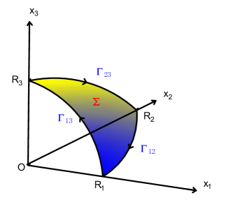
Figure 1: $\Gamma$ (Clockwise direction)

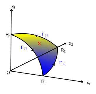
Figure 2: $\Gamma$ (Counter-clockwise direction)

Remark 3.1.

By modifying the proof of Theorem 3.6, it can easily be shown that if the condition $(\tilde{H})$ is revised as

$$h_{2}>\beta h_{1},h_{1}<\alpha h_{2};\ h_{3}>\beta h_{2},h_{2}<\alpha h_{3};\ h_{1}>\beta h_{3},h_{3}<\alpha h_{1},$$

then system (1.2) also admits a heteroclinic cycle connecting the three axial fixed points $R_{1},R_{2}$ and $R_{3}$, yet the arrows are reserved (see Figure 2).

Theorem 3.7.

(The stability of the heteroclinic cycle) Given system (1.2), suppose that the condition $(\tilde{H})$ holds and $h_{i}>0,i=1,2,3$, then

1. If $\vartheta>0$, then the heteroclinic cycle $\Gamma$ repels.

2. If $\vartheta<0$, then the heteroclinic cycle $\Gamma$ attracts.

Proof.

By the proof of Lemma 3.3 and Lemma 3.4-3.5, one can see that the eigenvalues of the matrices $DS(R_{1})$ and $DS(R_{3})$ along the $x_{2}$-axis direction are $e^{h_{2}-\beta h_{1}}$ and $e^{h_{2}-\alpha h_{3}}$, respectively; the eigenvalues of the matrices $DS(R_{1})$ and $DS(R_{2})$ along the $x_{3}$-axis direction are $e^{h_{3}-\alpha h_{1}}$ and $e^{h_{3}-\beta h_{2}}$, respectively; the eigenvalues of the matrices $DS(R_{2})$ and $DS(R_{3})$ along the $x_{1}$-axis direction are $e^{h_{1}-\alpha h_{2}}$ and $e^{h_{1}-\beta h_{3}}$, respectively. A simple calculation yields

$$\ln e^{h_{1}-\beta h_{3}}\cdot\ln e^{h_{2}-\beta h_{1}}\cdot\ln e^{h_{3}-\beta h_{2}}+\ln e^{h_{1}-\alpha h_{2}}\cdot\ln e^{h_{2}-\alpha h_{3}}\cdot\ln e^{h_{3}-\alpha h_{1}}$$

$$=(h_{1}-\beta h_{3})(h_{2}-\beta h_{1})(h_{3}-\beta h_{2})+(h_{1}-\alpha h_{2})(h_{2}-\alpha h_{3})(h_{3}-\alpha h_{1})=\vartheta.$$

Note that system (1.2) is a time-periodic Kolmogorov systems and the the Poincar$\rm\acute{e}$ map $S$ is $C^{1}$-diffeomorphism onto its image (see the proof of Theorem 2.3 in Niu et al. [26]), we can rewrite $S$ as:

$$S(x_{1},x_{2},x_{3})=(x_{1}G_{1}(x),x_{2}G_{2}(x),x_{3}G_{3}(x)),\quad x\in\mathbb{R}_{+}^{3},$$

where $G_{i}(x)=$ $\left\{\begin{array}[]{ll}\displaystyle\frac{S_{i}(x)}{x_{i}},\quad x_{i}\neq 0,\\ \displaystyle\frac{\partial S_{i}}{\partial x_{i}}(x),\quad x_{i}=0.\\ \end{array}\right.$ Then $S$ is considered as a Kolmogorov competitive map. According to Theorem 3 in Jiang, Niu and Wang [15], we can obtain that if $\vartheta>0$, then the heteroclinic cycle $\Gamma$ repels; if $\vartheta<0$, then the heteroclinic cycle $\Gamma$ attracts. Thus, we have completed the proof. ∎

In particular, when $\lambda_{1}=\lambda_{2}=\lambda_{3}$, we have

Corollary 3.8.

Given system (1.2), suppose that the condition $(\tilde{H})$ holds, $h_{i}>0\ (i=1,2,3)$, $\lambda_{1}=\lambda_{2}=\lambda_{3}=\lambda$ and $0<\alpha<1<\beta$ , then

1. If $\alpha+\beta<2$, then the heteroclinic cycle $\Gamma$ repels.

2. If $\alpha+\beta>2$, then the heteroclinic cycle $\Gamma$ attracts.

3. If $\alpha+\beta=2$, then the carrying simplex of system (1.2) is

   $$\Sigma=\{(x_{1},x_{2},x_{3})\in\mathbb{R}_{+}^{3}:x_{1}+x_{2}+x_{3}=\frac{1-e^{p-q}}{1-e^{-q}}\},$$

   where $p=\lambda(1-\varphi)\omega,\ q=\varphi\omega$. Furthermore, $P:=\frac{1-e^{p-q}}{3(1-e^{-q})}(1,1,1)$ is a positive fixed point of $S$.

Proof.

Since $\lambda_{1}=\lambda_{2}=\lambda_{3}$, it follows that $h_{1}=h_{2}=h_{3}$, and then,

$$\vartheta =h_{1}^{3}\big{(}(1-\beta)^{3}+(1-\alpha)^{3}\big{)}$$

$$=h_{1}^{3}\Big{(}\big{(}2-(\alpha+\beta)\big{)}\big{(}(1-\beta)^{2}+(\beta-1)(1-\alpha)+(1-\alpha)^{2}\big{)}\Big{)}.$$

Noticing that $0<\alpha<1<\beta,$ one can obtain that $\big{(}(1-\beta)^{2}+(\beta-1)(1-\alpha)+(1-\alpha)^{2}\big{)}>0.$ By $h_{i}>0\ (i=1,2,3)$, it is clear that if $\alpha+\beta<2$, then $\vartheta>0$; if $\alpha+\beta>2$, then $\vartheta<0$. This implies that the statements (i) and (ii) are true due to Theorem 3.7.

Finally, it remains to show that the statement (iii) holds. For this purpose, we firstly consider the one-dimensional case of system (1.2), that is,

$$\begin{cases}\frac{dx}{dt}=-\lambda x,\qquad\quad\;m\omega\leq t\leq m\omega+(1-\varphi)\omega,\\ \frac{dx}{dt}=x(1-x),\quad m\omega+(1-\varphi)\omega\leq t\leq(m+1)\omega,\\ x(0)=x_{0}\in\mathbb{R}_{+}.\end{cases}$$ (3.1)

Solving the equation $\frac{dx}{dt}=x(1-x)$ with the initial value $x^{0}\in\mathbb{R}_{+}$ yields

$$x(t,x^{0})=\frac{x^{0}}{x^{0}+(1-x^{0})e^{-t}},\qquad\forall\ t\geq 0,\ x^{0}\in\mathbb{R}_{+}.$$ (3.2)

Define the Poincar$\rm\acute{e}$ map of system (3.1),

$$\bar{S}(x_{0})=x(\omega,x_{0}),\ \forall\ x_{0}\in\mathbb{R}_{+}.$$

By Hsu and Zhao[10, Lemma 2.1], $\bar{S}$ has a unique positive fixed point $x^{*}$ as $\varphi-\lambda(1-\varphi)>0$. Based on the expression (3.2) and a straightforward computation, it then follows that

$$x^{*}=\frac{1-e^{\lambda(1-\varphi)\omega-\varphi\omega}}{1-e^{-\varphi\omega}}=\frac{1-e^{p-q}}{1-e^{-q}}.$$ (3.3)

Since $h_{i}>0\ (i=1,2,3)$, the Poincar$\rm\acute{e}$ map $S$ generated by system (1.2) has three axial fixed points $R_{1},R_{2}$ and $R_{3}$. Note that $\lambda_{1}=\lambda_{2}=\lambda_{3}=\lambda$ and (3.3), it follows that

$$R_{1}=(\frac{1-e^{p-q}}{1-e^{-q}},0,0),\ \ R_{2}=(0,\frac{1-e^{p-q}}{1-e^{-q}},0),\ \ R_{3}=(0,0,\frac{1-e^{p-q}}{1-e^{-q}}).$$

Then, the intersection of $\mathbb{R}_{+}^{3}$ with the planar including three axial fixed points $R_{1}$,$R_{2}$ and $R_{3}$ is

$$\pi:=\{(x_{1},x_{2},x_{3})\in\mathbb{R}_{+}^{3}:x_{1}+x_{2}+x_{3}=\frac{1-e^{p-q}}{1-e^{-q}}\}.$$

For any $\bar{x}=(a,b,c)$ $\in\pi$, we have $a+b+c=\frac{1-e^{p-q}}{1-e^{-q}},$ and

$$L\bar{x}=(e^{-\lambda(1-\varphi)\omega}a,e^{-\lambda(1-\varphi)\omega}b,e^{-\lambda(1-\varphi)\omega}c)=(e^{-p}a,e^{-p}b,e^{-p}c).$$

Let $Q_{t}(x):=\big{(}x_{1}(t,x),x_{2}(t,x),x_{3}(t,x)\big{)}$ represent the solution flow associated with system (1.1), then

$$Q_{t}(L\bar{x})=\big{(}x_{1}(t,L\bar{x}),x_{2}(t,L\bar{x}),x_{3}(t,L\bar{x})\big{)},$$

and hence,

$$S(\bar{x})=Q_{\varphi\omega}(L\bar{x})=\big{(}x_{1}(\varphi\omega,L\bar{x}),x_{2}(\varphi\omega,L\bar{x}),x_{3}(\varphi\omega,L\bar{x})\big{)}.$$

Next, we will show that $S(\bar{x})\in\pi$. For system (1.1), we first denote

$$Y(t)=x_{1}(t)+x_{2}(t)+x_{3}(t),$$

and then,

$$\frac{dY(t)}{dt}=Y(t)(1-Y(t)).$$

Solving the above equation with the initial value $Y(0)\in\mathbb{R}_{+}^{3}$ gives

$$Y(t)=\frac{Y(0)}{Y(0)+(1-Y(0))e^{-t}},\qquad\quad\forall\ t\geq 0,\ Y(0)\in\mathbb{R}_{+}^{3}.$$

After a easy calculation, we have

$$Y(0)=x_{1}(0,L\bar{x})+x_{2}(0,L\bar{x})+x_{3}(0,L\bar{x})=e^{-p}a+e^{-p}b+e^{-p}c=e^{-p}(a+b+c).$$

Taking $t=\varphi\omega$, it follows that

$$x_{1}(\varphi\omega,L\bar{x})+x_{2}(\varphi\omega,L\bar{x})+x_{3}(\varphi\omega,L\bar{x})=Y(\varphi\omega)=\frac{Y(0)}{Y(0)+(1-Y(0))e^{-\varphi\omega}}.$$

Then,

$$Y(\varphi\omega)=\frac{e^{-p}(a+b+c)}{e^{-p}(e^{-p}(a+b+c))+e^{-q}-e^{-p-q}(e^{-p}(a+b+c))}.$$

Substituting $a+b+c=\frac{1-e^{p-q}}{1-e^{-q}}$ into the above equation yields

$$x_{1}(\varphi\omega,L\bar{x})+x_{2}(\varphi\omega,L\bar{x})+x_{3}(\varphi\omega,L\bar{x})=Y(\varphi\omega)=\frac{1-e^{p-q}}{1-e^{-q}},$$

which implies that $S(\bar{x})\in\pi$. By the arbitrariness of $\bar{x}$, one can see that $\pi$ is invariant under the map $S$. Using the invariance of the carrying simplex $\Sigma$, we further obtain that $\pi$ is the carrying simplex $\Sigma$ of system (1.2), that is,

$$\Sigma=\pi=\{(x_{1},x_{2},x_{3})\in\mathbb{R}_{+}^{3}:x_{1}+x_{2}+x_{3}=\frac{1-e^{p-q}}{1-e^{-q}}\}.$$

In particular, when $\varphi=1$, the carrying simplex $\Sigma^{\prime}$ of the classical May-Leonard competition model (1.1) is

$$\Sigma^{\prime}=\{(x_{1},x_{2},x_{3})\in\mathbb{R}_{+}^{3}:x_{1}+x_{2}+x_{3}=1\}.$$

Under the condition that $0<\alpha<1<\beta$ and $\alpha+\beta=2$, system (1.1) admits a unique positive equilibria $P^{\prime}:=(\frac{1}{3},\frac{1}{3},\frac{1}{3})$. Then the ray equation connecting $O$ and $P^{\prime}$ is

$$l=\{(\frac{1}{3}t,\frac{1}{3}t,\frac{1}{3}t)|t\geq 0\}.$$

Next, we prove that $l$ is invariant under system (1.1). Clearly, $Q_{t}(O)=O$, where $\{Q_{t}\}_{t\geq 0}$ stands for the solution flow associated with system (1.1). For any $x_{0}\in l\setminus\{O\}$, there exists $\xi>0$ such that $x_{0}=(\frac{1}{3}\xi,\frac{1}{3}\xi,\frac{1}{3}\xi).$ Let $\phi(t)$ be the unique solution of the following system

$$\begin{cases}\frac{d\phi(t)}{dt}=\phi(t)(1-\phi(t)),\\ \phi(0)=\xi.\end{cases}$$

It can easily be verified that $(\frac{1}{3}\phi(t),\frac{1}{3}\phi(t),\frac{1}{3}\phi(t))$ is the unique solution of system (1.1) with initial value $x_{0}=(\frac{1}{3}\xi,\frac{1}{3}\xi,\frac{1}{3}\xi)$. Based on the fact that $(\frac{1}{3}\phi(t),\frac{1}{3}\phi(t),\frac{1}{3}\phi(t))\in l\setminus\{O\}$, it follows that $l$ is invariant under system (1.1).

On the other hand, there admits a unique intersection point $P=\frac{1-e^{p-q}}{3(1-e^{-q})}(1,1,1)$ between $l$ and the carrying simplex $\Sigma$ of system (1.2), that is, $l\cap\Sigma=\{P\}.$ Recall that the expression $L(x_{1},x_{2},x_{3})=e^{-p}(x_{1},x_{2},x_{3}),$ we can obtain that $LP\in l$. Again, $l$ is invariant under the solution flow $\{Q_{t}\}_{t\geq 0}$ of system (1.1), we have $Q_{t}(LP)\in l$. Taking $t=\varphi\omega,$ it follows that $S(P)=Q_{\varphi\omega}(LP)\in l.$ By the invariance of the carrying simplex, we also get $S(P)\in\Sigma$, and then, $S(P)\in l\cap\Sigma$. Consequently, $S(P)=P$, which implies that $P$ is a positive fixed point of $S$. We have completed the proof. ∎

Remark 3.2.

From Corollary 3.8, one can see that system (1.2) inherits stability properties of the heteroclinic cycle of the classical May-Leonard competition model (1.1) in the case that $\lambda_{1}=\lambda_{2}=\lambda_{3}$ and $\alpha+\beta\neq 2$. This means that the stability of the heteroclinic cycle has not been changed by the introduction of seasonal succession.

4 Bifurcation and Numerical simulation

There are five parameters $\varphi,\omega,\lambda_{i}\ (i=1,2,3)$ related to the seasonal succession. By Theorem 3.6-3.7, it is not difficult to see that the period $\omega$ is independent of the existence and stability of the heteroclinic cycle. Hsu and Zhao[10, Lemma 2.1] states that if $h_{i}\leq 0,i=1,2,3$ (i.e., $\lambda_{i}\geq\frac{\varphi}{1-\varphi}$), then there does not exist axial fixed points for system (1.2), which implies that there is no heteroclinic cycles connecting three axial fixed points. Here, we select $\varphi$ as the switching strategy parameter for a given example to analyze the stability of the heteroclinic cycle. By numerical simulation, rich dynamics (including nontrivial periodic solutions, invariant closed curves and heteroclinic cycles) for such a system are exhibited.

For system (1.1), when taking $\alpha=0.4,\beta=1.61$, it follows from May and Leonard[25] (or Chi, Hsu and Wu [2]) that the heteroclinic cycle of the system is attracting. In what follows, for the same parameter values $\alpha=0.4$ and $\beta=1.61$, we also take $\lambda_{1}=0.2,\lambda_{2}=0.1,\lambda_{3}=0.4,$ $\omega=10$ and initial values $x_{1}(0)=0.5,x_{2}(0)=0.6,x_{3}(0)=0.4$, and then, the concrete form is given by

$$\begin{cases}\frac{dx_{1}}{dt}=-0.2x_{1},\qquad\quad\qquad\qquad\qquad\ \ 10m\leq t\leq 10m+10(1-\varphi),\\ \frac{dx_{1}}{dt}=x_{1}(1-x_{1}-0.4x_{2}-1.61x_{3}),\ \ 10m+10(1-\varphi)\leq t\leq 10(m+1),\\ \frac{dx_{2}}{dt}=-0.1x_{2},\qquad\quad\qquad\qquad\qquad\ \ 10m\leq t\leq 10m+10(1-\varphi),\\ \frac{dx_{2}}{dt}=x_{2}(1-1.61x_{1}-x_{2}-0.4x_{3}),\ \ 10m+10(1-\varphi)\leq t\leq 10(m+1),\\ \frac{dx_{3}}{dt}=-0.4x_{3},\qquad\quad\qquad\qquad\qquad\ \ 10m\leq t\leq 10m+10(1-\varphi),\\ \frac{dx_{3}}{dt}=x_{3}(1-0.4x_{1}-1.61x_{2}-x_{3}),\ \ 10m+10(1-\varphi)\leq t\leq 10(m+1),\\ \big{(}0.5,0.6,0.4\big{)}=x^{0}\in\mathbb{R}^{3}_{+},\quad\qquad\qquad\qquad\ m=0,1,2\dots,\\ \end{cases}$$ (4.1)

where $\varphi\in[0,1]$. Recall that $h_{i}>0\ (i=1,2,3)$ implies that system (4.1) has three interior fixed points of $i$-axis, written as $\tilde{R}_{i}\ (i=1,2,3)$. Then, we have

Theorem 4.1.

Let $\tilde{S}$ be the Poincar$\acute{e}$ map induced by system (4.1), then

1. If $\varphi\in[\frac{4.44}{10.54},1]$, then system (4.1) admits a heteroclinic cycle $\tilde{\Gamma}$ connecting three axial fixed points $\tilde{R}_{i}\ (i=1,2,3)$.

2. If $\varphi\in[0,$ $\frac{4.44}{10.54})$, then system (4.1) does not admit a heteroclinic cycle connecting three axial fixed points $\tilde{R}_{i}\ (i=1,2,3)$.

Proof.

Noticing that $h_{i}=(\varphi-\lambda_{i}(1-\varphi))\omega\ (i=1,2,3)$, an easy calculation yields

$$h_{1}=12\varphi-2,\ h_{2}=11\varphi-1\ \ {\rm and}\ \ h_{3}=14\varphi-4.$$

In addition,

$$h_{2}-\beta h_{1}=2.22-8.32\varphi,\ h_{1}-\alpha h_{2}=7.6\varphi-1.6,\ h_{3}-\beta h_{2}=-3.71\varphi-2.39<0$$

and

$$h_{2}-\alpha h_{3}=5.4\varphi+0.6>0,\ h_{1}-\beta h_{3}=-10.54\varphi+4.44,\ h_{3}-\alpha h_{1}=9.2\varphi-3.2.$$

It then easily follows that

1. $\varphi>\frac{2}{7}$ if and only if $h_{i}>0\ (i=1,2,3)$;

2. $\varphi>\frac{4.44}{10.54}$ if and only if the condition $(\tilde{H})$ holds.

This implies that if $\varphi>\frac{4.44}{10.54}$, then system (4.1) satisfies $(\tilde{H})$ and $h_{i}>0,i=1,2,3$. Meanwhile, system (4.1) has three axial fixed points $\tilde{R}_{i}\ (i=1,2,3)$. By Theorem 3.6, we can see that if $\varphi>\frac{4.44}{10.54}$, then system (4.1) admits a heteroclinic cycle $\tilde{\Gamma}$ connecting three axial fixed points $\tilde{R}_{i}\ (i=1,2,3)$.

When $\varphi=\frac{4.44}{10.54}$, one can calculate that

$$h_{2}-\beta h_{1}<0,\ h_{1}-\alpha h_{2}>0,\ h_{3}-\beta h_{2}<0,h_{2}-\alpha h_{3}>0,\ h_{1}=\beta h_{3},\ h_{3}-\alpha h_{1}>0$$

and $h_{i}>0\ (i=1,2,3)$. Compared with the condition $(\tilde{H})$, we only consider the case that $h_{1}=\beta h_{3},\ h_{3}-\alpha h_{1}>0$. Since $h_{1}=\beta h_{3}$, it follows from Hsu and Zhao [10, Lemma 2.5(i)] that there is no interior fixed points on the coordinate plane $\{x_{2}=0\}$. By Lemma 3.1, we denote $\tilde{\Sigma}$ to be the carrying simplex of system (4.1) and $\tilde{\Gamma}_{13}$ to be the intersection of $\tilde{\Sigma}$ with the coordinate plane $\{x_{2}=0\}$. Due to $h_{3}-\alpha h_{1}>0$ and Lemma 3.3 (or see Niu et al. [26, Lemma 3.2]), we can see that $\tilde{R}_{1}$ repels along $\tilde{\Gamma}_{13}$. Note that the restriction of $\tilde{S}$ to the segment $\Gamma_{13}$ is a monotone one-dimensional map, all orbits on $\Gamma_{13}$ have one fixed point as the $\alpha$-limit set and the other as the $\omega$-limit set, and then, all orbits on $\Gamma_{13}$ take $R_{1}$ as the $\alpha$-limit set and $R_{3}$ as the $\omega$-limit set. By the cyclic symmetry, it is not difficult to obtain that system (4.1) admits a heteroclinic cycle $\tilde{\Gamma}$ connecting three axial fixed points $\tilde{R}_{i}\ (i=1,2,3)$.

On the other hand, when $\varphi\in[0,\frac{2}{7}]$, it follows from Hsu and Zhao[10, Lemma 2.1] that there is no interior fixed points on $x_{3}$-axis, which entails that there does not admit a heteroclinic cycle connecting three axial fixed points in this case. When $\varphi\in(\frac{2}{7},\frac{3.2}{9.2}]$, we have

$$h_{2}-\beta h_{1}=2.22-8.32\varphi<0,\ h_{1}-\alpha h_{2}=7.6\varphi-1.6>0,\ h_{3}-\beta h_{2}<0,$$

and

$$h_{2}-\alpha h_{3}>0,\ h_{1}-\beta h_{3}=-10.54\varphi+4.44>0,\ h_{3}-\alpha h_{1}=9.2\varphi-3.2\leq 0;$$

when $\varphi\in(\frac{3.2}{9.2},\frac{4.44}{10.54})$, we also have

$$h_{2}-\beta h_{1}=2.22-8.32\varphi<0,\ h_{1}-\alpha h_{2}=7.6\varphi-1.6>0,\ h_{3}-\beta h_{2}<0,$$

and

$$h_{2}-\alpha h_{3}>0,\ h_{1}-\beta h_{3}=-10.54\varphi+4.44>0,\ h_{3}-\alpha h_{1}=9.2\varphi-3.2>0.$$

For these two cases, by using the proof of Theorem 3.6 and Lemma 3.3-3.5, it is not difficult to see that the boundary of the carrying simplex $\tilde{\Sigma}$ of system (4.1) can not form a heteroclinic cycle connecting three axial fixed points. Consequently, when $\varphi\in[0,\frac{4.44}{10.54})$, there does not exist a heteroclinic cycle connecting three axial fixed points $\tilde{R}_{i}\ (i=1,2,3)$ for system (4.1). The proof is completed. ∎

Noticing that

$$\vartheta=(7.6\varphi-1.6)(5.4\varphi+0.6)(9.2\varphi-3.2)-(8.32\varphi-2.22)(3.71\varphi+2.39)(10.54\varphi-4.44).$$

Solving the algebra equation $\vartheta=0$, there exists a unique positive root $\varphi_{0}\approx 0.6995$ in $\varphi\in[\frac{4.44}{10.54},1]$. Moreover, when $\varphi\in$ $[\frac{4.44}{10.54},1]$, we have

Theorem 4.2.

Given system (4.1), then

1. If $\varphi\in(\varphi_{0},1]$, then $\tilde{\Gamma}$ attracts;

2. If $\varphi\in[\frac{4.44}{10.54},\varphi_{0})$, then $\tilde{\Gamma}$ repels,

where $\varphi_{0}$ is the positive root of the algebra equation $\vartheta=0$. The bifurcation graph of $\varphi$-$\vartheta$ in $\varphi\in[\frac{4.44}{10.54},1]$ is demonstrated in Figure 3.

Proof.

For the algebra equation $\vartheta=0$, an easy calculation gives

1. If $\varphi\in(\varphi_{0},1]$, then $\vartheta<0$.

2. If $\varphi\in[\frac{4.44}{10.54},\varphi_{0})$, then $\vartheta>0$.

By Theorem 3.7, it follows that the statements (i) and (ii) are valid, which implies that $\varphi_{0}$ is the critical value of stability of the heteroclinic cycle $\tilde{\Gamma}$. The proof is completed. ∎

Consider that $\frac{4.44}{10.54}\approx 0.4213$ and $\varphi_{0}\approx 0.6995$, it follows from Theorem 4.2 that the bifurcation graph of $\varphi$-$\vartheta$ is shown as below (see Figure 3).

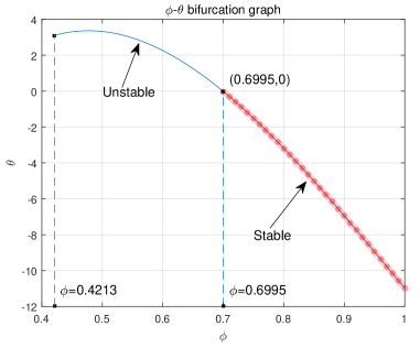
Figure 3: $\varphi$-$\vartheta$ bifurcation graph, $\varphi\in[\frac{4.44}{10.54},1]$

According to above analyses, we take different values of $\varphi$ to observe the dynamics of system (4.1) via numerical simulation. Firstly, taking $\varphi=0.73$, one can see that the orbit emanating from initial value $x^{0}=(0.5,0.6,0.4)$ for the Poincar$\acute{\rm e}$ map $\tilde{S}$ generated by system (4.1) tends to the heteroclinic cycle $\tilde{\Gamma}$ from Figure 4. The corresponding solution flow is indicated in Figure 5, which states that system (4.1) possesses the May-Leonard phenomenon.

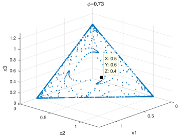
Figure 4: Tend to $\tilde{\Gamma}$

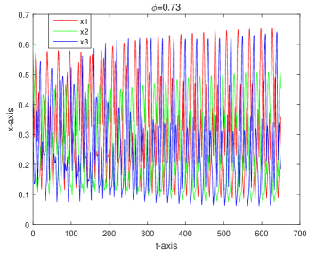
Figure 5: Tend to $\tilde{\Gamma}$

When taking $\varphi=0.631$ and $\varphi=0.629$, one can see that the orbit emanating from initial value $x^{0}=(0.5,0.6,0.4)$ for $\tilde{S}$ tends to invariant closed curves from Figure 6 and Figure 7. Meanwhile, we also find that the invariant closed curve shrinks as $\varphi$ decreases.

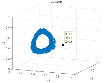
Figure 6: Tend to invariant closed curve

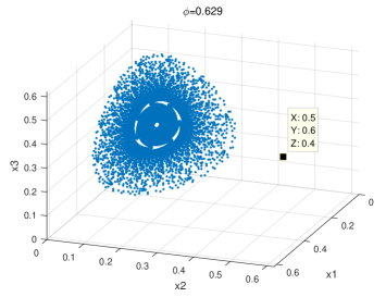
Figure 7: Tend to invariant closed curve

When taking $\varphi=0.61$ $\varphi=0.59,\varphi=0.58$ and $\varphi=0.52$, one can see that the invariant closed curve for $\tilde{S}$ has degenerated into a positive fixed point from Figure 8-12. Furthermore, The patterns converging to positive fixed points are rich and varied.

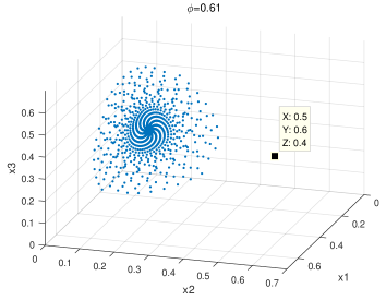
Figure 8: Tend to the positive fixed point

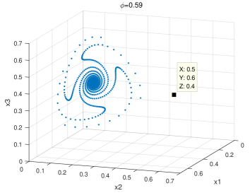
Figure 9: Tend to the positive fixed point

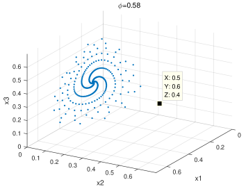
Figure 10: Tend to the positive fixed point

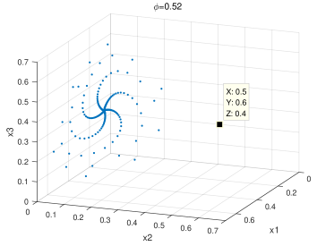
Figure 11: Tend to the positive fixed point

By Theorem 4.1, when $\varphi\in[0,$ $\frac{4.44}{10.54})$, system (4.1) does not admit the heteroclinic cycle. Using numerical simulation, we find that the orbit emanating from initial value $x^{0}=(0.5,0.6,0.4)$ for $\tilde{S}$ tends to different fixed points as $\varphi$ decreases gradually. More precisely, when taking $\varphi=0.39$, one can see that the orbit for $\tilde{S}$ tends to a positive fixed point from Figure 13; when taking $\varphi=0.36$, one can see that the orbit for $\tilde{S}$ tends to the interior fixed point of coordinate plane $\{x_{2}=0\}$ from Figure 14; when taking $\varphi=0.34$, one can see that the orbit for $\tilde{S}$ tends to the interior fixed point of $x_{1}$-axis from Figure 15; when taking $\varphi=0.22$, one can see that the orbit for $\tilde{S}$ tends to the interior fixed point of coordinate plane $\{x_{3}=0\}$ from Figure 16; when taking $\varphi=0.1$, one can see that the orbit for map $\tilde{S}$ tends to the interior fixed point of $x_{2}$-axis from Figure 17; when taking $\varphi=0.09$, one can see that the orbit for $\tilde{S}$ tends to the trivial fixed point $O$ from Figure 18.

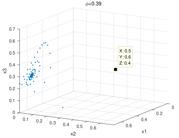
Figure 12: Tend to the positive fixed point

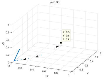
Figure 13: Tend to the interior fixed point of $\{x_{2}=0\}$

In conclusion, compared to the classical May-Leonard competition model (1.1), system (4.1) has much richer dynamics as $\varphi$ varies. To be more explicit, when $\varphi$ varies in $[0,1]$, system (4.1) enjoys different dynamic features: the orbit emanating from initial value $x^{0}=(0.5,0.6,0.4)$ for the Poincar$\acute{\rm e}$ map $\tilde{S}$ tends to the heteroclinic cycle $\tilde{\Gamma}$(see Figure 4) $\rightarrow$ invariant closed curves (see Figure 6 and Figure 7) $\rightarrow$ positive fixed points (see Figure 8-12) $\rightarrow$ the interior fixed point of coordinate plane $\{x_{2}=0\}$ (see Figure 13) $\rightarrow$ the interior fixed point of $x_{1}$-axis (see Figure 14) $\rightarrow$ the interior fixed point of the coordinate plane $\{x_{3}=0\}$ (see Figure 15) $\rightarrow$ the interior fixed point of $x_{2}$-axis (see Figure 16) $\rightarrow$ the trivial fixed point $O$ (see Figure 17).

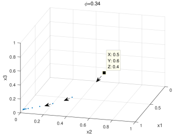
Figure 14: Tend to the interior fixed point of $x_{1}$-axis

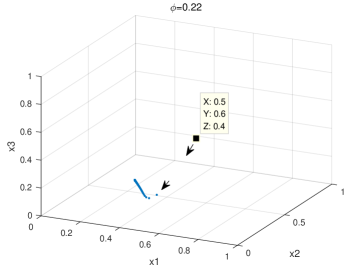
Figure 15: Tend to the interior fixed point of $\{x_{3}=0\}$

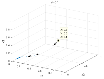
Figure 16: Tend to the interior fixed point of $x_{2}$-axis

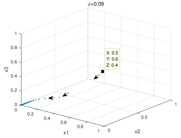
Figure 17: Tend to the trivial fixed point $O$

5 Discussion

In this paper, we focus on a symmetric May-Leonard competition model with seasonal succession. By virtue of the carrying simplex, we obtain that system (1.2) admits a heteroclinic cycle connecting three axial fixed point $R_{i},i=1,2,3$, which is the boundary of the carrying simplex. By the stability theory of heteroclinic cycles for discrete kolmogorov competitive maps proposed by Jiang et al. [15], the stability criterion of the heteroclinic cycle for system (1.2) is established. Especially, when $\lambda_{1}=\lambda_{2}=\lambda_{3}$ and $\alpha+\beta\neq 2$, it is shown that system (1.2) inherits stability properties of the heteroclinic cycle of the classical May-Leonard competition model (1.1), which implies that the stability of the heteroclinic cycle has not been changed by the introduction of seasonal succession in this case. Besides, we also present the explicit expression of the carrying simplex, which states that the carrying simplex is flat in the special case. Applying the stability criterion to a given system (4.1), we obtain that the stability bifurcation of the heteroclinic cycle for such a system. By numerical simulation, we not only illustrate the effectiveness of our theoretical results, but also exhibit rich dynamics (including nontrivial periodic solutions, invariant closed curves and heteroclinic cycles) for the system. Compared to concrete discrete-time competitive maps discussed in [6, 7, 13, 14, 16], the dynamic patterns converging to invariant closed curves and positive fixed points for system (4.1) are much richer. We guess that the interesting and beautiful dynamic patterns are generated by the switching between two subsystems.

In addition, lots of numerical simulations strongly suggest that if system (1.2) has one positive periodic solution, then the positive periodic solution is unique. The estimate for the Floquet multipliers of the positive periodic solution and the complete classification for the global dynamics of system (1.2) are all challenging problems for us. We will leave them for future research.

References

- [1] P. G. Barrientos, J. . Rodriguez and A. Ruiz-Herrera, Chaotic dynamics in the seasonally forced SIR epidemic model, J. Math. Biol., 75(2017), 1655-1668.
- [2] C. W. Chi, S. B. Hsu and L. I. Wu, On the asymmetric May-Leonard model of three competing species. SIAM J. Appl. Math., 58(1)(1998), 211-226.
- [3] J. M. Cushing, Two species competition in a periodic environment, J. Math. Biol., 10(1980), 385–400.
- [4] O. Diekmann, Y. Wang and P. Yan, Carrying simplices in discrete competitive systems and age-structured semelparous populations. Discrete Contin. Dyn. Syst., 20(2008), 37-52.
- [5] M. Field and J. W. Swift, Stationary bifurcation to limit cycles and heteroclinic cycles, Nonlinearity, 4(1991), 1001-1043.
- [6] M. Gyllenberg, J. Jiang, L. Niu and P. Yan, On the classification of generalized competitive Atkinson-Allen models via the dynamics on the boundary of the carrying simplex. Discrete Contin. Dyn. Syst., 38(2018), 615-650.
- [7] M. Gyllenberg, J. Jiang, L. Niu and P. Yan, Permanence and universal classification of discrete-time competitive systems via the carrying simplex. Discrete Contin. Dyn. Syst., 40(2020), 1621-1663.
- [8] S. S. Hu and A. J. Tessier, Seasonal succession and the strength of intra- and interspecific competition in a Daphnia assemblage, Ecology, 76(1995), 2278–2294.
- [9] M. Han, X. Hou, L. Sheng and C. Wang, Theory of rotated equations and applications to a population model, Discrete Contin. Dyn. Syst., 38(4)(2018), 2171-2185.
- [10] S. B. Hsu and X. Q. Zhao, A Lotka-Volterra competition model with seasonal succession, J. Math. Biol., 64(2012), 109-130.
- [11] Z. Y. Hou and S. Baigent, Heteroclinic limit cycles in competititve Kolmogorov systems. Discrete Contin. Dyn. Syst., 33(2013), 4071-4093.
- [12] J. Jiang, L. Niu and D. Zhu, On the complete classification of nullcline stable competitive three-dimensional Gompertz models. Nonlinear Analysis: Real World Applications, 20(2014), 21-35.
- [13] J. Jiang and L. Niu, On the equivalent classification of three-dimensional competitive Atkinson/Allen models relative to the boundary fixed points. Discrete Contin. Dyn. Syst., 36(2016), 217-244.
- [14] J. Jiang and L. Niu, On the equivalent classification of three-dimensional competitive Leslie/Gower models via the boundary dynamics on the carrying simplex. J. Math. Biol., 74(2017), 1223-1261.
- [15] J. Jiang, L. Niu and Y. Wang, On heteroclinic cycles of competitive maps via carrying simplices. J. Math. Biol., 72(2016), 939-972.
- [16] J. Jiang and L. Niu, On the validity of Zeeman’s classification for three dimensional competitive differential equations with linearly determined nullclines. J. Differential Equations, 263(2017), 7753-7781.
- [17] A. L. Koch, Coexistence resulting from an alternation of density dependent and density independent growth. J. Theor. Biol., 44(1974), 373–386.
- [18] C. A. Klausmeier, Successional state dynamics: A novel approach to modeling nonequilibrium foodweb dynamics, J. Theor. Biol., 262(2010), 584-595.
- [19] M. Krupa and I. Melbourne, Asymptotic stability of heteroclinic cycles in systems with symmetry. Ergod. Th. Dynam. Sys., 15(1995), 121-147.
- [20] M. Krupa and I. Melbourne, Asymptotic stability of heteroclinic cycles in systems with symmetry. II, Proc. of Royal Soc. of Edinburgh, 134A(2004), 1177-1197.
- [21] D. L. DeAngelis, J. C. Trexler and D. D. Donalson, Competition dynamics in a seasonally varyingwetland. In: Cantrell S, Cosener C, Ruan S (eds) Spatial ecology, chap 1. CRC Press/Chapman and Hall, London pp 1–13, 2009.
- [22] E. Litchman and C. A. Klausmeier, Competition of phytoplankton under fluctuating light, Am. Naturalist, 157(2001), 170-187.
- [23] J. D. Murray, Mathematical Biology I: An Introduction. 3rd ed, Springer-Verlag, Berlin, 2002.
- [24] R. M. May and A. R. McLean, Theoretical Ecology: Principles and Applications. 3rd ed, Oxford, UK, 2007.
- [25] R. M. May and W. J. Leonard, Nonlinear aspects of competition between three species. SIAM J. Appl. Math., 29(2)(1975), 243-253.
- [26] L. Niu, Y. Wang and X. Xie, Carrying simplex in the Lotka-Volterra competition model with seasonal succession with applications, Discrete Cont. Dyn-B, 26(4)(2021), 2161-2172.
- [27] L-I. W. Roeger and L. J. S. Allen, Discrete May-Leonard competition models I. J. Diff. Equ. Appl., 10(1)(2004), 77-98.
- [28] C. F. Steiner, A. S. Schwaderer, V. Huber, C. A. Klausmeier, E. Litchman,2009. Periodically forced food chain dynamics: model predictions and experimental validation, Ecology, 90(2009), 3099–3107.
- [29] H. L. Smith, Monotone Dynamical Systems. An Introduction to the Theory of Competitive and Cooperative Systems, Math. Surveys Monogr. 41, AMS, Providence, RI, 1995.
- [30] P. Schuster, K. Sigmund and R.Wolff, On limits for competition between three species. SIAM J. Appl. Math., 37(1)(1979), 49-54.
- [31] U. Sommer, Z. M. Gliwicz, W. Lampert and A. Duncan, The PEG-model of seasonal succession of planktonic events in fresh waters, Archiv fr Hydrobiologie, 106(1986), 433-471.
- [32] Y. L. Tang, D. M. Xiao, W. N. Zhang and D. Zhu, Dynamics of epidemic models with asymptomatic infection and seasonal succession, Math. Biosci. Eng., 14(2017), 1407-1424.
- [33] Y. Wang and J. Jiang, Uniqueness and attractivity of the carrying simplex for discrete-time competitive dynamical systems, J. Differential Equations, 186(2002), 611-632.
- [34] D. Xiao, Dynamics and bifurcation on a class of population model with seasonal constant-yield harvesting, Discrete Contin. Dyn. Syst., 21(2016), 699-719.
- [35] Y. X. Zhang and X. Q. Zhao, Bistable travelling waves for reaction and diffusion model with seasonal succession, Nonlinearity, 26(2013), 691-709.