An adaptive model hierarchy for data-augmented training of kernel models for reactive flow

1 Reference model

We are interested in constructing efficient and accurate models to approximate time-dependent quantities of interest (QoI) $f\in L^{2}\big{(}\mathcal{P};L^{2}([0,T])\big{)}$ in the context of reactive flow, with $T>0$ and where $\mathcal{P}\subset\mathbb{R}^{p}$ for $p\geq 1$ denotes the set of possible input parameters. As a class of QoI functions, we consider those obtained by applying linear functionals $s_{\mu}\in V^{\prime}$ to solution trajectories $c_{\mu}\in L^{2}(0,T;V)$ of, e.g., parametric parabolic partial differential equations. Thus, $f(\mu;t):=s_{\mu}(c_{\mu}(t))$, where for each parameter $\mu\in\mathcal{P}$, the concentration $c_{\mu}$ with $\partial_{t}c_{\mu}\in L^{2}(0,T;V^{\prime})$ and initial condition $c_{0}\in V$ is the unique weak solution of

$$\left<\partial_{t}c_{\mu},v\right>+a_{\mu}(c_{\mu},v)=l_{\mu}(v) \forall\;v\in V,\;c_{\mu}(0)=c_{0}.$$ (1)

Here, $V\subset H^{1}(\Omega)\subset L^{2}(\Omega)\subset V^{\prime}$ denotes a Gelfand triple of Hilbert-spaces associated with a spatial Lipschitz-domain $\Omega$ and, for $\mu\in\mathcal{P}$, $l_{\mu}\in V^{\prime}$ denotes a continuous linear functional and $a_{\mu}:V\times V\to\mathbb{R}$ a continuous coercive bilinear form.

As a basic model for reactive flow in catalytic filters, (1) could stem from a single-phase one-dimensional linear advection-diffusion-reaction problem with Dammköhler- and Péclet-numbers as input (thus $p=2$), where $c$ models the dimensionless molar concentration of a species and the break-through curve $s$ measures the concentration at the outflow, as detailed in Gavrilenko et al. (2022).

Since direct evaluations of $f$ are not available, we resort to a full order model (FOM) as reference model, yielding

$$f_{h}:\mathcal{P}\to\mathbb{R}^{N_{T}}\text{ for }N_{T}\geq 1, f_{h}(\mu;t):=s_{\mu}(c_{h,\mu}(t)),$$ (2)

which we assume to be a sufficiently accurate approximation of the QoI. For simplicity, we consider a $P^{1}$-conforming Finite Element space $V_{h}\subset V$ and obtain the FOM solution trajectory $c_{h,\mu}\in L^{2}(0,T;V_{h})$ by Galerkin projection of (1) onto $V_{h}$ and an implicit Euler approximation of the temporal derivative.

2 Surrogate models

The evaluation of (2) may be arbitrarily costly, in particular in multi- or large-scale scenarios where $\dim V_{h}\gg 1$, but also if $N_{T}\gg 1$ due to long-time integration or when a high resolution of $f_{h}$ is required. We thus seek to build a machine learning (ML) based surrogate model

$$f_{\text{ml}}:\mathcal{P}\to\mathbb{R}^{N_{T}},\;f_{\text{ml}}(\mu;t_{n})\approx f_{h}(\mu;t_{n})\;\forall 1\leq n\leq N_{T},$$ (3)

to predict all values $\{f_{\text{ml}}(\mu;t_{n})\}_{n=1}^{N_{T}}$ at once, without time-integration. Such models based on Neural Networks or Kernels typically rely on a large amount of training data

$$\big{\{}\big{(}\mu,f_{h}(\mu)\big{)}\,\big{|}\,\mu\in\mathcal{P}_{\text{train}}\big{\}}, \mathcal{P}_{\text{train}}\subset\mathcal{P}, |\mathcal{P}_{\text{train}}|\gg 1,$$ (4)

rendering their training prohibitively expensive in the aforementioned scenarios; we refer to Gavrilenko et al. (2022) and the references therein and in particular to Santin and Haasdonk (2021). In Gavrilenko et al. (2022) we thus seek to employ an intermediate surrogate to generate sufficient training data.

2.1 Structure preserving Reduced Basis models

The idea of projection-based model order reduction by Reduced Basis (RB) methods is to approximate the state $c_{h}$ in a low-dimensional subspace $V_{\text{rb}}\subset V_{h}$ and to obtain online-efficient approximations of $f_{h}$ by Galerkin projection of the FOM detailed in Section 1 onto $V_{\text{rb}}$ and a pre-computation of all quantities involving $V_{h}$ in a possibly expensive offline-computation; we refer to Milk et al. (2016) and the references therein. Using such structure preserving reduced order models (ROM)s we obtain RB trajectories $c_{\text{rb},\mu}\in L^{2}(0,T;V_{\text{rb}})$ and a RB model

$$f_{\text{rb}}:\mathcal{P}\to\mathbb{R}^{N_{T}}, f_{\text{rb}}(\mu;t):=s_{\mu}(c_{\text{rb},\mu}(t)),$$ (5)

with a computational complexity independent of $\dim V_{h}$, the solution of which, however, still requires time-integration.

The quality and efficiency of RB models hinges on the problem adapted RB space $V_{\text{rb}}$ which could be constructed in an iterative manner steered by a posteriori error estimates using the POD-greedy algorithm from Haasdonk (2013). Instead, we obtain by the method of snapshots

$$V_{\text{rb}}:=\left<\texttt{POD(}\{c_{h,\mu}\,|\,\mu\in\mathcal{P}_{\text{rb}}\texttt{)}\right>, \text{with }\mathcal{P}_{\text{rb}}\subset\mathcal{P}$$ (6)

consisting of only few a priori selected parameters (e.g. the outermost four points in $\mathcal{P}$), where we use the hierarchic approximate POD from Himpe et al. (2018) for $N_{T}\gg 1$ to avoid computing the SVD of a dense snapshot Gramian of size $N_{T}^{2}$.

2.2 Kernel models

While still requiring time-integration, we can afford to use RB ROMs to generate a sufficient amount of training data

$$X_{\text{train}}=\big{\{}\big{(}\mu,f_{\text{rb}}(\mu)\big{)}\,\big{|}\,\mu\in\mathcal{P}_{\text{ml}}\big{\}}\cup\big{\{}\big{(}\mu,f_{h}(\mu)\,\big{|}\,\mu\in\mathcal{P}_{\text{rb}}\big{)}\big{\}},$$

augmented by the FOM-data available as a side-effect from generating $V_{\text{rb}}$. Using this data, we obtain the ML model $f_{\text{ml}}$ from (3) using the vectorial greedy orthogonal kernel algorithm from Santin and Haasdonk (2021).

While resulting in substantial computational gains, the presented approach from Gavrilenko et al. (2022) still relies on the traditional offline/online splitting of the computational process to train the RB ROM as well as the ML model to be valid for all of $\mathcal{P}$, requiring a priori choices regarding $\mathcal{P}_{\text{rb}}$ and $\mathcal{P}_{\text{ml}}$ with a significant impact on the overall performance and applicability of these models.

3 An adaptive model hierarchy

Keil et al. (2021) introduced an approach beyond the classical offline/online splitting where a RB ROM is adaptively enriched based on rigorous a posteriori error estimates, following the path of an optimization procedure through the parameter space. Similarly, we propose an adaptive enrichment yielding a hierarchy of FOM, RB ROM and ML models, based on the standard residual-based a posteriori estimate on the RB output error, $\|f_{h}(\mu)-f_{\text{rb}}(\mu)\|_{L^{2}([0,T]))}\leq\Delta_{\text{rb}}(\mu)$, for which we refer to the references in Milk et al. (2016).

Algorithm 1 Adaptive QoI model generation

1:ROM tolerance $\varepsilon>0$, ML trust/train criteria

2:$X_{\text{train}}=\emptyset$, $\Phi_{\text{RB}}=\{\}$, $V_{\text{rb}}:=\left<\Phi_{\text{rb}}\right>$, $f_{\text{ml}}:=0$

3:for all $\mu\in\mathcal{P}$ selected by outer loop do

4:     if ML model is trustworthy then return $f_{\text{ml}}(\mu)$

5:     else

6:         compute $f_{\text{rb}}(\mu)$, $\Delta_{\text{rb}}(\mu)$

7:         if $\Delta_{\text{rb}}(\mu)\leq\varepsilon$ then

8:              collect $X_{\text{train}}=X_{\text{train}}\cup\{(\mu,f_{\text{rb}}(\mu))\}$

9:              (optionally) fit ML model, return $f_{\text{rb}}(\mu)$

10:         else$\Pi_{\Phi_{\text{rb}}}$: orth. proj. onto $\left<\Phi_{\text{rb}}\right>$

11:              compute $f_{h}(\mu)$

12:              enrich $\Phi_{\text{rb}}=\Phi_{\text{rb}}\cup\texttt{POD(}c_{h}(\mu)-\Pi_{\Phi_{\text{rb}}}[c_{h}(\mu)]\texttt{)}$

13:              update RB ROM

14:              collect $X_{\text{train}}=X_{\text{train}}\cup\{(\mu,f_{h}(\mu))\}$

15:              (optionally) fit ML model, return $f_{h}(\mu)$               

As a means to judge if a ML model is trustworthy, we propose a manual validation using the following a posteriori error estimate on the ML QoI error. While not as cheaply computable as $f_{\text{ml}}$, it still allows to validate the ML model without computing $f_{h}$.

Proposition 1 (ML model a posteriori error estimate)

Let $f_{\text{rb}}(\mu)$, $f_{\text{ml}}(\mu)\in\mathbb{R}^{N_{T}}$ denote the RB ROM and ML model approximations of $f_{h}(\mu)$, respectively, and let $\Delta_{\text{rb}}(\mu)$ denote an upper bound on the RB-output error. We then have by triangle inequality for all $\mu\in\mathcal{P}$

$$\|f_{h}(\mu)-f_{\text{ml}}(\mu) \|_{L^{2}([0,T])}\leq\Delta_{\text{rb}}(\mu)$$ (7)

$$+\|f_{\text{rb}}(\mu)-f_{\text{ml}}(\mu)\|_{L^{2}([0,T])},$$

where the right hand side is computable with a computational complexity independent of $\dim V_{h}$.

Applying Algorithm 1 to the example of one-dimensional single-phase reactive flow from the last row of Table 1 in Gavrilenko et al. (2022), with $\dim\mathcal{P}=2$, $N_{T}=24576$ time steps, $\dim V_{h}=65537$ gives the behaviour shown in Figure 1, where we set $\varepsilon=10^{-2}$, retrain the ML model every 10 collected samples and unconditionally trust the ML model as soon as $|X_{\text{train}}|\geq 50$. For the considered diffusion dominated regime, we only require a single evaluation of $f_{h}$ (yielding a $\dim V_{\text{rb}}=15$-dimensional RB ROM), which results in even further computational savings, compared to the results obtained in Gavrilenko et al. (2022).

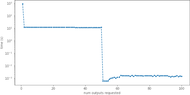
Figure 1: Each dot correspond to the input-to-output query time of the adaptive model from Algorithm 1 applied to Gavrilenko et al. (2022).

References

- Gavrilenko et al. (2022) Gavrilenko, P., Haasdonk, B., Iliev, O., Ohlberger, M., Schindler, F., Toktaliev, P., Wenzel, T., and Youssef, M. (2022). A full order, reduced order and machine learning model pipeline for efficient prediction of reactive flows. In Large-Scale Scientific Computing, 378–386. Springer International Publishing.
- Haasdonk (2013) Haasdonk, B. (2013). Convergence rates of the POD-greedy method. ESAIM Math. Model. Numer. Anal., 47(3), 859–873.
- Himpe et al. (2018) Himpe, C., Leibner, T., and Rave, S. (2018). Hierarchical Approximate Proper Orthogonal Decomposition. SIAM Journal on Scientific Computing, 40(5), A3267–A3292.
- Keil et al. (2021) Keil, T., Mechelli, L., Ohlberger, M., Schindler, F., and Volkwein, S. (2021). A non-conforming dual approach for adaptive trust-region reduced basis approximation of PDE-constrained parameter optimization. ESAIM Math. Model. Numer. Anal., 55(3), 1239–1269.
- Milk et al. (2016) Milk, R., Rave, S., and Schindler, F. (2016). pyMOR – generic algorithms and interfaces for model order reduction. SIAM J. Sci. Comput., 38(5), S194–S216.
- Santin and Haasdonk (2021) Santin, G. and Haasdonk, B. (2021). Kernel methods for surrogate modeling. In P. Benner, S. Grivet-Talocia, A. Quarteroni, G. Rozza, W. Schilders, and L.M. Silveira (eds.), Model Order Reduction, volume 2, 311–353. De Gruyter.