SCHA-VAE: Hierarchical Context Aggregation for Few-Shot Generation
Abstract
A few-shot generative model should be able to generate data from a novel distribution by only observing a limited set of examples. In few-shot learning the model is trained on data from many sets from distributions sharing some underlying properties such as sets of characters from different alphabets or objects from different categories. We extend current latent variable models for sets to a fully hierarchical approach with an attention-based point to set-level aggregation and call our method SCHA-VAE for Set-Context-Hierarchical-Aggregation Variational Autoencoder. We explore likelihood-based model comparison, iterative data sampling, and adaptation-free out-of-distribution generalization. Our results show that the hierarchical formulation better captures the intrinsic variability within the sets in the small data regime. This work generalizes deep latent variable approaches to few-shot learning, taking a step toward large-scale few-shot generation with a formulation that readily works with current state-of-the-art deep generative models.
1 Introduction
Humans are exceptional few-shot learners able to grasp concepts and function of objects never encountered before (Lake et al., 2011). This is because we build internal models of the world so we can combine our prior knowledge about object appearance and function to make well educated inferences from very little data (Tenenbaum, 1999; Lake et al., 2017; Ullman & Tenenbaum, 2020). In contrast, traditional machine learning systems have to be trained tabula rasa and therefore need orders of magnitude more data. In the landmark paper on modern few-shot learning Lake et al. (2015) demonstrated that with a strong prior hand-written symbols from different alphabets can be generated few-shot and distinguished one-shot, i.e. when a letter is shown for the first time.
Few-shot learning (Vinyals et al., 2016; Snell et al., 2017; Finn et al., 2017) and related approaches aiming at learning from little labelled data at test time (Schaul & Schmidhuber, 2010; Hospedales et al., 2020) have recently gained new interest thanks to modeling advances, availability of large diverse datasets and computational resources. Building efficient learning systems that can adapt at inference time is a prerequisite to deploy such systems in realistic settings. Much attention has been devoted to supervised few-shot learning. The problem is typically cast in terms of an adaptive conditional task, where a small support set is used to condition explicitly (Garnelo et al., 2018a) or implicitly (Finn et al., 2017) a learner, with the goal to perform well on a query set. The high-level idea is to train the model with a large number of small sets, and inject in the model the capacity to adapt to new concepts from few-samples at test time.
Comparatively less work has been developed on few-shot adaptation in generative models (Edwards & Storkey, 2016; Reed et al., 2017; Bartunov & Vetrov, 2018). This is partially because of the challenging nature of learning joint distributions in an unsupervised way from few-samples and difficulties in evaluating such models. Few-shot generation has been limited to simple tasks, shallow and handcrafted conditioning mechanisms and as pretraining for supervised few-shot learning. Consequently there is a lack of quantitative evaluation and progress in the field.
In this work we aim to solve these issues for few-shot generation in latent variable models. This class of models is promising because provides a principle way to include adaptive conditioning using latent variables. The setting we consider is that of learning from a large quantity of homogeneous sets, where each set is an un-ordered collections of samples of one concept or class. At test time, the model will be provided with sets of concepts never encountered during training and sets of different cardinality. We consider explicit conditioning in a hierarchical formulation, where global latent variables carry information about the set at hand. A pooling mechanism aggregates information from the set using a hard-coded (mean, max) or learned (attention) operator. The conditioning mechanism is implemented in a shallow or hierarchical way: the hierarchical approach helps to learn better representations for the input set and gradually merges global and local information between the aggregated set and samples in the set. To handle input sets of any size the mechanism has to be permutation invariant. The conditional hierarchical model can naturally represent a family of generative models, each specified by a different conditioning set-level latent variable. Learning a full distribution over the input set increases the flexibility of the model.
Contribution.
-
•
We increase the input set representation expressivity of latent variable models for sets through hierarchical inference and a learnable aggregation mechanism.
-
•
We explore forward and iterative sampling strategies for the marginal and the predictive distributions implicitly defined by few-shot generative models.
-
•
We study the few-shot transfer for this new class of models, exploring generalization to set cardinality, new classes and new datasets, providing evidence that a hierarchical set representation increases the expressivity of few-shot generative models.
2 Generative Models over Sets
In this section we present the modeling background for the proposed few-shot generative models. The Neural Statistician (NS, (Edwards & Storkey, 2016)) is a latent variable model for few-shot learning. Based on this model, many other approaches have been developed (Garnelo et al., 2018b; Bartunov & Vetrov, 2018; Hewitt et al., 2018). The NS is a hierarchical model where two collections of latent variable are learned: a task-specific summary statistic with prior and a per-sample latent variable with prior :
| (1) |
where assuming the data set size is and in general is a hierarchy of latent variables (Sønderby et al., 2016; Maaløe et al., 2019): with .
In the original NS model, the authors factorize the lower-bound wrt and as:
| (2) |
where and is in general a hierarchy of latent variables. In the NS, the moments of the conditioning distribution over are computed using a simple sum/average based formulation ; and then is used to condition . This idea is simple and straightforward, is permutation invariant, enabling efficient learning and a clean lower-bound factorization. But it has a limitation: with such formulation the model expressivity and capacity to extract information from the set are limited. The pooling mechanism assumes strong homogeneity in the context set and the generative process. However, the model formulation opens the door for more advanced invariant aggregations based on attention (Vaswani et al., 2017) and graph approaches (Velickovic et al., 2017)).
In the next section, we move beyond simple aggregation to learn more expressive few-shot generative models able to deal with variety and complexity in the conditioning set. We propose a hierarchical merging of information between conditioning and sample ; and a learnable agggregation mechanism for the context set.
3 Hierarchical Few-Shot Generative Models
Our goal is to learn a generative model over sets, i.e. unordered collections of observations, able to generalize to new datasets given few samples. In this model, is a collection of latent variables that represent a set . We learn a posterior over conditioned on , able to generate samples accordingly to elements in the input set. The model has to be expressive: I) hierarchical - to increase the functions that the model can represent and improve the joint merging of set-level information and sample information , and II) flexible - to handle input sets of any size and complexity, improving the way the model extracts and organizes information in the conditioning set. A fundamental difference between our proposal and previous models is the intrinsically hierarchical inference procedure over and .
Generative Model.
The generative model factorizes the joint distribution . In particular can be written as:
| (3) |
where are latent for layer in the model and sample in the input set ; is a latent for layer in the model and the input set . We factorize the likelihood and prior terms over the set as:
| (4) | ||||
| (5) |
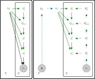
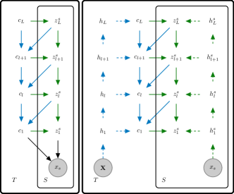
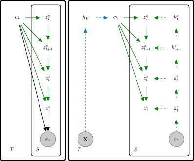
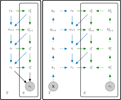
In this formulation the context is a distribution of the previous context representation and the previous latent representation for the samples as illustrated in Figure 3.
Approximate Inference.
Learning in the model is achieved by amortized variational inference (Jordan et al., 1999; Hoffman et al., 2013). The hierarchical formulation leverages structured mean-field approximation to increase inference flexibility. The approximate posterior parameterizes a joint distribution between latent representation for context and samples. We factorize following the generative model:
| (6) |
where we factorize the posterior using a top-down inference formulation (Sønderby et al., 2016), merging top-down stochastic inference with bottom-up deterministic inference from the data. We factorize the posterior terms over the set as:
| (7) | ||||
Lower bound.
In latent variable models (Rezende et al., 2014; Kingma & Welling, 2013) we maximize a per-sample lowerbound over a large dataset. In few-shot generative models we maximize a lower-bound over a large collection of small sets. This detail is important because, even if the dataset of sets is iid by construction, learning in the few-shot scenario relies explicitly on common structure within a small set. For example, each small set can be an unordered collection of observations for a specific class or concept, like a character or face; and we rely on common structure between these observations using aggregation and conditioning on . The variational lower bound for is obtained using the variational distribution :
| (8) | ||||
The lower-bound can be split in three main components: an expected log likelihood term, divergences over and over . The final per-sample loss for sets of size then is , where is the negated lower-bound for set and .
Hierarchical Set Representation.
The core idea in Eq. 8 is that a hierarchical representation for the input set improves few-shot generation. Indeed adding a hierarchy over we largely increase the model capacities. I) The hierarchical formulation for and increases the variational posterior flexibility, and hierarchical inference has been effective to scale per-sample latent variable models to large domains (Maaløe et al., 2019; Vahdat & Kautz, 2020; Child, 2020). Following this reasoning, a hierarchical representation for should increase the model expressivity when dealing with sets. II) We can aggregate context set information at multiple scales and resolution by design, merging a generic with information extracted from previous resolutions. Doing so the model can iteratively refine the class information contained in the set, an essential capacity when dealing with few-samples from a new class. III) The hierarchical formulation gives us also a principle way to share per sample information and per-set information at different level of abstraction in the model, again increasing the model expressivity. IV) On a practical level, the hierarchical formulation can easily be coupled with modern large deep latent variable models (Child, 2020), without the risk of forgetting context information increasing depth or coarse granularity in the context, providing a promising direction for large scale few-shot generative architectures.
3.1 Sampling
We may be interested in either sampling unconditionally or from the predictive distribution . Unconditional sampling may be performed exactly using the generative model as illustrated in Figure 3: first sample the hierarchical prior and then sample the likelihood . Conditional sampling can be done approximately using the variational posterior as a replacement for the exact posterior as outlined in Algorithm 1. In the single pass approach (adapted from the NS) a sample from:
| (9) |
is generated. This approach is not ideal because is only modeled jointly with the latent for the new sample while omitting the latent for . We can introduce this dependence in a Markov chain approach adapted from the missing data imputation framework proposed in Appendix F of (Rezende et al., 2014). We augment with the sample generated in the single pass approach: . From this we can construct a distribution , where is the corresponding augmented latent. From this distribution and the likelihood we can construct a transition kernel:
If then we can show that is an eigen-distribution for the transition kernel and thus sampling the transition kernel will under mild conditions converge to a sample from . There are several ways to construct from the hierarchical variational and prior distributions. One possibility is shown in Algorithm 1. Alternatively, one may sample , generate the remainder of the latent from the prior hierarchy and new samples from the likelihood. If the variational is exact, these approaches are equivalent and exact. In the experimental section we report results for the different approaches.
3.2 Learnable aggregation (LAG)
A central idea in few-shot generative models is to condition the generative model with a permutation invariant representation of the input set. For a NS such operator is a hard-coded per-set statistic. This approach (Edwards & Storkey, 2016; Garnelo et al., 2018b) maps each sample in independently using and then aggregating to generate the moments for . This idea is simple and effective when using homogeneous and small sets for conditioning. Another choice is a relation network (Sung et al., 2018; Rusu et al., 2018) followed by aggregation.
However, the adaptation capacities of the model are a function of how we represent the input set and a more expressive learnable aggregation mechanism can be useful. In the general scenario, a few-shot generative model should be able to extract information from any conditioning set in terms of variety and size. In this paper we consider a multi-head attention-based learnable aggregation (LAG, Algorithm 2) inspired by (Lee et al., 2019) that can be used in each block of the hierarchy over (Figure 4). Using LAG we can account for statistical dependencies in the set, handle variety between samples in the set and generalize better to input set dimensions. In the experimental section we provide extensive empirical analysis of how using LAG improves the generative and transfer capacity of the model. More details in Appendix A.
4 Experiments
In this section we discuss experimental setup and results for our model. In particular for all the models our interests are: I) Quantitative evaluation of few-shot generation; II) Few-shot conditional and unconditional sampling from the model. III) Transfer of generative capacities to new datasets and input set size. IV) Evidence that the hierarchical context representation is useful for the model.
Datasets.
We train models on binarized Omniglot (Lake et al., 2015), CelebA (Liu et al., 2015) and FS-CIFAR100 (Oreshkin et al., 2018). For Omniglot we consider two scenarios: the train-test split (also known as background-evaluation split) proposed in (Lake et al., 2015): in this scenario all the characters at test time are from new alphabets. And the variant proposed in (Edwards & Storkey, 2016), where all the characters are mixed together and randomly assigned to train and test splits. We perform quantitative evaluation on Omniglot, MNIST (LeCun, 1998), DOUBLE-MNIST (Sun, 2019), TRIPLE-MNIST (Sun, 2019), CelebA and FS-CIFAR100. We resize all the binary datasets to 28x28, CIFAR100 to 32x32, and CelebA to 64x64.
Training Details.
We follow the approach proposed in (Edwards & Storkey, 2016) for training with sets. We create a large collection of small sets, where each set contains all or some of the occurrences for a specific class or concept in a dataset: a character for Omniglot; the face of an identity for CelebA. Both datasets contain thousands of characters/identities with an average number of 20 occurrences per class. For this reason they are a natural choice for few-shot generation. Then we split the sets in train/val/test sets. Using these splits we can dynamically create sets of different dimensions, generating a new collection of training sets at each epoch during training. For training we use the episodic approach proposed in (Vinyals et al., 2016). Each input set is a homogeneous (one concept or class) collection of samples. During training the input set size is always between 2 and 20. The NS architecture is a close approximation of (Edwards & Storkey, 2016). We describe additional details in Appendix C.
Baselines.
We use a VAE - which does not explore set information - and the Neural Statistician (NS) as baselines. We consider two main model variants. Such variants are characterized by different design choices for the conditioning mechanism: standard aggregation mechanism (MEAN pooling) and learnable ones (LAG). We also consider a Convolutional Neural Statistician (CNS) where the latent space is shaped with convolutions at a given resolution. We call our approach Set-Context-Hierarchical-Aggregation Variational Autoencoder (SCHA-VAE, pronounced shave) where an additional hierarchy over is employed.
Model Design.
NS-based models are difficult to scale and performance tends to plateau increasing depth. This can be explained considering that has to be shared through all the network and information can easily be lost in the stochastic sampling process. We overcome these challenges and stabilize SCHA-VAE when increasing depth, we use a shared routing path between and : we learn bias term and for the top layer, and merge all sampling information in these paths: and , where and are samples from layer . We then share information through these path, helping to stabilize and preserve information through the hierarchy. We additionally remove any form of normalization (batch/layer norm) in the hierarchical formulation. This is not directly related to performance, but to challenge the model to perform pure few-shot generation at train and test time, without relying on batch statistics. Our implementation is inspired by (Child, 2020).
4.1 Test log-likelihood
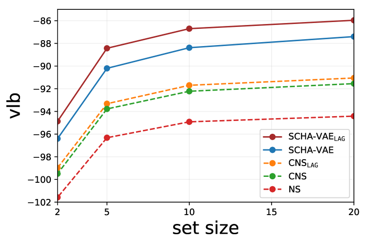
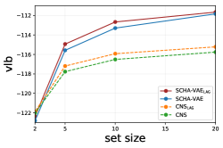
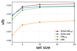
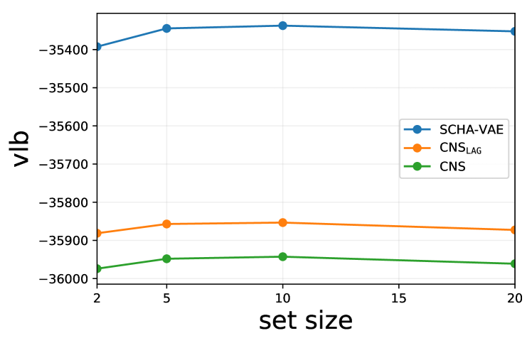
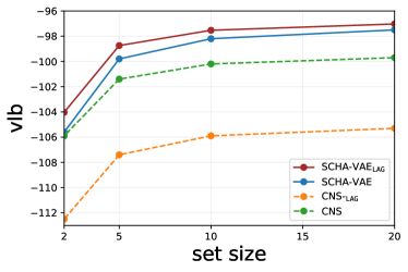
With these experiments we test the generalization properties of the model on few-shot generation. We explore the behavior of the model increasing the input size. Evaluation of generative properties is performed using the log likelihood lower bound (ELBO) and approximating the log marginal likelihood with 1000 importance samples. In Table 1 and 2 we consider few-shot generalization on Omniglot and MNIST with disjoint classes and set size 5. In Figure 1 and 10 we show the models behavior increasing the input set cardinality at test time. All the models are trained with input sets of size 5 on Omniglot. Then at test time we vary the size of the context set between 2 and 20.
| Omniglot-ns | Omniglot-back-eval | MNIST | |||||||
|---|---|---|---|---|---|---|---|---|---|
| Agg | NELBO | NLL (1k) | NELBO | NLL (1k) | NELBO | Params (M) | |||
| VAE | ✓ | 101.5 .1 | 95.9 | 101.4 .1 | 88.4 | 124.7 .1 | |||
| NS | MEAN | ✓ | ✗ | 96.6 .1 | 92.4 | 91.9 .1 | 85.6 | 120.3 .1 | |
| CNS | MEAN | ✓ | ✗ | 92.9 .1 | 89.7 | 83.4 .1 | 77.5 | 118.2 .2 | |
| CNS | LAG | ✓ | ✗ | 92.8 .1 | 89.7 | 83.8 .1 | 77.6 | 117.6 .1 | |
| SCHA-VAE (ours) | MEAN | ✓ | ✓ | 89.4 .1 | 85.8 | 79.4 .1 | 72.7 | 115.3 .2 | |
| SCHA-VAE (ours) | LAG | ✓ | ✓ | 88.4 .3 | 85.4 | 77.9 .3 | 71.5 | 114.9 .1 | |
| Standard | Augmented | |||||||||||||||
|---|---|---|---|---|---|---|---|---|---|---|---|---|---|---|---|---|
| in-distro | out-distro | in-distro | out-distro | |||||||||||||
| 2 | 5 | 10 | 20 | 2 | 5 | 10 | 20 | 2 | 5 | 10 | 20 | 2 | 5 | 10 | 20 | |
| NS | 96.8 | 91.2 | 89.6 | 88.8 | 101.5 | 96.6 | 95.1 | 94.7 | 107.8 | 102.6 | 101.1 | 100.5 | 111.1 | 106.1 | 104.6 | 103.9 |
| CNS | 97.8 | 91.7 | 90.0 | 89.2 | 98.8 | 92.8 | 91.2 | 90.6 | 107.7 | 101.7 | 100.0 | 99.4 | 108.6 | 102.7 | 100.9 | 100.1 |
| SCHA-VAE | 91.5 | 85.2 | 83.5 | 82.7 | 96.2 | 89.7 | 87.9 | 87.0 | 103.0 | 96.6 | 94.8 | 94.1 | 105.9 | 99.2 | 97.2 | 96.2 |
The NS is the original Neural Statistician with mean aggregation. CNS employs a convolutional set representation. The models with LAG use an attention-based learnable aggregation, that builds an adaptive aggregation mechanism for each set. For SCHA-VAE we use the same two aggregation mechanisms. SCHA-VAE improves performance in terms of ELBO and likelihood on different Omniglot test splits and transfer to MNIST without adaptation better than the baselines. The hierarchical formulation for provides most of the improvement. Adding the learnable aggregation mechanism gives an additional boost. Increasing the set (2-20), SCHA-VAE can aggregate more and more information, learning a better model for the data under different regimes (in-distro, out-distro) and augmentation schemes. See Appendix, Table 3 for additional quantitative evaluation with few-shot generative models proposed in the literature, where we compare SCHA-VAE with autoregressive-based models for few-shot generation (Bartunov & Vetrov, 2018; Hewitt et al., 2018).
4.2 Sampling
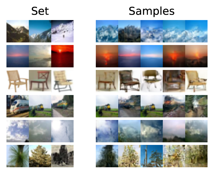
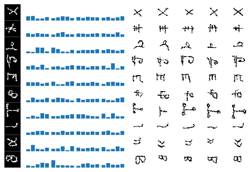
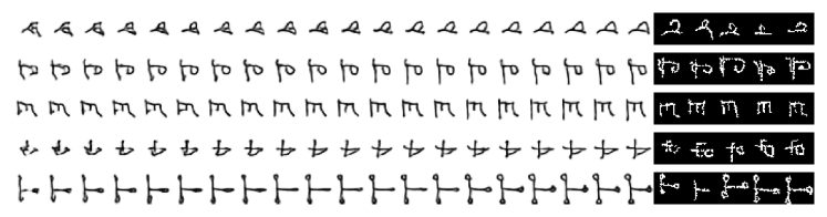
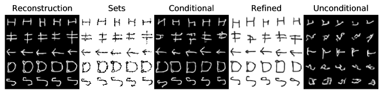
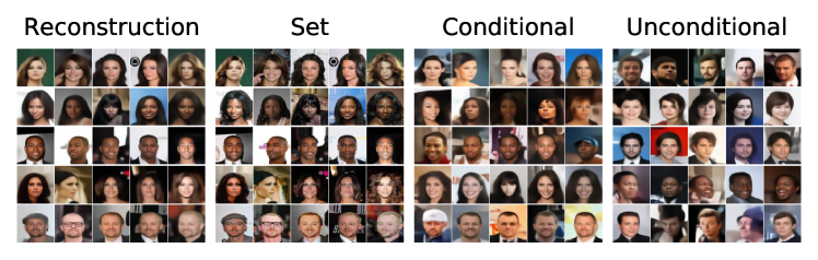
In latent variable models like VAEs we can only perform unconditional sampling. In a NS we have different ways of sampling as explained in Section 3.1. In particular two main sampling approaches can be used: I) conditional sampling, where we sample the predictive distribution relying on the inference model. II) unconditional sampling, sampling through and then . In Figure 11 we show (from left to right) stochastic reconstructions, input sets, conditional samples, and unconditional samples.

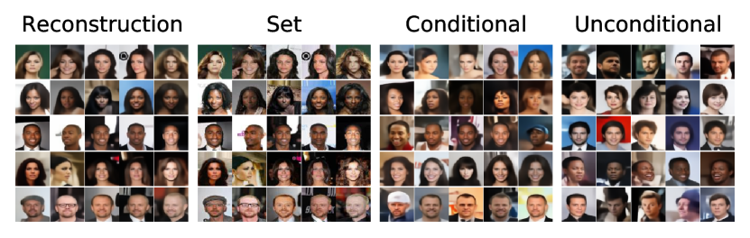
(Bottom): Stochastic reconstruction, input sets, conditional sampling, and unconditional sampling (sometimes referred to as imagination). The models are trained on subsets of CelebA and tested on disjoint identities. Appendix B for larger version.
For simple characters there is almost no difference between conditional and refinement sampling. However, when the model is challenged with a new complex character (Figure 11, top), the refinement procedure greatly improves the adaptation capacities and visual quality of the generated samples. In the rightmost column in the bottom part of Figure 11 we see fully unconditional samples. The model, given a set representation , generates consistent symbols, corroborating the assumption that the model learns a different distribution for each , greatly increasing the model flexibility and representation capacities.
4.3 Transfer
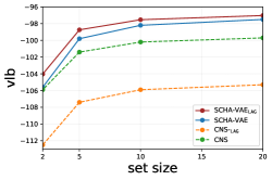
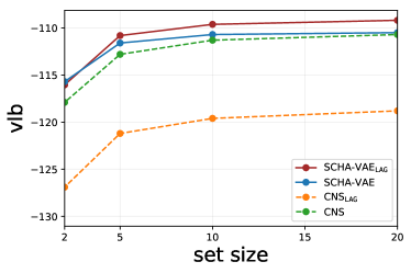
With these experiments we explore few-shot generation in the context of transfer learning. We use the same models we trained on Omniglot and we test on unseen classes in a different dataset. We use MNIST test set (10 classes), DOUBLE-MNIST test set (20 classes) and TRIPLE-MNIST test set (200 classes). The datasets increase in complexity and in size. We expect relatively good performance on the simple one and worse performance on the more complex one. We resize all the datasets to 28x28 pixels using BOX resizing. In Figure 12 we report likelihoods transfer increasing the input set size on the three datasets. Our models perform better on all three datasets. Attention-based aggregation is essential for good performance on few-shot transfer. Again our models perform better than the baselines and attention-based aggregation is important for good performance on concepts from different datasets.
In Appendix B, we report out of distribution classification performance for the three approaches described in Section 3. The models are trained on Omniglot for context size 5 and tested on MNIST also for context size 5 without adapting the distributions to the MNIST data.
4.4 Hierarchy
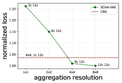
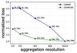
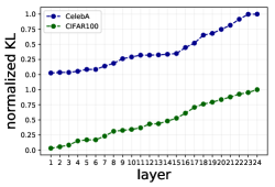
We claim that depth in the set representation and aggregation at multiple resolutions are essential to increase model expressivity. In Fig. 7 we provide empirical evidence. We train SCHA-VAE with 12 stochastic layers on Omniglot, and with 24 layers on CelebA and CIFAR100. At inference, is bypassed for a certain number of layers, without modifying the depth for , effectively decreasing the context depth, and we compute the test ELBO normalizing to one for easier comparison between datasets. If the hierarchy over c is redundant, removing a certain number of layers should not impact the overall result; if instead the model is using aggregation at different resolutions, then the result should be greatly impacted. We see how removing the hierarchical information over worsen greatly the results for all the datasets, providing evidence that the set representation for few-shot generation. On the right we plot the cumulative KL for CelebA and CIFAR100, showing how each layer contains additional information.
5 Related Work
Learning from Sets.
In recent years a large corpus of work studied the problem of learning from sets (Zaheer et al., 2017), and more generally learning in exchangeable deep models (De Finetti, 2020; Bloem-Reddy & Teh, 2020, 2019). These models can be formulated in a variety of ways, but they all have in common a form of permutation invariant aggregation (or pooling mechanism) over the input set. Deep Sets (Zaheer et al., 2017) formalized the framework of exchangeable models. The Neural Statistician (Edwards & Storkey, 2016) was the first model proposing to learn from sets in the variational autoencoder framework and used a simple and effective mean pooling mechanism for aggregation. The authors explored the representation capacities of such model for clustering and few-shot supervised learning. Generative Query Networks performs neural rendering (Eslami et al., 2018) where the problem of pooling views arises. The Neural process family (Garnelo et al., 2018b; Kim et al., 2019), where a set of point is used to learn a context set and solve downstream tasks like image completion and few-shot learning. Set Transformers (Lee et al., 2019) leverages attention to solve problems involving sets. PointNet (Qi et al., 2017) models point clouds as a set of points. Graph Attention Networks (Velickovic et al., 2017) aggregate information from related nodes using attention. Associate Compression Network (Graves et al., 2018) can be interpreted in this framework, where a prior for a VAE is learned using the top-knn retrieved in latent space. In this work we build on ideas and intuitions in these works, with a focus on generative models for sets. SetVAE (Kim et al., 2021) proposes a VAE for point-clouds, showing that processing the input set at multiple resolutions is a promising direction for set-based latent variable models.
Few-Shot Generative Models.
Historically the machine learning community has focused its attention on supervised few-shot learning, solving a classification or regression task on new classes at test time given a small number of labeled examples. The problem can be tackled using metric based approaches (Vinyals et al., 2016; Snell et al., 2017; Oreshkin et al., 2018), gradient-based adaptation (Finn et al., 2017), optimization (Ravi & Larochelle, 2016). More generally, the few-shot learning task can be recast as bayesian inference in hierarchical modelling (Grant et al., 2018; Ravi & Beatson, 2018). In such models, typically parameters or representation are conditioned on the task, and conditional predictors are learned for such task. In (Xu et al., 2019) an iterative attention mechanism is used to learn a query-dependent task representation for supervised few-shot learning. Modern few-shot generation in machine learning was introduced in (Lake et al., 2015). The Neural Statistician (Edwards & Storkey, 2016) is one of the first few-shot learning models in the context of VAEs. However the authors focused on downstream tasks and not on generative modeling. The model has been improved further increasing expressivity for the conditional prior using powerful autoregressive models (Hewitt et al., 2018), a non-parametric formulation for the context (Wu et al., 2020) and exploiting supervision (Garnelo et al., 2018b). (Rezende et al., 2016) proposed a recurrent and attentive sequential generative model for one-shot learning based on (Gregor et al., 2015). Powerful autoregressive decoders and gradient-based adaptation are employed in (Reed et al., 2017) for one-shot generation. The context in this model is a deterministic variable. In GMN (Bartunov & Vetrov, 2018) a variational recurrent model learns a per-sample context-aware latent variable. Similar to our approach, GMN learns a flexible context, learning an attention based kernel that can handle generic datasets. However the context-aware representation scales quadratic with the input size, there is no separation between global and local information in latent space, and the input set is processed in an arbitrary autoregressive order, and not in a permutation invariant manner. Finally, recent large-scale autoregressive language models (Brown et al., 2020) exhibit non-trivial few-shot capacities.
6 Conclusion
Leveraging recent advances in deep latent variable models, we propose a new class of hierarchical latent variable models for few-shot generation. We ground our formulation in hierarchical inference and a learnable non-parametric aggregation. We show how simple hierarchical inference is a viable adaptation strategy. We perform extensive empirical evaluation in terms of generative metrics, sampling capacities and transfer properties. The proposed formulation is completely general and we expect there is large potential for improving performance by combining it with state of the art VAE architectures. Since benchmarks often come with grouping information, using a hierarchical formulation is a generic approach to improve generative capabilities.
Acknowledgement
We would like to thank Anders Christensen, Marco Ciccone, Andrea Dittadi, Pierluca D’Oro, Søren Hauberg, Valentin Liévin, Didrik Nielsen, Mathias Schreiner, Timon Willi, Max Wilson for insightful comments and useful discussions.
References
- Bartunov & Vetrov (2018) Bartunov, S. and Vetrov, D. Few-shot generative modelling with generative matching networks. In International Conference on Artificial Intelligence and Statistics, pp. 670–678, 2018.
- Bloem-Reddy & Teh (2019) Bloem-Reddy, B. and Teh, Y. W. Probabilistic symmetry and invariant neural networks. arXiv preprint arXiv:1901.06082, 2019.
- Bloem-Reddy & Teh (2020) Bloem-Reddy, B. and Teh, Y. W. Probabilistic symmetries and invariant neural networks. Journal of Machine Learning Research, 21(90):1–61, 2020.
- Brown et al. (2020) Brown, T. B., Mann, B., Ryder, N., Subbiah, M., Kaplan, J., Dhariwal, P., Neelakantan, A., Shyam, P., Sastry, G., Askell, A., et al. Language models are few-shot learners. arXiv preprint arXiv:2005.14165, 2020.
- Child (2020) Child, R. Very deep vaes generalize autoregressive models and can outperform them on images. arXiv preprint arXiv:2011.10650, 2020.
- De Finetti (2020) De Finetti, B. 9. on the condition of partial exchangeability. In Studies in Inductive Logic and Probability Volume 2, pp. 193–206. University of California Press, 2020.
- Edwards & Storkey (2016) Edwards, H. and Storkey, A. Towards a neural statistician. arXiv preprint arXiv:1606.02185, 2016.
- Eslami et al. (2018) Eslami, S. A., Rezende, D. J., Besse, F., Viola, F., Morcos, A. S., Garnelo, M., Ruderman, A., Rusu, A. A., Danihelka, I., Gregor, K., et al. Neural scene representation and rendering. Science, 360(6394):1204–1210, 2018.
- Finn et al. (2017) Finn, C., Abbeel, P., and Levine, S. Model-agnostic meta-learning for fast adaptation of deep networks. arXiv preprint arXiv:1703.03400, 2017.
- Garnelo et al. (2018a) Garnelo, M., Rosenbaum, D., Maddison, C. J., Ramalho, T., Saxton, D., Shanahan, M., Teh, Y. W., Rezende, D. J., and Eslami, S. Conditional neural processes. arXiv preprint arXiv:1807.01613, 2018a.
- Garnelo et al. (2018b) Garnelo, M., Schwarz, J., Rosenbaum, D., Viola, F., Rezende, D. J., Eslami, S., and Teh, Y. W. Neural processes. arXiv preprint arXiv:1807.01622, 2018b.
- Grant et al. (2018) Grant, E., Finn, C., Levine, S., Darrell, T., and Griffiths, T. Recasting gradient-based meta-learning as hierarchical bayes. arXiv preprint arXiv:1801.08930, 2018.
- Graves et al. (2018) Graves, A., Menick, J., and van den Oord, A. Associative compression networks for representation learning. CoRR, abs/1804.02476, 2018. URL http://arxiv.org/abs/1804.02476.
- Gregor et al. (2015) Gregor, K., Danihelka, I., Graves, A., Rezende, D. J., and Wierstra, D. Draw: A recurrent neural network for image generation. arXiv preprint arXiv:1502.04623, 2015.
- Hewitt et al. (2018) Hewitt, L. B., Nye, M. I., Gane, A., Jaakkola, T., and Tenenbaum, J. B. The variational homoencoder: Learning to learn high capacity generative models from few examples. arXiv preprint arXiv:1807.08919, 2018.
- Hoffman et al. (2013) Hoffman, M. D., Blei, D. M., Wang, C., and Paisley, J. Stochastic variational inference. The Journal of Machine Learning Research, 14(1):1303–1347, 2013.
- Hospedales et al. (2020) Hospedales, T., Antoniou, A., Micaelli, P., and Storkey, A. Meta-learning in neural networks: A survey. arXiv preprint arXiv:2004.05439, 2020.
- Jordan et al. (1999) Jordan, M. I., Ghahramani, Z., Jaakkola, T. S., and Saul, L. K. An introduction to variational methods for graphical models. Machine learning, 37(2):183–233, 1999.
- Kim et al. (2019) Kim, H., Mnih, A., Schwarz, J., Garnelo, M., Eslami, A., Rosenbaum, D., Vinyals, O., and Teh, Y. W. Attentive neural processes. arXiv preprint arXiv:1901.05761, 2019.
- Kim et al. (2021) Kim, J., Yoo, J., Lee, J., and Hong, S. Setvae: Learning hierarchical composition for generative modeling of set-structured data. In Proceedings of the IEEE/CVF Conference on Computer Vision and Pattern Recognition, pp. 15059–15068, 2021.
- Kingma & Welling (2013) Kingma, D. P. and Welling, M. Auto-encoding variational bayes. arXiv preprint arXiv:1312.6114, 2013.
- Lake et al. (2011) Lake, B., Salakhutdinov, R., Gross, J., and Tenenbaum, J. One shot learning of simple visual concepts. In Proceedings of the annual meeting of the cognitive science society, volume 33, 2011.
- Lake et al. (2015) Lake, B. M., Salakhutdinov, R., and Tenenbaum, J. B. Human-level concept learning through probabilistic program induction. Science, 350(6266):1332–1338, 2015.
- Lake et al. (2017) Lake, B. M., Ullman, T. D., Tenenbaum, J. B., and Gershman, S. J. Building machines that learn and think like people. Behavioral and brain sciences, 40, 2017.
- LeCun (1998) LeCun, Y. The mnist database of handwritten digits. http://yann. lecun. com/exdb/mnist/, 1998.
- Lee et al. (2019) Lee, J., Lee, Y., Kim, J., Kosiorek, A., Choi, S., and Teh, Y. W. Set transformer: A framework for attention-based permutation-invariant neural networks. In International Conference on Machine Learning, pp. 3744–3753. PMLR, 2019.
- Liu et al. (2015) Liu, Z., Luo, P., Wang, X., and Tang, X. Deep learning face attributes in the wild. In Proceedings of International Conference on Computer Vision (ICCV), December 2015.
- Maaløe et al. (2019) Maaløe, L., Fraccaro, M., Liévin, V., and Winther, O. Biva: A very deep hierarchy of latent variables for generative modeling. arXiv preprint arXiv:1902.02102, 2019.
- Oord et al. (2016) Oord, A. v. d., Kalchbrenner, N., and Kavukcuoglu, K. Pixel recurrent neural networks. arXiv preprint arXiv:1601.06759, 2016.
- Oreshkin et al. (2018) Oreshkin, B., Rodríguez López, P., and Lacoste, A. Tadam: Task dependent adaptive metric for improved few-shot learning. Advances in Neural Information Processing Systems, 31:721–731, 2018.
- Perez et al. (2017) Perez, E., Strub, F., De Vries, H., Dumoulin, V., and Courville, A. Film: Visual reasoning with a general conditioning layer. arXiv preprint arXiv:1709.07871, 2017.
- Qi et al. (2017) Qi, C. R., Su, H., Mo, K., and Guibas, L. J. Pointnet: Deep learning on point sets for 3d classification and segmentation. In Proceedings of the IEEE conference on computer vision and pattern recognition, pp. 652–660, 2017.
- Ravi & Beatson (2018) Ravi, S. and Beatson, A. Amortized bayesian meta-learning. In International Conference on Learning Representations, 2018.
- Ravi & Larochelle (2016) Ravi, S. and Larochelle, H. Optimization as a model for few-shot learning. 2016.
- Reed et al. (2017) Reed, S., Chen, Y., Paine, T., Oord, A. v. d., Eslami, S., Rezende, D., Vinyals, O., and de Freitas, N. Few-shot autoregressive density estimation: Towards learning to learn distributions. arXiv preprint arXiv:1710.10304, 2017.
- Rezende et al. (2014) Rezende, D. J., Mohamed, S., and Wierstra, D. Stochastic backpropagation and approximate inference in deep generative models. arXiv preprint arXiv:1401.4082, 2014.
- Rezende et al. (2016) Rezende, D. J., Mohamed, S., Danihelka, I., Gregor, K., and Wierstra, D. One-shot generalization in deep generative models. arXiv preprint arXiv:1603.05106, 2016.
- Rusu et al. (2018) Rusu, A. A., Rao, D., Sygnowski, J., Vinyals, O., Pascanu, R., Osindero, S., and Hadsell, R. Meta-learning with latent embedding optimization. arXiv preprint arXiv:1807.05960, 2018.
- Salimans et al. (2017) Salimans, T., Karpathy, A., Chen, X., and Kingma, D. P. Pixelcnn++: Improving the pixelcnn with discretized logistic mixture likelihood and other modifications. arXiv preprint arXiv:1701.05517, 2017.
- Schaul & Schmidhuber (2010) Schaul, T. and Schmidhuber, J. Metalearning. Scholarpedia, 5(6):4650, 2010.
- Snell et al. (2017) Snell, J., Swersky, K., and Zemel, R. Prototypical networks for few-shot learning. In Advances in Neural Information Processing Systems, pp. 4077–4087, 2017.
- Sønderby et al. (2016) Sønderby, C. K., Raiko, T., Maaløe, L., Sønderby, S. K., and Winther, O. Ladder variational autoencoders. In Advances in neural information processing systems, pp. 3738–3746, 2016.
- Sun (2019) Sun, S.-H. Multi-digit mnist for few-shot learning, 2019. URL https://github.com/shaohua0116/MultiDigitMNIST.
- Sung et al. (2018) Sung, F., Yang, Y., Zhang, L., Xiang, T., Torr, P. H., and Hospedales, T. M. Learning to compare: Relation network for few-shot learning. In Proceedings of the IEEE Conference on Computer Vision and Pattern Recognition, pp. 1199–1208, 2018.
- Tenenbaum (1999) Tenenbaum, J. B. A Bayesian framework for concept learning. PhD thesis, Massachusetts Institute of Technology, 1999.
- Ullman & Tenenbaum (2020) Ullman, T. D. and Tenenbaum, J. B. Bayesian models of conceptual development: Learning as building models of the world. Annual Review of Developmental Psychology, 2:533–558, 2020.
- Vahdat & Kautz (2020) Vahdat, A. and Kautz, J. NVAE: A deep hierarchical variational autoencoder. In Neural Information Processing Systems (NeurIPS), 2020.
- Vaswani et al. (2017) Vaswani, A., Shazeer, N., Parmar, N., Uszkoreit, J., Jones, L., Gomez, A. N., Kaiser, Ł., and Polosukhin, I. Attention is all you need. In Advances in Neural Information Processing Systems, pp. 5998–6008, 2017.
- Velickovic et al. (2017) Velickovic, P., Cucurull, G., Casanova, A., Romero, A., Lio, P., and Bengio, Y. Graph attention networks. arXiv preprint arXiv:1710.10903, 1(2), 2017.
- Vinyals et al. (2016) Vinyals, O., Blundell, C., Lillicrap, T., Wierstra, D., et al. Matching networks for one shot learning. In Advances in neural information processing systems, pp. 3630–3638, 2016.
- Wu et al. (2020) Wu, M., Choi, K., Goodman, N. D., and Ermon, S. Meta-amortized variational inference and learning. In AAAI, pp. 6404–6412, 2020.
- Xu et al. (2019) Xu, J., Ton, J.-F., Kim, H., Kosiorek, A. R., and Teh, Y. W. Metafun: Meta-learning with iterative functional updates. arXiv preprint arXiv:1912.02738, 2019.
- Zaheer et al. (2017) Zaheer, M., Kottur, S., Ravanbakhsh, S., Poczos, B., Salakhutdinov, R. R., and Smola, A. J. Deep sets. In Advances in neural information processing systems, pp. 3391–3401, 2017.
Notation.
Appendix A Model Derivation
In this section we derive the generative model, inference model and lower-bound for a Basic Neural Statistician (bNS), a Neural Statistician (with hierarchy over , this is the model used as baseline in the paper) (NS), and a Hierarchical Few-Shot Generative Model (HFSGM) with hierarchy over and . Doing so we can underline similarities and differences among the formulations.
Set Marginal.
Our goal is to model a distribution where is in general a small set ranging from 1 to 20 samples. We sample these sets from a common process. The Neural Statistician (Edwards & Storkey, 2016) introduces a global latent variable for a set :
| (10) |
Then we can introduce a per-sample latent variable :
| (11) | ||||
where is a set of images, is a latent variable for the set, are latent variable for the samples in the set. The formula above is the basic marginal for all the NS-like model.
A.1 Generative Model
We can think of the model as composed of three components: a hierarchical prior over , a hierarchical prior over , and a render for . For each hierarchical prior, the top distribution is not autoregressive and act as an unconditional prior for and a conditional prior for . In the following all the latent distributions are normal distributions with diagonal covariance. Given the hierarchical nature of our model, these assumptions are not restrictive, because from top to down in the hierarchy we build an expressive structured mean field approximation. The decoder is Bernoulli distributed for binary datasets. In the following equation we use , , , . Each of these equation can be written per-set or per-sample. We choose to write everything in a compact format writing per-set equations.
bNS.
In this setting both and are shallow latent variables:
| (12) |
NS.
is a hierarchy:
| (13) |
HFSGM.
Both and are a hierarchy. We increase the model flexibility.
Using such hierarchy we can:
-
•
learn a structured mean field approximation for ;
-
•
jointly learn and , informing different stages of the learning process;
-
•
incrementally improve through layers of inference.
| (14) | ||||
A.2 Inference Model
We learn the model using Amortized Variational Inference. In a NS-like model, inference is intrinsically hierarchical: the model encodes global set-level information in using .
bNS.
| (15) |
NS.
| (16) |
HFSGM.
| (17) | ||||
A.3 Lower-bound
We learn the model by Amortized Variational Inference similarly to recent methods. However we are in presence of two different latent variables, and we need to lower-bound wrt both.
bNS.
| (18) | ||||
NS.
| (19) | ||||
HFSGM.
| (20) | ||||
A.4 Loss
The final loss for all the models is computed per-sample. Given a distribution of sets (or tasks) of size , the training loss is: .
A.5 Evaluation
For VAEs we evaluate the models approximating the log marginal likelihood using importance samples:
| (21) |
For hierarchical models like the NS we use:
| (22) |
A.6 Learnable Aggregation
In this subsection we describe more explicitly the aggregation mechanism. Given a set , embeddings for samples in the set , and aggregated statistics , we can compute attention weights for a NSLAG as follows:
| (23) | ||||
where , and are linear layers and sim is the dot-product scaled by the square root of the representations dimensionality. This approach is inspired by (Lee et al., 2019) and resembles self-attention with a fundamental difference: instead to map from samples to samples, we map from samples to a per-task learnable aggregation. The query input is a handcrafted aggregation (mean, max pooling). We improve the query scoring the handcrafted aggregation with the samples in the set.
For a full SCHA-VAELAG, we can similarly write:
| (24) | ||||
A.7 Sampling Algorithms
Appendix B Additional Experiments
B.1 Generalization
| CelebA | ||||
|---|---|---|---|---|
| Depth c | Res | Depth | NLL (bpd) | |
| CNS | 1 | 4x4 | 3 | 4.2235 |
| CNSLAG | 1 | 4x4 | 3 | 4.2126 |
| SCHA-VAE | 3 | 4x4 | 3 | 4.1552 |
| Aggregation | Sampling | NLL (nats) | |
|---|---|---|---|
| without autoregressive components | |||
| VHE (Hewitt et al., 2018) | 104.67 | ||
| NS (Edwards & Storkey, 2016) | 102.84 | ||
| CNS | 77.21 | ||
| SCHA-VAE (Ours) | 64.34 | ||
| with autoregressive components | |||
| NS + PixelCNN | 73.50 | ||
| GMN (Bartunov & Vetrov, 2018) | 62.42 | ||
| VHE (Hewitt et al., 2018) | 61.22 |
B.2 Sampling
(Middle): Stochastic reconstruction, input sets, conditional sampling, Refined sampling and unconditional sampling (sometimes referred to as imagination) on Omniglot. The models are trained on subsets of Omniglot and tested on disjoint characters.
(Bottom): Stochastic reconstruction, input sets, conditional sampling, and unconditional sampling (sometimes referred to as imagination) on CelebA. The models are trained on subsets of CelebA and tested on disjoint identities.
B.3 Transfer

B.4 Classification
In this paper our main interest is in improving few-shot generation specifically through the lens of hierarchical inference, multiresolution and learnable aggregation. However is natural to ask how the model perform on downstream tasks, in particular on the supervised few-shot learning task. Here we focus on a simple experiment: we train the models on Omniglot and test on MNIST without any form of adaptation. We consider different ways to approximate a classifier. We can use the fitted generative model as part of a few-shot Bayes classifier:
where is the set of datasets for the classes. In Appendix B we investigate two approaches that approximate the predictive distribution and one based on :
-
•
ELBO difference:
-
•
Equation (6): Sample and evaluate:
-
•
The classification approach of (Edwards & Storkey, 2016):
| AGG | ||||
|---|---|---|---|---|
| NS | MEAN | 0.46 | 0.73 | 0.74 |
| CNS | MEAN | 0.41 | 0.76 | 0.76 |
| CNS | LAG | 0.33 | 0.75 | 0.76 |
| SCHA-VAE | MEAN | 0.52 | 0.71 | 0.75 |
Appendix C Implementation Details
The baseline models are close approximation of the Neural Statistician adapted from: https://github.com/conormdurkan/neural-statistician. The images are encoded using a shared encoder with 3x3 convolutions plus batch normalization. resolution is halved using stride 2. The decoder is the same, with resolution doubled using transposed convolutions. More powerful and expressive decoders can be employed (Oord et al., 2016; Salimans et al., 2017) or multi-resolution deep latent variable models (Maaløe et al., 2019; Vahdat & Kautz, 2020; Child, 2020). We do not use sample dropout (removing random samples from the input set and use the set statistics as additional features).
The loss is a weighted negative lower-bound: where alpha is annealed decreasing at each epoch , with at the beginning of training. This re-weighting tends to magnify the importance of the likelihood term and reduce the risk of posterior collapse at the beginning of training. Learning is slower but typically the model and posterior learned are better.
| Omniglot | CelebA | CIFAR100 | |
| Dimension | 1x28x28 | 3x64x64 | 3x32x32 |
| Number classes | 1623 | 6349 | 100 |
| Classes Train | 1000 | 4444 | 60 |
| Classes Val | 200 | 635 | 20 |
| Classes Test | 423 | 1270 | 20 |
| 12 | 12 | 12 | |
| step | 0.50.98 | 0.50.98 | 0.50.98 |
| Batch norm | ✗ | ✗ | ✗ |
| Batch size | 128 | 16 | 32 |
| Channels latent | 32 | 32 | 32 |
| Channels latent space | 128 | 128256 | 128 |
| Channels latent | 32 | 32 | 32 |
| Classes per set | 1 | 1 | 1 |
| Epochs | 1000 | 600 | 600 |
| Heads | 4 | 4 | |
| Input set size | 220 | 220 | 220 |
| Learning rate | / | ||
| Schedule | plateau/step | plateau | plateau |
| Likelihood | Bernoulli | DMoL/Bernoulli | DMoL/Bernoulli |
| Loss | VLB | VLB | VLB |
| Optimizer | Adam | Adam | Adam |
| Residual layers | 3 | 3 | 3 |
| Resolution latent space | 1,2,4,8 | 1,2,4,8,16 | 1,2,4,8,16 |
| Stochastic layers | 312 | 324 | 324 |
| Weight decay | 0.00001 | 0.00001 | 0.00001 |
Modulation.
The way we condition the prior and generative model greatly enhances the adaptation capacities of the model. Other than conditioning the representations through direct concatenation or summation, we can condition directly the features and activations in the residual blocks. FiLM (Perez et al., 2017) is a modulation module used in transfer learning and large-scale class conditional generation. Given an input and a feature map with channels, FiLM learns an affine transformation with modulation parameters for each input :
This affine transformation can be applied in different part of the prior and generative model. In the main paper we use a simplification of such approach, applying to using only the bias term, i.e. and . Empirically we found that for tasks with a unique concept, like sets of characters and faces, this approach is effective.