Bloch Waves in High Contrast Electromagnetic Crystals

Abstract.

Analytic representation formulas and power series are developed describing the band structure inside non-magnetic periodic photonic three-dimensional crystals made from high dielectric contrast inclusions. Central to this approach is the identification and utilization of a resonance spectrum for quasiperiodic source-free modes. These modes are used to represent solution operators associated with electromagnetic and acoustic waves inside periodic high contrast media. A convergent power series for the Bloch wave spectrum is recovered from the representation formulas. Explicit conditions on the contrast are found that provide lower bounds on the convergence radius. These conditions are sufficient for the separation of spectral branches of the dispersion relation for any fixed quasi-momentum.

1. Introduction

We are interested in photonic crystals, or photonic band-gap materials, and their use in controlling the propagation of light. A photonic crystal is an artificially created optical material, which can be considered as the optical analog of a semiconductor, since it behaves with respect to photon propagation in a similar fashion as the semiconductor behaves with respect to electron propagation. Developments in optical materials provide benefits to a number of fields, including spectroscopy and high-speed computing, for example. Several books and surveys have been written about the subject; see, for instance, [15, 16, 22, 23, 30, 31].

A photonic crystal is a periodic lattice of inclusions surrounded by a connected phase with the property that the contrast $k$ between the dielectric properties of the inclusions and the connected phase can be quite large. Understanding the propagation of electromagnetic waves in photonic crystals is crucial since it might allow tailoring materials to obtain desired properties. The Maxwell system is given by:

(1.1) $$\left\{\begin{array}[]{ll}\nabla\times\mathbf{E}=-\frac{1}{c}\frac{\partial\mathbf{B}}{\partial t},&\nabla\cdot\mathbf{B}=0\\ \\ \nabla\times\mathbf{H}=\frac{1}{c}\frac{\partial\mathbf{D}}{\partial t},&\nabla\cdot\mathbf{D}=0,\end{array}\right.$$

where $c$ is the speed of light in free space, the vector-valued functions $\mathbf{E}$ and $\mathbf{H}$ are the macroscopic electric and magnetic fields, and $\mathbf{D}$ and $\mathbf{B}$ are the displacement and magnetic induction fields, respectively [14]. To complete the Maxwell system the constitutive relations describing the dependence of $\mathbf{D}$ and $\mathbf{B}$ on $\mathbf{E}$ and $\mathbf{H}$ are supplied. We apply the linear constitutive relations, given by:

$$\mathbf{D}=\epsilon\mathbf{E},\,\,\,\mathbf{B}=\mu\mathbf{H},$$

where $\epsilon$ is the dielectric constant and $\mu$ is the magnetic permeability. In this treatment, it is assumed that the media is isotropic, the material is non-magnetic (i.e. $\mu=1$), and the dielectric constant $\epsilon(x)$ is periodic.

We consider the case of monochromatic waves $\mathbf{E}(x,t)=e^{i\omega t}\mathbf{E}(x)$, $\mathbf{H}(x,t)=e^{i\omega t}\mathbf{H}(x)$, where $\omega$ is the time frequency, and the system (1.1) becomes:

$$\left\{\begin{array}[]{ll}\nabla\times\mathbf{E}=-\frac{i\omega}{c}\frac{\partial\mathbf{H}}{\partial t},&\nabla\cdot\mathbf{H}=0\\ \\ \nabla\times\mathbf{H}=\frac{i\omega}{c}\epsilon(x)\frac{\partial\mathbf{E}}{\partial t},&\nabla\cdot\epsilon\mathbf{E}=0\end{array}\right.,$$

which, after eliminating the electric field $\mathbf{E}$, reduces to:

(1.2) $$\nabla\times\frac{1}{\epsilon(x)}\nabla\times\mathbf{H}=\xi\mathbf{H},\hskip 28.45274pt\nabla\cdot\mathbf{H}=0,\quad\text{where $\xi=(\omega/c)^{2}$.}$$

In a two-dimensional periodic medium (where $\epsilon(x)$ is periodic with respect to $x$ and $y$ and homogeneous with respect to $z$, for example), problem (1.2) reduces to scalar equations $-\Delta E=\lambda\epsilon(x)E$ and:

(1.3) $$-\nabla\cdot\frac{1}{\epsilon(x)}\nabla H=\xi H,\qquad\text{where $\xi=(\omega/c)^{2}$. }$$

One of the main goals of the photonic crystals theory is to choose $\epsilon(x)\geq 1$ such that the spectrum of the corresponding problem, scalar (1.3) or vectorial (1.2), has a gap. Existence of a gap delivers a frequency interval (band) over which electromagnetic waves cannot propagate in the material. A complete band gap is a range of frequencies for which no Bloch wave of any wavelength or direction can propagate through the crystal. Band gaps have many interesting and useful applications ranging from efficient photovoltaic cells to power electronics and optical computers, see [15, 16].

Most of the state-of-the-art developments [3, 2, 7, 10, 11, 12, 13] have been restricted to the asymptotic theory of band gaps at infinite contrast. For the scalar case (1.3), the authors exploited structural resonances associated with the Neumann-Poincaré operator to develop new techniques for complex operator valued functions, which delivered explicit formulas for band gaps at finite contrast. This provides mathematically rigorous and explicit formulas for the size of band gaps and pass bands, given in terms of the contrast, shape and configuration of scatters, and lattice parameters, see [24, 25].

In this paper, we lay the foundation for the analytical methods to obtain the corresponding results to the ones obtained in [24] for the fully three-dimensional electromagnetic photonic crystals lattices, via the vector wave equation (1.2). In particular, we establish an analytic representation for the periodic and quasiperiodic spectra of (1.2) in terms of the contrast between the dielectric constants of the two material components, together with a radius of convergence described in terms of the crystal geometry by way of the associated Neumann-Poincaré spectrum.

We consider a Bloch wave $\mathbf{h}(x)$, with Bloch eigenvalue $\xi=(\omega/c)^{2}$, propagating through a three-dimensional photonic crystal, characterized by the periodic relative dielectric constant $a^{-1}(x)=\epsilon(x)=\epsilon(x+p)$, $p\in\mathbb{Z}^{3}$, with unit cell $Y=(0,1]^{3}$, defined by:

$$\epsilon(x)=\begin{cases}1&\quad\text{inside the inclusion $D$}\\ \epsilon=1/k&\quad\text{in the host material $H:=Y\setminus D$.}\end{cases}$$

The magnetic field $\mathbf{h}(x)$ inside “non-magnetic media” solves the vector Helmholtz equation:

(1.4) $$\nabla\times\left(a(x)\nabla\times\mathbf{h}(x)\right)=\xi\mathbf{h}(x),\hskip 5.69054ptx\in\mathbb{R}^{3},$$

together with the $\alpha$-quasiperiodicity condition $\mathbf{h}(x+p)=\mathbf{h}(x)e^{i\alpha\cdot\mathbf{p}}$. Here, $\alpha$ lies in the first Brillouin zone of the reciprocal lattice given by $Y^{*}=(-\pi,\pi]^{3}$. Equation (1.4) describes time harmonic wave propagation for the magnetic field in non-magnetic media, i.e., for heterogeneous media with relative magnetic permeability $\mu=1$ everywhere.

We examine Bloch wave propagation through high contrast crystals made from periodic configurations of two dielectric materials. The inclusion $D$ contained within the interior of the period cell $Y$ and surrounded by the second “host” material, $H:=Y\setminus D$, see Figure 1.

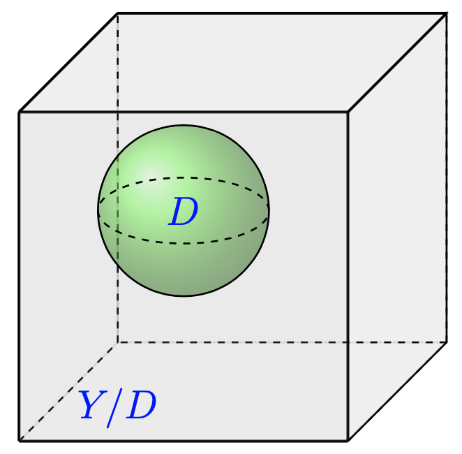
Figure 1. Period cell

The coefficient $a(x)$ is then specified on the unit cell by:

$$a(x)=k\chi_{H}(x)+\chi_{D}(x),$$

where $\chi_{H}$ and $\chi_{D}$ are the indicator functions for the sets $H$ and $D$, and are extended by periodicity to $\mathbb{R}^{3}$. In this paper, we consider periodic crystals made from finite collections of separated inclusions, each with $C^{1,\gamma}$ boundary, where $\gamma>0$.

For each $\alpha\in Y^{\star}$, the Bloch eigenvalues $\xi$ are of finite multiplicity and denoted by $\lambda_{j}(k,\alpha)$, $j\in\mathbb{N}$. We develop power series expansions for each branch of the dispersion relation:

(1.5) $$\lambda_{j}(k,\alpha)=\xi,\,\,\hbox{ $j\in\mathbb{N}$}$$

that are valid for $k$ in a neighborhood of infinity.

To proceed, we complexify the problem and consider $k\in\mathbb{C}$. Now $a(x)$ takes on complex values inside $H$ and the operator $-\nabla\times(k\chi_{H}+\chi_{D})\nabla\times$ is no longer uniformly elliptic. Our approach develops an explicit representation formula for $-\nabla\times(k\chi_{H}+\chi_{D})\nabla\times$ that holds for complex values of $k$. We identify the subset $z={1}/{k}\in\Omega_{0}$ of $\mathbb{C}$ where this operator is invertible. The explicit formula shows that the solution operator $(-\nabla\times(k\chi_{H}+\chi_{D})\nabla\times)^{-1}$ may be regarded more generally as a meromorphic operator valued function of $z$, for $z\in\Omega_{0}=\mathbb{C}\setminus S$, see Section 4 and Lemma 4.1. Here, the set $S$ is discrete and consists of poles lying on the negative real axis with only one accumulation point at $z=-1$. For the problem treated here, we expand about $z=0$, and the distance between $z=0$ and the set $S$ is used to bound the radius of convergence for the power series. The spectral representation for $-\nabla\times(k\chi_{H}+\chi_{D})\nabla\times$ follows from the existence of a complete orthonormal set of $\alpha$-quasiperiodic functions associated with the $\alpha$-quasiperiodic resonances of the crystal, i.e., $\alpha$-quasiperiodic functions $\mathbf{v}$ and real eigenvalues $\lambda_{i}(\alpha)$, $i\in\mathbb{N}$, for which:

$$-\nabla\times(\chi_{D})\nabla\times\mathbf{v}=-\lambda_{i}(\alpha)\Delta\mathbf{v}.$$

The collection of these eigenvalues, for $\alpha\in Y^{\ast}$, comprises the structural spectrum of the crystal. The structural spectrum encodes the geometry of the crystal and inclusions independently of dielectric properties. These resonances are shown to be connected to the spectra of Neumann-Poincaré operators associated with $\alpha$-quasiperiodic double layer potentials. The formal definition of the structural spectrum given in terms of the Neumann-Poincaré eigenvalues, for $\alpha\in Y^{\ast}$, is provided in Definition 2.11.

For $\alpha=\mathbf{0}$, these eigenvalues are the well known electrostatic resonances identified in [6], [5], [27], and [28]. Other electrostatic resonances for a vectorial Helmholtz equation are introduced and explored in [9]. Both Neumann-Poincaré operators and the associated electrostatic resonances have been the focus of theoretical investigations [17], [21] and applied in analysis of plasmonic excitations for suspensions of noble metal particles [26] and electrostatic breakdown [4]. The explicit spectral representation for the operator $-\nabla\times(k\chi_{H}+\chi_{D})\nabla\times$ is crucial for elucidating the interaction between the contrast $k$ and the quasiperiodic resonances of the crystal, see Theorem 2.12.

The spectral representation is applied to analytically continue the band structure $\lambda_{j}(k,\alpha)=\xi$, $j\in\mathbb{N}$, $\alpha\in Y^{\star}$ for $k\in\mathbb{N}$ to $\mathbb{C}$, see Theorem 3.1. On setting $z=1/k$, the spectral representation for the inverse operator written as $A_{\alpha}(z)=(-\nabla\times(k\chi_{H}+\chi_{D})\nabla\times)^{-1}$ shows it to be a meromorphic operator valued function of $z=1/k$, see Section 4 and Lemma 4.1. Application of the contour integral formula for spectral projections [32], [18], [19] delivers an analytic representation formula for the band structure, see Section 4. We apply perturbation theory in Section 4, together with a calculation provided in Section 10, to find an explicit formula for the radii of convergence for the power series $\lambda_{j}(k,\alpha)$ about $1/k=0$. The formula shows that the radius of convergence and the separation between different branches of the dispersion relation for any fixed $\alpha\in Y^{\ast}$ are determined by: 1) the distance of the origin to the nearest pole $z^{\ast}$ of $(-\nabla\times(k\chi_{H}+\chi_{D})\nabla\times)^{-1}$, and 2) the separation between distinct eigenvalues in the $z=1/k\rightarrow 0$ limit, see Theorem 7.1 and Theorem 7.2. These theorems provide conditions on the contrast guaranteeing the separation of the $j$-th and $j+1$-th eigenvalue groups that depend explicitly upon $z^{\ast}$, $j\in\mathbb{N}$ and $\alpha\in Y^{\star}$. Error estimates for series truncated after $N$ terms follow directly from the formulation.

The paper is organized as follows: In the next section, we introduce the Hilbert space formulation of the problem and the variational formulation of the quasi-static resonance problem. The completeness of the eigenfunctions associated with the quasi-static spectrum is established and a spectral representation for the operator $-\nabla\times(k\chi_{H}+\chi_{D})\nabla\times$ is obtained. These results are collected and used to continue the frequency band structure into the complex plane, see Theorem 3.1 of Section 3. Spectral perturbation theory [20] is applied to recover the power series expansion for Bloch spectra in Section 4. The leading order spectral theory is developed for quasiperiodic $\alpha\not=0$ and periodic $\alpha=\mathbf{0}$ problems in Section 5 and Section 6, respectively. The main theorems on radius of convergence and separation of spectra, given by Theorem 7.1 and Theorem 7.2, are presented in Section 7. A large class of geometries for which an $\alpha$-independent lower bound on the quasi-static resonances is introduced in Section 8. Explicit formulas for each term of the power series expansion is recovered and expressed in terms of layer potentials in Section 9. The explicit formulas for the convergence radii are derived in Section 10 as well as hands-on proofs of Theorem 7.1, Theorem 7.2 and the explicit error estimates for $N$-th order truncations.

2. Hilbert space setting, quasiperiodic resonances and representation formulas

The space of all $\alpha$-quasiperiodic complex vector valued functions belonging to $L^{2}_{loc}(\mathbb{R}^{3},\mathbb{C}^{3})$ is denoted by $L^{2}_{\#}(\alpha,Y,\mathbb{C}^{3})$ and the $L^{2}$-inner product is defined by:

(2.1) $$(\mathbf{u},\mathbf{v})=\int_{Y}\,\mathbf{u}\cdot\overline{\mathbf{v}}\,dx.$$

For $\mathbf{h}\in L^{2}_{\#}(\alpha,Y,\mathbb{C}^{3})$, its Helmholtz decomposition is given by:

(2.2) $$\mathbf{h}=\nabla h_{\rm pot}+\nabla\times\mathbf{h}_{\rm curl},$$

where $h_{\rm pot}$ is an $\alpha$-quasiperiodic scalar field belonging to $H^{1}_{loc}(\mathbb{R}^{3},\mathbb{C})$ and $\mathbf{h}_{\rm curl}\in L^{2}_{\#}(\alpha,Y,\mathbb{C}^{3})$, with $\nabla\times\mathbf{h}_{\rm curl}\in L^{2}_{\#}(\alpha,Y,\mathbb{C}^{3})$. The subspaces of gradients and curls are orthogonal with respect to the $L^{2}$-inner product (2.1). The Helmholtz decomposition (2.2) is shown in Appendix A.

For $\alpha\neq\mathbf{0}$, the eigenfunctions $\mathbf{h}$ of (1.4) belong to the space $J_{\#}(\alpha,Y,\mathbb{C}^{3})\subset L^{2}_{\#}(\alpha,Y,\mathbb{C}^{3})$ given by:

(2.3) $$J_{\#}(\alpha,Y,\mathbb{C}^{3})=\{\mathbf{h}\in H_{loc}^{1}(\mathbb{R}^{3},\mathbb{C}^{3}):\,\mathbf{h}\text{ is $\alpha$-quasiperiodic on $Y$},\,\,{\rm div}\,\mathbf{h}=0\text{ in }Y\}.$$

A simple calculation, found in Appendix B, shows that, for $\mathbf{h}\in J_{\#}(\alpha,Y,\mathbb{C}^{3})$, we have $\nabla h_{pot}=0$ in (2.2). Hence, $\mathbf{h}=\nabla\times\mathbf{h}_{\rm curl}$ for $\mathbf{h}\in J_{\#}(\alpha,Y,\mathbb{C}^{3})$. Another straightforward calculation, given in Appendix D, delivers the following result:

Theorem 2.1.

For $\mathbf{u}\in J_{\#}(\alpha,Y,\mathbb{C}^{3})$, the null space of $\nabla\times\mathbf{u}$, for $\alpha\not=0$, is $\{0\}$ and the bilinear form given by:

(2.4) $$\langle\mathbf{u},\mathbf{v}\rangle=\int_{Y}\,\nabla\times\mathbf{u}\cdot\nabla\times\overline{\mathbf{v}}\,dx$$

is an inner product on $J_{\#}(\alpha,Y,\mathbb{C}^{3})$, with norm defined by $\|\mathbf{u}\|^{2}=\langle\mathbf{u},\mathbf{u}\rangle$. The space $J_{\#}(\alpha,Y,\mathbb{C}^{3})$ is a Hilbert space under the inner product (2.4), with $J_{\#}(\alpha,Y,\mathbb{C}^{3})\subset W_{\#}^{1}(\alpha,Y,\mathbb{C}^{3})$ and:

$$\int_{Y}\,\nabla\times\mathbf{u}\cdot\nabla\times\overline{\mathbf{v}}\,dx=\int_{Y}\,\nabla\mathbf{u}:\nabla\overline{\mathbf{v}}\,dx$$

for $\mathbf{u},\,\mathbf{v}\in J_{\#}(\alpha,Y,\mathbb{C}^{3})$, where “ $:$” represents the Frobenius inner product (see Appendix C). Moreover, the null space corresponding to the operator on the left hand side of (1.4) is identically zero.

For $\alpha=\mathbf{0}$, one has that $L^{2}_{\#}(0,Y,\mathbb{C}^{3})$ is the space of periodic $L^{2}$- vector fields on $Y$. For this case, $\mathbf{h}\in L^{2}_{\#}(0,Y,\mathbb{C}^{3})$ has the Helmholtz decomposition into $L^{2}$- orthogonal components given by:

(2.5) $$\mathbf{h}=\nabla h_{\rm pot}+\nabla\times\mathbf{h}_{\rm curl}+\mathbf{c},$$

where $h_{\rm pot}$ is a periodic scalar field belonging to $H^{1}_{loc}(\mathbb{R}^{3},\mathbb{C})$, $\mathbf{h}_{\rm curl}\in L^{2}_{\#}(0,Y,\mathbb{C}^{3})$, with $\nabla\times\mathbf{h}_{\rm curl}\in L^{2}_{\#}(0,Y,\mathbb{C}^{3})$, and $\mathbf{c}$ is a constant vector in $\mathbb{C}^{3}$, see Appendix A. For $\alpha=\mathbf{0}$, the eigenfunctions $\mathbf{h}$ for (1.4) belong to the space:

$$\{\mathbf{h}\in H_{loc}^{1}(\mathbb{R}^{3},\mathbb{C}^{3}):\text{$\mathbf{h}$ periodic on $Y$},\,\,\nabla\cdot\mathbf{h}=0\text{ in }Y\}.$$

A simple calculation, given in Appendix B, shows that $\nabla h_{pot}=0$ and $\mathbf{h}=\nabla\times\mathbf{h}_{curl}+\boldsymbol{c}$. We introduce the space $J_{\#}(0,Y,\mathbb{C}^{3})\subset L^{2}_{\#}(0,Y,\mathbb{C}^{3})$ given by:

(2.6) $$J_{\#}(0,Y,\mathbb{C}^{3})=\{\mathbf{h}\in H_{loc}^{1}(\mathbb{R}^{3},\mathbb{C}^{3}):\text{$\mathbf{h}$ is periodic},\,\,\nabla\cdot\mathbf{h}=0\text{ in }Y,\text{ and }\int_{Y}\,\mathbf{h}\,dx=0\}.$$

Theorem 2.2.

For $\mathbf{u}\in J_{\#}(0,Y,\mathbb{C}^{3})$, the null space of $\nabla\times\mathbf{u}$ is $\{0\}$ and the bilinear form:

(2.7) $$\langle\mathbf{u},\mathbf{v}\rangle=\int_{Y}\,\nabla\times\mathbf{u}\cdot\nabla\times\overline{\mathbf{v}}\,dx,$$

is an inner product on $J_{\#}(0,Y,\mathbb{C}^{3})$, with norm defined by $\|\mathbf{u}\|^{2}=\langle\mathbf{u},\mathbf{u}\rangle$. The space $J_{\#}(0,Y,\mathbb{C}^{3})\subset W_{\#}^{1}(0,Y,\mathbb{C}^{3})$ with inner product (2.7) is a Hilbert space and:

$$\int_{Y}\,\nabla\times\mathbf{u}\cdot\nabla\times\overline{\mathbf{v}}\,dx=\int_{Y}\,\nabla\mathbf{u}:\nabla\overline{\mathbf{v}}\,dx$$

for $\mathbf{u},\,\mathbf{v}\in J_{\#}(0,Y,\mathbb{C}^{3})$. Moreover, the null space corresponding to the operator on the left hand side of (1.4), for $\mathbf{h}\in J_{\#}(0,Y,\mathbb{C}^{3})$, is $\{0\}$.

This theorem follows from a calculation given in Appendix D. From now on, we will refer to $J_{\#}(\alpha,Y,\mathbb{C}^{3})$ for all $\alpha\in Y^{\ast}$, with the special choice of $J_{\#}(\alpha,Y,\mathbb{C}^{3})$ for $\alpha=\mathbf{0}$ defined as in (2.6).

The weak form of equation (1.4) is given by:

(2.8) $$\epsilon^{-1}\int_{H}(\nabla\times\mathbf{h})\cdot(\nabla\times\overline{\mathbf{w}})\ dx+\int_{D}(\nabla\times\mathbf{h})\cdot(\nabla\times\overline{\mathbf{w}})\ dx=\xi\int_{Y}\mathbf{h}\cdot\overline{\mathbf{w}}\ dx,$$

for all $\mathbf{w}\in J_{\#}(\alpha,Y,\mathbb{C}^{3})$. We set $k=\epsilon^{-1}$, and the left hand side of (2.8) is given by the sesquilinear form $B_{k}:J_{\#}(\alpha,Y,\mathbb{C}^{3})\times J_{\#}(\alpha,Y,\mathbb{C}^{3})\rightarrow\mathbb{C}$, defined as:

(2.9) $$B_{k}(\mathbf{u,w}):=k\int_{H}(\nabla\times\mathbf{u})\cdot(\nabla\times\overline{\mathbf{w}})\ dx+\int_{D}(\nabla\times\mathbf{u})\cdot(\nabla\times\overline{\mathbf{w}})\ dx.$$

The linear operator $T_{k}^{\alpha}$, associated with the sesquilinear form $B_{k}$, is defined by:

(2.10) $$\langle T_{k}^{\alpha}\mathbf{u},\mathbf{w}\rangle:=B_{k}(\mathbf{u},\mathbf{w}),$$

for all $\mathbf{u}$ and $\mathbf{w}$ in $J_{\#}(\alpha,Y,\mathbb{C}^{3})$.

Our goal is to rewrite (1.4) in terms of a spectral representation formula for the differential operator $\nabla\times\left(k\nabla\times\cdot\right)$. We will do this by developing the spectral representation of $T_{k}^{\alpha}$, which can be directly linked to the following eigenvalue problem:

(2.11) $$\lambda\langle\mathbf{u},\mathbf{w}\rangle=\lambda\int_{Y}(\nabla\times\mathbf{u})\cdot(\nabla\times\overline{\mathbf{w}})\,dx=\int_{D}(\nabla\times\mathbf{u})\cdot(\nabla\times\overline{\mathbf{w}})\,dx,$$

for all $\mathbf{u,w}\in J_{\#}(\alpha,Y,\mathbb{C}^{3})$; which will be shown to possess countably many real eigenvalues $\lambda_{n}$, with corresponding eigenfunctions $\psi_{n}\in J_{\#}(\alpha,Y,\mathbb{C}^{3})$, that satisfy:

$$\lambda_{n}\int_{Y}(\nabla\times\psi_{n})\cdot(\nabla\times\overline{\mathbf{w}})\,dx=\int_{D}(\nabla\times\psi_{n})\cdot(\nabla\times\overline{\mathbf{w}})\,dx,\qquad\forall\mathbf{w}\in J_{\#}(\alpha,Y,\mathbb{C}^{3}).$$

The eigenspaces associated with different eigenvalues are easily seen to be orthogonal in the inner product (2.4). We apply these eigenfunctions to introduce a different decomposition of $J_{\#}(\alpha,Y,\mathbb{C}^{3})$ that is orthogonal in the inner product (2.4). We introduce the three subspaces denoted by $W_{1}^{\alpha}$, $W_{2}^{\alpha}$, $W_{3}^{\alpha}$ that are mutually orthogonal with respect to the inner product (2.4) and defined as:

(2.12) $$W_{1}^{\alpha}=\left\{\mathbf{u}\in J_{\#}(\alpha,Y,\mathbb{C}^{3}),\,\,\nabla\times\mathbf{u}=0\text{ in }D\right\},$$

(2.13) $$W_{2}^{\alpha}=\left\{\mathbf{u}\in J_{\#}(\alpha,Y,\mathbb{C}^{3}),\,\,\nabla\times\mathbf{u}=0\text{ in }H\right\},$$

and $W_{3}^{\alpha}\subset J_{\#}(\alpha,Y,\mathbb{C}^{3})$ is the subspace perpendicular to the direct sum $(W_{1}^{\alpha}\oplus W_{2}^{\alpha})$.

The decomposition of $J_{\#}(\alpha,Y,\mathbb{C}^{3})$ is recorded in the following lemma.

Lemma 2.3.

The space $J_{\#}(\alpha,Y,\mathbb{C}^{3})$ can be decomposed into orthogonal invariant subspaces spanned by eigenfunctions of the eigenvalues of problem (2.11) and:

$$J_{\#}(\alpha,Y,\mathbb{C}^{3})=W_{1}^{\alpha}\oplus W_{2}^{\alpha}\oplus W_{3}^{\alpha}.$$

It follows from the definitions of $W_{1}^{\alpha}$ and $W_{2}^{\alpha}$ that they are subspaces of the eigenspaces of (2.11) associated with the eigenvalues $0$ and $1$, respectively. From (2.11), we easily deduce that the eigenvalues $\lambda$ belong to $[0,1]$. To proceed, we must provide the explicit characterization of functions in $W_{3}$ in terms of eigenspaces. To do this, we introduce the appropriate differential operators defined on the surface of the dielectric inclusion $\partial D$. We begin by defining the surface differential operators for smooth functions. The surface divergence $Div_{S}$ for smooth complex-valued tangential vector fields $\mathbf{v}$ is defined over the surface $\partial D$ by:

$$Div_{S}\mathbf{v}:=\sum_{j,i}n_{i}(n_{i}\partial_{j}-n_{j}\partial_{i})v_{j},$$

where $n_{i},\,i=1,2,3$, are the components of the unit outward normal vector $\mathbf{n}$ to the surface. The operator:

$$\mathbf{n}\cdot\nabla\times\mathbf{v} := (n_{2}\partial_{3}-n_{3}\partial_{2},n_{3}\partial_{1}-n_{1}\partial_{3},n_{1}\partial_{2}-n_{2}\partial_{1})\cdot\mathbf{v}$$

is only composed of tangential derivatives and can be viewed as an operator defined on $\partial D$. For every vector field $\mathbf{v}$ in $L^{2}(\partial D)^{3}$, we have the relation between $Div_{S}$ and $\mathbf{n}\cdot\nabla\times$ given by:

$$Div_{S}(\mathbf{n}\times\mathbf{v})=-\mathbf{n}\cdot\nabla\times\mathbf{v},$$

see [29]. Also, see [29], for a scalar function $f\in W^{s,2}(\partial D)$ and a vector function $\mathbf{g}\in W^{1-s,2}(\partial D)^{3}$, for $0\leq s\leq 1$, we have the identity:

(2.14) $$\begin{split}\int_{\partial D}\mathbf{g}\cdot\mathbf{n}\times\nabla f\,ds=-\int_{\partial D}f(\mathbf{n}\cdot\nabla\times\mathbf{g})\,ds.\end{split}$$

To complete the set up, we introduce the spaces:

$$L^{2}_{t}(\partial D)^{3} \,=\,\left\{\boldsymbol{\rho}\in L^{2}(\partial D)^{3}\middle|\ \ \mathbf{n}\cdot\boldsymbol{\rho}=0\ \ \text{on}\ \ \partial D\right\},$$

$$L^{2}_{t,0}(\partial D)^{3} \,=\,\left\{\boldsymbol{\rho}\in L^{2}_{t}(\partial D)^{3}\middle|\ \ Div_{S}\boldsymbol{\rho}=0\ \ \text{on}\ \ \partial D\right\},$$

$$L^{2}_{0}(\partial D) \,=\,\left\{{\rho}\in L^{2}(\partial D)\middle|\ \ (\rho,1)_{\partial D}=0\right\},$$

$$H^{-1/2}_{0}(\partial D) \,=\,\left\{{\rho}\in H^{-1/2}(\partial D)\middle|\ \ (\rho,1)_{\partial D}=0\right\},$$

where $\displaystyle(\rho,1)_{\partial D}:=\int_{\partial D}\rho\,ds$.

In order to relate $W_{3}^{\alpha}$ to the invariant subspaces of the eigenvalue problem (2.11), we will introduce a representation of $W_{3}^{\alpha}$ given by single layer potentials parameterized by densities on $\partial D$. This is done in the next section.

2.1. Mapping Properties of the Single Layer Potential Operator

We start by introducing the $\alpha$-quasiperiodic Green’s function:

(2.15) $${G^{\alpha}}(x,y)=-\sum_{\mathbf{n}\in\mathbf{Z}^{3}}\dfrac{e^{i(2\pi\mathbf{n}+\alpha)\cdot(x-y)}}{|{\alpha}+2\pi\mathbf{n}|^{2}}I_{3\times 3},\,\,\,\,\hbox{for $\alpha\not=0$},$$

and the periodic Green’s function:

(2.16) $${G^{0}}(x,y)=-\sum_{\mathbf{n}\in\mathbf{Z}^{3}\setminus\{0\}}\dfrac{e^{i(2\pi\mathbf{n})\cdot(x-y)}}{|2\pi\mathbf{n}|^{2}}I_{3\times 3},\,\,\,\,\hbox{for $\alpha=\mathbf{0}$},$$

where $|\cdot|$ is the usual norm of a vector in $\mathbb{R}^{3}$. For $\alpha\in Y^{\ast}$ and $\boldsymbol{\rho}\in L^{2}_{t,0}(\partial D)^{3}$, we define the $\alpha$-quasiperiodic single layer potential as:

(2.17) $$\begin{split}{S^{\alpha}}(\boldsymbol{\rho})(x)=\int_{\partial D}{G^{\alpha}}(x,y)\boldsymbol{\rho}(y)ds_{y},\ \ \ x\not\in\partial D.\end{split}$$

The single layer potential operator satisfies the continuity condition at $x\in\partial D$:

(2.18) $$S^{\alpha}(\boldsymbol{\rho})\big{|}_{\partial D}^{+}=S^{\alpha}(\boldsymbol{\rho})\big{|}_{\partial D}^{-},$$

(2.19) $$-\Delta S^{\alpha}(\boldsymbol{\rho})=0\text{ for $x\in H\cup D$,}$$

and $S^{\alpha}(\boldsymbol{\rho})\in W_{\#}(\alpha,Y,\mathbb{C}^{3})$ with $S^{\alpha}(\boldsymbol{\rho})\big{|}_{\partial D}$ in $W^{1/2,2}(\partial D)^{3}$. Let $\Gamma^{-}(x)$ be a truncated circular cone in the interior of $D$ with vertex $x$ and let $\Gamma^{+}(x)$ be a truncated circular cone in the interior of $H$ with vertex $x$. Now consider these cones with common vertex $\mathbf{p}$ on $\partial D$. The boundary trace of a function $f$ at $\mathbf{p}$, $f(\mathbf{p})\big{|}_{\partial D}^{\pm}$, is given by:

$$\lim_{\stackrel{{\scriptstyle x\rightarrow\mathbf{p}}}{{x\,\in\,\Gamma^{+}(\mathbf{p})}}}f(x)=f(\mathbf{p})\big{|}_{\partial D}^{+}\,\,,\qquad\lim_{\stackrel{{\scriptstyle x\rightarrow\mathbf{p}}}{{x\,\in\,\Gamma^{-}(\mathbf{p})}}}f(x)=f(\mathbf{p})\big{|}_{\partial D}^{-}\,.$$

We introduce the magnetic dipole operator $M^{\alpha}:L^{2}_{t,0}(\partial D)^{3}\rightarrow L^{2}_{t,0}(\partial D)^{3}$ given by:

(2.20) $$M^{\alpha}(\boldsymbol{\rho})=\mathbf{n}\times\left({\rm p.v.}\int_{\partial D}\nabla_{x}\times\left({G}^{\alpha}(x,y)\ \boldsymbol{\rho}(y)\right)ds_{y}\right),\qquad x\in\partial D\text{ and }\alpha\in Y^{*}.$$

We have the following jump conditions for $x\in\partial D$:

(2.21) $$\mathbf{n}\times\nabla_{x}\times S^{\alpha}(\boldsymbol{\rho})\big{|}_{\partial D}^{\pm}=\pm\frac{1}{2}\boldsymbol{\rho}+M^{\alpha}(\boldsymbol{\rho}).$$

For scalar densities $\rho\in L^{2}(\partial D)$, we recall the jump conditions for $x\in\partial D$:

$$\mathbf{n}\cdot\nabla_{x}S^{\alpha}(\rho)\big{|}_{\partial D}^{\pm}=\mp\frac{1}{2}\rho+(K^{-\alpha})^{\ast}(\rho),$$

where the Neumann–Poincaré operator $(K^{-\alpha})^{\ast}$ is defined by:

$$(K^{-\alpha})^{\ast}(\rho)={\rm p.v.}\int_{\partial D}\frac{\partial G^{\alpha}(x,y)}{\partial\mathbf{n}(x)}\rho(y)\,ds_{y}.$$

Applying Lemma 4.2 of [29] we obtain:

$${\rm div}\,S^{\alpha}(\boldsymbol{\rho})(x)=\int_{\partial D}{G^{\alpha}}(x,y)(\text{Div}_{S}^{\alpha}\boldsymbol{\rho}(y))ds_{y},$$

and:

(2.22) $${\rm div}\,S^{\alpha}(\boldsymbol{\rho})(x)=0,$$

since $\boldsymbol{\rho}$ in $L^{2}_{t,0}(\partial D)^{3}$. We may extend Lemma 4.4 of [29] to the periodic and $\alpha$-quasiperiodic cases, see Appendix E, to deliver a commutation relation between the surface divergence, the magnetic dipole and the Neumann–Poincaré operator given by:

(2.23) $${Div}_{S}M^{\alpha}(\boldsymbol{\rho})=(K^{-\alpha})^{\ast}(Div_{S}\boldsymbol{\rho}),$$

where equality holds as elements of $W^{-1}(\partial D)$. It is noted, for future reference, that:

(2.24) $$\boldsymbol{n}\cdot\nabla\times S^{\alpha}(\boldsymbol{\rho})\,:\,L^{2}_{t,0}(\partial D)^{3}\rightarrow L_{0}^{2}(\partial D),$$

is an isomorphism, see [29].

The following two lemmas are crucial for the parametrization of $W_{3}^{\alpha}$ by single layer potentials.

Lemma 2.4.

Let the single layer potential operator $S^{\alpha}$ be defined as in (2.17). For every $\boldsymbol{\rho}\in L^{2}_{t,0}(\partial D)^{3}$, we have that $S^{\alpha}(\boldsymbol{\rho})\in W_{3}^{\alpha}$.

Proof.

First, recall that $[S^{\alpha}(\boldsymbol{\rho})]|_{\partial D}^{\pm}=0$ from (2.18), ${\rm div}S^{\alpha}(\boldsymbol{\rho})=0$ in $Y$ from (2.22), and from (2.19) it follows that:

(2.25) $$\nabla\times\nabla\times S^{\alpha}(\boldsymbol{\rho})=\nabla(\nabla\cdot S^{\alpha}(\boldsymbol{\rho}))-\Delta S^{\alpha}(\boldsymbol{\rho})=-\Delta S^{\alpha}(\boldsymbol{\rho})=0\text{,\,\,\, for $x\in H\cup D$.}$$

Choosing a smooth $\boldsymbol{w}_{2}$ in $W_{2}^{\alpha}$, we get:

(2.26) $$\int_{Y}\,\nabla\times S^{\alpha}(\boldsymbol{\rho})\cdot\nabla\times\overline{\boldsymbol{w}}_{2}\,dx=\int_{D}\,\nabla\times S^{\alpha}(\boldsymbol{\rho})\cdot\nabla\times\overline{\boldsymbol{w}}_{2}\,dx.$$

Since $\boldsymbol{w}_{2}\in W_{2}^{\alpha}$, we have that $\nabla\times\boldsymbol{w}_{2}=0$ in $H$ and, since $H$ is connected, we have $\boldsymbol{w}_{2}=\nabla\phi$ in $H$, for some scalar potential $\phi$, with $\boldsymbol{w}_{2}|_{\partial D}^{-}=\boldsymbol{w}_{2}|_{\partial D}^{+}=\nabla\phi|_{\partial D}^{+}$. Integration by parts in (2.26), the application of (2.25), and the fact that $\boldsymbol{w}_{2}|_{\partial D}^{-}=\nabla\phi|_{\partial D}^{+}$ give:

$$\int_{D}\nabla\times S^{\alpha}(\boldsymbol{\rho})\cdot\nabla\times\overline{\mathbf{w}}_{2}\,dx =\int_{D}\nabla\times\nabla\times S^{\alpha}(\boldsymbol{\rho})\cdot\overline{\mathbf{w}}_{2}\,dx-\int_{\partial D^{-}}\mathbf{n}\times\nabla\times S^{\alpha}(\boldsymbol{\rho})\cdot\overline{\mathbf{w}}_{2}\,ds_{x}$$

(2.27) $$=-\int_{\partial D^{-}}\mathbf{n}\times\nabla\times S^{\alpha}(\boldsymbol{\rho})\cdot\nabla\phi\,ds_{x}$$

and, from (2.21), we see that:

$$\int_{\partial D^{-}}\,\boldsymbol{n}\times\nabla\times S^{\alpha}(\boldsymbol{\rho})\cdot\nabla\phi\,ds_{x} =\int_{\partial D^{-}}\,\left(-\frac{1}{2}\boldsymbol{\rho}+M^{\alpha}(\boldsymbol{\rho})\right)\cdot\nabla\phi\,ds_{x}$$

(2.28) $$=\int_{\partial D^{-}}\,\left(\frac{1}{2}Div_{S}\boldsymbol{\rho}-Div_{S}M^{\alpha}(\boldsymbol{\rho})\right)\phi\,ds_{x}.$$

Since $\boldsymbol{\rho}\in L^{2}_{t,0}(\partial D)^{3}$, from (2.23) we obtain:

(2.29) $${Div}_{S}M^{\alpha}(\boldsymbol{\rho})=(K^{-\alpha})^{\ast}(Div_{S}^{\alpha}(\boldsymbol{\rho})=0.$$

It now follows immediately, from (2.26), (2.27), (2.1) and (2.29), that:

(2.30) $$\int_{Y}\,\nabla\times S^{\alpha}(\boldsymbol{\rho})\cdot\nabla\times\overline{\boldsymbol{w}}_{2}\,dx=0,$$

for a dense set of test fields $\boldsymbol{w}_{2}$ in $W_{2}^{\alpha}$, and we conclude that $S^{\alpha}(\boldsymbol{\rho})\perp W_{2}^{\alpha}$. Identical arguments can be made for $\boldsymbol{w}_{1}\in W_{1}^{\alpha}$, to find that:

$$\int_{Y}\,\nabla\times S^{\alpha}(\boldsymbol{\rho})\cdot\nabla\times\overline{\boldsymbol{w}}_{1}\,dx=0,$$

and the lemma follows. ∎

Define the Sobolev space:

$$V^{{}^{-\frac{1}{2}}}_{t}(\partial D)^{3}:=\left\{(\mathbf{n}\times\nabla)f\ :\ f\in W^{{1}/{2},2}(\partial D)\right\},$$

with the norm $\|A\|_{V^{{}^{-\frac{1}{2}}}_{t}(\partial D)^{3}}$ given by:

$$\|A\|_{V^{{}^{-\frac{1}{2}}}_{t}(\partial D)^{3}}=\text{inf}\left\{\|\sigma+f\|_{W^{{1}/{2},2}(\partial D)}\ :\ \sigma\in\mathbb{C},\ \ f\in W^{\frac{1}{2},2}(\partial D),\ \ (\mathbf{n}\times\nabla)f=A\right\}.$$

Moreover, from [29], we have:

$$L^{2}_{t,0}(\partial D)^{3}=V^{0}_{t}(\partial D)^{3}=\left\{(\mathbf{n}\times\nabla)f\ :\ f\in W^{1,2}(\partial D)\right\},$$

with:

(2.31) $$\mathbf{n}\times\nabla :W^{1,2}(\partial D)\setminus\mathbb{C}\rightarrow L^{2}_{t,0}(\partial D)^{3},$$

(2.32) $$\mathbf{n}\times\nabla :W^{1/2,2}(\partial D)\setminus\mathbb{C}\rightarrow V^{{}^{-\frac{1}{2}}}_{t}(\partial D)^{3},$$

isomorphisms, and:

$$L^{2}_{t,0}(\partial D)^{3}\subset V^{{}^{-\frac{1}{2}}}_{t}(\partial D)^{3}\subset W^{-{1}/{2},2}(\partial D)^{3}.$$

We now present the mapping property of the single layer potential operator necessary for characterizing the spectrum of the sesquilinear operator $T^{\alpha}=S^{\alpha}M^{\alpha}(S^{\alpha})^{-1}$.

Theorem 2.5.

The single layer potential operator can be extended as a bounded linear map from $V^{{}^{-\frac{1}{2}}}_{t}(\partial D)^{3}$ to $W_{3}^{\alpha}$.

Proof.

To prove this theorem, we first show the following lemma.

Lemma 2.6.

The space of tangential vector fields $L^{2}_{t,0}(\partial D)^{3}$ is a dense subspace of $V^{{}^{-\frac{1}{2}}}_{t}(\partial D)^{3}$.

Proof.

Note that, from (2.32), for ${\boldsymbol{g}}\in V^{{}^{-\frac{1}{2}}}_{t}(\partial D)^{3}$ we can write ${\boldsymbol{g}}=\mathbf{n}\times\nabla f$, for some $f\in W^{1/2,2}(\partial D)\setminus\mathbb{C}$. From the density of $W^{1,2}(\partial D)$ in $W^{1/2,2}(\partial D)$, there exists a sequence $\left\{f_{j}\right\}_{j=1}^{\infty}\in W^{1,2}(\partial D)^{2}\setminus\mathbb{C}\ \subset\ W^{1/2,2}(\partial D)\setminus\mathbb{C}$ converging to $f$ in $W^{1/2,2}(\partial D)\setminus\mathbb{C}$. From (2.31), there are associated functions ${\boldsymbol{g}}_{j}$ in $L^{2}_{t,0}(\partial D)^{3}$ such that ${\boldsymbol{g}}_{j}={\boldsymbol{n}}\times\nabla f_{j}$. By the continuity of the map $\mathbf{n}\times\nabla:W^{1/2,2}(\partial D)\rightarrow V^{{}^{-\frac{1}{2}}}_{t}(\partial D)^{3}$, we have the existence of a positive constant $C$ such that:

$$\|{\boldsymbol{g}}-{\boldsymbol{g}}_{j}\|_{V^{-\frac{1}{2}}_{t}(\partial D)}=\|\mathbf{n}\times\nabla f-\mathbf{n}\times\nabla f_{j}\|_{V^{-\frac{1}{2}}_{t}(\partial D)}\leq C\|f-f_{j}\|_{W^{1/2,2}(\partial D)\setminus\mathbb{C}}\,,$$

and it follows that $L^{2}_{t,0}(\partial D)^{3}$ is dense in $V^{{}^{-\frac{1}{2}}}_{t}(\partial D)^{3}.$ ∎

With Lemma 2.6 in hand, we prove Theorem 2.5. Given ${\boldsymbol{\rho}}\in L^{2}_{t,0}(\partial D)^{3}$ and $S^{\alpha}({\boldsymbol{\rho}})\in W_{3}^{\alpha}$, we have:

(2.33) $$\|S^{\alpha}({\boldsymbol{\rho}})\|^{2} =\int_{H}\nabla\times S^{\alpha}({\boldsymbol{\rho}})\cdot\nabla\times\overline{S^{\alpha}({\boldsymbol{\rho}})}\,d\mathbf{x}+\int_{D}\nabla\times S^{\alpha}({\boldsymbol{\rho}})\cdot\nabla\times\overline{S^{\alpha}({\boldsymbol{\rho}})}\,d\mathbf{x}$$

$$=\int_{\partial D}[\mathbf{n}\times\nabla\times S^{\alpha}({\boldsymbol{\rho}})]^{-}_{+}\cdot\ \overline{S^{\alpha}({\boldsymbol{\rho}})}\,ds_{\mathbf{x}}$$

$$=-\int_{\partial D}{\boldsymbol{\rho}}\cdot\ \overline{S^{\alpha}({\boldsymbol{\rho}})}\,ds_{\mathbf{x}}.$$

Writing ${\boldsymbol{\rho}}=\mathbf{n}\times\nabla f$, for $f\in W^{1,2}(\partial D)\setminus\mathbb{C}$, and using (2.14) in (2.33), we get:

$$-\int_{\partial D}{\boldsymbol{\rho}}\ \cdot\overline{S^{\alpha}({\boldsymbol{\rho}})}\,ds_{\mathbf{x}}=-\int_{\partial D}\mathbf{n}\times\nabla f\cdot\ \overline{S^{\alpha}({\boldsymbol{\rho}})}\,ds_{\mathbf{x}}=\int_{\partial D}f\ \mathbf{n}\cdot\nabla\times\overline{S^{\alpha}({\boldsymbol{\rho}})}\,ds_{\mathbf{x}}.$$

From (2.24), $\mathbf{n}\cdot\nabla\times S^{\alpha}({\boldsymbol{\rho}})\in L^{2}_{0}(\partial D)$, so it also belongs to $W^{-\frac{1}{2},2}_{0}(\partial D)=(W^{\frac{1}{2},2}(\partial D)\setminus\mathbb{C})^{\prime}$, where the notation “ ^′ ” is used to indicate the dual space. From (2.33) and the last equation above, for $f\in W^{{1,2}}(\partial D)\setminus\mathbb{C}$, we have:

$$\|S^{\alpha}({\boldsymbol{\rho}})\|^{2}=\int_{\partial D}f\ \mathbf{n}\cdot\nabla\times\overline{S^{\alpha}({\boldsymbol{\rho}})}\,ds_{\mathbf{x}}\leq\inf_{\sigma\in\mathbb{C}}\|f+\sigma\|_{W^{\frac{1}{2},2}(\partial D)}\|\mathbf{n}\cdot\nabla\times S^{\alpha}({\boldsymbol{\rho}})\|_{W^{-\frac{1}{2},2}_{0}(\partial D)}\,,$$

where $\inf_{\sigma\in\mathbb{C}}\|f+\sigma\|_{W^{\frac{1}{2},2}(\partial D)}$ is the norm for $W^{{1,2}}(\partial D)\setminus\mathbb{C}$. Since the map $\mathbf{n}\cdot\nabla\times S^{\alpha}:V^{{}^{-\frac{1}{2}}}_{t}(\partial D)^{3}\rightarrow W^{-\frac{1}{2},2}_{0}(\partial D)$ is bounded (see [29]), we have that $\|\mathbf{n}\cdot\nabla\times S^{\alpha}(\boldsymbol{\rho})\|_{W^{-\frac{1}{2},2}(\partial D)}\leq C\|\boldsymbol{\rho}\|_{V^{{}^{-\frac{1}{2}}}_{t}(\partial D)^{3}}$ and also $\inf_{\sigma\in\mathbb{C}}\|f+\sigma\|_{W^{\frac{1}{2},2}(\partial D)}=\|\boldsymbol{\rho}\|_{V^{-\frac{1}{2}}(\partial D)^{3}}$, so it follows that:

$$\|S^{\alpha}({\boldsymbol{\rho}})\|^{2}\leq C\inf_{\sigma\in\mathbb{C}}\|f+\sigma\|_{W^{\frac{1}{2},2}(\partial D)}\|{\boldsymbol{\rho}}\|_{V^{-\frac{1}{2}}_{t}(\partial D)^{3}}\leq C\|{\boldsymbol{\rho}}\|_{V^{-\frac{1}{2}}_{t}(\partial D)^{3}}^{2}$$

and, therefore:

(2.34) $$\|S^{\alpha}({\boldsymbol{\rho}})\|\leq C\|{\boldsymbol{\rho}}\|_{V^{-\frac{1}{2}}_{t}(\partial D)^{3}}.$$

The inequality (2.34) implies that $S^{\alpha}(\boldsymbol{\rho})$ is a bounded operator mapping into $W_{3}^{\alpha}$ for the densely defined subspace $L^{2}_{t,0}(\partial D)^{3}$ of $V^{{}^{-\frac{1}{2}}}_{t}(\partial D)^{3}$. Then, we extend the densely defined map $S^{\alpha}$ to $V_{t}^{\frac{1}{2}}(\partial D)^{3}$, using the BLT theorem, to deduce that its extension $S^{\alpha}:V^{{}^{-\frac{1}{2}}}_{t}(\partial D)^{3}\rightarrow W_{3}^{\alpha}$ is bounded. ∎

Theorem 2.7.

The single layer potential operator $S^{\alpha}:V^{{}^{-\frac{1}{2}}}_{t}(\partial D)^{3}\rightarrow W_{3}^{\alpha}$ is a bijection.

Proof.

We first show that $S^{\alpha}$ is one-to-one. For a given $\boldsymbol{\rho}\in V^{{}^{-\frac{1}{2}}}_{t}(\partial D)^{3}$, we have $\mathbf{u}=S^{\alpha}(\boldsymbol{\rho})\in W_{3}^{\alpha}$. Furthermore:

$$\begin{split}\boldsymbol{\rho}&=\mathbf{n}\times\nabla\times\mathbf{u}\big{|}_{\partial D^{+}}-\mathbf{n}\times\nabla\times\mathbf{u}\big{|}_{\partial D^{-}}+\mathbf{n}\times\nabla\times\mathbf{u}\big{|}_{\partial Y}-\mathbf{n}\times\nabla\times\mathbf{u}\big{|}_{\partial Y}\\ &=\mathbf{n}\times\nabla\times\mathbf{u}\big{|}_{\partial H}-\mathbf{n}\times\nabla\times\mathbf{u}\big{|}_{\partial D^{-}}-\mathbf{n}\times\nabla\times\mathbf{u}\big{|}_{\partial Y}.\end{split}$$

Given a bounded Lipschitz domain $\Omega\in\mathbb{R}^{3}$, if $\mathbf{f}\in L^{2}(\Omega)^{3}$ and $\nabla\times\mathbf{f}\in L^{2}(\Omega)^{3}$, then $\mathbf{n}\times\mathbf{f}\in W^{-\frac{1}{2},2}(\partial\Omega)^{3}$. As a consequence, there is a $C>0$, depending only on $\partial\Omega$, such that:

$$\|\mathbf{n}\times\mathbf{f}\|_{W^{-\frac{1}{2},2}(\partial\Omega)^{3}}\leq C(\|\mathbf{f}\|_{L^{2}(\Omega)^{3}}+\|\nabla\times\mathbf{f}\|_{L^{2}(\Omega)^{3}}).$$

Set $\mathbf{f}=\nabla\times\mathbf{u}$ and, since $\nabla\times\nabla\times\mathbf{u}=0$ in $H\cup D$, $\boldsymbol{\rho}\in V^{{}^{-\frac{1}{2}}}_{t}(\partial D)^{3}\subset W^{-\frac{1}{2},2}(\partial D)^{3}$, one has:

$$\begin{split}&\|\boldsymbol{\rho}\|_{W^{-\frac{1}{2},2}(\partial D)^{3}}\\ &=\|\mathbf{n}\times\nabla\times\mathbf{u}\big{|}_{\partial D^{+}}-\mathbf{n}\times\nabla\times\mathbf{u}\big{|}_{\partial D^{-}}\|_{W^{-\frac{1}{2},2}(\partial D)^{3}}\\ &\leq\|\mathbf{n}\times\nabla\times\mathbf{u}\|_{W^{-\frac{1}{2},2}(\partial H)^{3}}+\|\mathbf{n}\times\nabla\times\mathbf{u}\|_{W^{-\frac{1}{2},2}(\partial D)^{3}}+\|\mathbf{n}\times\nabla\times\mathbf{u}\|_{W^{-\frac{1}{2},2}(\partial(Y))^{3}}\\ &\leq C(\|\nabla\times\mathbf{u}\|_{L^{2}(H)^{3}}+\|\nabla\times\mathbf{u}\|_{L^{2}(D)^{3}}+\|\nabla\times\mathbf{u}\|_{L^{2}(Y)^{3}})\\ &\leq C\|\mathbf{u}\|=C\|S^{\alpha}(\boldsymbol{\rho})\|.\end{split}$$

Now, for $\boldsymbol{\rho}_{1},\boldsymbol{\rho}_{2}\in V^{{}^{-\frac{1}{2}}}_{t}(\partial D)^{3}\subset W^{-\frac{1}{2},2}(\partial D)^{3}$, we obtain:

$$0\leq\|\boldsymbol{\rho}_{1}-\boldsymbol{\rho}_{2}\|_{W^{-\frac{1}{2},2}(\partial D)^{3}}\leq C_{2}\|S^{\alpha}(\boldsymbol{\rho}_{1})-S^{\alpha}(\boldsymbol{\rho}_{2})\|,$$

to conclude that $S^{\alpha}:V^{{}^{-\frac{1}{2}}}_{t}(\partial D)^{3}\rightarrow W_{3}^{\alpha}$ is one-to-one.

To show the surjectivity of $S^{\alpha}$, assume that $\mathbf{u}\in W_{3}^{\alpha}$ is given. From the definition of $W_{3}^{\alpha}$ and integration by parts, we have:

$$\nabla\cdot\mathbf{u}=0,\quad\quad\nabla\times\nabla\times\mathbf{u}=0,\text{ on $H\cup D$}.$$

Writing ${\mathbf{w}}=\nabla\times\mathbf{u}$, we see that $\nabla\times\mathbf{w}=0$ in $H\cup D$ so $\mathbf{w}=\nabla q_{1}$, for $q_{1}\in W^{1,2}(H)$, and $\mathbf{w}=\nabla q_{2}$, for $q_{2}\in W^{1,2}(D)$. Let $\Gamma^{-}(x)$ be a truncated circular cone in the interior of $D$ with vertex $x$ and let $\Gamma^{+}(x)$ be a truncated circular cone in the interior of $H$ with vertex $x$. Now consider these cones with common vertex $\mathbf{p}$ on $\partial D$. Taking the cross product of $\mathbf{w}=\nabla\times\mathbf{u}$ with the normal to the surface $\partial D$ given by $\mathbf{n}(\mathbf{p})$, we get:

$$\lim_{\stackrel{{\scriptstyle x\rightarrow\mathbf{p}}}{{x\,\in\,\Gamma^{+}(\mathbf{p})}}}\mathbf{n}(\mathbf{p})\times\nabla\times\mathbf{u}(x)=\mathbf{n}(\mathbf{p})\times\nabla q_{1}(\mathbf{p}),\qquad\lim_{\stackrel{{\scriptstyle x\rightarrow\mathbf{p}}}{{x\,\in\,\Gamma^{-}(\mathbf{p})}}}\mathbf{n}(\mathbf{p})\times\nabla\times\mathbf{u}(x)=\mathbf{n}(\mathbf{p})\times\nabla q_{2}(\mathbf{p}).$$

From (2.32), we have that $\mathbf{n}\times\nabla:W^{\frac{1}{2},2}(\partial D)/\mathbb{C}\rightarrow V^{-\frac{1}{2}}_{t}(\partial D)^{3}$ is an isomorphism, and we choose:

$${\boldsymbol{\rho}}_{\mathbf{u}}=\mathbf{n}\times\nabla q_{1}\big{|}_{\partial D^{+}}-\mathbf{n}\times\nabla q_{2}\big{|}_{\partial D^{-}}\,\,\,\in V^{-\frac{1}{2}}(\partial D)^{3}.$$

Setting $\mathbf{v}=S^{\alpha}({\boldsymbol{\rho}}_{\mathbf{u}})$ gives:

(2.35) $$\nabla\times\nabla\times\mathbf{v}=0\ \ \text{in}\ \ D\cup H,\qquad\nabla\cdot\mathbf{v}=0\ \ \text{ in}\ \ Y,\qquad[\mathbf{n}\times\nabla\times\mathbf{v}]^{+}_{-}={\boldsymbol{\rho}}_{\mathbf{u}},$$

and:

(2.36) $$\int_{\partial Y}\,\mathbf{n}\times\nabla\times(\mathbf{v}-\mathbf{u})\cdot(\overline{\mathbf{v}}-\overline{\mathbf{u}})\,ds=0,\qquad\hbox{for $\mathbf{v},\mathbf{u}\in W_{3}^{\alpha}$}.$$

Using integration by parts and applying (2.35) and (2.36), we discover:

$$\|\mathbf{v}-\mathbf{u}\|=0.$$

For $\alpha\not=0$, this implies $\mathbf{v}=\mathbf{u}$ and, for $\alpha=\mathbf{0}$, we have $\mathbf{u}-\mathbf{v}=\mathbf{c}$, where $\mathbf{c}$ is a constant vector. But, for $\alpha=\mathbf{0}$, we have $\displaystyle 0=\int_{Y}\mathbf{w}\ dx=\int_{Y}\mathbf{u}\ dx$, to conclude $\mathbf{c}=0$ and $\mathbf{v}=\mathbf{u}$. This shows that $S^{\alpha}$ is surjective. ∎

From Theorem 2.7, we see that the inverse map $(S^{\alpha})^{-1}\,:W_{3}^{\alpha}\rightarrow{V^{\frac{1}{2}}_{t}}(\partial D)^{3}$ exists. Finally, we apply the open mapping theorem to derive the following theorem.

Theorem 2.8.

The inverse $(S^{\alpha})^{-1}\,:W_{3}^{\alpha}\rightarrow V_{t}^{\frac{1}{2}}(\partial D)^{3}$ is bounded.

2.2. Compactness of Magnetic Dipole Operator

In this section, we show that the magnetic dipole operator $M^{\alpha}$ is compact.

Theorem 2.9.

The operator $M^{\alpha}:V^{{}^{-\frac{1}{2}}}_{t}(\partial D)^{3}\rightarrow V^{{}^{-\frac{1}{2}}}_{t}(\partial D)^{3}$ is compact and satisfies:

(2.37) $$\sigma(M^{\alpha};\ V^{{}^{-\frac{1}{2}}}_{t}(\partial D)^{3})=\sigma((K^{-\alpha})^{\ast};\ H^{-\frac{1}{2}}_{0}(\partial D)),$$

where $(K^{-\alpha})^{\ast}$ is the scalar valued Neumann–Poincaré operator defined on $H^{-\frac{1}{2}}_{0}(\partial D)$ and where $\sigma(M^{\alpha};\ V^{{}^{-\frac{1}{2}}}_{t}(\partial D)^{3})$ and $\sigma((K^{-\alpha})^{\ast};\ H^{-\frac{1}{2}}_{0}(\partial D))$ are the spectra of $M^{\alpha}$ and $(K^{-\alpha})^{\ast}$, respectively.

Proof.

We first establish that the magnetic dipole operator $M^{\alpha}$ is a bounded map of $V^{{}^{-\frac{1}{2}}}_{t}(\partial D)^{3}$. To do this, we start with the following Plemelj-like identity, that can be derived as in[29]:

(2.38) $$(K^{-\alpha})^{\ast}(\mathbf{n}\cdot\nabla\times S^{\alpha})=\mathbf{n}\cdot\nabla\times S^{\alpha}M^{\alpha},\qquad\text{for}\ \ \boldsymbol{\rho}\in L^{2}_{t,0}(\partial D)^{3},$$

The scalar valued Neumann–Poincaré operator is bounded and compact on $H^{-\frac{1}{2}}_{0}(\partial D)$, see [21]. The map $\mathbf{n}\cdot\nabla\times S^{\alpha}:V^{{}^{-\frac{1}{2}}}_{t}(\partial D)^{3}\rightarrow H^{-\frac{1}{2}}_{0}(\partial D)$ can be shown to be an isomorphism, as in [29]. The boundedness of $(K^{-\alpha})^{\ast}$ and the boundedness of the operator $\mathbf{n}\cdot\nabla\times S^{\alpha}$ imply that:

(2.39) $$\begin{split}\|(K^{-\alpha})^{\ast}(\mathbf{n}\cdot\nabla\times S^{\alpha}(\boldsymbol{\rho}))\|_{H^{-\frac{1}{2}}_{0}(\partial D)}&\leq C\|\mathbf{n}\cdot\nabla\times S^{\alpha}(\boldsymbol{\rho})\|_{H^{-\frac{1}{2}}_{0}(\partial D)}\leq C\|\boldsymbol{\rho}\|_{V^{{}^{-\frac{1}{2}}}_{t}(\partial D)^{3}}.\end{split}$$

On the other hand, the boundedness of $\mathbf{n}\cdot\nabla\times S^{\alpha}$ also implies the following:

(2.40) $$\|M^{\alpha}(\boldsymbol{\rho})\|_{V^{{}^{-\frac{1}{2}}}_{t}(\partial D)^{3}}\leq C\|\mathbf{n}\cdot\nabla\times S^{\alpha}M^{\alpha}(\boldsymbol{\rho})\|_{H^{-\frac{1}{2}}_{0}(\partial D)}.$$

In view of (2.38), (2.39), and (2.40), we have:

$$\|M^{\alpha}(\boldsymbol{\rho})\|_{V^{{}^{-\frac{1}{2}}}_{t}(\partial D)^{3}}\leq C\|\boldsymbol{\rho}\|_{V^{{}^{-\frac{1}{2}}}_{t}(\partial D)^{3}},$$

and we conclude that $M^{\alpha}(\boldsymbol{\rho})$ is bounded, for $\boldsymbol{\rho}\in L^{2}_{t,0}(\partial D)^{3}\subset V^{{}^{-\frac{1}{2}}}_{t}(\partial D)^{3}$. Since $L^{2}_{t,0}(\partial D)^{3}$ is dense in $V^{{}^{-\frac{1}{2}}}_{t}(\partial D)^{3}$, we can extend $M^{\alpha}$ as a bounded linear map of $V^{{}^{-\frac{1}{2}}}_{t}(\partial D)^{3}$.

Next, observe that $\mathbf{n}\cdot\nabla\times S^{\alpha}:V^{{}^{-\frac{1}{2}}}_{t}(\partial D)^{3}\rightarrow H^{-\frac{1}{2}}_{0}(\partial D)$ is an isomorphism, so for a bounded sequence $\left\{\boldsymbol{\rho}_{n}\right\}\in V^{{}^{-\frac{1}{2}}}_{t}(\partial D)^{3}$, we have:

$$\|\mathbf{n}\cdot\nabla\times S^{\alpha}(\boldsymbol{\rho}_{n})\|_{H^{-\frac{1}{2}}_{0}(\partial D)}\leq C\|\boldsymbol{\rho}_{n}\|_{V^{{}^{-\frac{1}{2}}}_{t}(\partial D)^{3}},$$

which shows that $\left\{\mathbf{n}\cdot\nabla\times S^{\alpha}(\boldsymbol{\rho}_{n})\right\}_{n=1}^{\infty}\in H^{-\frac{1}{2}}_{0}(\partial D)$ is bounded. By the compactness of $(K^{-\alpha})^{*}$, we have that the subsequence $\left\{(K^{-\alpha})^{*}(\mathbf{n}\cdot\nabla\times S^{\alpha}(\boldsymbol{\rho}_{n_{k}}))\right\}_{k=1}^{\infty}\in H^{-\frac{1}{2}}_{0}(\partial D)$ is Cauchy, which in turn, by (2.38), implies that $\left\{\mathbf{n}\cdot\nabla\times S^{\alpha}(M^{\alpha}(\boldsymbol{\rho}_{n_{k}}))\right\}_{k=1}^{\infty}\in H^{-\frac{1}{2}}_{0}(\partial D)$ is also Cauchy. Because $\mathbf{n}\cdot\nabla\times S^{\alpha}:V^{{}^{-\frac{1}{2}}}_{t}(\partial D)^{3}\rightarrow H^{-\frac{1}{2}}_{0}(\partial D)$ is an isomorphism and $(K^{\alpha})^{*}$ is a continuous map, we have for $\{\boldsymbol{\rho}_{n_{k}}\}_{k=1}^{\infty}$:

$$\|M^{\alpha}(\boldsymbol{\rho}_{n_{k}})-M^{\alpha}(\boldsymbol{\rho}_{n_{l}})\|_{V^{{}^{-\frac{1}{2}}}_{t}(\partial D)^{3}}\\ \leq C\|\mathbf{n}\cdot\nabla\times S^{\alpha}(M^{\alpha}(\boldsymbol{\rho}_{n_{k}}))-\mathbf{n}\cdot\nabla\times S^{\alpha}(M^{\alpha}(\boldsymbol{\rho}_{n_{l}}))\|_{H^{-\frac{1}{2}}_{0}(\partial D)}\,,$$

and we conclude that the sequence $\left\{M^{\alpha}(\boldsymbol{\rho}_{n_{k}})\right\}_{n=1}^{\infty}\in V^{{}^{-\frac{1}{2}}}_{t}(\partial D)^{3}$ is Cauchy, and thus, $M^{\alpha}$ is a compact operator on $V^{{}^{-\frac{1}{2}}}_{t}(\partial D)^{3}$. Finally, the identity (2.37) is the direct consequence of (2.38), and the isomorphic map $\mathbf{n}\cdot\nabla\times S^{\alpha}:V^{{}^{-\frac{1}{2}}}_{t}(\partial D)^{3}\rightarrow H^{-\frac{1}{2}}_{0}(\partial D)$. ∎

It is noted that the spectrum of $(K^{-\alpha})^{*}$ lies in $[-1/2,1/2]$ (see e.g., [21]) and, by the previous theorem, we see that:

(2.41) $$\sigma(M^{\alpha};\ V^{{}^{-\frac{1}{2}}}_{t}(\partial D)^{3})\subset[-1/2,1/2].$$

2.3. Spectral Property of the operator $T^{\alpha}=S^{\alpha}M^{\alpha}(S^{\alpha})^{-1}$

Theorem 2.10.

The operator $T^{\alpha}=S^{\alpha}M^{\alpha}(S^{\alpha})^{-1}:W_{3}^{\alpha}\rightarrow W_{3}^{\alpha}$ is Hermitian, compact, and satisfies:

(2.42) $$\sigma\left(T^{\alpha};\ W_{3}^{\alpha}\right)=\sigma(M^{\alpha};\ V^{{}^{-\frac{1}{2}}}_{t}(\partial D)^{3}).$$

Proof.

First, we show that $T^{\alpha}:W_{3}^{\alpha}\rightarrow W_{3}^{\alpha}$ is Hermitian. For $\mathbf{u},\,\mathbf{w}\in W_{3}^{\alpha}$, we have:

$$\begin{split}\langle T^{\alpha}\mathbf{u},\mathbf{w}\rangle&=\int_{Y}(\nabla\times S^{\alpha}M^{\alpha}(S^{\alpha})^{-1}\mathbf{u})\cdot(\nabla\times\overline{\mathbf{w}})\ dx\\ &=\int_{H}(\nabla\times S^{\alpha}M^{\alpha}(S^{\alpha})^{-1}\mathbf{u})\cdot(\nabla\times\overline{\mathbf{w}})\ dx+\int_{D}(\nabla\times S^{\alpha}M^{\alpha}(S^{\alpha})^{-1}\mathbf{u})\cdot(\nabla\times\overline{\mathbf{w}})\ dx.\end{split}$$

Using integration by parts and since $\nabla\times\nabla\times S^{\alpha}M^{\alpha}(S^{\alpha})^{-1}\mathbf{u})=0$ in $H\cup D$, we see that:

$$\int_{Y}(\nabla\times S^{\alpha}M^{\alpha}(S^{\alpha})^{-1}\mathbf{u})\cdot(\nabla\times\overline{\mathbf{w}})\ dx=\int_{\partial D}\left[\mathbf{n}\times\nabla\times S^{\alpha}M^{\alpha}(S^{\alpha})^{-1}\mathbf{u}\right]^{+}_{-}\cdot\overline{\mathbf{w}}\ ds_{\mathbf{x}}.$$

Then, using the jump condition (2.21), we obtain $\langle T^{\alpha}\mathbf{u},\mathbf{w}\rangle=\int_{\partial D}M^{\alpha}(S^{\alpha})^{-1}\mathbf{u}\cdot\overline{\mathbf{w}}\ ds_{\mathbf{x}}$. We can write $\mathbf{u}=S^{\alpha}\boldsymbol{\beta}$, for some $\boldsymbol{\beta}\in V^{{}^{-\frac{1}{2}}}_{t}(\partial D)^{3}$, to get:

$$\begin{split}\langle T^{\alpha}\mathbf{u},\mathbf{w}\rangle&=\int_{\partial D}M^{\alpha}\boldsymbol{\beta}\cdot\overline{\mathbf{w}}\ ds_{x}\\ &=\dfrac{1}{2}\int_{\partial D}[\mathbf{n}\times\nabla\times S^{\alpha}\boldsymbol{\beta}\big{|}_{+}-\mathbf{n}\times\nabla\times S^{\alpha}\boldsymbol{\beta}\big{|}_{-}]\cdot\overline{\mathbf{w}}\ ds_{x}.\end{split}$$

Integration by parts gives:

$$\begin{split}&\dfrac{1}{2}\int_{\partial D}[\mathbf{n}\times\nabla\times S^{\alpha}\boldsymbol{\beta}\big{|}_{+}-\mathbf{n}\times\nabla\times S^{\alpha}\boldsymbol{\beta}\big{|}_{-}]\cdot\overline{\mathbf{w}}\ ds_{x}\\ &=\dfrac{1}{2}\int_{H}(\nabla\times S^{\alpha}\boldsymbol{\beta})\cdot(\nabla\times\overline{\mathbf{w}})\ dx-\dfrac{1}{2}\int_{D}(\nabla\times S^{\alpha}\boldsymbol{\beta})\cdot(\nabla\times\overline{\mathbf{w}})\ dx.\end{split}$$

Therefore:

(2.43) $$\langle T^{\alpha}\mathbf{u},\mathbf{w}\rangle=\dfrac{1}{2}\int_{H}(\nabla\times\mathbf{u})\cdot(\nabla\times\overline{\mathbf{w}})\ dx-\dfrac{1}{2}\int_{D}(\nabla\times\mathbf{u})\cdot(\nabla\times\overline{\mathbf{w}})\ dx,$$

and $T^{\alpha}$ is seen to be Hermitian.

Now, the identity given by (2.42) is established. Consider the eigenvalue eigenvector pair $(\mu,\boldsymbol{\rho})\in\sigma\left(M^{\alpha};\ V^{{}^{-\frac{1}{2}}}_{t}(\partial D)^{3}\right)\times V^{{}^{-\frac{1}{2}}}_{t}(\partial D)^{3}$ of $M^{\alpha}\boldsymbol{\rho}=\mu\boldsymbol{\rho}$. There exists $\mathbf{u}\in W_{3}^{\alpha}$ such that $\mathbf{u}=S^{\alpha}\boldsymbol{\rho}$, and $\boldsymbol{\rho}=(S^{\alpha})^{-1}\mathbf{u}$. Therefore, we have $M^{\alpha}(S^{\alpha})^{-1}\mathbf{u}=\mu S^{-1}\mathbf{u}$. This implies that:

$$S^{\alpha}M^{\alpha}(S^{\alpha})^{-1}\mathbf{u}=\mu S^{\alpha}(S^{\alpha})^{-1}\mathbf{u}\ \ \Rightarrow\ \ \ T^{\alpha}\mathbf{u}=\mu\mathbf{u},$$

which shows that $\sigma\left(M^{\alpha};\ V^{{}^{-\frac{1}{2}}}_{t}(\partial D)^{3}\right)\subset\sigma\left(T^{\alpha};\ W_{3}^{\alpha}\right)$.

On the other hand, if we have $T^{\alpha}\mathbf{u}=\mu\mathbf{u}$, then $S^{\alpha}M^{\alpha}(S^{\alpha})^{-1}\mathbf{u}=\mu\mathbf{u}$; therefore, multiplying both sides by $(S^{\alpha})^{-1}$ gives $M^{\alpha}(S^{\alpha})^{-1}\mathbf{u}=\mu(S^{\alpha})^{-1}\mathbf{u}$, and we obtain:

$$\sigma\left(T^{\alpha};\ W_{3}^{\alpha}\right)\subset\sigma(M^{\alpha};\ V^{{}^{-\frac{1}{2}}}_{t}(\partial D)^{3}).$$

Finally, the compactness of $T^{\alpha}=S^{\alpha}M^{\alpha}(S^{\alpha})^{-1}$ easily follows from the compactness of $M^{\alpha}$. ∎

It now follows from (2.43) that the eigenvalue problem $T^{\alpha}\boldsymbol{u}=\mu\boldsymbol{u}$ is equivalent to (2.11), so the eigenfunctions form a complete orthonormal system that span $W_{3}^{\alpha}$.

It is clear from Theorems 2.9 and 2.10 that:

$$\sigma\left(T^{\alpha};\ W_{3}^{\alpha}\right)=\sigma((K^{-\alpha})^{*};\ H^{-\frac{1}{2}}_{0}(\partial D)),$$

and we denote dependence on $\alpha$ explicitly and write $\mu_{i}(\alpha)$, $i\in\mathbb{N}$, $\alpha\in Y^{\ast}$ and make the following definition.

Definition 2.11.

The structural spectra for the crystal is given by $\cup_{\alpha\in Y^{*}}\{\mu_{i}(\alpha)\}_{i\in\mathbb{N}}$, where the pairs $\mu_{i}(\alpha)$, $\boldsymbol{u}_{i}\in W_{2}^{\alpha}$ satisfy:

$$T^{\alpha}\boldsymbol{u}_{i}=\mu_{i}(\alpha)\boldsymbol{u}_{i}.$$

2.4. Spectral Representation Theorem

We present a spectral representation of the differential operator appearing in (1.4). With this in mind, by Theorem 2.10 and (2.41), the invariant subspace associated with each eigenvalue $\mu_{n}(\alpha)$ of $T^{\alpha}$ is denoted by $E_{n}=\{u\in W^{\alpha}_{3}\,:\,T^{\alpha}\boldsymbol{u}=\mu_{n}(\alpha)\boldsymbol{u}\}$ and the orthogonal projection onto this subspace is denoted by $P_{\mu_{n}}^{\alpha}$; here, orthogonality is with respect to the $\langle\cdot,\cdot\rangle$ inner product. We write the projections onto $W_{1}^{\alpha}$ and $W_{2}^{\alpha}$ as $P^{\alpha}_{1}$ and $P^{\alpha}_{2}$, respectively. The differential operator appearing in (1.4) can be factored into the form given by the following theorem.

Theorem 2.12.

The vector Laplacian in a photonic crystal admits the representation:

$$\nabla\times\left(a(x)\nabla\times\mathbf{u}(x)\right)=-\Delta_{\alpha}T_{k}^{\alpha}\mathbf{u}(x),$$

where $\Delta_{\alpha}$ is the $\alpha$-quasiperiodic Laplace operator defined on $Y$ and $T_{k}^{\alpha}$ is the linear transform associated with the bilinear form $B_{k}$ defined for $\mathbf{u}(x)\in J_{\#}(\alpha,Y,\mathbb{C}^{3})$, see (2.9). The linear operator $T_{k}^{\alpha}$ (2.10) has the spectral representation, which separates the effect of the contrast $k$ from the underlying geometry of the photonic crystal, given by:

$$T_{k}^{\alpha}\mathbf{u}=k\,P^{\alpha}_{1}\mathbf{u}+P^{\alpha}_{2}\mathbf{u}+\sum_{\frac{-1}{2}<\mu_{n}(\alpha)<\frac{1}{2}}\left[k\,\left(\frac{1}{2}+\mu_{n}(\alpha)\right)+\left(\dfrac{1}{2}-\mu_{n}(\alpha)\right)\right]P^{\alpha}_{\mu_{n}}\mathbf{u},$$

where $\{\mu_{n}(\alpha)\}=\sigma\left(T^{\alpha};\ W_{3}^{\alpha}\right)$, with $W_{3}^{\alpha}\subset J_{\#}(\alpha,Y,\mathbb{C}^{3})$. If $k\in\mathbb{C}\setminus Z$, where:

(2.44) $$Z=\left\{\frac{\mu_{n}(\alpha)-1/2}{\mu_{n}(\alpha)+1/2}\right\}_{-1/2\leq\mu_{n}(\alpha)\leq 1/2},$$

then $T_{k}^{\alpha}$ has an inverse and, for $z=k^{-1}$, it is given by:

(2.45) $$(T_{k}^{\alpha})^{-1}\mathbf{u}=z\,P^{\alpha}_{1}\mathbf{u}+P^{\alpha}_{2}\mathbf{u}+\sum_{\frac{-1}{2}<\mu_{n}(\alpha)<\frac{1}{2}}z\left[\left(\frac{1}{2}+\mu_{n}(\alpha)\right)+z\left(\dfrac{1}{2}-\mu_{n}(\alpha)\right)\right]^{-1}P^{\alpha}_{\mu_{n}}\mathbf{u}.$$

Proof.

Let $\mathbf{u}\in J_{\#}(\alpha,Y,\mathbb{C}^{3})$. Note that:

(2.46) $$\langle\mathbf{u},\mathbf{v}\rangle=\langle\sum_{i=1}^{\infty}P_{\mu_{i}}^{\alpha}\mathbf{u},\mathbf{v}\rangle=\langle P_{1}^{\alpha}\mathbf{u}+P_{2}^{\alpha}\mathbf{u}+\sum_{-\frac{1}{2}<\mu_{n}(\alpha)<\frac{1}{2}}P_{\mu_{n}}^{\alpha}\mathbf{u},\mathbf{v}\rangle,$$

for all $\mathbf{v}\in J_{\#}(\alpha,Y,\mathbb{C}^{3})$, from where:

$$\langle T^{\alpha}\mathbf{u},\mathbf{v}\rangle=\langle\sum_{i=1}^{\infty}\mu_{i}(\alpha)P_{\mu_{i}}^{\alpha}\mathbf{u},\mathbf{v}\rangle,\qquad\qquad\forall\mathbf{v}\in J_{\#}(\alpha,Y,\mathbb{C}^{3}).$$

Also, by (2.12), (2.13) and (2.43), for all $\mathbf{v}\in J_{\#}(\alpha,Y,\mathbb{C}^{3})$, we have:

$$\begin{array}[]{lll}\langle T^{\alpha}\mathbf{u_{1}},\mathbf{v}\rangle&=&\dfrac{1}{2}\langle\mathbf{u_{1}},\mathbf{v}\rangle,\qquad\qquad\forall\mathbf{u_{1}}\in W_{1}^{\alpha},\\ \langle T^{\alpha}\mathbf{u_{2}},\mathbf{v}\rangle&=&-\dfrac{1}{2}\langle\mathbf{u_{2}},\mathbf{v}\rangle,\qquad\qquad\forall\mathbf{u_{2}}\in W_{2}^{\alpha}.\end{array}$$

By (2.46), for $\mathbf{u},\mathbf{v}\in J_{\#}(\alpha,Y,\mathbb{C}^{3})$, we have:

(2.47) $$B_{k}(P_{\mu_{n}}^{\alpha}\mathbf{u},\mathbf{v})=k\int_{H}(\nabla\times P_{\mu_{n}}^{\alpha}\mathbf{u})\cdot(\nabla\times\overline{\mathbf{v}})\ dx+\int_{D}(\nabla\times P_{\mu_{n}}^{\alpha}\mathbf{u})\cdot(\nabla\times\overline{\mathbf{v}})\ dx.$$

On the other hand, by (2.43), we know that:

$$\begin{split}\langle T^{\alpha}\,P_{\mu_{n}}^{\alpha}\mathbf{u},\mathbf{v}\rangle&=\dfrac{1}{2}\int_{H}(\nabla\times P_{\mu_{n}}^{\alpha}\mathbf{u})\cdot(\nabla\times\overline{\mathbf{v}})\ dx-\dfrac{1}{2}\int_{D}(\nabla\times P_{\mu_{n}}^{\alpha}\mathbf{u})\cdot(\nabla\times\overline{\mathbf{v}})\ dx\\ &=\mu_{n}(\alpha)\int_{H}(\nabla\times P_{\mu_{n}}^{\alpha}\mathbf{u})\cdot(\nabla\times\overline{\mathbf{v}})\ dx+\mu_{n}(\alpha)\int_{D}(\nabla\times P_{\mu_{n}}^{\alpha}\mathbf{u})\cdot(\nabla\times\overline{\mathbf{v}})\ dx,\end{split}$$

which implies that:

(2.48) $$\int_{H}(\nabla\times P_{\mu_{n}}^{\alpha}\mathbf{u})\cdot(\nabla\times\overline{\mathbf{v}})\ dx=\dfrac{\frac{1}{2}+\mu_{n}(\alpha)}{\frac{1}{2}-\mu_{n}(\alpha)}\int_{D}(\nabla\times P_{\mu_{n}}^{\alpha}\mathbf{u})\cdot\nabla\times\overline{\mathbf{v}})\,dx.$$

We also have:

(2.49) $$\int_{D}(\nabla\times P_{\mu_{n}}^{\alpha}\mathbf{u})\cdot(\nabla\times\overline{\mathbf{v}})\ dx=\left(\dfrac{1}{2}-\mu_{n}(\alpha)\right)\int_{Y}(\nabla\times P_{\mu_{n}}^{\alpha}\mathbf{u})\cdot(\nabla\times\overline{\mathbf{v}})\ dx,$$

from where (2.48) becomes:

(2.50) $$\int_{H}(\nabla\times P_{\mu_{n}}^{\alpha}\mathbf{u})\cdot(\nabla\times\overline{\mathbf{v}})\ dx=\left(\dfrac{1}{2}+\mu_{n}(\alpha)\right)\int_{Y}(\nabla\times P_{\mu_{n}}^{\alpha}\mathbf{u})\cdot(\nabla\times\overline{\mathbf{v}})\ dx.$$

Substituting (2.49) and (2.50) into (2.47), we get:

(2.51) $$B_{k}(P_{\mu_{n}}^{\alpha}\mathbf{u},\mathbf{v})=\left[k\left(\frac{1}{2}+\mu_{n}(\alpha)\right)+\left(\dfrac{1}{2}-\mu_{n}(\alpha)\right)\right]\int_{Y}(\nabla\times P_{\mu_{n}}^{\alpha}\mathbf{u})\cdot(\nabla\times\overline{\mathbf{v}})\ dx.$$

Noting that:

(2.52) $$B_{k}(P_{1}^{\alpha}\mathbf{u},\mathbf{v}) =k\int_{H}(\nabla\times P_{1}^{\alpha}\mathbf{u})\cdot(\nabla\times\overline{\mathbf{v}})\ dx,$$

(2.53) $$B_{k}(P_{2}^{\alpha}\mathbf{u},\mathbf{v}) =\int_{D}(\nabla\times P_{2}^{\alpha}\mathbf{u})\cdot(\nabla\times\overline{\mathbf{v}})\ dx\,,$$

one concludes that:

$$B_{k}(\mathbf{u},\mathbf{v})=\langle T_{k}^{\alpha}\mathbf{u},\mathbf{v}\rangle=\langle kP_{1}^{\alpha}\mathbf{u}+P_{2}^{\alpha}\mathbf{u}+\sum_{-1/2<\mu_{n}(\alpha)<1/2}\left[k\left(\frac{1}{2}+\mu_{n}(\alpha)\right)+\left(\dfrac{1}{2}-\mu_{n}(\alpha)\right)\right]P_{\mu_{n}}^{\alpha}\mathbf{u},\ \mathbf{v}\rangle,$$

and Theorem 2.12 easily follows since $-\Delta_{\alpha}$ is the operator related to the bilinear form $\langle\mathbf{u},\mathbf{v}\rangle$. ∎

3. Band Structure for Complex Coupling Constant

We recall that $a(x)=(\epsilon(x))^{-1}$ and the operator representation is applied to write the Bloch eigenvalue problem as:

(3.1) $$\nabla\times((\epsilon(x))^{-1}\nabla\times\mathbf{h})=-\Delta_{\alpha}\,T_{k}^{\alpha}\mathbf{h}=\xi\mathbf{h}.$$

We characterize the Bloch spectra by analyzing the operator:

(3.2) $$B^{\alpha}(k):=(T_{k}^{\alpha})^{-1}(-\Delta_{\alpha})^{-1},$$

where the operator $(-\Delta_{\alpha})^{-1}:L_{\#}^{2}(\alpha,Y,\mathbb{C}^{3})\rightarrow J_{\#}(\alpha,Y,\mathbb{C}^{3})$, defined for all $\alpha\in Y^{\ast}$, is given by:

(3.3) $$(-\Delta_{\alpha})^{-1}\mathbf{u}(x)=-\int_{Y}G^{\alpha}(x,y)\mathbf{u}(y)\,dy.$$

Let us suppose $\alpha\neq\mathbf{0}$. The operator $B^{\alpha}(k):L^{2}_{\#}(\alpha,Y,\mathbb{C}^{3})\longrightarrow J_{\#}(\alpha,Y,\mathbb{C}^{3})$ is easily seen to be bounded for $k\notin Z$ (2.44), see Theorem 10.5. Since $H^{1}_{\#}(\alpha,Y,\mathbb{C}^{3})$ (and hence $J_{\#}(\alpha,Y,\mathbb{C}^{3})$) embeds compactly into $L^{2}_{\#}(\alpha,Y,\mathbb{C}^{3})$, we find that $B^{\alpha}(k)$ is a bounded compact linear operator on $L^{2}_{\#}(\alpha,Y,\mathbb{C}^{3})$ (see Theorem 10.6) and, therefore, it has a discrete spectrum $\{\gamma_{i}(k,\alpha)\}_{i\in\mathbb{N}}$, with a possible accumulation point at $0$. The corresponding eigenspaces are finite-dimensional and the eigenfunctions $\mathbf{p}_{i}\in L^{2}_{\#}(\alpha,Y,\mathbb{C}^{3})$ satisfy:

(3.4) $$B^{\alpha}(k)\mathbf{p}_{i}(x)=\gamma_{i}(k,\alpha)\,\mathbf{p}_{i}(x),\,\hbox{ for $x\in Y$,}$$

and also belong to $J_{\#}(\alpha,Y,\mathbb{C}^{3})$. Observe that, for $\gamma_{i}\neq 0$, (3.4) holds if and only if (3.1) holds with $\xi=\lambda_{i}(k,\alpha)=\gamma_{i}^{-1}(k,\alpha)$, and $-\Delta_{\alpha}T_{k}^{\alpha}\mathbf{p}_{i}=\lambda_{i}(k,\alpha)\mathbf{p}_{i}$. Collecting results, we have the following theorem.

Theorem 3.1.

The Bloch eigenvalue problem (1.4) for the operator $-\nabla\times(k\chi_{H}+\chi_{D})\nabla\times$, associated with the sesquilinear form (2.9), can be extended for values of the coupling constant $k$ off the positive real axis into $\mathbb{C}\setminus Z$ ($Z$ given by (2.44)), i.e., for each $\alpha\in Y^{\star}$, the Bloch eigenvalues are of finite multiplicity and denoted by $\lambda_{j}(k,\alpha)=\gamma_{j}^{-1}(k,\alpha)$, $j\in\mathbb{N}$, and the band structure (1.5):

$$\lambda_{j}(k,\alpha)=\xi,\hbox{ $j\in\mathbb{N}$}$$

extends to complex coupling constants $k\in\mathbb{C}\setminus Z$.

4. Power Series Representation of Bloch Eigenvalues for High Contrast Periodic Media

In what follows, we set $\gamma=\lambda^{-1}(k,\alpha)$ and analyze the spectral problem:

(4.1) $$B^{\alpha}(k)\mathbf{u}=\gamma(k,\alpha)\mathbf{u}.$$

Henceforth, we will analyze the high contrast limit by developing a power series in $z=1/k$, about $z=0$, for the spectrum of the family of operators (3.2) associated with (4.1):

$$\begin{array}[]{lcl}B^{\alpha}(k)&=&(T_{k}^{\alpha})^{-1}(-\Delta_{\alpha})^{-1}\\ &=&(zP_{1}^{\alpha}+P_{2}^{\alpha}+z\sum\limits_{-1/2<\mu_{i}(\alpha)<1/2}[(1/2+\mu_{i}(\alpha))+z(1/2-\mu_{i}(\alpha))]^{-1}P_{\mu_{i}}^{\alpha})(-\Delta_{\alpha})^{-1}\\ &=:&A^{\alpha}(z).\end{array}$$

Here, we define the operator $A^{\alpha}(z)$ such that $A^{\alpha}(1/k)=B^{\alpha}(k)$, and the associated eigenvalues $\beta(1/k,\alpha)=\gamma(k,\alpha)$. Then, the spectral problem becomes $A^{\alpha}(z)\mathbf{u}=\beta(z,\alpha)\mathbf{u}$, for $\mathbf{u}\in L^{2}_{\#}(\alpha,Y,\mathbb{C}^{3})$.

It is easily seen, from the above representation, that $A^{\alpha}(z)$ is self-adjoint for $k\in\mathbb{R}$ and is a family of bounded operators taking $L^{2}_{\#}(\alpha,Y,\mathbb{C}^{3})$ into itself. Also, we have the following lemma.

Lemma 4.1.

$A^{\alpha}(z)$ is holomorphic on $\Omega_{0}:=\mathbb{C}\setminus\mathcal{S}$, where $\mathcal{S}=\displaystyle\cup_{i\in\mathbb{N}}z_{i}(\alpha)$ is the collection of points $z_{i}(\alpha)=(\mu_{i}(\alpha)+1/2)/(\mu_{i}(\alpha)-1/2)$ on the negative real axis associated with the eigenvalues $\{\mu_{i}(\alpha)\}_{i\in\mathbb{N}}$. The set $\mathcal{S}$ consists of poles of $A^{\alpha}(z)$ with only one accumulation point at $z=-1$.

The upper bound $z^{*}(\alpha)$ on $\mathcal{S}$ for fixed $\alpha\in Y^{\ast}$ is written:

(4.2) $$\max_{i}\{z_{i}(\alpha)\}=z^{\ast}(\alpha)<0.$$

In Section 8, we develop explicit lower bounds on the structural spectrum, i.e.:

$$-1/2<\mu^{-}\leq\mu_{i}(\alpha)\in\cup_{\alpha\in Y^{*}}\{\mu_{i}(\alpha)\}_{i\in\mathbb{N}}$$

that holds for a generic class of inclusion domains $D$. The corresponding upper bound $z^{+}$ is written:

(4.3) $$\max\{z^{*}(\alpha);\alpha\in Y^{\ast}\}=\frac{\mu^{-}+1/2}{\mu^{-}-1/2}=z^{+}<0,$$

and $z^{*}(\alpha)\leq z^{+}$.

Let $\beta^{\alpha}_{0}\in\sigma(A^{\alpha}(0))$ with spectral projection $P(0)$, and let $\Gamma$ be a closed contour in $\mathbb{C}$ enclosing $\beta^{\alpha}_{0}$, but no other $\beta\in\sigma(A^{\alpha}(0))$. The spectral projection associated with $\beta^{\alpha}(z)\in\sigma(A^{\alpha}(z))$, for $\beta^{\alpha}(z)\in\text{int}(\Gamma)$, is denoted by $P(z)$. We write $\mathcal{M}(z)=P(z)L^{2}_{\#}(\alpha,Y,\mathbb{C}^{3})$ and suppose, for the moment, that $\Gamma$ lies in the resolvent of $A^{\alpha}(z)$ and $\text{dim}(\mathcal{M}(0))=\text{dim}(\mathcal{M}(z))=m$, realizing that Theorems 7.1 and 7.2 provide explicit conditions for when this holds true. Now define $\hat{\beta}^{\alpha}(z):=\frac{1}{m}\text{tr}(A^{\alpha}(z)P(z))$, the weighted mean of the eigenvalue group $\{\beta^{\alpha}_{1}(z),\ldots,\beta^{\alpha}_{m}(z)\}$ corresponding to $\beta^{\alpha}_{1}(0)=\ldots=\beta^{\alpha}_{m}(0)=\beta^{\alpha}_{0}$. We write the weighted mean as:

$$\hat{\beta}^{\alpha}(z)=\beta^{\alpha}_{0}+\frac{1}{m}\text{tr}[(A^{\alpha}(z)-\beta^{\alpha}_{0})P(z)].$$

Since $A^{\alpha}(z)$ is analytic in a neighborhood of the origin, we write:

$$A^{\alpha}(z)=A^{\alpha}(0)+\sum_{n=1}^{\infty}z^{n}A^{\alpha}_{n}.$$

The explicit form of the sequence $\{A^{\alpha}_{n}\}_{n\in\mathbb{N}}$ is given in Section 7. Define the resolvent of $A^{\alpha}(z)$ by:

$$R(\zeta,z)=(A^{\alpha}(z)-\zeta)^{-1}\text{;}$$

and expanding successively in Neumann series and power series, we have the identity:

$$R(\zeta,z) =R(\zeta,0)[I+(A^{\alpha}(z)-A^{\alpha}(0))R(\zeta,0)]^{-1}$$

(4.4) $$=R(\zeta,0)+\sum_{p=1}^{\infty}[-(A^{\alpha}(z)-A^{\alpha}(0))R(\zeta,0)]^{p}$$

$$=R(\zeta,0)+\sum_{n=1}^{\infty}z^{n}R_{n}(\zeta),$$

where:

$$R_{n}(\zeta)=\sum_{k_{1}+\ldots k_{p}=n,k_{j}\geq 1}(-1)^{p}R(\zeta,0)A^{\alpha}_{k_{1}}R(\zeta,0)A^{\alpha}_{k_{2}}\ldots R(\zeta,0)A^{\alpha}_{k_{p}},\hskip 5.69054pt\text{for $n\geq 1$.}$$

Application of the contour integral formula for spectral projections [32], [18], [19], delivers the expansion for the spectral projection:

(4.5) $$P(z)=\displaystyle-\frac{1}{2\pi i}\displaystyle\oint_{\Gamma}R(\zeta,z)d\zeta=P(0)+\sum_{n=1}^{\infty}z^{n}P_{n},$$

where $P_{n}=-\frac{1}{2\pi i}\oint_{\Gamma}R_{n}(\zeta)d\zeta$. Now, we develop the series for the weighted mean of the eigenvalue group. Start with:

$$(A^{\alpha}(z)-\beta^{\alpha}_{0})R(\zeta,z)=I+(\zeta-\beta^{\alpha}_{0})R(\zeta,z),$$

and we have:

$$(A^{\alpha}(z)-\beta^{\alpha}_{0})P(z)=-\frac{1}{2\pi i}\oint_{\Gamma}(\zeta-\beta^{\alpha}_{0})R(\zeta,z)d\zeta\text{,}$$

so:

(4.6) $$\hat{\beta}(z)-\beta^{\alpha}_{0}=-\frac{1}{2m\pi i}\text{tr}\oint_{\Gamma}(\zeta-\beta^{\alpha}_{0})R(\zeta,z)d\zeta.$$

Equation (4.6) delivers an analytic representation formula for a Bloch eigenvalue or, more generally, the eigenvalue group when $\beta^{\alpha}_{0}$ is not a simple eigenvalue. Substituting the third line of (4) into (4.6) yields:

(4.7) $$\hat{\beta}^{\alpha}(z)=\beta^{\alpha}_{0}+\sum_{n=1}^{\infty}z^{n}\beta^{\alpha}_{n},$$

where:

(4.8) $${\beta}^{\alpha}_{n}=-\frac{1}{2m\pi i}\,\text{tr}\sum_{k_{1}+\cdots+k_{p}=n}\frac{(-1)^{p}}{p}\oint_{\Gamma}A^{\alpha}_{k_{1}}R(\zeta,0)A^{\alpha}_{k_{2}}\ldots R(\zeta,0)A^{\alpha}_{k_{p}}R(\zeta,0)d\zeta;\,\hbox{ $n\geq 1$}.$$

5. Spectrum in the High Contrast Limit, $\alpha\not=0$

We investigate the spectrum of the limiting operator $A^{\alpha}(0)$, for $\alpha\not=0$. Using the representation:

$$A^{\alpha}(z)=(zP_{1}^{\alpha}+P_{2}^{\alpha}+z\sum\limits_{-\frac{1}{2}<\mu_{i}(\alpha)<\frac{1}{2}}[(1/2+\mu_{i}(\alpha))+z(1/2-\mu_{i}(\alpha))]^{-1}P_{\mu_{i}}^{\alpha})(-\Delta_{\alpha})^{-1}\text{,}$$

we see that $A^{\alpha}(0)=P_{2}^{\alpha}(-\Delta_{\alpha})^{-1}$; and, from Theorem 10.6, we get that $P_{2}^{\alpha}(-\Delta_{\alpha})^{-1}$ is a bounded compact operator and has a discrete spectrum. Denote the spectrum of $A^{\alpha}(0)$ by $\sigma(A^{\alpha}(0))$. Since $A^{\alpha}(0)$ is clearly self-adjoint and compact, it follows that $\sigma(A^{\alpha}(0))\subset\mathbb{R}$ is discrete, with only one possible cluster point at zero. Next, we show that it is strictly positive as well.

We now consider the eigenvalue problem:

(5.1) $$P_{2}^{\alpha}(-\Delta_{\alpha})^{-1}\mathbf{u}=\beta\mathbf{u},$$

with $\beta\in\sigma(A^{\alpha}(0))$ and eigenfunction $\mathbf{u}\in L^{2}_{\#}(\alpha,Y,\mathbb{C}^{3})$. This eigenvalue problem is equivalent to finding $\beta$ and $\mathbf{u}\in W_{2}^{\alpha}$ for which:

(5.2) $$(\mathbf{u},\mathbf{v})_{L^{2}(Y,\mathbb{C}^{3})}=\beta\langle\mathbf{u},\mathbf{v}\rangle,\hbox{ for all $\mathbf{v}\in J_{\#}(\alpha,Y,\mathbb{C}^{3})$}.$$

Indeed, to see the equivalence, note that we have $P_{2}^{\alpha}(-\Delta_{\alpha})^{-1}:L^{2}_{\#}(\alpha,Y,\mathbb{C}^{3})\rightarrow W_{2}^{\alpha}$ and, for $\mathbf{v}\in J_{\#}(\alpha,Y,\mathbb{C}^{3})$, it holds:

$$\begin{array}[]{lcl}\langle P_{2}^{\alpha}(-\Delta_{\alpha})^{-1}\mathbf{u},\mathbf{v}\rangle=\beta\langle\mathbf{u},\mathbf{v}\rangle=\beta\langle P_{2}^{\alpha}\mathbf{u},\mathbf{v}\rangle;\end{array}$$

hence:

(5.3) $$\begin{array}[]{lcl}\langle(-\Delta_{\alpha})^{-1}\mathbf{u},P_{2}^{\alpha}\mathbf{v}\rangle=\beta\langle\mathbf{u},P_{2}^{\alpha}\mathbf{v}\rangle.\end{array}$$

Since $\langle(-\Delta_{\alpha})^{-1}\mathbf{u},\mathbf{v}\rangle=\int_{Y}\mathbf{u}\cdot\overline{\mathbf{v}}\,dx=(\mathbf{u},\mathbf{v})_{L^{2}(Y,\mathbb{C}^{3})}$, for any $\mathbf{u}\in L^{2}_{\#}(\alpha,Y,\mathbb{C}^{3})$ and $\mathbf{v}\in J_{\#}(\alpha,Y,\mathbb{C}^{3})$, equation (5.3) becomes:

$$(\mathbf{u},P_{2}^{\alpha}\mathbf{v})_{L^{2}(Y,\mathbb{C}^{3})}=\beta\langle\mathbf{u},P_{2}^{\alpha}\mathbf{v}\rangle,$$

and the equivalence follows by noticing that $P_{2}^{\alpha}$ is the projection of $J_{\#}(\alpha,Y,\mathbb{C}^{3})$ onto $W_{2}^{\alpha}$.

Rewriting (5.2) as:

$$\int_{D}\nabla\times\mathbf{u}\cdot\nabla\times\overline{\mathbf{v}}\,dx=\beta^{-1}\int_{Y}\mathbf{u}\cdot\overline{\mathbf{v}}\,dx,$$

we define the sesquilinear form $b_{0}(\cdot,\cdot):W_{2}^{\alpha}\times W_{2}^{\alpha}\rightarrow\mathbb{C}$ by:

$$b_{0}(\mathbf{u},\mathbf{v}):=\int_{D}\nabla\times\mathbf{u}\cdot\nabla\times\overline{\mathbf{v}}\,dx.$$

Clearly $b_{0}$ is bounded and we wish to show that the spectrum is positive. To this end we introduce the following lemma.

Lemma 5.1.

For all $\mathbf{u}\in W_{2}^{\alpha}$, there exists $C>0$ such that:

(5.4) $$b_{0}(\mathbf{u},\mathbf{u})\geq C\int_{Y}|\mathbf{u}|^{2}\,dx.$$

Proof.

Suppose (5.4) does not hold. Note that, for each $n=1,2,\ldots$, there exists $\mathbf{u}_{n}\in W_{2}^{\alpha}$, for which:

$$n\,\,\int_{D}\nabla\mathbf{u}_{n}:\nabla\overline{\mathbf{u}_{n}}\,dx\,=\,n\,\,\int_{D}\nabla\times\mathbf{u}_{n}\cdot\nabla\times\overline{\mathbf{u}_{n}}\,dx\,\,<\,\,\int_{Y}|\mathbf{u}_{n}|^{2}\,dx.$$

Then, on normalizing $\mathbf{u}_{n}$ with respect to the $L^{2}$-norm, there exists a sequence $\{\mathbf{v}_{n}\}\subset W_{2}^{\alpha}$, with $\|\mathbf{v}_{n}\|_{L^{2}(Y,\mathbb{C}^{3})}=1$ and $\nabla\mathbf{v}_{n}\rightarrow 0$ strongly in $L^{2}_{\#}(\alpha,Y,\mathbb{C}^{3})$. After possibly passing to a subsequence, we apply standard arguments to conclude that $\mathbf{v}_{n}\rightarrow\mathbf{v}$ strongly in $J_{\#}(\alpha,Y,\mathbb{C}^{3})$, such that $\mathbf{v}$ is constant in $Y$ and $\|\mathbf{v}\|_{L^{2}(Y,\mathbb{C}^{3})}=1$. But the only constant function in $J_{\#}(\alpha,Y,\mathbb{C}^{3})$, for $\alpha\not=0$, is the zero function; which leads to a contradiction. ∎

In light of Lemma 5.1, we conclude that the problem (5.1) has a positive, decreasing sequence of eigenvalues, with a possible cluster point only at zero.

6. Spectrum in the High Contrast Limit: Periodic Case, $\alpha=\mathbf{0}$

We describe the spectrum of the limiting operator $A^{0}(0)$, which is written as $A^{0}(0)=P_{2}^{0}(-\Delta_{0})^{-1}$, where $P_{2}^{0}$ is the projection onto $W_{2}^{0}$. Here, the operator $(-\Delta_{0})^{-1}$ is compact and self-adjoint on $L^{2}_{\#}(0,Y,\mathbb{C}^{3})$, and given by (3.3) for $\alpha=\mathbf{0}$. Denote the spectrum of $A^{0}(0)$ by $\sigma(A^{0}(0))$. In this case we see, as in the case $\alpha\neq\mathbf{0}$ of the previous section, that $\sigma(A^{0}(0))\subset\mathbb{R}_{+}$ is discrete, with only one possible cluster point at zero.

As in [7], one can define:

Definition 6.1.

The geometric average is a path integral with components defined by:

$$(\oint\mathbf{u})\cdot\mathbf{e}^{i}:=\int_{\Gamma_{i}}\,\mathbf{u}\cdot\mathbf{e}^{i}\,d\ell,$$

where $\Gamma_{i}$ is any curve in $H$ connecting two opposite points on the faces of $\partial Y$ orthogonal to $\mathbf{e}^{i}$ and $d\ell$ is an element of arc-length.

The goal is to precisely identify $\sigma(A^{0}(0))\subset\mathbb{R}_{+}$. With that in mind, we introduce the spaces:

$$F(Y) =\left\{\mathbf{u}\in H^{1}_{loc}(\mathbb{R}^{3},\mathbb{C}^{3})\,:\,\mathbf{u}\text{ periodic on }Y\,,\,\nabla\cdot\mathbf{u}=0\,\text{in}\,Y,\,\,\nabla\times\mathbf{u}=0\,\text{in}\,\,H\right\}$$

$$\chi_{0}^{div} =\left\{\mathbf{u}\in F(Y):\,\oint\mathbf{u}=0\right\}.$$

A characterization of the space $W_{2}^{0}$ is given by the following lemma.

Lemma 6.2.

Let $\chi_{Y}$ be the characteristic function of $Y$. We have:

(6.1) $$W_{2}^{0}=\tilde{W}_{2}=\left\{\mathbf{u}=\tilde{\mathbf{u}}-\left(\int_{Y}\,\tilde{\mathbf{u}}\,dx\right)\chi_{Y}\,:\,\tilde{\mathbf{u}}\in\chi^{div}_{0}\right\}.$$

Proof.

Consider the space $F(Y)$. The curl-free condition in $H$, together with the $Y$-periodicity condition, implies that $\mathbf{u}=\nabla\varphi+\mathbf{c}$ in $H$, where $\varphi\in W^{1,2}_{\#}(H)$ and $\oint\mathbf{u}=\mathbf{c}\in\mathbb{C}^{3}$. From this, we can conclude that $\chi^{div}_{0}\oplus\mathbb{C}^{3}=F(Y)$ and that:

$$W_{2}^{0}=\left\{F(Y)\,:\,\,\int_{Y}\,\mathbf{u}\,dx=0\right\}=\left\{\mathbf{u}\in\chi^{div}_{0}\oplus\mathbb{C}^{3}\,:\,\,\int_{Y}\,\mathbf{u}\,dx=0\right\}.$$

To see that $W_{2}^{0}=\tilde{W}_{2}$, we introduce the orthonormal system $\{\mathbf{u}_{j}\}_{j\in\mathbb{N}}$ in $L_{\#}^{2}(0,Y,\mathbb{C}^{3})$ that is dense in $\chi_{0}^{div}$ with respect to the $W^{1,2}(Y,\mathbb{C}^{3})$-norm, and is given by the eigenvectors of (6.2), see Theorem 6.3 below. Then:

$$F(Y)=\left\{\mathbf{u}\in\rm{span}\left\{\mathbf{u}_{j}\right\}_{j\in\mathbb{N}}\oplus\,\rm{span}\left\{\mathbf{e}^{1},\mathbf{e}^{2},\mathbf{e}^{3}\,\right\}\right\},$$

and an element $\mathbf{u}$ of $F(Y)$ is written:

$$\mathbf{u}=\sum_{j=1}^{\infty}{c}_{j}\mathbf{u}_{j}+a_{1}\mathbf{e}^{1}+a_{2}\mathbf{e}^{2}+a_{3}\mathbf{e}^{3}.$$

From this, we see that the condition $\int_{Y}\,\mathbf{u}\,dx=0$ is equivalent to:

$$a_{k}=-\mathbf{e}^{k}\cdot\sum_{j=1}^{\infty}\,\int_{Y}\,{c}_{j}\mathbf{u}_{j}\,dx,\,\,\text{ for $k=1,2,3$}.$$

We define:

$$\tilde{\mathbf{u}}=\sum_{j=1}^{\infty}{c}_{j}\mathbf{u}_{j}\in\,\chi_{0}^{div},$$

to discover $\mathbf{u}=\tilde{\mathbf{u}}-\,\int_{Y}\,\tilde{\mathbf{u}}\,dx$, so $W_{2}^{0}=\tilde{W}_{2}$ and the lemma follows. ∎

Next, we identify all the eigenfunctions and eigenvalues of the following auxiliary eigenvalue problem. Find all eigen-pairs $(\mathbf{u},~{}\beta)$ in $\chi_{0}^{div}\times\mathbb{R}_{+}$ for which:

(6.2) $$(\mathbf{u},\mathbf{v})_{L^{2}(Y,\mathbb{C}^{3})}=\beta\langle\mathbf{u},\mathbf{v}\rangle,\hbox{ for all $\mathbf{v}\in\chi_{0}^{div}$}.$$

This eigenvalue problem is analyzed in [7]. Following the results in [7], we get the following theorem.

Theorem 6.3.

The eigenvalues $\beta$ of (6.2) are positive and form a sequence $\{\beta_{n}\}_{n=1}^{\infty}$ converging to 0. The eigenvectors of (6.2) deliver a orthonormal system in $L_{\#}^{2}(0,Y,\mathbb{C}^{3})$ that is dense in $\chi_{0}^{div}$ with respect to the $W^{1,2}(Y,\mathbb{C}^{3})$-norm.

We now provide a precise characterization of the spectrum $\sigma(A^{0}(0))$ of the limit operator $A^{0}(0)$. In preparation, we consider the countably dense in $L_{\#}^{2}(0,Y,\mathbb{C}^{3})$, subset of $\chi^{div}_{0}$, orthonormal family of eigenfunctions $\{\mathbf{u}_{n}\}_{n=1}^{\infty}$ associated with the eigenvalues $\beta_{n}\searrow 0$ of (6.2). Here, orthonormality is considered with respect to the $L^{2}(Y,\mathbb{C}^{3})$-inner product.

We have that $\sigma(A^{0}(0))$ consists of all $\nu^{-1}$ such that there exists a pair $\mathbf{u}$ and $\nu$, with $\mathbf{u}\in W_{2}^{0}$ and $\nu>0$, such that:

(6.3) $$\langle\mathbf{u},\mathbf{v}\rangle_{D}=\nu\,(\mathbf{u},\mathbf{v})_{L^{2}(Y,\mathbb{C}^{3})},\,\,\hbox{ for all $\mathbf{v}\in W_{2}^{0}$},$$

where $\langle\mathbf{u},\mathbf{v}\rangle_{D}=\int_{D}\nabla\times\mathbf{u}\cdot\nabla\times\overline{\mathbf{v}}\,dx$. By (6.1), $\mathbf{u}=\tilde{\mathbf{u}}-\int_{Y}\,\tilde{\mathbf{u}}\,dx$, with $\tilde{\mathbf{u}}\in\chi^{div}_{0}.$ Hence, there exists a sequence $\left\{c_{n}\right\}_{n=1}^{\infty}\subset\mathbb{C}$ such that:

(6.4) $$\tilde{\mathbf{u}}=\sum_{n=1}^{\infty}c_{n}\mathbf{u}_{n},\hskip 8.5359pt\text{ and }\hskip 14.22636pt\mathbf{u}=\sum_{n=1}^{\infty}c_{n}\mathbf{u}_{n}+\mathbf{c}.$$

where $\mathbf{c}=-\int_{Y}\,\tilde{\mathbf{u}}\,dx$.

First, suppose $\mathbf{u}\in\chi^{div}_{0}$ and $\mathbf{c}=-\int_{Y}\,\mathbf{u}\,dx=0$. By (6.3), for $\mathbf{v}=\tilde{\mathbf{v}}-\int_{Y}\,\tilde{\mathbf{v}}\,dx$, with $\tilde{\mathbf{v}}\in\chi^{div}_{0}$, we obtain:

$$\langle\mathbf{u},\tilde{\mathbf{v}}\rangle_{D}=\nu\,(\mathbf{u},\tilde{\mathbf{v}}-\int_{Y}\,\tilde{\mathbf{v}}\,dx)_{L^{2}(Y,\mathbb{C}^{3})}=\nu\,(\mathbf{u},\tilde{\mathbf{v}})_{L^{2}(Y,\mathbb{C}^{3})},$$

since:

$$(\mathbf{u},\int_{Y}\,\tilde{\mathbf{v}}\,dx)_{L^{2}(Y,\mathbb{C}^{3})}=\int_{Y}\mathbf{u}\cdot\overline{\int_{Y}\,\tilde{\mathbf{v}}\,dx}\,dy=0.$$

So $\mathbf{u}$ solves $\langle\mathbf{u},\tilde{\mathbf{v}}\rangle_{D}=\nu\,(\mathbf{u},\tilde{\mathbf{v}})_{L^{2}(Y,\mathbb{C}^{3})}$, for all $\tilde{\mathbf{v}}\in\chi^{div}_{0}$, and is, therefore, an eigenfunction of (6.3) belonging $\chi^{div}_{0}$ with $\int_{Y}\mathbf{u}\,dx=0$. So all eigenvalues $\nu$ are eigenvalues $\left\{{\beta_{n}^{-1}}^{\prime}\right\}_{n=1}^{\infty}\subset\left\{\beta_{n}^{-1}\right\}_{n=1}^{\infty}$ corresponding to mean zero eigenfunctions. To summarize, a component of the spectrum $\sigma(A^{0}(0))$ of the limit operator $A^{0}(0)$ is given by $\left\{{\beta_{n}^{-1}}^{\prime}\right\}_{n=1}^{\infty}$.

Next we identify the remaining component of $\sigma(A^{0}(0))$. Now, suppose that $\mathbf{c}=-\displaystyle\int_{Y}\,\tilde{\mathbf{u}}\,dx\neq 0$, and that $\mathbf{u}$ is an eigenfunction of (6.3) with eigenvalue $\nu$. We normalize so that $|\mathbf{c}|=1$. We have $\mathbf{u}=\tilde{\mathbf{u}}-\int_{Y}\,\tilde{\mathbf{u}}\,dx$ and for all $\mathbf{v}=\tilde{\mathbf{v}}-\int_{Y}\,\tilde{\mathbf{v}}\,dx$, we get:

(6.5) $$\langle\tilde{\mathbf{u}},\tilde{\mathbf{v}}\rangle_{D}=\nu\,(\mathbf{u},\tilde{\mathbf{v}})_{L^{2}(Y,\mathbb{C}^{3})},\hbox{ for all $\tilde{\mathbf{v}}\in\chi^{div}_{0}$}.$$

Using (6.4) in (6.5), we have:

(6.6) $$\langle\sum_{n=1}^{\infty}c_{n}\mathbf{u}_{n},\tilde{\mathbf{v}}\rangle_{D}=\nu\,(\sum_{n=1}^{\infty}c_{n}\mathbf{u}_{n}+\mathbf{c},\tilde{\mathbf{v}})_{L^{2}(Y,\mathbb{C}^{3})},\hbox{ for all $\tilde{\mathbf{v}}\in\chi^{div}_{0}$}.$$

Now, pick $\tilde{\mathbf{v}}=\mathbf{u}_{m}$, $m\in\mathbb{N}^{+}$, in (6.6), to get:

$$c_{m}\beta_{m}^{-1}=\nu c_{m}+\nu\,(\mathbf{c},\mathbf{u}_{m})_{L^{2}(Y,\mathbb{C}^{3})}$$

$$\implies c_{m}\beta_{m}^{-1}=\nu c_{m}+\nu\,\mathbf{c}\cdot\int_{Y}\overline{\mathbf{u}_{m}}\,dx$$

$$\implies c_{m}=\frac{\nu\,\mathbf{c}\cdot\int_{Y}\overline{\mathbf{u}_{m}}\,dx}{(\beta_{m}^{-1}-\nu)}.$$

Then (6.4) becomes:

$$\tilde{\mathbf{u}}=\sum_{n=1}^{\infty}\frac{\nu\,\mathbf{c}\cdot\int_{Y}\overline{\mathbf{u}_{n}}\,dx}{(\beta_{n}^{-1}-\nu)}\mathbf{u}_{n}(\mathbf{x}),\hskip 8.5359pt\text{ and }\hskip 14.22636pt\mathbf{u}=\sum_{n=1}^{\infty}\frac{\nu\,\mathbf{c}\cdot\int_{Y}\overline{\mathbf{u}_{n}}\,dx}{(\beta_{n}^{-1}-\nu)}\mathbf{u}_{n}(\mathbf{x})+\mathbf{c}.$$

Since we require $\int_{Y}\mathbf{u}\,dx=0$, we obtain:

(6.7) $$\mathbf{c}=-\nu\,\sum_{n=1}^{\infty}\frac{\int_{Y}\mathbf{u}_{n}\,dx\otimes\int_{Y}\overline{\mathbf{u}_{n}}\,dx}{(\beta_{n}^{-1}-\nu)}\mathbf{c}.$$

We introduce the effective magnetic permeability tensor:

$$\boldsymbol{\mu}(\nu)=\left(I_{3\times 3}+\nu\,\sum_{n=1}^{\infty}\frac{\int_{Y}\mathbf{u}_{n}\,dx\otimes\int_{Y}\overline{\mathbf{u}_{n}}\,dx}{(\beta_{n}^{-1}-\nu)}\right),$$

and (6.7) gives the homogeneous system for the vector $\mathbf{c}$ in $\mathbb{C}^{3}$ given by:

(6.8) $$\boldsymbol{\mu}(\nu)\mathbf{c}=0.$$

The effective permeability tensor agrees with the one given by the high contrast homogenization of Maxwell’s equations in [7]. We form the spectral function given by:

(6.9) $$S(\nu)={\rm det}[\boldsymbol{\mu}(\nu)],$$

and, clearly, we have a nontrivial solution of (6.8) when $S(\nu)=0$. The roots of the spectral function form a countable non-decreasing sequence of positive numbers $\{\nu_{n}\}_{n=1}^{\infty}$ tending to infinity. We set $\tilde{\beta}_{n}=\nu^{-1}_{n}$ and the complete characterization of $\sigma(A^{0}(0))$ given by:

Theorem 6.4.

$$\sigma(A^{0}(0))=\{\beta_{n}^{{}^{\prime}}\}_{n=1}^{\infty}\cup\{\tilde{\beta}_{n}\}_{n=1}^{\infty}.$$

When the inclusion shape is invariant under the cubic group of rotations, the effective permeability tensor is a multiple of the identity, i.e., $\boldsymbol{\mu}(\nu)=I_{3\times 3}\lambda(\nu)$, where $\lambda(\nu)$ is a scalar function of $\nu$. Here, $\det\left\{\boldsymbol{\mu}(\nu)\right\}=\lambda^{3}(\nu)$, so $\nu_{j}$ are the roots of the equation $\lambda(\nu)=0$. For any constant vector $\mathbf{v}$ in $\mathbb{R}^{3}$ we have:

(6.10) $$\lambda({\nu})=\frac{\boldsymbol{\mu}(\nu)\mathbf{v}\cdot\mathbf{v}}{|\mathbf{v}|^{2}}=1-\nu\sum_{n\in\mathbb{N}}\frac{a^{2}_{n}}{\nu-\beta^{*}_{n}},$$

where $a^{2}_{n}={|\int_{D}\mathbf{u}_{n}\;dx\cdot\mathbf{v}|^{2}}/{|\mathbf{v}|^{2}}>0$ and $\beta_{n}^{\ast}$ are only associated with nonzero mean eigenfunctions. For $\beta^{\ast}_{n-1}<\nu<\beta^{\ast}_{n}$, calculation shows $-\infty<\lambda(\nu)<\infty$, with $\lambda^{\prime}(\nu)>0$. From this, we conclude $\beta^{\ast}_{n}<\nu_{j}<\beta^{\ast}_{n+1}$ and we have the interlacing $\nu_{n-1}<\beta^{\ast}_{n}<\nu_{n}$.

7. Radius of Convergence and Separation of Spectra

Fix an inclusion geometry specified by the domain $D$. Suppose first $\alpha\in Y^{\star}$ and $\alpha\not=0$. Take $\Gamma_{j}$ to be a closed contour in $\mathbb{C}$ containing an eigenvalue $\beta^{\alpha}_{j}(0)\in\sigma(A^{\alpha}(0))$, but no other element of $\sigma(A^{\alpha}(0))$, i.e, for $\alpha\neq\mathbf{0}\in Y^{*}$ fixed, $\beta^{\alpha}_{j}(0)$ is separated from other components of the spectrum, see Figure 2. Define $d$ to be the distance between $\Gamma_{j}$ and $\sigma(A^{\alpha}(0))$, i.e.:

(7.1) $$d={\rm{dist}}(\Gamma_{j},\sigma(A^{\alpha}(0))=\inf_{\zeta\in\Gamma_{j}}\{{\rm{dist}}(\zeta,\sigma(A^{\alpha}(0))\}.$$

The component of the spectrum of $A^{\alpha}(0)$ inside $\Gamma_{j}$ is precisely $\beta^{\alpha}_{j}(0)$, and we denote this by $\Sigma^{\prime}(0)$. The part of the spectrum of $A^{\alpha}(0)$ in the domain exterior to $\Gamma_{j}$ is denoted by $\Sigma^{\prime\prime}(0)$, and $\Sigma^{\prime\prime}(0)=\sigma(A^{\alpha}(0))\setminus\beta^{\alpha}_{j}(0)$. The invariant subspace of $A^{\alpha}(0)$ associated with $\Sigma^{\prime}(0)$ is denoted by $\mathcal{M}^{\prime}(0)$ with $\mathcal{M}^{\prime}(0)=P(0)L^{2}_{\#}(\alpha,Y,\mathbb{C}^{3})$.

Figure 2. Schematic of $\Gamma_{j}$, $d$, $\Sigma^{\prime}(0)$, and $\Sigma^{\prime\prime}(0)$.

Suppose the lowest $\alpha$-quasiperiodic resonance eigenvalue for the domain $D$ lies inside $-1/2<\mu^{-}(\alpha)<0$. It is noted that, in the sequel, a large and generic class of domains are identified for which $-1/2<\mu^{-}(\alpha)$. The corresponding upper bound on the set $z\in\mathcal{S}$, for which $A^{\alpha}(z)$ is not invertible, is given by:

(7.2) $$z^{\ast}(\alpha)=\frac{\mu^{-}(\alpha)+1/2}{\mu^{-}(\alpha)-1/2}<0,$$

see (4.2). Now set:

(7.3) $$r^{*}=\frac{|\alpha|^{2}d|z^{\ast}(\alpha)|}{\frac{1}{1/2-\mu^{-}(\alpha)}+|\alpha|^{2}d}.$$

Theorem 7.1.

Separation of spectra and radius of convergence for $\alpha\in Y^{\star}$, $\alpha\not=0$.
The following properties hold for inclusions with domains $D$ that satisfy (7.2):

1. If $|z|<r^{*}$, then $\Gamma_{j}$ lies in the resolvent of both $A^{\alpha}(0)$ and $A^{\alpha}(z)$ and, thus, separates the spectrum of $A^{\alpha}(z)$ into two parts given by the component of spectrum of $A^{\alpha}(z)$ inside $\Gamma_{j}$, denoted by $\Sigma^{\prime}(z)$, and the component exterior to $\Gamma_{j}$, denoted by $\Sigma^{\prime\prime}(z)$. The invariant subspace of $A^{\alpha}(z)$ associated with $\Sigma^{\prime}(z)$ is denoted by $\mathcal{M}^{\prime}(z)$, with $\mathcal{M}^{\prime}(z)=P(z)L^{2}_{\#}(\alpha,Y,\mathbb{C}^{3})$.

2. The projection $P(z)$ is holomorphic for $|z|<r^{*}$ and $P(z)$ is given by:

   $$P(z)=\frac{-1}{2\pi i}\oint_{\Gamma_{j}}R(\zeta,z)\,d\zeta.$$

3. The spaces $\mathcal{M}^{\prime}(z)$ and $\mathcal{M}^{\prime}(0)$ are isomorphic for $|z|<r^{*}$.

4. The power series (4.7) converges uniformly for $z\in\mathbb{C}$ inside any disk centered at the origin contained within $|z|<r^{*}$.

Suppose now $\alpha=\mathbf{0}$. For this case, take $\Gamma_{j}$ to be the closed contour in $\mathbb{C}$ containing an eigenvalue $\beta_{j}^{0}(0)\in\sigma(A^{0}(0))$, but no other element of $\sigma(A^{0}(0))$, i.e., $\Gamma_{j}$ separates $\beta^{\alpha}_{j}(0)$ from other components of the spectrum, and define:

$$d=\inf_{\zeta\in\Gamma_{j}}\{\rm{dist}(\zeta,\sigma(A^{0}(0)))\}.$$

Suppose that the lowest $\alpha$-quasiperiodic resonance eigenvalue for the domain $D$ lies inside $-1/2<\mu^{-}(0)<0$ and the corresponding upper bound on $\mathcal{S}$ is given by:

(7.4) $$z^{\ast}(0)=\frac{\mu^{-}(0)+1/2}{\mu^{-}(0)-1/2}<0.$$

Set:

(7.5) $$r^{*}=\frac{4\pi^{2}d|z^{\ast}(0)|}{\frac{1}{1/2-\mu^{-}(0)}+4\pi^{2}d}.$$

Theorem 7.2.

Separation of spectra and radius of convergence for $\alpha=\mathbf{0}$.
The following properties hold for inclusions with domains $D$ that satisfy (7.4):

1. If $|z|<r^{*}$, then $\Gamma_{j}$ lies in the resolvent of both $A^{0}(0)$ and $A^{0}(z)$ and, thus, separates the spectrum of $A^{0}(z)$ into two parts given by the component of spectrum of $A^{0}(z)$ inside $\Gamma_{j}$, denoted by $\Sigma^{\prime}(z)$, and the component exterior to $\Gamma_{j}$, denoted by $\Sigma^{\prime\prime}(z)$. The invariant subspace of $A^{0}(z)$ associated with $\Sigma^{\prime}(z)$ is denoted by $\mathcal{M}^{\prime}(z)$, with $\mathcal{M}^{\prime}(z)=P(z)L^{2}_{\#}(\alpha,Y,\mathbb{C}^{3})$.

2. The projection $P(z)$ is holomorphic for $|z|<r^{*}$ and $P(z)$ is given by:

   $$P(z)=\frac{-1}{2\pi i}\oint_{\Gamma_{j}}R(\zeta,z)\,d\zeta.$$

3. The spaces $\mathcal{M}^{\prime}(z)$ and $\mathcal{M}^{\prime}(0)$ are isomorphic for $|z|<r^{*}$.

4. The power series (4.7) converges uniformly for $z\in\mathbb{C}$ inside any disk centered at the origin contained within $|z|<r^{*}$.

Next, we provide an explicit representation of the integral operators appearing in the series expansion for the eigenvalue group.

Theorem 7.3.

Representation of integral operators in the series expansion for eigenvalues
Let $P_{3}^{\alpha}$ be the projection onto the orthogonal complement of $W_{1}^{\alpha}\oplus W_{2}^{\alpha}$, and let $\tilde{I}$ denote the identity on $L^{2}(\partial D)^{3}$, then the explicit representation for for the operators $A_{n}^{\alpha}$ in the expansion (4.7), (4.8) is given by:

$$A_{1}^{\alpha} =[S^{\alpha}(M^{\alpha}+\frac{1}{2}\tilde{I})^{-1}(S^{\alpha})^{-1}P_{3}^{\alpha}+P_{1}^{\alpha}](-\Delta_{\alpha})^{-1}\hbox{ \rm and}$$

$$A_{n}^{\alpha} =S^{\alpha}(M^{\alpha}+\frac{1}{2}\tilde{I})^{-1}(S^{\alpha})^{-1}[S^{\alpha}(M^{\alpha}-\frac{1}{2}\tilde{I})(M^{\alpha}+\frac{1}{2}\tilde{I})^{-1}(S^{\alpha})^{-1}]^{n-1}P_{3}^{\alpha}(-\Delta_{\alpha})^{-1}.$$

We have a corollary to Theorems 7.1 and 7.2 regarding the error incurred when only finitely many terms of the series (4.7) are calculated.

Theorem 7.4.

Error estimates for the eigenvalue expansion.

1. Let $\alpha\neq 0$, and suppose $D$, $z^{*}(\alpha)$, and $r^{*}$ are as in Theorem 7.1. Then, the following error estimate for the series (4.7) holds for $|z|<r^{*}$:

   $$\left|\hat{\beta}^{\alpha}(z)-\sum\limits_{n=0}^{p}z^{n}\beta^{\alpha}_{n}\right|\leq\frac{d|z|^{p+1}}{(r^{*})^{p}(r^{*}-|z|)}.$$

2. Let $\alpha=0$, and suppose $D$, $z^{*}(0)$, and $r^{*}$ are as in Theorem 7.2. Then, the following error estimate for the series (4.7) holds for $|z|<r^{*}$:

   $$\left|\hat{\beta}^{0}(z)-\sum\limits_{n=0}^{p}z^{n}\beta^{0}_{n}\right|\leq\frac{d|z|^{p+1}}{(r^{*})^{p}(r^{*}-|z|)}.$$

We summarize results in the following theorem.

Theorem 7.5.

The Bloch eigenvalue problem (1.4) is defined for the coupling constant $k$ extended into the complex plane and the operator $-\nabla\times(k\chi_{H}+\chi_{D})\nabla\times$ with domain $J_{\#}(\alpha,Y,\mathbb{C}^{3})$ is holomorphic for $k\in\mathbb{C}\setminus Z$. The associated Bloch spectra is given by the eigenvalues $\lambda_{j}(k,\alpha)=(\beta_{j}^{\alpha}(1/k))^{-1}$, for $j\in\mathbb{N}$. For $\alpha\in Y^{\star}$ fixed, the eigenvalues are of finite multiplicity. Moreover for each $j$ and $\alpha\in Y^{\star}$, the eigenvalue group is analytic within any neighborhood of infinity contained within the disk $|k|>(r^{*})^{-1}$ where $r^{*}$ is given by (7.3) for $\alpha\not=0$ and by (7.5) for $\alpha=\mathbf{0}$.

The proofs of Theorems 7.1, 7.2 and 7.4 are given in Section 10. The proof of Theorem 7.3 is given in Section 9.

8. Radius of Convergence and Separation of Spectra for Periodic Scatterers of General Shape

In this section, we identify an explicit condition on the inclusion geometry that guarantees a lower bound $\mu^{-}$ on the structural spectrum.

Let $D$ be a simply connected set, compactly contained in $Y$, with $C^{1,\gamma}$ boundary, $\gamma>0$. Recall that, by Theorem 2.9, we have that the eigenvalues of the magnetic dipole operator are precisely those of the Neumann-Poincaré operator, that is:

$$\sigma(M^{\alpha};\ V^{{}^{-\frac{1}{2}}}_{t}(\partial D)^{3})=\sigma((K^{-\alpha})^{*};\ H^{-\frac{1}{2}}_{0}(\partial D)).$$

Moreover, a criteria for an $\alpha$-independent lower bound for $\sigma\left((K^{-\alpha})^{*};\ H^{-\frac{1}{2}}_{0}(\partial D)\right)$ was already established in [24], in a theorem which we restate below.

Theorem 8.1.

Let $\mu^{-}$ be the infimum of the structural spectrum. Suppose there is a constant $\theta>0$ such that, for all $u\in H^{1}_{\alpha}(Y)$ that are harmonic in $D$ and $Y\setminus D$, we have:

(8.1) $$\|\nabla u\|_{L^{2}(Y\setminus D)}^{2}\geq\theta\|\nabla u\|_{L^{2}(D)}^{2}.$$

Let $\rho=\min\{\frac{1}{2},\frac{\theta}{2}\}$. Then $\mu^{-}+\frac{1}{2}>\rho$.

Clearly, the parameter $\theta$ is a geometric descriptor for $D$. The class of inclusions for which Theorem (8.1) holds, for a fixed positive value of $\theta$, is denoted by $P_{\theta}$, and we have the following corollary.

Corollary 8.2.

For every inclusion domain $D$ belonging to $P_{\theta}$, Theorems 7.2 through 7.5 hold with $z^{*}(\alpha)$ replaced with $z^{+}$ given by:

$$z^{+}=\frac{\mu^{-}+1/2}{\mu^{-}-1/2}<0,$$

where $\mu^{-}=\min\{\frac{1}{2},\frac{\theta}{2}\}-\frac{1}{2}$.

In [24], the authors also introduce a wide class of inclusion shapes with $\theta>0$ that satisfy (8.1). Consider a buffered inclusion geometry, which consists of an inclusion domain $D$ surrounded by a buffer layer $R$, see Figure 3. Denote the Dirichlet-to-Neumann map on the boundary of the inclusion by $DN:H^{1/2}(\partial D)\rightarrow H^{-1/2}(\partial D)$, denote its norm by $\|DN\|$, and denote the Poincaré constant for the buffer layer by $C_{R}$; we have the following theorem, also from [24].

Theorem 8.3.

The buffered inclusion geometry satisfies (8.1) with:

$$\theta^{-1}\geq\sqrt{1+C_{R}^{2}}\,\|DN\|\,$$

provided this maximum is finite.

We now take $D_{i}=B_{a}(x_{i})$, a sphere with center $x_{i}$ and radius $a$, and observe that $D_{i}^{\prime}=B_{b}(x_{i})\supset D_{i}$ if $a<b$. Following Appendix A.3 of [8], we see that $\theta^{-1}$ will satisfy:

$$\theta^{-1}=\max_{l\geq 1}C_{l}(a,b),$$

where:

$$C_{l}(a,b)=\frac{lb^{2l+1}+(l+1)a^{2l+1}}{(l+1)(b^{2l+1}-a^{2l+1})}.$$

Adding and subtracting $b^{2l+1}$ in the numerator yields:

$$C_{l}(a,b) =\frac{b^{2l+1}+a^{2l+1}}{b^{2l+1}-a^{2l+1}}-\frac{b^{2l+1}}{(l+1)(b^{2l+1}-a^{2l+1})}$$

$$\leq\frac{b^{2l+1}+a^{2l+1}}{b^{2l+1}-a^{2l+1}}=:C_{l}^{*}(a,b).$$

Note that $C_{l}^{*}(a,b)$ is decreasing in $l$:

$$\frac{d}{dl}C_{l}^{*}(a,b)=\frac{2(ab)^{2l+1}(\ln(a)-\ln(b))}{(b^{2l+1}-a^{2l+1})^{2}}<0,$$

for all $l\geq 1$. So:

$$\theta^{-1}\leq\max_{l\geq 1}C_{l}^{*}(a,b)=\frac{b^{3}+a^{3}}{b^{3}-a^{3}}.$$

Thus:

$$\|\nabla u\|_{L^{2}(Y\setminus D)}\geq\frac{b^{3}-a^{3}}{b^{3}+a^{3}}\|\nabla u\|_{L^{2}(D)}.$$

Observe that this bound is not sharp.

Figure 3. Buffered inclusion.

9. Layer Potential Representation of Operators in Power Series

In this section, we obtain explicit formulas for the operators $A^{\alpha}_{n}$ appearing in the power series (4.8). It is shown that $A^{\alpha}_{n}$, $n\neq 0$, can be expressed in terms of integral operators associated with layer potentials, and we establish Theorem 7.3.

Recall that $A^{\alpha}(z)-A^{\alpha}(0)$ is given by:

$$\big{(}z\,P_{1}^{\alpha}+\sum_{-\frac{1}{2}<\mu_{i}(\alpha)<\frac{1}{2}}z\left[(1/2+\mu_{i}(\alpha))+z(1/2-\mu_{i}(\alpha))\right]^{-1}P_{\mu_{i}}^{\alpha}\big{)}(-\Delta_{\alpha}^{-1}).$$

Factoring $(1/2+\mu_{i}(\alpha))^{-1}$ and expanding in power series the term:

$$[(1/2+\mu_{i}(\alpha))+z(1/2-\mu_{i}(\alpha))]^{-1}=(1/2+\mu_{i}(\alpha))^{-1}\sum\limits_{n=0}^{\infty}z^{n}\left(\frac{\mu_{i}(\alpha)-1/2}{\mu_{i}(\alpha)+1/2}\right)^{n},$$

we obtain:

$$A^{\alpha}(z)-A^{\alpha}(0)=(zP_{1}^{\alpha}+\sum\limits_{n=1}^{\infty}z^{n}\sum_{-\frac{1}{2}<\mu_{i}(\alpha)<\frac{1}{2}}(\mu_{i}(\alpha)+1/2)^{-1}\left(\frac{\mu_{i}(\alpha)-1/2}{\mu_{i}(\alpha)+1/2}\right)^{n-1}P_{\mu_{i}}^{\alpha}P_{3}^{\alpha})(-\Delta_{\alpha}^{-1}).$$

It follows that:

(9.1) $$A_{1}^{\alpha} =(P_{1}^{\alpha}+\sum\limits_{-\frac{1}{2}<\mu_{i}(\alpha)<\frac{1}{2}}(1/2+\mu_{i}(\alpha))^{-1}P_{\mu_{i}}^{\alpha}P_{3}^{\alpha})(-\Delta_{\alpha}^{-1})$$

(9.2) $$A_{n}^{\alpha} =\Big{(}\sum\limits_{-\frac{1}{2}<\mu_{i}(\alpha)<\frac{1}{2}}(\mu_{i}(\alpha)+1/2)^{-1}\left(\frac{\mu_{i}(\alpha)-1/2}{\mu_{i}(\alpha)+1/2}\right)^{n-1}P_{\mu_{i}}^{\alpha}P_{3}^{\alpha}\Big{)}(-\Delta_{\alpha}^{-1}).$$

We also that we have the resolution of the identity given by:

$$I=I_{J_{\#}(\alpha,Y,\mathbb{C}^{3})}=P_{1}^{\alpha}+P_{2}^{\alpha}+P_{3}^{\alpha},$$

with $P_{3}^{\alpha}=\sum\limits_{-\frac{1}{2}<\mu_{i}(\alpha)<\frac{1}{2}}P_{\mu_{i}}^{\alpha}$, and the spectral representation:

$$\langle T^{\alpha}\mathbf{u},\mathbf{v}\rangle =\langle(S^{\alpha}M^{\alpha}(S^{\alpha})^{-1})P_{3}^{\alpha}\mathbf{u}+\frac{1}{2}P_{1}^{\alpha}\mathbf{u}-\frac{1}{2}P_{2}^{\alpha}\mathbf{u},\mathbf{v}\rangle$$

$$=\langle\sum\limits_{-\frac{1}{2}<\mu_{i}(\alpha)<\frac{1}{2}}\mu_{i}(\alpha)P_{\mu_{i}}^{\alpha}\mathbf{u}+\frac{1}{2}P_{1}^{\alpha}\mathbf{u}-\frac{1}{2}P_{2}^{\alpha}\mathbf{u},\mathbf{v}\rangle.$$

Adding $\frac{1}{2}I$ to both sides of the above equation, we obtain:

$$\langle(T^{\alpha}+\frac{1}{2}I)\mathbf{u},\textbf{v}\rangle =\langle(\sum\limits_{-\frac{1}{2}<\mu_{i}(\alpha)<\frac{1}{2}}(\mu_{i}(\alpha)+\frac{1}{2})P_{\mu_{i}}^{\alpha}+P_{1}^{\alpha})\mathbf{u},\mathbf{v}\rangle$$

(9.3) $$=\langle((S^{\alpha}M^{\alpha}(S^{\alpha})^{-1}+\frac{1}{2}P_{3}^{\alpha})P_{3}^{\alpha}+P_{1}^{\alpha})\mathbf{u},\mathbf{v}\rangle$$

$$=\langle((S^{\alpha}(M^{\alpha}+\frac{1}{2}\tilde{I})(S^{\alpha})^{-1})P_{3}^{\alpha}+P_{1}^{\alpha})\mathbf{u},\mathbf{v}\rangle,$$

where $\tilde{I}$ is the identity on $H^{-1/2}(\partial D)^{3}$. Now, from (9), we see that:

(9.4) $$\sum\limits_{-\frac{1}{2}<\mu_{i}(\alpha)<\frac{1}{2}}(\frac{1}{2}+\mu_{i}(\alpha))^{-1}P_{\mu_{i}}^{\alpha}P_{3}^{\alpha}=(S^{\alpha}(M^{\alpha}+\frac{1}{2}\tilde{I})^{-1}(S^{\alpha})^{-1})P_{3}^{\alpha}.$$

Combining (9.1) and (9.4), we obtain:

$$A_{1}^{\alpha}=[S^{\alpha}(M^{\alpha}+\frac{1}{2}\tilde{I})^{-1}(S^{\alpha})^{-1}P_{3}^{\alpha}+P_{1}^{\alpha}](-\Delta_{\alpha})^{-1}.$$

We now turn to the higher-order terms. By the mutual orthogonality of the projections $P_{\mu_{i}}^{\alpha}$, for $n>1$, we have that:

(9.5) $$\sum\limits_{-\frac{1}{2}<\mu_{i}(\alpha)<\frac{1}{2}}(\mu_{i}(\alpha)+1/2)^{-1}\left(\frac{\mu_{i}(\alpha)-1/2}{\mu_{i}(\alpha)+1/2}\right)^{n-1}P_{\mu_{i}}^{\alpha}$$

$$=\Big{(}\sum\limits_{-\frac{1}{2}<\mu_{i}(\alpha)<\frac{1}{2}}(1/2+\mu_{i}(\alpha))^{-1}P_{\mu_{i}}^{\alpha}\Big{)}\Big{(}\sum\limits_{-\frac{1}{2}<\mu_{i}(\alpha)<\frac{1}{2}}(\mu_{i}(\alpha)-1/2)P_{\mu_{i}}^{\alpha}\Big{)}^{n-1}\Big{(}\sum\limits_{-\frac{1}{2}<\mu_{i}(\alpha)<\frac{1}{2}}(\mu_{i}(\alpha)+1/2)P_{\mu_{i}}^{\alpha}\Big{)}^{1-n}.$$

As above, we have that:

$$\sum\limits_{-\frac{1}{2}<\mu_{i}(\alpha)<\frac{1}{2}}(1/2+\mu_{i}(\alpha))^{-1}P_{\mu_{i}}^{\alpha}P_{3}^{\alpha}\,\, =\,\,S^{\alpha}(M^{\alpha}+\frac{1}{2}\tilde{I})^{-1}(S^{\alpha})^{-1}P_{3}^{\alpha},$$

(9.6) $$\sum\limits_{-\frac{1}{2}<\mu_{i}(\alpha)<\frac{1}{2}}(1/2+\mu_{i}(\alpha))P_{\mu_{i}}^{\alpha}P_{3}^{\alpha}\,\, =\,\,S^{\alpha}(M^{\alpha}+\frac{1}{2}\tilde{I})(S^{\alpha})^{-1}P_{3}^{\alpha},$$

$$\sum\limits_{-\frac{1}{2}<\mu_{i}(\alpha)<\frac{1}{2}}(\mu_{i}(\alpha)-1/2)P_{\mu_{i}}^{\alpha}P_{3}^{\alpha}\,\, =\,\,S^{\alpha}(M^{\alpha}-\frac{1}{2}\tilde{I})(S^{\alpha})^{-1}P_{3}^{\alpha}.$$

Combining (9), (9.5), and (9.2), we obtain the layer-potential representation for $A_{n}^{\alpha}$, concluding the proof of Theorem 7.3:

$$A_{n}^{\alpha}=S^{\alpha}(M^{\alpha}+\frac{1}{2}\tilde{I})^{-1}(S^{\alpha})^{-1}[S^{\alpha}(M^{\alpha}-\frac{1}{2}\tilde{I})(M^{\alpha}+\frac{1}{2}\tilde{I})^{-1}(S^{\alpha})^{-1}]^{n-1}P_{3}^{\alpha}(-\Delta_{\alpha})^{-1}.$$

10. Derivation of the Convergence Radius and Separation of Spectra

In this section, we present the proof of Theorem 7.1 and the proof of Theorem 7.2. To begin, we suppose $\alpha\not=0$ and recall that the Neumann series (4), and consequently (4.5) and (4.7), converge provided that:

(10.1) $$\|(A^{\alpha}(z)-A^{\alpha}(0))R(\zeta,0)\|_{\mathcal{L}[L^{2}_{\#}(\alpha,Y,\mathbb{C}^{3});L^{2}_{\#}(\alpha,Y,\mathbb{C}^{3})]}<1.$$

With this in mind, we will compute an explicit upper bound $B(\alpha,z)$ and identify a neighborhood of the origin on the complex plane for which:

$$\|(A^{\alpha}(z)-A^{\alpha}(0))R(\zeta,0)\|_{\mathcal{L}[L^{2}_{\#}(\alpha,Y,\mathbb{C}^{3});L^{2}_{\#}(\alpha,Y,\mathbb{C}^{3})]}<B(\alpha,z)<1,$$

holds for $\zeta\in\Gamma_{j}$. The inequality $B(\alpha,z)<1$ will be used first to derive a lower bound on the radius of convergence of the power series expansion of the eigenvalue group about $z=0$. Then, it will be used to provide a lower bound on the neighborhood of $z=0$ where properties $1$ through $3$ of Theorem 7.1 hold.

We have the basic estimate given by:

(10.2) $$\|(A^{\alpha}(z)-A^{\alpha}(0))R(\zeta,0)\|_{\mathcal{L}[L^{2}_{\#}(\alpha,Y,\mathbb{C}^{3});L^{2}_{\#}(\alpha,Y,\mathbb{C}^{3})]}$$

$$\quad\leq\|(A^{\alpha}(z)-A^{\alpha}(0))\|_{\mathcal{L}[L^{2}_{\#}(\alpha,Y,\mathbb{C}^{3});L^{2}_{\#}(\alpha,Y,\mathbb{C}^{3})]}\|R(\zeta,0)\|_{\mathcal{L}[L^{2}_{\#}(\alpha,Y,\mathbb{C}^{3});L^{2}_{\#}(\alpha,Y,\mathbb{C}^{3})]}.$$

Here $\zeta\in\Gamma_{j}$, as defined in Theorem 7.1, and elementary arguments deliver the estimate:

(10.3) $$\|R(\zeta,0)\|_{\mathcal{L}[L^{2}_{\#}(\alpha,Y,\mathbb{C}^{3});L^{2}_{\#}(\alpha,Y,\mathbb{C}^{3})]}\leq d^{-1},$$

where $d$ is given by (7.1). Next, we estimate $\|(A^{\alpha}(z)-A^{\alpha}(0))\|_{\mathcal{L}[L^{2}_{\#}(\alpha,Y,\mathbb{C}^{3});L^{2}_{\#}(\alpha,Y,\mathbb{C}^{3})]}$.

Denote the energy seminorm of $\mathbf{u}$ by:

$$\|\mathbf{u}\|=\|\nabla\times\mathbf{u}\|_{L^{2}(Y,\mathbb{C}^{3})}.$$

To proceed, we introduce the following Poincaré estimate:

Lemma 10.1.

Poincaré estimate for functions $\mathbf{u}$ belonging to $J_{\#}(\alpha,Y,\mathbb{C}^{3})$, for $\alpha\neq\mathbf{0}$:

(10.4) $$\|\mathbf{u}\|_{L^{2}(Y,\mathbb{C}^{3})}\leq|\alpha|^{-1}\|\mathbf{u}\|.$$

Proof.

First, we obtain that:

$$(-\Delta_{\alpha}^{-1}\mathbf{u},\mathbf{u})_{L^{2}(Y,\mathbb{C}^{3})} =\int_{Y}\int_{Y}-G^{\alpha}(x,y)\mathbf{u}(y)\,dy\cdot\overline{\mathbf{u}(x)}\,dx$$

(10.5) $$=\sum_{n\in\mathbb{Z}^{3}}\frac{\left|\int_{Y}e^{-i(2\pi\,n+\alpha)\cdot y}\mathbf{u}(y)\,dy\right|^{2}}{|2\pi\,n+\alpha|^{2}}.$$

Observe that, for $\alpha\in Y^{*}$, the following holds:

$$|\alpha|^{2}\leq\left|\left|2\pi n\right|-\left|\alpha\right|\right|^{2}\leq\left|2\pi n+\alpha\right|^{2},$$

and using this in (10), we have:

(10.6) $$(-\Delta_{\alpha}^{-1}\mathbf{u},\mathbf{u})_{L^{2}(Y,\mathbb{C}^{3})}\leq\sum_{n\in\mathbb{Z}^{3}}\frac{\left|\int_{Y}e^{-i(2\pi\,n+\alpha)\cdot y}\mathbf{u}(y)\,dy\right|^{2}}{|\alpha|^{2}}.$$

Now, write $\mathbf{u}(y)=\tilde{\mathbf{u}}(y)e^{i\alpha\cdot y}$ and observe that:

$$\int_{Y}e^{-i(2\pi\,n+\alpha)\cdot y}\mathbf{u}(y)\,dy=\int_{Y}e^{-i(2\pi\,n)\cdot y}\tilde{\mathbf{u}}(y)\,dy=\hat{\tilde{\mathbf{u}}}(n),$$

where $\hat{\tilde{\mathbf{u}}}$ is the Fourier transform of $\tilde{\mathbf{u}}$, so we can rewrite (10.6) as:

(10.7) $$(-\Delta_{\alpha}^{-1}\mathbf{u},\mathbf{u})_{L^{2}(Y,\mathbb{C}^{3})}\leq\frac{1}{|\alpha|^{2}}\int_{Y}\left|\tilde{\mathbf{u}}(y)\right|^{2}\,dy=|\alpha|^{-2}\|\mathbf{u}\|_{L^{2}(Y,\mathbb{C}^{3})}^{2}.$$

Also, we have the Cauchy inequality:

$$\int_{Y}|\mathbf{u}(y)|^{2}\,dy =\int_{Y}\nabla(-\Delta^{-1}_{\alpha}\mathbf{u}(y)):\overline{\nabla\mathbf{u}(y)}\,dy$$

(10.8) $$\leq\Big{(}\int_{Y}\left|\nabla\times(-\Delta^{-1}_{\alpha}\mathbf{u}(y))\right|^{2}dy\Big{)}^{1/2}\Big{(}\int_{Y}\left|\nabla\times\mathbf{u}(y)\right|^{2}dy\Big{)}^{1/2}.$$

Applying (10.7), we get:

$$\Big{(}\int_{Y}\left|\nabla\times(-\Delta^{-1}_{\alpha}\mathbf{u}(y))\right|^{2}dy\Big{)}^{1/2} =\Big{(}\int_{Y}\nabla(-\Delta^{-1}_{\alpha}\mathbf{u}(y)):\overline{\nabla(-\Delta^{-1}_{\alpha}\mathbf{u}(y))}\,dy\Big{)}^{1/2}$$

(10.9) $$\leq|\alpha|^{-1}\|\mathbf{u}\|_{L^{2}(Y,\mathbb{C}^{3})}$$

and the Poincaré inequality follows from (10) and (10). ∎

For any $\mathbf{u}\in L^{2}_{\#}(\alpha,Y,\mathbb{C}^{3})$, we apply (10.4) to find:

$$\|\left(A^{\alpha}(z)-A^{\alpha}(0)\right)\mathbf{u}\|_{L^{2}(Y,\mathbb{C}^{3})} \leq|\alpha|^{-1}\|\nabla\times\left(A^{\alpha}(z)-A^{\alpha}(0)\right)\mathbf{u}\|_{L^{2}(Y,\mathbb{C}^{3})}$$

(10.10) $$\leq|\alpha|^{-1}\|\left((T_{k}^{\alpha})^{-1}-P_{2}^{\alpha}\right)\|_{\mathcal{L}\left[J_{\#}(\alpha,Y,\mathbb{C}^{3});J_{\#}(\alpha,Y,\mathbb{C}^{3})\right]}\|-\Delta_{\alpha}^{-1}\mathbf{u}\|$$

Applying (10) and (10) delivers the upper bound:

$$\|A^{\alpha}(z)-A^{\alpha}(0)\|_{\mathcal{L}\left[L^{2}_{\#}(\alpha,Y,\mathbb{C}^{3});L^{2}_{\#}(\alpha,Y,\mathbb{C}^{3})\right]}\leq|\alpha|^{-2}\|\left((T_{k}^{\alpha})^{-1}-P_{2}^{\alpha}\right)\|_{\mathcal{L}\left[J_{\#}(\alpha,Y,\mathbb{C}^{3});J_{\#}(\alpha,Y,\mathbb{C}^{3})\right]}.$$

The next step is to obtain an upper bound on $\|\left((T_{k}^{\alpha})^{-1}-P_{2}^{\alpha}\right)\|_{\mathcal{L}\left[J_{\#}(\alpha,Y,\mathbb{C}^{3});J_{\#}(\alpha,Y,\mathbb{C}^{3})\right]}$. By (2.45), for all $\mathbf{u}\in J_{\#}(\alpha,Y,\mathbb{C}^{3})$, we have:

$$\frac{\Big{(}\int_{Y}\left|\nabla\times\left((T_{k}^{\alpha})^{-1}-P_{2}^{\alpha}\right)\mathbf{u}\right|^{2}\,dy\Big{)}^{1/2}}{\|\mathbf{u}\|}$$

$$=\left(\frac{\int_{Y}|\nabla\times(z\,P_{1}^{\alpha}\mathbf{u}+\sum_{-\frac{1}{2}<\mu_{i}(\alpha)<\frac{1}{2}}z\left[(1/2+\mu_{i}(\alpha))+z(1/2-\mu_{i}(\alpha))\right]^{-1}P_{\mu_{i}}^{\alpha}\mathbf{u})|^{2}\,dy}{\|\mathbf{u}\|^{2}}\right)^{1/2}$$

$$=|z|\Big{(}w_{o}+\sum_{-\frac{1}{2}<\mu_{i}(\alpha)<\frac{1}{2}}\left|(1/2+\mu_{i}(\alpha))+z(1/2-\mu_{i}(\alpha))\right|^{-2}w_{i}\Big{)}^{1/2},$$

where $w_{o}=\|P_{1}^{\alpha}\mathbf{u}\|^{2}/\|\mathbf{u}\|^{2}$, $w_{i}=\|P_{\mu_{i}}^{\alpha}\mathbf{u}\|^{2}/\|\mathbf{u}\|^{2}$, and $w_{o}+\sum w_{i}=c\leq 1$, $c>0$. Hence, maximizing the right hand side is equivalent to calculating:

$$\max\limits_{w_{0}+\sum w_{i}=c\leq 1}\{w_{0}+\sum_{-\frac{1}{2}<\mu_{i}(\alpha)<\frac{1}{2}}w_{i}|(1/2+\mu_{i}(\alpha))+z(1/2-\mu_{i}(\alpha))|^{-2}\}^{1/2}$$

$$\qquad=\sup\{1,|(1/2+\mu_{i}(\alpha))+z(1/2-\mu_{i}(\alpha))|^{-2}\}^{1/2}.$$

Thus, we maximize the function:

$$f(x)=\left|\frac{1}{2}+x+z\left(\frac{1}{2}-x\right)\right|^{-2}$$

over $x\in[\mu^{-}(\alpha),{\mu}^{+}(\alpha)]$, for $z$ in a neighborhood about the origin. Let $Re(z)=u$, $Im(z)=v$, and we write:

$$f(x)=\left|\frac{1}{2}+x+(u+iv)\left(\frac{1}{2}-x\right)\right|^{-2}\leq\left(\frac{1}{2}+x+u\left(\frac{1}{2}-x\right)\right)^{-2}=:g(Re(z),x)$$

to get the bound:

(10.11) $$\|((T_{k}^{\alpha})^{-1}-P_{2}^{\alpha})\|_{\mathcal{L}\left[J_{\#}(\alpha,Y,\mathbb{C}^{3});J_{\#}(\alpha,Y,\mathbb{C}^{3})\right]}\leq|z|\sup\,\Big{\{}1,\sup\limits_{x\,\in\,[\mu^{-}(\alpha),\mu^{+}(\alpha)]}g(u,x)\Big{\}}^{1/2}.$$

We now examine the poles of $g(u,x)$ and the sign of its partial derivative $\partial_{x}g(u,x)$ when $|u|<1$. If $Re(z)=u$ is fixed, then $g(u,x)=((\frac{1}{2}+x)+u(\frac{1}{2}-x))^{-2}$ has a pole when $(\frac{1}{2}+x)+u(\frac{1}{2}-x)=0$. For $u$ fixed, this occurs when $x=\hat{x}$, given by:

$$\hat{x}=\hat{x}(u)=\frac{1}{2}\left(\frac{1+u}{u-1}\right).$$

On the other hand, if $x$ is fixed, $g$ has a pole at:

$$u=\frac{x+1/2}{x-1/2}.$$

The sign of $\partial_{x}g$ is determined by the formula:

(10.12) $$\partial_{x}g(u,x)=\displaystyle\frac{-2(1-u)}{\left[\frac{1}{2}+x+u\left(\frac{1}{2}-x\right)\right]^{3}}=\frac{-2(1-u)^{2}x-(1-u^{2})}{\left[\frac{1}{2}+x+u\left(\frac{1}{2}-x\right)\right]^{4}}.$$

Observe that the denominator on the right hand side of (10.12) is positive. A calculation shows that $\partial_{x}g<0$ for $x>\hat{x}$, i.e. $g$ is decreasing on $(\hat{x},\infty)$. Similarly, we have $\partial_{x}g>0$ for $x<\hat{x}$ and $g$ is increasing on $(-\infty,\hat{x})$.

Now, we identify all $u=Re(z)$ for which $\hat{x}=\hat{x}(u)$ satisfies $\hat{x}<\mu^{-}(\alpha)<0$. Indeed, for such $u$, the function $g(u,x)$ will be decreasing on $[\mu^{-}(\alpha),\mu^{+}(\alpha)]$, so that, for all $x\in[\mu^{-}(\alpha),\bar{\mu}]$, we have $g(u,\mu^{-}(\alpha))\geq g(u,x)$, yielding an upper bound for (10.11).

Lemma 10.2.

The set $U$ of $u\in\mathbb{R}$ for which $-\frac{1}{2}<\hat{x}(u)<\mu^{-}(\alpha)<0$ is given by $U:=[z^{*},1]$, where:

$$-1\leq z^{*}:=\frac{\mu^{-}(\alpha)+\frac{1}{2}}{\mu^{-}(\alpha)-\frac{1}{2}}<0.$$

Proof.

Note first that $\mu^{-}(\alpha)=\inf_{i\in\mathbb{N}}\{\mu_{i}\}\leq 0$ follows from the fact that zero is an accumulation point for the sequence $\{\mu_{i}\}_{i\in\mathbb{N}}$, so it follows that:

$$\mu^{-}(\alpha)\leq-\mu^{-}(\alpha)\implies 1/2+\mu^{-}(\alpha)\leq(-1)(\mu^{-}(\alpha)-1/2)\implies z^{*}\geq-1.$$

Observe that $\hat{x}=\hat{x}(u)=\displaystyle\frac{u+1}{2(u-1)}$, we invert and write $u=\displaystyle\frac{\hat{x}+1/2}{\hat{x}-1/2}.$ We now show that $z^{*}\leq u\leq 1$, for $\hat{x}\leq\mu^{-}(\alpha)$. Set $h(\hat{x})=\displaystyle\frac{\hat{x}+1/2}{\hat{x}-1/2}$, then $h^{\prime}(\hat{x})=\displaystyle\frac{-1}{(\hat{x}-\frac{1}{2})^{2}}<0$, and so, $h$ is decreasing on $(-\infty,\frac{1}{2})$. Since $\mu^{-}(\alpha)<\frac{1}{2}$, $h$ attains a minimum over $(-\infty,\mu^{-}(\alpha)]$ at $x=\mu^{-}(\alpha)$. Thus $\hat{x}(u)\leq\mu^{-}(\alpha)$ implies:

$$\frac{1}{2}\left(\frac{u+1}{u-1}\right)\leq\mu^{-}(\alpha)\implies z^{*}=\frac{\mu^{-}(\alpha)+1/2}{\mu^{-}(\alpha)-1/2}\leq u\leq 1$$

as desired. ∎

Combining Lemma 10.2 with the inequality (10.11), noting that $-|z|\leq Re(z)\leq|z|$, and on rearranging terms, we obtain the following corollary.

Corollary 10.3.

For $|z|<|z^{*}|$, the following holds:

$$\|(A^{\alpha}(z)-A^{\alpha}(0))\|_{\mathcal{L}[L^{2}_{\#}(\alpha,Y,\mathbb{C}^{3});L^{2}_{\#}(\alpha,Y,\mathbb{C}^{3})]}\leq|\alpha|^{-2}|z|(-|z|-z^{*})^{-1}\Big{(}\frac{1}{2}-\mu^{-}(\alpha)\Big{)}^{-1}.$$

Proof.

Observe that:

$$\|A^{\alpha}(z)-A^{\alpha}(0)\|_{\mathcal{L}\left[L^{2}_{\#}(\alpha,Y,\mathbb{C}^{3});L^{2}_{\#}(\alpha,Y,\mathbb{C}^{3})\right]} \leq|\alpha|^{-2}\|\left((T_{k}^{\alpha})^{-1}-P_{2}^{\alpha}\right)\|_{\mathcal{L}\left[J_{\#}(\alpha,Y,\mathbb{C}^{3};J_{\#}(\alpha,Y,\mathbb{C}^{3}\right]}$$

$$\leq|\alpha|^{-2}|z|\sup\Big{\{}1,\sup_{x\,\in\,\left[\mu^{-}(\alpha),\mu^{+}(\alpha)\right]}g({\rm Re}(z),x)\Big{\}}^{1/2}$$

$$\leq|\alpha|^{-2}|z|\left(-|z|-z^{*}\right)^{-1}\Big{(}\frac{1}{2}-\mu^{-}(\alpha)\Big{)}^{-1}.$$

∎

From Corollary 10.3, (10.2) and (10.3), it follows that:

$$\|(A^{\alpha}(z)-A^{\alpha}(0))R(\zeta,0)\|_{\mathcal{L}[L^{2}_{\#}(\alpha,Y,\mathbb{C}^{3});L^{2}_{\#}(\alpha,Y,\mathbb{C}^{3})]}$$

$$\quad\leq\quad|\alpha|^{-2}|z|(-|z|-z^{*})^{-1}\Big{(}\frac{1}{2}-\mu^{-}(\alpha)\Big{)}^{-1}d^{-1}=:B(\alpha,z).$$

A straightforward calculation shows that $B(\alpha,z)<1$, for:

$$|z|<r^{*}:=\frac{|\alpha|^{2}d|z^{*}(\alpha)|}{\frac{1}{\frac{1}{2}-\mu^{-}(\alpha)}+|\alpha|^{2}d}\,\,,$$

and property $4$ of Theorem 7.1 is established, since $r^{*}<|z^{*}|$.

Now we establish properties $1$ through $3$ of Theorem 7.1. Inspection of (4) shows that, if (10.1) holds and if $\zeta\in\mathbb{C}$ belongs to the resolvent of $A^{\alpha}(0)$, then it also belongs to the resolvent of $A^{\alpha}(z)$. Since (10.1) holds for $\zeta\in\Gamma_{j}$ and $|z|<r^{*}$, property $1$ of Theorem 7.1 follows. Formula (4.5) shows that $P(z)$ is analytic in a neighborhood of $z=0$, determined by the condition that (10.1) holds for $\zeta\in\Gamma_{j}$. The set $|z|<r^{*}$ lies inside this neighborhood and property $2$ of Theorem 7.1 is proved. The isomorphism expressed in property $3$ of Theorem 7.1 follows directly from Lemma 4.10 of [20] (Chapter I, § 4), which is also valid in a Banach space.

To prove Theorem 7.2, we need the following Poincaré inequality for $J_{\#}(0,Y,\mathbb{C}^{3})$.

Lemma 10.4.

The following inequality holds:

(10.13) $$\|\mathbf{v}\|_{L^{2}_{\#}(0,Y,\mathbb{C}^{3})}\leq\frac{1}{2\pi}\|\mathbf{v}\|.$$

This inequality is established proceeding as in the proof of Lemma 10.4, with (2.16). Using (10.13) in place of (10.4), we argue, as in the proof of Theorem 7.1, to show that:

$$\|(A^{0}(z)-A^{0}(0))R(\zeta,0)\|_{\mathcal{L}[(L^{2}_{\#}(0,Y,\mathbb{C}^{3});L^{2}_{\#}(0,Y,\mathbb{C}^{3})]}<1$$

holds provided $|z|<r^{*}$, where $r^{*}$ is given by (7.5). This establishes Theorem 7.2.

The error estimates presented in Theorem 7.4 are easily recovered from the arguments in [20] (Chapter II, § 3); for completeness, we restate them here. We begin with the following application of Cauchy inequalities to the coefficients $\beta^{\alpha}_{n}$ of (4.7), from [20] (Chapter II, § 3, pg 88):

$$\left|\beta^{\alpha}_{n}\right|\leq d(r^{*})^{-n}.$$

It follows immediately that, for $|z|<r^{*}$, we have:

$$\left|\hat{\beta}^{\alpha}(z)-\sum\limits_{n=0}^{p}z^{n}\beta^{\alpha}_{n}\right|\leq\sum\limits_{n=p+1}^{\infty}|z|^{n}|\beta^{\alpha}_{n}|\leq\frac{d|z|^{p+1}}{(r^{*})^{p}(r^{*}-|z|)}\,,$$

completing the proof.

For completeness, we establish the boundedness and compactness of the operator $B^{\alpha}(k)$ in (3.2).

Theorem 10.5.

The operator $B^{\alpha}(k):L^{2}_{\#}(\alpha,Y,\mathbb{C}^{3})\longrightarrow J_{\#}(\alpha,Y,\mathbb{C}^{3})$ is bounded for $k\not\in Z$.

Proof.

For $\alpha\not=0$ and for $\mathbf{v}\in L^{2}_{\#}(\alpha,Y,\mathbb{C}^{3})$, we have:

$$\|B^{\alpha}(k)\mathbf{v}\| =\|(T_{k}^{\alpha})^{-1}(-\Delta_{\alpha})^{-1}\mathbf{v}\|$$

$$\leq\|(T_{k}^{\alpha})^{-1}\|_{\mathcal{L}[J_{\#}(\alpha,Y,\mathbb{C}^{3});J_{\#}(\alpha,Y,\mathbb{C}^{3})]}\|-\Delta_{\alpha}^{-1}\mathbf{v}\|$$

$$\leq|\alpha|^{-1}\|((T_{k}^{\alpha})^{-1}\|_{\mathcal{L}[J_{\#}(\alpha,Y,\mathbb{C}^{3});J_{\#}(\alpha,Y,\mathbb{C}^{3})]}\|\mathbf{v}\|_{L^{2}(Y,\mathbb{C}^{3})},$$

where the last inequality follows from (10). The upper estimate on $\|((T_{k}^{\alpha})^{-1}\|_{\mathcal{L}[J_{\#}(\alpha,Y,\mathbb{C}^{3});J_{\#}(\alpha,Y,\mathbb{C}^{3})]}$ is obtained from:

$$\frac{\|(T_{k}^{\alpha})^{-1}\mathbf{v}\|}{\|\mathbf{v}\|}\leq\Big{\{}|z|\hat{w}+\tilde{w}+|\sum\limits_{i=1}^{\infty}w_{i}|(1/2+\mu_{i})+z(1/2-\mu_{i})|^{-2}\Big{\}}^{1/2},$$

where $\hat{w}=\|P_{1}^{\alpha}\mathbf{v}\|^{2}/\|\mathbf{v}\|^{2}$, $\tilde{w}=\|P_{2}^{\alpha}\mathbf{v}\|^{2}/\|\mathbf{v}\|^{2}$, and $w_{i}=\|P_{\mu_{i}}^{\alpha}\mathbf{v}\|^{2}/\|\mathbf{v}\|^{2}$. Since $\hat{w}+\tilde{w}+\sum_{i=1}^{\infty}w_{i}=c\leq 1$, one recovers the upper bound:

$$\frac{\|(T_{k}^{\alpha})^{-1}\mathbf{v}\|}{\|\mathbf{v}\|}\leq\bar{M},$$

where:

$$\bar{M}=\max\,\Big{\{}1,|z|,\,\sup_{i}\,\big{\{}|(1/2+\mu_{i})+z(1/2-\mu_{i})|^{-1}\big{\}}\Big{\}}.$$

A similar argument can be carried out for $\alpha=\mathbf{0}$. ∎

Theorem 10.6.

For $k\not\in Z$, $B^{\alpha}(k):L^{2}_{\#}(\alpha,Y,\mathbb{C}^{3})\longrightarrow L^{2}_{\#}(\alpha,Y,\mathbb{C}^{3})$ is a bounded compact operator mapping $L^{2}_{\#}(\alpha,Y,\mathbb{C}^{3})$ into itself.

Proof.

The Poincaré inequalities (10.4) and (10.13), together with Theorem 10.5, show that $B^{\alpha}(k):L^{2}_{\#}(\alpha,Y,\mathbb{C}^{3})\longrightarrow L^{2}_{\#}(\alpha,Y,\mathbb{C}^{3})$ is a bounded linear operator mapping $L^{2}_{\#}(\alpha,Y,\mathbb{C}^{3})$ into itself. The compact embedding of $J_{\#}(\alpha,Y,\mathbb{C}^{3})$ into $L^{2}_{\#}(\alpha,Y,\mathbb{C}^{3})$ shows the operator is compact on $L^{2}_{\#}(\alpha,Y,\mathbb{C}^{3})$. ∎

11. Conclusions

In this paper, analytic representation formulas and power series describing the band structure inside non-magnetic periodic photonic crystals, made from high dielectric contrast inclusions, are developed. The spectral representation for the operator $-\nabla\times(k\chi_{H}+\chi_{D})\nabla\times$ is derived, as well as a power series representation of Bloch eigenfunctions. The radius of convergence for the power series, together with explicit formulas for each of its terms, in terms of layer potentials, is obtained. The spectrum in the high contrast limit is completely characterized for the $\alpha$-quasiperiodic and periodic ($\alpha=\mathbf{0}$) cases. Explicit conditions on the contrast are found that provide lower bounds on the convergence radius. These conditions are sufficient for the separation of spectral branches of the dispersion relation for any fixed quasi-momentum.

Appendix A Helmholtz decomposition for periodic and quasiperiodic vector fields.

Here, we show how to obtain the Helmholtz decomposition (2.2). First, consider $\alpha\in Y^{*}$, $\alpha\neq\mathbf{0}$. For $\mathbf{h}(x)\in L^{2}_{\#}(\alpha,Y,\mathbb{C}^{3})$, we have $\mathbf{h}(x)=\mathbf{h}_{\rm per}(x,\alpha)e^{2\pi i\alpha\cdot x}$, where:

$$\mathbf{h}_{\rm per}(x,\alpha)=\sum_{k\in\mathbb{Z}^{3}}\mathbf{\hat{h}}_{\rm per}(k,\alpha)e^{2\pi i\,k\cdot x}.$$

In other words:

$$\mathbf{h}(x)=\sum_{k\in\mathbb{Z}^{3}}\mathbf{\hat{h}}_{\rm per}(k,\alpha)e^{2\pi i(k+\alpha)\cdot x}.$$

Now, define the following:

$$\hat{h}_{\rm pot}(k,\alpha) =-\frac{i}{2\pi}\frac{(k+\alpha)\cdot\mathbf{\hat{h}}_{\rm per}(k,\alpha)}{|k+\alpha|^{2}},$$

$$\mathbf{\hat{h}}_{\rm curl}(k,\alpha) =\frac{i}{2\pi}\frac{(k+\alpha)\times\mathbf{\hat{h}}_{\rm per}(k,\alpha)}{|k+\alpha|^{2}}.$$

By the vector triple product formula, we observe that:

$$2\pi i(\alpha+k)\,\hat{h}_{\rm pot}(k,\alpha)+2\pi i(\alpha+k)\times\mathbf{\hat{h}}_{\rm curl}(k,\alpha)$$

$$=\frac{(\alpha+k)\left[(\alpha+k)\cdot\mathbf{\hat{h}}_{\rm per}(k,\alpha)\right]}{|k+\alpha|^{2}}-\left[\frac{(\alpha+k)[(\alpha+k)\cdot\mathbf{\hat{h}}_{\rm per}(k,\alpha)]}{|k+\alpha|^{2}}-\frac{\mathbf{\hat{h}}_{\rm per}(k,\alpha)[(\alpha+k)\cdot(\alpha+k)]}{|k+\alpha|^{2}}\right]$$

$$=\mathbf{\hat{h}}_{\rm per}(k,\alpha).$$

It follows that $\mathbf{h}(x)=\nabla h_{\rm pot}(x)+\nabla\times\mathbf{h}_{\rm curl}(x)$, where:

$$h_{\rm pot}(x) =\sum_{k\in\mathbb{Z}^{3}}\hat{h}_{\rm pot}(k,\alpha)e^{2\pi i(k+\alpha)\cdot x},$$

$$\mathbf{h}_{\rm curl}(x) =\sum_{k\in\mathbb{Z}^{3}}\mathbf{\hat{h}}_{\rm curl}(k,\alpha)e^{2\pi i(k+\alpha)\cdot x}.$$

This is the Helmholtz decomposition for $\alpha$-quasiperiodic fields, for $\alpha\in Y^{*}$, $\alpha\neq\mathbf{0}$.

When $\alpha=\mathbf{0}$, we have $\mathbf{h}(x)=\displaystyle\sum_{k\in\mathbb{Z}^{3}}\mathbf{\hat{h}}(k)e^{2\pi ik\cdot x}$, or equivalently:

$$\mathbf{h}(x)=\mathbf{\hat{h}}(0)+\sum_{\begin{subarray}{c}k\in\mathbb{Z}^{3}\\ k\neq 0\end{subarray}}\mathbf{\hat{h}}(k)e^{2\pi i\,k\cdot x},$$

with $\mathbf{\hat{h}}(0)=\displaystyle\int_{Y}\mathbf{h}(x)$. Then, the Helmholtz decomposition for $\mathbf{h}\in L^{2}_{\#}(0,Y,\mathbb{C}^{3})$ is given by:

$$\mathbf{h}(x)=\nabla h_{\rm pot}(x)+\nabla\times\mathbf{h}_{\rm curl}(x)+\mathbf{c},\,\,\,\mathbf{c}\in\mathbb{C}^{3},$$

where:

$$h_{\rm pot}(x) =\sum_{\begin{subarray}{c}k\in\mathbb{Z}^{3}\\ k\neq 0\end{subarray}}-\frac{i}{2\pi}\frac{k}{|k|^{2}}\cdot\mathbf{\hat{h}}(k)e^{2\pi ik\cdot x},$$

$$\mathbf{h}_{\rm pot}(x) =\sum_{\begin{subarray}{c}k\in\mathbb{Z}^{3}\\ k\neq 0\end{subarray}}\frac{i}{2\pi}\frac{k}{|k|^{2}}\times\mathbf{\hat{h}}(k)e^{2\pi ik\cdot x}.$$

Appendix B For $\mathbf{h}\in J_{\#}(\alpha,Y,\mathbb{C}^{3})$, $\nabla h_{pot}=0$ in (2.2):

If $\alpha\neq\mathbf{0}$, from Appendix A, we have $\mathbf{h}(x)=\nabla h_{\rm pot}(x)+\nabla\times\mathbf{h}_{\rm curl}(x)$. Taking divergence on both sides, and since $\mathbf{h}\in J_{\#}(\alpha,Y,\mathbb{C}^{3})$, we obtain that $\Delta h_{\rm pot}=0$ in $Y$ and, since $h_{\rm pot}$ is $\alpha$-quasiperiodic, we have:

$$\int_{Y}|\nabla h_{\rm pot}|^{2}=\int_{\partial Y}h_{\rm pot}\overline{\partial_{\mathbf{n}}h_{\rm pot}}=0.$$

A similar argument works for to the case $\alpha=\mathbf{0}$.

Appendix C Necessary Lemmas

Lemma C.1.

For $\mathbf{u}$ and $\mathbf{v}$ in $J_{\#}(\alpha,Y,\mathbb{C}^{3})$, we have:

$$\int_{Y}\,\nabla\times\mathbf{u}\cdot\nabla\times\overline{\mathbf{v}}\,dx=\int_{Y}\,\nabla\mathbf{u}:\nabla\overline{\mathbf{v}}\,dx.$$

Proof.

Let us write:

$$\mathbf{u}(y)=\sum_{k\in\mathbb{Z}^{3}}e^{2\pi\,i(k+\alpha)\cdot y}\mathbf{\hat{u}^{k}}\hskip 28.45274pt\text{and}\hskip 28.45274pt\mathbf{v}(y)=\sum_{k\in\mathbb{Z}^{3}}e^{2\pi\,i(k+\alpha)\cdot y}\mathbf{\hat{v}^{k}}.$$

Then:

$$\int_{Y}\,\nabla\times\mathbf{u}\cdot\nabla\times\overline{\mathbf{v}}\,dx=\int_{Y}\,\sum_{k\in\mathbb{Z}^{3}}2\pi\,i\,e^{2\pi\,i(k+\alpha)\cdot y}(k+\alpha)\times\mathbf{\hat{u}^{k}}\cdot\sum_{m\in\mathbb{Z}^{3}}\overline{2\pi\,i\,e^{2\pi\,i(m+\alpha)\cdot y}(m+\alpha)\times\mathbf{\hat{v}^{k}}}\,dx$$

$$\quad=4\pi|Y|\sum_{k\in\mathbb{Z}^{3}}(k+\alpha)\times\mathbf{\hat{u}^{k}}\cdot(k+\alpha)\times\mathbf{\hat{v}^{k}}$$

$$\quad=4\pi|Y|\sum_{k\in\mathbb{Z}^{3}}\left(\left|k+\alpha\right|^{2}\mathbf{\hat{u}^{k}}\cdot\mathbf{\hat{v}^{k}}-(k+\alpha)\cdot\mathbf{\hat{u}^{k}}(k+\alpha)\cdot\mathbf{\hat{v}^{k}}\right)$$

$$\quad=\int_{Y}\,\nabla\mathbf{u}:\nabla\overline{\mathbf{v}}\,dx-\int_{Y}\,(\nabla\cdot\mathbf{u})(\nabla\cdot\overline{\mathbf{v}})\,dx=\int_{Y}\,\nabla\mathbf{u}:\nabla\overline{\mathbf{v}}\,dx.$$

∎

Lemma C.2.

(See [7], Lemma 4.7 for proof.) Let $\mathbf{u}\in{L^{2}_{\#}(Y,\mathbb{C}^{3})}$ such that ${\rm curl}\,\mathbf{u}\in{L^{2}_{\#}(Y,\mathbb{C}^{3})}$ and ${\rm div}\,\mathbf{u}\in{L^{2}_{\#}(Y)}$. Then $\mathbf{u}\in W^{1,2}_{\#}(Y,\mathbb{C}^{3})$ and:

$$\int_{Y}|\nabla\mathbf{u}|^{2}\,{\rm dx}=\int_{Y}|{\rm curl}\,\mathbf{u}|^{2}\,{\rm dx}+\int_{Y}|{\rm div}\,\mathbf{u}|^{2}\,{\rm dx}.$$

Lemma C.3.

Let $\mathbf{u}\in{L^{2}_{\#}(\alpha,Y,\mathbb{C}^{3})}$ such that ${\rm curl}\,\mathbf{u}\in L^{2}_{\#}(\alpha,Y,\mathbb{C}^{3})$ and ${\rm div}\,\mathbf{u}\in{L^{2}_{\#}(\alpha,Y)}$. Then $\mathbf{u}\in{W^{1,2}_{\#}(\alpha,Y,\mathbb{C}^{3})}$ and:

(C.1) $$\int_{Y}|\nabla\mathbf{u}|^{2}\,{\rm dx}=\int_{Y}|{\rm curl}\,\mathbf{u}|^{2}\,{\rm dx}+\int_{Y}|{\rm div}\,\mathbf{u}|^{2}\,{\rm dx}.$$

Proof.

Let us write:

$$\mathbf{u}(y)=\sum_{k\in\mathbb{Z}^{3}}e^{2\pi\,i(k+\alpha)\cdot y}\mathbf{c^{k}}.$$

We then have that:

$${\rm curl}\,\mathbf{u} =\sum_{k\in\mathbb{Z}^{3}}2\pi\,i\,e^{2\pi\,i(k+\alpha)\cdot y}(k+\alpha)\times\mathbf{c^{k}},$$

$${\rm div}\,\mathbf{u} =\sum_{k\in\mathbb{Z}^{3}}2\pi\,i\,e^{2\pi\,i(k+\alpha)\cdot y}(k+\alpha)\cdot\mathbf{c^{k}}.$$

Since $\left|(k+\alpha)\times\mathbf{c^{k}}\right|^{2}+\left|(k+\alpha)\cdot\mathbf{c^{k}}\right|^{2}=\left|k+\alpha\right|^{2}\left|\mathbf{c^{k}}\right|^{2}$, we infer that $\sum_{k\in\mathbb{Z}^{3}}\left|k+\alpha\right|^{2}\left|\mathbf{c^{k}}\right|^{2}<\infty$, thus $\mathbf{u}\in{W^{1,2}_{\#}(\alpha,Y)}^{3}$. Moreover, (C.1) follows. ∎

Appendix D For $\mathbf{u}\in J_{\#}(\alpha,Y,\mathbb{C}^{3})$, the null space of $\nabla\times\mathbf{u}$ is $\{0\}$:

Let $\mathbf{u}\in J_{\#}(\alpha,Y,\mathbb{C}^{3})$ such that $\nabla\times\mathbf{u}=0$. Then, from Lemma C.1, we have:

$$\int_{Y}|\nabla\mathbf{u}|^{2}=\int_{Y}|{\rm curl}\,\mathbf{u}|^{2}=0.$$

Then $\mathbf{u}$ must be a constant in $Y$. If $\alpha\neq\mathbf{0}$, since $\mathbf{u}$ is $\alpha$-quasiperiodic, we conclude it must be zero. If $\alpha=\mathbf{0}$, since $\int_{Y}\mathbf{u}\,d\mathbf{x}=0$, then we can also conclude that $\mathbf{u}=0$.

Appendix E Periodic and $\alpha$-quasiperiodic Green’s functions and their relation to the free space Green’s function

Consider $G^{0}$ and $G^{\alpha}$, defined in (2.16) and (2.15), respectively, and the free-space Green’s function given by:

$$\Gamma(x,y)=-\frac{1}{4\pi|x-y|}.$$

Observe that, in the unit cell $Y$, we have:

$$\Delta(\Gamma(x,y)-G^{0}(x,y))=\delta(x-y)-(\delta(x-y)-1)=1$$

and, from the regularity of the elliptic problem, we have that $R^{0}(x)=\Gamma(x,y)-G^{0}(x,y)$ is smooth in $Y$, see [1]. A similar argument works for $G^{\alpha}$, $\alpha\neq\mathbf{0}$. In that case:

$$\Delta G^{\alpha}(x,y)=\sum_{n\in\mathbb{Z}^{3}}\delta(x-y-n)e^{i\alpha\cdot n}\,\,\,\text{ in }\mathbb{R}^{3},$$

which implies that, in the unit cell $Y$, we have:

$$\Delta(\Gamma(x,y)-G^{\alpha}(x,y))=0,$$

from where $R^{\alpha}(x)=\Gamma(x,y)-G^{\alpha}(x,y)$ is smooth in $Y$. The generalization of Lemma $4.4$ of [29] to the periodic and $\alpha$-quasiperiodic cases follows from the above.

References

• [1] H. Ammari, H. Kang, and K. Kim. Polarization tensors and effective properties of anisotropic composite materials. Journal of Differential Equations, 215(2):401–428, 2005.
• [2] H. Ammari, H. Kang, and H. Lee. Layer Potential Techniques in Spectral Analysis. American Mathematical Society, 201 Charles Street, Providence, RI, 2009.
• [3] H. Ammari, H. Kang, S. Soussi, and H. Zribi. Layer potential techniques in spectral analysis. part 2: Sensitivity analysis of spectral properties of high contrast band-gap materials. Multiscale Model. Simul., 5:646–663, 2006.
• [4] B.C. Aslan, W.W. Hager, and S. Moskow. A generalized eigenproblem for the laplacian which arises in lightning. J. Math. Anal. Appl., 341:1028–1041, 2008.
• [5] D.J. Bergman. The dielectric constant of a composite material - a problem in classical physics. Physics Reports, 43:377–407, 1978.
• [6] D.J. Bergman. The dielectric constant of a simple cubic array of identical spheres. J. Phys. C., 12:4947–4960, 1979.
• [7] G. Bouchitté, C. Bourel, and D. Felbacq. Homogenization near resonances and artificial magnetism in three dimensional dielectric metamaterials. Archive for Rational Mechanics and Analysis, 225(3):1233–1277, Sep 2017.
• [8] O.P. Bruno. The effective conductivity of strongly heterogeneous composites. Proc. R. Soc. Lond. A, 433:353–381, 1991.
• [9] P. Y. Chen, D. J. Bergman, and Y. Sivan. Generalizing normal mode expansion of electromagnetic green’s tensor to open systems. Phys. Rev. Applied, 11:044018, Apr 2019.
• [10] A. Figotin and P. Kuchment. Band-gap structure of the spectrum of periodic maxwell operators. Journal of Statistical Physics, 74:447–455, 1994.
• [11] A. Figotin and P. Kuchment. Band-gap structure of spectra of periodic dielectric and acoustic media. 1. scalar model. SIAM J. Appl. Math., 56:68–88, 1996.
• [12] A. Figotin and P. Kuchment. Spectral properties of classical waves in high-contrast periodic media. SIAM J. Appl. Math., 58:683–702, 1998.
• [13] R. Hempel and K. Lienau. Spectral properties of periodic media in the large coupling limit. Communications in Partial Differential Equations, 25:1445–1470, 2000.
• [14] J.D. Jackson. Classical Electrodynamics. John Wiley & Sons, NY, 1962.
• [15] J. D. Joannopoulos, S. G. Johnson, J. N. Winn, and R. D. Meade. Photonic Crystals: Molding the Flow of Light. Princeton University Press, 2nd edition edition, 2008.
• [16] S. G. Johnson and J. D. Joannopoulos. Photonic Crystals, The road from Theory to Practice. Kluwer Acad. Publ., 2002.
• [17] H. Kang. Layer potential approaches to interface problems. In Inverse Problems and Imaging: Panoramas et synthéses 44. Société Mathématique de France, 2013.
• [18] T. Kato. On the convergence of the perturbation method, 1. Progr. Theor. Phys., 4:514–523, 1949.
• [19] T. Kato. On the convergence of the perturbation method, 2. Progr. Theor. Phys., 5:95–101, 1950.
• [20] T. Kato. Perturbation Theory for Linear Operators. Springer, Berlin Heidelberg, Germany, 1995.
• [21] D. Khavinson, M. Putinar, and H. Shapiro. Poincaré’s variational problem in potential theory. Archive for Rational Mechanics and Analysis, 185:143–184, 2007.
• [22] P. Kuchment. The mathematics of photonic crystals. SIAM: Mathematical Modeling in Optical Science. Frontiers in Applied Mathematics, 22:207–272, 2001.
• [23] P. Kuchment. On some spectral problems of mathematical physics. Contemporary Mathematics, 2004.
• [24] R. Lipton and R. Viator Jr. Bloch waves in crystals and periodic high contrast media. ESAIM: M2AN, 51(3):889–918, 2017.
• [25] R. Lipton and R. Viator Jr. Creating band gaps in periodic media. Multiscale Model. Simul., 15(4):1612–1650, 2017.
• [26] I. Mayergoyz, D. Fredkin, and Z. Zhang. Electrostatic (plasmon) resonances in nanoparticles. Physical Review B, 72, 2005.
• [27] R.C. McPhedran and G.W. Milton. Bounds and exact theories for transport properties of inhomogeneous media. Applied Physics A., 26:207–220, 1981.
• [28] G.W. Milton. The Theory of Composites. Cambridge University Press, Cambridge, 2002.
• [29] D. Mitrea, M. Mitrea, and J. Pipher. Vector potential theory on nonsmooth domains in r3 and applications to electromagnetic scattering. Journal of Fourier Analysis and Applications, 3(2):131–192, Apr 1996.
• [30] K. Sakoda. Optical Properties of Photonic Crystals. Springer Verlag, 2001.
• [31] R.E. Slusher and B.J. Eggleton (Editors). Nonlinear Photonic Crystals. Springer Verlag, 2003.
• [32] B. Sz.-Nagy. Perturbations des transformations autoadjoints dans léspace de hilbert. Comment. Math. Helv., 19:347–366, 1946.