[a,b]Jorge Alda

Exploring $B$-physics anomalies at colliders

   Jaume Guasch    Siannah PeΓ±aranda
Abstract

Several experimental measurements of $B$ meson decays, in tension with Standard Model predictions, exhibit large sources of Lepton Flavour Universality violation. We perform an analysis of the effects of the global fits to the Wilson coefficients assuming a model independent effective Hamiltonian approach, by including a proposal of different scenarios to include the New Physics contributions. Both the current fits at the LHC and the ILC projections are considered. We found that for a simultaneous analysis of predictions for the \RDpand \RKpobservables, the scenarios with three non-universal Wilson coefficients are favoured.

{NoHyper}11footnotetext: This work was partially supported by Spanish Grants MINECO/FEDER FPA2015-65745-P, PGC2018-095328-B-I00 (FEDER/Agencia estatal de investigaciΓ³n) and DGIID-DGA No. 2015-E24/2 (AragΓ³n goverment), Grant No. CB 5/21 (Programa Ibercaja-CAI) and by MICIN under projects PID2019-105614GB-C22 and CEX2019-000918-M of ICCUB (Unit of Excellence MarΓ­a de Maeztu 2020-2023) and AGAUR (2017SGR754). J.Β A. thanks the warm hospitality of the UniversitΓ  degli Studi di Padova and INFN during the completion of this work.

There are several experimental hints of Lepton Flavour Universality Violation (LFUV) in $b\to c\ell\nu$ and bβ†’s​ℓ+β€‹β„“βˆ’β†’π‘π‘ superscriptβ„“superscriptβ„“b\to s\ell^{+}\ell^{-} transitions that could be a sign for physics beyond the Standard Model (SM). In the first processes, the $\RDp^{\ell}$ and $\RDp^{\mu}$ ratios, defined by

$$\RDp^{\ell}=\frac{\mathrm{BR}(B\to D^{(*)}\tau\bar{\nu}_{\tau})}{[\mathrm{BR}(B\to D^{(*)}e\bar{\nu}_{e})+\mathrm{BR}(B\to D^{(*)}\mu\bar{\nu}_{\mu})]/2}\ ,\qquad\RDp^{\mu}=\frac{\mathrm{BR}(B\to D^{(*)}\tau\bar{\nu}_{\tau})}{\mathrm{BR}(B\to D^{(*)}\mu\bar{\nu}_{\mu})}\ ,$$ (1)

exhibit a $1.4\,\sigma$ and $2.5\,\sigma$ discrepancy with respect to the SM predictions, being $3.08\,\sigma$ when combined together. The experimental averages for these ratios areΒ [1]: $R_{D}^{\mathrm{ave}}=0.340\pm 0.027\pm 0.013,\,R_{D^{*}}^{\mathrm{ave}}=0.295\pm 0.011\pm 0.008$. For bβ†’s​ℓ+β€‹β„“βˆ’β†’π‘π‘ superscriptβ„“superscriptβ„“b\to s\ell^{+}\ell^{-} transitions, the signs of LFUV are present in the \RKpratios,

$$\RKp=\frac{\mathrm{BR}(B\to K^{(*)}\mu^{+}\mu^{-})}{\mathrm{BR}(B\to K^{(*)}e^{+}e^{-})}\ .$$ (2)

As a consequence of Lepton Flavour Universality (LFU), $R_{K}=R_{K^{*}}=1$ in the SM. However, the latest experimental results from LHCb, in the specified regions of $q^{2}$ di-lepton invariant mass, areΒ [2, 3]: $R_{K}^{[1.1,6]}=0.846^{+0.042}_{-0.039}{}^{+0.013}_{-0.012}\,$, $R_{K^{*}}^{[0.045,1.1]}=0.66^{+0.11}_{-0.07}\pm 0.03\,$, $R_{K^{*}}^{[1.1,6]}=0.69^{+0.11}_{-0.07}\pm 0.05$. Therefore, sizeable violations of LFU at the $3.1\,\sigma$ level for the $R_{K}$ ratio and at the $2.3\,\sigma$ level for the $R_{K^{*}}$ ratio in the low-$q^{2}$ region and $2.4\,\sigma$ in the central-$q^{2}$ region have been found.

Effective Field Theories (EFT) offer a model-independent analysis of New Physics (NP) effects. The NP contributions at an energy scale $\Lambda\sim\mathcal{O}(\mathrm{TeV})$ is described by the SMEFT Lagrangian:

$$\mathcal{L}_{\mathrm{SMEFT}}=\frac{1}{\Lambda^{2}}\left(C_{\ell q(1)}^{ijkl}\,O_{\ell q(1)}^{ijkl}+C_{\ell q(3)}^{ijkl}\,O^{ijkl}_{\ell q(3)}\right)\ ,$$ (3)

where the dimension six operators are defined as $O_{\ell q(1)}^{ijkl}=(\bar{\ell}_{i}\gamma_{\mu}P_{L}\ell_{j})(\bar{q}_{k}\gamma^{\mu}P_{L}q_{l})$ and $O_{\ell q(3)}^{ijkl}=(\bar{\ell}_{i}\gamma_{\mu}\tau^{I}P_{L}\ell_{j})(\bar{q}_{k}\gamma^{\mu}\tau^{I}P_{L}q_{l})$, $\ell$ and $q$ are the lepton and quark $SU(2)_{L}$ doublets, $\tau^{I}$ the Pauli matrices, and ${i,j,k,l}$ denote generation indices. We will restrict our analysis to operators including only third generation quarks and same-generation leptons:

$$C_{\ell q}^{e}\equiv C_{\ell q}^{1133}\ ,\qquad\qquad C_{\ell q}^{\mu}\equiv C_{\ell q}^{2233}\ ,\qquad\qquad C_{\ell q}^{\tau}\equiv C_{\ell q}^{3333}\ .$$ (4)

Since the $\mathcal{O}_{\ell q}$ operators also produce unwanted contributions to the $B\to K^{(*)}\nu\bar{\nu}$ decays, we will fix the relation $C_{\ell q(1)}^{i}=C_{\ell q(3)}^{i}\equiv C_{\ell q}^{i}$ in order to obey these constraints.

The above effective operators affect a large number of observables, connected between them via the Wilson coefficients. In order to have a complete analysis of the implications of the experimental measurements in flavour physics observables, a global fit to the available experimental data is required. We performed a global fit inΒ [4, 5], where an extensive list of references to previous analyses is included.

Scenario $C_{\ell q}^{e}$ $C_{\ell q}^{\mu}$ $C_{\ell q}^{\tau}$ $\Delta\chi^{2}_{\mathrm{SM}}$ Pull Pull
from SM to VII
I $e$ $-0.14\pm 0.04$ 8.84 2.97 $\sigma$ 4.37 $\sigma$
II $\mu$ $0.10\pm 0.04$ 5.47 2.34 $\sigma$ 4.73 $\sigma$
III $\tau$ $-0.38\pm 0.19$ 3.85 1.96 $\sigma$ 4.89 $\sigma$
IV $e$ and $\mu$ $-0.25\pm 0.07$ $0.24\pm 0.06$ 28.42 4.97 $\sigma$ 1.75 $\sigma$
V $e$ and $\tau$ $-0.14\pm 0.06$ $-0.4\pm 0.3$ 12.98 3.17 $\sigma$ 4.30 $\sigma$
VI $\mu$ and $\tau$ $0.10\pm 0.06$ $-0.3\pm 0.3$ 8.73 2.49 $\sigma$ 4.77 $\sigma$
VII $e$, $\mu$ and $\tau$ $-0.25\pm 0.02$ $0.211\pm 0.016$ $-0.3\pm 0.4$ 31.50 4.97 $\sigma$
VIII $e=\mu=\tau$ $-0.0139\pm 0.0003$ $-0.0139\pm 0.0003$ $-0.0139\pm 0.0003$ 0.30 0.55 $\sigma$ 5.23 $\sigma$
IX $e=-\mu=\tau$ $-0.232\pm 0.001$ $0.232\pm 0.001$ $-0.232\pm 0.001$ 30.74 5.54 $\sigma$ 0.41 $\sigma$
X $e=-\mu$ $-0.23\pm 0.04$ $0.23\pm 0.04$ 28.13 5.30 $\sigma$ 1.32 $\sigma$
XI $e=-\mu$, $\tau$ $-0.23\pm 0.02$ $0.23\pm 0.02$ $-0.3\pm 0.3$ 30.51 5.17 $\sigma$ 1.00 $\sigma$
Table 1: Best fit values and pulls from the SM and of scenario VII for several combinations of the $C_{\ell q}^{i}$ operators; with one, two and three of the $C_{\ell q}$ operators receiving NP contributions.

InΒ [5] the global fits to the Cℓ​qsubscriptπΆβ„“π‘žC_{\ell q} coefficients have been performed by using the package smelli v1.3. This fit includes bβ†’sβ€‹ΞΌβ€‹ΞΌβ†’π‘π‘ πœ‡πœ‡b\to s\mu\mu observables; the branching ratio of Bs→μ​μ→subscriptπ΅π‘ πœ‡πœ‡B_{s}\to\mu\mu, the angular observables P5β€²superscriptsubscript𝑃5β€²P_{5}^{\prime} and \RKp\RKp\RKp, as well as \RDp\RDp\RDp, bβ†’sβ€‹Ξ½β€‹Ξ½Β―β†’π‘π‘ πœˆΒ―πœˆb\to s\nu\bar{\nu} and the electroweak (EW) precision observables (Wπ‘ŠW and Z𝑍Z decay widths and branching ratios to leptons). The goodness of each fit is evaluated with its difference of Ο‡2superscriptπœ’2\chi^{2} with respect to the SM value. We have defined some specific phenomenological scenarios by choosing several combinations of the Cℓ​qisuperscriptsubscriptπΆβ„“π‘žπ‘–C_{\ell q}^{i} operatorsΒ [5], as shown in the first two columns of TableΒ 1. The best fit values for the Cℓ​qisuperscriptsubscriptπΆβ„“π‘žπ‘–C_{\ell q}^{i} operators and the pulls from the SM and of scenario VII are included in this table. Scenario VII corresponds with the more general one in which the three Cℓ​qsubscriptπΆβ„“π‘žC_{\ell q} operators - Cℓ​qe,Cℓ​qΞΌsuperscriptsubscriptπΆβ„“π‘žπ‘’superscriptsubscriptπΆβ„“π‘žπœ‡C_{\ell q}^{e},C_{\ell q}^{\mu} and Cℓ​qΟ„superscriptsubscriptπΆβ„“π‘žπœC_{\ell q}^{\tau} - receive independent NP contributions. We found that the prediction of the \RDp\RDp\RDp and \RKp\RKp\RKp observables in this scenario is improved. We also found that an scenario within the condition Cℓ​qe=βˆ’Cℓ​qΞΌ=Cℓ​qΟ„superscriptsubscriptπΆβ„“π‘žπ‘’superscriptsubscriptπΆβ„“π‘žπœ‡superscriptsubscriptπΆβ„“π‘žπœC_{\ell q}^{e}=-C_{\ell q}^{\mu}=C_{\ell q}^{\tau} imposed, provides a similar fit goodness with a smaller set of free parameters. In general, the best results are obtained when Cℓ​qeβ‰ˆβˆ’Cℓ​qΞΌsuperscriptsubscriptπΆβ„“π‘žπ‘’superscriptsubscriptπΆβ„“π‘žπœ‡C_{\ell q}^{e}\approx-C_{\ell q}^{\mu} (scenarios IV, VII, IX, X and XI). This indicates a maximal violation of LFU, while lepton-universal NP is heavily constrained by the EW observables. 
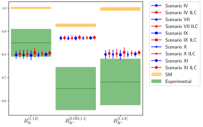
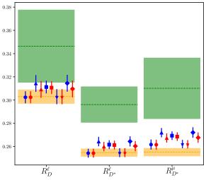
The results for the \RKpand \RDpobservables in the best fit points for the above scenarios are given in FigureΒ 1. We remark that for the \RDpratios, the Cℓ​qΟ„superscriptsubscriptπΆβ„“π‘žπœC_{\ell q}^{\tau} contributions are needed, making scenarios VII, IX and XI preferred over IV and X. Clearly, for a simultaneous analysis of predictions for the \RDpand \RKpobservables, the scenarios with three non-universal Wilson coefficients are favoured.

Refer to caption Refer to caption
Figure 1: Central value and $1\sigma$ uncertainty of the $\RKp$ observables (left), and $\RDp$ observables (right) in scenarios IV, VII, IX, X and XI (blue lines for current predictions, red lines for ILC-based predictions), compared to the SM prediction (yellow) and experimental measurements (green).

Let us stress that new experimental inputs should provide valuable new information to cast light on B anomalies. In this concern, the future $e^{+}e^{-}$ linear collider ILC will offer the opportunity to use the increased precision of the EW observables, thanks to the huge production of $Z$ bosons, to further constrain the global fits. In order to asses the impact of the improved precision on our analysis, we have performed a new global fit inΒ [6], by using for the central values of the EW observables their predictions as in our previous workΒ [5] and taking the uncertainty from the ILC at $\sqrt{s}=$ 250 GeV projections fromΒ [7]. For comparison, the results of the fits to scenarios IV, V and VI; in which two of the Wilson coefficients receive NP contributions simultaneously, both for the current fits at LHC and for the ILC projections, are presented in FigureΒ 2. One can conclude that the LFU-conserving direction of the fit, corresponding to the linear combination $C_{\ell q}^{e}+C_{\ell q}^{\mu}$, is even more tightly constrained due to the better precision of the EW observables. The LFUV direction of the fit remains unchanged, since the EW observables are not sensitive to these deviations.

$\displaystyle-1.00$ $\displaystyle-0.75$ $\displaystyle-0.50$ $\displaystyle-0.25$ $\displaystyle 0.00$ $\displaystyle C_{\ell q}^{e}$ $\displaystyle 0.00$ $\displaystyle 0.25$ $\displaystyle 0.50$ $\displaystyle 0.75$ $\displaystyle 1.00$ $\displaystyle C_{\ell q}^{\mu}$ $\displaystyle R_{K^{(*)}}$ $\displaystyle R_{D^{(*)}}$EW (LHC)EW (ILC)Global (LHC)Global (ILC)
$\displaystyle-0.50$ $\displaystyle-0.25$ $\displaystyle 0.00$ $\displaystyle C_{\ell q}^{e}$ $\displaystyle-1.00$ $\displaystyle-0.75$ $\displaystyle-0.50$ $\displaystyle-0.25$ $\displaystyle 0.00$ $\displaystyle 0.25$ $\displaystyle 0.50$ $\displaystyle 0.75$ $\displaystyle 1.00$ $\displaystyle C_{\ell q}^{\tau}$ $\displaystyle R_{K^{(*)}}$ $\displaystyle R_{D^{(*)}}$EW (LHC)EW (ILC)Global (LHC)Global (ILC)
$\displaystyle-0.50$ $\displaystyle-0.25$ $\displaystyle 0.00$ $\displaystyle 0.25$ $\displaystyle 0.50$ $\displaystyle C_{\ell q}^{\mu}$ $\displaystyle-1.00$ $\displaystyle-0.75$ $\displaystyle-0.50$ $\displaystyle-0.25$ $\displaystyle 0.00$ $\displaystyle 0.25$ $\displaystyle 0.50$ $\displaystyle 0.75$ $\displaystyle 1.00$ $\displaystyle C_{\ell q}^{\tau}$ $\displaystyle R_{K^{(*)}}$ $\displaystyle R_{D^{(*)}}$EW (LHC)EW (ILC)Global (LHC)Global (ILC)
Figure 2: $1\sigma$ and $2\sigma$ contours for several scenarios: Scenario IV (left), Scenario V (center), and Scenario VI (right). Solid lines correspond to the current fits, dash-dotted lines to the fits including the ILC projections.

The results for the central value and $1\sigma$ uncertainty for the \RKpand \RDpobservables in the best fit points for Scenarios IV, VII, IX, X and XI at ILC are also included in FigureΒ 1. The error of the $\RKp$ observables is improved up to factor of 3. When including the ILC projections, the error in all those observables is dominated by the theoretical uncertainty, due to that the allowed region for the Wilson coefficients in the fits is reduced.

Summarising, it is difficult to find an easy common explanation for all flavour anomalies, but the analysis of the effects of the global fit to the Wilson coefficients is mandatory. The anomalies can be described by NP displaying a maximal violation of universality between electrons and muons, but some NP in the tau sector is also needed. It is clear that new experimental inputs and updated global fits to date are needed to clarify the present situation.

References

  • [1] Y.Β S.Β Amhis et al. [HFLAV], Eur.Β Phys.Β J.Β C 81 (2021) 226 [arXiv:1909.12524 [hep-ex]].
  • [2] R.Β Aaij et al. [LHCb], [arXiv:2103.11769 [hep-ex]].
  • [3] R.Β Aaij et al. [LHCb], JHEP 1708 (2017) 055 [arXiv:1705.05802 [hep-ex]].
  • [4] J.Β Alda, J.Β Guasch, S.Β PeΓ±aranda, Eur. Phys. J. C 79 (2019) 588 [arXiv:1805.03636 [hep-ph]]
  • [5] J.Β Alda, J.Β Guasch, S.Β PeΓ±aranda, [arXiv:2012.14799 [hep-ph]].
  • [6] J.Β Alda, J.Β Guasch, S.Β PeΓ±aranda, [arXiv:2105.05095 [hep-ph]].
  • [7] R.Β K.Β Ellis et al., [arXiv:1910.11775 [hep-ex]].