Doubly Robust Stein-Kernelized Monte Carlo Estimator: Simultaneous Bias-Variance Reduction and Supercanonical Convergence

Abstract

Standard Monte Carlo computation is widely known to exhibit a canonical square-root convergence speed in terms of sample size. Two recent techniques, one based on control variate and one on importance sampling, both derived from an integration of reproducing kernels and Stein’s identity, have been proposed to reduce the error in Monte Carlo computation to supercanonical convergence. This paper presents a more general framework to encompass both techniques that is especially beneficial when the sample generator is biased and noise-corrupted. We show our general estimator, which we call the doubly robust Stein-kernelized estimator, outperforms both existing methods in terms of mean squared error rates across different scenarios. We also demonstrate the superior performance of our method via numerical examples.

Keywords: Monte Carlo methods, kernel ridge regression, Stein’s identity, control functionals, importance sampling

1 Introduction

We consider the problem of numerical integration via Monte Carlo simulation. As a generic setup, we aim to estimate the expectation $\theta=\mathbb{E}_{\pi}[f(X)]$ using independent and identically distributed (i.i.d.) samples $x_{i}$, $i\in[n]:=\{1,\cdots,n\}$, drawn from the target distribution $\pi$. A natural Monte Carlo estimator is the sample mean $\hat{\theta}=\frac{1}{n}\sum_{i=1}^{n}f(x_{i})$, which is widely known to be unbiased with mean squared error (MSE) $O(n^{-1})$, a rate commonly referred to as the canonical rate.

In this paper, we are interested in Monte Carlo estimators that are supercanoncial, namely with MSE $o(n^{-1})$. We focus especially on recently proposed Stein-kernelized-based methods. These methods come in two forms, one based on control variate, or more generally control functional (CF), and one based on importance sampling (IS). They are capable of reducing bias or variance of Monte Carlo estimators to the extent that the convergence speed becomes supercanonical. On a high level, these approaches utilize knowledge on the analytical form of the sampling density function (up to a normalizing constant), and apply a “kernelization” of Stein’s identity induced by a reproducing kernel Hilbert space (RKHS) to construct functions or weights that satisfy good properties for CF or IS purpose.

Our main goal in this paper is to study a more general framework to encompass both approaches, by introducing a doubly robust Stein-kernelized (DRSK) estimator. The “doubly robust” terminology borrows from existing approaches in off-policy learning (Dudík et al., 2011, 2014; Jiang and Li, 2016; Farajtabar et al., 2018) where one simultaneously applies control variate and IS to reduce estimation error, and the resulting estimator is no worse than the more elementary estimators. In our setting, we will show that DRSK indeed outperforms kernel-based CF and IS across a range of scenarios, especially when the sample generator is imperfect in that the samples are biased or noise-corrupted. Importantly, distinct from the off-policy learning literature, the superiority of our estimator manifests in terms of faster MSE rates in $n$.

More specifically, we consider a general estimation framework with target quantity $\theta=\mathbb{E}_{\pi}[f(X,Y)]$, where $X$ is a partial list of input variables that is analytically tractable (i.e., its density $\pi_{X}$ known up to a normalizing constant), while $Y$ is a noise term that is not traceable and is embedded in the samples $(x_{i},f(x_{i},y_{i}))$. Moreover, instead of having a generator for $\pi$, we may only have access to a possibly biased generator with distribution $q$. In this setting, we will demonstrate that applying the existing methods of kernel-based CF and IS both encounter challenges. In fact, because of these complications, these estimators could have a subcanonical convergence. On the other hand, our DRSK still exhibits supercanonical rate.

Other than theoretical interest, a motivation of studying our considered general setting pertains to estimation problems that involve epistemic and aleatory variables, which arise when simulation generators are “corrupted”. More concretely, consider a target performance measure that is an expected value of some random outputs (aleatory noise), which are in turn generated from some input models. When the input models themselves are estimated from extrinsic data (epistemic noise), then estimating the target performance measure would involve handling the two sources of noises simultaneously, a common problem in stochastic simulation under input uncertainty (Xie et al., 2014; Zouaoui and Wilson, 2003; Song et al., 2014; Lam, 2016; Corlu et al., 2020; Barton et al., 2022). Here, when the epistemic uncertainty is represented via a Bayesian approach, a natural strategy is to estimate the posterior performance measure, in which $X$ can represent the epistemic uncertainty and $Y$ the aleatory uncertainty. Typically, $X$ follows a posterior distribution that is known up to a normalizing constant, and may need to be generated using variational inference (Wainwright and Jordan, 2008; Blei et al., 2017) or Markov chain Monte Carlo (MCMC) with independent parallel chains (Rosenthal, 2000; Liu and Lee, 2017), so that the realized samples follow a biased distribution $q$ instead of $\pi$ (Liu et al., 2017). Our work primarily focuses on the case where the generated samples of $X$ are independent, while other studies for the case where the samples are not necessarily independent (but without studying supercanonical rates) can be found in, e.g., South et al. (2022b); Belomestny et al. (2021) and references therein. On the other hand, $Y$ could be generated from a black-box simulator that lacks analytical tractability. Such problems with biased epistemic generators and black-box aleatory noises comprise precisely the setup where DRSK is well-suited to enhance the estimation rates.

To be more concrete, below we use a simple generic problem in stochastic simulation to illustrate our problem setting. A more sophisticated example of a computer communication network can be found in Section 4.2 in our numerical experiments.

Example 1

Consider an M/M/1 queue with known arrival rate $1$ and unknown service rate $x$. Since the ground-truth $x$ is unknown, we may estimate $x$ via Bayesian inference based on historical data (say, the actual service time of several customers) and obtain its posterior distribution up to a normalizing constant. By leveraging MCMC or variational inference, only samples from an approximate posterior (instead of the exact posterior) can be drawn. Suppose we are interested in the mean of the waiting time of the first 10 customers. To do this, for each rate $x$, we simulate a fixed number of M/M/1 queues, obtain the waiting time of the first 10 customers in each queue, and output their average $f(x,y)$. Here $y$ represents the intrinsic noise (aleatory uncertainty) in the simulation model since the sample average waiting time given $x$ is still a random proxy for its expectation. The goal is to calculate the expectation of $f(X,Y)$ under the posterior of $X$ and the intrinsic noise of $Y$. Note, moreover, that when using a large or even moderate number of simulated queues, the noise level of $Y$ given $X$ in our estimate is small because of the averaging effect.

Finally, in terms of computational complexity, DRSK costs no more than kernel-based CF and IS. The main computational expense is to solve a kernel ridge regression (KRR) problem (as in kernel-based CF) and a convex quadratic program (as in kernel-based IS), both of which involve a Gram matrix whose dimension is related to the number of the samples. Although computational complexity is not the main focus of this work, we point out that KRR is known to not scale well with the growth of the sample size due to the matrix computation. Hence advanced computational techniques such as divide-and-conquer KRR (Zhang et al., 2013) may be applied when the sample size is large.

In the following, we first introduce some background and review the kernel-based CF and IS (Section 2). With these, we introduce our main DRSK estimator, present its convergence guarantees and compare with the existing methods (Section 3). After that, we demonstrate some numerical experiments to support our method (Section 4). Finally, we develop the theoretical machinery for regularized least-square regression on RKHS needed in our analysis (Section 5) and detail the proofs of our theorems (Section 6).

2 Background and Existing Methods

We first introduce our setting and notations (Section 2.1), then review the technique of kernelization on Stein’s identity in an RKHS (Section 2.2), kernel-based CF (Section 2.3) and IS (Section 2.4), followed by a discussion on other related work (Section 2.5).

2.1 Setting and Notation

Consider a random vector $(X,Y)$ where $X$ takes values in an open set $\Omega\subset\mathbb{R}^{d}$ and $Y$ takes values in an open set $\Gamma\subset\mathbb{R}^{p}$. Our goal is to estimate the expectation of $f(X,Y)$ under a distribution $(X,Y)\sim\pi$, which we denote as $\theta:=\mathbb{E}_{\pi}[f(X,Y)]$. The point estimator will be denoted as $\hat{\theta}$. We assume $X$ admits a positive continuously differentiable marginal density with respect to $d$-dimensional Lebesgue measure, which we denote as $\pi_{X}(x)$. Similarly, we denote $\pi_{Y|X}(y|x)$ as the conditional distribution of $Y$ given $X$ (which is not required to have density).

Our premise is that we can run simulations and have access to a collection of i.i.d. samples $D=\{(x_{i},f(x_{i},y_{i})):i=1,\cdots,n\}$ where $(x_{i},y_{i})$ are drawn from some distribution $q$ (which might be unknown and distinct from $\pi$). It is sometimes useful to think of $X$ as the “dominating” factor in the simulation, contributing the most output variance, whereas $Y$ is an auxiliary noise and contributes a small variance (we will rigorously define these in the theorems later). The small variance from $Y$ can be justified in, e.g., the stochastic simulation setting where typically the modeler simulates and then averages a large number of simulation runs to estimate an expectation-type performance measure; Recall Example 1.

For convenience, for any measurable function $g:\Omega\times\Gamma\to\mathbb{R}$, we write $\mu(g)=\mathbb{E}_{\pi}[g(X,Y)]$, and for any measurable function $g:\Omega\to\mathbb{R}$, we write $\mu_{X}(g)=\mathbb{E}_{\pi_{X}}[g(X)]$. If $g$ is constructed from training data, then $\mu(g)$ and $\mu_{X}(g)$ are understood as the conditional expectation of $g$ given training data. Let $L^{2}(\pi_{X})$ denote the space of measurable functions $g:\Omega\to\mathbb{R}$ for which $\mu_{X}(g^{2})$ is finite, with the norm written as $\|\cdot\|_{L^{2}(\pi_{X})}$. Let $C^{k}(\Omega,\mathbb{R}^{j})$ denote the space of (measurable) functions from $\Omega$ to $\mathbb{R}^{j}$ with continuous partial derivatives up to order $k$. The region $\Omega$ can be bounded or unbounded; in the former case, the boundary $\partial\Omega$ is assumed to be piecewise smooth (i.e., infinitely differentiable).

Similarly, for any measurable function $g:\Omega\times\Gamma\to\mathbb{R}$, we write $\nu(g)=\mathbb{E}_{q}[g(X,Y)]$, and for any measurable function $g:\Omega\to\mathbb{R}$, we write $\nu_{X}(g)=\mathbb{E}_{q_{X}}[g(X)]$. If $g$ is constructed from training data, then $\nu(g)$ and $\nu_{X}(g)$ are understood as the conditional expectation of $g$ given training data. Let $L^{2}(q_{X})$ denote the space of measurable functions $g:\Omega\to\mathbb{R}$ for which $\nu_{X}(g^{2})$ is finite, with the norm written as $\|\cdot\|_{L^{2}(q_{X})}$.

Throughout this paper, we assume that $\pi_{X}\in C^{1}(\Omega,\mathbb{R})$. The score function of the density $\pi_{X}$, $\bm{u}(x):=\nabla_{x}\log\pi_{X}(x)$ is well-defined and is computable for given $x_{i}$’s. This is equivalent to saying $\pi_{X}(x)$ has a parametric form that is known up to a normalizing constant. We also assume that the target function $f:\Omega\times\Gamma\to\mathbb{R}$ satisfies $\mathbb{E}_{\pi}[f(X,Y)^{2}]<\infty$.

2.2 Stein-Kernelized Reproducing Kernel Hilbert Space

We briefly introduce the technique of kernelization on Stein’s identity in an RKHS (Liu et al., 2016; Oates et al., 2017).

We say that a real-valued function $g(x):\Omega\subset\mathbb{R}^{d}\to\mathbb{R}$ is in the Stein class of $\pi_{X}(x)$ (Ley et al., 2017; Liu et al., 2016) if $g(x)$ is continuously differentiable and satisfies

$$\int_{\Omega}\nabla_{x}(\pi_{X}(x)g(x))dx=\bm{0}\in\mathbb{R}^{d}.$$

This condition can be easily checked using integration by parts or the divergence theorem; in particular, it holds if $\pi_{X}(x)g(x)=0$, $\forall x\in\partial\Omega$ when the closure of $\Omega$ is compact, or $\lim_{\|x\|\to\infty}\pi_{X}(x)g(x)=0$ when $\Omega=\mathbb{R}^{d}$. The “canonical” Stein operator of $\pi_{X}$, $\mathcal{A}_{\pi_{X}}$, acting on the Stein class of $\pi_{X}(x)$ is a (linear) operator defined as

$$\mathcal{A}_{\pi_{X}}g(x)=\bm{u}(x)g(x)+\nabla_{x}g(x)\in\mathbb{R}^{d}.$$ (1)

where $\bm{u}(x):=\nabla_{x}\log\pi_{X}(x)$ is the score function of $\pi_{X}(x)$ as introduced earlier. Note that the general definition of the Stein operator typically depends on a class of functions that Stein operator acts on (Gaunt et al., 2019); Yet, if this class of functions is exactly the Stein class of $\pi_{X}(x)$, the “canonical” Stein operator is defined uniquely by (1) as suggested by previous studies (Stein et al., 2004; Liu et al., 2016; Ley et al., 2017; Mijoule et al., 2018).

For any $g(x)$ in the Stein class of $\pi_{X}(x)$, we have the well-known Stein’s identity (Liu et al., 2016; Mijoule et al., 2018) as follows:

$$\mathbb{E}_{\pi_{X}}[\mathcal{A}_{\pi_{X}}g(X)]=\bm{0}$$ (2)

since $\nabla_{x}(\pi_{X}(x)g(x))=\big{(}\bm{u}(x)g(x)+\nabla_{x}g(x)\big{)}\pi_{X}(x)$. In addition, a vector-valued function $\bm{g}(x)=[g_{1}(x),\cdots,g_{d^{\prime}}(x)]$ is said to be in the Stein class of $\pi_{X}(x)$ if every $g_{i}$, $\forall i\in[d^{\prime}]$ is in the Stein class of $\pi_{X}(x)$.

Recall that a Hilbert space $\mathcal{H}$ with an inner product $\langle\cdot,\cdot\rangle:\mathcal{H}\times\mathcal{H}\to\mathbb{R}$ is a RKHS if there exists a symmetric positive definite function $k:\Omega\times\Omega\to\mathbb{R}$, called a (reproducing) kernel, such that for all $x\in\Omega$, we have $k(\cdot,x)\in\mathcal{H}$ and for all $x\in\Omega$ and $h\in\mathcal{H}$, we have $h(x)=\langle h(\cdot),k(\cdot,x)\rangle$. A kernel $k(x,x^{\prime})$ is said to be in the Stein class of $\pi_{X}$ if $k(x,x^{\prime})\in C^{2}(\Omega\times\Omega,\mathbb{R})$, and both $k(x,\cdot)$ and $k(\cdot,x^{\prime})$ are in the Stein class of $\pi_{X}$ for any fixed $x,x^{\prime}$. Note that if $k(x,x^{\prime})$ is in the Stein class of $\pi_{X}$, so is any $h\in\mathcal{H}$ (Liu et al., 2016).

Suppose $k(x,x^{\prime})$ is in the Stein class of $\pi_{X}$. Then it is easy to see that $\nabla_{x^{\prime}}(\pi_{X}(x^{\prime})k(\cdot,x^{\prime}))$ is also in the Stein class of $\pi_{X}$ for any $x^{\prime}$ (Liu et al., 2016):

$$\int_{\Omega}\nabla_{x}\left(\pi_{X}(x)\nabla_{x^{\prime}}(\pi_{X}(x^{\prime})k(x,x^{\prime}))\right)dx=\nabla_{x^{\prime}}\left(\pi_{X}(x^{\prime})\int_{\Omega}\nabla_{x}(\pi_{X}(x)k(x,x^{\prime}))dx\right)=\bm{0}\in\mathbb{R}^{d\times d}$$

since $k(\cdot,x^{\prime})$ is in the Stein class of $\pi_{X}$ for any $x^{\prime}$. Taking the trace of the matrix

$$\text{trace}\left(\nabla_{x}\left(\pi_{X}(x)\nabla_{x^{\prime}}(\pi_{X}(x^{\prime})k(x,x^{\prime}))\right)\right),$$

we get the following kernelized version of Stein’s identity (cf. (2)):

$$\mathbb{E}_{X\sim\pi_{X}}[k_{0}(X,x^{\prime})]=0,\quad\forall x^{\prime}\in\Omega$$ (3)

where $k_{0}(x,x^{\prime})$ is a new kernel function defined via

$$k_{0}(x,x^{\prime}):=\nabla_{x}\cdot\nabla_{x^{\prime}}k(x,x^{\prime})+\bm{u}(x)\cdot\nabla_{x^{\prime}}k(x,x^{\prime})+\bm{u}(x^{\prime})\cdot\nabla_{x}k(x,x^{\prime})+\bm{u}(x)\cdot\bm{u}(x^{\prime})k(x,x^{\prime}).$$

Let $\mathcal{H}_{0}$ be the RKHS related to $k_{0}(x,x^{\prime})$. Then all the functions $h(x)$ in $\mathcal{H}_{0}$ are orthogonal to $\pi_{X}(x)$ in the sense that $\mathbb{E}_{\pi_{X}}[h(X)]=0$ (Liu and Lee, 2017). This proposition is fundamental in the construction of Stein-kernelized CFs. It is easy to check that the commonly used radial basis function (RBF) kernel $k(x,x^{\prime})=\exp(-\frac{1}{h^{2}}\|x-x^{\prime}\|^{2}_{2})$ is in the Stein class for continuously differentiable densities supported on $\mathbb{R}^{d}$.

In addition that the kernel $k$ is in the Stein class, we also assume the gradient-based kernel $k_{0}$ satisfies $\sup_{x\in\Omega}k_{0}(x,x)<\infty.$ In this paper, we always assume $\mathcal{H}_{0}$ satisfies these two conditions. For instance, the RBF kernel $k(x,x^{\prime})=\exp(-\frac{1}{h^{2}}\|x-x^{\prime}\|^{2}_{2})$ satisfies the above two conditions for continuously differentiable densities supported on $\mathbb{R}^{d}$ whose score function $\bm{u}(x)$ is of polynomial growth rate.

Next, let $\mathcal{C}$ denote the RKHS of constant functions with kernel $k_{\mathcal{C}}(x,x^{\prime})=1$ for all $x,x^{\prime}\in\Omega$. The norms associated to $\mathcal{C}$ and $\mathcal{H}_{0}$ are denoted by $\|\cdot\|_{\mathcal{C}}$ and $\|\cdot\|_{\mathcal{H}_{0}}$ respectively. $\mathcal{H}_{+}=\mathcal{C}+\mathcal{H}_{0}$ denotes the set $\{c+\psi:c\in\mathcal{C},\psi\in\mathcal{H}_{0}\}$. Equip $\mathcal{H}_{+}$ with the structure of a vector space, with addition operator $(c+\psi)+(c^{\prime}+\psi^{\prime})=(c+c^{\prime})+(\psi+\psi^{\prime})$ and multiplication operator $\lambda(c+\psi)=(\lambda c)+(\lambda\psi)$, each well-defined due to uniqueness of the representation $f=c+\psi,f^{\prime}=c^{\prime}+\psi^{\prime}$ with $c,c^{\prime}\in\mathcal{C}$ and $\psi,\psi^{\prime}\in\mathcal{H}_{0}$. It is known that $\mathcal{H}_{+}$ can be constructed as an RKHS with kernel $k_{+}(x,x^{\prime}):=k_{\mathcal{C}}(x,x^{\prime})+k_{0}(x,x^{\prime})$ and with norm $\|f\|_{\mathcal{H}_{+}}^{2}:=\|c\|_{\mathcal{C}}^{2}+\|\psi\|_{\mathcal{H}_{0}}^{2}$ (Berlinet and Thomas-Agnan, 2011). Let $\kappa:=\sup_{x\in\Omega}\sqrt{k_{+}(x,x)}$. Note that $\kappa<\infty$ since $\sup_{x\in\Omega}k_{0}(x,x)<\infty$.

Finally, we remark that different choices of the kernel $k$ lead to different constructions of the RKHS $\mathcal{H}_{+}$, and may lead to different performance of subsequent approaches since their performance depends on the regularity of the ground-truth regression function in the space $\mathcal{H}_{+}$. An ideal requirement is that $\mathcal{H}_{+}$ should embody the ground-truth regression function.

2.3 Control Functionals

Control functional (CF), or more precisely Stein-kernelized control functional, first introduced by Oates et al. (2017) and Oates et al. (2019), is a systematically constructed class of control variates for variance reduction (In fact, CF can also partially perform bias reduction as we will show in Section 3). Specifically, CF constructs a function $s_{m}(\cdot)$ applied on $X$ such that $\mu_{X}(s_{m})$ is known, and that $f(X,Y)-s_{m}(X)$ has a very low variance so that the CF-adjusted sample

$$f(X,Y)-s_{m}(X)+\mathbb{\mu}_{X}(s_{m})$$

is supercanonical for estimating $\mathbb{E}_{\pi}[f(X,Y)]$. This function $s_{m}(\cdot)$ is constructed as a functional approximation for $f(\cdot)$ by utilizing a training set of samples, where the function lies in the RKHS $\mathcal{H}_{+}$ constructed in Section 2.2 which has known mean under the distribution $\pi$.

In more detail, following Oates et al. (2017), we divide the data $D$ into two disjoint subsets as $D_{0}=\{(x_{i},y_{i})\}^{m}_{i=1}$ and $D_{1}=\{(x_{i},y_{i})\}^{n}_{i=m+1}$, where $1\leq m<n$. $D_{0}$ is used to construct a function $s_{m}(\cdot)\in L^{2}(\pi_{X})$ that is a partial approximation to $f$ (that only depends on $x$). $s_{m}(x)$ is given by the following regularized least-square (RLS) functional regression on the RKHS $\mathcal{H}_{+}$, also known as kernel ridge regression (KRR):

$$s_{m}(x):=\mathop{\arg\min}_{g\in\mathcal{H}_{+}}\left\{\frac{1}{m}\sum_{j=1}^{m}(f(x_{j},y_{j})-g(x_{j}))^{2}+\lambda\|g\|^{2}_{\mathcal{H}_{+}}\right\}$$

where $\lambda>0$ is a regularization parameter which typically depends on the cardinality of the data set $D_{0}$. Note that in CF, the RKHS space $\mathcal{H}_{+}$ instead of $\mathcal{H}_{0}$ is the hypothesis class used in the KRR because $\mathcal{H}_{0}$ only contains functions with mean zero that cannot effectively approximate the function $f$ with a general mean. Consider the function

$$f_{m}(x,y)=f(x,y)-s_{m}(x)+\mu_{X}(s_{m}).$$ (4)

Then the CF estimator is given by a sample average of $f_{m}(\cdot,\cdot)$ on $D_{1}$, i.e.,

$$\hat{\theta}_{CF}:=\frac{1}{n-m}\sum_{j=m+1}^{n}f_{m}(x_{j},y_{j}).$$

If $(x_{i},y_{i})$ are i.i.d. drawn from the original distribution $\pi$, it is clear that we have unbiasedness, since $\mathbb{E}_{\pi}[\hat{\theta}_{CF}|D_{0}]=\mu(f_{m})=\theta$ for any given $D_{0}$ and hence $\mathbb{E}_{\pi}[\hat{\theta}_{CF}]=\theta$. On the other hand, suppose our data $D$ are drawn from a distribution $q$ which may be different from the original distribution $\pi$. Then given $D_{0}$ (and thus given $s_{m}$), one component $f_{m}(X,Y)$ is in general biased for $\theta$ and the resulting CF by taking their average can suffer as a result.

It is well known in the KRR literature that the $s_{m}$ can be written explicitly in a closed form. We will review this result in Section 6.1 and in particular, rewrite the existing closed-form solution from Oates et al. (2017) in terms of $k_{+}$ rather than $k_{0}$. In summary, CF is described in Algorithm 1. In addition, Oates et al. (2017) suggested a simplified version of CF, called the simplified CF estimator, which is simply the $\mu_{X}(s_{n})$ by setting $m=n$ in Algorithm 1. This estimator is described in Algorithm 2 for the sake of completeness.

Goal: Estimate $\theta:=\mathbb{E}_{\pi}[f(X,Y)]$;

Input: A set of i.i.d. samples $D=\{(x_{j},z_{j}=f(x_{j},y_{j}))\}_{j=1,\cdots,n}$ drawn from some distribution $q$, the reproducing kernel $k_{0}$ of $\mathcal{H}_{0}$ and $k_{+}=k_{0}+1$ of $\mathcal{H}_{+}$;

Procedure: (1) We divide the dataset $D$ into two disjoint subsets as $D_{0}=\{(x_{i},f(x_{i},y_{i}))\}^{m}_{i=1}$ and $D_{1}=\{(x_{i},f(x_{i},y_{i}))\}^{n}_{i=m+1}$, where $1\leq m<n$;

(2) $D_{0}$ is used to construct the CF-adjusted sample

$$f_{m}(x,y)=f(x,y)-s_{m}(x)+\mu_{X}(s_{m}).$$

Let

$$\hat{z}=(f(x_{1},y_{1}),\cdots,f(x_{m},y_{m}))^{T},$$

$$K_{+}=(k_{+}(x_{i},x_{j}))_{i,j=1,\cdots,m},$$

$$\hat{k}_{+}(x)=(k_{+}(x_{1},x),\cdots,k_{+}(x_{m},x))^{T},$$

$$\beta=(K_{+}+\lambda mI)^{-1}\hat{z}.$$

Then $s_{m}(x)=\beta^{T}\hat{k}_{+}(x)$ and $\mu_{X}(s_{m})=\beta^{T}\mathbf{1}$.

Output: CF estimator

$$\hat{\theta}_{CF}:=\sum_{j=m+1}^{n}\frac{1}{n-m}f_{m}(x_{j},y_{j}).$$

Algorithm 1 Stein-Kernelized Control Functional (CF)

Goal: Estimate $\theta:=\mathbb{E}_{\pi}[f(X,Y)]$;

Input: A set of i.i.d. samples $D=\{(x_{j},z_{j}=f(x_{j},y_{j}))\}_{j=1,\cdots,n}$ drawn from some distribution $q$, the reproducing kernel $k_{0}$ of $\mathcal{H}_{0}$ and $k_{+}=k_{0}+1$ of $\mathcal{H}_{+}$;

Procedure: Let

$$\hat{z}=(f(x_{1},y_{1}),\cdots,f(x_{n},y_{n}))^{T},$$

$$K_{+}=(k_{+}(x_{i},x_{j}))_{i,j=1,\cdots,n},$$

$$\hat{k}_{+}(x)=(k_{+}(x_{1},x),\cdots,k_{+}(x_{n},x))^{T},$$

$$\beta=(K_{+}+\lambda nI)^{-1}\hat{z}.$$

Then $\mu_{X}(s_{n})=\beta^{T}\mathbf{1}$.

Output: Simplified CF estimator

$$\hat{\theta}_{SimCF}:=\mu_{X}(s_{n}).$$

Algorithm 2 Simplified CF Estimator (SimCF)

2.4 Black-Box Importance Sampling

Another method derived from the kernelization of Stein’s identity is black-box importance sampling (BBIS) introduced by Liu and Lee (2017), which has been shown to be an effective approach for both variance and bias reduction. This method can be viewed as a relaxation of conventional IS, in that it assigns weights over the samples assuming that the data are drawn from a sampling distribution $q$ in the black box, i.e., with no knowledge on the analytical form of $q$. In this setting, standard importance weights cannot be calculated because the likelihood ratio is unknown. In the situation where the noise $Y$ does not appear, the black-box importance weights are optimized based on a convex quadratic minimization problem:

$$\mathop{\arg\min}_{w}\{w^{T}K_{0}w:w\geq 0,w^{T}\textbf{1}=1\}$$ (5)

where $\textbf{1}=(1,1,\cdots,1)$ and $K_{0}$ is the kernel matrix with respect to the RKHS $\mathcal{H}_{0}$ constructed in Section 2.2 which contains functions with mean zero under the distribution $\pi_{X}$. Suppose $w$ is the (unknown) likelihood ratio between $\pi_{X}$ and $q_{X}$, i.e., $w_{i}=\frac{1}{n}\frac{\pi_{X}(x_{i})}{q_{X}(x_{i})}$. Then

$$\mathbb{E}_{x_{i}\sim q_{X}}[w_{i}k_{0}(x_{i},x_{j})w_{j}]=\frac{1}{n}\mathbb{E}_{x_{i}\sim\pi_{X}}[k_{0}(x_{i},x_{j})w_{j}]=0$$

for any $x_{j}$ since the kernel function has mean zero under $\pi_{X}$; see (3). In addition, we have $\mathbb{E}_{q_{X}}[w^{T}\textbf{1}]=1$. Therefore the quadratic form achieves the minimum mean $0$ under $q_{X}$ when $w$ is the likelihood ratio, which intuitively justifies (5).

We provide more details in the general situation. First, we define the empirical kernelized Stein discrepancy (KSD) between the weighted empirical distribution of the samples and $\pi_{X}$:

$$\mathbb{S}(\{x_{j},w_{j}\},\pi_{X})=\sum_{j,k\in D}w_{j}w_{k}k_{0}(x_{j},x_{k})=w^{T}K_{0}w.$$

where

$$K_{0}=(k_{0}(x_{j},x_{k}))_{j,k\in D}$$

is the $n\times n$ kernel matrix constructed on the entire data set $D$. The black-box importance weights then form the optimal solution to the following convex quadratic optimization problem (which can be solved efficiently):

$$\hat{w}=\mathop{\arg\min}_{w}\left\{\mathbb{S}(\{x_{j},w_{j}\},\pi_{X}),\text{ s.t. }\sum_{j=1}^{n}w_{j}=1,0\leq w_{j}\leq\frac{B_{0}}{n}\right\}$$ (6)

where $B_{0}$ is a pre-specified bound that will be provided in the subsequent theorems. Here, the upper bound $B_{0}$ on the weights is a new addition compared to the original formulation in Liu and Lee (2017), and is needed to control the MSE when there is the noise term $Y$. The BBIS estimator is given by a weighted average of $f(\cdot,\cdot)$ on $D$, i.e.,

$$\hat{\theta}_{IS}:=\sum_{j=1}^{n}\hat{w}_{j}f(x_{j},y_{j}).$$

In summary, BBIS is described in Algorithm 3.

Goal: Estimate $\theta:=\mathbb{E}_{\pi}[f(X,Y)]$;

Input: A set of i.i.d. samples $D=\{(x_{j},z_{j}=f(x_{j},y_{j}))\}_{j=1,\cdots,n}$ drawn from some distribution $q$, the reproducing kernel $k_{0}$ of $\mathcal{H}_{0}$;

Procedure: Let

$$K_{0}=(k_{0}(x_{i},x_{j}))_{i,j=1,\cdots,n},$$

and $\hat{w}$ is the optimal solution to the following quadratic optimization problem

$$\hat{w}=\mathop{\arg\min}_{w}\left\{w^{T}K_{0}w,\text{ s.t. }\sum_{j=1}^{n}w_{j}=1,0\leq w_{j}\leq\frac{B_{0}}{n}\right\}.$$ (7)

If the noise $Y$ does not exist, we simply set $B_{0}=+\infty$. Otherwise, set $B_{0}=2B$ for the canonical rate and $B_{0}=4B$ for a supercanonical rate (see Assumption 4 for the definition of $B$ and Theorem 8 for details).

Output: BBIS estimator

$$\hat{\theta}_{IS}:=\sum_{j=1}^{n}\hat{w}_{j}f(x_{j},y_{j}).$$

Algorithm 3 Modified Black-Box Importance Sampling (BBIS)

2.5 Related Work

To close this section, we discuss some other related literature. Variance and bias reduction has been a long-standing topic in Monte Carlo simulation. Two widely used methods are control variates and importance sampling (Chapter 4 in Glasserman (2003), Chapter 5 in Asmussen and Glynn (2007), Chapter 5 in Rubinstein and Kroese (2016)). The control variate method reduces variance by adding an auxiliary variate with known mean to the naive Monte Carlo estimator (Nelson, 1990). The construction of this auxiliary variable can follow multiple approaches. In the classical setup, a fixed number of control variates are linearly combined, with the linear coefficients constructed by ordinary least squares (Glynn and Szechtman, 2002). This approach maintains the canonical rate in general. Beyond this, one can add a growing number of control variates (relative to the sample size) to get a faster rate (Portier and Segers, 2018). The linear coefficients can also be obtained by using regularized least squares to increase accuracy (South et al., 2022a; Leluc et al., 2021). These methods require a pre-specified collection of well-behaved control variates (e.g., the control variates are linearly independent or dense in a function space), which may not always be easy to construct in practice.

To generalize the linear form and possibly obtain a supercanonical rate, the control variate can be constructed via a fitted function learned from data. This function can be constructed using adaptive control variates (Henderson and Glynn, 2002; Henderson and Simon, 2004; Kim and Henderson, 2007). In order to have a supercanonical rate for adaptive control variate estimators, one of the key assumptions in these papers is the existence of a “perfect” control variate (i.e., a control variate with zero variance), and the “perfect” control variate can be approximated in an adaptive scheme. This assumption could be unlikely to hold for some practical applications (Kim and Henderson, 2007). Another approach to construct the function is via $L^{2}$ functional approximation (Maire, 2003). Maire (2003) only focuses on the mono-dimensional function whose $L^{2}$ expansion coefficients decrease at a polynomial rate. It is unknown how to extend this work to multi-dimensional functions. Finally, the function can also be constructed, as described earlier, via RLS regression (Oates et al., 2017) which provides a systematic approach to construct control variates based on the kernelization of Stein’s identity. Compared with previous methods, Oates et al. (2017) require less restrictive assumptions for supercanonical rates and avoid adaptive tuning procedures.

Standard IS reduces variance by using an alternate proposal distribution to generate samples, and multiplying the samples by importance weights constructed from the likelihood ratios, or the Radon-Nikodym derivative, between the proposal and original distributions. Likewise, it can also be used to de-bias estimates through multiplying by likelihood ratios if the generating distribution is biased. IS has been shown to be powerful in increasing the efficiency of rare-event simulation (Bucklew, 2013; Rubino and Tuffin, 2009; Juneja and Shahabuddin, 2006; Blanchet and Lam, 2012). In contrast to conventional methods, BBIS does not require the closed form of the likelihood ratio. We also note that both CF and BBIS can be viewed as versions of the weighted Monte Carlo method since both of them can be written in the form of a linear combination of $f(x_{i})$, while their weights are obtained in different ways. Other methods to construct weighted Monte Carlo can be found in, e.g., Glasserman and Yu (2005); Owen and Zhou (2000).

Besides the Monte Carlo literature, CF utilizes a combination of two ideas: kernel ridge regression (KRR) and the Stein operator. The theory of KRR has been well developed in the past two decades. Its modern learning theory has been proposed in Cucker and Smale (2002a) and Cucker and Smale (2002b), and further strengthened in Smale and Zhou (2004), Smale and Zhou (2005) and Smale and Zhou (2007). Cucker and Zhou (2007) provide comprehensive documentation on this topic. Most of these works assume that the input space is a compact set. Sun and Wu (2009) further study KRR on non-compact metric spaces, which provides the mathematical foundation of this paper. There are multiple studies on extending the standard KRR. For instance, Sun and Wu (2010) study KRR with dependent samples. Christmann and Steinwart (2007); Debruyne et al. (2008) study consistency and robustness of kernel-based regression. To relieve the computation cost of KRR estimators for large datasets, Rahimi and Recht (2008) propose the random Fourier feature sampling to speed up the evaluation of the kernel matrix, and Zhang et al. (2013) propose a divide-and-conquer KRR to decompose the computation.

The second idea used by CF is the kernelization of Stein’s identity, i.e., applying the Stein operator to a “primary” RKHS. The resulting RKHS automatically satisfies the zero-mean property under $\pi$ which lays the foundation for constructing suitable control variates. This idea has been used and followed up in Oates et al. (2017, 2019); Lam and Zhang (2019); South et al. (2022b), and finds usage beyond control variates, including the Stein variational gradient descent (Liu and Wang, 2016; Liu, 2017; Liu et al., 2017; Han and Liu, 2018; Wang and Liu, 2019), the kernel test for goodness-of-fit (Chwialkowski et al., 2016; Liu et al., 2016) and BBIS (Liu and Lee, 2017; Hodgkinson et al., 2020) that we have described earlier.

3 Doubly Robust Stein-Kernelized Estimator

We propose an enhancement of CF and BBIS that can simultaneously perform both variance and bias reduction. We call it the doubly robust Stein-kernelized (DRSK) estimator. In brief, we divide the data $D$ into two disjoint subsets as $D_{0}=\{(x_{i},y_{i})\}^{m}_{i=1}$ and $D_{1}=\{(x_{i},y_{i})\}^{n}_{i=m+1}$, where $1\leq m<n$. Based on the first subset $D_{0}$, we construct the same regression function $s_{m}(\cdot)\in L^{2}(\pi_{X})$ to derive the CF-adjusted sample $f_{m}(x,y)$ as in Section 2.3 for variance reduction. Based on the second subset $D_{1}$, we generate the black-box importance weights $\hat{w}$ as in Section 2.4 for bias reduction. Finally, we take the weighted average of $f_{m}(x_{j},y_{j})$ with weights $\hat{w}$ on $D_{1}$ to get the DRSK estimator. The detailed procedure is described in Algorithm 4.

The terminology “doubly robust” in DRSK is borrowed from doubly robust estimators in off-policy learning (Dudík et al., 2011, 2014; Jiang and Li, 2016; Farajtabar et al., 2018). In fact, we can rewrite the DRSK estimator as

$$\hat{\theta}_{DRSK}:= \sum_{j=m+1}^{n}\hat{w}_{j}f_{m}(x_{j},y_{j})$$

$$= \sum_{j=m+1}^{n}\hat{w}_{j}(f(x_{j},y_{j})-s_{m}(x_{j})+\mu_{X}(s_{m}))$$

$$= \mu_{X}(s_{m})+\sum_{j=m+1}^{n}\hat{w}_{j}(f(x_{j},y_{j})-s_{m}(x_{j}))$$ (8)

The doubly robust estimator (Dudík et al., 2014) is known to be a combination of two approaches: direct method (DM) and inverse propensity score (IPS). The second term in (8) is an importance-sampling weighted average of the residuals from the regression, which is similar to the part of IPS in doubly robust estimators. The first term in (8) is similar to the DM by using $s_{m}$ as an approximation of $f$:

$$\sum_{j=m+1}^{n}\frac{1}{n-m}s_{m}(x_{j})$$

except that in our setting, there is no need to estimate the expectation of $s_{m}$ under $\pi$ since $s_{m}\in\mathcal{H}_{+}$ has a known expectation by our construction. Note that the first term in (8) is essentially the simplified CF estimator suggested by Oates et al. (2017) (Algorithm 2). In this sense, CF is similar to DM.

Goal: Estimate $\theta:=\mathbb{E}_{\pi}[f(X,Y)]$;

Input: A set of i.i.d. samples $D=\{(x_{j},z_{j}=f(x_{j},y_{j}))\}_{j=1,\cdots,n}$ drawn from some distribution $q$, the reproducing kernel $k_{0}$ of $\mathcal{H}_{0}$ and $k_{+}=k_{0}+1$ of $\mathcal{H}_{+}$;

Procedure: (1) We divide the dataset $D$ into two disjoint subsets as $D_{0}=\{(x_{i},f(x_{i},y_{i}))\}^{m}_{i=1}$ and $D_{1}=\{(x_{i},f(x_{i},y_{i}))\}^{n}_{i=m+1}$, where $1\leq m<n$;

(2) $D_{0}$ is used to construct the CF-adjusted sample

$$f_{m}(x,y)=f(x,y)-s_{m}(x)+\mu_{X}(s_{m}).$$

Let

$$\hat{z}=(f(x_{1},y_{1}),\cdots,f(x_{m},y_{m}))^{T},$$

$$K_{+}=(k_{+}(x_{i},x_{j}))_{i,j=1,\cdots,m},$$

$$\hat{k}_{+}(x)=(k_{+}(x_{1},x),\cdots,k_{+}(x_{m},x))^{T},$$

$$\beta=(K_{+}+\lambda mI)^{-1}\hat{z}.$$

Then $s_{m}(x)=\beta^{T}\hat{k}_{+}(x)$ and $\mu_{X}(s_{m})=\beta^{T}\mathbf{1}$. (See Section 6.1 for details.)

(3) $D_{1}$ is used to construct the importance weights $\hat{w}$. Let

$$K_{0}=(k_{0}(x_{i},x_{j}))_{i,j=m+1,\cdots,n},$$

and $\hat{w}$ is the optimal solution to the following quadratic optimization problem

$$\hat{w}=\mathop{\arg\min}_{w}\left\{w^{T}K_{0}w,\text{ s.t. }\sum_{j=m+1}^{n}w_{j}=1,0\leq w_{j}\leq\frac{B_{0}}{n-m}\right\}$$ (9)

If the noise $Y$ does not exist, we simply set $B_{0}=+\infty$. Otherwise, set $B_{0}=2B$ for the canonical rate and $B_{0}=4B$ for a supercanonical rate (see Assumption 4 for the definition of $B$ and Theorems 1 and 2 for details).

Output: DRSK estimator

$$\hat{\theta}_{DRSK}:=\sum_{j=m+1}^{n}\hat{w}_{j}f_{m}(x_{j},y_{j}).$$

Algorithm 4 Doubly Robust Stein-Kernelized Estimator (DRSK)

3.1 Main Findings and Comparisons

We summarize our main findings and comparisons of DRSK with the existing CF and BBIS methods. To facilitate our comparisons, recall that in Section 2.1 we have proposed a general problem setting where input samples are both partially known (meaning we have a noise term $Y$) and biased (meaning $(X,Y)$ may not be drawn from the original distribution $\pi$). Here, we elaborate and consider the following four scenarios in roughly increasing level of complexity, where the last case corresponds to the general setting introduced earlier:
(1) “Standard”: there is no noise term $Y$ and $X$ is drawn from $\pi$.
(2) “Partial”: there is a noise term $Y$ and $(X,Y)$ is drawn from $\pi$.
(3) “Biased”: there is no noise term $Y$ and $X$ is drawn from $q$.
(4) “Both”: there is a noise term $Y$ and $(X,Y)$ is drawn from $q$.

We will frequently use the abbreviations “Standard”, “Partial”, “Biased”, “Both” to refer to each case. Tables 1 summarizes the MSE rates of three different methods in each scenario with some common assumptions specified in Section 3.2. In particular, the ground-truth regression function $\bar{f}:=\mathbb{E}_{\pi}[f(X,Y)|X=x]\in\text{Range}(L_{q}^{r})$ with $\frac{1}{2}\leq r\leq 1$ indicating the regularity of $\bar{f}$ in the space $\mathcal{H}_{+}$ where the positive self-adjoint operator $L_{q}$ is formally defined later in (10). $M_{0}$ is given in Assumptions 2 that is the bound on the noise level of $Y$ given $X$.

Table 1: This table displays the MSE rates of three different methods in each scenario with some common assumptions specified in Section 3.2. The ground-truth regression function $\bar{f}:=\mathbb{E}_{\pi}[f(X,Y)|X=x]\in\text{Range}(L_{q}^{r})$ with $\frac{1}{2}\leq r\leq 1$. $M_{0}$ is given in Assumptions 2.

MSE	Standard	Partial	Biased	Both
CF (Ass. 1, 2, 3)	$O(n^{-1-r})$	$O(n^{-1-r})+M_{0}n^{-1}$	$O(n^{-r})$	$O(n^{-r})+M_{0}$
BBIS (Ass. 1, 2, 4)	$O(n^{-1})$	$O(n^{-1})$	$O(n^{-1})$	$O(n^{-1})$
BBIS (Ass. 1, 2, 4, 5)	$o(n^{-1})$	$o(n^{-1})+M_{0}n^{-1}$	$o(n^{-1})$	$o(n^{-1})+M_{0}n^{-1}$
DRSK (Ass. 1, 2, 4)	$O(n^{-\frac{1}{2}-r})$	$O(n^{-\frac{1}{2}-r})+M_{0}n^{-1}$	$O(n^{-\frac{1}{2}-r})$	$O(n^{-\frac{1}{2}-r})+M_{0}n^{-1}$
DRSK (Ass. 1, 2, 4, 5)	$o(n^{-\frac{1}{2}-r})$	$o(n^{-\frac{1}{2}-r})+M_{0}n^{-1}$	$o(n^{-\frac{1}{2}-r})$	$o(n^{-\frac{1}{2}-r})+M_{0}n^{-1}$

Table 1 conveys the following:

1. Except that the noise part remains at the canonical rate, CF has a supercanonical rate in the “Standard” and “Partial” cases, but subcanonical in the “Biased” and “Both” cases when $r<1$. In the following, the supercanonical and subcanonical rates are referred to as the property on the “dominating” factor $X$ with the convention that the noise $Y$ is at the canonical rate.

2. BBIS in all cases has the canonical rate under a weak assumption and a supercanonical rate under a strong assumption (Assumption 5).

3. DRSK always has a supercanonical rate either when $r>\frac{1}{2}$ or under a strong assumption (Assumption 5).

4. Suppose $r>\frac{1}{2}$. Then DRSK is strictly faster than CF and BBIS in the “Biased” and “Both” cases, under both weak and strong assumptions. Moreover, DRSK is strictly faster than BBIS in any case, under both weak and strong assumptions.

CF can handle extra noise quite well (in the “Standard” and “Partial” cases) since it takes advantage of the functional approximation of $f$, but only partially reduce bias. In the “Biased” and “Both” cases, a single component $f_{m}(X,Y)$ (with finite $m$) in CF is generally a biased estimator of $\theta$. The uniform weight $\frac{1}{n-m}$ in the final step of constructing CF cannot reduce the bias in $f_{m}-\theta$ effectively, which leads to underperformance in the “Biased” and “Both” cases. Therefore, the simplified CF estimator (Algorithm 2) could be a better alternative by omitting the final step, as recommended by Oates et al. (2017). On the other hand, our results also show that a single $f_{m}(X,Y)$ is an asymptotically unbiased estimator of $\theta$ (at the rate of $O(m^{-r})$ when $m\to\infty$), indicating the bias reduction perspective of CF.

BBIS performs efficiently for bias reduction in general, although no higher order than $o(n^{-1})$ is guaranteed theoretically. The validity of reducing the MSE in the BBIS estimator is entirely due to the black-box importance weights, ignoring the information of the function $f$ and the output data $f(x_{i},y_{i})$. This implies that a more “regular” function $f$ in the RKHS may not be able to improve the rate in BBIS as CF does. Besides, the original BBIS estimator faces an additional challenge of not controlling the noise term (though the latter is not shown in Table 1).

Therefore, CF and BBIS both encounter difficulties when applying in the “Both” case. Our DRSK estimator improves CF and BBIS by taking advantage of both estimators. The weighting part in DRSK utilizes knowledge of $\pi_{X}$ to diminish the bias as in BBIS, and the control functional part in DRSK utilizes the information of $f(x_{j},y_{j})$ to learn a more “concentrated” function than $f(x)$ as in CF. As shown in Table 1, it can reduce the overall variance and bias efficiently.

3.2 Assumptions

To present our main theorems rigorously, we will employ the following assumptions.

Assumption 1 (Covariate shift assumption)

$\pi_{Y|X}(y|x)=q_{Y|X}(y|x)$.

Here we do not require $\pi_{Y|X}(y|x)$ to be known or to be a continuous probability distribution. Covariate shift assumption holds, for instance, 1) when $X$ is independent of $Y$, or 2) in stochastic simulation problems where the aleatory noise in the simulation output $Y$, conditional on the input parameter $X$, is not affected by the epistemic noise incurred by the input parameter estimation (e.g., $X$ is estimated via historical data independent of the simulation model). Example 1 in Section 1 and the computer communication network in Section 4.2 provide concrete examples where covariate shift assumption holds. Though not directly relevant to our work, we note that the assumption is standard in transfer learning or covariate shift problems (Gretton et al., 2009; Yu and Szepesvári, 2012; Kpotufe and Martinet, 2021; Li et al., 2020). We remark that under this assumption, the ground-truth regression function $f_{\pi}(x):=\mathbb{E}_{\pi}[f(X,Y)|X=x]$ and $f_{q}(x):=\mathbb{E}_{q}[f(X,Y)|X=x]$ are the same so we denote it as $\bar{f}$. We will use crucially the decomposition

$$f(X,Y)=\bar{f}(X)+\epsilon(X,Y)$$

where $\bar{f}(X)$ can be viewed as the contribution of the fluctuation on $f$ from $X$, and $\epsilon(X,Y)=f(X,Y)-\bar{f}(X)$ is the error term. Note that, by definition, we have

$$\mathbb{E}[\epsilon(X,Y)]=0,\quad\mathbb{E}[\epsilon(X,Y)|X]=0,\quad\mathbb{E}[\epsilon(X,Y)\bar{f}(X)]=0$$

where the expectation can be taken with respect to $\pi$ or $q$ under Assumption 1. Next, we introduce a basic assumption on the error term.

Assumption 2

$\mathbb{E}_{q}[\epsilon(X,Y)^{2}]\leq M_{0}<\infty$.

The following assumptions are considered in Liu and Lee (2017) for the biased input samples.

Assumption 3

$\mathbb{E}_{x\sim q_{X}}[(\frac{\pi_{X}(x)}{q_{X}(x)})^{2}]=\mathbb{E}_{x\sim\pi_{X}}[\frac{\pi_{X}(x)}{q_{X}(x)}]<\infty$.

Assumption 4

$\frac{\pi_{X}(x)}{q_{X}(x)}\leq B<\infty\quad\forall x\in\Omega$.

Note that this assumption implies that

$$\mathbb{E}_{x\sim q_{X}}\left[(\frac{\pi_{X}(x)}{q_{X}(x)})^{2}k_{0}(x,x)\right]<\infty,$$

$$\mathbb{E}_{x,x^{\prime}\sim q_{X}}\left[\left(\frac{\pi_{X}(x)}{q_{X}(x)}\frac{\pi_{X}(x^{\prime})}{q_{X}(x^{\prime})}k_{0}(x,x^{\prime})\right)^{2}\right]<\infty.$$

The reason is that we assume $\sup_{x\in\Omega}k_{0}(x,x)<\infty$ in our construction of $\mathcal{H}_{0}$ and we note the fact that $|k_{0}(x,x^{\prime})|\leq(k_{0}(x,x)k_{0}(x^{\prime},x^{\prime}))^{\frac{1}{2}}.$ Therefore, Assumption 3 is the same as Assumption B.1 in Liu and Lee (2017). Moreover, Assumption 4 implies Assumption 3.

Assumption 5

Suppose $k_{0}(x,x^{\prime})$ has the following eigen-decomposition

$$k_{0}(x,x^{\prime})=\sum_{l=1}^{\infty}\lambda_{l}\phi_{l}(x)\phi_{l}(x^{\prime}),$$

where $\{\lambda_{l}\}_{l=1}^{\infty}$ are the positive eigenvalues sorted in non-increasing order, and $\{\phi_{l}\}_{l=1}^{\infty}$ are the eigenfunctions orthonormal w.r.t. the distribution $\pi_{X}(x)$, i.e., $\mathbb{E}_{x\sim\pi_{X}}[\phi_{l}(x)\phi_{l^{\prime}}(x)]=\textbf{1}_{l=l^{\prime}}$. We assume that $\operatorname{trace}(k_{0}(x,x^{\prime}))=\sum_{l=1}^{\infty}\lambda_{l}<\infty$ and $\sup_{x\in\Omega,l}|\phi_{l}(x)|<\infty$.

Assumption 4 plus Assumption 5 is the same as Assumption B.4 in Liu and Lee (2017). In particular, we notice that

$$\text{var}_{x\sim q_{X}}\Big{[}(\frac{\pi_{X}(x)}{q_{X}(x)})^{2}\phi_{l}(x)\phi_{l^{\prime}}(x)\Big{]}\leq\Big{(}\sup_{x\in\Omega}\frac{\pi_{X}(x)}{q_{X}(x)}\Big{)}^{4}\Big{(}\sup_{x\in\Omega,l}|\phi_{l}(x)|\Big{)}^{4}.$$

To simplify notations, we denote $M_{2}$ as the upper bounds in Assumptions 4 and 5, i.e.,

$$\sup_{x\in\Omega}\frac{\pi_{X}(x)}{q_{X}(x)}\leq M_{2},\quad\sup_{x\in\Omega,l}|\phi_{l}(x)|\leq M_{2},\quad\text{var}_{x\sim q_{X}}\Big{[}(\frac{\pi_{X}(x)}{q_{X}(x)})^{2}\phi_{l}(x)\phi_{l^{\prime}}(x)\Big{]}\leq M_{2}$$

where the single value $M_{2}$ is introduced only for the convenience of our proof.

Finally, the integral operator $L_{q}:L^{2}(q_{X})\to L^{2}(q_{X})$ is defined as follows:

$$(L_{q}g)(x):=\int_{\Omega}k_{+}(x,x^{\prime})g(x^{\prime})q_{X}(x^{\prime})dx^{\prime},\ x\in\Omega,\ g\in L^{2}(q_{X}).$$ (10)

This operator can be viewed as a positive self-adjoint operator on $L^{2}(q_{X})$. We can define $L_{\pi}:L^{2}(\pi_{X})\to L^{2}(\pi_{X})$ in a similar way. Note that the power function of $L_{q}$, $L_{q}^{r}$, is well-defined as a positive self-adjoint operator as $L_{q}$ is a positive self-adjoint operator. Denote $\text{Range}(L_{q}^{r})$ the range of $L_{q}^{r}$ on the domain $L^{2}(q_{X})$. Note that a larger $r\geq\frac{1}{2}$ in $\text{Range}(L_{q}^{r})$ corresponds to a more regular (and smaller) subspace of $L^{2}(q_{X})$: $\text{Range}(L_{q}^{r_{1}})\subset\text{Range}(L_{q}^{r_{2}})$ whenever $r_{1}\geq r_{2}$. Conventionally, we write $L_{q}^{-r}g\in L^{2}(q_{X})$ if (1) $g\in\text{Range}(L_{q}^{r})$, (2) $L_{q}^{-r}g$ is an element in the preimage set of $g$ under the operator $L_{q}^{r}$ on the domain $L^{2}(q_{X})$. Further details about the operator $L_{q}^{r}$ can be found in Section 5.

3.3 Convergence of Doubly Robust Stein-Kernelized Estimator

We are now ready to present the main theorems for our DRSK estimator (Algorithm 4). All the theorems are understood in the following way: If the noise term $Y$ does not exist, then we drop Assumptions 1-2 (since they are automatically true) and set $M_{0}=0$ in the results; If $\pi=q$, then we drop Assumptions 3-4 (since they are automatically true) with $B=1$.

Theorem 1 (DRSK in all cases under weak assumptions)

Suppose Assumptions 1, 2, and 4 hold. Take an RLS estimate with $\lambda=m^{-\frac{1}{2}}$ and $B_{0}=2B$ in (9). Let $m=\alpha n$ where $0<\alpha<1$. If $\bar{f}\in\text{Range}(L_{q}^{r})$ ($\frac{1}{2}\leq r\leq 1$), then $\mathbb{E}_{q}[(\hat{\theta}_{DRSK}-\theta)^{2}]\leq C_{1}(C_{f}n^{-\frac{1}{2}-r}+M_{0}n^{-1})$ where $C_{f}=\|L_{q}^{-r}\bar{f}\|^{2}_{L^{2}(q_{X})}$ (which is a constant indicating the regularity of $\bar{f}$ in $\mathcal{H}_{+}$), $C_{1}$ only depends on $\alpha,\kappa,B$.

Next we can obtain a better result with a stronger assumption.

Theorem 2 (DRSK in all cases under strong assumptions)

Suppose Assumptions 1, 2, 4, and 5 hold. Take an RLS estimate with $\lambda=m^{-\frac{1}{2}}$ and $B_{0}=4B$ in (9). Let $m=\alpha n$ where $0<\alpha<1$. If $\bar{f}\in\text{Range}(L_{q}^{r})$ ($\frac{1}{2}\leq r\leq 1$), then $\mathbb{E}_{q}[(\hat{\theta}_{DRSK}-\theta)^{2}]\leq C_{1}(C_{f,n}n^{-\frac{1}{2}-r}+M_{0}n^{-1})$ where $C_{f,n}=\|L_{q}^{-r}\bar{f}\|^{2}_{L^{2}(q_{X})}\cdot o(1)$ as $n\to\infty$, $C_{1}$ only depends on $\alpha,\kappa,B$.

Theorem 2 shows that except that the noise part remains at the canonical rate, DRSK achieves effectively a supercanonical rate in all cases.

We make a remark on the conditions $\bar{f}\in\text{Range}(L_{q}^{r})$ ($\frac{1}{2}\leq r\leq 1$) appearing in Theorems 1 and 2 (as well as the subsequent theorems). The requirement of $r=\frac{1}{2}$ is essentially equivalent to saying that $\bar{f}$ (potentially with a difference on a set of measure zero with respect to the measure $q_{X}$) is in the RKHS $\mathcal{H}_{+}$; See Section 5 for technical details. A larger $r\geq\frac{1}{2}$ corresponds to a more restrictive assumption that $\bar{f}$ is in a more regular (and smaller) subspace of $\mathcal{H}_{+}$, and leads to a better MSE rate in our theorems (which is consistent with intuition). Therefore, as long as $\bar{f}\in\mathcal{H}_{+}$, we can assert $r\geq\frac{1}{2}$ and apply Theorems 1 and 2.

In addition, we pinpoint that $\bar{f}\in\mathcal{H}_{+}$ is a common and necessary assumption in kernel-based CF and IS (Oates et al., 2017, 2019; Liu and Lee, 2017). The KRR theory (Sun and Wu, 2009) indicates that the approximation and estimation error of KRR can be as large as $O(1)$ if $\bar{f}$ is merely in a large space like $L^{2}(q_{X})$. Therefore, we can foresee that the supercanonical rate can be achieved only when the ground-truth regression function is in a small regular space like the Stein-Kernelized RKHS. It is generally not easy to check $\bar{f}\in\text{Range}(L_{q}^{r})$ or $\bar{f}\in\mathcal{H}_{+}$ in practice as the ground-truth regression function $\bar{f}$ is typically unknown. Nevertheless, our algorithms can still be applied and the experimental results in Sections 4.1 and 4.2 show that our performance could still be superior despite the challenge in assumption verification.

Another version of Theorem 1 (and similarly, Theorem 2) to replace the requirement $\bar{f}\in\text{Range}(L_{q}^{r})$ is to assume that there exists a $\varepsilon>0$ and $g\in\text{Range}(L_{q})$, such that $\|\bar{f}-g\|^{2}_{\mathcal{H}_{+}}\leq\varepsilon$. This assumption holds, for instance, if $\bar{f}\in\text{Range}(L_{q}^{\frac{1}{2}})$ (Proposition 16 in Section 5). Then under this assumption, $\mathbb{E}_{q}[(\hat{\theta}_{DRSK}-\theta)^{2}]\leq C_{1}(\|L_{q}^{-1}g\|^{2}_{L^{2}(q_{X})}n^{-\frac{3}{2}}+M_{0}n^{-1}+\varepsilon n^{-1})$ where $C_{1}$ only depends on $\alpha,\kappa,B$.

A proof outline of Theorems 1 and 2 is in Section 3.6. Detailed proofs are given in Section 6.3.

3.4 Convergence of Control Functional

We present our main results for CF (Algorithm 1) including the results for SimCF (Algorithm 2), which provide comparisons to our results for DRSK.

Theorem 3 (CF in the “Standard” case)

Take an RLS estimate with $\lambda=m^{-\frac{1}{2}}$. Let $m=\alpha n$ where $0<\alpha<1$. If $f\in\text{Range}(L_{\pi}^{r})$ ($0\leq r\leq 1$), then $\mathbb{E}_{\pi}[(\hat{\theta}_{CF}-\theta)^{2}]\leq C_{1}C_{f}n^{-1-r}$ where $C_{f}=\|L_{\pi}^{-r}f\|^{2}_{L^{2}(\pi_{X})}$ (which is a constant indicating the regularity of $f$ in $\mathcal{H}_{+}$), and $C_{1}$ only depends on $\alpha,\kappa$. In particular, $\mathbb{E}_{\pi}[(\mu_{X}(s_{m})-\theta)^{2}]\leq C_{1}C_{f}m^{-r}$.

Theorem 4 (CF in the “Partial” case)

Suppose Assumption 2 holds and take an RLS estimate with $\lambda=m^{-\frac{1}{2}}$. Let $m=\alpha n$ where $0<\alpha<1$. If $\bar{f}\in\text{Range}(L_{\pi}^{r})$ ($0\leq r\leq 1$), then $\mathbb{E}_{\pi}[(\hat{\theta}_{CF}-\theta)^{2}]\leq C_{1}(C_{f}n^{-1-r}+M_{0}n^{-1})$ where $C_{f}=\|L_{\pi}^{-r}\bar{f}\|^{2}_{L^{2}(\pi_{X})}$ (which is a constant indicating the regularity of $\bar{f}$ in $\mathcal{H}_{+}$), and $C_{1}$ only depends on $\alpha,\kappa$. In particular, $\mathbb{E}_{\pi}[(\mu_{X}(s_{m})-\theta)^{2}]\leq C_{1}(C_{f}m^{-r}+M_{0})$.

Theorem 4 shows that in the “Partial” case, even if the noise $Y$ is fully unknown, CF applied on only $X$ still improves the Monte Carlo rate except that the noise part remains at the canonical rate. The same choice of $\lambda$ is also suggested by Theorem 2 in Oates et al. (2017). Our refined study in Section 5 contributes to obtaining a better rate in Theorem 4 compared with Oates et al. (2017).

Theorem 5 (CF in the “Biased” case)

Suppose Assumption 3 holds and take an RLS estimate with $\lambda=m^{-\frac{1}{2}}$. If $f\in\text{Range}(L_{q}^{r})$ ($0\leq r\leq 1$), then $\mathbb{E}_{q}[(\hat{\theta}_{CF}-\theta)^{2}]\leq C_{1}C_{f}m^{-r}$ where $C_{f}=\|L_{q}^{-r}f\|^{2}_{L^{2}(q_{X})}$ (which is a constant indicating the regularity of $f$ in $\mathcal{H}_{+}$), and $C_{1}$ only depends on $\kappa$, $\mathbb{E}_{x\sim\pi_{X}}[\frac{\pi_{X}(x)}{q_{X}(x)}]$. In particular, $\mathbb{E}_{q}[(\mu_{X}(s_{m})-\theta)^{2}]\leq C_{1}C_{f}m^{-r}$.

Theorem 5 implies that the CF estimator retains consistency regardless of the generating distribution of $X$, as long as this distribution is not too “far from” the target distribution in the sense of a controllable likelihood ratio. This shows that CF can partially reduce the bias in addition to variance reduction, yet it may be less favorable since a supercanonical rate is not guaranteed theoretically. Note that the above bound has nothing to do with $n-m$ since in this case, a single $f_{m}(X,Y)$ is not necessarily an unbiased estimator of $\theta$ and hence taking the average of $f_{m}(x_{j},y_{j})$ may not improve the rate. Therefore it is reasonable to take $m=n$ to minimize the upper bound and use the simplified CF estimator (Algorithm 2) in this case.

Theorem 6 (CF in the “Both” case)

Suppose Assumptions 1, 2, and 3 hold. Take an RLS estimate with $\lambda=m^{-\frac{1}{2}}$. Let $m=\alpha n$ where $0<\alpha<1$. If $\bar{f}\in\text{Range}(L_{q}^{r})$ ($0\leq r\leq 1$), then $\mathbb{E}_{q}[(\hat{\theta}_{CF}-\theta)^{2}]\leq C_{1}(C_{f}n^{-r}+M_{0})$ where $C_{f}=\|L_{q}^{-r}\bar{f}\|^{2}_{L^{2}(q_{X})}$ (which is a constant indicating the regularity of $\bar{f}$ in $\mathcal{H}_{+}$), and $C_{1}$ only depends on $\alpha$, $\kappa$, $\mathbb{E}_{x\sim\pi_{X}}[\frac{\pi_{X}(x)}{q_{X}(x)}]$. In particular, $\mathbb{E}_{q}[(\mu_{X}(s_{m})-\theta)^{2}]\leq C_{1}(C_{f}m^{-r}+M_{0})$.

Another version of Theorem 6 to replace the requirement $\bar{f}\in\text{Range}(L_{q}^{r})$ is to assume that there exists a $\varepsilon>0$ and $g\in\text{Range}(L_{q})$, such that $\|\bar{f}-g\|^{2}_{L^{2}(q_{X})}\leq\varepsilon$. This assumption holds, for instance, if $\bar{f}\in\overline{\mathcal{H}_{+}}^{q}$ (the closure of $\mathcal{H}_{+}$ in the space $L^{2}(q_{X})$) (Proposition 15 in Section 5). Then under this assumption, $\mathbb{E}_{q}[(\hat{\theta}_{CF}-\theta)^{2}]\leq C_{1}(\|L_{q}^{-1}g\|^{2}_{L^{2}(q_{X})}n^{-1}+M_{0}+\varepsilon)$ where $C_{1}$ only depends on $\kappa$, $\mathbb{E}_{x\sim\pi_{X}}[\frac{\pi_{X}(x)}{q_{X}(x)}]$.

Detailed proofs of the above theorems can be found in Section 6.1.

3.5 Convergence of Black-Box Importance Sampling

We present the main theorems for BBIS (Algorithm 3) as follows. The first theorem in the “Standard” and “Biased” cases (where the noise $Y$ does not exist) is proved by Liu and Lee (2017).

Theorem 7 (BBIS in “Standard” & “Biased” cases)

Suppose $f\in\mathcal{H}_{+}$. BBIS $\hat{\theta}_{IS}$ satisfies the following bounds (with $B_{0}=+\infty$):
(a) Suppose Assumption 3 holds. Then $\mathbb{E}_{q}[(\hat{\theta}_{IS}-\theta)^{2}]=O(n^{-1})$.
(b) Suppose Assumptions 4 and 5 hold. Then $\mathbb{E}_{q}[(\hat{\theta}_{IS}-\theta)^{2}]=o(n^{-1})$.

In the “Partial” case and “Both” case, we have an extra noise term $Y$. Note that the weights constructed in the BBIS only depends on the $X$ factor, free of $Y$. Therefore the noise cannot be controlled by the weights. To address this issue, we impose an upper bound on each weight in (6) to ensure that the noise will not blow up.

Theorem 8 (BBIS in “Partial” & “Both” cases)

Suppose Assumptions 1, 2, and 4 hold and $\bar{f}\in\mathcal{H}_{+}$. BBIS $\hat{\theta}_{IS}$ satisfies the following bounds:
(a) Take $B_{0}=2B$ in (6). Then $\mathbb{E}_{q}[(\hat{\theta}_{IS}-\theta)^{2}]=O(n^{-1})$.
(b) Suppose Assumption 5 holds in addition. Take $B_{0}=4B$ in (6). Then $\mathbb{E}_{q}[(\hat{\theta}_{IS}-\theta)^{2}]\leq o(n^{-1})+2M_{0}B_{0}^{2}n^{-1}$.

Note that $\bar{f}\in\mathcal{H}_{+}$ is essentially the same as $\bar{f}\in\text{Range}(L_{q}^{\frac{1}{2}})$ in our setting (see Section 5 for details). Assuming $\bar{f}$ in a more “regular” space such as $\text{Range}(L_{q}^{r})$ ($r>\frac{1}{2}$) does not improve the above rate since the construction of BBIS weights is independent of this function. Consider a case where $M_{0}$ is a relatively small number. Then the bound in Theorem 7 part (b) essentially gives us a supercanonical rate

$$\mathbb{E}_{q}[(\hat{\theta}_{IS}-\theta)^{2}]=o(n^{-1}).$$

There is a difference regarding the construction of weights between our Theorem 8 and the original BBIS work, on the imposition of the upper bound $\frac{B_{0}}{n}$ on the weights in the quadratic program. This is to guarantee that the error term $\epsilon$ is controlled to induce at least the canonical rate, otherwise the error may blow up. This modification leads us to redevelop results for BBIS. The detailed proof of Theorem 8 can be found in Section 6.2.

3.6 Proof Outline

We close this section by briefly outlining our proofs for the three estimators in the “Both” case. Write $\bar{f}_{m}(x_{j}):=\bar{f}(x_{j})-s_{m}(x_{j})+\mu_{X}(s_{m})$. To see Theorems 1 and 2 (and obtain Theorem 8 along the way), we first express $(\hat{\theta}_{DRSK}-\theta)^{2}$ as

$$(\hat{\theta}_{DRSK}-\theta)^{2} =\left(\sum_{j=m+1}^{n}\hat{w}_{j}(\bar{f}_{m}(x_{j})+\epsilon(x_{j},y_{j})-\theta)\right)^{2}$$

$$\leq 2\left(\left(\sum_{j=m+1}^{n}\hat{w}_{j}(\bar{f}_{m}(x_{j})-\theta)\right)^{2}+\left(\sum_{j=m+1}^{n}\hat{w}_{j}\epsilon(x_{j},y_{j})\right)^{2}\right)$$

$$\leq 2\left(\|\bar{f}_{m}-\theta\|^{2}_{\mathcal{H}_{0}}\cdot\mathbb{S}(\{\hat{w}_{j},x_{j}\},\pi_{X})+\left(\sum_{j=m+1}^{n}\hat{w}_{j}\epsilon(x_{j},y_{j})\right)^{2}\right)$$

where we have used the Cauchy-Schwarz inequality in both inequalities and additionally the reproducing kernel property in the last inequality. By the construction of the RKHS, we can readily see that

$$\|\bar{f}_{m}-\theta\|^{2}_{\mathcal{H}_{0}}\leq\|\bar{f}-s_{m}\|^{2}_{\mathcal{H}_{+}}.$$

By the construction of $\hat{w}$ and Assumption 2, we can prove that

$$\mathbb{E}_{q}[(\hat{\theta}_{DRSK}-\theta)^{2}] \leq 2\left(\mathbb{E}_{q}[\|\bar{f}_{m}-\theta\|^{2}_{\mathcal{H}_{0}}]\cdot\mathbb{E}_{q}[\mathbb{S}(\{\hat{w}_{j},x_{j}\},\pi_{X})]+M_{0}B_{0}^{2}(n-m)^{-1}\right).$$

$$\leq 2\left(\mathbb{E}_{q}[\|\bar{f}-s_{m}\|^{2}_{\mathcal{H}_{+}}]\cdot\mathbb{E}_{q}[\mathbb{S}(\{\hat{w}_{j},x_{j}\},\pi_{X})]+M_{0}B_{0}^{2}(n-m)^{-1}\right).$$ (11)

Therefore, the main task is to analyze two terms:

$$\mathbb{E}_{q}[\|\bar{f}-s_{m}\|^{2}_{\mathcal{H}_{+}}]\text{\ \ and\ \ }\mathbb{E}_{q}[\mathbb{S}(\{\hat{w}_{j},x_{j}\},\pi_{X})].$$

Note that the first term measures the learning error between the true regression function and the KRR function under the $\mathcal{H}_{+}$ norm. This term can be analyzed using the theory of KRR in Section 5. The theory indicates that

$$\mathbb{E}_{q}[\|\bar{f}-s_{m}\|^{2}_{\mathcal{H}_{+}}]=O(m^{-r+\frac{1}{2}}).$$ (12)

The second term is about the performance guarantee of black-box importance weights, and could be analyzed by applying similar techniques from Liu and Lee (2017). However, since we have modified the original BBIS algorithm by adding an additional upper bound on each weight, we need to re-establish new results. This term will be analyzed in Section 6.2. Note that analyzing this term provides us with the result for BBIS, Theorem 8, at the same time. We will show that

$$\mathbb{E}_{q}[\mathbb{S}(\{\hat{w}_{j},x_{j}\},\pi_{X})]=O((n-m)^{-1})\ (\text{Ass. }\ref{lrupper2})\quad\text{or}\quad o((n-m)^{-1})\ (\text{Ass. }\ref{lrupper},\ref{lrupper4}).$$ (13)

Plugging (12) and (13) into (11), we obtain Theorems 1 and 2.

Next, to see Theorem 6, we look at one item $f_{m}(x_{j},y_{j})-\theta$ in the summation and separate the error term $\epsilon$:

$$\mathbb{E}_{q}[\nu((f_{m}-\theta)^{2})]\leq 3\left(\mathbb{E}_{q}[\nu_{X}((\bar{f}-s_{m})^{2})]+\mathbb{E}_{q}[(\mu_{X}(s_{m})-\theta)^{2}])+\mathbb{E}_{q}[\epsilon^{2}]\right)$$

For the second term, by applying Cauchy–Schwarz inequality, we have that

$$\mathbb{E}_{q}[(\mu_{X}(s_{m})-\theta)^{2}]\leq\mathbb{E}_{q}[\nu_{X}((f-s_{m})^{2})]\mathbb{E}_{q}\left[\left(\frac{\pi_{X}}{q_{X}}\right)^{2}\right].$$

Hence, in order to analyze $f_{m}(x_{j},y_{j})-\theta$, we only need to estimate

$$\mathbb{E}_{q}[\nu_{X}((\bar{f}-s_{m})^{2})].$$

This measures the learning error between the true regression function and the KRR function under the $L^{2}$ norm, which can be analyzed using the theory in Section 5. The theory indicates that

$$\mathbb{E}_{q}[\nu_{X}((\bar{f}-s_{m})^{2})]=O(m^{-r}).$$ (14)

showing that a single $f_{m}(X,Y)$ is an asymptotically unbiased estimator of $\theta$ (at the rate of $O(m^{-r})$ when $m\to\infty$). Nevertheless, $f_{m}(X,Y)$ with finite $m$ is in general a biased estimator of $\theta$ under the biased generating distribution $q$ so it is not necessary that taking the average in the final step of $\hat{\theta}_{CF}$ can enhance a single $f_{m}(X,Y)$. In this case, Theorem 6 follows from (14).

4 Numerical Experiments

We conduct extensive numerical experiments to demonstrate the effectiveness of our method. In addition to the CF, modified BBIS (which includes the original BBIS by setting $B_{0}=+\infty$, and which we refer to simply as BBIS in this section), and DRSK estimators described in Algorithms 1, 3, 4 respectively, we consider two more estimators:

1. The DRSK-Reuse (DRSK-R) estimator: This estimator is similar to the DRSK estimator except that it reuses the entire dataset $D$ (not only $D_{0}$ or $D_{1}$ in DRSK) to construct the CF-adjusted sample $f_{n}(x,y)=f(x,y)-s_{n}(x)+\mu_{X}(s_{n})$ and the importance weights $\hat{w}_{j}$ ($j=1,\cdots,n$), so that the final DRSK-R estimator is given by

   $$\hat{\theta}_{DRSK-R}:=\sum_{j=1}^{n}\hat{w}_{j}f_{n}(x_{j},y_{j}).$$

   The reuse of $D$ will cause some dependency between the CF-adjusted sample and the weights. Nevertheless, we will observe in experiments the high effectiveness of the DRSK-R estimator in terms of reducing MSE.

2. The Simplified CF (SimCF) estimator, described in Algorithm 2.

Note that the ground-truth population MSE, i.e.,

$$\text{MSE}:=\mathbb{E}[(\hat{\theta}-\theta)^{2}]$$

where $\hat{\theta}$ is the estimator, cannot be computed in closed form due to the sophisticated expression of $\hat{\theta}$. Therefore, we use the following alternative to compute the MSE. For each data distribution and each size $n$, we simulate the whole procedure 50 times: At each repetition $j=1,\cdots,50$, we generate a new dataset of size $n$ drawn from the data distribution, and derive estimators $\hat{\theta}_{i,j}$ of the target parameter $\theta$ based on this dataset where $i=1,\cdots,5$ indicates the five considered approaches. Thus $(\hat{\theta}_{i,j}-\theta)^{2}$ represents the squared error in the $j$-th repetition. Then we regard the average of all squared errors (empirical MSE) as the proxy for the population MSE, i.e.,

$$\hat{\text{MSE}}_{i}:=\frac{1}{50}\sum_{j=1}^{50}(\hat{\theta}_{i,j}-\theta)^{2},\qquad i=1,\cdots,5.$$

Kernel Selection. Throughout this section, the reproducing kernel of the “primary” RKHS (i.e., the $\mathcal{H}$ in Section 2.2) is chosen to be the widely used radial basis function (RBF) kernel (also known as the Gaussian kernel):

$$k(x,x^{\prime})=\exp\left(-\frac{1}{h_{1}}\|x-x^{\prime}\|^{2}_{2}\right).$$

This kernel satisfies the conditions in Section 2.2 for any continuously differentiable densities supported on $\mathbb{R}^{d}$ whose score function $\bm{u}(x)$ is of polynomial growth rate. Therefore, it is an ideal kernel to be used.

Hyperparameter Selection. As suggested by our theorems, we select the following hyperparameters:

1. $m=0.5n$. Theorems 1-6 suggest that $m$ should be taken as $\alpha n$ where $0<\alpha<1$. $\alpha=0.5$ is a simple middle-ground choice and has also been used in Oates et al. (2017).

2. $\lambda=0.01m^{-\frac{1}{2}}$. Theorems 1-6 suggest that $\alpha$ should be taken as $\Theta(m^{-\frac{1}{2}})$. We choose a small multiplier $0.01$ since a small regularization term under the premise of stabilizing the inverse numerically is preferrable in practice (Oates et al., 2017, 2019). Other larger or smaller choices of $\lambda$ such as $\lambda=m^{-\frac{1}{2}}$ or $\lambda=0$ may have less satisfactory performance. We will illustrate this in Section 4.1.

3. $B_{0}=50$. $B_{0}$ is explicitly provided by Theorems 1,2,8. A large value of $B_{0}$ obviously satisfies the conditions therein. In our experiments, we observe that the performance of all estimators is robust to the choice of $B_{0}$ (including the “$+\infty$” in the original BBIS) as long as $B_{0}$ is relatively large. We will illustrate this in Section 4.1.

4. The bandwidth $h_{1}$ in the kernel is typically chosen to be the median of the pairwise square distance of the input data, as suggested by Liu and Lee (2017); Gretton et al. (2012). We follow this approach in our experiments.

We emphasize that the same hyperparameters are used in all approaches for a fair comparison.

Experimental results are displayed using plots of log MSE against the sample size $n$. Log MSE is used as it allows easy observation on the polynomial decay. In the following, we conduct experiments on a wide range of problem settings.

4.1 Basic Illustration

In this section, we consider a synthetic problem setting borrowed from Oates et al. (2017). Our goal is to estimate the expectation of $f(X,Y)=\sin(\frac{\pi}{d}\sum_{i=1}^{d}X_{i})+Y$ under the target distribution $\pi$ where $\pi_{X}=\mathcal{N}(0,I_{d})$ is a $d$-dimensional standard Gaussian distribution, and $\pi_{Y}$ is a zero-mean distribution. By symmetry, the ground-true expectation is $\mathbb{E}_{\pi}[f(X,Y)]=0$. We consider the dimension $d=4$.

Illustration of Different Scenarios. We consider 9 different scenarios as introduced in Section 3.1, using 3 noise settings and 3 biased distribution settings as described below:

1. Noise settings: (1) $\pi_{Y|X}=0$ (no noise), (2) $\pi_{Y|X}=\mathcal{N}(0,0.1^{2})+\sum_{i=1}^{d}X_{i}$, (3) $\pi_{Y|X}=\mathcal{N}(0,0.1^{2})$ .

2. Biased distribution settings: (A) $q_{X}=\pi_{X}$ (no bias), (B) $q_{X}=\mathcal{N}(0.5,1)$, (C) $q_{X}=\mathcal{N}(1,1)$.

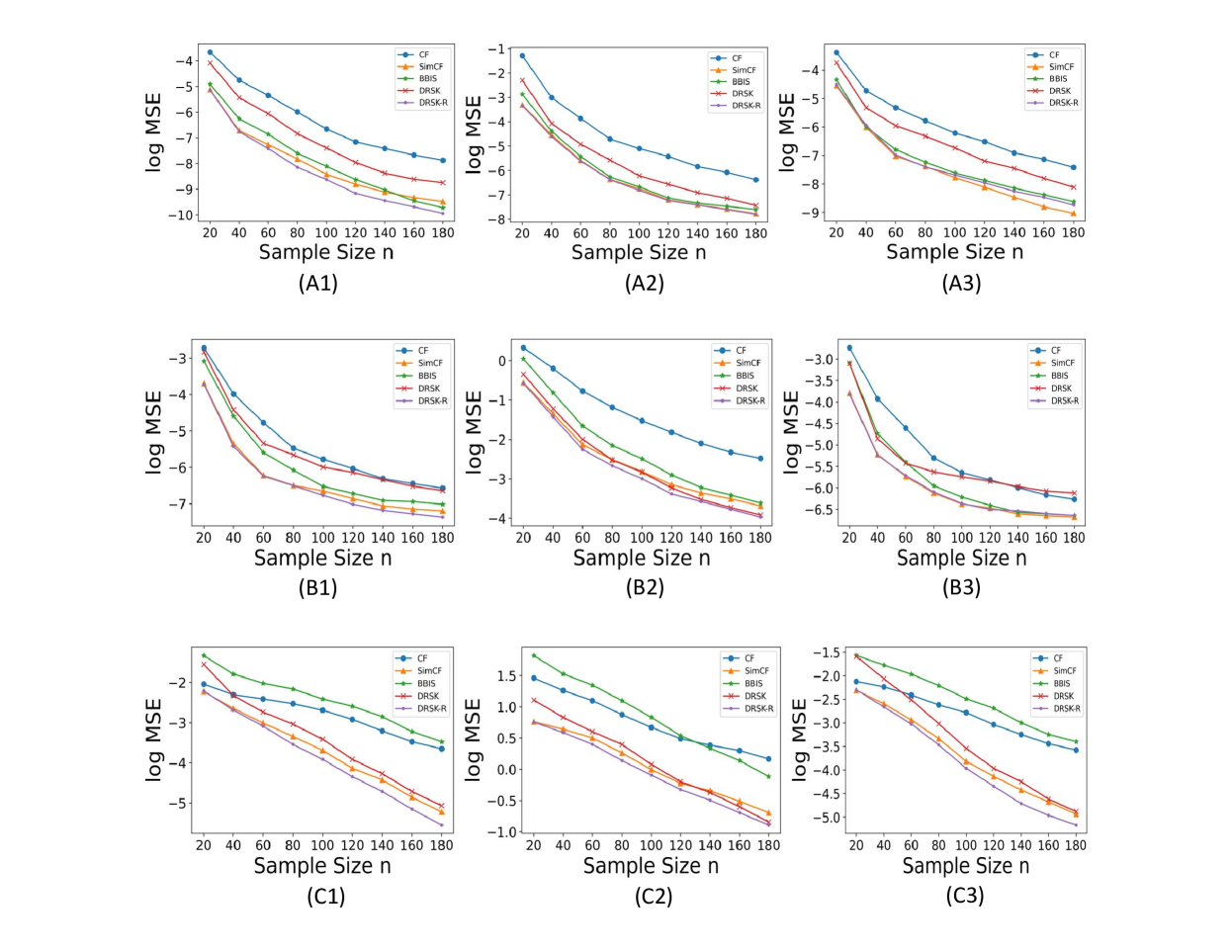
Figure 1: Illustration of different scenarios: The title of the Plot (A1) means the combination of noise setting (1) and biased distribution setting (A). The rest is similar. (1) $\pi_{Y|X}=0$, (2) $\pi_{Y|X}=\mathcal{N}(0,0.1^{2})+\sum_{i=1}^{d}X_{i}$, (3) $\pi_{Y|X}=\mathcal{N}(0,0.1^{2})$. (A) $q_{X}=\pi_{X}$, (B) $q_{X}=\mathcal{N}(0.5,1)$, (C) $q_{X}=\mathcal{N}(1,1)$.

The results are shown in Figure 1. We observe that

1. DRSK-R and SimCF are the top two approaches in most scenarios. Empirically, DRSK-R appears to be a better alternative to DRSK, and SimCF appears to be a better alternative to CF.

2. DRSK-R is the best when the sampling distribution is biased (e.g., biased distribution setting (C)) and the noise is small (e.g., noise setting (1)); See Plots (A1), (B1), (B2), (C1), (C2), (C3). In these scenarios, it can outperform SimCF (the second-best approach) by up to 25 percent.

3. The superior performance of DRSK-R decreases when the sampling distribution is exact or the noise becomes larger; See Plots (A2), (A3), (B3). In (A2) and (B3), DRSK-R and SimCF perform similarly. (A3) is the only scenario where DRSK-R is less effective than SimCF.

These observations coincide with our theory. DRSK (DRSK-R) performs well, especially when the noise is small and the sampling distribution is not exact, consistent with our Table 1. As discussed in Section 3.1, CF (SimCF) is resistant to noise since it takes advantage of the functional approximation of $f$ while the importance weight in BBIS ignores $f$. Thus, increasing noise typically hurts the performance of BBIS, but DRSK (DRSK-R) and CF (SimCF) can maintain some similarly good performance. On the other hand, CF is not resistant to bias because the uniform weight in the final step of constructing CF cannot reduce the bias effectively. Thus SimCF by omitting the final step is a better alternative to CF. Note that this observation holds in almost all scenarios regardless of the bias (including the subsequent experiments). In fact, Oates et al. (2017) indicates a similar empirical result: In the “standard” case, although the CF-adjusted sample $f_{m}(x_{j})$ is constructed for the unbiasedness, the actual bias in $s_{m}(x_{j})$ can be negligible for practical purposes, and thus they recommended SimCF for use in applications. In the “Biased” case, even the unbiasedness of $f_{m}(x_{i})$ is no longer valid so SimCF stays preferable.

Illustration of Different Hyperparameters. We study the effect of different choices of hyperparameters $h_{1}$, $\lambda$ and $B_{0}$ in the scenario (C3): $\pi_{Y|X}=\mathcal{N}(0,0.1^{2})$ and $q_{X}=\mathcal{N}(1,1)$. Let $PSD$ denote the median of the pairwise square distance of the input data. Let $\lambda=a_{1}\times m^{-\frac{1}{2}}$, $h_{1}=a_{2}\times PSD$.

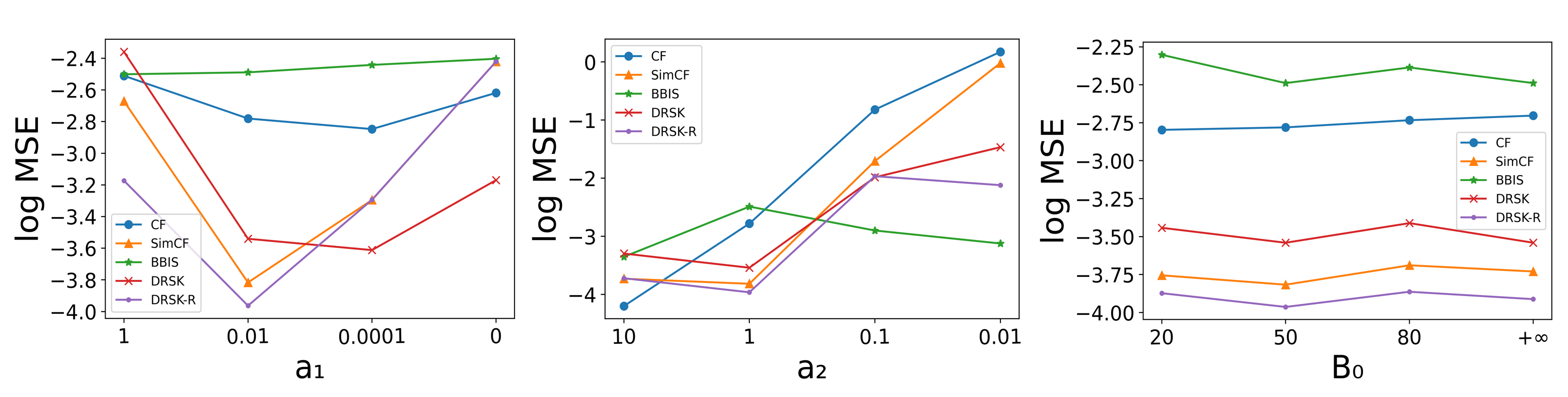
Figure 2: Illustration of different hyperparameters: $\lambda=a_{1}\times m^{-\frac{1}{2}}$, $h_{1}=a_{2}\times PSD$.

The results are shown in Figure 2. We observe that

1. $\lambda=0.01m^{-\frac{1}{2}}$ with $a_{1}=0.01$ appears to be a reasonable choice. Larger or smaller choices of $\lambda$ such as $\lambda=m^{-\frac{1}{2}}$ or $\lambda=0$ produce less satisfactory performance. In particular, $\lambda>0$ is recommended to prevent overfitting and stabilize the inverse numerically.

2. $h_{1}=a_{2}\times PSD$ with $a_{2}=1$ is the choice recommended by previous studies (Liu and Lee, 2017; Gretton et al., 2012). We recognize that other choices of $h_{1}$ may be better. However, tunning $h_{1}$ is not easy in practice. Note that unlike Oates et al. (2017), $h_{1}$ cannot be selected via cross validation in our problem setting because the biased generated distribution does not allow accurate estimation of $\theta$ on the validation data. We have tried some alternative validation approaches such as minimizing variance from different subset divisions but did not see any consistent gain from validation. Therefore, we follow the choice from these previous studies (Liu and Lee, 2017; Gretton et al., 2012).

3. $B_{0}$ is an insensitive hyperparameter. Different choices of $B_{0}$, including the “$+\infty$” in the original BBIS, produce very similar results as long as $B_{0}$ is relatively large.

4.2 Results on a Range of Problems

In this section, we conduct experiments on a variety of data distributions ranging from light-tailed (e.g., the mixture of Gaussian distribution) to heavy-tailed distributions (e.g., t-distribution). Moreover, we consider different dimensions of the input data to show the dimensionality effect on each estimator: $d=1,2,4$.

Throughout the following experiments, the ground-truth $\theta$ is obtained by drawing $10^{6}$ i.i.d. samples $(x_{i},y_{i})$ from the target distribution $\pi$ and calculating the sample average $\theta=\frac{1}{10^{6}}\sum_{i=1}^{10^{6}}f(x_{i},y_{i})$. The hyperparemeters are chosen based on the discussion at the beginning of Section 4.

Mixture of Gaussian Distributions: Suppose $\pi_{X}$ is the pdf of $(0.7\times\mathcal{N}(2,1)+0.3\times\mathcal{N}(1,1))^{\otimes d}$ (^⊗d represents d-dimensional independent component), $q_{X}$ is the pdf of $(\mathcal{N}(1,1))^{\otimes d}$. $\pi_{Y|X}=q_{Y|X}$ is the distribution of $\mathcal{N}(0,0.001^{3})$. Our goal is to compute the expectation of $f(X,Y)=\sin(\frac{\pi}{d}\sum_{i=1}^{d}X_{i})+Y$ under the distribution of $\pi$. The results are displayed in Figure 3.

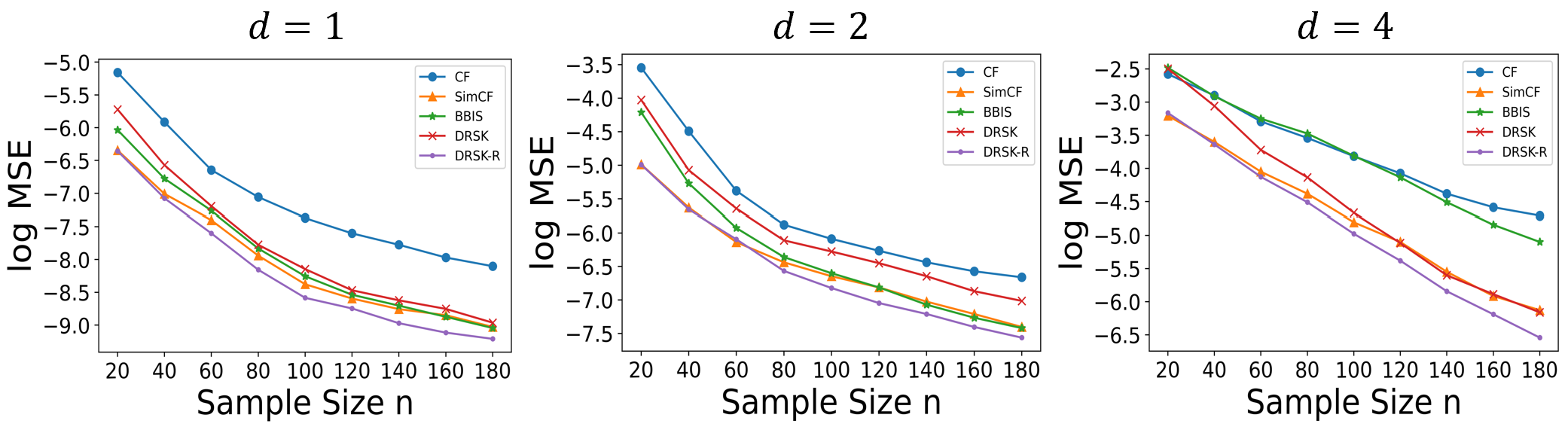
Figure 3: Comparisons of different methods on mixture of Gaussian distributions.

Generalized Student’s T-distributions: Suppose $\pi_{X}$ is the pdf of $(t_{3}(1,1))^{\otimes d}$ ($t_{3}(1,1)=1+1\times t_{3}$ where $t_{3}$ is the standard t-distribution with $3$ degrees of freedom) and $q_{X}$ is the pdf of $\mathcal{N}(\textbf{1},I_{d})$. $\pi_{Y|X}=q_{Y|X}$ is the distribution of $\mathcal{N}(0,0.001^{3})$. Our goal is to compute the expectation of $f(X,Y)=\cos(\frac{\pi}{d}\sum_{i=1}^{d}X_{i})+Y$ with respect to the distribution of $\pi$. The results are displayed in Figure 4.

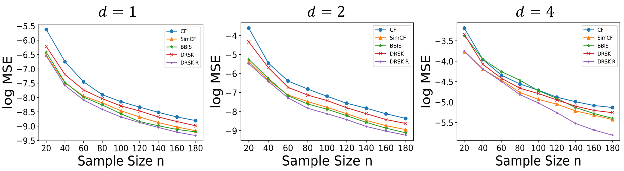
Figure 4: Comparisons of different methods on generalized Student’s t-distributions.

Next, we consider a couple of Bayesian problems. Here, for each problem, we are interested in computing an expectation under the posterior distribution of an unknown input parameter. Typically in a realistic Bayesian setting, we do not have the exact form of the posterior distribution but can obtain it up to a normalizing constant. To simulate the posterior, we draw samples by running the parallel Metropolis–Hastings MCMC algorithm (Liu and Lee, 2017; Rosenthal, 2000). To be specific, suppose we want to draw $n$ samples $x_{i}$ ($i\in[n]$):

1. Draw $n$ i.i.d. samples $x^{0}_{i}$ ($i\in[n]$) from the prior distribution;

2. For each $i$ ($i\in[n]$), run Metropolis-Hastings MCMC algorithm with a symmetric Gaussian proposal kernel starting from $x^{0}_{i}$, which produces $n$ independent Markov chains;

3. For each $i$ ($i\in[n]$), take the endpoint after a finite number of iterations (e.g., 50 iterations) from the $i$-th Markov chains as $x_{i}$.

Obviously, this algorithm will end up with a biased distribution $x_{i}\sim q_{X}$ instead of $\pi_{X}$. Moreover, $x_{1},\cdots,x_{n}$ are independent because they are from different Markov chains.

In the following experiments, to be able to validate our estimators against the ground truth, we consider conjugate distributions so that the posterior distribution can be derived explicitly. Note that this information is only used to obtain the ground-truth $\theta$ for evaluation, but not used for constructing the estimators.

Gamma Conjugate Distributions: Suppose $x$ is an unknown input parameter. Let $x$ have a prior distribution $p_{0}(x)=(\text{Gamma}(2,2))^{\otimes d}$ (a Gamma distribution with a shape parameter $2$ and a rate parameter $2$). To estimate $x$, collect a set of data $\Xi=\{\xi^{(l)}=(\xi_{1}^{(l)},\cdots,\xi_{d}^{(l)}):l=1,\cdots,L\}$ which are i.i.d. drawn from the likelihood $p(\Xi|x)=(\text{Gamma}(4,x))^{\otimes d}$ (a Gamma distribution with a shape parameter $4$ and a rate parameter $x$). The distribution of interest is the posterior distribution, which is $\text{Gamma}(4L+2,\sum_{l=1}^{L}\xi_{1}^{(l)}+2)\otimes\cdots\otimes\text{Gamma}(4L+2,\sum_{l=1}^{L}\xi_{d}^{(l)}+2)$ as it is a conjugate distribution. To mimic $\pi_{X}$, $q_{X}$ is obtained by running the parallel Metropolis–Hastings MCMC algorithm as described in this Section. $\pi_{Y|X}=q_{Y|X}$ is the distribution of $\mathcal{N}(0,0.001^{3})$. Suppose $L=12$ and $\sum_{l=1}^{L}\xi_{i}^{(l)}=3+5i$. Our goal is to compute the expectation of $f(X,Y)=\sin(\frac{\pi}{d}\sum_{i=1}^{d}X_{i})+Y$ under the distribution $\pi$. The results are displayed in Figure 5.

Figure 5: Comparisons of different methods on Gamma conjugate distributions.

Beta Conjugate Distribution: Suppose $x$ is an unknown input parameter. Let $x$ have a prior distribution $p_{0}(x)=(\text{Beta}(1,1))^{\otimes d}$ (a Beta distribution with two shape parameters $1$ and $1$). To estimate $x$, collect a set of data $\Xi=\{\xi^{(l)}=(\xi_{1}^{(l)},\cdots,\xi_{d}^{(l)}):l=1,\cdots,L\}$ which are i.i.d. drawn from the likelihood $p(\Xi|x)=\text{Bernoulli}(x)$ where the “success” parameter is $x$. The distribution of interest is the posterior distribution $\pi_{X}(x)\propto p(\Xi|x)p_{0}(x)$, which is $\text{Beta}(\sum_{l=1}^{L}y_{1}^{(l)}+1,L-\sum_{l=1}^{L}y_{1}^{(l)}+1)\otimes\cdots\otimes\text{Beta}(\sum_{l=1}^{L}y_{d}^{(l)}+1,L-\sum_{l=1}^{L}y_{d}^{(l)}+1)$ as it is a conjugate distribution. To mimic $\pi_{X}$, $q_{X}$ is obtained by running the parallel Metropolis–Hastings MCMC algorithm as described in this Section. $\pi_{Y|X}=q_{Y|X}$ is the distribution of $\mathcal{N}(0,0.001^{3})$. Suppose $L=11$ and $\sum_{l=1}^{L}y_{i}^{(l)}=1+i$. Our goal is to compute the expectation of $f(X,Y)=\cos(\frac{\pi}{d}\sum_{i=1}^{d}X_{i})+Y$ under the distribution $\pi$. The results are displayed in Figure 6.

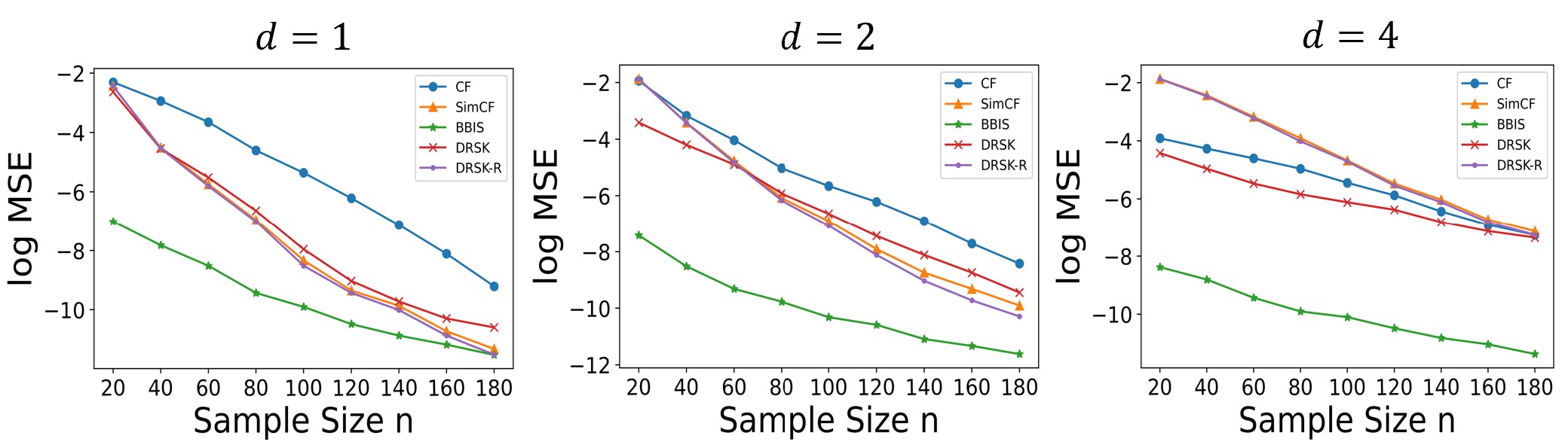
Figure 6: Comparisons of different methods on Beta conjugate distributions.

Finally, we consider a stochastic simulation experiment, under input uncertainty where the modeler needs to provide performance measure estimate that accounts for both the aleatory noise from the simulation model and the epistemic noise from the input parameter that is handled via Bayesian posterior.

Computer Communication Network: We conduct experiments on a computer communication network example borrowed from Lam and Qian (2021); Lin et al. (2015). Figure 7 illustrates the structure of this computer communication network. It consists of 4 message-processing units (nodes) which are connected by 4 transport channels (edges). There are external messages that will enter the network. We assume that the lengths of the external messages are i.i.d. and follow an exponential distribution with rate $\frac{1}{300}$. For every pair $(i,j)$ of nodes ($i\neq j$), external messages arriving at node $i$ that are to be transmitted to node $j$ follow a Poisson arrival process with an unknown rate $\lambda_{i,j}$ where their transmission path is fixed and known. Suppose that each node takes a constant time of $0.001$ seconds to process a message with unlimited storage capacity, and each edge has a capacity of 275000 bits. All messages transmit through the edges with a constant velocity of 150000 miles per second, and the $i$-th edge has a length of $100i$ miles for $i=1,2,3,4$. Therefore, the total time that a message of length $l$ bits occupies the $i$-th edge is $\frac{l}{275000}+\frac{100i}{150000}$ seconds. Suppose that the computer network is empty at time zero.

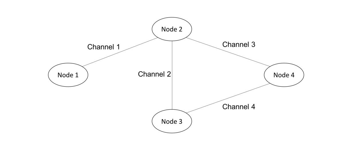
Figure 7: A computer communication network with four nodes and four channels.

Setting (A) 1 2 3 4 1 n.a. 0.5 0.7 0.6 2 0.4 n.a. 0.4 1.2 3 0.3 1.2 n.a. 1.0 4 0.8 0.7 0.5 n.a.   Setting (B) 1 2 3 4 1 n.a. 0.3 0.5 0.4 2 0.2 n.a. 0.3 1.1 3 0.2 1.0 n.a. 0.9 4 0.5 0.4 0.3 n.a.   Setting (C) 1 2 3 4 1 n.a. 0.4 0.6 0.5 2 0.3 n.a. 0.4 1.0 3 0.3 1.2 n.a. 0.7 4 0.6 0.5 0.4 n.a.

Table 2: Interarrival times for estimating the arrival rates $\lambda_{i,j}$. These tables report the cumulative value of $0.1+\sum_{l=1}^{L}\xi^{(l)}_{i,j}$ where $L=10$ and $i,j=1,\cdots,4$ in three different settings of ground-truth $\lambda$.

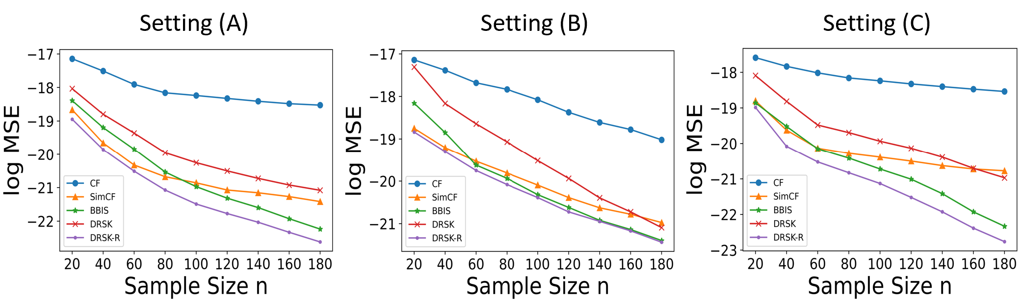
Figure 8: Comparisons of different methods on the computer communication network. Settings (A),(B),(C) correspond to the different data in Table 2 with different settings of ground-truth $\lambda$.

The value of interest is the delay of the first 30 messages that arrive in the system, or $\frac{1}{30}\sum_{i=1}^{30}T_{k}$, where $T_{k}$ is the time that the $k$-th message takes to be transmitted from its entering node to destination node. To estimate this value, for each input rate vector $\lambda=(\lambda_{i,j})_{i,j=1,2,3,4;i\neq j}\in\mathbb{R}_{+}^{12}$, we simulate the system $100$ times and take the average $f(\lambda,Y):=\frac{1}{100}\sum_{j=1}^{100}\frac{1}{30}\sum_{i=1}^{30}T^{(j)}_{k}(\lambda)$ as our simulation output. Here, $T^{(j)}_{k}(\lambda)$ is the delay of the $k$-th message in the $j$-th simulation when the input rate vector is given by $\lambda$. Obviously, $f(\lambda,Y)$ depends on not only $\lambda$, but also the stochasticity in the simulation model, denoted as $Y$ (since $T^{(j)}_{k}$ is a random output from the simulation model). Let $\pi_{Y|\lambda}$ denote the distribution of $Y$ given $\lambda$.

We apply Bayesian inference to estimate the unknown arrival rate vector $\lambda$. First we endow $\lambda$ with a prior distribution $(\text{Gamma}(10,0.1))^{\otimes d}$. By the definition of $\lambda$, the interarrival time of the external messages arriving at node $i$ that are to be transmitted to node $j$, denoted as $\xi_{i,j}$, follow an exponential distribution with rate $\lambda_{i,j}$. To infer $\lambda$, we collect some historical data of the interarrival times $\xi^{(1)}_{i,j},\cdots,\xi^{(L)}_{i,j}$ and use them to update the posterior distribution of $\lambda_{i,j}$. Suppose $L=10$. These data are summarized in Table 2, each obtained from a different setting of ground-truth $\lambda$.

The exact posterior distribution of $\lambda$, denoted as $\pi_{\lambda}$, is known to be $\text{Gamma}(10+L,\sum_{l=1}^{L}\xi_{1,2}^{(l)}+0.1)\otimes\cdots\otimes\text{Gamma}(10+L,\sum_{l=1}^{L}\xi_{4,3}^{(l)}+0.1)$. Let $\pi:=\pi_{\lambda}\pi_{Y|\lambda}$. However, this information is only used to obtain the ground-truth $\theta:=\mathbb{E}_{\pi}[f(\lambda,Y)]$ (by drawing $10^{6}$ i.i.d. samples as we discussed at the beginning of Section 4.2), but not used for constructing the estimators. To construct the estimators, we run the parallel Metropolis–Hastings MCMC algorithm as described in this Section to mimic the posterior, obtain i.i.d. samples $\lambda^{(1)},\cdots,\lambda^{(n)}\sim q_{\lambda}$ with sample size $n$, and plug into $f(\lambda^{(i)},Y)$ ($i\in[n]$). The results are displayed in Figure 8.

We conclude our findings from the numerical results.

1. Overall, our experiments illustrate the high effectiveness of our estimators DRSK-R (DRSK) in terms of reducing the MSE in Monte Carlo computation. DRSK-R appears to be a better alternative to DRSK, outperforming DRSK in almost all experiments.

2. The relative performance of DRSK-R compared with other methods is stable. DRSK-R maintains superior performance regardless of the dimension of the input data, up to 12 in the real-world computer communication network example. In some cases (e.g., Figures 3 and 4), its superiority becomes more distinct when the dimension increases. In addition, DRSK-R achieves better results than CF and SimCF in almost all experiments. DRSK-R outperforms BBIS in most experiments while the relative performance of BBIS tends to be variable among different experiments.

3. In the realistic computer communication network example consisting of 12 estimated input parameters and a sophisticated black-box simulation model, the experiments indicate that our DRSK-R achieves the best results consistently across multiple model settings and also shows its better relative performance against CF (SimCF).

4. DRSK-R may be less effective when the sampling distribution is exact (e.g., Plot (A3) in Figure 1), or for some specific target distributions (e.g., Beta distributions in Figure 6). It may sometimes perform similarly to BBIS (e.g., Setting (A2) in Figure 8) or SimCF (e.g., Setting (B3) in Figure 1). Nevertheless, by taking advantage of both CF and BBIS, it achieves the smallest MSE in most experiments.

5 Theory for Regularized Least Square Regression

In this section, we first review basic facts about RLS regression (aka KRR), whose framework follows Smale and Zhou (2005) and Sun and Wu (2009). Next, we develop some theoretical results for the purpose of our analysis in Section 6.

Suppose we have i.i.d. samples $\{(x_{j},f(x_{j},y_{j})):j=1,\cdots,m\}$ where $(x_{i},y_{i})$ are i.i.d. drawn from the sampling distribution $q$. We denote $\hat{z}=(f(x_{1},y_{1}),\cdots,f(x_{m},y_{m}))^{T}$. We call $f_{q}$ the (ground-truth) regression function defined by

$$f_{q}(x)=\mathbb{E}_{q}[f(X,Y)|X=x].$$

The goal of KRR is to learn the regression function by constructing a “good” approximating function $s_{m}$ from the data. Let $\mathcal{H}$ be a generic RKHS with the associated kernel $k(x,y)$. Let $\|\cdot\|_{\mathcal{H}}$ denote the norm on $\mathcal{H}$. Note that $k_{x}=k(x,\cdot)$ is a function in $\mathcal{H}$.

For this section, we only impose the following assumption:

Assumption 6

$\kappa:=\sup_{x\in\Omega}\sqrt{k(x,x)}<\infty$, $M_{0}:=\mathbb{E}_{q}[(z-f_{q}(x))^{2}]<\infty$. For any $g\in\mathcal{H}$, $g(x)$ is $q$-measurable. $f_{q}\in L^{2}(q_{X})$.

It follows that for any $g\in\mathcal{H}$,

$$\sup_{t\in\Omega}|g(t)|^{2}=\sup_{t\in\Omega}|\langle g,k_{t}\rangle|^{2}\leq\sup_{t\in\Omega}\|g\|^{2}_{\mathcal{H}}\|k_{t}\|^{2}_{\mathcal{H}}\leq\kappa^{2}\|g\|^{2}_{\mathcal{H}}.$$

So under Assumption 6, any $g\in\mathcal{H}$ is a bounded function. We point out the following inequality that we will use frequently:

$$\|g\|_{L^{p}(q_{X})}\leq\kappa\|g\|_{\mathcal{H}},\quad\forall 1\leq p\leq\infty.$$ (15)

The RLS problem is given by

$$s_{m}(x):=\mathop{\arg\min}_{g\in\mathcal{H}}\left\{\frac{1}{m}\sum_{j=1}^{m}(f(x_{j},y_{j})-g(x_{j}))^{2}+\lambda\|g\|^{2}_{\mathcal{H}}\right\}$$

where $\lambda>0$ is a regularization parameter which may depend on the cardinality of the training data set. Note that the data needed in this problem are only the values $\{x_{j}\}_{j=1,\cdots,m}$ and $\{z_{j}:=f(x_{j},y_{j})\}_{j=1,\cdots,m}$, so $y_{j}$ and $f$ can be in a black box. A nice property of RLS is that there is an closed-form formula for its solution, as stated below.

Lemma 9

Let $K=(k(x_{i},x_{j}))_{m\times m}\in\mathbb{R}^{m\times m}$ be the kernel Gram matrix and

$$\hat{k}(x)=(k(x_{1},x),\cdots,k(x_{m},x))^{T}.$$

Then the RLS solution is given as $s_{m}(x)=\beta^{T}\hat{k}(x)$ where $\beta=(K+\lambda mI)^{-1}\hat{z}$.

Lemma 9 shows a direct way to calculate $s_{m}$. From a theoretical point of view, to derive the property of $s_{m}$, we need to use some tools from functional analysis. To begin, we give an equivalent form of $s_{m}$ in terms of linear operators. Define the sampling operator $S_{x}:\mathcal{H}\to\mathbb{R}^{m}$ associated with a discrete subset $\{x_{i}\}^{m}_{i=1}$ by

$$S_{x}(g)=(g(x_{i}))^{m}_{i=1},\ g\in\mathcal{H}.$$

The adjoint of the sampling operator, $S^{T}_{x}:\mathbb{R}^{m}\to\mathcal{H}$, is given by

$$S^{T}_{x}(c)=\sum_{i=1}^{m}c_{i}k_{x_{i}},c\in\mathbb{R}^{m}.$$

Note that the compound mapping $S^{T}_{x}S_{x}$ is a positive self-adjoint operator on $\mathcal{H}$. Let $I$ denote the identity mapping on $\mathcal{H}$. We have:

Lemma 10

The RLS solution can be written as follows:

$$s_{m}=\left(\frac{1}{m}S^{T}_{x}S_{x}+\lambda I\right)^{-1}\frac{1}{m}S^{T}_{x}(\hat{z}).$$

A proof can be found in Smale and Zhou (2005). It is also easy to derive this result directly from Lemma 9.

Denote

$$\mathcal{H}_{0}^{q}:=\{g\in\mathcal{H}:g=0\ \text{ a.e. with respect to }q\}\ \text{and}$$

$$\mathcal{H}_{1}^{q}:=(\mathcal{H}_{0}^{q})^{\perp}\text{, the orthogonal complement of }\mathcal{H}_{0}^{q}\text{ in }\mathcal{H}.$$

If $q$ is clear from the context, we write $\mathcal{H}_{0}=\mathcal{H}_{0}^{q}$, $\mathcal{H}_{1}=\mathcal{H}_{1}^{q}$ for simplicity. Note that both $\mathcal{H}_{0}$ and $\mathcal{H}_{1}$ are closed subspaces in $\mathcal{H}$ with respect to the norm $\|\cdot\|_{\mathcal{H}}$. It is well-known that $\mathcal{H}/\mathcal{H}_{0}$ is isometrically isomorphic to $\mathcal{H}_{1}$. So $\mathcal{H}_{1}$ is essentially the quotient space of $\mathcal{H}$ induced by the equivalence relation “a.e. with respect to $q$”, the same equivalence relation in $L^{2}(q_{X})$. If $f\in\mathcal{H}$, we may replace the original $f\in\mathcal{H}$ with a equivalent $\tilde{f}\in\mathcal{H}_{1}$ ($f=\tilde{f}$ a.e. with respect to $q$) since this will not effect the estimation of the parameter. For this purpose, we may treat $\mathcal{H}_{1}$ as $\mathcal{H}$. (But they are substantially different in some way, see Sun and Wu (2009).) Let $\overline{\mathcal{H}_{1}}^{q}$ (which is the same as $\overline{\mathcal{H}}^{q}$) be the closure of $\mathcal{H}_{1}$ in $L^{2}(q_{X})$.

Next, we introduce a standard result from functional analysis. This result can be found in Theorem 2.4 and Proposition 2.10 in Sołtan (2018).

Theorem 11

Let $A$ be a bounded self-adjoint linear operator. Let $C(\sigma(A))$ be the set of real-valued continuous functions defined on the spectrum of $A$. Then for any $g\in C(\sigma(A))$, $g(A)$ is self-adjoint and $\|g(A)\|=\sup_{x\in\sigma(A)}|g(x)|.$

Define $L_{q}:L^{2}(q_{X})\to L^{2}(q_{X})$ as the integral operator

$$(L_{q}g)(x):=\int_{\Omega}k(x,x^{\prime})g(x^{\prime})q(x^{\prime})dx^{\prime},\ x\in\Omega,\ g\in L^{2}(q_{X}).$$

This operator can be viewed as a linear operator on $L^{2}(q_{X})$ or on $\mathcal{H}$. Unless specified otherwise, we always assume the domain of $L_{q}$ is $L^{2}(q_{X})$. Sun and Wu (2009) shows that $L_{q}$ is a compact and positive self-adjoint operator on $L^{2}(q_{X})$. Theorem 11 shows that $L_{q}^{r}$ is a well-defined self-adjoint operator on $L^{2}(q_{X})$ for $0\leq r\leq 1$. Denote $\text{Range}(L_{q}^{r})$ the range of $L_{q}^{r}$ on the domain $L^{2}(q_{X})$. When we write $L_{q}^{-r}g\in L^{2}(q_{X})$, it should be understood that (1) $g\in\text{Range}(L_{q}^{r})$, (2) $L_{q}^{-r}g$ is an element in the preimage set of $g$ under the operator $L_{q}^{r}$ on the domain $L^{2}(q_{X})$.

We will frequently use the following lemma, which indicates a useful property of the integral operator $L_{q}$ (a proof can be found in Sun and Wu (2009)).

Lemma 12

$L_{q}^{\frac{1}{2}}f\in\mathcal{H}_{1}$ for any $f\in L^{2}(q_{X})$, and $L_{q}^{\frac{1}{2}}$ is an isometric isomorphism from $(\overline{\mathcal{H}_{1}}^{q},\|\cdot\|_{L^{2}(q_{X})})$ onto $(\mathcal{H}_{1},\|\cdot\|_{\mathcal{H}})$.

Note that Lemma 12 implies that $\text{Range}(L_{q}^{\frac{1}{2}})=\text{Range}(L_{q}^{\frac{1}{2}}|_{\overline{\mathcal{H}_{1}}^{q}})=\mathcal{H}_{1}$.

Next, consider an oracle or a data-free limit of $s_{m}$ as

$$f_{\lambda}:=\mathop{\arg\min}_{g\in\mathcal{H}}\left\{\|g-f_{q}\|^{2}_{L^{2}(q_{X})}+\lambda\|g\|^{2}_{\mathcal{H}}\right\}.$$

We have the following explicit expression (a proof can be found in Cucker and Smale (2002a)):

Lemma 13

The solution of $f_{\lambda}$ is given as $f_{\lambda}=(L_{q}+\lambda I)^{-1}L_{q}f_{q}$.

To show that $s_{m}-f_{q}$ is small, we split it into two parts

$$s_{m}-f_{q}=(s_{m}-f_{\lambda})+(f_{\lambda}-f_{q}).$$ (16)

The first part in (16) comes from the statistical noise in the RLS regression, whereas the second part can be viewed as the bias of the functional approximation. In terms of terminology in machine learning, the first term is called the estimation error (or sample error) and the second term called the approximation error. We study the asymptotic error of each part in the next set of results.

Proposition 14

Suppose that $L_{q}^{-r}f_{q}\in L^{2}(q_{X})$ where $0\leq r\leq 1$. Then
(1) $\|f_{\lambda}-f_{q}\|_{L^{2}(q_{X})}\leq\lambda^{r}\|L_{q}^{-r}f_{q}\|_{L^{2}(q_{X})}$.
(2) $\|f_{\lambda}-f_{q}\|_{\mathcal{H}}\leq\lambda^{r-\frac{1}{2}}\|L_{q}^{-r}f_{q}\|_{L^{2}(q_{X})}$ for $\frac{1}{2}\leq r\leq 1$ only.

Proof  We remark that $\|L_{q}^{-r}f_{q}\|_{L^{2}(q_{X})}$ measures a complexity of the regression function (Smale and Zhou, 2007). Using Lemma 13, we write

$$f_{\lambda}-f_{q}=(L_{q}+\lambda I)^{-1}L_{q}f_{q}-f_{q}=-\lambda(L_{q}+\lambda I)^{-1}f_{q}.$$

(1) For the first part, we write

$$\|f_{\lambda}-f_{q}\|_{L^{2}(q_{X})}=\lambda\|(L_{q}+\lambda I)^{-1}L_{q}^{r}L_{q}^{-r}f_{q}\|_{{}_{L^{2}(q_{X})}}\leq\lambda\|(L_{q}+\lambda I)^{-1}L_{q}^{r}\|\|L_{q}^{-r}f_{q}\|_{{}_{L^{2}(q_{X})}}.$$

Here we regard $L_{q}$ as a bounded positive self-adjoint operator on $L^{2}(q_{X})$. Then Theorem 11 states that $\|(L_{q}+\lambda I)^{-1}L_{q}^{r}\|\leq\|h\|_{\infty}$ where $h(x)=\frac{x^{r}}{x+\lambda}$ is defined on $x\in[0,\infty)$ ($L_{q}$ is positive so $\sigma(L_{q})\subset[0,\infty)$). Note that $\|h\|_{\infty}\leq\lambda^{r-1}$. So

$$\|f_{\lambda}-f_{q}\|_{L^{2}(q_{X})}\leq\lambda\lambda^{r-1}\|L_{q}^{-r}f_{q}\|_{{}_{L^{2}(q_{X})}}^{2}=\lambda^{r}\|L_{q}^{-r}f_{q}\|_{L^{2}(q_{X})}.$$

(2) For the second part, we exhibit an intuitive proof here. We write

$$\|f_{\lambda}-f_{q}\|_{\mathcal{H}}=\lambda\|L_{q}^{\frac{1}{2}}L_{q}^{-\frac{1}{2}}(L_{q}+\lambda I)^{-1}f_{q}\|_{\mathcal{H}}=\lambda\|L_{q}^{-\frac{1}{2}}(L_{q}+\lambda I)^{-1}f_{q}\|_{L^{2}(q_{X})}.$$

The last equality is intuitively correct due to Lemma 12. (However, this statement is not rigorous because $L_{q}^{-\frac{1}{2}}(L_{q}+\lambda I)^{-1}f_{q}$ is not necessarily in $\overline{\mathcal{H}_{1}}^{q}$. A rigorous argument can be found in Sun and Wu (2009).) Next we notice that

$$\|L_{q}^{-\frac{1}{2}}(L_{q}+\lambda I)^{-1}f_{q}\|_{L^{2}(q_{X})} =\|L_{q}^{-\frac{1}{2}}(L_{q}+\lambda I)^{-1}L_{q}^{r}L_{q}^{-r}f_{q}\|_{L^{2}(q_{X})}$$

$$\leq\|L_{q}^{-\frac{1}{2}}(L_{q}+\lambda I)^{-1}L_{q}^{r}\|\|L_{q}^{-r}f_{q}\|_{L^{2}(q_{X})}.$$

Theorem 11 states that $\|L_{q}^{-\frac{1}{2}}(L_{q}+\lambda I)^{-1}L_{q}^{r}\|\leq\|h\|_{\infty}$ where $h(x)=\frac{x^{r-\frac{1}{2}}}{x+\lambda}$ is defined on $x\in[0,\infty)$ ($L_{q}$ is positive so $\sigma(L_{q})\subset[0,\infty)$). Note that $\|h\|_{\infty}\leq\lambda^{r-\frac{3}{2}}$. So

$$\|f_{\lambda}-f_{q}\|_{\mathcal{H}}\leq\lambda\lambda^{r-\frac{3}{2}}\|L_{q}^{-r}f_{q}\|_{L^{2}(q_{X})}=\lambda^{r-\frac{1}{2}}\|L_{q}^{-r}f_{q}\|_{L^{2}(q_{X})}.$$

 

If we want to obtain a better bound for $f_{\lambda}-f_{q}$ by using this proposition, we may want $r$ to be as large as possible, but meanwhile $L_{q}^{-r}f_{q}\in L^{2}(q_{X})$ becomes a more restrictive constraint. However, we have the following proposition that can bypass this tradeoff.

Proposition 15

The range of $L_{q}$ satisfies

$$\overline{\text{Range}(L_{q})}^{q}=\overline{\text{Range}(L_{q}|_{\overline{\mathcal{H}_{1}}^{q}})}^{q}=\overline{\mathcal{H}_{1}}^{q}(=\overline{\mathcal{H}}^{q}).$$

Proof  Take any $f_{1}\in\overline{\mathcal{H}_{1}}^{q}$. For any $\epsilon>0$, there exists $f_{2}\in\mathcal{H}_{1}$ such that $\|f_{1}-f_{2}\|_{L^{2}(q_{X})}\leq\epsilon$. It follows from Lemma 12 that there exists $g_{1}\in\overline{\mathcal{H}_{1}}^{q}$ such that $L_{q}^{\frac{1}{2}}g_{1}=f_{2}$. There exists $g_{2}\in\mathcal{H}_{1}$ such that $\|g_{1}-g_{2}\|_{L^{2}(q_{X})}\leq\frac{\epsilon}{\kappa}$. Again, it follows from Lemma 12 that there exists $h_{1}\in\overline{\mathcal{H}_{1}}^{q}$ such that $L_{q}^{\frac{1}{2}}h_{1}=g_{2}$. Then we have

$$\|L_{q}h_{1}-f_{2}\|_{L^{2}(q_{X})}\leq\kappa\|L_{q}h_{1}-f_{2}\|_{\mathcal{H}}=\kappa\|L_{q}^{\frac{1}{2}}g_{2}-L_{q}^{\frac{1}{2}}g_{1}\|_{\mathcal{H}}=\kappa\|g_{2}-g_{1}\|_{L^{2}(q_{X})}\leq\epsilon$$

and

$$\|L_{q}h_{1}-f_{1}\|_{L^{2}(q_{X})}\leq\|L_{q}h_{1}-f_{2}\|_{L^{2}(q_{X})}+\|f_{2}-f_{1}\|_{L^{2}(q_{X})}\leq 2\epsilon.$$

This implies that $f_{1}\in\overline{\text{Range}(L_{q}|_{\overline{\mathcal{H}_{1}}^{q}})}^{q}$ so

$$\overline{\text{Range}(L_{q}|_{\overline{\mathcal{H}_{1}}^{q}})}^{q}\supset\overline{\mathcal{H}_{1}}^{q}.$$

On the other hand, Lemma 12 indicates that

$$\text{Range}(L_{q}|_{\overline{\mathcal{H}_{1}}^{q}})\subset\text{Range}(L_{q})\subset\text{Range}(L_{q}^{\frac{1}{2}})=\mathcal{H}_{1}.$$

Hence we have

$$\overline{\text{Range}(L_{q})}^{q}=\overline{\text{Range}(L_{q}|_{\overline{\mathcal{H}_{1}}^{q}})}^{q}=\overline{\mathcal{H}_{1}}^{q}.$$

 

Denote $\overline{\text{Range}(L_{q})}^{\mathcal{H}}$ the closure of $\text{Range}(L_{q})$ in $\mathcal{H}$ with respect to the norm of $\mathcal{H}$. We have the following similar proposition in terms of the norm in $\mathcal{H}$.

Proposition 16

The range of $L_{q}$ satisfies

$$\overline{\text{Range}(L_{q})}^{\mathcal{H}}=\overline{\text{Range}(L_{q}|_{\overline{\mathcal{H}_{1}}^{q}})}^{\mathcal{H}}=\mathcal{H}_{1}.$$

Proof  Take any $f_{1}\in\mathcal{H}_{1}$. It follows from Lemma 12 that there exists $g_{1}\in\overline{\mathcal{H}_{1}}^{q}$ such that $L_{q}^{\frac{1}{2}}g_{1}=f_{1}$. For any $\epsilon>0$, there exists $g_{2}\in\mathcal{H}_{1}$ such that $\|g_{1}-g_{2}\|_{L^{2}(q_{X})}\leq\epsilon$. Again, it follows from Lemma 12 that there exists $h_{1}\in\overline{\mathcal{H}_{1}}^{q}$ such that $L_{q}^{\frac{1}{2}}h_{1}=g_{2}$ and we have

$$\|L_{q}h_{1}-f_{1}\|_{\mathcal{H}}=\|L_{q}h_{1}-L_{q}^{\frac{1}{2}}g_{1}\|_{\mathcal{H}}=\|L_{q}^{\frac{1}{2}}h_{1}-g_{1}\|_{L^{2}(q_{X})}=\|g_{2}-g_{1}\|_{L^{2}(q_{X})}\leq\epsilon.$$

This implies that $f_{1}\in\overline{\text{Range}(L_{q}|_{\overline{\mathcal{H}_{1}}^{q}})}^{\mathcal{H}}$ so

$$\overline{\text{Range}(L_{q}|_{\overline{\mathcal{H}_{1}}^{q}})}^{\mathcal{H}}\supset\mathcal{H}_{1}.$$

On the other hand, Lemma 12 indicates that

$$\text{Range}(L_{q}|_{\overline{\mathcal{H}_{1}}^{q}})\subset\text{Range}(L_{q})\subset\text{Range}(L_{q}^{\frac{1}{2}})=\mathcal{H}_{1}.$$

Note that $\mathcal{H}_{1}$ is a closed subspace in $\mathcal{H}$. Hence we have

$$\overline{\text{Range}(L_{q})}^{\mathcal{H}}=\overline{\text{Range}(L_{q}|_{\overline{\mathcal{H}_{1}}^{q}})}^{\mathcal{H}}=\mathcal{H}_{1}.$$

 

Propositions 15 and 16 give a theoretical explanation that if we have a result in the space $\text{Range}(L_{q})$, we may anticipate that it is also (approximately) valid in $\overline{\mathcal{H}}^{q}$ or $\mathcal{H}_{1}$.

Proposition 17

We have

$$\|s_{m}-f_{\lambda}\|_{\mathcal{H}}\leq\frac{1}{\lambda}\|\Delta\|_{\mathcal{H}}$$

where

$$\Delta:=\frac{1}{m}\sum_{i=1}^{m}(z_{i}-f_{\lambda}(x_{i}))k_{x_{i}}-L_{q}(f_{q}-f_{\lambda}).$$

Proof  By definition,

$$s_{m}-f_{\lambda}=\left(\frac{1}{m}S^{T}_{x}S_{x}+\lambda I\right)^{-1}\left(\frac{1}{m}S^{T}_{x}(z)-\frac{1}{m}S^{T}_{x}S_{x}f_{\lambda}-\lambda f_{\lambda}\right).$$

Direct computation leads to

$$\frac{1}{m}S^{T}_{x}(z)-\frac{1}{m}S^{T}_{x}S_{x}f_{\lambda}=\frac{1}{m}\sum_{i=1}^{m}(z_{i}-f_{\lambda}(x_{i}))k_{x_{i}},\ \text{and}\ \lambda f_{\lambda}=L_{q}(f_{q}-f_{\lambda})$$

so

$$s_{m}-f_{\lambda}=\left(\frac{1}{m}S^{T}_{x}S_{x}+\lambda I\right)^{-1}\Delta.$$

View $S^{T}_{x}S_{x}$ as a positive self-adjoint operator on $\mathcal{H}$. By Theorem 11, we have

$$\left\|\left(\frac{1}{m}S^{T}_{x}S_{x}+\lambda I\right)^{-1}\right\|_{\mathcal{H}\to\mathcal{H}}\leq\frac{1}{\lambda}.$$

Hence we obtain

$$\|s_{m}-f_{\lambda}\|_{\mathcal{H}}\leq\frac{1}{\lambda}\|\Delta\|_{\mathcal{H}}$$

as desired.  

Next we have the following:

Proposition 18

We have

$$\mathbb{E}_{q}[\|\Delta\|^{2}_{\mathcal{H}}]\leq\frac{1}{m}\kappa^{2}(\nu_{X}((f_{q}-f_{\lambda})^{2})+M_{0}).$$

Proof  Consider

$$\|\Delta\|^{2}_{\mathcal{H}}=\langle\frac{1}{m}\sum_{i=1}^{m}((z_{i}-f_{\lambda}(x_{i}))k_{x_{i}}-L_{q}(f_{q}-f_{\lambda})),\frac{1}{m}\sum_{i=1}^{m}((z_{i}-f_{\lambda}(x_{i}))k_{x_{i}}-L_{q}(f_{q}-f_{\lambda}))\rangle.$$

Direct computation shows that, for the first term,

$$\langle(z_{i}-f_{\lambda}(x_{i}))k_{x_{i}},(z_{j}-f_{\lambda}(x_{j}))k_{x_{j}}\rangle=(z_{i}-f_{\lambda}(x_{i}))(z_{j}-f_{\lambda}(x_{j}))k(x_{i},x_{j})$$

For $i\neq j$, we have

$$\mathbb{E}_{q}\langle(z_{i}-f_{\lambda}(x_{i}))k_{x_{i}},(z_{j}-f_{\lambda}(x_{j}))k_{x_{j}}\rangle$$

$$= \int_{\Omega}\int_{\Omega}(f_{q}(x_{i})-f_{\lambda}(x_{i}))(f_{q}(x_{j})-f_{\lambda}(x_{j}))k(x_{i},x_{j})q(x_{i})q(x_{j})dx_{i}dx_{j}$$

For $i=j$, we have

$$\mathbb{E}_{q}\langle(z_{i}-f_{\lambda}(x_{i}))k_{x_{i}},(z_{j}-f_{\lambda}(x_{j}))k_{x_{j}}\rangle=\mathbb{E}_{q}[(z_{i}-f_{\lambda}(x_{i}))^{2}k(x_{i},x_{i})]$$

For the cross item, we have

$$\langle(z_{i}-f_{\lambda}(x_{i}))k_{x_{i}},L_{q}(f_{q}-f_{\lambda})\rangle=\int_{\Omega}k(x_{i},x_{j})(z_{i}-f_{\lambda}(x_{i}))(f_{q}(x_{j})-f_{\lambda}(x_{j}))q(x_{j})dx_{j},$$

so

$$\mathbb{E}_{q}\langle(z_{i}-f_{\lambda}(x_{i}))k_{x_{i}},L_{q}(f_{q}-f_{\lambda})\rangle$$

$$= \int_{\Omega}\int_{\Omega}(f_{q}(x_{i})-f_{\lambda}(x_{i}))(f_{q}(x_{j})-f_{\lambda}(x_{j}))k(x_{i},x_{j})q(x_{i})q(x_{j})dx_{i}dx_{j}.$$

For the last item, we have

$$\langle L_{q}(f_{q}-f_{\lambda}),L_{q}(f_{q}-f_{\lambda})\rangle=\int_{\Omega}\int_{\Omega}(f_{q}(x_{i})-f_{\lambda}(x_{i}))(f_{q}(x_{j})-f_{\lambda}(x_{j}))k(x_{i},x_{j})q(x_{i})q(x_{j})dx_{i}dx_{j},$$

so

$$\mathbb{E}_{q}\langle L_{q}(f_{q}-f_{\lambda}),L_{q}(f_{q}-f_{\lambda})\rangle$$

$$= \int_{\Omega}\int_{\Omega}(f_{q}(x_{i})-f_{\lambda}(x_{i}))(f_{q}(x_{j})-f_{\lambda}(x_{j}))k(x_{i},x_{j})q(x_{i})q(x_{j})dx_{i}dx_{j}.$$

We observe that for $i\neq j$,

$$\mathbb{E}_{q}\langle(z_{i}-f_{\lambda}(x_{i}))k_{x_{i}}-L_{q}(f_{q}-f_{\lambda}),(z_{j}-f_{\lambda}(x_{j}))k_{x_{j}}-L_{q}(f_{q}-f_{\lambda})\rangle\rangle=0.$$

For $i=j$, we have

$$\mathbb{E}_{q}\langle(z_{i}-f_{\lambda}(x_{i}))k_{x_{i}}-L_{q}(f_{q}-f_{\lambda}),(z_{j}-f_{\lambda}(x_{j}))k_{x_{j}}-L_{q}(f_{q}-f_{\lambda})\rangle\rangle$$

$$= \mathbb{E}_{q}[(z_{i}-f_{\lambda}(x_{i}))^{2}k(x_{i},x_{i})]-\mathbb{E}_{q}\langle L_{q}(f_{q}-f_{\lambda}),L_{q}(f_{q}-f_{\lambda})\rangle$$

$$\leq \mathbb{E}_{q}[(z_{i}-f_{\lambda}(x_{i}))^{2}k(x_{i},x_{i})]$$

$$\leq \kappa^{2}\mathbb{E}_{q}[(z_{i}-f_{\lambda}(x_{i}))^{2}]$$

$$= \kappa^{2}(\mathbb{E}_{q}[(f_{\lambda}(x_{i})-f_{q}(x_{i}))^{2}]+\mathbb{E}_{q}[(z_{i}-f_{q}(x_{i}))^{2}])$$

$$= \kappa^{2}(\nu_{X}((f_{q}-f_{\lambda})^{2})+M_{0}).$$

Therefore

$$\mathbb{E}_{q}[\|\Delta\|^{2}_{\mathcal{H}}]\leq\frac{1}{m}\kappa^{2}(\nu_{X}((f_{q}-f_{\lambda})^{2})+M_{0}).$$

 

With this, we have the following estimate:

Corollary 19

We have

$$\mathbb{E}_{q}[\|s_{m}-f_{\lambda}\|^{2}_{\mathcal{H}}]\leq\frac{\kappa^{2}(\nu_{X}((f_{q}-f_{\lambda})^{2})+M_{0})}{\lambda^{2}m},$$

$$\mathbb{E}_{q}[\nu_{X}((s_{m}-f_{\lambda})^{2})]\leq\frac{\kappa^{4}(\nu_{X}((f_{q}-f_{\lambda})^{2})+M_{0})}{\lambda^{2}m}.$$

Proof  Combining Proposition 17 and Proposition 18, we obtain

$$\mathbb{E}_{q}[\|s_{m}-f_{\lambda}\|^{2}_{\mathcal{H}}]\leq\frac{\kappa^{2}(\nu_{X}((f_{q}-f_{\lambda})^{2})+M_{0})}{\lambda^{2}m},$$

and we also note that

$$\nu_{X}((s_{m}-f_{\lambda})^{2})\leq\kappa^{2}\|s_{m}-f_{\lambda}\|^{2}_{\mathcal{H}}.$$

 

Corollary 19 shows that to estimate $s_{m}-f_{q}=(s_{m}-f_{\lambda})+(f_{\lambda}-f_{q})$, we only need to handle $f_{\lambda}-f_{q}$. Finally, putting everything together, we establish the following two corollaries that will be frequently used in our analysis:

Corollary 20

Suppose that $L_{q}^{-r}f_{q}\in L^{2}(q_{X})$ where $0\leq r\leq 1$. Then

$$\mathbb{E}_{q}[\nu_{X}((f_{q}-s_{m})^{2})]\leq\left(\frac{2\kappa^{4}}{\lambda^{2-2r}m}+2\lambda^{2r}\right)\nu_{X}((L_{q}^{-r}f_{q})^{2})+\frac{2\kappa^{4}M_{0}}{\lambda^{2}m}.$$

In particular, taking $\lambda=m^{-\frac{1}{2}}$, we have

$$\mathbb{E}_{q}[\nu_{X}((f_{q}-s_{m})^{2})]\leq C_{\kappa}m^{-r}\nu_{X}((L_{q}^{-r}f_{q})^{2})+2\kappa^{4}M_{0}$$

where $C_{\kappa}=2\kappa^{4}+2$ only depends on $\kappa$.
Taking $\lambda=m^{-\frac{1}{2+2r}}$, we have

$$\mathbb{E}_{q}[\nu_{X}((f_{q}-s_{m})^{2})]\leq C_{1}m^{-\frac{r}{1+r}}(\nu_{X}((L_{q}^{-r}f_{q})^{2})+M_{0})$$

where $C_{1}$ only depends on $\kappa$.

Proof  Proposition 14 shows that if $L_{q}^{-r}f_{q}\in L^{2}(q_{X})$, then

$$\nu_{X}((f_{\lambda}-f_{q})^{2})\leq\lambda^{2r}\nu_{X}((L_{q}^{-r}f_{q})^{2}).$$

We note that

$$\nu_{X}((f_{q}-s_{m})^{2})\leq 2(\nu_{X}((f_{q}-f_{\lambda})^{2})+\nu_{X}((f_{\lambda}-s_{m})^{2})).$$

So taking the expectation and using Corollary 19, we have

$$\mathbb{E}_{q}[\nu_{X}((f_{q}-s_{m})^{2})] \leq\left(\frac{2\kappa^{4}}{\lambda^{2}m}+2\right)\nu_{X}((f_{q}-f_{\lambda})^{2})+\frac{2\kappa^{4}M_{0}}{\lambda^{2}m}$$

$$\leq\left(\frac{2\kappa^{4}}{\lambda^{2-2r}m}+2\lambda^{2r}\right)\nu_{X}((L_{q}^{-r}f_{q})^{2})+\frac{2\kappa^{4}M_{0}}{\lambda^{2}m}.$$

 

Corollary 21

Suppose that $L_{q}^{-r}f_{q}\in L^{2}(q_{X})$ where $\frac{1}{2}\leq r\leq 1$. Then

$$\mathbb{E}_{q}[\|f_{q}-s_{m}\|^{2}_{\mathcal{H}}]\leq\left(\frac{2\kappa^{2}}{\lambda^{2-2r}m}+2\lambda^{2r-1}\right)\nu_{X}((L_{q}^{-r}f_{q})^{2})+\frac{2\kappa^{2}M_{0}}{\lambda^{2}m}.$$

In particular, taking $\lambda=m^{-\frac{1}{2}}$, we have

$$\mathbb{E}_{q}[\|f_{q}-s_{m}\|^{2}_{\mathcal{H}}]\leq C_{\kappa}m^{-r+\frac{1}{2}}\nu_{X}((L_{q}^{-r}f_{q})^{2})+2\kappa^{2}M_{0}$$

where $C_{\kappa}=2\kappa^{2}+2$ only depends on $\kappa$.
Taking $\lambda=m^{-\frac{1}{1+2r}}$, we have

$$\mathbb{E}_{q}[\|f_{q}-s_{m}\|^{2}_{\mathcal{H}}]\leq C_{1}m^{-\frac{2r-1}{2r+1}}(\nu_{X}((L_{q}^{-r}f_{q})^{2})+M_{0})$$

where $C_{1}$ only depends on $\kappa$.

Proof  Proposition 14 shows that if $L_{q}^{-r}f_{q}\in L^{2}(q_{X})$, then

$$\|f_{\lambda}-f_{q}\|^{2}_{\mathcal{H}}\leq\lambda^{2r-1}\nu_{X}((L_{q}^{-r}f_{q})^{2}),$$

and

$$\nu_{X}((f_{\lambda}-f_{q})^{2})\leq\lambda^{2r}\nu_{X}((L_{q}^{-r}f_{q})^{2}).$$

We note that

$$\|s_{m}-f_{q}\|^{2}_{\mathcal{H}}\leq 2(\|f_{\lambda}-s_{m}\|^{2}_{\mathcal{H}}+\|f_{\lambda}-f_{q}\|^{2}_{\mathcal{H}}).$$

So taking the expectation and using Corollary 19, we have

$$\mathbb{E}_{q}[\|f_{q}-s_{m}\|^{2}_{\mathcal{H}}] \leq\frac{2\kappa^{2}}{\lambda^{2}m}\nu_{X}((f_{\lambda}-f_{q})^{2})+\frac{2\kappa^{2}M_{0}}{\lambda^{2}m}+2\|f_{\lambda}-f_{q}\|^{2}_{\mathcal{H}}$$

$$\leq\left(\frac{2\kappa^{2}}{\lambda^{2-2r}m}+2\lambda^{2r-1}\right)\nu_{X}((L_{q}^{-r}f_{q})^{2})+\frac{2\kappa^{2}M_{0}}{\lambda^{2}m}.$$

 

Corollaries 20 and 21 show that $s_{m}$ computed through RLS approximates $f_{q}$ closely, measured by the expected $L^{2}$ norm under $q$ and by the expected distance in $\mathcal{H}$ respectively. Note that the latter metric is stronger than the former metric by (15). The error bounds are related to the sample size $m$ and the regularization parameter $\lambda$. Corollary 20 will be employed for CF and Corollary 21 for DRSK. We pinpoint that both corollaries are more refined and elaborate than the theory cited by Oates et al. (2017). Accordingly, we will obtain better convergence results in this paper.

6 Proofs of Theorems in Section 3

6.1 Control Functionals

This section presents the properties of $\hat{\theta}_{CF}$. We first justify the closed-form formula of $f_{m}(x,y)$ in Algorithm 1 by applying the theory from Section 5. Then we prove the theorems in Section 2.3.

We check that the setting here accords with the conditions in Section 5. Recall that the set of samples in Section 5 corresponds to $\{(x_{j},z_{j}=f(x_{j},y_{j}))\}_{j=1,\cdots,m}$ in $D_{0}$, and the $f_{q}(x)$ there corresponds to $\bar{f}(x)$ here under Assumption 1. Let the generic $\mathcal{H}$ in Section 5 be the $\mathcal{H}_{+}$ in Section 2.1. It follows from $\sup_{x\in\Omega}k_{0}(x,x)<\infty$ specified in Section 2.2 and $k_{+}(x,x^{\prime})=1+k_{0}(x,x^{\prime})$ that

$$\kappa:=\sup_{x\in\Omega}\sqrt{k_{+}(x,x)}<\infty.$$

Besides, $M_{0}$ in Assumption 6 is exactly $M_{0}$ in Assumption 2 since by the definition, we have

$$M_{0}=\mathbb{E}_{q}[(z-f_{q}(x))^{2}]=\mathbb{E}_{q}[(f(x,y)-\bar{f}(x))^{2}]=\mathbb{E}_{q}[\epsilon(x,y)^{2}]<\infty.$$

Lemma 22

Let

$$\hat{z}=(f(x_{1},y_{1}),\cdots,f(x_{m},y_{m}))^{T},$$

$$K_{+}=(k_{+}(x_{i},x_{j}))_{m\times m},$$

$$\hat{k}_{+}(x)=(k_{+}(x_{1},x),\cdots,k_{+}(x_{m},x))^{T}.$$

Then the RLS solution is given as $s_{m}(x)=\beta^{T}\hat{k}_{+}(x)$ where $\beta=(K_{+}+\lambda mI)^{-1}\hat{z}$. Moreover, $\mu_{X}(s_{m})=\beta^{T}\mathbf{1}$.

Proof  The first part of the expression of $s_{m}$ is a direct consequence of Lemma 9. By the definition of two reproducing kernel Hilbert spaces,

$$\hat{k}_{+}(x)=\hat{k}_{0}(x)+\mathbf{1}$$

so

$$\mu_{X}(s_{m}(x))=\beta^{T}\mu_{X}(\hat{k}_{0}(x))+\beta^{T}\mathbf{1}.$$

Note that $\mu_{X}(k_{0}(x_{i},\cdot))=0$ for any given $x_{i}$. Therefore we conclude that

$$\mu_{X}(s_{m})=\beta^{T}\mathbf{1}.$$

 

For a given underlying function $f$, a more precise notation is to write $s^{f}_{m}$ as the solution to the RLS problem, but we will simply use $s_{m}$ for short if no confusion arises. We observe a fact that $s_{m}$ is a linear combination of $\hat{z}$ and thus a linear functional of $f$, that is, $s_{m}^{f_{1}}+s_{m}^{f_{2}}=s_{m}^{f_{1}+f_{2}}$ for any two functions $f_{1},f_{2}$. We will leverage this fact several times later in the paper. Moreover, these linear coefficients only depend on the RKHS $\mathcal{H}_{0}$, free of the function of interest $f$.

We explain some connections between $\pi$, $q$ and $\mathcal{H}_{+}$ when constructing the CF estimator in the “Biased” case. Note that the theoretical results on RLS that we developed in Section 5 does not require any connection between $\mathcal{H}_{+}$ (which can be a general RKHS) and $q$ (the underlying distribution of the samples). In CF, we specify the choice of $\mathcal{H}_{+}$ which is constructed from the original distribution $\pi_{X}$. Meanwhile, $s_{m}$ is learned from the data drawn from $q$ (note that $s_{m}$ only depends on $\mathcal{H}_{+}$ and the data). Therefore the formula for $\mu_{X}(s_{m})$ in Lemma 22 is also valid in the “Biased” case.

We first establish the following lemma for CF when the extra component $Y$ appears.

Lemma 23

Suppose $g\in L^{2}(\pi_{X})$ and $\mathbb{E}_{\pi}[g(X,Y)]=\theta$. For any constant $a$, we have

$$\mathbb{E}_{\pi}[(\bar{g}(X)-a)^{2}]=\mathbb{E}_{\pi}[(g(X,Y)-\theta)^{2}]+(\theta-a)^{2}-\mathbb{E}_{\pi}[\epsilon_{g}(X,Y)^{2}]$$

where $\bar{g}(X)=\mathbb{E}_{\pi}[g(X,Y)|X]$ and $\epsilon_{g}(X,Y)=g(X,Y)-\bar{g}(X)$. In particular,

$$\mathbb{E}_{\pi}[(\bar{g}(X)-a)^{2}]+\mathbb{E}_{\pi}[\epsilon_{g}(X,Y)^{2}]\geq\mathbb{E}_{\pi}[(g(X,Y)-\theta)^{2}].$$

Proof  Note that, by definition, we have

$$\mathbb{E}_{\pi}[\epsilon_{g}(X,Y)]=0,\quad\mathbb{E}_{\pi}[\epsilon_{g}(X,Y)\bar{g}(X)]=0.$$

Hence

$$\mathbb{E}_{\pi}[(\bar{g}(X)-a)^{2}]$$

$$= \mathbb{E}_{\pi}[(g(X,Y)-\theta)+(\theta-a-\epsilon_{g}(X,Y))^{2}]$$

$$= \mathbb{E}_{\pi}[(g(X,Y)-\theta)^{2}]+\mathbb{E}_{\pi}[(\theta-a-\epsilon_{g}(X,Y))^{2}]+2\mathbb{E}_{\pi}[(g(X,Y)-\theta)(\theta-a-\epsilon_{g}(X,Y))]$$

$$= \mathbb{E}_{\pi}[(g(X,Y)-\theta)^{2}]+(\theta-a)^{2}+\mathbb{E}_{\pi}[\epsilon_{g}(X,Y)^{2}]-2\mathbb{E}_{\pi}[\epsilon_{g}(X,Y)(g(X,Y)-\theta)]$$

$$= \mathbb{E}_{\pi}[(g(X,Y)-\theta)^{2}]+(\theta-a)^{2}+\mathbb{E}_{\pi}[\epsilon_{g}(X,Y)^{2}]-2\mathbb{E}_{\pi}[\epsilon_{g}(X,Y)^{2}]$$

$$= \mathbb{E}_{\pi}[(g(X,Y)-\theta)^{2}]+(\theta-a)^{2}-\mathbb{E}_{\pi}[\epsilon_{g}(X,Y)^{2}].$$

 

Considering CF estimator applied to the “Partial” case introduced in Section 3.1, we have the following result:

Theorem 24 (CF in the “Partial” case)

Suppose Assumption 2 holds and take an RLS estimate with $\lambda=m^{-\frac{1}{2}}$. Let $m=\alpha n$ where $0<\alpha<1$. The CF estimator $\hat{\theta}_{CF}$ is an unbiased estimator of $\theta$ that satisfies the following bound.
(a) If $\bar{f}\in\text{Range}(L_{\pi}^{r})$ ($0\leq r\leq 1$), then $\mathbb{E}_{\pi}[(\hat{\theta}_{CF}-\theta)^{2}]\leq C_{1}(C_{f}n^{-1-r}+M_{0}n^{-1})$ where $C_{f}=\|L_{\pi}^{-r}\bar{f}\|^{2}_{L^{2}(\pi_{X})}$ (which is a constant indicating the regularity of $\bar{f}$ in $\mathcal{H}_{+}$), $C_{1}$ only depends on $\alpha,\kappa$. In particular, $\mathbb{E}_{\pi}[(\mu_{X}(s_{m})-\theta)^{2}]\leq C_{1}(C_{f}m^{-r}+M_{0})$.
(b) Suppose that there exists a $\varepsilon>0$ and $g\in\text{Range}(L_{\pi})$, such that $\|\bar{f}-g\|^{2}_{L^{2}(\pi_{X})}\leq\varepsilon$. This assumption holds, for instance, if $\bar{f}\in\overline{\mathcal{H}_{+}}^{\pi}$ (the closure of $\mathcal{H}_{+}$ in the space $L^{2}(\pi_{X})$). Then $\mathbb{E}_{\pi}[(\hat{\theta}_{CF}-\theta)^{2}]\leq C_{1}(\|L_{\pi}^{-1}g\|^{2}_{L^{2}(\pi_{X})}n^{-2}+M_{0}n^{-1}+\varepsilon n^{-1})$ where $C_{1}$ only depends on $\alpha,\kappa$.

Proof  (a) Suppose $\bar{f}\in\text{Range}(L_{\pi}^{r})$ ($0\leq r\leq 1$). We apply Corollary 20 (with $r$) to the samples $\{(x_{i},f(x_{i},y_{i}))\}$ to obtain

$$\mathbb{E}_{\pi}[\mu_{X}((\bar{f}-s_{m})^{2})]\leq C_{\kappa}m^{-r}\mu_{X}((L_{\pi}^{-r}\bar{f})^{2})+(C_{\kappa}-2)M_{0}\leq C_{\kappa}C_{f}m^{-r}+(C_{\kappa}-2)M_{0}$$

where $C_{\kappa}=2\kappa^{4}+2$. Note that

$$(\mu_{X}(s_{m})-\theta)^{2}= \left|\int_{\Omega}(s_{m}(t)-\bar{f}(t))\pi_{X}(t)dt\right|^{2}$$

$$\leq \left(\int_{\Omega}|s_{m}(t)-\bar{f}(t)|\pi_{X}(t)dt\right)^{2}$$

$$\leq \int_{\Omega}|s_{m}(t)-\bar{f}(t)|^{2}\pi_{X}(t)dt\quad\text{by Cauchy-Schwarz inequality}$$

$$= \mu_{X}((\bar{f}-s_{m})^{2})$$

Thus we obtain a bound for $\mu_{X}(s_{m})$:

$$\mathbb{E}_{\pi}[(\mu_{X}(s_{m})-\theta)^{2}]\leq\mathbb{E}_{\pi}[\mu_{X}((\bar{f}-s_{m})^{2})]\leq C_{\kappa}C_{f}m^{-r}+(C_{\kappa}-2)M_{0}.$$

In Lemma 23, we choose $g=f_{m}$ and $a=\mu_{X}(s_{m})$. In this case, $\bar{g}=\bar{f}_{m}=\bar{f}-s_{m}+\mu_{X}(s_{m})$ and $\epsilon_{g}=\epsilon$. So it follows from Lemma 23 that

$$\mu((f_{m}-\theta)^{2}) \leq\mu_{X}((\bar{f}_{m}-\mu_{X}(s_{m}))^{2})+\mathbb{E}_{\pi}[\epsilon(X,Y)^{2}]$$

$$=\mu_{X}((\bar{f}-s_{m})^{2})+M_{0}$$

and thus $\mathbb{E}_{\pi}[\mu((f_{m}-\theta)^{2})]\leq C_{\kappa}(C_{f}m^{-r}+M_{0})$. Furthermore, note that given $D_{0}$, $f_{m}(x_{j},y_{j})$ is an unbiased estimator of $\theta$ so

$$\mathbb{E}_{\pi}\left[\left(\frac{1}{n-m}\sum_{j=m+1}^{n}f_{m}(x_{j},y_{j})-\theta\right)^{2}\Bigg{|}D_{0}\right] =\frac{1}{(n-m)^{2}}\sum_{j=m+1}^{n}\mathbb{E}_{\pi}\left[(f_{m}(x_{j},y_{j})-\theta)^{2}|D_{0}\right]$$

$$=\frac{1}{n-m}\mathbb{E}_{\pi}[\mu((f_{m}-\theta)^{2})]$$

Therefore,

$$\mathbb{E}_{\pi}\left[(\hat{\theta}_{CF}-\theta)^{2}\right]\leq\frac{C_{\kappa}(C_{f}m^{-r}+M_{0})}{n-m},$$

which implies that

$$\mathbb{E}_{\pi}[(\hat{\theta}_{CF}-\theta)^{2}]\leq C_{1}(C_{f}n^{-1-r}+M_{0}n^{-1})$$

since $m=\alpha n$.

(b) We first note that Proposition 15 shows that $\overline{\mathcal{H}_{+}}^{\pi}=\overline{\text{Range}(L_{\pi})}^{\pi}$. Therefore, the assumption holds if $\bar{f}\in\overline{\mathcal{H}_{+}}^{\pi}$. Note that $\bar{f}\in\overline{\mathcal{H}_{+}}^{\pi}$ is a mild assumption (which is weaker than the assumptions in Oates et al. (2017) and Liu and Lee (2017)) and in some cases, $\overline{\mathcal{H}_{+}}^{\pi}=L^{2}(\pi_{X})$ (Lemma 4 in Oates et al. (2019)). This result shows that we can establish similar results even with a very weak assumption.

Let $h=f-g$ so $\bar{h}=\bar{f}-g$. Let $s^{h}_{m}$, $s^{g}_{m}$ be the RLS functional approximation of $h$, $g$ respectively. As we point out after Lemma 22, $s^{h}_{m}$ is a linear functional of $h$, so we have

$$h-s^{h}_{m}=(f-s_{m})-(g-s^{g}_{m}).$$

Next we apply Corollary 20 (with $r=1$) to the samples $\{(x_{i},g(x_{i}))\}$: since $g\in\text{Range}(L_{\pi})$ and $g$ is a function of $x$ only, $M^{g}_{0}=0$ and

$$\mathbb{E}_{\pi}[\mu_{X}((g-s^{g}_{m})^{2})]\leq C_{\kappa}m^{-1}\mu_{X}((L_{\pi}^{-1}g)^{2}).$$

Again, we apply Corollary 20 (with $r=0$) to the samples $\{(x_{i},h(x_{i},y_{i}))\}$: we note that $\bar{h}\in L^{2}(\pi_{X})=\text{Range}(L_{\pi}^{0})$ and $\bar{g}=g$ so

$$M^{h}_{0}:=\mathbb{E}_{\pi}[(h(x,y)-\bar{h}(x))^{2}]=\mathbb{E}_{\pi}[(f(x,y)-\bar{f}(x))^{2}]$$

which is the same as $M_{0}$ and thus

$$\mathbb{E}_{\pi}[\mu_{X}((\bar{h}-s^{h}_{m})^{2})]\leq C_{\kappa}\mu_{X}(\bar{h}^{2})+(C_{\kappa}-2)M_{0}\leq C_{\kappa}\varepsilon+(C_{\kappa}-2)M_{0}.$$

Combining the above inequalities, we obtain by Cauchy–Schwarz inequality that

$$\mathbb{E}_{\pi}[\mu_{X}((\bar{f}-s_{m})^{2})] \leq 2(\mathbb{E}_{\pi}[\mu_{X}((g-s^{g}_{m})^{2})]+\mathbb{E}_{\pi}[\mu_{X}((\bar{h}-s^{h}_{m})^{2})])$$

$$\leq 2C_{\kappa}(\varepsilon+M_{0}+m^{-1}\mu_{X}((L_{\pi}^{-1}g)^{2}))$$

$$=2C_{\kappa}(\varepsilon+M_{0}+m^{-1}\|L_{\pi}^{-1}g\|^{2}_{L^{2}(\pi_{X})}).$$

The rest is similar to part (a). We finally conclude

$$\mathbb{E}_{\pi}[(\hat{\theta}_{CF}-\theta)^{2}]\leq C_{1}(\|L_{\pi}^{-1}g\|^{2}_{L^{2}(\pi_{X})}n^{-2}+M_{0}n^{-1}+\varepsilon n^{-1}).$$

 

Theorem 4 in Section 3 is part (a) of Theorem 24. In addition, we remark that $\lambda=\Theta(m^{-\frac{1}{2}})$ is the best choice of $\lambda$ leading to the best rate in theory due to the following reasons:

1. On the one hand, if there exists the noise $Y$, one might wish to diminish the effect of $M_{0}$ in the RLS regression by selecting another $\lambda$ such as $\lambda=m^{-\frac{1}{2+2r}}$ in Corollary 20. However, doing so will offer a worse rate than $O(m^{-r})$ for the term $\mathbb{E}_{\pi}[\mu_{X}((\bar{f}-s_{m})^{2})]$ and at the same time, the MSE bound of CF still contains the term $M_{0}n^{-1}$ because the effect of the error $\epsilon$ cannot be eliminated in the MSE. So $\lambda=\Theta(m^{-\frac{1}{2}})$ is preferred.

2. On the other hand, if there does not exist the noise $Y$ (implying $M_{0}=0$), Corollary 20 with $M_{0}=0$ shows that the best upper bound is achieved by setting $\lambda=\Theta(m^{-\frac{1}{2}})$.

As a special case, we immediately get the following result when considering the CF estimator applied to the “Standard” case:

Theorem 25 (CF in the “Standard” case)

Take an RLS estimate with $\lambda=m^{-\frac{1}{2}}$. Let $m=\alpha n$ where $0<\alpha<1$. The CF estimator $\hat{\theta}_{CF}$ is an unbiased estimator of $\theta$ that satisfies the following bound.
(a) If $f\in\text{Range}(L_{\pi}^{r})$ ($0\leq r\leq 1$), then $\mathbb{E}_{\pi}[(\hat{\theta}_{CF}-\theta)^{2}]\leq C_{1}C_{f}n^{-1-r}$ where $C_{f}=\|L_{\pi}^{-r}f\|^{2}_{L^{2}(\pi_{X})}$ (which is a constant indicating the regularity of $f$ in $\mathcal{H}_{+}$), $C_{1}$ only depends on $\alpha,\kappa$. In particular, $\mathbb{E}_{\pi}[(\mu_{X}(s_{m})-\theta)^{2}]\leq C_{1}C_{f}m^{-r}$.
(b) Suppose that there exists a $\varepsilon>0$ and $g\in\text{Range}(L_{\pi})$, such that $\|f-g\|^{2}_{L^{2}(\pi_{X})}\leq\varepsilon$. This assumption holds, for instance, if $f\in\overline{\mathcal{H}_{+}}^{\pi}$ (the closure of $\mathcal{H}_{+}$ in the space $L^{2}(\pi_{X})$). Then $\mathbb{E}_{\pi}[(\hat{\theta}_{CF}-\theta)^{2}]\leq C_{1}(\|L_{\pi}^{-1}g\|^{2}_{L^{2}(\pi_{X})}n^{-2}+\varepsilon n^{-1})$ where $C_{1}$ only depends on $\alpha,\kappa$.

Theorem 3 in Section 3 is part (a) of Theorem 25.

Theorem 26 (CF in the “Biased” case)

Suppose Assumption 3 holds and take an RLS estimate with $\lambda=m^{-\frac{1}{2}}$. Then the CF estimator $\hat{\theta}_{CF}$ satisfies the following bound.
(a) If $f\in\text{Range}(L_{q}^{r})$ ($0\leq r\leq 1$), then $\mathbb{E}_{q}[(\hat{\theta}_{CF}-\theta)^{2}]\leq C_{1}C_{f}m^{-r}$ where $C_{f}=\|L_{q}^{-r}f\|^{2}_{L^{2}(q_{X})}$ (which is a constant indicating the regularity of $f$ in $\mathcal{H}_{+}$), $C_{1}$ only depends on $\kappa$, $\mathbb{E}_{x\sim\pi_{X}}[\frac{\pi_{X}(x)}{q_{X}(x)}]$. In particular, $\mathbb{E}_{q}[(\mu_{X}(s_{m})-\theta)^{2}]\leq C_{1}C_{f}m^{-r}$.
(b) Suppose that there exists a $\varepsilon>0$ and $g\in\text{Range}(L_{q})$, such that $\|f-g\|^{2}_{L^{2}(q_{X})}\leq\varepsilon$. This assumption holds, for instance, if $f\in\overline{\mathcal{H}_{+}}^{q}$ (the closure of $\mathcal{H}_{+}$ in the space $L^{2}(q_{X})$). Then $\mathbb{E}_{q}[(\hat{\theta}_{CF}-\theta)^{2}]\leq C_{1}(\|L_{q}^{-1}g\|^{2}_{L^{2}(q_{X})}m^{-1}+\varepsilon)$ where $C_{1}$ only depends on $\kappa$, $\mathbb{E}_{x\sim\pi_{X}}[\frac{\pi_{X}(x)}{q_{X}(x)}]$.

Proof  Note that in this theorem, only $m$ rather than $n$ appears in the upper bound. In the “Biased” case, the second subset of data $D_{1}$ may have no contribution to the MSE bound of CF because of the bias.

(a) Note that

$$(\mu_{X}(s_{m})-\theta)^{2}$$

$$= \left|\int_{\Omega}(s_{m}(t)-f(t))\pi_{X}(t)dt\right|^{2}$$

$$\leq \left(\int_{\Omega}|s_{m}(t)-f(t)|\pi_{X}(t)dt\right)^{2}$$

$$\leq \left(\int_{\Omega}|s_{m}(t)-f(t)|^{2}q_{X}(t)dt\right)\left(\int_{\Omega}\frac{(\pi_{X}(t))^{2}}{q_{X}(t)}dt\right)\quad\text{by Cauchy-Schwarz inequality}$$

$$= \nu_{X}((f-s_{m})^{2})\mathbb{E}_{x\sim\pi_{X}}\left[\frac{\pi_{X}(x)}{q_{X}(x)}\right].$$

Therefore we obtain

$$\mathbb{E}_{q}[(\mu_{X}(s_{m})-\theta)^{2}]\leq\mathbb{E}_{q}[\nu_{X}((f-s_{m})^{2})]\mathbb{E}_{x\sim\pi_{X}}\left[\frac{\pi_{X}(x)}{q_{X}(x)}\right].$$

Moreover, since we have $f_{q}=f$ and $M_{0}=0$ in the “Biased” case. It follows from Corollary 20 that

$$\mathbb{E}_{q}[\nu_{X}((f-s_{m})^{2})]\leq C_{\kappa}m^{-r}\nu_{X}((L_{q}^{-r}f)^{2})$$ (17)

where $C_{\kappa}=2\kappa^{4}+2$. Combining the above inequalities, we obtain by Cauchy–Schwarz inequality that

$$\mathbb{E}_{q}[\nu_{X}((f_{m}-\theta)^{2})] \leq 2\left(\mathbb{E}_{q}[\nu_{X}((f-s_{m})^{2})]+\mathbb{E}_{q}[(\mu_{X}(s_{m})-\theta)^{2}]\right)$$

$$\leq 2\left(\mathbb{E}_{x\sim\pi_{X}}\left[\frac{\pi_{X}(x)}{q_{X}(x)}\right]+1\right)\mathbb{E}_{q}[\nu_{X}((f-s_{m})^{2})]$$

$$\leq 2\left(\mathbb{E}_{x\sim\pi_{X}}\left[\frac{\pi_{X}(x)}{q_{X}(x)}\right]+1\right)C_{\kappa}m^{-r}\nu_{X}((L_{q}^{-r}f)^{2})$$

$$\leq C_{1}C_{f}m^{-r}.$$

Nevertheless, given $D_{0}$, $f_{m}(x_{j})$ is not necessarily an unbiased estimator of $\theta$ so we can only assert that

$$\mathbb{E}_{q}\left[(\hat{\theta}_{CF}-\theta)^{2}\right]=\mathbb{E}_{q}\left[\left(\sum_{j=m+1}^{n}\frac{1}{n-m}f_{m}(x_{j})-\theta\right)^{2}\right]\leq\mathbb{E}_{q}\left[\nu\left((f_{m}-\theta)^{2}\right)\right]$$

by Cauchy–Schwarz inequality. (Note that the cross terms may not vanish.) Therefore,

$$\mathbb{E}_{q}\left[(\hat{\theta}_{CF}-\theta)^{2}\right]\leq C_{1}C_{f}m^{-r}.$$

(b) We only need to replace inequality (17). The rest of the proof is the same as part (a).

We note that Proposition 15 shows that $\overline{\mathcal{H}_{+}}^{q}=\overline{\text{Range}(L_{q})}^{q}$. Therefore, the assumption holds if $f\in\overline{\mathcal{H}_{+}}^{q}$. Let $h=f-g$. Let $s^{h}_{m}$, $s^{g}_{m}$ be the RLS functional approximation of $h$, $g$ respectively. $s^{h}_{m}$ is a linear functional of $h$, so we write

$$h-s^{h}_{m}=(f-s_{m})-(g-s^{g}_{m})$$

Next we apply Corollary 20 (with $r=1$) to the samples $\{(x_{i},g(x_{i}))\}$: Since $g\in\text{Range}(L_{q})$ and $g$ is a function of $x$ only, then $M^{g}_{0}=0$ and

$$\mathbb{E}_{q}[\nu_{X}((g-s^{g}_{m})^{2})]\leq C_{\kappa}m^{-1}\nu_{X}((L_{q}^{-1}g)^{2})$$

Again, we apply Corollary 20 (with $r=0$) to the samples $\{(x_{i},h(x_{i}))\}$: We note that $h\in L^{2}(q_{X})$ and $h$ is a function of $x$ only so $M^{h}_{0}=0$ and thus

$$\mathbb{E}_{q}[\nu_{X}((h-s^{h}_{m})^{2})]\leq C_{\kappa}\nu_{X}(h^{2})\leq C_{\kappa}\varepsilon$$

where $C_{\kappa}=2\kappa^{4}+2$.
Adding these two parts we obtain

$$\mathbb{E}_{q}[\nu_{X}((f-s_{m})^{2})]\leq 2C_{\kappa}(\varepsilon+m^{-1}\nu_{X}((L_{q}^{-1}g)^{2})).$$

Finally, we conclude that

$$\mathbb{E}_{q}\left[(\hat{\theta}_{CF}-\theta)^{2}\right]\leq C_{1}(\|L_{q}^{-1}g\|^{2}_{L^{2}(q_{X})}m^{-1}+\varepsilon).$$

 

Theorem 5 in Section 3 is part (a) of Theorem 26.

Theorem 27 (CF in the “Both” case)

Suppose Assumptions 1, 2, and 3 hold. Take an RLS estimate with $\lambda=m^{-\frac{1}{2}}$. Let $m=\alpha n$ where $0<\alpha<1$. Then the CF estimator $\hat{\theta}_{CF}$ satisfies the following bound.
(a) If $\bar{f}\in\text{Range}(L_{q}^{r})$ ($0\leq r\leq 1$), then $\mathbb{E}_{q}[(\hat{\theta}_{CF}-\theta)^{2}]\leq C_{1}(C_{f}n^{-r}+M_{0})$ where $C_{f}=\|L_{q}^{-r}\bar{f}\|^{2}_{L^{2}(q_{X})}$ (which is a constant indicating the regularity of $\bar{f}$ in $\mathcal{H}_{+}$), $C_{1}$ only depends on $\alpha$, $\kappa$, $\mathbb{E}_{x\sim\pi_{X}}[\frac{\pi_{X}(x)}{q_{X}(x)}]$. In particular, $\mathbb{E}_{q}[(\mu_{X}(s_{m})-\theta)^{2}]\leq C_{1}(C_{f}m^{-r}+M_{0})$.
(b) Suppose that there exists a $\varepsilon>0$ and $g\in\text{Range}(L_{q})$, such that $\|\bar{f}-g\|^{2}_{L^{2}(q_{X})}\leq\varepsilon$. This assumption holds, for instance, if $\bar{f}\in\overline{\mathcal{H}_{+}}^{q}$ (the closure of $\mathcal{H}_{+}$ in the space $L^{2}(q_{X})$). Then $\mathbb{E}_{q}[(\hat{\theta}_{CF}-\theta)^{2}]\leq C_{1}(\|L_{q}^{-1}g\|^{2}_{L^{2}(q_{X})}n^{-1}+M_{0}+\varepsilon)$ where $C_{1}$ only depends on $\alpha$, $\kappa$, $\mathbb{E}_{x\sim\pi_{X}}[\frac{\pi_{X}(x)}{q_{X}(x)}]$.

Proof  It follows from combining the proofs of Theorem 24 and 26. In fact,

$$\hat{\theta}_{CF}-\theta=\frac{1}{n-m}\sum_{j=m+1}^{n}(\bar{f}(x_{j})-s_{m}(x_{j})+\mu_{X}(s_{m})-\theta+\epsilon(x_{j},y_{j}))$$

so we only need to analyze the following two terms separately:

$$\mathbb{E}_{q}\left[\left(\frac{1}{n-m}\sum_{j=m+1}^{n}(\bar{f}_{m}(x_{j})-\theta)\right)^{2}\right],\ \mathbb{E}_{q}\left[\left(\frac{1}{n-m}\sum_{j=m+1}^{n}\epsilon(x_{j},y_{j})\right)^{2}\right].$$

The first term can be studied as in Theorem 26:

$$\mathbb{E}_{q}\left[\left(\frac{1}{n-m}\sum_{j=m+1}^{n}(\bar{f}_{m}(x_{j})-\theta)\right)^{2}\right]$$

$$\leq \mathbb{E}_{q}[\nu_{X}((\bar{f}_{m}-\theta)^{2})]$$

$$\leq 2\left(\mathbb{E}_{x\sim\pi_{X}}\left[\frac{\pi_{X}(x)}{q_{X}(x)}\right]+1\right)\mathbb{E}_{q}[\nu_{X}((\bar{f}-s_{m})^{2})].$$

For the second term, we note that with Assumption 1, we have $\mathbb{E}_{q}[\epsilon(x_{j},y_{j})]=0$ and thus

$$\mathbb{E}_{q}\left[\left(\frac{1}{n-m}\sum_{j=m+1}^{n}\epsilon(x_{j},y_{j})\right)^{2}\right]=\frac{1}{n-m}\mathbb{E}_{q}\left[\epsilon(x_{m+1},y_{m+1})^{2}\right]\leq\frac{M_{0}}{n-m}$$

by Assumption 2.  

Theorem 6 in Section 3 is part (a) of Theorem 27. Although $M_{0}$ appears non-vanishing in Theorem 27, it is merely a matter of the bound that we use on the term $\mathbb{E}_{q}[\nu_{X}((\bar{f}-s_{m})^{2})]$. There are several ways to overcome this. The first approach is to choose $\lambda=m^{-\frac{1}{2+2r}}$ (instead of $\lambda=m^{-\frac{1}{2}}$) to obtain, by Corollary 20,

$$\mathbb{E}_{q}[\nu_{X}((f_{q}-s_{m})^{2})]\leq C_{1}m^{-\frac{r}{1+r}}(\nu_{X}((L_{q}^{-r}f_{q})^{2})+M_{0})$$

with a vanishing rate $m^{-\frac{r}{1+r}}$ for the $M_{0}$ term, but at the cost of a worse rate $m^{-\frac{r}{1+r}}$ than $m^{-r}$ for the $C_{f}$ term. The second approach is to leverage refined error bounds in Sun and Wu (2009, 2010), e.g., by keeping $\lambda=m^{-\frac{1}{2}}$, we can obtain

$$\mathbb{E}_{q}[\nu_{X}((f_{q}-s_{m})^{2})]\leq C_{1}(m^{-r}\nu_{X}((L_{q}^{-r}f_{q})^{2})+m^{-\frac{1}{2}}M_{0}).$$

However, none of these approaches can provide a bound that is better than the bound $o(n^{-\frac{1}{2}-r})+M_{0}n^{-1}$ in our DRSK.

6.2 Black-box Importance Sampling

In this section, we prove the theorems in Section 3.5.

Proof  [Proof of Theorem 7 in Section 3] See Liu and Lee (2017).  

To prove Theorem 8, we split our proof into three lemmas. First we demonstrate that with the upper bound on each weight, we can control the noise term. Then since the optimization problem (6) we consider here is different from Liu and Lee (2017), Theorem 3.2 and 3.3 in Liu and Lee (2017) cannot be applied straightforwardly to Theorem 8 which thus needs to be redeveloped. This is done in Lemma 29 and 30 which consider Part (a) and Part (b) of Theorem 8 respectively.

Lemma 28

Suppose Assumptions 1 and 2 hold. Then

$$\mathbb{E}_{q}\left[\left(\sum_{j=1}^{n}\hat{w}_{j}\epsilon(x_{j},y_{j})\right)^{2}\right]\leq\frac{M_{0}B_{0}^{2}}{n}.$$

Proof  The covariate shift assumption implies that $\mathbb{E}_{q}[\epsilon(x_{j},y_{j})|x_{j}]=\mathbb{E}_{\pi}[\epsilon(x_{j},y_{j})|x_{j}]=0$. Since $\hat{w}_{j}$ is a function of the $X$ factor $\textbf{x}=(x_{1},\cdots,x_{n})$, it follows that $\mathbb{E}_{q}[\hat{w}_{j}\epsilon(x_{j},y_{j})|\textbf{x}]=0$ and conditional on x, $\hat{w}_{j}\epsilon(x_{j},y_{j})$ is conditionally independent of each other. So we assert that

$$\mathbb{E}_{q}\left[\left(\sum_{j=1}^{n}\hat{w}_{j}\epsilon(x_{j},y_{j})\right)^{2}\bigg{|}\textbf{x}\right]=\sum_{j=1}^{n}\mathbb{E}_{q}\left[\left(\hat{w}_{j}\epsilon(x_{j},y_{j})\right)^{2}\bigg{|}\textbf{x}\right],$$

and thus

$$\mathbb{E}_{q}\left[\left(\sum_{j=1}^{n}\hat{w}_{j}\epsilon(x_{j},y_{j})\right)^{2}\right]=\sum_{j=1}^{n}\mathbb{E}_{q}\left[\mathbb{E}_{q}\left[\left(\hat{w}_{j}\epsilon(x_{j},y_{j})\right)^{2}\bigg{|}\textbf{x}\right]\right].$$

The upper bound on $\hat{w}_{j}$ (in the BBIS construction) and $\epsilon(x_{j},y_{j})$ (in Assumption 2) implies that

$$\mathbb{E}_{q}\left[\mathbb{E}_{q}\left[\hat{w}_{j}^{2}\epsilon(x_{j},y_{j})^{2}|\textbf{x}\right]\right] =\mathbb{E}_{q}\left[\hat{w}_{j}^{2}\mathbb{E}_{q}\left[\epsilon(x_{j},y_{j})^{2}|\textbf{x}\right]\right]$$

$$\leq\mathbb{E}_{q}\left[\frac{B_{0}^{2}}{n^{2}}\mathbb{E}_{q}\left[\epsilon(x_{j},y_{j})^{2}|\textbf{x}\right]\right]$$

$$=\frac{B_{0}^{2}}{n^{2}}\mathbb{E}_{q}\left[\mathbb{E}_{q}\left[\epsilon(x_{j},y_{j})^{2}|\textbf{x}\right]\right]$$

$$=\frac{B_{0}^{2}}{n^{2}}\mathbb{E}_{q}\left[\epsilon(x_{j},y_{j})^{2}\right]\leq\frac{M_{0}B_{0}^{2}}{n^{2}}.$$

Hence we obtain that

$$\mathbb{E}_{q}\left[\left(\sum_{j=1}^{n}\hat{w}_{j}\epsilon(x_{j},y_{j})\right)^{2}\right]\leq\frac{M_{0}B_{0}^{2}}{n}.$$

 

Lemma 29

Suppose Assumption 4 holds. Take $B_{0}=2B$ in (6). We have

$$\mathbb{E}_{q}[\mathbb{S}(\{\hat{w}_{j},x_{j}\},\pi_{X})]=O(n^{-1}).$$

Proof  We define the weights as constructed in Liu and Lee (2017):

$$w_{j}^{*}=\frac{1}{Z}\frac{\pi_{X}(x_{j})}{q_{X}(x_{j})},\quad Z=\sum_{j=1}^{n}\frac{\pi_{X}(x_{j})}{q_{X}(x_{j})}.$$

Notice that $\frac{1}{n}\frac{\pi_{X}(x_{j})}{q_{X}(x_{j})}\in[0,\frac{B}{n}]$. By Hoeffding’s inequality (Hoeffding, 1963), we have

$$\mathbb{P}\left(\frac{1}{n}Z-1\leq-\frac{1}{2}\right)\leq\exp(-\frac{n}{2B^{2}})$$

where the probability is with respect to the sampling distribution $q_{X}$ (the same below). Let

$$\mathcal{E}:=\left\{\frac{1}{n}Z-1\geq-\frac{1}{2}\right\}.$$

The above statement demonstrates that $\mathbb{P}(\mathcal{E}^{c})\leq\exp(-\frac{n}{2B^{2}}).$ Furthermore, note that given $\mathcal{E}$, we have

$$w^{*}_{j}\leq\frac{B}{n/2}=\frac{2B}{n}.$$

So

$$\mathcal{E}\subset\left\{0\leq w^{*}_{i}\leq\frac{2B}{n},\ \forall i=1,\cdots,n\right\}.$$

This demonstrates that given $\mathcal{E}$, $w^{*}_{j}$ is a feasible solution to the problem (6) and thus

$$\mathbb{S}(\{\hat{w}_{j},x_{j}\},\pi_{X})\leq\mathbb{S}(\{w^{*}_{j},x_{j}\},\pi_{X}).$$

Moreover, we observe that since $0\leq\hat{w}_{j}\leq\frac{2B}{n}$,

$$0 \leq\mathbb{S}(\{\hat{w}_{j},x_{j}\},\pi_{X})=\sum_{j,k=1}^{n}\hat{w}_{j}\hat{w}_{k}k_{0}(x_{j},x_{k})$$

$$\leq\sum_{j,k=1}^{n}|\hat{w}_{j}\hat{w}_{k}k_{0}(x_{j},x_{k})|\leq\sum_{j,k=1}^{n}(\frac{2B}{n})^{2}\kappa_{0}^{2}=4B^{2}\kappa_{0}^{2}.$$

where $\kappa_{0}:=\sup_{x\in\Omega}\sqrt{k_{0}(x,x)}<\infty$ by our construction of $\mathcal{H}_{0}$. Therefore we can express $\mathbb{E}_{q}[\mathbb{S}(\{\hat{w}_{j},x_{j}\},\pi_{X})]$ as

$$\mathbb{E}_{q}[\mathbb{S}(\{\hat{w}_{j},x_{j}\},\pi_{X})] =\mathbb{E}_{q}[\mathbb{S}(\{\hat{w}_{j},x_{j}\},\pi_{X})|\mathcal{E}]\cdot\mathbb{P}[\mathcal{E}]+\mathbb{E}_{q}[\mathbb{S}(\{\hat{w}_{j},x_{j}\},\pi_{X})|\mathcal{E}^{c}]\cdot\mathbb{P}[\mathcal{E}^{c}]$$

$$\leq\mathbb{E}_{q}[\mathbb{S}(\{w^{*}_{j},x_{j}\},\pi_{X})|\mathcal{E}]\cdot\mathbb{P}[\mathcal{E}]+\mathbb{E}_{q}[\mathbb{S}(\{\hat{w}_{j},x_{j}\},\pi_{X})|\mathcal{E}^{c}]\cdot\exp(-\frac{n}{2B^{2}})$$

$$\leq\mathbb{E}_{q}[\mathbb{S}(\{w^{*}_{j},x_{j}\},\pi_{X})]+4B^{2}\kappa_{0}^{2}\cdot\exp(-\frac{n}{2B^{2}}).$$

It follows from Theorem B.2 in Liu and Lee (2017) that

$$\mathbb{E}_{q}[\mathbb{S}(\{w^{*}_{j},x_{j}\},\pi_{X})]=O(n^{-1}).$$

Obviously we also have

$$4B^{2}\kappa_{0}^{2}\cdot\exp(-\frac{n}{2B^{2}})=O(n^{-1}).$$

Hence, we finally obtain

$$\mathbb{E}_{q}[\mathbb{S}(\{\hat{w}_{j},x_{j}\},\pi_{X})]=O(n^{-1}).$$

 

Lemma 30

Suppose Assumptions 4 and 5 hold. Take $B_{0}=4B$ in (6). We have

$$\mathbb{E}_{q}[\mathbb{S}(\{\hat{w}_{j},x_{j}\},\pi_{X})]=o(n^{-1}).$$

Proof  Without loss of generality, assume $n$ is an even number, and we partition the index of the data set $D_{1}$ into two parts $D_{2}=\{1,\cdots,\frac{n}{2}\}$ and $D_{3}=\{\frac{n}{2}+1,\cdots,n\}$. We define the weights as constructed in Liu and Lee (2017):

$$w_{i}^{*}=\left\{\begin{array}[]{rl}\frac{1}{n}\frac{\pi_{X}(x_{i})}{q_{X}(x_{i})}-\frac{2}{n^{2}}\sum_{j\in D_{3}}\frac{\pi_{X}(x_{i})}{q_{X}(x_{i})}\frac{\pi_{X}(x_{j})}{q_{X}(x_{j})}k_{L}(x_{j},x_{i})&\forall i\in D_{2},\\ \frac{1}{n}\frac{\pi_{X}(x_{i})}{q_{X}(x_{i})}-\frac{2}{n^{2}}\sum_{j\in D_{2}}\frac{\pi_{X}(x_{i})}{q_{X}(x_{i})}\frac{\pi_{X}(x_{j})}{q_{X}(x_{j})}k_{L}(x_{j},x_{i})&\forall i\in D_{3},\end{array}\right.$$

where $k_{L}(x,x^{\prime})=\sum_{l=1}^{L}\phi_{l}(x)\phi_{l}(x^{\prime})$ and $L=n^{1/4}$. The proof here follows the proof of Theorem B.5. in Liu and Lee (2017). Obviously, we only need to consider $i\in D_{2}$. Let

$$T=\frac{2}{n}\sum_{j\in D_{3}}\frac{\pi_{X}(x_{j})}{q_{X}(x_{j})}k_{L}(x_{j},x_{i}).$$

Lemma B.8 in Liu and Lee (2017) implies that

$$\mathbb{P}\left(\sum_{i=1}^{n}w^{*}_{i}<\frac{1}{2}\right)\leq 2\exp(-\frac{n}{4L^{2}M_{s}})\quad\text{where }M_{s}=M_{2}^{2}(M_{2}^{2}+\sqrt{2})^{2}/4,$$

$$\mathbb{P}(w^{*}_{i}<0)=\mathbb{P}(T>1)\leq\exp(-\frac{n}{L^{2}M_{2}^{4}}).$$

Note that $\frac{1}{n}\frac{\pi_{X}(x_{j})}{q_{X}(x_{j})}\in[0,\frac{B}{n}]$ and $w_{i}^{*}(x)=\frac{1}{n}\frac{\pi_{X}(x_{j})}{q_{X}(x_{j})}(1-T).$ So $w_{i}^{*}(x)\geq\frac{2B}{n}$ implies that $T\leq-1$. Using the similar argument, we obtain (by Hoeffding’s inequality)

$$\mathbb{P}(w^{*}_{i}\geq\frac{2B}{n})\leq Q(T\leq-1)\leq\exp(-\frac{n}{L^{2}M_{2}^{4}}).$$

Let

$$\mathcal{E}=\left\{\sum_{i=1}^{n}w^{*}_{i}\geq 1/2,\ 0\leq w^{*}_{i}\leq\frac{2B}{n},\ \forall i=1,\cdots,n\right\}.$$

The above statement demonstrates that $Q(\mathcal{E}^{c})\leq 2n\exp(-\frac{n}{L^{2}M_{2}^{4}})+2\exp(-\frac{n}{4L^{2}M_{s}}).$ Next we consider the following weights

$$w^{+}_{i}=\frac{\max(0,w^{*}_{i})}{\sum_{i=1}^{n}\max(0,w^{*}_{i})}.$$

Given the event $\mathcal{E}$, $0\leq w^{+}_{j}\leq\frac{4B}{n}$ is a feasible solution to the problem (6) and thus,

$$\mathbb{S}(\{\hat{w}_{j},x_{j}\},\pi_{X})\leq\mathbb{S}(\{w_{j}^{+},x_{j}\},\pi_{X}).$$

Then we can express $\mathbb{E}_{q}[\mathbb{S}(\{\hat{w}_{j},x_{j}\},\pi_{X})]$ as

$$\mathbb{E}_{q}[\mathbb{S}(\{\hat{w}_{j},x_{j}\},\pi_{X})]$$

$$= \mathbb{E}_{q}[\mathbb{S}(\{\hat{w}_{j},x_{j}\},\pi_{X})|\mathcal{E}]\cdot\mathbb{P}[\mathcal{E}]+\mathbb{E}_{q}[\mathbb{S}(\{\hat{w}_{j},x_{j}\},\pi_{X})|\mathcal{E}^{c}]\cdot\mathbb{P}[\mathcal{E}^{c}]$$

$$\leq \mathbb{E}_{q}[\mathbb{S}(\{w^{+}_{j},x_{j}\},\pi_{X})|\mathcal{E}]\cdot\mathbb{P}[\mathcal{E}]+\mathbb{E}_{q}[\mathbb{S}(\{\hat{w}_{j},x_{j}\},\pi_{X})|\mathcal{E}^{c}]\cdot\mathbb{P}[\mathcal{E}^{c}]$$

$$\leq \mathbb{E}_{q}[\mathbb{S}(\{w^{+}_{j},x_{j}\},\pi_{X})]+16B^{2}\kappa_{0}^{2}\cdot\left(2n\exp(-\frac{n}{L^{2}M_{2}^{4}})+2\exp(-\frac{n}{4L^{2}M_{s}})\right).$$

by noting that $0\leq\mathbb{S}(\{\hat{w}_{j},x_{j}\},\pi_{X})\leq 16B^{2}\kappa_{0}^{2}.$ It follows from the remark below Theorem B.5 in Liu and Lee (2017) that

$$\mathbb{E}_{q}[\mathbb{S}(\{w^{+}_{j},x_{j}\},\pi_{X})]=o(n^{-1}).$$

Obviously we also have

$$2n\exp(-\frac{n}{L^{2}M_{2}^{4}})+2\exp(-\frac{n}{4L^{2}M_{s}})=o(n^{-1}).$$

Hence, we finally obtain

$$\mathbb{E}_{q}[\mathbb{S}(\{\hat{w}_{j},x_{j}\},\pi_{X})]=o(n^{-1}).$$

 

Now we are ready to prove Theorem 8.

Proof  [Proof of Theorem 8 in Section 3] Proposition 3.1 in Liu and Lee (2017) shows that

$$(\hat{\theta}_{IS}-\theta)^{2} =\left(\sum_{j=1}^{n}\hat{w}_{j}(\bar{f}(x_{j})+\epsilon(x_{j},y_{j})-\theta)\right)^{2}$$

$$\leq 2\left(\left(\sum_{j=1}^{n}\hat{w}_{j}(\bar{f}(x_{j})-\theta)\right)^{2}+\left(\sum_{j=1}^{n}\hat{w}_{j}\epsilon(x_{j},y_{j})\right)^{2}\right)$$

$$\leq 2\left(\|\bar{f}-\theta\|^{2}_{\mathcal{H}_{0}}\cdot\mathbb{S}(\{\hat{w}_{j},x_{j}\},\pi_{X})+\left(\sum_{j=1}^{n}\hat{w}_{j}\epsilon(x_{j},y_{j})\right)^{2}\right)$$

Note that $\|\bar{f}-\theta\|^{2}_{\mathcal{H}_{0}}$ is a constant. Combining Lemma 28 and Lemma 29, we obtain part (a). Combining Lemma 28 and Lemma 30, we obtain part (b).  

6.3 Doubly Robust Stein-Kernelized Estimators

We present and prove the following theorems that subsume the ones on our DRSK estimator in Section 3.

Theorem 31 (DRSK in all cases under weak assumptions)

Suppose Assumptions 1, 2, and 4 hold. Take an RLS estimate with $\lambda=m^{-\frac{1}{2}}$ and $B_{0}=2B$ in (9). Let $m=\alpha n$ where $0<\alpha<1$. The DRSK estimator $\hat{\theta}_{DRSK}$ satisfies the following bound.
(a) If $\bar{f}\in\text{Range}(L_{q}^{r})$ ($\frac{1}{2}\leq r\leq 1$), then $\mathbb{E}_{q}[(\hat{\theta}_{DRSK}-\theta)^{2}]\leq C_{1}(C_{f}n^{-\frac{1}{2}-r}+M_{0}n^{-1})$ where $C_{f}=\|L_{q}^{-r}\bar{f}\|^{2}_{L^{2}(q_{X})}$ (which is a constant indicating the regularity of $\bar{f}$ in $\mathcal{H}_{+}$), $C_{1}$ only depends on $\alpha,\kappa,B$.
(b) Suppose that there exists a $\varepsilon>0$ and $g\in\text{Range}(L_{q})$, such that $\|\bar{f}-g\|^{2}_{\mathcal{H}_{+}}\leq\varepsilon$. This assumption holds, for instance, if $\bar{f}\in\text{Range}(L_{q}^{\frac{1}{2}})$. Then under this assumption, $\mathbb{E}_{q}[(\hat{\theta}_{DRSK}-\theta)^{2}]\leq C_{1}(\|L_{q}^{-1}g\|^{2}_{L^{2}(q_{X})}n^{-\frac{3}{2}}+M_{0}n^{-1}+\varepsilon n^{-1})$ where $C_{1}$ only depends on $\alpha,\kappa,B$.

Proof  Similarly to the proof of Theorem 8, we express $(\hat{\theta}_{DRSK}-\theta)^{2}$ as

$$(\hat{\theta}_{DRSK}-\theta)^{2} =\left(\sum_{j=m+1}^{n}\hat{w}_{j}(\bar{f}_{m}(x_{j})+\epsilon(x_{j},y_{j})-\theta)\right)^{2}$$

$$\leq 2\left(\left(\sum_{j=m+1}^{n}\hat{w}_{j}(\bar{f}_{m}(x_{j})-\theta)\right)^{2}+\left(\sum_{j=m+1}^{n}\hat{w}_{j}\epsilon(x_{j},y_{j})\right)^{2}\right)$$

$$\leq 2\left(\|\bar{f}_{m}-\theta\|^{2}_{\mathcal{H}_{0}}\cdot\mathbb{S}(\{\hat{w}_{j},x_{j}\},\pi_{X})+\left(\sum_{j=m+1}^{n}\hat{w}_{j}\epsilon(x_{j},y_{j})\right)^{2}\right)$$

where $\bar{f}_{m}=\bar{f}-s_{m}+\mu_{X}(s_{m})$. To see that $\bar{f}_{m}-\theta\in\mathcal{H}_{0}$ in the above equation, we note that $\bar{f}\in\text{Range}(L_{q}^{r})\subset\mathcal{H}_{+}$ whenever $\frac{1}{2}\leq r\leq 1$ and $s_{m}\in\mathcal{H}_{+}$, which implies that $\bar{f}_{m}-\theta=\bar{f}-s_{m}+\mu_{X}(s_{m})-\theta$ is a function in $\mathcal{H}_{+}$. We can further claim that $\bar{f}_{m}-\theta$ is a function in $\mathcal{H}_{0}$ since $\mu_{X}(\bar{f}_{m}-\theta)=\mu_{X}(\bar{f}-s_{m}+\mu_{X}(s_{m})-\theta)=\theta-\mu_{X}(s_{m})+\mu_{X}(s_{m})-\theta=0$. Note that

$$\bar{f}-s_{m}=(\bar{f}-s_{m}+\mu_{X}(s_{m})-\theta)+(\theta-\mu_{X}(s_{m})),$$

so we can express

$$\|\bar{f}-s_{m}\|^{2}_{\mathcal{H}_{+}}=\|\bar{f}_{m}-\theta\|^{2}_{\mathcal{H}_{0}}+\|\theta-\mu_{X}(s_{m})\|^{2}_{\mathcal{C}}.$$

Thus we have

$$\|\bar{f}_{m}-\theta\|^{2}_{\mathcal{H}_{0}}\leq\|\bar{f}-s_{m}\|^{2}_{\mathcal{H}_{+}}.$$

Since $\mathbb{S}(\{\hat{w}_{j},x_{j}\},\pi_{X})$ depends only on $D_{1}$ and $\|\bar{f}_{m}-\theta\|^{2}_{\mathcal{H}_{0}}$ depends only on $D_{0}$, they are independent of each other. Hence,

$$\mathbb{E}_{q}[(\hat{\theta}_{DRSK}-\theta)^{2}]$$

$$\leq 2\left(\mathbb{E}_{q}[\|\bar{f}_{m}-\theta\|^{2}_{\mathcal{H}_{0}}]\cdot\mathbb{E}_{q}[\mathbb{S}(\{\hat{w}_{j},x_{j}\},\pi_{X})]+\mathbb{E}_{q}\left[\left(\sum_{j=m+1}^{n}\hat{w}_{j}\epsilon(x_{j},y_{j})\right)^{2}\right]\right)$$

$$\leq 2\left(\mathbb{E}_{q}[\|\bar{f}-s_{m}\|^{2}_{\mathcal{H}_{+}}]\cdot O((n-m)^{-1})+M_{0}B_{0}^{2}(n-m)^{-1}\right)$$ (18)

by Lemma 28 and Lemma 29.

(a) We apply Corollary 21 (with $r$) to the samples $\{(x_{i},f(x_{i},y_{i}))\}$ to get

$$\mathbb{E}_{q}[\|\bar{f}-s_{m}\|^{2}_{\mathcal{H}_{+}}]\leq C_{\kappa}\nu_{X}((L_{q}^{-r}\bar{f})^{2})m^{-r+\frac{1}{2}}+2\kappa^{2}M_{0}$$ (19)

where $C_{\kappa}=2\kappa^{2}+2$. Plugging (19) into (6.3), we obtain the desired result.

(b) We note that Proposition 16 and Lemma 12 show that $\text{Range}(L^{\frac{1}{2}}_{q})=(\mathcal{H}_{+})^{q}_{1}=\overline{\text{Range}(L_{q})}^{\mathcal{H}_{+}}$. Therefore, the assumption holds if $\bar{f}\in\text{Range}(L_{q}^{\frac{1}{2}})$.

Let $h=f-g$ so $\bar{h}=\bar{f}-g$. Let $s^{h}_{m}$, $s^{g}_{m}$ be the RLS functional approximation of $h$, $g$ respectively. Note that $s^{h}_{m}$ is a linear functional of $h$, so we can write

$$h-s^{h}_{m}=(f-s_{m})-(g-s^{g}_{m}).$$

We apply Corollary 21 (with $r=1$) to the samples $\{(x_{i},g(x_{i}))\}$: Since $g\in\text{Range}(L_{q})$ and $g$ is a function of $x$ only, then $M^{g}_{0}=0$ and

$$\mathbb{E}_{q}[\|g-s_{m}^{g}\|^{2}_{\mathcal{H}_{+}}]\leq C_{\kappa}m^{-\frac{1}{2}}\nu_{X}((L_{q}^{-1}g)^{2}).$$

Again we apply Corollary 21 (with $r=\frac{1}{2}$) to the samples $\{(x_{i},h(x_{i},y_{i}))\}$: We note that $\bar{h}=\bar{f}-g\in\text{Range}(L_{q}^{\frac{1}{2}})=(\mathcal{H}_{+})^{q}_{1}$ and $\bar{g}=g$ so

$$M^{h}_{0}:=\mathbb{E}_{\pi}[(h(x,y)-\bar{h}(x))^{2}]=\mathbb{E}_{\pi}[(f(x,y)-\bar{f}(x))^{2}]=M_{0}$$

and thus

$$\mathbb{E}_{q}[\|h-s^{h}_{m}\|^{2}_{\mathcal{H}_{+}}]\leq C_{\kappa}\nu_{X}((L_{q}^{-\frac{1}{2}}\bar{h})^{2})+2\kappa^{2}M_{0}=C_{\kappa}\|\bar{h}\|^{2}_{\mathcal{H}_{+}}+2\kappa^{2}M_{0}\leq C_{\kappa}\varepsilon+2\kappa^{2}M_{0}$$

where $C_{\kappa}=2\kappa^{2}+2$.
Adding these two parts we obtain

$$\mathbb{E}_{q}[\|\bar{f}-s_{m}\|^{2}_{\mathcal{H}_{+}}]\leq 2C_{\kappa}(\varepsilon+m^{-\frac{1}{2}}\nu_{X}((L_{q}^{-1}g)^{2}))+4\kappa^{2}M_{0}=C_{1}(\varepsilon+M_{0}+\|L_{q}^{-1}g\|^{2}_{L^{2}(q_{X})}m^{-\frac{1}{2}}).$$ (20)

Plugging (20) into (6.3), we obtain the desired result.  

Theorem 1 in Section 3 is part (a) of Theorem 31.

Theorem 32 (DRSK in all cases under strong assumptions)

Suppose Assumptions 1, 2, 4, and 5 hold. Take an RLS estimate with $\lambda=m^{-\frac{1}{2}}$ and $B_{0}=4B$ in (9). Let $m=\alpha n$ where $0<\alpha<1$. The DRSK estimator $\hat{\theta}_{DRSK}$ satisfies the following bound.
(a) If $\bar{f}\in\text{Range}(L_{q}^{r})$ ($\frac{1}{2}\leq r\leq 1$), then $\mathbb{E}_{q}[(\hat{\theta}_{DRSK}-\theta)^{2}]\leq C_{1}(C_{f,n}n^{-\frac{1}{2}-r}+M_{0}n^{-1})$ where $C_{f,n}=\|L_{q}^{-r}\bar{f}\|^{2}_{L^{2}(q_{X})}\cdot o(1)$ as $n\to\infty$, $C_{1}$ only depends on $\alpha,\kappa,B$.
(b) Suppose that there exists a $\varepsilon>0$ and $g\in\text{Range}(L_{q})$, such that $\|\bar{f}-g\|^{2}_{\mathcal{H}_{+}}\leq\varepsilon$. This assumption holds, for instance, if $\bar{f}\in\text{Range}(L_{q}^{\frac{1}{2}})$. Then under this assumption, $\mathbb{E}_{q}[(\hat{\theta}_{DRSK}-\theta)^{2}]\leq C_{1}(C_{g,n}n^{-\frac{3}{2}}+M_{0}n^{-1}+\varepsilon n^{-1})$ where $C_{g,n}=\|L_{q}^{-1}g\|^{2}_{L^{2}(q_{X})}\cdot o(1)$ as $n\to\infty$, $C_{1}$ only depends on $\alpha,\kappa,B$.

Proof  Similarly to the proof of Theorem 31 but leveraging Lemma 28 and Lemma 30 in this Theorem, we obtain that

$$\mathbb{E}_{q}[(\hat{\theta}_{DRSK}-\theta)^{2}]$$

$$\leq 2\left(\mathbb{E}_{q}[\|\bar{f}_{m}-\theta\|^{2}_{\mathcal{H}_{0}}]\cdot\mathbb{E}_{q}[\mathbb{S}(\{\hat{w}_{j},x_{j}\},\pi_{X})]+\mathbb{E}_{q}\left[\left(\sum_{j=m+1}^{n}\hat{w}_{j}\epsilon(x_{j},y_{j})\right)^{2}\right]\right)$$

$$\leq 2\left(\mathbb{E}_{q}[\|\bar{f}-s_{m}\|^{2}_{\mathcal{H}_{+}}]\cdot o((n-m)^{-1})+M_{0}B_{0}^{2}(n-m)^{-1}\right).$$

The rest of the proof is similar to Theorem 31.  

Theorem 2 in Section 3 is part (a) of Theorem 32.

Acknowledgments and Disclosure of Funding

We gratefully acknowledge support from the National Science Foundation under grants CAREER CMMI-1834710 and IIS-1849280. The research of Haofeng Zhang is supported in part by the Cheung-Kong Innovation Doctoral Fellowship. The authors also thank the reviewers and editor for their constructive comments, which have helped improve our paper tremendously.

References

- Asmussen and Glynn (2007) Søren Asmussen and Peter W Glynn. Stochastic Simulation: Algorithms and Analysis, volume 57. Springer Science & Business Media, 2007.
- Barton et al. (2022) Russell R Barton, Henry Lam, and Eunhye Song. Input uncertainty in stochastic simulation. In The Palgrave Handbook of Operations Research, pages 573–620. Springer, 2022.
- Belomestny et al. (2021) Denis Belomestny, Leonid Iosipoi, Eric Moulines, Alexey Naumov, and Sergey Samsonov. Variance reduction for dependent sequences with applications to stochastic gradient MCMC. SIAM/ASA Journal on Uncertainty Quantification, 9(2):507–535, 2021.
- Berlinet and Thomas-Agnan (2011) Alain Berlinet and Christine Thomas-Agnan. Reproducing Kernel Hilbert Spaces in Probability and Statistics. Springer Science & Business Media, 2011.
- Blanchet and Lam (2012) Jose Blanchet and Henry Lam. State-dependent importance sampling for rare-event simulation: An overview and recent advances. Surveys in Operations Research and Management Science, 17(1):38–59, 2012.
- Blei et al. (2017) David M Blei, Alp Kucukelbir, and Jon D McAuliffe. Variational inference: A review for statisticians. Journal of the American statistical Association, 112(518):859–877, 2017.
- Bucklew (2013) James Bucklew. Introduction to Rare Event Simulation. Springer Science & Business Media, 2013.
- Christmann and Steinwart (2007) Andreas Christmann and Ingo Steinwart. Consistency and robustness of kernel-based regression in convex risk minimization. Bernoulli, 13(3):799–819, 2007.
- Chwialkowski et al. (2016) Kacper Chwialkowski, Heiko Strathmann, and Arthur Gretton. A kernel test of goodness of fit. In International Conference on Machine Learning, volume 48, pages 2606–2615, 2016.
- Corlu et al. (2020) Canan G Corlu, Alp Akcay, and Wei Xie. Stochastic simulation under input uncertainty: A review. Operations Research Perspectives, 7:100162, 2020.
- Cucker and Smale (2002a) Felipe Cucker and Steve Smale. On the mathematical foundations of learning. Bulletin of the American Mathematical Society, 39(1):1–49, 2002a.
- Cucker and Smale (2002b) Felipe Cucker and Steve Smale. Best choices for regularization parameters in learning theory: On the bias-variance problem. Foundations of Computational Mathematics, 2(4):413–428, 2002b.
- Cucker and Zhou (2007) Felipe Cucker and Ding Xuan Zhou. Learning Theory: An Approximation Theory Viewpoint, volume 24. Cambridge University Press, 2007.
- Debruyne et al. (2008) Michiel Debruyne, Mia Hubert, and Johan AK Suykens. Model selection in kernel based regression using the influence function. Journal of machine learning research, 9:2377–2400, 2008.
- Dudík et al. (2011) Miroslav Dudík, John Langford, and Lihong Li. Doubly robust policy evaluation and learning. In International Conference on Machine Learning, pages 1097–1104, 2011.
- Dudík et al. (2014) Miroslav Dudík, Dumitru Erhan, John Langford, and Lihong Li. Doubly robust policy evaluation and optimization. Statistical Science, 29(4):485–511, 2014.
- Farajtabar et al. (2018) Mehrdad Farajtabar, Yinlam Chow, and Mohammad Ghavamzadeh. More robust doubly robust off-policy evaluation. In International Conference on Machine Learning, pages 1447–1456, 2018.
- Gaunt et al. (2019) Robert E Gaunt, Guillaume Mijoule, and Yvik Swan. An algebra of Stein operators. Journal of Mathematical Analysis and Applications, 469(1):260–279, 2019.
- Glasserman (2003) Paul Glasserman. Monte Carlo Methods in Financial Engineering. Springer-Verlag New York, 2003.
- Glasserman and Yu (2005) Paul Glasserman and Bin Yu. Large sample properties of weighted Monte Carlo estimators. Operations Research, 53(2):298–312, 2005.
- Glynn and Szechtman (2002) Peter W Glynn and Roberto Szechtman. Some new perspectives on the method of control variates. In Monte Carlo and Quasi-Monte Carlo Methods 2000, pages 27–49. Springer, 2002.
- Gretton et al. (2009) Arthur Gretton, Alex Smola, Jiayuan Huang, Marcel Schmittfull, Karsten Borgwardt, and Bernhard Schölkopf. Covariate shift by kernel mean matching. Dataset Shift in Machine Learning, 3(4):5, 2009.
- Gretton et al. (2012) Arthur Gretton, Karsten M Borgwardt, Malte J Rasch, Bernhard Schölkopf, and Alexander Smola. A kernel two-sample test. Journal of Machine Learning Research, 13(Mar):723–773, 2012.
- Han and Liu (2018) Jun Han and Qiang Liu. Stein variational gradient descent without gradient. In International Conference on Machine Learning, pages 1900–1908, 2018.
- Hastie et al. (2009) T. Hastie, R. Tibshirani, and J.H. Friedman. The Elements of Statistical Learning: Data Mining, Inference, and Prediction. Springer, 2009.
- Henderson and Glynn (2002) Shane G Henderson and Peter W Glynn. Approximating martingales for variance reduction in Markov process simulation. Mathematics of Operations Research, 27(2):253–271, 2002.
- Henderson and Simon (2004) Shane G Henderson and Burt Simon. Adaptive simulation using perfect control variates. Journal of Applied Probability, 41(3):859–876, 2004.
- Hodgkinson et al. (2020) Liam Hodgkinson, Robert Salomone, and Fred Roosta. The reproducing Stein kernel approach for post-hoc corrected sampling. arXiv preprint arXiv:2001.09266, 2020.
- Hoeffding (1963) Wassily Hoeffding. Probability inequalities for sums of bounded random variables. Journal of the American Statistical Association, 58(301):13–30, 1963.
- Jacob et al. (2011) Pierre Jacob, Christian P Robert, and Murray H Smith. Using parallel computation to improve independent Metropolis–Hastings based estimation. Journal of Computational and Graphical Statistics, 20(3):616–635, 2011.
- Jiang and Li (2016) Nan Jiang and Lihong Li. Doubly robust off-policy value evaluation for reinforcement learning. In International Conference on Machine Learning, pages 652–661, 2016.
- Juneja and Shahabuddin (2006) Sandeep Juneja and Perwez Shahabuddin. Rare-event simulation techniques: an introduction and recent advances. Handbooks in Operations Research and Management Science, 13:291–350, 2006.
- Kim and Henderson (2007) Sujin Kim and Shane G Henderson. Adaptive control variates for finite-horizon simulation. Mathematics of Operations Research, 32(3):508–527, 2007.
- Kpotufe and Martinet (2021) Samory Kpotufe and Guillaume Martinet. Marginal singularity and the benefits of labels in covariate-shift. The Annals of Statistics, 49(6):3299–3323, 2021.
- Lam (2016) Henry Lam. Advanced tutorial: Input uncertainty and robust analysis in stochastic simulation. In Winter Simulation Conference, pages 178–192, 2016.
- Lam and Qian (2021) Henry Lam and Huajie Qian. Subsampling to enhance efficiency in input uncertainty quantification. Operations Research, 2021.
- Lam and Zhang (2019) Henry Lam and Haofeng Zhang. On the stability of kernelized control functionals on partial and biased stochastic inputs. In Winter Simulation Conference, 2019.
- Leluc et al. (2021) Rémi Leluc, François Portier, and Johan Segers. Control variate selection for Monte Carlo integration. Statistics and Computing, 31(4):50, 2021.
- Ley et al. (2017) Christophe Ley, Gesine Reinert, and Yvik Swan. Stein’s method for comparison of univariate distributions. Probability Surveys, 14:1–52, 2017.
- Li et al. (2020) Fengpei Li, Henry Lam, and Siddharth Prusty. Robust importance weighting for covariate shift. In International Conference on Artificial Intelligence and Statistics, pages 352–362, 2020.
- Lin et al. (2015) Y Lin, Eunhye Song, and Barry L Nelson. Single-experiment input uncertainty. Journal of Simulation, 9(3):249–259, 2015.
- Liu (2017) Qiang Liu. Stein variational gradient descent as gradient flow. In Advances in Neural Information Processing Systems, pages 3115–3123, 2017.
- Liu and Lee (2017) Qiang Liu and Jason Lee. Black-box importance sampling. In International Conference on Artificial Intelligence and Statistics, volume 54, pages 952–961, 2017.
- Liu and Wang (2016) Qiang Liu and Dilin Wang. Stein variational gradient descent: A general purpose Bayesian inference algorithm. In Advances in neural information processing systems, pages 2378–2386, 2016.
- Liu et al. (2016) Qiang Liu, Jason D. Lee, and Michael Jordan. A kernelized Stein discrepancy for goodness-of-fit tests. In International Conference on Machine Learning, volume 48, pages 276–284, 2016.
- Liu et al. (2017) Yang Liu, Prajit Ramachandran, Qiang Liu, and Jian Peng. Stein variational policy gradient. In Uncertainty in Artificial Intelligence, 2017.
- Maire (2003) Sylvain Maire. Reducing variance using iterated control variates. Journal of Statistical Computation and Simulation, 73(1):1–30, 2003.
- Mijoule et al. (2018) Guillaume Mijoule, Gesine Reinert, and Yvik Swan. Stein operators, kernels and discrepancies for multivariate continuous distributions. arXiv preprint arXiv:1806.03478, 2018.
- Nelson (1990) Barry L Nelson. Control variate remedies. Operations Research, 38(6):974–992, 1990.
- Oates et al. (2017) Chris J Oates, Mark Girolami, and Nicolas Chopin. Control functionals for Monte Carlo integration. Journal of the Royal Statistical Society: Series B (Statistical Methodology), 79(3):695–718, 2017.
- Oates et al. (2019) Chris J. Oates, Jon Cockayne, François-Xavier Briol, and Mark Girolami. Convergence rates for a class of estimators based on Stein’s method. Bernoulli, 25(2):1141–1159, 2019.
- Owen and Zhou (2000) Art Owen and Yi Zhou. Safe and effective importance sampling. Journal of the American Statistical Association, 95(449):135–143, 2000.
- Portier and Segers (2018) François Portier and Johan Segers. Monte Carlo integration with a growing number of control variates. Journal of Applied Probability, 56, 2018.
- Rahimi and Recht (2008) Ali Rahimi and Benjamin Recht. Random features for large-scale kernel machines. In Advances in Neural Information Processing Systems, pages 1177–1184, 2008.
- Rosenthal (2000) Jeffrey S Rosenthal. Parallel computing and Monte Carlo algorithms. Far East Journal of Theoretical Statistics, 4(2):207–236, 2000.
- Rubino and Tuffin (2009) Gerardo Rubino and Bruno Tuffin. Rare Event Simulation using Monte Carlo Methods, volume 73. Wiley Online Library, 2009.
- Rubinstein and Kroese (2016) Reuven Y Rubinstein and Dirk P Kroese. Simulation and the Monte Carlo Method, volume 10. John Wiley & Sons, 2016.
- Smale and Zhou (2004) Steve Smale and Ding-Xuan Zhou. Shannon sampling and function reconstruction from point values. Bulletin of the American Mathematical Society, 41(3):279–306, 2004.
- Smale and Zhou (2005) Steve Smale and Ding-Xuan Zhou. Shannon sampling II: Connections to learning theory. Applied and Computational Harmonic Analysis, 19(3):285–302, 2005.
- Smale and Zhou (2007) Steve Smale and Ding-Xuan Zhou. Learning theory estimates via integral operators and their approximations. Constructive Approximation, 26(2):153–172, 2007.
- Sołtan (2018) P. Sołtan. A Primer on Hilbert Space Operators. Birkhäuser Cham, Springer, 2018.
- Song et al. (2014) Eunhye Song, Barry L Nelson, and C Dennis Pegden. Advanced tutorial: Input uncertainty quantification. In Winter Simulation Conference, pages 162–176, 2014.
- South et al. (2022a) Leah F South, Chris J Oates, Antonietta Mira, and Christopher Drovandi. Regularized zero-variance control variates. Bayesian Analysis, 1(1):1–24, 2022a.
- South et al. (2022b) Leah F South, Marina Riabiz, Onur Teymur, and Chris J Oates. Postprocessing of MCMC. Annual Review of Statistics and Its Application, 9:529–555, 2022b.
- Stein et al. (2004) Charles Stein, Persi Diaconis, Susan Holmes, and Gesine Reinert. Use of exchangeable pairs in the analysis of simulations. Lecture Notes-Monograph Series, pages 1–26, 2004.
- Stuart (2010) Andrew M Stuart. Inverse problems: A Bayesian perspective. Acta Numerica, 19:451–559, 2010.
- Sun and Wu (2009) Hongwei Sun and Qiang Wu. Application of integral operator for regularized least-square regression. Mathematical and Computer Modelling, 49(1-2):276–285, 2009.
- Sun and Wu (2010) Hongwei Sun and Qiang Wu. Regularized least square regression with dependent samples. Advances in Computational Mathematics, 32(2):175–189, 2010.
- Wainwright and Jordan (2008) Martin J Wainwright and Michael I Jordan. Graphical models, exponential families, and variational inference. Foundations and Trends® in Machine Learning, 1(1–2):1–305, 2008.
- Wang and Liu (2019) Dilin Wang and Qiang Liu. Nonlinear Stein variational gradient descent for learning diversified mixture models. In International Conference on Machine Learning, pages 6576–6585, 2019.
- Welling (2013) Max Welling. Kernel ridge regression. Max Welling’s Classnotes in Machine Learning, pages 1–3, 2013.
- Xie et al. (2014) Wei Xie, Barry L Nelson, and Russell R Barton. A Bayesian framework for quantifying uncertainty in stochastic simulation. Operations Research, 62(6):1439–1452, 2014.
- Yu and Szepesvári (2012) Yaoliang Yu and Csaba Szepesvári. Analysis of kernel mean matching under covariate shift. In International Conference on Machine Learning, pages 607–614, 2012.
- Zhang et al. (2013) Yuchen Zhang, John Duchi, and Martin Wainwright. Divide and conquer kernel ridge regression. In Annual Conference on Learning Theory, pages 592–617, 2013.
- Zouaoui and Wilson (2003) Faker Zouaoui and James R Wilson. Accounting for parameter uncertainty in simulation input modeling. IIE Transactions, 35(9):781–792, 2003.