Analysis of four-band WISE observations of asteroids

Abstract

We analyzed 82,548 carefully curated observations of 4,420 asteroids with Wide-field Infrared Survey Explorer (WISE) 4-band data to produce estimates of diameters and infrared emissivities. We also used these diameter values in conjunction with absolute visual magnitudes to infer estimates of visible-band geometric albedos. We provide solutions to 131 asteroids not analyzed by the NEOWISE team and to 1,778 asteroids not analyzed with 4-band data by the NEOWISE team. Our process differs from the NEOWISE analysis in that it uses an accurate solar flux, integrates the flux with actual bandpass responses, obeys Kirchhoff’s law, and does not force emissivity values in all four bands to an arbitrary value of 0.9. We used a regularized model-fitting algorithm that yields improved fits to the data. Our results more closely match stellar-occultation diameter estimates than the NEOWISE results by a factor of $\sim$2. Using 24 high-quality stellar-occultation results as a benchmark, we found that the median error of 4-infrared-band diameter estimates in a carefully curated data set is 9.3%. Our results also suggest the presence of a size-dependent bias in the NEOWISE diameter estimates, which may pollute estimates of asteroid size distributions and slightly inflate impact-hazard risk calculations. For more than 90% of asteroids in this sample, the primary source of error on the albedo estimate is the error on absolute visual magnitude.

1 Introduction

Accurate asteroid size estimates are important in a number of contexts. They yield the size-frequency distribution of asteroids, which provides critical insights into the collisional evolution of the main-belt population (e.g., Bottke et al., 2015). Sizes are also required to compute asteroid mass densities, whose fractional uncertainties scale as the cube of the fractional uncertainty on size. Asteroid densities are useful indicators of composition and internal structure (e.g., Scheeres et al., 2015). Size and density provide immediate estimates of the strength of the Yarkovsky orbital drift (Greenberg et al., 2020), which has profoundly shaped the dynamical evolution of the asteroid belt and the delivery of meteorites to Earth (e.g., Bottke et al., 2006; Nesvorný et al., 2015; Dermott et al., 2021). In the impact hazard context, size and density inform trajectory predictions (e.g., Farnocchia et al., 2015) as well as preferred mitigation options (e.g., Harris et al., 2015). In the exploration and exploitation contexts, size influences the attractiveness of targets and the range of possible mission scenarios (e.g., Abell et al., 2015).

The best asteroid size measurements are obtained by spacecraft encounters, Earth-based radar observations with large signal-to-noise ratios (e.g., Ostro et al., 2002; Benner et al., 2015), or stellar occultations with several chords (Herald et al., 2020). These techniques yield tens or hundreds of size estimates. Here, we use an infrared technique and data set that can yield thousands of estimates. The Wide-field Infrared Survey Explorer (WISE) mission successfully conducted a mid-infrared survey of the entire sky at high sensitivity (Wright et al., 2010). In the process, it yielded observations for over 100,000 asteroids in four infrared bands (W1–W4) centered at 3.4, 4.6, 12, and 22 $\mu$m. These observations have the potential to provide a large number of asteroid size measurements with $\sim$10% fractional uncertainties (Mainzer et al., 2015, and references therein).

The NEOWISE team has conducted a pioneering analysis of the WISE asteroid data set (e.g., Mainzer et al., 2011a, and subsequent publications). However, questions remain about the validity of certain assumptions used in this analysis and the soundness of some interpretations (e.g., Pravec et al., 2012; Hanuš et al., 2015; Myhrvold, 2018a, b). Independent analyses of this high-quality data set and contribution of open-source tools (e.g., Moeyens et al., 2020) can help maximize the science return from WISE. We aim to contribute to this effort with a fully documented analysis of the WISE asteroid data set.

Our article is organized as follows. Section 2 describes data selection. Section 3 describes thermal modeling theory and implementation. Results are presented in Section 4, followed by a discussion of model limitations in Section LABEL:sec-limitations and conclusions in Section 5.

2 Data Selection

We selected a small, high-quality subset of the data from the WISE All-Sky Data Release. These data were obtained during the WISE full-cryogenic mission phase, from 7 January 2010 to 6 August 2010. We began by querying the WISE All-Sky Single Exposure Level 1b Source Catalog with the “moving object search” for all asteroids listed in the Minor Planet Center MPCORB database (2021/06/08 version). The queries returned a list of observation dates recorded as Modified Julian Date (MJD) values. We used these MJD values to query the JPL HORIZONS service and obtain the asteroid $H$ and $G$ values, positions, distances to the Sun and to the WISE spacecraft, and Sun-Target-Observer (phase) angles. We queried HORIZONS because the ephemeris values recorded in the WISE catalog sometimes differ from up-to-date values by a substantial amount, possibly because the WISE catalog may not incorporate the latest astrometric data. HORIZONS also provides distances and phase angles, whereas the WISE moving object search does not. This process yielded approximately 3.2 million records. We then queried the WISE All-Sky Single Exposure Level 1b Source Catalog and performed a cone search around each one of these positions with radius 10 arcsec, and stored these results for subsequent processing.

After this initial data selection, we applied multiple filters to the data. First, we checked for “conjunction” cases, where two or more presumed-asteroid sources have an overlapping cone search, i.e., the center of one cone search is within 10 arcsec of another cone search center. In these instances, the WISE catalog unexpectedly reports only one source with the same position for all of the cone search queries. We found a total of $\sim$12,000 such conjunctions. We removed these observations from our data set because it is impossible to identify which asteroid is reported and because two or more sources may contribute to the flux detected in a single WISE pixel. The WISE pixel scales are 2.757 arcsec for W1–W3 and 5.5 arcsec for W4 (Wright et al., 2010).

Second, we eliminated observations that are much more likely to be stars than asteroids. Because the flux in W3 and W4 for greybodies with asteroid temperatures is expected to exceed the flux in W1 and W2 (Myhrvold, 2018a, Fig. 1), we eliminated observations in all bands at each observation epoch where the signal-to-noise ratio (S/N) in W3 or W4 was lower than 2. This step removed 419,039 observations that might otherwise have eluded the next set of filters.

Next, we eliminated 96,685 observations on the basis of five quality indicators reported in the WISE database. All five quality filters were applied on a per-band basis. The first three quality filters are identical to those described by the NEOWISE team. We discarded observations with nonexistent (“Null”) or poor flux determinations, i.e., those with photometric quality flags (“ph_qual”) $\neq$ “A” or “B”. Observations susceptible to contamination and confusion, as indicated by an artifact flag (“cc_flags”) $\neq 0$, were also discarded. We also removed any observation with a low photometric signal-to-noise ratio (S/N), as indicated by a “w$k$snr” ($1\leq k\leq 4$) field value $<4$. The remaining filters may be unique to this work as they are not described in NEOWISE team publications. We removed any observations with poor point spread function (PSF) fits, specifically those with reduced chi-squared value $>2$, as reported by the “w$k$rchi2” ($1\leq k\leq 4$) fields. This filter is consistent with suggestions in the WISE Explanatory Supplement that photometry may be degraded in the case of poor PSF fits with “w$k$rchi2” $>$2. Finally, we removed saturated observations where the saturation indicator “w$k$sat” ($1\leq k\leq 4$) was different from 0, although most of these observations had already been eliminated by the PSF filter.

The fourth filter was designed to handle cases where there is potential confusion between asteroids and other astronomical sources. To do this, we used the AllWISE (co-added) Source Catalog. The requirement for inclusion in this catalog is that a source must have been detected by WISE in at least 3 observations at a photometric S/N $\geq 4$. Because the sources are approximately stationary on the sky, they cannot be attributed to asteroids, and we refer to them as “background.” Conversely, the “foreground” sources found with the WISE All-Sky Single Exposure Level 1b Source Catalog could be an asteroid, or a background source, or a mix. We obtained a list of potentially confusing background sources by performing a cone search with a radius of 10 arcsec of the ephemeris position corresponding to every asteroid observation that remained after application of our first three filters. There were approximately 603,000 cases where the combined results of a moving-object search and a background-object search at a given ephemeris position returned one or more foreground sources and at least one background source. The first step towards resolution of the potential confusion was to determine possible matches between the sources. We calculated the angular distance between each foreground and background source. If each band in a foreground source $F$ was found in a background source $B$, and $B$ was the closest background source to $F$, and the distance between them was $\leq 2.60$ arcsec (a 95% quantile threshold described in the next paragraph), then $F$ and $B$ were considered to be matched, and both sources were removed from further consideration. This source-matching filter eliminated approximately 13,000 observations and resolved approximately 300 other cases where there was only a single foreground source remaining after the elimination. However, 589,124 cases were still in need of resolution, each of which had multiple foreground and/or background sources. The second step towards resolution was to eliminate observations in bands where confusion was possible. If a measurable flux from an unmatched background source was detected in any band, then observations from any foreground source were eliminated in that band. This approach does not consider other quantities, such as distance between foreground and background sources, or asteroid flux values in the shared bands. Although one could certainly develop methods that include these quantities, we chose a simpler algorithm for our first analysis of these data.

The fifth filter was based on the distance between observed WISE position and HORIZONS-predicted ephemeris position. To calculate suitable distance thresholds, we assembled a subset of all available observations. Approximately 1.7 million observations meet the following three conditions: (1) a single primary foreground source is returned per ephemeris position in the WISE All-Sky Single Exposure Level 1b Source Catalog query; (2) no background sources are detected within 10 arcsec of that ephemeris position in the AllWISE (co-added) Source Catalog query; (3) the observation passes the S/N, photometric quality, artifact, and PSF quality filters described above. This subset of primary sources is least likely to be affected by background contamination and thus most likely to be attributable to asteroids. With this subset, we calculated probability density curves of the distance between the WISE-reported source positions and the HORIZONS-predicted ephemeris positions. We used the 95% quantiles as a maximum allowable angular distance threshold. While this choice of threshold undoubtedly removed some (up to 5%) valid data points, it also greatly reduced contamination with spurious nonasteroid sources. Overall, 95% of the presumed-asteroidal sources were within 2.60 arcsec of the HORIZONS-predicted ephemeris position. Upon closer examination, the distributions of distances to ephemeris position have different characteristics for numbered and unnumbered asteroids, as well as a function of the lowest WISE band in which the source is detected. Table 1 describes the adopted thresholds in each case. The distance between the calculated ephemeris position and the position reported by WISE is a mixture of uncertainties of different origin. These uncertainties include errors in our knowledge of the orbital parameters of the asteroids and nongravitational influences, but also astrometric errors resulting from PSF fits in the WISE pipeline, which depend in part on the size of the WISE detector pixels and S/N. A single foreground source must be below the thresholds in Table 1 to be retained. In the case where two or more foreground objects survived background matching (fourth filter), the closest source was chosen so long as (1) its distance to the ephemeris position was below the thresholds in Table 1 and (2) the next closest foreground source was at least 6 arcsec from the ephemeris position.

	Lowest band is W1,2	Lowest band is W3	Lowest band is W4
Numbered	1	2.58	5.14
Unnumbered	2.26	5.83	10 (no filter)

Table 1: Adopted angular distance thresholds in arcseconds for numbered and unnumbered asteroids, as a function of the lowest WISE band in which the source is detected with S/N $\geq$ 4. Observations where the distance between reported position and ephemeris prediction exceeded the relevant threshold were discarded.

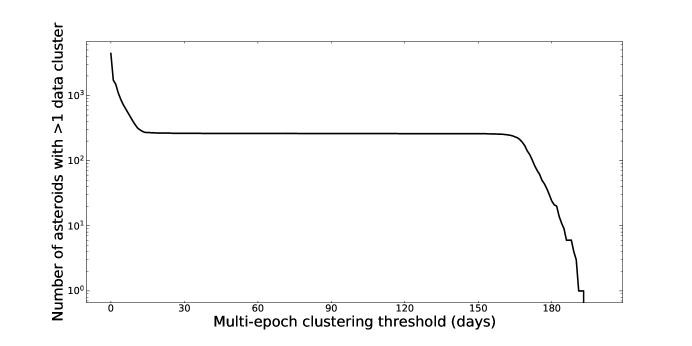
In the sixth filter, we applied a simple clustering algorithm to split the data for each asteroid into one or more subsets of observation epochs. Specifically, we split the data set whenever we found that consecutive observations were more than 30 days apart (Figure 1). As demonstrated in Figure 1, the time elapsed between observation clusters often exceeds 30 days, which is due to the interaction between the WISE observational cadence and the asteroid positions. We calculated independent solutions for each cluster in part to facilitate comparisons with results from the NEOWISE team, which presented different diameter solutions for different epochs. The separate solutions also help manage large differences in phase angle across observations.

Figure 1: Number of asteroids affected by a multi-epoch clustering threshold value of $N$ days as a function of $N$. Note that the curve flattens at a threshold value of $\sim$30 days.

Seventh, we removed any subset of data that did not include at least three remaining observations in each of the four WISE bands. The three data points are required to enable fits with three adjustable parameters in each band (Section 3.6).

Finally, we implemented a basic pre-fit outlier rejection procedure. Any observation with a flux $\geq$ 1.5 mag from the next lowest or highest flux within its cluster of observational epochs was removed. This step removed a very small number of observations and did not change the number of asteroids in the filtered data set.

After application of the data filters and outlier rejection, we were left with 82,548 observations grouped into 4685 valid clusters of observations and representing 4420 asteroids. Except for 16 asteroids that have provisional designations at the time of writing, all asteroids have received a permanent IAU number.

3 Thermal Modeling

3.1 NEATM

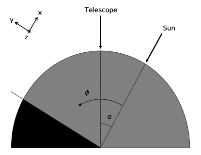
We fit the asteroid thermal data using a reparameterized version of the Near-Earth Asteroid Thermal Model (NEATM). For these calculations, we define a right-handed frame centered on the asteroid with $\vec{x}$ pointing at the Sun, $\vec{z}$ perpendicular to the plane that contains $\vec{x}$ and the observer’s line of sight, and $\vec{y}$ completing the frame (Figure 2). We then define the usual spherical coordinate system with longitude $\phi$ measured from $\vec{x}$ in the $xy$ plane and colatitude $\theta$ measured from the positive $\vec{z}$ axis. The standard version of NEATM was originally derived by Harris (1998) and gives the thermal flux of an asteroid with diameter $D$ and emissivity $\epsilon(\lambda)$ for an asteroid-observer distance $r_{\rm ao}$ and phase angle $\alpha$ as

$$F_{\rm NEATM}(\alpha,\lambda)=\frac{\epsilon(\lambda)D^{2}}{4{r_{\rm ao}}^{2}}\int_{\theta=0}^{\theta=\pi}\int_{\phi=\alpha-\pi/2}^{\phi=\alpha+\pi/2}B(\lambda,T(\theta,\phi))\sin^{2}\theta\cos(\phi-\alpha)\,d\phi\,d\theta,$$ (1)

where $B(\lambda,T)$ is the Planck distribution given by

$$B(\lambda,T)=\frac{2hc^{2}}{\lambda^{5}}\frac{1}{\exp(\frac{hc}{\lambda kT})-1},$$ (2)

and $T(\theta,\phi)$ is the temperature distribution given by

$$T(\theta,\phi)=T_{\rm ss}\max{(0,\sin\theta\cos\phi)}^{1/4},$$ (3)

where $T_{\rm ss}$ is the sub-solar temperature. In these expressions, $\lambda$ is the wavelength, $h$ is Planck’s constant, $k$ is Boltzmann’s constant, and $c$ is the speed of light. The integration domain includes the hemisphere visible to the observer with all nightside ($|\phi|>\pi/2$) emission set to zero through equation (3). The prescription for zero emission on the nightside is a feature of NEATM. Appendix A describes an equivalent NEATM formulation with a different choice of angles.

Figure 2: Definition of coordinate frame for NEATM calculations. Both the Sun and telescope are in the plane of the page. The spin vector is not shown.

The sub-solar temperature $T_{\rm ss}$ is given by

$$T_{\rm ss}=\left(\frac{S_{0}(1-A)}{\epsilon\sigma\eta{r_{\rm as}}^{2}}\right)^{1/4}.$$ (4)

where $S_{0}=1360.8$ W/m² is the solar constant, $A$ is the Bond albedo, $\sigma$ is the Stefan-Boltzmann constant, $r_{\rm as}$ is the asteroid-Sun distance, and $\eta$ is a free parameter in NEATM referred to as the “beaming parameter”. The Bond albedo is typically approximated as the visible-band Bond albedo (Hapke, 2012)

$$A\approx A_{V}=p_{\rm V}q,$$ (5)

where $p_{\rm V}$ is the visible-band geometric albedo and $q$ is the visible-band phase integral, which is typically obtained by integrating the empirical asteroid phase function $\psi_{\rm HG}(\alpha,G)$ (Bowell et al., 1989). Integration of $\psi_{\rm HG}$ over all phase angles gives $q$ as

$$q=0.285596+0.656288\times G,$$ (6)

which is different from the frequently used but incorrect expression described by Bowell et al. (1989):

$$q=0.290+0.684\times G.$$ (7)

For a typical value of the slope parameter G=0.15, the two expressions differ by 2%.

Myhrvold (2018a) pointed out that two of the fitting parameters in the traditional NEATM, $p_{\rm V}$ and $\eta$, appear in the numerator and denominator of Equation (4), thereby increasing the likelihood of numerical instabilities or convergence to local minima. To remedy this issue, Myhrvold (2018a) proposed a reparameterized version of NEATM, which introduced a new fitting parameter, the pseudo-temperature $T_{1}$:

$$T_{1}=\left(\frac{S_{0}(1-A)}{\epsilon\sigma\eta}\right)^{1/4}.$$ (8)

This parameter has the physical interpretation of $T_{1}=T_{\rm ss}$ at $r_{\rm as}=1$. With this reparameterization, equation (4) becomes

$$T_{\rm ss}=\frac{T_{1}}{\sqrt{r_{\rm as}}}.$$ (9)

When fitting thermal flux with the reparameterized version of NEATM to asteroid data, the only floating parameters are $T_{1}$, which controls the shape of the curve, and the asteroid diameter $D$, which controls the amplitude of the curve. Importantly, the reparameterization highlights the fact that there are only two, not three, degrees of freedom in this problem (Myhrvold, 2018a). We emphasize that fitting thermal flux does not rely in any way on the absolute visual magnitude $H$ of the asteroid.

3.2 Reflected Sunlight

Because WISE observations of asteroids are sensitive to reflected sunlight, we add a reflected flux component to the model

$$F_{\rm REFL}(\alpha,\lambda)=p(\lambda)\frac{D^{2}}{4{r_{\rm ao}}^{2}}\psi_{\rm HG}(\alpha,G)F_{\rm Sun}(\lambda),$$ (10)

where $p(\lambda)$ is the geometric albedo and $F_{\rm Sun}(\lambda)$ is the solar flux incident on the asteroid. The solar flux is often estimated with a blackbody model at 5778 K

$$F_{\rm Sun,\rm BB}(\lambda)=\frac{\pi{R_{\rm Sun}}^{2}}{{r_{\rm as}}^{2}}B(\lambda,5778\,{\rm K}),$$ (11)

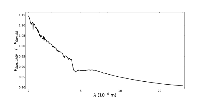
where $R_{\rm Sun}$ is the solar radius. However, the true solar spectrum deviates by up to 20% from the blackbody model at near-infrared wavelengths (Figure 3). In order to provide the best possible model of reflected light, we used an actual solar spectrum obtained with satellite measurements. Specifically, we used the 2010 yearly averaged solar spectrum from the Solar Radiation and Climate Experiment (SORCE) compiled by the University of Colorado’s Laboratory for Atmospheric and Space Physics (LASP) and the Naval Research Laboratory (Coddington et al., 2016), i.e., we set $F_{\rm Sun}=F_{\rm Sun,\rm LASP}$.

Figure 3: Ratio of the 2010 yearly averaged solar flux from satellite measurements to the flux of a blackbody at 5778 K. Deviations of up to 20% occur at WISE operating wavelengths.

3.3 Integration over WISE Bands

The total flux we expect to observe from a given asteroid is the sum of the emitted and reflected components:

$$F_{\rm total}(\alpha,\lambda)=F_{\rm NEATM}(\alpha,\lambda)+F_{\rm REFL}(\alpha,\lambda).$$ (12)

Equation 12 gives the total model flux at a single wavelength. However, the WISE bands span bandwidths on the order of $\sim 2-10$ microns (e.g., Wright et al., 2010, Figures 6 and 7). In order to determine the flux measured by the receiver, we integrate Equation 12 over the receiver response:

$$\langle F_{\rm total}\rangle=\frac{\int\lambda R(\lambda)F_{\rm total}(\alpha,\lambda)\,d\lambda}{\int\lambda R(\lambda)\,d\lambda},$$ (13)

where $R(\lambda)$ is the relative spectral response (RSR) of the WISE sensors, measured in terms of quantum efficiency per photon. A separate integration is performed for each WISE band W_i. When integrating over the W4 RSR, we scaled the wavelengths by a factor of 1.033 as recommended by Brown et al. (2014), who found that this correction reduced the residual between the measured W4 photometry and the photometry synthesised from spectra of galaxies and planetary nebulae.

In order to avoid redundant computations when fitting thousands of models, we calculated Equation 13 for a fine grid of $T_{\rm ss}$ and $\alpha$ values, with the integrand of Equation 1 as the model flux. This allowed us to replace the computationally expensive integrations with efficient table lookups and bilinear interpolations between table entries, which considerably reduced the processing time. In the most relevant temperature range of $T_{\rm ss}=200-400$K, the fractional errors introduced by the table lookup procedure are $<$1 ppm. The worst possible fractional errors occur for extremely low temperatures, $T_{\rm ss}=20$K, and remain $<$0.5%.

Before comparing the model flux to the observations, we converted the calculated flux to units of magnitude in order to match the flux reported by WISE:

$$F_{\rm model}=-2.5\,\log_{10}\langle F_{\rm total}\rangle.$$ (14)

3.4 Implementation of Kirchhoff’s Law

Emissivity and albedo are related through Kirchhoff’s law of thermal radiation, which can be expressed as follows:

$$p(\lambda)=\frac{1-\epsilon(\lambda)}{q}.$$ (15)

When fitting WISE data, we allowed for one $\epsilon(\lambda)$ value per WISE band, such that

$$\epsilon(\lambda)=\begin{cases}\epsilon_{1},&\lambda\in W1\\ \epsilon_{2},&\lambda\in W2\\ \epsilon_{3},&\lambda\in W3\\ \epsilon_{4},&\lambda\in W4\end{cases}$$ (16)

Because W3 and W4 are dominated by thermally emitted light, the emissivities for those bands are typically set (somewhat arbitrarily) by some investigators to $\epsilon_{3}=\epsilon_{4}=0.9$ during fitting. This choice is reasonable for many asteroids and has widely been used in past studies. However, other values in the range $\sim 0.5<\epsilon_{i}<1$ are physically reasonable both for likely asteroid minerals and surface conditions. We allow for this possibility with a regularized modeling approach (Section 3.6). We found that relaxing the arbitrary constraints on emissivities was important in order to obtain satisfactory fits to the data.

3.5 Least-Squares Model Fits

During the fitting procedure, we compared the model flux to the observed flux $F_{\rm obs}$ and adjusted model parameters to minimize an error term $L$. A common approach is to minimize the chi-squared error $L=\chi^{2}$ using a least-squares fitting routine. The $\chi^{2}$ error is calculated as

$$\chi^{2}=\sum_{i}\left(\frac{F_{{\rm obs},i}-F_{{\rm model},i}}{\sigma_{i}}\right)^{2},$$ (17)

where the indices $i$ represent individual data points for a given asteroid and $\sigma_{i}$ is the measurement error for the $i^{th}$ observation. The summation in Equation 17 is performed over all observations from all WISE bands within a subset of observation epochs as defined in Section 2.

The chi-squared minimization is common in asteroid thermal modeling, but it is problematic with WISE data because the observation error estimates produced by the WISE pipeline are problematic (Hanuš et al., 2015; Myhrvold, 2018a, b). It is also problematic with the NEATM model, which relies on the assumption of spherical asteroids. In a rigorous chi-squared implementation, the error term in Equation (17) must include modeling error, e.g., deviations from a constant surface area due to nonspherical asteroid shapes. Using a chi-squared approach with incorrect error values can trap the solution in false minima (Ratkowsky, 1983).

3.6 Regularized Model Fits

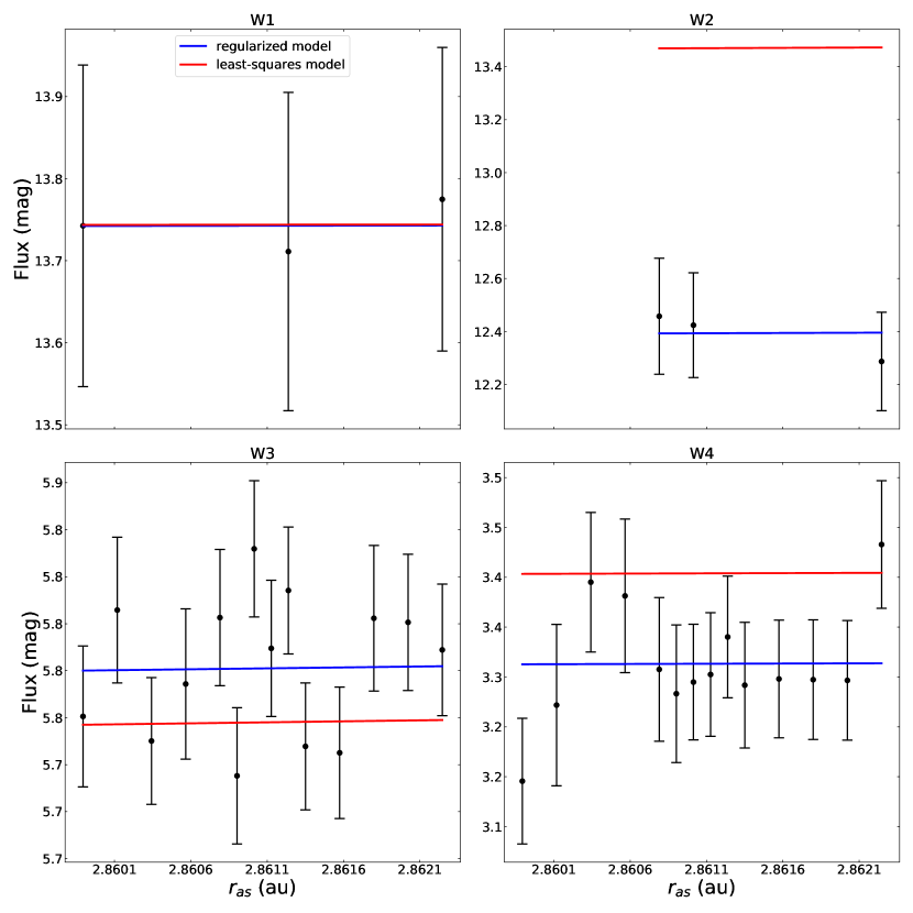
Myhrvold (2018b) first demonstrated that model fits performed as described in Section 3.5 can result in poor fits to the data (see his Figure 3). Specifically, he showed that many (up to 50%) NEOWISE model fits miss the data completely in one or more WISE bands. In a withdrawn manuscript, Wright et al. (2018) ascribed the problem of fits missing the data in the case of two asteroids to a previously unreported software bug in the NEOWISE modeling code that was identified and fixed in 2011. This bug potentially corrupts all NEOWISE model estimates obtained prior to the bug fix. While the bug may explain the problem with reported NEOWISE results for these two asteroids, the problem of model fits missing data is widespread and points to a more fundamental issue. Indeed, a cursory analysis suggests that at least $\sim 1600$ asteroids out of 4420 ($\sim 36\%$) in our sample exhibit least-squares model fits with unacceptably low quality. We obtained this number by counting the number of asteroids that, in at least one of the bands, have a residual larger than the measured error for every point, and the residuals in that band are either all positive or all negative. Figure 4 shows an example.

Figure 4: Best-fit models to 38 observations of asteroid 7451 Verbitskaya with the standard NEATM (least-squares model) and our regularized approach (regularized model). Flux values shown in this figure are displayed as a function of asteroid-Sun distance and reduced to the values that would be observed at an asteroid-observer distance $r_{\rm ao}$ = 1 au. The least-squares model completely misses the data in W2, and the miss is not due to the small number of points in W2 because the least-squares model fits the data well in W1 with the same number of points. In addition, the small number of points in W2 does not prevent the regularized model from fitting the data. The $\chi^{2}$ values are 152 (least-squares model) and 25 (regularized model) whereas the sums of squares of (unweighted) residuals are 3.7 (least-squares model) and 0.075 (regularized model).

We found that the quality of the model fits can be improved by relaxing the restrictions placed on the per-band emissivity values $\epsilon_{i}$, which are arbitrarily set to 0.9 in the NEOWISE solutions. Specifically, we allowed all four values to vary in the range $0<\epsilon_{i}<1$, although results rarely yield $\epsilon_{i}<0.7$. However, the additional degrees of freedom introduced with varying emissivities are not handled well by conventional least-squares curve fitting. Therefore, we used a regularized method and reined in the additional freedom in the model with a regularization term that helps satisfy two objectives. First, we wish to favor models with high emissivity values. Second, we wish to disfavor models with a large dispersion in emissivity values. Both of these objectives are aligned with the classic $\epsilon=0.9$ assumption across all bands and with observational data (e.g., Figure 1 of Myhrvold, 2018a). Laboratory spectra from meteorites and previous work on IR spectra of asteroids indicate that asteroid materials generally have emissivity values that are close to unity and do not exhibit substantial wavelength dependence (Supplementary Material of Myhrvold, 2018a, and references therein).

The regularized model loss is given by the sum of a classic loss function and a regularization term:

$$L=L_{\rm data}+R_{\rm model}.$$ (18)

In order to assign approximately equal weights to the classic loss function and the regularization term, we normalized each one to a value near unity with the following expressions. The scaled residual loss $L_{\rm data}$ is given by

$$L_{\rm data}=\frac{L_{2}-L_{\rm min}}{L_{\rm min}},$$ (19)

where $L_{2}$ is the sum of squares of (unweighted) residuals, $L_{2}=\sum\limits_{i}(F_{\rm obs,i}-F_{\rm model,i})^{2}$, and $L_{\rm min}$ is a lower bound on $L_{2}$, which we obtained by fitting the model (Equation 12) to each individual band W1–W4 with three floating parameters ($T_{1}$, $D$, and $\epsilon_{i}$), then summing the sums of squares of residuals over all four bands. We chose $L_{2}$ instead of $\chi^{2}$ because of the problems associated with the $\chi^{2}$ metric described in Section 3.5.

The scaled regularization loss is given by

$$R_{\rm model}=||\epsilon-0.9||.$$ (20)

where $||\vec{a}||=\left[\sum_{i}a_{i}^{2}\right]^{0.5}$ is the norm operator and $\epsilon$ is the emissivity vector $\{\epsilon_{1},\epsilon_{2},\epsilon_{3},\epsilon_{4}\}$. We also obtained fits with a few other forms of the regularization loss (Appendix B), which confirmed the robustness of our general conclusions but did not perform quite as well in terms of diameter accuracy.

We used the Limited-memory Broyden–Fletcher–Goldfarb–Shanno algorithm with Box constraints (L–BFGS–B; Byrd et al., 1995) to minimize the loss $L$ for every set of observations. We executed the fitting routine seven times per asteroid with seven different initial values for $\epsilon_{1}=\epsilon_{2}=\epsilon_{3}=\epsilon_{4}$ selected from the set $\{0.6,0.7,0.8,0.85,0.9,0.95,0.99\}$. In some cases, we detected a loss $L_{2}$ during the fit that was lower than our initial estimate of $L_{\rm min}$. When this situation arose, we updated the value of $L_{\rm min}$ accordingly and restarted the fitting procedure.

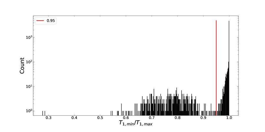
After applying this procedure, we noticed that, in approximately 8% of the cases, the seven solutions to our fitting procedure did not have a single minimum but rather fell into one of two local minima. One of the minima occurs at $T_{1}\sim 230-380$ K with a comparatively larger diameter $D$, whereas the other minimum occurs at a larger value of $T_{1}$ $\sim 330-430$ K but smaller diameter $D$ (Figure 5). Because the $T_{1}$ parameter has the physical interpretation of subsolar temperature, i.e., $T_{1}=T_{\rm ss}$ at $r_{\rm as}=1$ (Equation 8), we expect most thermal model fits to have $T_{1}=350-450$ K. Thus, when two groups of local minima were detected, we chose to report the best-fit solution among the high-$T_{1}$ group. Specifically, we selected all solutions with $T_{1}\geq 95$% of the largest $T_{1}$ in any given fit, and then selected the best-fit solution (smallest $L$) amongst those.

Figure 5: Ratio of the largest and smallest $T_{1}$ values amongst the seven solutions to our fitting procedure. For ratios below 0.95, the fits fall into one of two local minima. We report the best-fit solution from the high-$T_{1}$ group.

3.7 Bootstrap Trials

Because the WISE uncertainties are in doubt (Hanuš et al., 2015; Myhrvold, 2018b) and do not include lightcurve errors, we turned instead to the Bootstrap method to estimate errors in diameter and other parameters(e.g., Feigelson & Babu, 2012; Ivezić et al., 2014). We performed 200 bootstrap trials for every asteroid in order to reduce the influence of any remaining data outliers and to obtain an estimate of the uncertainty on the model fit parameters. For each trial, we randomly sampled the asteroid data with replacement until the number of samples matched the original number of samples. We repeated the sampling procedure as necessary until the requirement of at least 3 data points in each of the four WISE bands was met. We then performed a model fit (Section 3.6) on the sampled data. We repeated this process 200 times per asteroid to obtain 200 unique model fits. The final model parameters as well as their uncertainties were obtained by taking the mean value and the standard deviations of the 200 bootstrap fits, respectively.

4 Results

4.1 Diameters

We present 4685 thermal model fit results for a total of 4420 asteroids (4326 MBAs and 94 NEAs). The full table of results is available online. A sample of the table is shown in Table 2.

Table 2: Results of thermal model fits showing the asteroid number or provisional designation, the unique 7+ digit Spacecraft and Planet Kernel (SPK) ID of the Navigation and Ancillary Information Facility (NAIF) node of the NASA Planetary Data System, the mean observation date of each cluster of observational epochs and the number of data points for the subset of observations used in the fit, and best-fit estimates and errors of the diameter $D$, pseudo-temperature $T_{1}$, emissivities $\epsilon_{i}$, and geometric albedo $p_{\rm V}$. Parameter uncertainties (1$\sigma$) are obtained by calculating the standard deviations of 200 bootstrap resampling solutions. Albedo values are calculated on the basis of $H$ values reported by HORIZONS, and the corresponding error values are obtained by assuming an uncertainty of 0.25 mag on the $H$ values (Vereš et al., 2015, Figure 5). The values $p_{\rm V}^{\prime}$ and $\sigma_{p_{\rm V}^{\prime}}$ represent the albedo and its error calculated using $H$ values from Vereš et al. (2015) when available (defaulting to the HORIZONS $H$ values otherwise). (This table is available in its entirety in a machine-readable form in the online journal. A portion is shown here for guidance regarding its form and content.

Object	SPK ID	Mean MJD	$N$	$D$ (km)	$\sigma_{D}$	$T_{1}$	$\sigma_{T_{1}}$	$\epsilon_{1}$	$\sigma_{\epsilon_{1}}$	$\epsilon_{2}$	$\sigma_{\epsilon_{2}}$	$\epsilon_{3}$	$\sigma_{\epsilon_{3}}$	$\epsilon_{4}$	$\sigma_{\epsilon_{4}}$	$p_{\rm V}$	$\sigma_{p_{\rm V}}$	$p_{\rm V}^{\prime}$	$\sigma_{p_{\rm V}^{\prime}}$
131	2000131	55322.809852	60	30.59	0.6	405.15	2.6	0.899	0.005	0.897	0.003	0.859	0.037	0.926	0.022	0.194	0.045	0.153	0.036
155	2000155	55395.529229	53	44.65	2.6	379.44	9.9	0.981	0.002	0.939	0.013	0.890	0.037	0.918	0.026	0.029	0.007	0.023	0.006
170	2000170	55404.853180	42	35.42	1.8	389.20	8.2	0.856	0.012	0.861	0.018	0.849	0.018	0.917	0.014	0.256	0.065	0.202	0.051
180	2000180	55319.783820	43	24.79	2.2	396.42	14.7	0.861	0.026	0.867	0.028	0.896	0.029	0.913	0.039	0.239	0.070	0.188	0.055
183	2000183	55234.369656	64	30.73	2.9	412.37	15.6	0.842	0.028	0.909	0.023	0.867	0.091	0.947	0.055	0.278	0.082	0.219	0.065
183	2000183	55398.940284	40	30.76	5.2	405.50	29.0	0.850	0.053	0.887	0.029	0.862	0.094	0.944	0.054	0.277	0.114	0.218	0.090
193	2000193	55250.762781	33	28.82	2.7	374.72	16.2	0.891	0.022	0.913	0.018	0.895	0.035	0.908	0.029	0.249	0.073	0.196	0.058
214	2000214	55246.883604	41	29.72	7.1	372.48	88.5	0.808	0.143	0.692	0.300	0.841	0.195	0.863	0.064	0.388	0.205	0.306	0.162
239	2000239	55368.131442	44	42.88	2.8	391.03	12.5	0.968	0.005	0.955	0.011	0.902	0.025	0.907	0.020	0.060	0.016	0.047	0.013
242	2000242	55408.924526	49	46.76	3.1	353.12	13.1	0.914	0.014	0.901	0.014	0.891	0.031	0.907	0.018	0.144	0.038	0.114	0.030
244	2000244	55208.721440	39	10.93	0.5	393.35	5.6	0.848	0.015	0.901	0.002	0.853	0.040	0.920	0.025	0.226	0.056	0.178	0.044
251	2000251	55351.026065	86	33.80	3.4	367.85	19.5	0.887	0.027	0.867	0.014	0.878	0.057	0.904	0.034	0.163	0.050	0.129	0.039
254	2000254	55307.007853	60	12.41	0.5	384.11	5.5	0.832	0.018	0.898	0.003	0.847	0.034	0.918	0.019	0.227	0.055	0.178	0.043
262	2000262	55325.475207	39	15.17	0.1	408.46	1.2	0.828	0.004	0.880	0.002	0.823	0.009	0.929	0.005	0.225	0.052	0.177	0.041
272	2000272	55308.896108	34	36.53	2.5	331.60	10.2	0.953	0.008	0.915	0.012	0.887	0.036	0.913	0.017	0.071	0.019	0.056	0.015

To help validate our results, we compared the diameter values obtained with our model fits to a compilation of occultation diameters submitted to the Planetary Data System (PDS) (Herald et al., 2019). For this comparison (Figure 6), we used only measurements with the highest occultation quality code values of 2 or 3. When two dimensions were reported (ellipse major and minor axes $2a$ and $2b$), we calculated the diameter of a sphere with the equivalent volume, specifically $D_{\rm occ}=2(a^{2}\times b)^{1/3}$, because the orientation of the body at the time of the WISE observations cannot be assumed to be identical to the orientation at the time of the occultation observations.

Figure 6: Comparison of diameter estimates from stellar occultation observations to the results presented in this work. Herald et al. (2019) did not report uncertainties for the data points without vertical error bars. The agreement between the two data sets is quantified by a mean normalized orthogonal distance metric $\langle d_{\perp}\rangle$ of 1.1645 (see text). Asteroid 874 has a stellar occultation diameter of 51.21 $\pm$ 30.9 km and is not plotted but is included in the $\langle d_{\perp}\rangle$ calculation.

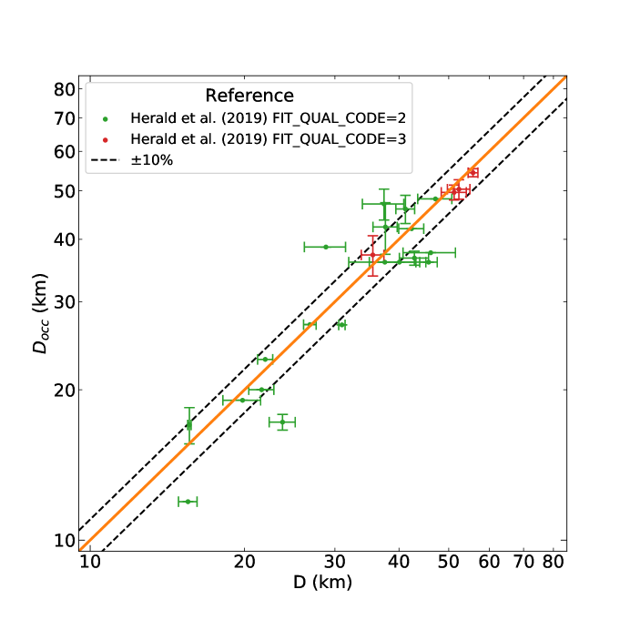
We quantified the agreement between the two data sets by calculating a mean normalized orthogonal distance metric $\langle d_{\perp}\rangle$:

$$\langle d_{\perp}\rangle=\frac{1}{N}\sum_{i=1}^{N}\frac{|D_{{\rm occ},i}-D_{i}|}{\sqrt{{\sigma_{{\rm occ},i}}^{2}+\sigma_{i}^{2}}},$$ (21)

where the summation is carried out over all $N$ comparisons, $D_{{\rm occ},i}$ and $\sigma_{{\rm occ},i}$ are the reported occultation diameters and errors, respectively, and $D_{i}$ and $\sigma_{i}$ are the diameters and errors obtained in this work. Some occultation-based diameters were reported without associated uncertainties. In these situations, we assigned the median uncertainty associated with the other occultation diameters in the comparison set ($\sim 2$ km). We found a value of $\langle d_{\perp}\rangle=1.1645\ (N=24)$ when comparing our results to the stellar occultation results, which indicates good agreement.

Note that diameter comparisons for large asteroids are not available to us because WISE observations of large asteroids are generally saturated in W3, and sometimes also in W4. In this study, we focused on the best data and rejected WISE observations reported with a nonzero saturation flag as potentially unreliable. The NEOWISE team took a different approach. They applied a linear correction to saturated W3 observations (Mainzer et al., 2011b; Masiero et al., 2011). The analytical expression for this correction was not published until a withdrawn manuscript by Wright et al. (2018), but the method for determining the coefficients in this expression was not described. In a conference paper, Wright (2019) examined a very similar linear correction term for W3 by requiring that NEOWISE model estimates match known diameters for about a hundred large asteroids. However, it is not stated whether the methodology is the same as that used in the earlier NEOWISE papers. If the known asteroid diameters were used to calibrate the linear correction, then one obviously could not use modeling results from the corrected examples to evaluate NEOWISE modeling accuracy. However there is a larger problem with the concept of applying a correction to saturated observations: very few of the asteroids observed by WISE have saturated W3 observations. Out of about 1.4 million W3 observations that meet the filter criteria of this work (except for the saturation filter), only 658 observations of 132 asteroids are identified by the WISE pipeline as saturated in W3. So even if a W3 saturation correction were to be valid, it would not be widely applicable.

We also quantified the agreement between stellar occultation diameters and the 4-band fit solutions posted by the NEOWISE team to the PDS (Mainzer et al., 2019). We used the set of 19 asteroids that are common to NEOWISE, our solutions, and the solutions of Herald et al. (2019). We found values of $\langle d_{\perp,{\rm this\ work}}\rangle=1.247\ (N=19)$ and $\langle d_{\perp,{\rm NEOWISE}}\rangle=2.336\ (N=19)$ when comparing the thermal fit results to the stellar occultation results. This metric suggests that our results more closely match stellar occultation results than the NEOWISE results, by a factor of approximately 2 in this metric. Some of this difference is related to differences in diameter uncertainties and the fact that the bootstrap method provides more realistic uncertainties than the formal errors of least-squares fits.

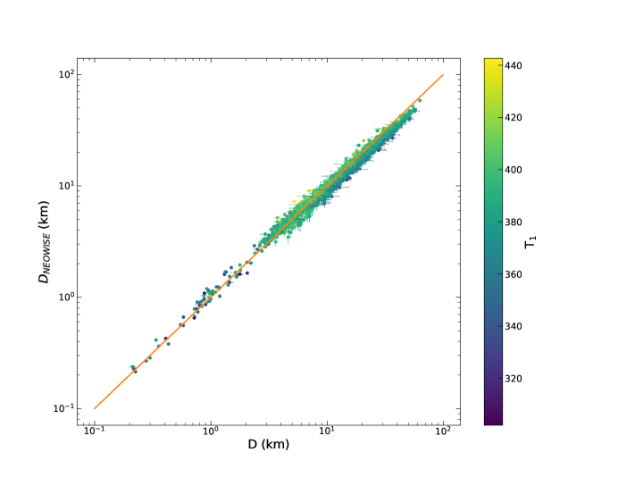
We also compared our diameter results and associated uncertainties directly to the results posted to the PDS by the NEOWISE team (Mainzer et al., 2019). A total of 2789 model fits of 2651 unique asteroids (2,580 MBAs and 71 NEAs) were common between the NEOWISE results and our results. Although the diameter comparisons are generally favorable (Figure 7), there are notable differences. Some of the diameter discrepancies for some of the asteroids are likely related to a software bug that, according to Wright et al. (2018), was discovered and fixed in 2011 and affected more than 100,000 NEOWISE diameter estimates published in 2011. Inspection of the diameter values affected by the bug indicates that they have not been corrected in the latest NEOWISE PDS release (Mainzer et al., 2019). Other sources of discrepancies are related to data selection and model differences (Sections 2 and 3). We also found that the NEOWISE estimates of diameter uncertainties are generally 3 times smaller than the bootstrap error estimates. This finding suggests that NEOWISE diameter uncertainties may be based on the incorrect per-observation uncertainties from the WISE pipeline (Hanuš et al., 2015; Myhrvold, 2018a, b) as well as on the formal uncertainties of least-squares fits, which generally under-estimate actual uncertainties.

Figure 7: Comparison of 2789 NEOWISE 4-band diameter results to the results presented in this work. The best-fit $T_{1}$ parameter is shown with a color scale. The apparent horizontal structure is related to the fact that NEOWISE diameter uncertainties are generally $\sim$3 times smaller than the more realistic bootstrap uncertainties used in this work.

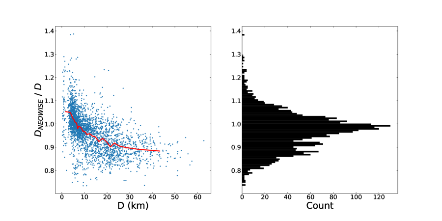
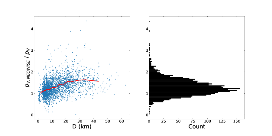
Finally, we computed the ratio of the 4-band NEOWISE diameter values to those presented in this work. Despite considerable scatter, a size-dependent bias is detectable (Figure 8). The size-dependent bias could in principle be attributed to the NEOWISE data analysis, our data analysis, or both. However, because our results more closely match the independent size calibration provided by occultation diameter estimates, we believe that the size-dependent bias is attributable to the NEOWISE data-processing pipeline, which relies on the assumption of emissivities of 0.9 in all bands. The fractions of asteroids whose NEOWISE diameter estimates are in agreement with our results within $\pm 5\%$, $\pm 10\%$, $\pm 15\%$, and $\pm 20\%$ are 48.7%, 74.4%, 90.5%, and 97.9%, respectively. The largest differences are $\pm 30\%$.

If we assume that the occultation diameter estimates are exact, we find that infrared diameter estimates in the comparison sample have a median error of 9.3% and a maximum error of 37.7%. This comparison calibrates the oft-stated claim that 4-band NEOWISE diameters are accurate to 10% – the statement appears to be correct in the best-case scenario of a carefully curated four-band data set with the techniques described in this work. However, the statement does not appear to be correct in general, as evidenced by the fact that only 74% of NEOWISE four-band diameters agree with ours to $\pm$10%. In a planetary defense context, a 9.3% error in diameter corresponds to a 28% error in mass and impact energy. With a size-dependent bias that overestimates the diameters of possible impactors, i.e., asteroids smaller than 5 km, the consequences of the impact hazard calculated with 4-band NEOWISE diameter estimates may be slightly exaggerated.

Figure 8: Distribution of NEOWISE 4-band diameters divided by the corresponding diameters obtained in this work. The red solid line shows the mean ratio obtained in consecutive diameter bins each containing 100 values. Approximately 98% of the 2651 asteroids among our carefully curated sample of 4420 asteroids have NEOWISE diameter values that agree with ours within $\pm$20%.

4.2 Albedos

We calculated geometric albedo $p_{\rm V}$ values for all asteroids with known absolute magnitude $H$ values from HORIZONS as well as the definition for visible-band geometric albedo $p_{\rm V}$:

$$p_{\rm V}\equiv\left(\frac{1329}{D}\right)^{2}\,10^{-\frac{2H}{5}},$$ (22)

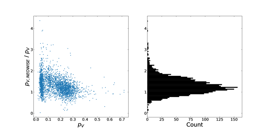
where $D$ is the diameter in km (Harris & Lagerros, 2002). We performed this calculation with two sets of $H$ values. First, we used the $H$ values obtained from HORIZONS (Table 2). Second, we used the $H$ values reported by Vereš et al. (2015) if available, otherwise the $H$ values obtained from HORIZONS augmented by 0.26 to account for the mean systematic offset reported by Vereš et al. (2015). Comparisons of the H_HORIZONS-based albedo values to those reported by the NEOWISE team (Mainzer et al., 2019) are shown in Figures 9 and 10.

Figure 9: Comparison of 2,971 NEOWISE visible albedo results to the results presented in this work. In this comparison, HORIZONS values of $H$ were used in the calculation of $p_{\rm V}$. Asteroid 2010 MA113, which does not have a NEOWISE albedo estimate, is not shown.

Figure 10: Comparison of 2,788 NEOWISE visible albedo results to the results presented in this work, as a function of $D$. The red solid line shows the mean ratio obtained in consecutive diameter bins each containing 100 values. In this comparison, HORIZONS values of $H$ were used in the calculation of $p_{\rm V}$. Asteroid 2010 MA113, which does not have a NEOWISE albedo estimate, is not shown.

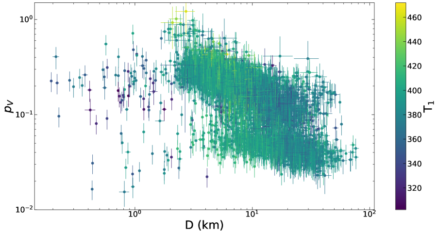
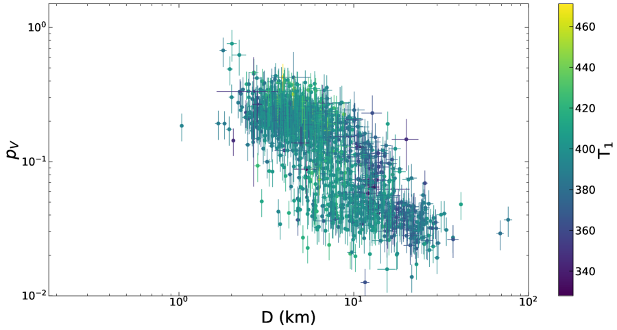
Plots of the visible albedo values as a function of asteroid diameters (Table 2) reveal at least two clusters and an apparent size-dependence of albedo in each cluster (Figure 11). The apparent size dependence persists regardless of the source of the $H$ values used in the albedo calculation. However, the apparent size dependence is likely due to a selection effect because the optical surveys and MPCORB database are not complete with respect to the smaller, darker objects. Versions of these figures with color-coding according to phase angle and the quantity $r_{\rm ao}\times r_{\rm as}$ are shown in appendix (Figure 18). They reveal the expected selection effect that objects with the smallest diameters are detected when observed at the smallest distances, which also tends to occur at the largest phase angles. Figure 19 in appendix reveals a mild correlation (correlation coefficient 0.2) between visible-band geometric albedo $p_{\rm V}$ and pseudo-temperature $T_{1}$. Figure 20 in appendix shows the distribution of phase angles.

Figure 11: Visible-band geometric albedo $p_{\rm V}$ as a function of the asteroid diameter $D$. The data are color-coded according to pseudo-temperature $T_{1}$. We assumed an uncertainty of 0.25 mag (Vereš et al., 2015, Figure 5) on the $H$ values to calculate the error bars on $p_{\rm V}$. (Top) Albedos calculated with $H$ values obtained from HORIZONS. (Bottom) Albedos calculated with $H$ values obtained from Vereš et al. (2015).

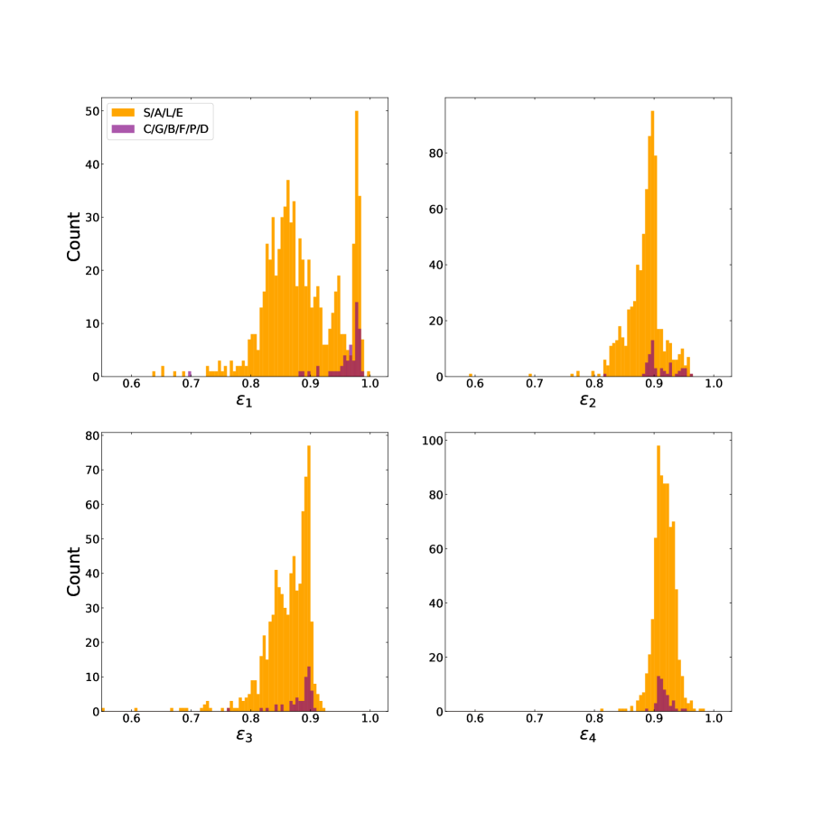
Only about 18% of asteroids in our sample have known taxonomic classes according to the latest collection available on the NASA Planetary Data System(Neese, 2010). The diameters and albedos of 791 asteroids with known taxonomic classes are shown on Figure 12. As expected, asteroids with classes traditionally thought to correspond to darker asteroids (C/G/B/F/P/D) have low albedos. However, asteroid with classes traditionally thought to correspond to lighter asteroids (S/A/L/E) have albedos that span the full range of observed values. The low-albedo asteroids in the S/A/L/E classes tend to be associated with high median infrared emissivities (Section 4.3). The “C” classification of the high-albedo asteroid 1653 Castafiore appears to be an outlier.

Figure 12: Visible-band geometric albedo $p_{\rm V}$ as a function of the asteroid diameter $D$ for 791 asteroids with known taxonomic classifications. S/A/L/E-class asteroids are split according to their median infrared emissivity (Section 4.3). Albedos were calculated with $H$ values obtained from HORIZONS.

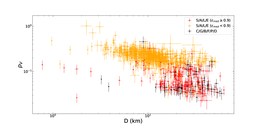
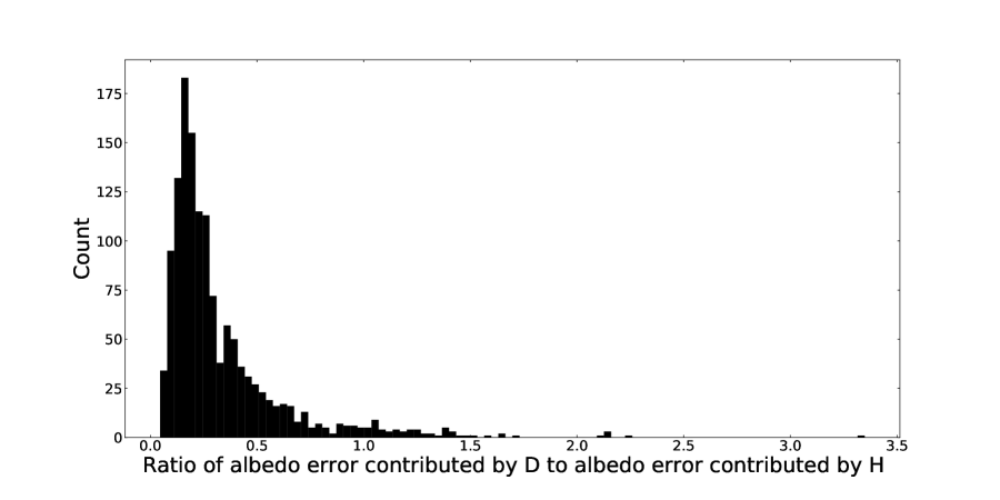
Figure 13 indicates that the errors on the visible albedo values are dominated by the uncertainty on the $H$ measurement, which we assumed to be 0.25 mag for all asteroids (Vereš et al., 2015, Figure 5). Pravec et al. (2012) described 0.2 mag as the smallest plausible uncertainty on absolute magnitudes for survey data and Masiero et al. (2021) argued that these uncertainties will likely reach up to $\sim$1 mag for objects observed at large phase angles. We found that $H$ uncertainties largely dominate the albedo error budget even with a generous assumption on the quality of $H$ values.

Figure 13: Ratio of the two terms used to calculate the visible-band geometric albedo $p_{\rm V}$ error. We assumed an uncertainty of 0.25 mag (Vereš et al., 2015, Figure 5) on the $H$ values. Errors on the diameter estimates were obtained by calculating the standard deviations of 200 bootstrap resampling solutions. Note that the error on $H$ is the dominant contribution for $>91\%$ of the asteroids.

4.3 Emissivities

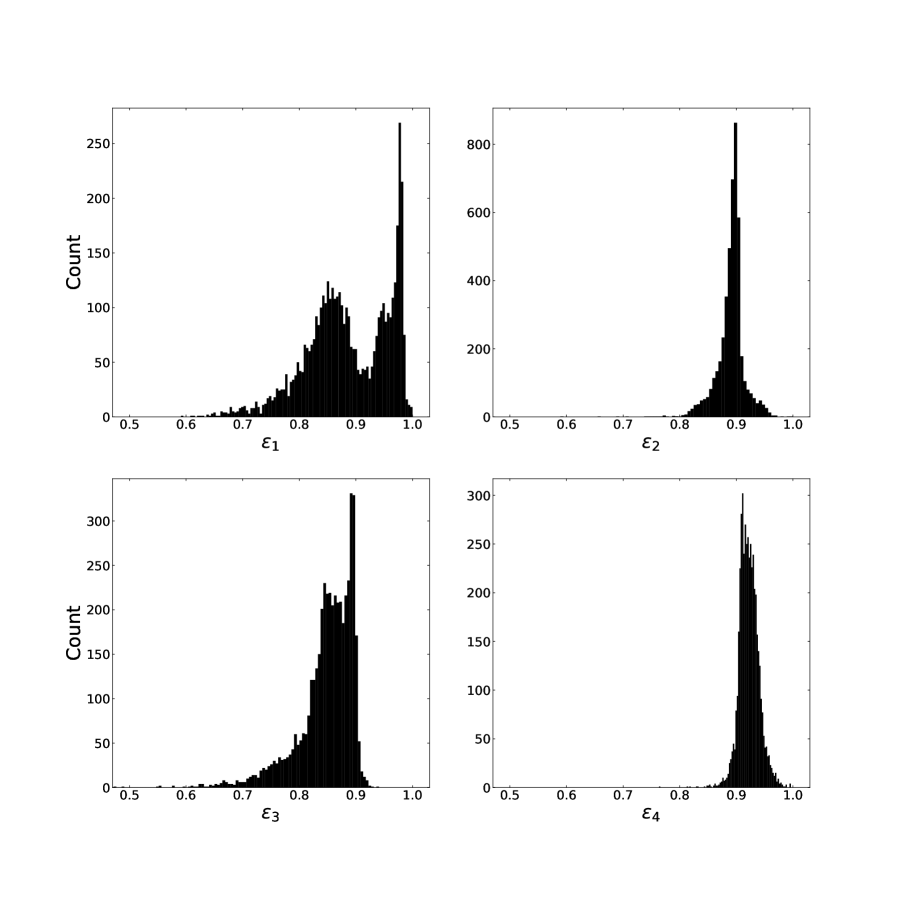
The distributions of emissivity values obtained with our asteroid thermal model fits are shown in Figure 14. Although our regularized fitting algorithm does favor small dispersions among emissivities, the correlation matrix (Table 3) indicates that there was sufficient freedom for individual emissivities to take on disparate values. The emissivity in W2 does not correlate strongly with emissivities in any other band. Band W2 behaves somewhat differently from other bands in that W2 flux includes varying contributions from emitted and reflected light depending on observing circumstances, whereas W1 flux is almost entirely due to reflected light and W3–4 fluxes are almost entirely due to thermal emission.

Figure 14: Histograms of best-fit emissivity values for each of the WISE bands for 4420 asteroids.

	$\epsilon_{1}$	$\epsilon_{2}$	$\epsilon_{3}$	$\epsilon_{4}$
$\epsilon_{1}$	1.	0.241	0.758	-0.157
$\epsilon_{2}$	0.241	1.	0.171	0.152
$\epsilon_{3}$	0.758	0.171	1.	-0.526
$\epsilon_{4}$	-0.157	0.152	-0.526	1.

Table 3: Correlation matrix of best-fit infrared emissivities for 4420 asteroids.

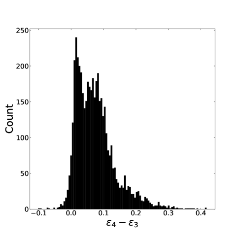
We examined the distribution of $\epsilon_{4}-\epsilon_{3}$ values (Figure 15). The distribution is asymmetric and indicates generally higher emissivity values in W4. This observation reflects differences in physical properties at these two wavelengths and is consistent with lab spectra of chondritic materials (e.g., Myhrvold, 2018a, Figure 1).

Figure 15: Histogram of $\epsilon_{4}-\epsilon_{3}$ values for 4420 asteroids.

We examined the emissivities of 791 asteroids with known taxonomic classes (Figure 16). As expected, asteroids with classes traditionally thought to correspond to darker asteroids (C/G/B/F/P/D) have high emissivity values. However, asteroid with classes traditionally thought to correspond to lighter asteroids (S/A/L/E) have emissivities that span the full range of observed values.

Figure 16: Histograms of best-fit emissivity values for each of the WISE bands for 791 asteroids with known taxonomic type.

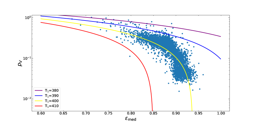
The median infrared emissivity calculated from the best-fit $\epsilon_{i}$ $(1\leq i\leq 4)$ values is highly (negatively) correlated with the visible-band geometric albedo $p_{\rm V}$, with a correlation coefficient of -0.842. The infrared emissivities and the visual albedo are connected through the assumption that the Bond albedo $A\approx A_{V}$ and equation (8), as illustrated on Figure 17. The emissivity assumptions therefore have an impact on calculated albedo values. For instance, the albedo of an asteroid with best-fit median emissivity of 0.93 would go from $\sim$2% to $\sim$10% if we forced its emissivity to 0.9. Conversely, promoting high emissivities through a regularization method may result in lower albedos. These trends may explain in part the apparent dichotomy in albedos of S/A/L/E-class asteroids observed on Figure 12.

Figure 21 in appendix reveals a mild negative correlation (correlation coefficient -0.27) between the median emissivity value and pseudo-temperature $T_{1}$.

Figure 17: Relationship between visible-band geometric albedo $p_{\rm V}$ and median infrared emissivity for 4420 asteroids. The colored curves represent equation (8) with $q=0.384$, $\eta=1$, and various values of the pseudo-temperature $T_{1}$.

4.4 Beaming Parameter

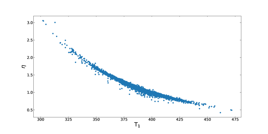
The procedure used in this work does not fit for the beaming parameter $\eta$, which has a variety of obscure physical interpretations (Myhrvold, 2018a). Instead, we absorb it into a pseudo-temperature whose physical interpretation is straightforward. For completeness and for comparison to other studies that use this parameter, we used equation (8) to estimate the value of the beaming parameter and verify its behavior as a function of pseudo-temperature $T_{1}$ (Figure 22 in Appendix).

5 Conclusions

We described the results of our analysis of 82,548 WISE observations of 4420 asteroids. In particular, we provided solutions to 131 asteroids not analyzed by the NEOWISE team and to 1,778 asteroids not analyzed with 4-band data by the NEOWISE team. The subset of asteroids was carefully curated to include at least three observations in each one of the four WISE bands and to eliminate measurements with artifacts, low S/N, poor photometric quality, saturation, or questionable PSF fits. The last two of these filters remove observations that are likely problematic but were not discarded in previous work. We also eliminated sources that were reported at large distances from the expected ephemeris positions of asteroids or that experienced conjunction or near-conjunction conditions or possible background confusion. These distance-based data filters are also novel and eliminate incorrect data that were not previously excluded according to NEOWISE descriptions. The curated set of observations provides the best possible scenario for analysis of four-band infrared data and yields useful performance benchmarks for diameter, emissivity, and albedo determinations. Observations in less favorable conditions, e.g., two-band data, are expected to yield estimates with larger errors.

We compared best-fit diameter results to independent, high-quality stellar occultation size estimates. This calibration revealed that four-band diameter estimates can be recovered with a median precision of 9.3% and a worst-case precision of 37.7% in this sample, which correspond to median and worst-case precisions of 28% and 113% on mass and impact energy.

Our results indicate that forcing emissivities to an arbitrary value of 0.9 can have detrimental effects on diameter and albedo estimates. We found that a regularized fitting algorithm with variable emissivities yields markedly better fits to the data than a least-squares fitting algorithm with emissivities arbitrarily set to 0.9. In particular, the regularized approach yields diameter estimates that are $\sim$2 times better than NEOWISE estimates, as quantified by an orthogonal distance metric with respect to high-quality stellar occultation diameter estimates. This result and others are robust with respect to four different forms of the regularization loss. The regularized approach also solved the problem of thermal fits that completely miss the data in at least one band in a substantial fraction ($\sim$36%) of asteroids. Moeyens et al. (2020) reached a similar conclusion by fitting thermal models that allowed for different emissivities within a Bayesian framework. Specifically, for a slightly different set of WISE data with different input filters, Moeyens et al. (2020) also concluded that the data supported emissivity values other than 0.9 for W3 and W4.

Our results suggest that NEOWISE estimates of diameters and albedos are affected by size-dependent biases that may pollute estimates of asteroid size distributions and slightly inflate impact hazard risk calculations.

We found that emissivities in the W3 and W4 thermal bands are imperfectly correlated ($\sim$0.53), with a marked asymmetry revealing generally higher values in W4, consistent with laboratory spectra for chondritic materials (e.g., Myhrvold, 2018a, Figure 1).

We quantified the sources of error in albedo estimates and found that the primary source of error lies in the determination of the absolute visual magnitude for over 90% of asteroids in this sample. Because albedo estimates could be readily improved with better estimates of absolute visual magnitudes, efforts similar to those of Pravec et al. (2012) and Vereš et al. (2015) are quite valuable.

Appendix A Alternate NEATM geometry

In some NEATM formulations, a left-handed coordinate system is used where $\vec{y}$ points at the Sun. Integration appears to be carried out over all latitudes and illuminated longitudes, although the portion of the hemisphere that is not visible to the observer is removed. In this formulation, it appears that the observer is confined to the $yz$ plane if $\theta$ is defined as a latitude and the $xz$ plane if $\theta$ is defined as a longitude. We can reproduce this setup with the following substitutions: $\theta\leftarrow\phi$ and $\phi\leftarrow 90^{\circ}-\theta$. The resulting expression is

$$F_{\rm NEATM}(\alpha,\lambda)=\frac{\epsilon(\lambda)D^{2}}{4{r_{\rm ao}}^{2}}\int_{\phi=-\pi/2}^{\phi=\pi/2}\int_{\theta=-\pi/2}^{\theta=\pi/2}B(\lambda,T(\theta,\phi))\cos^{2}\phi\cos(\theta-\alpha)d\theta d\phi,$$ (A1)

where the portion of the hemisphere not visible to the observer is given zero flux with

$$\begin{cases}T(\theta,\phi)=T_{\rm ss}(\cos\phi\cos\theta)^{1/4},&\text{if }\alpha-\pi/2\leq\theta\leq\alpha+\pi/2\\ 0,&\text{otherwise}\end{cases}$$ (A2)

Both formulations yield identical thermal flux values for a given set of input parameters.

Appendix B Alternate forms of the regularization loss

In the course of our investigation, we attempted a few forms of the regularization loss (Equation 20). In some formulations, we targeted a norm for the emissivity vector that corresponds to $\epsilon\sim 0.9$ or $\epsilon\sim 1$ while minimizing the dispersion between emissivity values with a second term $\sigma_{\epsilon}$, which is the standard deviation among the emissivity values:

$$R_{\rm model}=\frac{2-||\epsilon||}{2}+2\sigma_{\epsilon}.$$ (B1)

$$R_{\rm model}=\frac{1.8-||\epsilon||}{1.8}+2\sigma_{\epsilon}.$$ (B2)

$$R_{\rm model}=||\epsilon-0.9||+2\sigma_{\epsilon}$$ (B3)

Although we observed slight differences in the diameter and $T_{1}$ estimates for various versions of the regularization loss, all forms confirmed our general conclusions. In particular, all forms exhibited a bimodal distribution of $T_{\rm 1,min}/T_{\rm 1,max}$ (Figure 5) and yielded better agreement with occultation diameters than NEOWISE solutions (Figure 6). All forms of the loss functions revealed an apparent size-dependent bias in NEOWISE diameter estimates (Figure 8). All forms also exhibited similar distributions of visible geometric albedo vs. diameter and a taxonomic dichotomy (Figures 11 and 12). Details of the emissivity histograms varied, but the overall ranges of emissivity values were similar (Figure 14).

We conclude that the details of the regularization loss function have relatively little impact and that our overall conclusions are robust.

Appendix C Additional Figures

Figure 18 replicates the top plot of Figure 11 color-coded according to the median phase angle as well as the quantity $r_{\rm ao}\times r_{\rm as}$.

Figure 18: Visible-band geometric albedo $p_{\rm V}$ as a function of the asteroid diameter $D$, color-coded according to the median phase angle (top) and the quantity $r_{\rm ao}\times r_{\rm as}$ (bottom). We assumed an uncertainty of 0.25 mag (Vereš et al., 2015, Figure 5) on the $H$ values to calculate the error bars on $p_{\rm V}$. Albedos are calculated with $H$ values obtained from HORIZONS. Vereš et al. (2015).

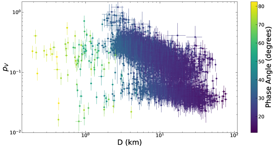
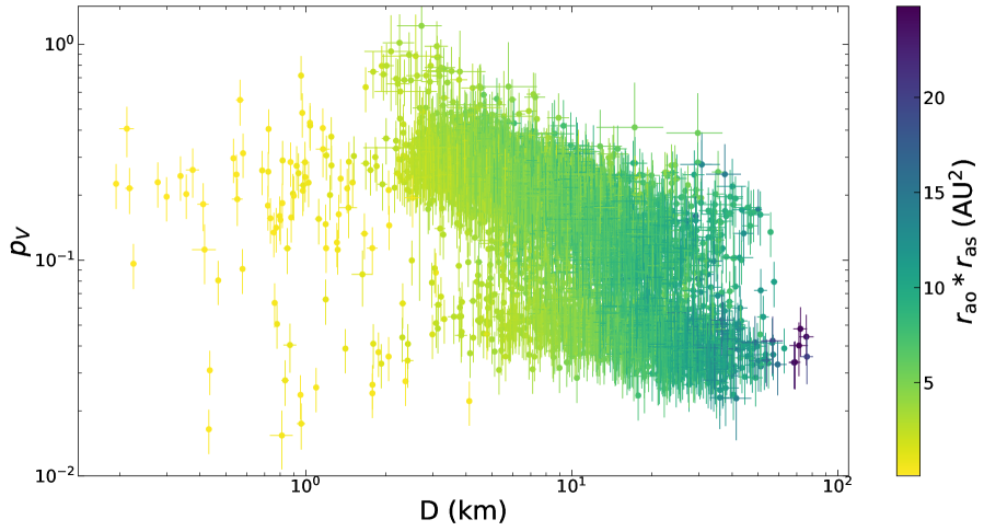
Figure 19 shows the visible-band geometric albedo $p_{\rm V}$ as a function of pseudo-temperature $T_{1}$ for 4685 asteroid fits.

Figure 19: Visible-band geometric albedo as a function of pseudo-temperature $T_{1}$ for the 4685 asteroid fits presented in this work.

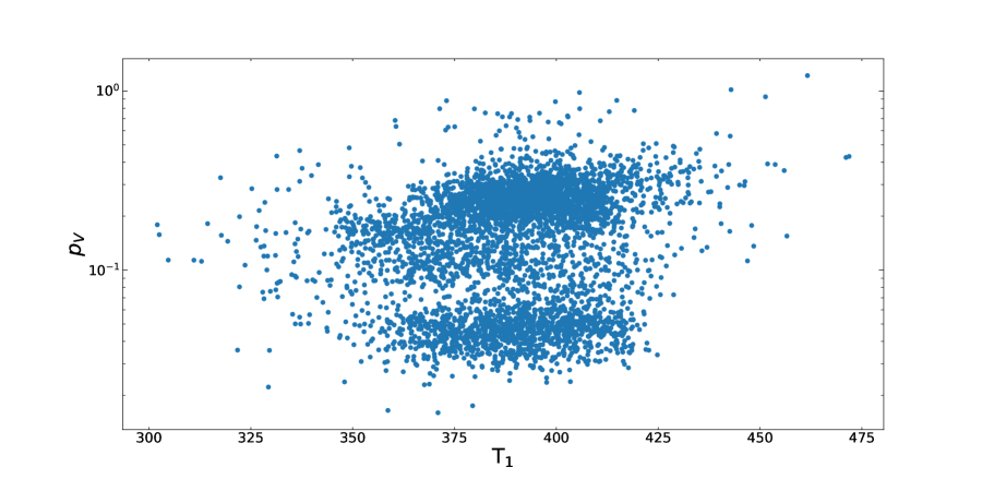
Figure 20 shows the distribution of the median phase angles $\alpha$ for 4685 asteroid fits.

Figure 20: Distribution of the median phase angles $\alpha$ for the 4685 asteroid fits presented in this work.

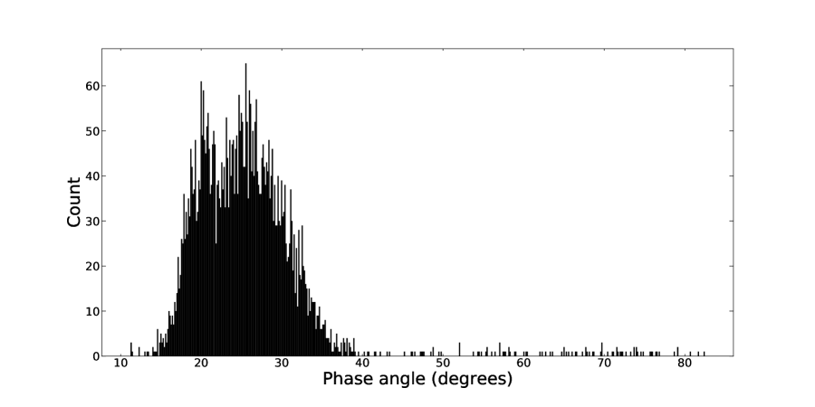
Figure 21 shows the median emissivity value $\epsilon_{\rm med}$ across all four WISE bands as a function of pseudo-temperature $T_{1}$ for 4685 asteroid fits.

Figure 21: Median emissivity value across all four WISE bands as a function of pseudo-temperature $T_{1}$ for the 4685 asteroid fits presented in this work.

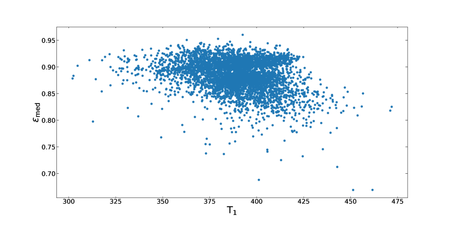
Figure 22 shows the beaming parameter $\eta$ as a function of the pseudo-temperature $T_{1}$ parameter for 4685 asteroid fits. The beaming parameter was not a free parameter in the thermal fits. Instead, it was calculated using Equation (8) with $\epsilon$ set to the median emissivity value across all four WISE bands.

Figure 22: Beaming parameter $\eta$ as a function of pseudo-temperature $T_{1}$ for the 4685 asteroid fits presented in this work.

References

- Abell et al. (2015) Abell, P. A., Barbee, B. W., Chodas, P. W., et al. 2015, in Asteroids IV, ed. P. Michel, F. E. DeMeo, & W. F. Bottke (Univ. of Arizona Press), 855–880, doi: 10.2458/azu_uapress_9780816532131-ch043
- Benner et al. (2015) Benner, L. A. M., Busch, M. W., Giorgini, J. D., Taylor, P. A., & Margot, J. L. 2015, in Asteroids IV, ed. P. Michel, F. E. DeMeo, & W. F. Bottke (Univ. of Arizona Press), 165–182, doi: 10.2458/azu_uapress_9780816530595-ch009
- Bottke et al. (2015) Bottke, W. F., Brož, M., O’Brien, D. P., et al. 2015, in Asteroids IV, ed. W. F. Bottke, A. Cellino, P. Paolicchi, & R. P. Binzel (Univ. of Arizona Press), 701–724, doi: 10.2458/azu_uapress_9780816532131-ch036
- Bottke et al. (2006) Bottke, Jr., W. F., Vokrouhlický, D., Rubincam, D. P., & Nesvorný, D. 2006, Annual Review of Earth and Planetary Sciences, 34, 157, doi: 10.1146/annurev.earth.34.031405.125154
- Bowell et al. (1989) Bowell, E., Hapke, B., Domingue, D., et al. 1989, in Asteroids II, ed. R. P. Binzel, T. Gehrels, & M. S. Matthews, 524–556
- Brown et al. (2014) Brown, M. J. I., Jarrett, T. H., & Cluver, M. E. 2014, Publications of the Astronomical Society of Australia, 31, e049, doi: 10.1017/pasa.2014.44
- Byrd et al. (1995) Byrd, R., Lu, P., Nocedal, J., & Zhu, C. 1995, SIAM Journal of Scientific Computing, 16, 1190, doi: 10.1137/0916069
- Coddington et al. (2016) Coddington, O., Lean, J. L., Pilewskie, P., Snow, M., & Lindholm, D. 2016, Bulletin of the American Meteorological Society, 97, 1265, doi: 10.1175/BAMS-D-14-00265.1
- Delbo et al. (2015) Delbo, M., Mueller, M., Emery, J. P., Rozitis, B., & Capria, M. T. 2015, Asteroid Thermophysical Modeling, ed. P. Michel, F. E. DeMeo, & W. F. Bottke, 107–128, doi: 10.2458/azu_uapress_9780816532131-ch006
- Dermott et al. (2021) Dermott, S. F., Li, D., Christou, A. A., et al. 2021, MNRAS, 505, 1917, doi: 10.1093/mnras/stab1390
- Farnocchia et al. (2015) Farnocchia, D., Chesley, S. R., Milani, A., Gronchi, G. F., & Chodas, P. W. 2015, in Asteroids IV, ed. P. Michel, F. E. DeMeo, & W. F. Bottke (Univ. of Arizona Press), 815–834, doi: 10.2458/azu_uapress_9780816532131-ch041
- Feigelson & Babu (2012) Feigelson, E. D., & Babu, G. J. 2012, Modern statistical methods for astronomy: with R applications (Cambridge University Press)
- Greenberg et al. (2020) Greenberg, A. H., Margot, J.-L., Verma, A. K., Taylor, P. A., & Hodge, S. E. 2020, The Astronomical Journal, 159, 92, doi: 10.3847/1538-3881/ab62a3
- Hanuš et al. (2015) Hanuš, J., Delbo’, M., Ďurech, J., & Alí-Lagoa, V. 2015, Icarus, 256, 101, doi: 10.1016/j.icarus.2015.04.014
- Hapke (2012) Hapke, B. 2012, Theory of reflectance and emittance spectroscopy (Cambridge university press)
- Harris (1998) Harris, A. W. 1998, Icarus, 131, 291, doi: https://doi.org/10.1006/icar.1997.5865
- Harris et al. (2015) Harris, A. W., Boslough, M., Chapman, C. R., et al. 2015, in Asteroids IV, ed. P. Michel, F. E. DeMeo, & W. F. Bottke (Univ. of Arizona Press), 835–854, doi: 10.2458/azu_uapress_9780816532131-ch042
- Harris & Lagerros (2002) Harris, A. W., & Lagerros, J. S. 2002, Asteroids III, 205
- Herald et al. (2019) Herald, D., Frappa, E., Gault, D., et al. 2019, Asteroid Occultations V3.0, urn:nasa:pds:smallbodiesoccultations::3.0. NASA Planetary Data System, doi: 10.26033/ap0g-wf63
- Herald et al. (2020) Herald, D., Gault, D., Anderson, R., et al. 2020, MNRAS, doi: 10.1093/mnras/staa3077
- Ivezić et al. (2014) Ivezić, Ž., Connolly, A. J., VanderPlas, J. T., & Gray, A. 2014, Statistics, data mining, and machine learning in astronomy (Princeton University Press)
- Mainzer et al. (2019) Mainzer, A., Bauer, J., Cutri, R., et al. 2019, NEOWISE Diameters and Albedos V2.0, urn:nasa:pds:neowise_diameters_albedos::2.0. NASA Planetary Data System, doi: 10.26033/18S3-2Z54
- Mainzer et al. (2015) Mainzer, A., Usui, F., & Trilling, D. E. 2015, in Asteroids IV, ed. P. Michel, F. E. DeMeo, & W. F. Bottke (Univ. of Arizona Press), 89–106, doi: 10.2458/azu_uapress_9780816532131-ch005
- Mainzer et al. (2011a) Mainzer, A., Bauer, J., Grav, T., et al. 2011a, ApJ, 731, 53, doi: 10.1088/0004-637X/731/1/53
- Mainzer et al. (2011b) Mainzer, A., Grav, T., Masiero, J., et al. 2011b, ApJ, 736, 100, doi: 10.1088/0004-637X/736/2/100
- Masiero et al. (2021) Masiero, J. R., Wright, E. L., & Mainzer, A. K. 2021, The Planetary Science Journal, 2, 32, doi: 10.3847/PSJ/abda4d
- Masiero et al. (2011) Masiero, J. R., Mainzer, A. K., Grav, T., et al. 2011, ApJ, 741, 68, doi: 10.1088/0004-637X/741/2/68
- Moeyens et al. (2020) Moeyens, J., Myhrvold, N., & Ivezić, Ž. 2020, Icarus, 341, 113575, doi: 10.1016/j.icarus.2019.113575
- Myhrvold (2018a) Myhrvold, N. 2018a, Icarus, 303, 91, doi: https://doi.org/10.1016/j.icarus.2017.12.024
- Myhrvold (2018b) —. 2018b, Icarus, 314, 64, doi: https://doi.org/10.1016/j.icarus.2018.05.004
- Neese (2010) Neese, C. 2010, NASA Planetary Data System, EAR
- Nesvorný et al. (2015) Nesvorný, D., Brož, M., & Carruba, V. 2015, in Asteroids IV, ed. P. Michel, F. E. DeMeo, & W. F. Bottke (Univ. of Arizona Press), 297–321, doi: 10.2458/azu_uapress_9780816532131-ch016
- Ostro et al. (2002) Ostro, S. J., Hudson, R. S., Benner, L. A. M., et al. 2002, in Asteroids III, ed. W. F. Bottke, A. Cellino, P. Paolicchi, & R. P. Binzel (Univ. of Arizona Press), 151–168
- Pravec et al. (2012) Pravec, P., Harris, A. W., Kušnirák, P., Galád, A., & Hornoch, K. 2012, Icarus, 221, 365 , doi: https://doi.org/10.1016/j.icarus.2012.07.026
- Ratkowsky (1983) Ratkowsky, D. 1983
- Scheeres et al. (2015) Scheeres, D. J., Britt, D., Carry, B., & Holsapple, K. A. 2015, in Asteroids IV, ed. P. Michel, F. E. DeMeo, & W. F. Bottke (Univ. of Arizona Press), 745–766, doi: 10.2458/azu_uapress_9780816532131-ch038
- Vereš et al. (2015) Vereš, P., Jedicke, R., Fitzsimmons, A., et al. 2015, Icarus, 261, 34 , doi: https://doi.org/10.1016/j.icarus.2015.08.007
- Warner, B.D. and Harris, A.W. and Pravec, P. (2021) Warner, B.D. and Harris, A.W. and Pravec, P. 2021, Asteroid Lightcurve Data Base (LCDB) Bundle V4.0., NASA Planetary Data System, doi: 10.26033/j3xc-3359
- Wright et al. (2018) Wright, E., Mainzer, A., Masiero, J., et al. 2018, arXiv e-prints, arXiv:1811.01454. https://arxiv.org/abs/1811.01454
- Wright (2019) Wright, E. L. 2019, in American Astronomical Society Meeting Abstracts, Vol. 233, American Astronomical Society Meeting Abstracts #233, 263.04
- Wright et al. (2010) Wright, E. L., Eisenhardt, P. R. M., Mainzer, A. K., et al. 2010, AJ, 140, 1868, doi: 10.1088/0004-6256/140/6/1868