Abstract

Many functions have approximately-known upper and/or lower bounds, potentially aiding the modeling of such functions. In this paper, we introduce Gaussian process models for functions where such bounds are (approximately) known. More specifically, we propose the first use of such bounds to improve Gaussian process (gp) posterior sampling and Bayesian optimization (bo). That is, we transform a gp model satisfying the given bounds, and then sample and weight functions from its posterior. To further exploit these bounds in bo settings, we present bounded entropy search (bes) to select the point gaining the most information about the underlying function, estimated by the gp samples, while satisfying the output constraints. We characterize the sample variance bounds and show that the decision made by bes is explainable. Our proposed approach is conceptually straightforward and can be used as a plugin extension to existing methods for gp posterior sampling and Bayesian optimization.


Gaussian Process Sampling and Optimization with Approximate Upper and Lower Bounds


Vu Nguyen                        Marc Peter Deisenroth                        Michael A. Osborne

Amazon                        University College London                        University of Oxford

1 Introduction

Gaussian processes (gp s) provide a powerful probabilistic learning framework that has led to great success in many machine learning settings, such as black-box optimization (Brochu et al.,, 2010), reinforcement learning (Deisenroth and Rasmussen,, 2011), hyperparameter tuning (Perrone et al.,, 2019; Parker-Holder et al.,, 2020), and battery forecasting (Richardson et al.,, 2017). gp s have been especially impactful for Bayesian optimization (bo) (Shahriari et al.,, 2016) to optimize a black-box function f()𝑓f(\cdot), where careful uncertainty representation is crucial. A fundamental challenge for Gaussian process modeling and optimization is that data are often limited. In bo, a datum is usually an expensive evaluation of another model. Particularly, we evaluate and optimize the underlying black-box without knowing the gradient or the analytical form of f()𝑓f(\cdot). In the small data regime, it is always useful to utilize external knowledge about f()𝑓f(\cdot) as has been successfully demonstrated in recent work, such as monotonicity trends (Riihimäki and Vehtari,, 2010), experimenter’s hunches (Li et al.,, 2018), and known optimum values (Nguyen and Osborne,, 2020).

We propose to use another form of prior knowledge for improving both the gp posterior sampling and Bayesian optimization. We consider the maximum and minimum values of f()𝑓f(\cdot). These optimal values can be found in machine learning applications, including inverse problems (Mosegaard and Tarantola,, 1995; Aster et al.,, 2018; Bertero and Boccacci,, 2020), where the goal is to retrieve an input 𝐱superscript𝐱\mathbf{x}^{*} resulting in the given target from a black-box function. Another example is tuning hyperparameters for classification algorithms (Krizhevsky et al.,, 2012); users may have vague knowledge about f+:=maxf()assignsuperscript𝑓𝑓f^{+}:=\max f(\cdot) and f:=minf()assignsuperscript𝑓𝑓f^{-}:=\min f(\cdot), either from recent state-of-the-art results or directly from the definition of the accuracy metric f+=100%superscript𝑓percent100f^{+}=100\%, f=0%superscript𝑓percent0f^{-}=0\%. Similar information can be found in tuning regression problems where the best root mean square error (rmse) score is known to be 00. Other examples are discussed by Nguyen and Osborne, (2020), such as known maximum rewards for some reinforcement learning environments. Despite the usefulness of such prior knowledge for the low-data regime, the setting we consider in this paper, with approximately known maximum and minimum values, is new to the best of our knowledge.

In this paper, we propose to exploit the knowledge of maximum and minimum values of the black-box for improving the performance of gp posterior sampling and making better decisions in bo, especially when the number of observations is limited. Rather than using a regular gp as a surrogate model to infer the underlying function f()𝑓f(\cdot), we transform the surrogate given the bound information. We assign different credits to samples based on the bounds and thus discard those falling outside. Moreover, we utilize these bounds for bo by proposing bounded entropy search (bes) to select the next point as that yielding the most information about the true underlying function. Our key contributions are:

  • the first use of exploiting knowledge about both the maximum f+superscript𝑓f^{+} and/or minimum fsuperscript𝑓f^{-} values of a black-box function, which can be approximately defined,

  • an efficient posterior sampling procedure for f()𝑓f(\cdot) that explicitly accounts for f+superscript𝑓f^{+} and fsuperscript𝑓f^{-},

  • a bounded entropy search (bes) acquisition function for bo given f+superscript𝑓f^{+} and fsuperscript𝑓f^{-}.

2 Preliminaries

A black-box f()𝑓f(\cdot) is defined over some bounded domain 𝒳d𝒳superscript𝑑\mathcal{X}\subset\mathbb{R}^{d} where d𝑑d is the input dimension. The function f𝑓f can only be accessed through noisy queries of the form yi𝒩(f(𝐱i),σf2)similar-tosubscript𝑦𝑖𝒩𝑓subscript𝐱𝑖superscriptsubscript𝜎𝑓2y_{i}\sim\mathcal{N}\bigl{(}f(\mathbf{x}_{i}),\sigma_{f}^{2}\bigr{)} where the input 𝐱idsubscript𝐱𝑖superscript𝑑\mathbf{x}_{i}\in\mathbb{R}^{d}, the output yisubscript𝑦𝑖y_{i}\in\mathbb{R}, and σf2superscriptsubscript𝜎𝑓2\sigma_{f}^{2} is the output noise variance. We denote 𝐗=[𝐱1,,𝐱N]TN×d𝐗superscriptsubscript𝐱1subscript𝐱𝑁𝑇superscript𝑁𝑑\mathbf{X}=[\mathbf{x}_{1},...,\mathbf{x}_{N}]^{T}\in\mathbb{R}^{N\times d}, 𝐲=[y1,,yN]TN×1𝐲superscriptsubscript𝑦1subscript𝑦𝑁𝑇superscript𝑁1\mathbf{y}=[y_{1},...,y_{N}]^{T}\in\mathbb{R}^{N\times 1}, and the training set at iteration t𝑡t by Dt={𝐱i,yi}i=1tsubscript𝐷𝑡superscriptsubscriptsubscript𝐱𝑖subscript𝑦𝑖𝑖1𝑡D_{t}=\{\mathbf{x}_{i},y_{i}\}_{i=1}^{t}.

2.1 Gaussian processes

We assume f𝑓f to be drawn from a gp (Rasmussen and Williams,, 2006) which is a random function f:𝒳:𝑓𝒳f:\mathcal{X}\rightarrow\mathbb{R}, such that every finite collection of those random variables f(𝐗)𝐗𝒳conditional𝑓subscript𝐗subscript𝐗𝒳f(\mathbf{X}_{*})\mid\mathbf{X}_{*}\in\mathcal{X} follows a multivariate Gaussian distribution. Formally, we denote a gp as f(𝐱)gp(m(𝐱),k(𝐱,𝐱))similar-to𝑓𝐱gp𝑚𝐱𝑘𝐱superscript𝐱f(\mathbf{x})\sim\lx@glossaries@gls@link{acronym}{GP}{\leavevmode\textsc{gp}}\bigl{(}m\left(\mathbf{x}\right),k\left(\mathbf{x},\mathbf{x}^{\prime}\right)\bigr{)}, where m(𝐱)=𝔼[f(𝐱)]𝑚𝐱𝔼delimited-[]𝑓𝐱m(\mathbf{x})=\mathbb{E}\left[f\left(\mathbf{x}\right)\right] and k(𝐱,𝐱)=𝔼[(f(𝐱)m(𝐱))T(f(𝐱)m(𝐱))]𝑘𝐱superscript𝐱𝔼delimited-[]superscript𝑓𝐱𝑚𝐱𝑇𝑓superscript𝐱𝑚superscript𝐱k(\mathbf{x},\mathbf{x}^{\prime})=\mathbb{E}\left[\bigl{(}f\left(\mathbf{x}\right)-m\left(\mathbf{x}\right)\bigr{)}^{T}\bigl{(}f\left(\mathbf{x}^{\prime}\right)-m\left(\mathbf{x}^{\prime}\right)\bigr{)}\right] are the mean and covariance functions. Given the observed input 𝐗𝐗\mathbf{X} and output 𝐲𝐲\mathbf{y}, the gp posterior at a new input 𝐱subscript𝐱\mathbf{x}_{*} is defined as f𝐗,𝐲,𝐱𝒩(μ(𝐱),σ2(𝐱))similar-toconditionalsubscript𝑓𝐗𝐲subscript𝐱𝒩𝜇subscript𝐱superscript𝜎2subscript𝐱f_{*}\mid\mathbf{X},\mathbf{y},\mathbf{x}_{*}\sim\mathcal{N}\left(\mu\left(\mathbf{x}_{*}\right),\sigma^{2}\left(\mathbf{x}_{*}\right)\right). The posterior predictive mean and variance are:

μ(𝐱)=𝜇subscript𝐱absent\displaystyle\mu\left(\mathbf{x}_{*}\right)=\; 𝐤T[𝐊+σf2𝐈]1(𝐲𝐦)+m(𝐱)subscriptsuperscript𝐤𝑇superscriptdelimited-[]𝐊subscriptsuperscript𝜎2𝑓𝐈1𝐲𝐦𝑚subscript𝐱\displaystyle\mathbf{k}^{T}_{*}\left[\mathbf{K}+\sigma^{2}_{f}\mathbf{I}\right]^{-1}\left(\mathbf{y}-\mathbf{m}\right)+m(\mathbf{x}_{*}) (1)
σ2(𝐱)=superscript𝜎2subscript𝐱absent\displaystyle\sigma^{2}\left(\mathbf{x}_{*}\right)=\; k𝐤T[𝐊+σf2𝐈]1𝐤subscript𝑘absentsubscriptsuperscript𝐤𝑇superscriptdelimited-[]𝐊subscriptsuperscript𝜎2𝑓𝐈1subscript𝐤\displaystyle k_{**}-\mathbf{k}^{T}_{*}\left[\mathbf{K}+\sigma^{2}_{f}\mathbf{I}\right]^{-1}\mathbf{k}_{*} (2)

where k=k(𝐱,𝐱)subscript𝑘absent𝑘subscript𝐱subscript𝐱k_{**}=k\left(\mathbf{x}_{*},\mathbf{x}_{*}\right), 𝐤=[k(𝐱,𝐱i)]iTN×1subscript𝐤subscriptsuperscriptdelimited-[]𝑘subscript𝐱subscript𝐱𝑖𝑇for-all𝑖superscript𝑁1\mathbf{k}_{*}=[k\left(\mathbf{x}_{*},\mathbf{x}_{i}\right)]^{T}_{\forall i}\in\mathbb{R}^{N\times 1}, 𝐦=[m(𝐱i)]iTN×1𝐦subscriptsuperscriptdelimited-[]𝑚subscript𝐱𝑖𝑇for-all𝑖superscript𝑁1\mathbf{m}=[m\left(\mathbf{x}_{i}\right)]^{T}_{\forall i}\in\mathbb{R}^{N\times 1} is the prior mean at the observed locations and 𝐊=[k(𝐱i,𝐱j)]i,jN×N𝐊subscriptdelimited-[]𝑘subscript𝐱𝑖subscript𝐱𝑗for-all𝑖𝑗superscript𝑁𝑁\mathbf{K}=\left[k\left(\mathbf{x}_{i},\mathbf{x}_{j}\right)\right]_{\forall i,j}\in\mathbb{R}^{N\times N}.

Samples g()gp(μ(),σ2())similar-to𝑔gp𝜇superscript𝜎2g(\cdot)\sim\lx@glossaries@gls@link{acronym}{GP}{\leavevmode\textsc{gp}}\bigl{(}\mu(\cdot),\sigma^{2}(\cdot)\bigr{)} from a gp posterior can be used for several applications, e.g., Thompson sampling (ts) (Thompson,, 1933; Russo et al.,, 2018), or an information-theoretic decision in bo (Hernández-Lobato et al.,, 2014, 2017; Kirthevasan et al.,, 2018). We follow the decoupled approach (Wilson et al.,, 2020, 2021) to draw samples g()𝑔g(\cdot) from a gp posterior. The central idea of decoupled sampling relies on Matheron’s rule for Gaussian random variables (Journel and Huijbregts,, 1978; Chiles and Delfiner,, 2009; Doucet,, 2010), using variational Fourier features for an approximate prior and a deterministic data-dependent update term. The key benefit of this sampling is that the complexity scales linearly in the number of test points. This is particularly useful in optimizing the acquisition function in bo where we need to evaluate at many test points to select a next query.

2.2 Optimum values prior in Bayesian optimization

bo aims at maximizing an expensive black-box function f()𝑓f(\cdot) using few function evaluations, i.e. finding 𝐱:=argmax𝐱𝒳f(𝐱)assignsuperscript𝐱subscript𝐱𝒳𝑓𝐱\mathbf{x}^{*}:=\arg\max_{\mathbf{x}\in\mathcal{X}}f(\mathbf{x}). In bo, we typically construct a surrogate model of f𝑓f using a gp. The surrogate model mimics the behavior of f𝑓f while it is cheaper to evaluate. Then, we sequentially select points 𝐱tsubscript𝐱𝑡\mathbf{x}_{t} at which to evaluate f𝑓f.

Prior knowledge about the optimum value of the black-box contains useful information dictating the upper bound of f()𝑓f(\cdot). A recent approach has considered the bo setting where the true optimum value f+=max𝐱𝒳f(𝐱)superscript𝑓subscript𝐱𝒳𝑓𝐱f^{+}=\max_{\mathbf{x}\in\mathcal{X}}f(\mathbf{x}) of the black-box function is available (Nguyen and Osborne,, 2020). In particular, they transform the gp surrogate to satisfy that f+superscript𝑓f^{+} is an upper bound, and propose expected regret minimization (erm) and confidence bound minimization (cbm) acquisition functions. However, this approach can be ineffective when the value of the true optimum maxf()𝑓\max f(\cdot) is not known. If the optimum value is mis-specified, the performance degrades. In addition, this approach can only cope with knowledge of f+superscript𝑓f^{+}, but it is unable to account for knowledge of both f+superscript𝑓f^{+} and fsuperscript𝑓f^{-} at the same time. The method we propose in this paper will overcome these limitations.

3 Gaussian process posterior sampling with approximate bounds f+superscript𝑓f^{+} and fsuperscript𝑓f^{-}

We consider settings where we know approximately the maximum and/or minimum value of f𝑓f. We express the prior knowledge about the upper bound by specifying the value of f+superscript𝑓f^{+} and how loosely such bound via η+subscript𝜂\eta_{+}. Similar design is for the lower bound via fsuperscript𝑓f^{-} and ηsubscript𝜂\eta_{-}.

Definition 1.

Define the approximate bounds as random variables: f+𝒩(maxf,η+2)similar-tosuperscript𝑓𝒩𝑓subscriptsuperscript𝜂2f^{+}\sim\mathcal{N}(\max f,\eta^{2}_{+}) and f𝒩(minf,η2)similar-tosuperscript𝑓𝒩𝑓subscriptsuperscript𝜂2f^{-}\sim\mathcal{N}(\min f,\eta^{2}_{-}).

We may observe both f+superscript𝑓f^{+} and fsuperscript𝑓f^{-} or either of them. The useful information f+superscript𝑓f^{+} and fsuperscript𝑓f^{-} give us is that (i) f()𝑓f(\cdot) should not exceed these thresholds and (ii) f()𝑓f(\cdot) should attain closely f+,fsuperscript𝑓superscript𝑓f^{+},f^{-}. In particular, for maximization problems, the location at which f+superscript𝑓f^{+} is attained, is potentially the global maximizer of f𝑓f we are looking for in bo settings.

Refer to caption
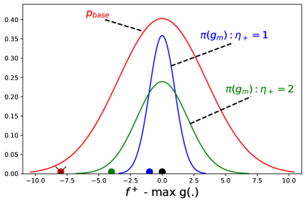
Figure 1: Illustration of the sampling and weighting step. Left: We can use a gp or a srgp for pbasesubscript𝑝basep_{\textrm{base}}. Given the same weighting probability π(gm)𝜋subscript𝑔𝑚\pi(g_{m}), using srgp has a smaller sample variance by ignoring the redundant space (orange area). Right: For ease of representation, we use a univariate Gaussian distribution to visualize π(gm)𝜋subscript𝑔𝑚\pi(g_{m}). The gp sample gm()subscript𝑔𝑚g_{m}(\cdot) (represented by the maximum value of gm()subscript𝑔𝑚g_{m}(\cdot)) is drawn from pbasesubscript𝑝basep_{\textrm{base}}. We assign high weight to a sample depending on the density of π(gm)𝜋subscript𝑔𝑚\pi(g_{m}). The red point will be rejected. The green point falls within the density of π(gm)𝜋subscript𝑔𝑚\pi(g_{m}) with η+=2subscript𝜂2\eta_{+}=2, but not for η+=1subscript𝜂1\eta_{+}=1. The blue point receives positive weights by both π(gm)𝜋subscript𝑔𝑚\pi(g_{m}) including η+=1subscript𝜂1\eta_{+}=1 and η+=2subscript𝜂2\eta_{+}=2. The black point receives the highest weight.

3.1 Sampling and weighting gp posterior samples

Although the existing gp posterior sampling approach (Wilson et al.,, 2020) has demonstrated great success, the resulting gp samples usually do not obey the bounds [f,f+]superscript𝑓superscript𝑓[f^{-},f^{+}]. Intuitively, assume we are given a few (noisy) observations from the black-box f𝑓f. We can be confident in deciding which gp samples are not admissible by looking at the bounds f+,fsuperscript𝑓superscript𝑓f^{+},f^{-} and thus not making use of these samples. Therefore, we propose to assign different credits to the gp samples based on the bound knowledge.

We denote pbasesubscript𝑝basep_{\textrm{base}} the base distribution to generate gp posterior samples, e.g., using decoupling approach (Wilson et al.,, 2020). Given the constraints f+,fsuperscript𝑓superscript𝑓f^{+},f^{-}, we can perform weighted-averaging across all gp samples as:

g^^𝑔\displaystyle\hat{g} :=gmpbasegmp(f+,fgm)p(f+,fgm)=m=1Mgmπ(gm)m=1Mπ(gm)assignabsentsubscriptsimilar-tosubscript𝑔𝑚subscript𝑝𝑏𝑎𝑠𝑒subscript𝑔𝑚𝑝superscript𝑓conditionalsuperscript𝑓subscript𝑔𝑚𝑝superscript𝑓conditionalsuperscript𝑓subscript𝑔𝑚superscriptsubscript𝑚1𝑀subscript𝑔𝑚𝜋subscript𝑔𝑚superscriptsubscript𝑚1𝑀𝜋subscript𝑔𝑚\displaystyle:=\sum_{g_{m}\sim p_{base}}g_{m}\frac{p(f^{+},f^{-}\mid g_{m})}{\sum p(f^{+},f^{-}\mid g_{m})}=\sum_{m=1}^{M}g_{m}\frac{\pi(g_{m})}{\sum_{m=1}^{M}\pi(g_{m})} (3)

where gmsubscript𝑔𝑚g_{m} is a gp posterior sample, see Eq. (17) in the appendix for details. We denote π(gm):=p(f+,fgm)assign𝜋subscript𝑔𝑚𝑝superscript𝑓conditionalsuperscript𝑓subscript𝑔𝑚\pi(g_{m}):=p\Bigl{(}f^{+},f^{-}\mid g_{m}\Bigr{)} which assigns high probability to a sample gmsubscript𝑔𝑚g_{m} satisfying the approximate bounds while it assigns zero or very low probability otherwise. The fraction of π(gm)m=1Mπ(gm)𝜋subscript𝑔𝑚superscriptsubscript𝑚1𝑀𝜋subscript𝑔𝑚\frac{\pi(g_{m})}{\sum_{m=1}^{M}\pi(g_{m})} indicates the normalized weight of a sample m𝑚m. We define π(gm)𝜋subscript𝑔𝑚\pi(g_{m}) in the next section.

3.2 The weighting probability π(gm)𝜋subscript𝑔𝑚\pi(g_{m}) given f+superscript𝑓f^{+} and fsuperscript𝑓f^{-}

Given the data 𝐗,𝐲𝐗𝐲\mathbf{X},\mathbf{y}, we draw M𝑀M samples from a gp posterior and expect that a gp sample gm()subscript𝑔𝑚g_{m}(\cdot) naturally follows the conditions: (i) fgm()f+less-than-or-similar-tosuperscript𝑓subscript𝑔𝑚less-than-or-similar-tosuperscript𝑓f^{-}\lesssim g_{m}(\cdot)\lesssim f^{+} and (ii) 𝐱m+superscriptsubscript𝐱𝑚\exists\mathbf{x}_{m}^{+} such that gm(𝐱m+)f+subscript𝑔𝑚superscriptsubscript𝐱𝑚superscript𝑓g_{m}(\mathbf{x}_{m}^{+})\approx f^{+} and 𝐱msuperscriptsubscript𝐱𝑚\exists\mathbf{x}_{m}^{-} such that gm(𝐱m)fsubscript𝑔𝑚superscriptsubscript𝐱𝑚superscript𝑓g_{m}(\mathbf{x}_{m}^{-})\approx f^{-}. Let us denote the maximum and minimum values of the sample by gm+=maxgm()subscriptsuperscript𝑔𝑚subscript𝑔𝑚g^{+}_{m}=\max g_{m}(\cdot) and gm=mingm()subscriptsuperscript𝑔𝑚subscript𝑔𝑚g^{-}_{m}=\min g_{m}(\cdot) which can be computed efficiently using the off-the-shelf toolboxes, such as multi-start gradient descent György and Kocsis, (2011) because we have the analytical form available for gm()subscript𝑔𝑚g_{m}(\cdot), presented in Appendix B.3. To satisfy the above conditions, we define the weighting probability π(gm)𝜋subscript𝑔𝑚\pi(g_{m}) using an isotropic bivariate Gaussian distribution:

π(gm)𝜋subscript𝑔𝑚\displaystyle\pi(g_{m}) :=𝒩([gm,gm+][f,f+],diag[η2,η+2]).assignabsent𝒩conditionalsubscriptsuperscript𝑔𝑚subscriptsuperscript𝑔𝑚superscript𝑓superscript𝑓diagsubscriptsuperscript𝜂2subscriptsuperscript𝜂2\displaystyle:=\mathcal{N}\Big{(}\left[g^{-}_{m},g^{+}_{m}\right]\mid\left[f^{-},f^{+}\right],\text{diag}[\eta^{2}_{-},\eta^{2}_{+}]\Big{)}. (4)

The mean of π(gm)𝜋subscript𝑔𝑚\pi(g_{m}) is located at [f,f+]superscript𝑓superscript𝑓[f^{-},f^{+}] and the M𝑀M observations [gm,gm+]subscriptsuperscript𝑔𝑚subscriptsuperscript𝑔𝑚\left[g^{-}_{m},g^{+}_{m}\right] are the min and max values of the gp posterior samples, see Fig. 1 (left). This bivariate will flexibly collapse into a univariate Gaussian when either f+superscript𝑓f^{+} or fsuperscript𝑓f^{-} is observed.

Table 1: Acceptance ratio over M=200𝑀200M=200 samples from gp and srgp respectively. srgp can generate better samples by incorporating f+superscript𝑓f^{+} and Var[pbase-srgp]Var[pbase-gp]Vardelimited-[]subscript𝑝base-srgpVardelimited-[]subscript𝑝base-gp\textrm{Var}[p_{\textrm{base-\lx@glossaries@gls@link{acronym}{SRGP}{\leavevmode{srgp}}}}]\leq\textrm{Var}[p_{\textrm{base-\lx@glossaries@gls@link{acronym}{GP}{\leavevmode{gp}}}}]. See Section 5 for detail.
η+=η=0.5dsubscript𝜂subscript𝜂0.5𝑑\eta_{+}=\eta_{-}=0.5d η+=η=1dsubscript𝜂subscript𝜂1𝑑\eta_{+}=\eta_{-}=1d
gp srgp gp srgp
branin d=2 .39(.2).39.2.39(.2) .89(.2).89.2\mathbf{.89(.2)} .62(.1).62.1.62(.1) .96(.2).96.2\mathbf{.96(.2)}
rosenbrock d=2 .52(.2).52.2.52(.2) .88(.2).88.2\mathbf{.88(.2)} .62(.2).62.2.62(.2) .95(.2).95.2\mathbf{.95(.2)}
mccormick d=2 .65(.1).65.1.65(.1) .91(.2).91.2\mathbf{.91(.2)} .69(.1).69.1.69(.1) 1.0(.1)1.0.1\mathbf{1.0(.1)}
hartmann d=3 .08(.1).08.1.08(.1) .40(.3).40.3\mathbf{.40(.3)} .31(.2).31.2.31(.2) .76(.2).76.2\mathbf{.76(.2)}
alpine1 d=5 .0(.0).0.0.0(.0) .13(.1).13.1\mathbf{.13(.1)} .10(.1).10.1.10(.1) .30(.2).30.2\mathbf{.30(.2)}
gSobol d=5 .01(.1).01.1.01(.1) .46(.3).46.3\mathbf{.46(.3)} .14(.2).14.2.14(.2) .74(.4).74.4\mathbf{.74(.4)}

The view of rejection sampling.

The weighting scheme above can be seen from the rejection-sampling perspective. We accept a gp sample gm()subscript𝑔𝑚g_{m}(\cdot) if it lies within a two standard deviation band around the mean of π(gm)𝜋subscript𝑔𝑚\pi(g_{m}) as illustrated in Fig. 1 (right). Specifying a smaller value for η+subscript𝜂\eta_{+} will make π(gm)𝜋subscript𝑔𝑚\pi(g_{m}) strict and only accept a gp sample which has the maximum value maxgm()subscript𝑔𝑚\max g_{m}(\cdot) closer to f+superscript𝑓f^{+}. On the other hand, increasing η+,ηsubscript𝜂subscript𝜂\eta_{+},\eta_{-} will lead to more accepted samples, but in lower quality. We visualize π(gm)𝜋subscript𝑔𝑚\pi(g_{m}) using different values of η={1,2}𝜂12\eta=\{1,2\} in Fig. 1 (right) where we have simplified the 2d space into one dimension for better representation.

3.3 Square-root gp for sampling gmsubscript𝑔𝑚g_{m}

Algorithm 1 srgp-weighting with f+,fsuperscript𝑓superscript𝑓f^{+},f^{-}
1:  Input: #GP sample M𝑀M, data D𝐷D, f+superscript𝑓f^{+}, fsuperscript𝑓f^{-}
2:  Learn a srgp posterior model 𝒢𝒢\mathcal{G} from D𝐷{D} and f+superscript𝑓f^{+}
3:  Draw gp samples g1,.gMformulae-sequencesubscript𝑔1subscript𝑔𝑀g_{1},....g_{M} from pbasesubscript𝑝basep_{\textrm{base}} by (i) drawing from μh()subscript𝜇\mu_{h}(\cdot) and (ii) computing μf()subscript𝜇𝑓\mu_{f}(\cdot) in Eq. (6)
4:  Compute π(gm),m=1,,Mformulae-sequence𝜋subscript𝑔𝑚for-all𝑚1𝑀\pi(g_{m}),\forall m=1,...,M by Eq. (4)
5:  Output: g^(𝐱)=m=1Mgm(𝐱)π(gm)^𝑔𝐱superscriptsubscript𝑚1𝑀subscript𝑔𝑚𝐱𝜋subscript𝑔𝑚\hat{g}(\mathbf{x})=\sum_{m=1}^{M}g_{m}(\mathbf{x})\pi(g_{m})

We utilize Matheron’s rule to efficiently draw samples from a gp through pbasesubscript𝑝basep_{\textrm{base}}. However, taking a standard gp model for pbasesubscript𝑝basep_{\textrm{base}} can lead to unwanted samples being taken, as demonstrated empirically in Table 1 especially for high-dimensional functions such as alpine1 and gSobol. Here, we consider a sample is accepted when the density of π(gm)𝜋subscript𝑔𝑚\pi(g_{m}) is within two standard deviation of the Gaussian distribution defined in Eq. (4) and rejected otherwise.

Therefore, we propose to use a transformed gp surrogate model given f+superscript𝑓f^{+} for pbasesubscript𝑝basep_{\textrm{base}}, using a technique presented by Gunter et al., (2014). Based on Definition 1, we have that f+[maxf(𝐱)2η+,maxf(𝐱)+2η+]superscript𝑓𝑓𝐱2subscript𝜂𝑓𝐱2subscript𝜂f^{+}\in\big{[}\max f(\mathbf{x})-2\eta_{+},\max f(\mathbf{x})+2\eta_{+}\big{]}1112η+2subscript𝜂2\eta_{+} is chosen to cover 95%percent9595\% of the probability density with high probability. Therefore, we can write 𝐱,f(𝐱)f++2η+for-all𝐱𝑓𝐱superscript𝑓2subscript𝜂\forall\mathbf{x},f(\mathbf{x})\leq f^{+}+2\eta_{+}. Thus, there exists h()h(\cdot) satisfying 𝐱,f(𝐱)=f++2η+½h2(𝐱)for-all𝐱𝑓𝐱superscript𝑓2subscript𝜂½superscript2𝐱\forall\mathbf{x},f(\mathbf{x})=f^{+}+2\eta_{+}-½h^{2}(\mathbf{x}). Formally, we define f()𝑓f(\cdot) via h()gpsimilar-togph(\cdot)\sim\lx@glossaries@gls@link{acronym}{GP}{\leavevmode\textsc{gp}} as follows:

f()𝑓\displaystyle f(\cdot) =f++2η+12h2(),where hgp(mh,Kh).formulae-sequenceabsentsuperscript𝑓2subscript𝜂12superscript2similar-towhere gpsubscript𝑚subscript𝐾\displaystyle=f^{+}+2\eta_{+}-\tfrac{1}{2}h^{2}(\cdot),\quad\text{where }h\sim\lx@glossaries@gls@link{acronym}{GP}{\leavevmode\textsc{gp}}(m_{h},K_{h}). (5)

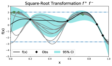
This transformation ensures the resulting function f()𝑓f(\cdot) to satisfy the bounded constraints f+f()greater-than-or-equivalent-tosuperscript𝑓𝑓f^{+}\gtrsim f(\cdot) and 𝐱+,f(𝐱+)f+superscript𝐱𝑓superscript𝐱superscript𝑓\exists\mathbf{x}^{+},f(\mathbf{x}^{+})\rightarrow f^{+} when h(𝐱+)0superscript𝐱0h(\mathbf{x}^{+})\rightarrow 0. We refer to Fig. 2 (bottom right) for an illustration of this transformation.

We estimate a posterior for drawing samples of h()h(\cdot) as follows. Denote the data in the original space by Df={𝐱i,yi}i=1Nsubscript𝐷𝑓superscriptsubscriptsubscript𝐱𝑖subscript𝑦𝑖𝑖1𝑁D_{f}=\{\mathbf{x}_{i},y_{i}\}_{i=1}^{N}, we compute Dh={𝐱i,hi}i=1Nsubscript𝐷superscriptsubscriptsubscript𝐱𝑖subscript𝑖𝑖1𝑁D_{h}=\{\mathbf{x}_{i},h_{i}\}_{i=1}^{N} where hi=2(f++2η+yi)subscript𝑖2superscript𝑓2subscript𝜂subscript𝑦𝑖h_{i}=\sqrt{2(f^{+}+2\eta_{+}-y_{i})}. Next we write the posterior of p(h(𝐱)Dh)𝒩(μh(𝐱),σh2(𝐱))𝑝conditionalsubscript𝐱subscript𝐷𝒩subscript𝜇subscript𝐱subscriptsuperscript𝜎2subscript𝐱p\left(h(\mathbf{x}_{*})\mid D_{h}\right)\approx\mathcal{N}\left(\mu_{h}(\mathbf{x}_{*}),\sigma^{2}_{h}(\mathbf{x}_{*})\right) with μh(𝐱)=mh(𝐱)+𝐤T[𝐊+σh2𝐈]1(𝒉mh)subscript𝜇subscript𝐱subscript𝑚subscript𝐱subscriptsuperscript𝐤𝑇superscriptdelimited-[]𝐊superscriptsubscript𝜎2𝐈1𝒉subscript𝑚\mu_{h}(\mathbf{x}_{*})=m_{h}(\mathbf{x}_{*})+\mathbf{k}^{T}_{*}\left[\mathbf{K}+\sigma_{h}^{2}\mathbf{I}\right]^{-1}\left(\boldsymbol{h}-m_{h}\right) and σ2(𝐱)=k𝐤T[𝐊+σh2𝐈]1𝐤superscript𝜎2subscript𝐱subscript𝑘absentsubscriptsuperscript𝐤𝑇superscriptdelimited-[]𝐊superscriptsubscript𝜎2𝐈1subscript𝐤\sigma^{2}\left(\mathbf{x}_{*}\right)=k_{**}-\mathbf{k}^{T}_{*}\left[\mathbf{K}+\sigma_{h}^{2}\mathbf{I}\right]^{-1}\mathbf{k}_{*} where σh2superscriptsubscript𝜎2\sigma_{h}^{2} is the measurement noise variance of h()h(\cdot) and other variables are defined analogously to Section 2.1.
Refer to caption
Refer to caption
Refer to caption
Refer to caption
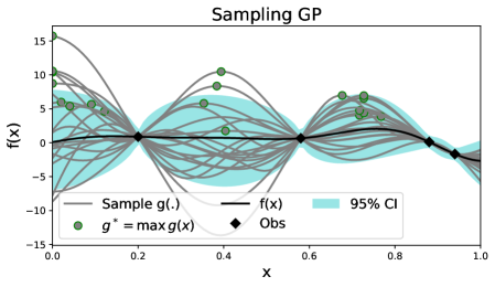
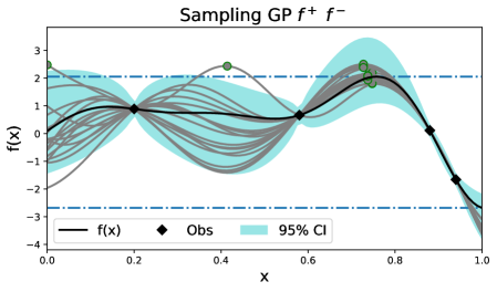
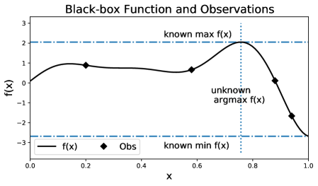
Figure 2: Top Right: Decoupled gp sampling (Wilson et al.,, 2020) given four observations from f(𝐱)𝑓𝐱f(\mathbf{x}). Bottom Left: gp sampling and weighting with both f+superscript𝑓f^{+} and fsuperscript𝑓f^{-}. Bottom Right: gp sampling and weighting with square-root transformation (or srgp. Given limited observations, the existing gp sampling can be misleading to fluctuate widely beyond the bounds (see the y-axis) while exploiting f+superscript𝑓f^{+} and fsuperscript𝑓f^{-} can result in better gp sample.

We draw gp samples from h()h(\cdot) to get f()𝑓f(\cdot) using Eq. (5). The resulting samples of f()𝑓f(\cdot) follow the upper bound conditions as desired—staying below f+superscript𝑓f^{+} and reaching (closely) the optimum value. After using f+superscript𝑓f^{+} to sample f()𝑓f(\cdot), we further exploit fsuperscript𝑓f^{-} via the weighting scheme using Eq. (4).

To estimate the posterior predictive mean and variance in the original space, we use a Taylor expansion to approximate the posterior predictive distribution (Gunter et al.,, 2014) p(f(𝐱)𝐗,𝐲,η+,f+)𝒩(μf,σf2)𝑝conditional𝑓subscript𝐱𝐗𝐲subscript𝜂superscript𝑓𝒩subscript𝜇𝑓subscriptsuperscript𝜎2𝑓p\big{(}f(\mathbf{x}_{*})\mid\mathbf{X},\mathbf{y},\eta_{+},f^{+}\big{)}\approx\mathcal{N}(\mu_{f},\sigma^{2}_{f}) where

μf(𝐱)=f++2η+12μh2(𝐱)subscript𝜇𝑓subscript𝐱superscript𝑓2subscript𝜂12superscriptsubscript𝜇2subscript𝐱\displaystyle\mu_{f}(\mathbf{x}_{*})=f^{+}+2\eta_{+}-\tfrac{1}{2}\mu_{h}^{2}(\mathbf{x}_{*}) (6)
σf2(𝐱)=μh(𝐱)σh2(𝐱)μh(𝐱).subscriptsuperscript𝜎2𝑓subscript𝐱subscript𝜇subscript𝐱subscriptsuperscript𝜎2subscript𝐱subscript𝜇subscript𝐱\displaystyle\sigma^{2}_{f}(\mathbf{x}_{*})=\mu_{h}(\mathbf{x}_{*})\sigma^{2}_{h}(\mathbf{x}_{*})\mu_{h}(\mathbf{x}_{*}). (7)

Taylor expansion gives the best possible approximation at the mode which is a multivariate function. This mode is set to μgsubscript𝜇𝑔\mu_{g} which is well approximated and thus for the resulting μfsubscript𝜇𝑓\mu_{f} and σfsubscript𝜎𝑓\sigma_{f}. We derive the above equations in Appendix B.5 and summarize the above process in Algorithm 1.

3.4 Tightening the variances of gp posterior samples

The base distribution pbasesubscript𝑝basep_{\textrm{base}} for drawing gp posterior samples in Eq. (3) can be used as (i) a standard gp (Wilson et al.,, 2020), (ii) weighting using gp or (iii) weighting using srgp (presented in Section 3.3), respectively. For brevity, we denote these approaches as pgpsubscript𝑝gpp_{\lx@glossaries@gls@link{acronym}{GP}{\leavevmode\textsc{gp}}}, pw-gpsubscript𝑝w-gpp_{\textrm{w-}\lx@glossaries@gls@link{acronym}{GP}{\leavevmode\textsc{gp}}} and pw-srgpsubscript𝑝w-srgpp_{\textrm{w-}\lx@glossaries@gls@link{acronym}{SRGP}{\leavevmode\textsc{srgp}}}.

We show that our approaches pw-gpsubscript𝑝w-gpp_{\textrm{w-}\lx@glossaries@gls@link{acronym}{GP}{\leavevmode\textsc{gp}}} and pw-srgpsubscript𝑝w-srgpp_{\textrm{w-}\lx@glossaries@gls@link{acronym}{SRGP}{\leavevmode\textsc{srgp}}} tighten the sample variance relative to pgpsubscript𝑝gpp_{\lx@glossaries@gls@link{acronym}{GP}{\leavevmode\textsc{gp}}} ignoring the bounds f+superscript𝑓f^{+}, fsuperscript𝑓f^{-}. We state the main theoretical results and refer to Appendix B.4 for the proofs.

Lemma 1.

In the 2d space formed by [f+,f]superscript𝑓superscript𝑓\left[f^{+},f^{-}\right] and the gp posterior samples {gm+,gm}m=1Msuperscriptsubscriptsubscriptsuperscript𝑔𝑚subscriptsuperscript𝑔𝑚𝑚1𝑀\{g^{+}_{m},g^{-}_{m}\}_{m=1}^{M}, the sample variances by weighting srgp and gp are smaller than the gp posterior sampling (Wilson et al.,, 2020) making no use of the bounds: Var[pw-gp]Var[pgp]Vardelimited-[]subscript𝑝w-gpVardelimited-[]subscript𝑝gp{\displaystyle\text{Var}\left[p_{\textrm{w-}\lx@glossaries@gls@link{acronym}{GP}{\leavevmode\textsc{gp}}}\right]}\leq{\displaystyle\text{Var}\left[p_{\lx@glossaries@gls@link{acronym}{GP}{\leavevmode\textsc{gp}}}\right]} and Var[pw-srgp]Var[pgp]Vardelimited-[]subscript𝑝w-srgpVardelimited-[]subscript𝑝gp{\displaystyle\text{Var}\left[p_{\textrm{w-}\lx@glossaries@gls@link{acronym}{SRGP}{\leavevmode\textsc{srgp}}}\right]}\leq{\displaystyle\text{Var}\left[p_{\lx@glossaries@gls@link{acronym}{GP}{\leavevmode\textsc{gp}}}\right]}.

To intuitively understand our analysis, we visualize these variances in the 2d space in Fig. 1 (left), created by [f+,f]superscript𝑓superscript𝑓\left[f^{+},f^{-}\right] and {gm+,gm}m=1Msuperscriptsubscriptsubscriptsuperscript𝑔𝑚subscriptsuperscript𝑔𝑚𝑚1𝑀\{g^{+}_{m},g^{-}_{m}\}_{m=1}^{M} taken from gp posterior samples. In Lemma 1, the sample variances using our approaches will be smaller than the approach in Wilson et al., (2020), which makes no use of the bounds. This highlights the benefit of using the bounds to eliminate bad samples, which violate the bounds, to obtain a smaller sample variance.

Next, we show in Lemma 2 that using pw-srgpsubscript𝑝w-srgpp_{\textrm{w-}\lx@glossaries@gls@link{acronym}{SRGP}{\leavevmode\textsc{srgp}}} will be more sample-efficient than using pw-gpsubscript𝑝w-gpp_{\textrm{w-}\lx@glossaries@gls@link{acronym}{GP}{\leavevmode\textsc{gp}}}. In other words, we get more accepted samples by using the weighting srgp, given the same number of posterior samples M𝑀M.

Lemma 2.

In the 2d space formed by [f+,f]superscript𝑓superscript𝑓\left[f^{+},f^{-}\right] and the gp posterior samples {gm+,gm}m=1Msuperscriptsubscriptsubscriptsuperscript𝑔𝑚subscriptsuperscript𝑔𝑚𝑚1𝑀\{g^{+}_{m},g^{-}_{m}\}_{m=1}^{M}, the sample variance of weighting srgp is smaller than weighting gp: Var[pw-srgp]Var[pw-gp]Vardelimited-[]subscript𝑝w-srgpVardelimited-[]subscript𝑝w-gp\text{Var}\left[p_{\textrm{w-\lx@glossaries@gls@link{acronym}{SRGP}{\leavevmode{srgp}}}}\right]\leq{\displaystyle\text{Var}\left[p_{\textrm{w-\lx@glossaries@gls@link{acronym}{GP}{\leavevmode{gp}}}}\right]}.

4 Bounded entropy search for Bayesian optimization given f+superscript𝑓f^{+} and fsuperscript𝑓f^{-}

The knowledge of f+superscript𝑓f^{+} and fsuperscript𝑓f^{-} is also applicable and useful to inform and speed up bo. Given a collection of gp samples representing the underlying function f()𝑓f(\cdot), each satisfies the bounds at different degrees. For bo setting, we can not take all of them, but to select a single point for evaluation among these M𝑀M candidates. We derive an acquisition function to find a single point maximizing the information gain about ‘good’ gp posterior samples satisfying the bounds.

Algorithm 2 bo with bes given f+,fsuperscript𝑓superscript𝑓f^{+},f^{-}
1:  Input: #iter T𝑇T, data D0subscript𝐷0D_{0}, f+superscript𝑓f^{+}, fsuperscript𝑓f^{-}
2:  for t=1,,T𝑡1𝑇t=1,\dots,T do
3:     Draw gp samples g1,.,gMg_{1},....,g_{M} given Dt1subscript𝐷𝑡1D_{t-1}
4:     𝐱t=argmaxαBES(𝐱g1,,gM)subscript𝐱𝑡superscript𝛼BESconditional𝐱subscript𝑔1subscript𝑔𝑀\mathbf{x}_{t}=\arg\max\alpha^{\text{BES}}(\mathbf{x}\mid g_{1},...,g_{M}) by Eq. (9)
5:     Evaluate yt=f(𝐱t)subscript𝑦𝑡𝑓subscript𝐱𝑡y_{t}=f(\mathbf{x}_{t}) and Dt=Dt1(𝐱t,yt)subscript𝐷𝑡subscript𝐷𝑡1subscript𝐱𝑡subscript𝑦𝑡D_{t}=D_{t-1}\cup\left(\mathbf{x}_{t},y_{t}\right)
6:  end for
7:  Output: argmax𝐱𝒳μT(𝐱DT)subscript𝐱𝒳subscript𝜇𝑇conditional𝐱subscript𝐷𝑇\arg\max_{\mathbf{x}\in\mathcal{X}}\mu_{T}\left(\mathbf{x}\mid{D_{T}}\right)

Bounded entropy search (bes).

Let us write 𝐱m+:=argmax𝐱gm(𝐱)assignsuperscriptsubscript𝐱𝑚subscript𝐱subscript𝑔𝑚𝐱\mathbf{x}_{m}^{+}:=\arg\max_{\mathbf{x}}g_{m}(\mathbf{x}) as the maximum location of the m𝑚m-th sample from a gp posterior and gm+=maxgm(𝐱)=gm(𝐱m+),m=1,,Mformulae-sequencesuperscriptsubscript𝑔𝑚subscript𝑔𝑚𝐱subscript𝑔𝑚superscriptsubscript𝐱𝑚𝑚1𝑀g_{m}^{+}=\max g_{m}(\mathbf{x})=g_{m}(\mathbf{x}_{m}^{+}),m=1,...,M be the corresponding maximum value. We propose to select a next point 𝐱t:=argmax𝐱𝒳αbes(𝐱)assignsubscript𝐱𝑡subscript𝐱𝒳superscript𝛼bes𝐱\mathbf{x}_{t}:=\arg\max_{\mathbf{x}\in\mathcal{X}}\alpha^{\lx@glossaries@gls@link{acronym}{BES}{\leavevmode\textsc{bes}}}(\mathbf{x}) by maximizing the mutual information given the optimum samples {gm+,𝐱m+}superscriptsubscript𝑔𝑚superscriptsubscript𝐱𝑚\{g_{m}^{+},\mathbf{x}_{m}^{+}\} and f+superscript𝑓f^{+}, fsuperscript𝑓f^{-}, i.e.,

αbes(𝐱):=𝕀(y𝐱,{gm+,𝐱m+}𝐗,𝐲,f+,f).assignsuperscript𝛼bes𝐱𝕀subscript𝑦𝐱conditionalsuperscriptsubscript𝑔𝑚superscriptsubscript𝐱𝑚𝐗𝐲superscript𝑓superscript𝑓\displaystyle\alpha^{\lx@glossaries@gls@link{acronym}{BES}{\leavevmode\textsc{bes}}}(\mathbf{x}):=\mathbb{I}\big{(}y_{\mathbf{x}},\{g_{m}^{+},\mathbf{x}_{m}^{+}\}\mid\mathbf{X},\mathbf{y},f^{+},f^{-}\big{)}. (8)

Our acquisition function aims at gaining the most information about the gp posterior samples gm()subscript𝑔𝑚g_{m}(\cdot). Equivalently it learns the most about f()𝑓f(\cdot), especially at the locations giving the outputs closer to the known optimum values f+superscript𝑓f^{+}. Although the idea of gaining information about the optimums has been extensively used in recent works (Hennig and Schuler,, 2012; Hernández-Lobato et al.,, 2014; Wang and Jegelka,, 2017), we are the first to extend it to situations when the knowledge about f+superscript𝑓f^{+} and fsuperscript𝑓f^{-} is available.

Denote y𝐱:=𝔼[f𝐱𝐗,𝐲,𝐱]assignsubscript𝑦𝐱𝔼delimited-[]conditionalsubscript𝑓𝐱𝐗𝐲𝐱y_{\mathbf{x}}:=\mathbb{E}[f_{\mathbf{x}}\mid\mathbf{X},\mathbf{y},\mathbf{x}] and Λ:={𝐗,𝐲,f+,f}assignΛ𝐗𝐲superscript𝑓superscript𝑓\Lambda:=\{\mathbf{X},\mathbf{y},f^{+},f^{-}\} for brevity, we can write the mutual information using the KL divergence as 𝕀(y𝐱,ΥmΛ)𝕀subscript𝑦𝐱conditionalsubscriptΥ𝑚Λ\mathbb{I}(y_{\mathbf{x}},\Upsilon_{m}\mid\Lambda)

\displaystyle\approx\> 1Mgm+,𝐱m+pbasep(gm+,𝐱m+,y𝐱Λ)logp(y𝐱,gm+,𝐱m+Λ)p(y𝐱Λ)p(gm+,𝐱m+Λ)dy𝐱1𝑀subscriptsimilar-tosuperscriptsubscript𝑔𝑚superscriptsubscript𝐱𝑚subscript𝑝base𝑝superscriptsubscript𝑔𝑚superscriptsubscript𝐱𝑚conditionalsubscript𝑦𝐱Λ𝑝subscript𝑦𝐱superscriptsubscript𝑔𝑚conditionalsuperscriptsubscript𝐱𝑚Λ𝑝conditionalsubscript𝑦𝐱Λ𝑝superscriptsubscript𝑔𝑚conditionalsuperscriptsubscript𝐱𝑚Λ𝑑subscript𝑦𝐱\displaystyle\frac{1}{M}\sum_{g_{m}^{+},\mathbf{x}_{m}^{+}\sim p_{\textrm{base}}}\int p\left(g_{m}^{+},\mathbf{x}_{m}^{+},y_{\mathbf{x}}\mid\Lambda\right)\log\frac{p\left(y_{\mathbf{x}},g_{m}^{+},\mathbf{x}_{m}^{+}\mid\Lambda\right)}{p\left(y_{\mathbf{x}}\mid\Lambda\right)p\left(g_{m}^{+},\mathbf{x}_{m}^{+}\mid\Lambda\right)}dy_{\mathbf{x}}
=\displaystyle=\> 1M𝔼p(y𝐱Λ)[gm+,𝐱m+p(gm+,𝐱m+y𝐱,Λ)logp(gm+,𝐱m+y𝐱,Λ)p(gm+,𝐱m+Λ)]1𝑀subscript𝔼𝑝conditionalsubscript𝑦𝐱Λdelimited-[]subscriptsuperscriptsubscript𝑔𝑚superscriptsubscript𝐱𝑚𝑝superscriptsubscript𝑔𝑚conditionalsuperscriptsubscript𝐱𝑚subscript𝑦𝐱Λ𝑝superscriptsubscript𝑔𝑚conditionalsuperscriptsubscript𝐱𝑚subscript𝑦𝐱Λ𝑝superscriptsubscript𝑔𝑚conditionalsuperscriptsubscript𝐱𝑚Λ\displaystyle\frac{1}{M}\mathbb{E}_{p(y_{\mathbf{x}}\mid\Lambda)}\left[\sum_{g_{m}^{+},\mathbf{x}_{m}^{+}}p\left(g_{m}^{+},\mathbf{x}_{m}^{+}\mid y_{\mathbf{x}},\Lambda\right)\log\frac{p\left(g_{m}^{+},\mathbf{x}_{m}^{+}\mid y_{\mathbf{x}},\Lambda\right)}{p\left(g_{m}^{+},\mathbf{x}_{m}^{+}\mid\Lambda\right)}\right] (9)

where {gm+,𝐱m+}pbasesimilar-tosuperscriptsubscript𝑔𝑚superscriptsubscript𝐱𝑚subscript𝑝base\{g_{m}^{+},\mathbf{x}_{m}^{+}\}\sim p_{\textrm{base}} is generated as follows: gmpbasesimilar-tosubscript𝑔𝑚subscript𝑝baseg_{m}\sim p_{\textrm{base}}, 𝐱m+=argmaxgm()superscriptsubscript𝐱𝑚subscript𝑔𝑚\mathbf{x}_{m}^{+}=\arg\max g_{m}(\cdot), gm+=gm(𝐱m+)subscriptsuperscript𝑔𝑚subscript𝑔𝑚subscriptsuperscript𝐱𝑚g^{+}_{m}=g_{m}(\mathbf{x}^{+}_{m}) and y𝐱gm(𝐱)subscript𝑦𝐱subscript𝑔𝑚𝐱y_{\mathbf{x}}\approx g_{m}(\mathbf{x}). We have used the product rule p(y𝐱,gm+,𝐱m+Λ)=p(y𝐱Λ)p(gm+,𝐱m+y𝐱,Λ)𝑝subscript𝑦𝐱superscriptsubscript𝑔𝑚conditionalsuperscriptsubscript𝐱𝑚Λ𝑝conditionalsubscript𝑦𝐱Λ𝑝superscriptsubscript𝑔𝑚conditionalsuperscriptsubscript𝐱𝑚subscript𝑦𝐱Λp(y_{\mathbf{x}},g_{m}^{+},\mathbf{x}_{m}^{+}\mid\Lambda)=p(y_{\mathbf{x}}\mid\Lambda)p(g_{m}^{+},\mathbf{x}_{m}^{+}\mid y_{\mathbf{x}},\Lambda) to simplify the terms. Although 𝐱m+superscriptsubscript𝐱𝑚\mathbf{x}_{m}^{+} and gm+superscriptsubscript𝑔𝑚g_{m}^{+} can be estimated efficiently given the analytical form of gm()subscript𝑔𝑚g_{m}(\cdot), we are unable to compute the objective function in Eq. (9) analytically, but with approximations.

Refer to caption
Refer to caption
Refer to caption
Refer to caption
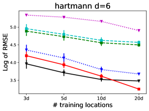
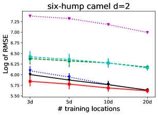
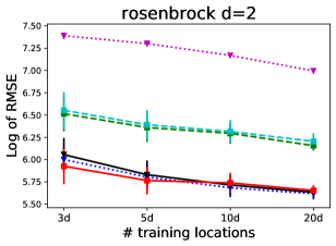
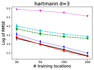
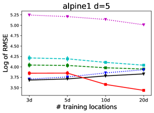
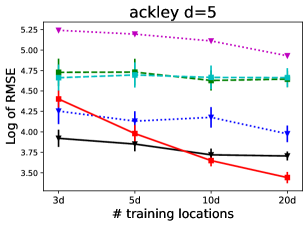
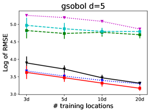
Figure 3: Exploiting external knowledge about f+superscript𝑓f^{+} and fsuperscript𝑓f^{-} leads to better gp posterior sampling.

Given π(gm)=𝒩([gm,gm+][f,f+],diag[η2,η+2])𝜋subscript𝑔𝑚𝒩conditionalsubscriptsuperscript𝑔𝑚subscriptsuperscript𝑔𝑚superscript𝑓superscript𝑓diagsubscriptsuperscript𝜂2subscriptsuperscript𝜂2\pi(g_{m})=\mathcal{N}\big{(}\left[g^{-}_{m},g^{+}_{m}\right]\mid\left[f^{-},f^{+}\right],\text{diag}[\eta^{2}_{-},\eta^{2}_{+}]\big{)} in Eq. (4), we want to quantify the influence of a new data point {𝐱,y𝐱}𝐱subscript𝑦𝐱\{\mathbf{x},y_{\mathbf{x}}\} on a given gp posterior sample. We write the likelihood with and without the presence of 𝐱𝐱\mathbf{x}.

p(gm+,𝐱m+Λ)𝑝superscriptsubscript𝑔𝑚conditionalsuperscriptsubscript𝐱𝑚Λ\displaystyle p\left(g_{m}^{+},\mathbf{x}_{m}^{+}\mid\Lambda\right) =p(gm+𝐱m+,Λ)p(𝐱m+Λ)absent𝑝conditionalsuperscriptsubscript𝑔𝑚superscriptsubscript𝐱𝑚Λ𝑝conditionalsuperscriptsubscript𝐱𝑚Λ\displaystyle={\color[rgb]{0,0,1}\definecolor[named]{pgfstrokecolor}{rgb}{0,0,1}p\left(g_{m}^{+}\mid\mathbf{x}_{m}^{+},\Lambda\right)}{\color[rgb]{1,.5,0}\definecolor[named]{pgfstrokecolor}{rgb}{1,.5,0}p\left(\mathbf{x}_{m}^{+}\mid\Lambda\right)} (10)
π(gm)𝒩(gm(𝐱m+)μ(𝐱m+),σ2(𝐱m+))absent𝜋subscript𝑔𝑚𝒩conditionalsubscript𝑔𝑚subscriptsuperscript𝐱𝑚𝜇subscriptsuperscript𝐱𝑚superscript𝜎2superscriptsubscript𝐱𝑚\displaystyle\approx{\color[rgb]{0,0,1}\definecolor[named]{pgfstrokecolor}{rgb}{0,0,1}\pi(g_{m})}{\color[rgb]{1,.5,0}\definecolor[named]{pgfstrokecolor}{rgb}{1,.5,0}\mathcal{N}\left(g_{m}(\mathbf{x}^{+}_{m})\mid\mu(\mathbf{x}^{+}_{m}),\sigma^{2}(\mathbf{x}_{m}^{+})\right)}
p(gm+,𝐱m+y𝐱,Λ)𝑝superscriptsubscript𝑔𝑚conditionalsuperscriptsubscript𝐱𝑚subscript𝑦𝐱Λ\displaystyle p\left(g_{m}^{+},\mathbf{x}_{m}^{+}\mid y_{{\color[rgb]{1,0,0}\definecolor[named]{pgfstrokecolor}{rgb}{1,0,0}\mathbf{x}}},\Lambda\right) =p(gm+𝐱m+,y𝐱,Λ)p(𝐱m+y𝐱,Λ)absent𝑝conditionalsuperscriptsubscript𝑔𝑚superscriptsubscript𝐱𝑚subscript𝑦𝐱Λ𝑝conditionalsuperscriptsubscript𝐱𝑚subscript𝑦𝐱Λ\displaystyle=p\left(g_{m}^{+}\mid\mathbf{x}_{m}^{+},y_{{\color[rgb]{1,0,0}\definecolor[named]{pgfstrokecolor}{rgb}{1,0,0}\mathbf{x}}},\Lambda\right)p\left(\mathbf{x}_{m}^{+}\mid y_{{\color[rgb]{1,0,0}\definecolor[named]{pgfstrokecolor}{rgb}{1,0,0}\mathbf{x}}},\Lambda\right) (11)
π(gm)𝒩(gm(𝐱m+)μ𝐱(𝐱m+),σ𝐱2(𝐱m+))absent𝜋subscript𝑔𝑚𝒩conditionalsubscript𝑔𝑚subscriptsuperscript𝐱𝑚subscript𝜇𝐱subscriptsuperscript𝐱𝑚subscriptsuperscript𝜎2𝐱superscriptsubscript𝐱𝑚\displaystyle\approx\pi(g_{m})\mathcal{N}\left(g_{m}(\mathbf{x}^{+}_{m})\mid\mu_{{\color[rgb]{1,0,0}\definecolor[named]{pgfstrokecolor}{rgb}{1,0,0}\mathbf{x}}}(\mathbf{x}^{+}_{m}),\sigma^{2}_{{\color[rgb]{1,0,0}\definecolor[named]{pgfstrokecolor}{rgb}{1,0,0}\mathbf{x}}}(\mathbf{x}_{m}^{+})\right)

where μ𝐱(𝐱m+)subscript𝜇𝐱superscriptsubscript𝐱𝑚\mu_{\mathbf{x}}(\mathbf{x}_{m}^{+}), μ(𝐱m+)𝜇superscriptsubscript𝐱𝑚\mu(\mathbf{x}_{m}^{+}), σ𝐱2(𝐱m+)subscriptsuperscript𝜎2𝐱superscriptsubscript𝐱𝑚\sigma^{2}_{\mathbf{x}}(\mathbf{x}_{m}^{+}), and σ2(𝐱m+)superscript𝜎2superscriptsubscript𝐱𝑚\sigma^{2}(\mathbf{x}_{m}^{+})222 we use a subscript σ𝐱()subscript𝜎𝐱\sigma_{\mathbf{x}}(\cdot) to indicate the inclusion of 𝐱𝐱\mathbf{x}. are the gp posterior predictive means and variances at 𝐱m+superscriptsubscript𝐱𝑚\mathbf{x}_{m}^{+} with and without the inclusion of 𝐱𝐱\mathbf{x}. These predictive quantities are defined in Eqs. (6) and (7). Plugging Eqs. (10) and (11) into Eq. (9), we obtain the final form of αbes(𝐱)superscript𝛼bes𝐱\alpha^{\lx@glossaries@gls@link{acronym}{BES}{\leavevmode\textsc{bes}}}(\mathbf{x}).

In Eq. (10), the likelihood p(𝐱m+Λ)𝑝conditionalsuperscriptsubscript𝐱𝑚Λ{\color[rgb]{1,.5,0}\definecolor[named]{pgfstrokecolor}{rgb}{1,.5,0}p\left(\mathbf{x}_{m}^{+}\mid\Lambda\right)} can be defined to a prior knowledge about the input 𝐱m+subscriptsuperscript𝐱𝑚\mathbf{x}^{+}_{m} if available, such as Li et al., (2020); Souza et al., (2021). Instead of using uniform prior, we can have better estimation by using the GP predictive mean μ(𝐱m+)𝜇subscriptsuperscript𝐱𝑚\mu(\mathbf{x}^{+}_{m}) and variance σ2(𝐱m+)superscript𝜎2superscriptsubscript𝐱𝑚\sigma^{2}(\mathbf{x}_{m}^{+}) available to quantify the likelihood of the location of interest 𝐱m+subscriptsuperscript𝐱𝑚\mathbf{x}^{+}_{m} being the optimum (given the data).

Without knowing the true output at a test location 𝐱𝐱\mathbf{x}, we can simplify the gp predictive mean μ𝐱(𝐱m+)μ(𝐱m+)subscript𝜇𝐱subscriptsuperscript𝐱𝑚𝜇subscriptsuperscript𝐱𝑚\mu_{\mathbf{x}}(\mathbf{x}^{+}_{m})\approx\mu(\mathbf{x}^{+}_{m}). This simplification saves computation cost for updating the gp predictive mean at each considered location 𝐱𝐱\mathbf{x}.

The term π(gm)𝜋subscript𝑔𝑚\pi(g_{m}) in Eq. (11) will be retained when plugging into Eq. (9). Thus, π(gm)𝜋subscript𝑔𝑚\pi(g_{m}) will remove any gp sample which does not follow our bounded constraints. As a result, our decision only gains information about the ‘good’ samples. In Appendix C.3, we provide an ablation study by accepting all samples (without weighting step), which drops the performance significantly.

Explainable decision.

The point selected by Eq. (9) will gain the maximum information about the posterior samples. Our decision can be interpretable in each single term. The acquisition function value in Eq. (9) is high when the density p(gm+,𝐱m+y𝐱,Λ)p(gm+,𝐱m+Λ)𝑝superscriptsubscript𝑔𝑚conditionalsuperscriptsubscript𝐱𝑚subscript𝑦𝐱Λ𝑝superscriptsubscript𝑔𝑚conditionalsuperscriptsubscript𝐱𝑚Λ\frac{p\left(g_{m}^{+},\mathbf{x}_{m}^{+}\mid y_{\mathbf{x}},\Lambda\right)}{p\left(g_{m}^{+},\mathbf{x}_{m}^{+}\mid\Lambda\right)} and p(gm+,𝐱m+y𝐱,Λ)𝑝superscriptsubscript𝑔𝑚conditionalsuperscriptsubscript𝐱𝑚subscript𝑦𝐱Λp\left(g_{m}^{+},\mathbf{x}_{m}^{+}\mid y_{\mathbf{x}},\Lambda\right) are high, defined in Eqs. (10) and (11). The first term p(gm+,𝐱m+y𝐱,Λ)p(gm+,𝐱m+Λ)𝒩(gm+μ(𝐱m+),[σ𝐱2(𝐱m+)1σ2(𝐱m+)1]1)proportional-to𝑝superscriptsubscript𝑔𝑚conditionalsuperscriptsubscript𝐱𝑚subscript𝑦𝐱Λ𝑝superscriptsubscript𝑔𝑚conditionalsuperscriptsubscript𝐱𝑚Λ𝒩conditionalsuperscriptsubscript𝑔𝑚𝜇subscriptsuperscript𝐱𝑚superscriptdelimited-[]subscriptsuperscript𝜎2𝐱superscriptsuperscriptsubscript𝐱𝑚1superscript𝜎2superscriptsuperscriptsubscript𝐱𝑚11\frac{p\left(g_{m}^{+},\mathbf{x}_{m}^{+}\mid y_{\mathbf{x}},\Lambda\right)}{p\left(g_{m}^{+},\mathbf{x}_{m}^{+}\mid\Lambda\right)}\propto\mathcal{N}(g_{m}^{+}\mid\mu(\mathbf{x}^{+}_{m}),\left[\sigma^{2}_{\mathbf{x}}(\mathbf{x}_{m}^{+})^{-1}-\sigma^{2}(\mathbf{x}_{m}^{+})^{-1}\right]^{-1}) is high when σ𝐱2(𝐱m+)σ2(𝐱m+)much-less-thansubscriptsuperscript𝜎2𝐱superscriptsubscript𝐱𝑚superscript𝜎2superscriptsubscript𝐱𝑚\sigma^{2}_{\mathbf{x}}(\mathbf{x}_{m}^{+})\ll\sigma^{2}(\mathbf{x}_{m}^{+}) given that 𝔼[gm+]=μ(𝐱m+)𝔼delimited-[]subscriptsuperscript𝑔𝑚𝜇subscriptsuperscript𝐱𝑚\mathbb{E}[g^{+}_{m}]=\mu(\mathbf{x}^{+}_{m}). To reduce this predictive uncertainty of σ𝐱2(𝐱m+)subscriptsuperscript𝜎2𝐱subscriptsuperscript𝐱𝑚\sigma^{2}_{\mathbf{x}}(\mathbf{x}^{+}_{m}), our acquisition function encourages to place a point 𝐱𝐱\mathbf{x} at the perceived optimum location 𝐱m+subscriptsuperscript𝐱𝑚\mathbf{x}^{+}_{m}. Similarly, the second term p(gm+,𝐱m+y𝐱,Λ)𝑝superscriptsubscript𝑔𝑚conditionalsuperscriptsubscript𝐱𝑚subscript𝑦𝐱Λp\left(g_{m}^{+},\mathbf{x}_{m}^{+}\mid y_{\mathbf{x}},\Lambda\right) takes high value when π(gm)𝜋subscript𝑔𝑚\pi(g_{m}) is high and σ𝐱2(𝐱m+)subscriptsuperscript𝜎2𝐱superscriptsubscript𝐱𝑚\sigma^{2}_{\mathbf{x}}(\mathbf{x}_{m}^{+}) is small. This encourages (i) the sampled gp has the maximum value gm+superscriptsubscript𝑔𝑚g_{m}^{+} consistent with f+superscript𝑓f^{+} and (ii) taking a location at 𝐱m+superscriptsubscript𝐱𝑚\mathbf{x}_{m}^{+}. We refer to Appendix A for the illustration of the αbessuperscript𝛼bes\alpha^{\lx@glossaries@gls@link{acronym}{BES}{\leavevmode\textsc{bes}}} and B.2 for the implementation discussion. We summarize all steps for computing bes in Algorithm 2.

5 Experiments

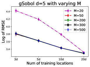
We demonstrate the two claims in exploiting the knowledge of f+superscript𝑓f^{+}and fsuperscript𝑓f^{-} for improving gp posterior sampling and bo. We also perform ablation studies by varying the misspecified levels of such bounds for each setting. All experiments are averaged over 303030 independent runs, the number of gp samples M=200𝑀200M=200,333The ablation study with different choices of M{20,50,200,300,500}𝑀2050200300500M\in\{20,50,200,300,500\} is available in Appendix C.1 η+2=0.02dsubscriptsuperscript𝜂20.02𝑑\eta^{2}_{+}=0.02d and η2=0.5dsubscriptsuperscript𝜂20.5𝑑\eta^{2}_{-}=0.5d where d𝑑d is the input dimension. The dimension of random Fourier features is set to default as l=100𝑙100l=100. We normalize the input 𝐱[0,1]d𝐱superscript01𝑑\mathbf{x}\in[0,1]^{d} and standardize the output y𝒩(0,1)similar-to𝑦𝒩01y\sim\mathcal{N}(0,1) for robustness. We follow the common practice in optimizing gp hyperparameter by maximizing the gp log marginal likelihood (Rasmussen and Williams,, 2006). We refer to the appendix for additional experiments, illustrations, and ablation studies. We attach the Python source code in the submission and will release publicly in the final version.

srgp vs gp.

The key advantage of srgp is that we can generate ‘good’ samples more often than using a standard gp in Section 3.1. We demonstrate this benefit in Fig. 1 showing that srgp with weighting (or w-srgp) outperforms w-gp. The results are more significant in higher dimensional functions where the w-gp cannot get a single sample accepted for alpine1 in 5d5𝑑5d using M=200𝑀200M=200.

Refer to caption
Refer to caption
Refer to caption
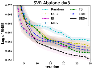
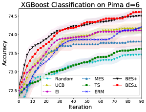
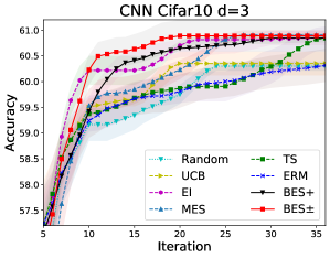
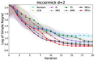
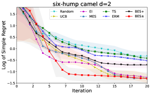
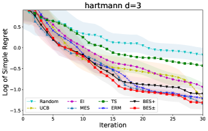
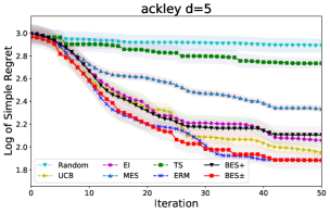
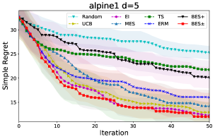
Figure 4: Machine learning hyperparameter tuning tasks. Exploiting the knowledge about optimum values will lead to better optimisation performance. bes ±plus-or-minus\pm (with f+superscript𝑓f^{+} and fsuperscript𝑓f^{-}) performs the best. In svr setting, we only use f+superscript𝑓f^{+} while we have ultilized both f+superscript𝑓f^{+} and fsuperscript𝑓f^{-} for xgboost and cnn.
Refer to caption
Figure 5: Our method can improve the performance of gp posterior sampling without using f+superscript𝑓f^{+} or fsuperscript𝑓f^{-} (Wilson et al.,, 2020) (black dash line) under misspecification of f+,fsuperscript𝑓superscript𝑓f^{+},f^{-}. The gap is more significant given fewer training observations. The plot is using Forrester function. See the Appendix Fig. 14 for more results.

Improving gp posterior sampling.

A set of training locations 𝐗trainU[0,1]Ntrain×dsimilar-tosubscript𝐗train𝑈superscript01subscript𝑁train𝑑\mathbf{X}_{\textrm{train}}\sim U[0,1]^{N_{\textrm{train}}\times d} is randomly generated and corresponding outputs 𝐲train=f(𝐗train)subscript𝐲train𝑓subscript𝐗train\mathbf{y}_{\textrm{train}}=f(\mathbf{X}_{\textrm{train}}) are subsequently observed. We construct a gp given {𝐗train,𝐲train}subscript𝐗trainsubscript𝐲train\left\{\mathbf{X}_{\textrm{train}},\mathbf{y}_{\textrm{train}}\right\} and draw M=200𝑀200M=200 gp posterior samples for each sampling scheme. Due to the trade-off between the number of accepted gp samples versus the sampling quality for these methods with exploiting f+superscript𝑓f^{+} and flimit-from𝑓f-, we rank and select the same (M=100superscript𝑀100M^{\prime}=100) number of posterior samples from the initial set of M=200𝑀200M=200 samples above. These samples are used to compute the rmse error against the true f()𝑓f(\cdot).

We vary the number of training locations Ntrain={3d,5d,10d,20d}subscript𝑁train3𝑑5𝑑10𝑑20𝑑N_{\textrm{train}}=\{3d,5d,10d,20d\} and report the results in Fig. 3 which suggest that increasing the number of training observations will reduce the error for all sampling schemes. More importantly, incorporating the knowledge about f+superscript𝑓f^{+} and fsuperscript𝑓f^{-} will significantly improve the gp posterior sampling performance. Furthermore, using both f+superscript𝑓f^{+} and fsuperscript𝑓f^{-} results in better performance than using f+superscript𝑓f^{+} alone. Our approach surpasses the standard gp sampling (Wilson et al.,, 2020), which does not use the bound information, by a wide margin. The logistic and sigmoid transformations making use of the bounds are generally better than the standard GP, but are inferior to our proposed methods. We present further details and visualization of these transformations in Appendix B.1.

Improving Bayesian optimization.

We next present a bo task. We follow a popular evaluation criterion in information theoretic approaches (Hennig and Schuler,, 2012; Hernández-Lobato et al.,, 2014) that selects the inferred argmax of the function for evaluation, i.e. 𝐱~T=argmax𝐱𝒳μT(𝐱DT)subscript~𝐱𝑇subscript𝐱𝒳subscript𝜇𝑇conditional𝐱subscript𝐷𝑇\widetilde{\mathbf{x}}_{T}=\arg\max_{\mathbf{x}\in\mathcal{X}}\mu_{T}\left(\mathbf{x}\mid D_{T}\right). The number of bo iterations is 10d10𝑑10d, initialized by d𝑑d observations randomly where d𝑑d is the number of input dimension. We compare our model with standard bo methods which do not use f+superscript𝑓f^{+} and fsuperscript𝑓f^{-}, including gp-ucb (Srinivas et al.,, 2010), expected improvement (ei) (Mockus et al.,, 1978), max-value entropy search (mes) (Wang and Jegelka,, 2017) and Thompson sampling (ts). We compare with erm (Nguyen and Osborne,, 2020), which can make use of either f+superscript𝑓f^{+} or fsuperscript𝑓f^{-}, but not both of them. We compare the performance using popular benchmark functions and machine learning hyperparameter tunings including support vector regression (Smola and Vapnik,, 1997) on Abalone using root mean squared error (RMSE) as the main metric, xgboost (Chen and Guestrin,, 2016) classification on Pima Indians diabetes, and a cnn (LeCun and Bengio,, 1995) on cifar10. We refer to Appendix C.3 for studying a variant of bes where π(gm)=1M𝜋subscript𝑔𝑚1𝑀\pi(g_{m})=\frac{1}{M} is set uniformly and Appendix D.2 for additional experiments.
Refer to caption
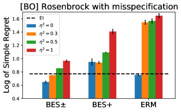
Figure 6: Our bes is more robust than erm in dealing with misspecification.

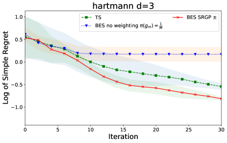
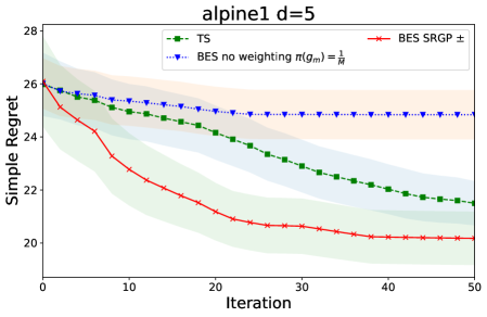
bes ±plus-or-minus\pm is an abbreviation for bes using both f+superscript𝑓f^{+} and fsuperscript𝑓f^{-} while bes ++ uses f+superscript𝑓f^{+} alone. We show in Fig. 4 that exploiting the optimum knowledge in our bes and erm should perform competitively. Notably, our bes often achieves high performances at the earlier stage of the optimization process where we do not have much information to infer the underlying function. Therefore, utilizing f+,fsuperscript𝑓superscript𝑓f^{+},f^{-} will bring significant benefits at the earlier stage that the existing approaches are unable to exploit. We note that when f+superscript𝑓f^{+} and fsuperscript𝑓f^{-} are available, the erm is unable to exploit both.

Misspecifying f+superscript𝑓f^{+} and fsuperscript𝑓f^{-}.

We perform ablation studies over different misspecified levels of the optimum values via η2:=η+2=η2{0,1,3,5}assignsuperscript𝜂2subscriptsuperscript𝜂2subscriptsuperscript𝜂20135\eta^{2}:=\eta^{2}_{+}=\eta^{2}_{-}\in\{0,1,3,5\} for gp sampling and η2{0,0.3,0.5,1}superscript𝜂200.30.51\eta^{2}\in\{0,0.3,0.5,1\} for bo. Using the benchmark functions, we have access to the true values of maxf()𝑓\max f(\cdot) and minf()𝑓\min f(\cdot). Thus, the misspecified value is set as f+=maxf()±η+2superscript𝑓plus-or-minus𝑓subscriptsuperscript𝜂2f^{+}=\max f(\cdot)\pm\eta^{2}_{+} where ±plus-or-minus\pm is randomly selected by a Bernoulli random variable. fsuperscript𝑓f^{-} is specified analogously.

For a meaningful study, we consider these values after standardizing the output space y𝒩(0,1)similar-to𝑦𝒩01y\sim\mathcal{N}(0,1). This means that when η2=1superscript𝜂21\eta^{2}=1, the gap between the true maxf()𝑓\max f(\cdot) and the specified f+superscript𝑓f^{+} is one standard deviation of f()𝑓f(\cdot). We present further experimental results in the Appendix Fig. 14.

When η21superscript𝜂21\eta^{2}\leq 1, the performance of gp posterior sampling in Fig. 5 is much better than Wilson et al., (2020) in all cases and when η25superscript𝜂25\eta^{2}\leq 5 our model is still better in a few cases. Relaxing η2superscript𝜂2\eta^{2}\rightarrow\infty will let the performance of w-gp reduce to the case of Wilson et al., (2020) while the performance of w-srgp will slightly suffer because the transformation depends on η+2subscriptsuperscript𝜂2\eta^{2}_{+}. Thus, we suggest to use our weighting srgp when the misspecification is such that η21superscript𝜂21\eta^{2}\leq 1, one standard deviation of f()𝑓f(\cdot), and use w-gp otherwise.

We study misspecifying f+superscript𝑓f^{+} and fsuperscript𝑓f^{-} for bo. In Fig. 6, our bes performs competitively the best, especially when η20.3superscript𝜂20.3\eta^{2}\leq 0.3 in all cases. The information gain strategy in bes is more noise-resilient in dealing with misspecification than erm. Especially if we underspecify f+superscript𝑓f^{+}, the performance of erm will significantly drop as shown in Nguyen and Osborne, (2020), while our bes can tolerate better. Utilizing both information about f+superscript𝑓f^{+} and fsuperscript𝑓f^{-} will help to cope with misspecification better than using f+superscript𝑓f^{+} alone.

Refer to caption
Figure 7: We specify f+superscript𝑓f^{+} to different values and set fsuperscript𝑓f^{-} fixed in xgboost. The performance is better when f+superscript𝑓f^{+} is set closer to the true value 0.745absent0.745\approx 0.745.

In Fig. 7, we vary the values of f+superscript𝑓f^{+} within [0.7,0.9]0.70.9[0.7,0.9] and fix f=0.65superscript𝑓0.65f^{-}=0.65 in the xgboost classification problem where we do not know the true value for these bounds. The result indicates that the best performance for bes is achieved when f+superscript𝑓f^{+} is set close to 0.745absent0.745\approx 0.745, which is likely the true (but unknown) upper bound. Our bes with misspecifying f+[0.73,0.75]superscript𝑓0.730.75f^{+}\in[0.73,0.75] still performs generally better than ei.

6 Conclusion, limitations and future work

Conclusion.

We have presented a new setting and approaches for exploiting the upper and lower bounds available for some black-box functions. We exploit these bounds for improving the performance of gp posterior sampling and bo. The resulting gp posterior sampling approach has tighter sample variance bounds than existing methods. Our approaches can be used as a plugin extension to existing distributed and asynchronous Thompson sampling as well as sparse gp models.

Comparisons with erm (Nguyen and Osborne,, 2020).

Our key advantages against erm is as follows. First, our approach can handle the information about both the max and min of f()𝑓f(\cdot) while the setting in erm can only handle one of them. Second, our approach is more widely applicable in taking the optimum values which can be loosely specified while erm expects to observe the precise value. Particularly, erm will perform poorly if users underspecified the true value of max𝐱f(𝐱)subscript𝐱𝑓𝐱\max_{\mathbf{x}}f(\mathbf{x}). Third, our approach is useful for both gp posterior sampling and bo settings while the one suggested by Nguyen and Osborne, (2020) is limited to bo.

Limitations.

While we believe the results above are insightful, there are a number of limitations one needs to be aware of. First, our bes relies on the gp posterior samples to make a decision. There will be some iterations where none of the gp samples stays within the approximate bounds, such as when M𝑀M is small or the available data is biased to represent f()𝑓f(\cdot). Whenever this happens, our bes may be not applicable; instead we can simply perform ei (Jones et al.,, 1998) for this iteration. We found this simple trick with ei works well empirically and illustrate it in Appendix C.2. Second, we acknowledge the challenge when the bounds are heavily mis-specified, where such knowledge about the bounds can be less beneficial. Thus, the results in Fig. 7 suggest that if our loose bounds are defined more than η2>0.3superscript𝜂20.3\eta^{2}>0.3, it may be better to use existing acquisition functions, such as ei, without using the external knowledge.

Future work can extend the model to optimize multiple objectives simultaneously, each of which comes with loose upper and lower bounds. Using such bounds, other future works can be to improve parallel Thompson sampling (Hernández-Lobato et al.,, 2017; Kirthevasan et al.,, 2018) or used jointly with other signals, such as monotonicity, for the best performance in the low data regime. Another direction for improving the sample efficiency is to consider important sampling on the space of random Fourier feature while we expect the high dimensional challenge.

Bibliography

  • Aster et al., (2018) Aster, R. C., Borchers, B., and Thurber, C. H. (2018). Parameter Estimation and Inverse Problems. Elsevier.
  • Bertero and Boccacci, (2020) Bertero, M. and Boccacci, P. (2020). Introduction to inverse problems in imaging. CRC press.
  • Brochu et al., (2010) Brochu, E., Cora, V. M., and De Freitas, N. (2010). A tutorial on Bayesian optimization of expensive cost functions, with application to active user modeling and hierarchical reinforcement learning. arXiv preprint arXiv:1012.2599.
  • Chen and Guestrin, (2016) Chen, T. and Guestrin, C. (2016). Xgboost: A scalable tree boosting system. In Proceedings of the 22nd ACM SigKDD International Conference on Knowledge Discovery and Data Mining, pages 785–794. ACM.
  • Chiles and Delfiner, (2009) Chiles, J.-P. and Delfiner, P. (2009). Geostatistics: Modeling Spatial Uncertainty, volume 497. John Wiley & Sons.
  • Deisenroth and Rasmussen, (2011) Deisenroth, M. P. and Rasmussen, C. E. (2011). PILCO: a model-based and data-efficient approach to policy search. In Proceedings of the International Conference on Machine Learning, pages 465–472.
  • Doucet, (2010) Doucet, A. (2010). A note on efficient conditional simulation of Gaussian distributions. Department of Computer Science and Statistics, University of British Columbia, 4.
  • Gunter et al., (2014) Gunter, T., Osborne, M. A., Garnett, R., Hennig, P., and Roberts, S. J. (2014). Sampling for inference in probabilistic models with fast Bayesian quadrature. In Advances in Neural Information Processing Systems, pages 2789–2797.
  • György and Kocsis, (2011) György, A. and Kocsis, L. (2011). Efficient multi-start strategies for local search algorithms. Journal of Artificial Intelligence Research, 41:407–444.
  • Hennig and Schuler, (2012) Hennig, P. and Schuler, C. J. (2012). Entropy search for information-efficient global optimization. Journal of Machine Learning Research, 13:1809–1837.
  • Hernández-Lobato et al., (2014) Hernández-Lobato, J. M., Hoffman, M. W., and Ghahramani, Z. (2014). Predictive entropy search for efficient global optimization of black-box functions. In Advances in Neural Information Processing Systems, pages 918–926.
  • Hernández-Lobato et al., (2017) Hernández-Lobato, J. M., Requeima, J., Pyzer-Knapp, E. O., and Aspuru-Guzik, A. (2017). Parallel and distributed Thompson sampling for large-scale accelerated exploration of chemical space. In International Conference on Machine Learning, pages 1470–1479.
  • Jones et al., (1998) Jones, D. R., Schonlau, M., and Welch, W. J. (1998). Efficient global optimization of expensive black-box functions. Journal of Global Optimization, 13(4):455–492.
  • Journel and Huijbregts, (1978) Journel, A. G. and Huijbregts, C. J. (1978). Mining Geostatistics, volume 600. Academic Press London.
  • Kirthevasan et al., (2018) Kirthevasan, K., Akshay, K., Jeff, S., and Barnabas, P. (2018). Parallelised Bayesian optimisation via Thompson sampling. In AISTATS.
  • Krizhevsky et al., (2012) Krizhevsky, A., Sutskever, I., and Hinton, G. E. (2012). Imagenet classification with deep convolutional neural networks. In Advances in Neural Information Processing Systems, pages 1097–1105.
  • LeCun and Bengio, (1995) LeCun, Y. and Bengio, Y. (1995). Convolutional networks for images, speech, and time series. The handbook of brain theory and neural networks, 3361(10):1995.
  • Li et al., (2020) Li, C., Gupta, S., Rana, S., Nguyen, V., Robles-Kelly, A., and Venkatesh, S. (2020). Incorporating expert prior knowledge into experimental design via posterior sampling. arXiv preprint arXiv:2002.11256.
  • Li et al., (2018) Li, C., Santu, R., Gupta, S., Nguyen, V., Venkatesh, S., Sutti, A., Leal, D. R. D. C., Slezak, T., Height, M., Mohammed, M., and Gibson, I. (2018). Accelerating experimental design by incorporating experimenter hunches. In International Conference on Data Mining, pages 257–266.
  • Mockus et al., (1978) Mockus, J., Tiesis, V., and Zilinskas, A. (1978). The application of Bayesian methods for seeking the extremum. Towards Global Optimization, 2(117-129):2.
  • Mosegaard and Tarantola, (1995) Mosegaard, K. and Tarantola, A. (1995). Monte carlo sampling of solutions to inverse problems. Journal of Geophysical Research: Solid Earth, 100(B7):12431–12447.
  • Nguyen et al., (2019) Nguyen, V., Gupta, S., Rana, S., Thai, M., Li, C., and Venkatesh, S. (2019). Efficient Bayesian optimization for uncertainty reduction over perceived optima locations. In International Conference on Data Mining.
  • Nguyen and Osborne, (2020) Nguyen, V. and Osborne, M. A. (2020). Knowing the what but not the where in Bayesian optimization. In International Conference on Machine Learning, pages 7317–7326.
  • Parker-Holder et al., (2020) Parker-Holder, J., Nguyen, V., and Roberts, S. J. (2020). Provably efficient online hyperparameter optimization with population-based bandits. Advances in Neural Information Processing Systems.
  • Perrone et al., (2019) Perrone, V., Shen, H., Seeger, M. W., Archambeau, C., and Jenatton, R. (2019). Learning search spaces for Bayesian optimization: Another view of hyperparameter transfer learning. In Advances in Neural Information Processing Systems, pages 12771–12781.
  • Popoviciu, (1935) Popoviciu, T. (1935). Sur les équations algébriques ayant toutes leurs racines réelles. Mathematica, 9:129–145.
  • Rahimi and Recht, (2007) Rahimi, A. and Recht, B. (2007). Random features for large-scale kernel machines. In Advances in Neural Information Processing Systems, pages 1177–1184.
  • Rasmussen and Williams, (2006) Rasmussen, C. E. and Williams, C. K. I. (2006). Gaussian Processes for Machine Learning. MIT Prees.
  • Richardson et al., (2017) Richardson, R. R., Osborne, M. A., and Howey, D. A. (2017). Gaussian process regression for forecasting battery state of health. Journal of Power Sources, 357:209–219.
  • Riihimäki and Vehtari, (2010) Riihimäki, J. and Vehtari, A. (2010). Gaussian processes with monotonicity information. In International Conference on Artificial Intelligence and Statistics, pages 645–652.
  • Ru et al., (2018) Ru, B., McLeod, M., Granziol, D., and Osborne, M. A. (2018). Fast information-theoretic Bayesian optimisation. In International Conference on Machine Learning, pages 4381–4389.
  • Russo et al., (2018) Russo, D. J., Van Roy, B., Kazerouni, A., Osband, I., and Wen, Z. (2018). A tutorial on Thompsonsampling. Foundations and Trends® in Machine Learning, 11(1):1–96.
  • Shahriari et al., (2016) Shahriari, B., Swersky, K., Wang, Z., Adams, R. P., and de Freitas, N. (2016). Taking the human out of the loop: A review of Bayesian optimization. Proceedings of the IEEE, 104(1):148–175.
  • Smola and Vapnik, (1997) Smola, A. and Vapnik, V. (1997). Support vector regression machines. Advances in Neural Information Processing Systems, 9:155–161.
  • Souza et al., (2021) Souza, A., Nardi, L., Oliveira, L. B., Olukotun, K., Lindauer, M., and Hutter, F. (2021). Bayesian optimization with a prior for the optimum. In Joint European Conference on Machine Learning and Knowledge Discovery in Databases, pages 265–296. Springer.
  • Srinivas et al., (2010) Srinivas, N., Krause, A., Kakade, S., and Seeger, M. (2010). Gaussian process optimization in the bandit setting: No regret and experimental design. In International Conference on Machine Learning, pages 1015–1022.
  • Thompson, (1933) Thompson, W. R. (1933). On the likelihood that one unknown probability exceeds another in view of the evidence of two samples. Biometrika, 25(3/4):285–294.
  • Wang and Jegelka, (2017) Wang, Z. and Jegelka, S. (2017). Max-value entropy search for efficient Bayesian optimization. In International Conference on Machine Learning, pages 3627–3635.
  • Wilson et al., (2020) Wilson, J. T., Borovitskiy, V., Terenin, A., Mostowsky, P., and Deisenroth, M. P. (2020). Efficiently sampling functions from Gaussian process posteriors. In International Conference on Machine Learning, pages 10292–10302.
  • Wilson et al., (2021) Wilson, J. T., Borovitskiy, V., Terenin, A., Mostowsky, P., and Deisenroth, M. P. (2021). Pathwise conditioning of gaussian processes. Journal of Machine Learning Research, 22(105):1–47.
Refer to caption
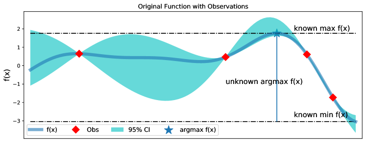
(a) We have a black-box function f(𝐱)𝑓𝐱f(\mathbf{x}) including four observations (red dots), the maximum value fsuperscript𝑓f^{-} and minimum value fsuperscript𝑓f^{-}. The goal is to find the unknown maximum location argmaxf(𝐱)𝑓𝐱\arg\max f(\mathbf{x}).
Refer to caption
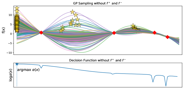
(b) Top: gp posterior sampling pbasesubscript𝑝basep_{\textrm{base}} without the knowledge about f+superscript𝑓f^{+} and fsuperscript𝑓f^{-}. Bottom: the decision function will select the left corner which is not the correct maximum location.
Refer to caption
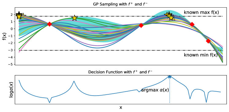
(c) Top: gp posterior sampling π(gm)𝜋subscript𝑔𝑚\pi(g_{m}) guided by the f+superscript𝑓f^{+} and fsuperscript𝑓f^{-}. Bottom: our decision selects the next point for evaluation correctly as the unknown maximum location, i.e., argmaxαbes(𝐱)=argmaxf(𝐱)superscript𝛼bes𝐱𝑓𝐱\arg\max\alpha^{\textrm{\lx@glossaries@gls@link{acronym}{BES}{\leavevmode{bes}}}}(\mathbf{x})=\arg\max f(\mathbf{x}).
Figure 8: Illustrating the bes. Top: a black-box function f(𝐱)𝑓𝐱f(\mathbf{x}) and four observations (red dots). Middle: pbasesubscript𝑝basep_{\textrm{base}} as a gp and the decision without the weighting π(gm)𝜋subscript𝑔𝑚\pi(g_{m}). Bottom: pbasesubscript𝑝basep_{\textrm{base}} as a srgp and the decision with the weighting π(gm)𝜋subscript𝑔𝑚\pi(g_{m}) .

Appendix A Illustration of Bounded Entropy Search (bes) Decision Function

We first illustrate the decision function of bes given the knowledge of f+=maxf(𝐱)+𝒩(0,η+2)superscript𝑓𝑓𝐱𝒩0subscriptsuperscript𝜂2f^{+}=\max f(\mathbf{x})+\mathcal{N}(0,\eta^{2}_{+}) and f=minf(𝐱)+𝒩(0,η2)superscript𝑓𝑓𝐱𝒩0subscriptsuperscript𝜂2f^{-}=\min f(\mathbf{x})+\mathcal{N}(0,\eta^{2}_{-}) in Fig. 8. Given limited observations in Fig. 8a, it may be difficult to infer the unknown optimum location argmaxf(𝐱)𝑓𝐱\arg\max f(\mathbf{x}). However, we can utilize the information about the upper bound and lower bound to better identify this location of interest. In particular, we show that incorporating f+superscript𝑓f^{+} and fsuperscript𝑓f^{-} can help to identify correctly the unknown maximum location in Fig. 8c while we may fail without such extra knowledge as shown in Fig. 8b.

Appendix B Further Technical Details

B.1 Transformation by sinusoidal and sigmoid
Refer to caption
Refer to caption
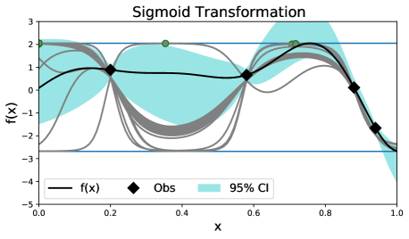
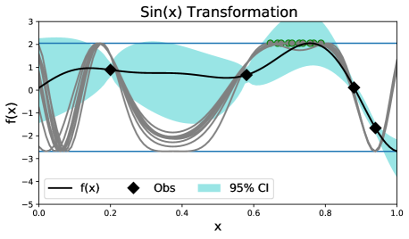
Figure 9: gp posterior sampling with f+,fsuperscript𝑓superscript𝑓f^{+},f^{-} transformations by sinusoidal and sigmoid functions. They both result in not good estimation although they satisfy the bounded constraints. The major issue with these transformations is that the gp samples are stretched out too much at the two tails f+superscript𝑓f^{+} and flimit-from𝑓f-.

We present two other ways to transform the gp posterior samples by incorporating the knowledge about f+superscript𝑓f^{+} and fsuperscript𝑓f^{-}. We utilize the sin wave and sigmoid transformations. For such transformations, we define a forward function to compute f(𝐱)𝑓𝐱f(\mathbf{x}) given h(𝐱)𝐱h(\mathbf{x}) which is constrained by either arcsin\arcsin or log\log. Then, we define a reverse function to compute h(𝐱)𝐱h(\mathbf{x}) given f(𝐱)𝑓𝐱f(\mathbf{x}). These forward and reverse functions are summarized below:

  • Using sinusoidal transformation: we define f(𝐱)ff+f=12sin[h(𝐱)]+12𝑓𝐱superscript𝑓superscript𝑓superscript𝑓12𝐱12\frac{f(\mathbf{x})-f^{-}}{f^{+}-f^{-}}=\frac{1}{2}\sin[h(\mathbf{x})]+\frac{1}{2} and h(𝐱)=arcsin{2[f(𝐱)ff+f0.5]}𝐱2delimited-[]𝑓𝐱superscript𝑓superscript𝑓superscript𝑓0.5h(\mathbf{x})=\arcsin\left\{2\left[\frac{f(\mathbf{x})-f^{-}}{f^{+}-f^{-}}-0.5\right]\right\}.

  • Using sigmoid transformation: we define f(𝐱)ff+f=11+exp(h(𝐱))𝑓𝐱superscript𝑓superscript𝑓superscript𝑓11𝐱\frac{f(\mathbf{x})-f^{-}}{f^{+}-f^{-}}=\frac{1}{1+\exp\bigl{(}-h(\mathbf{x})\bigr{)}} and h(𝐱)=logf(𝐱)ff+f𝐱𝑓𝐱superscript𝑓superscript𝑓superscript𝑓h(\mathbf{x})=\log\frac{f(\mathbf{x})-f^{-}}{f^{+}-f^{-}}.

Given f+superscript𝑓f^{+} and fsuperscript𝑓f^{-}, we transform the output 𝐲𝐲\mathbf{y} from the original space of f()𝑓f(\cdot) to the space of h()h(\cdot) as h(𝐱)=arcsin{2[f(𝐱)ff+f0.5]}𝐱2delimited-[]𝑓𝐱superscript𝑓superscript𝑓superscript𝑓0.5h(\mathbf{x})=\arcsin\left\{2\left[\frac{f(\mathbf{x})-f^{-}}{f^{+}-f^{-}}-0.5\right]\right\} for sinusoidal and h(𝐱)=logf(𝐱)ff+f𝐱𝑓𝐱superscript𝑓superscript𝑓superscript𝑓h(\mathbf{x})=\log\frac{f(\mathbf{x})-f^{-}}{f^{+}-f^{-}} for sigmoid, respectively. We then draw samples from gp posterior of h()h(\cdot) given {𝐱i,h(𝐱i)}i=1Nsuperscriptsubscriptsubscript𝐱𝑖subscript𝐱𝑖𝑖1𝑁\left\{\mathbf{x}_{i},h(\mathbf{x}_{i})\right\}_{i=1}^{N}. Next, we transform these samples back to the original space of f()𝑓f(\cdot).

We note that sinusoidal and sigmoid transformations require the knowledge about both f+superscript𝑓f^{+} and fsuperscript𝑓f^{-} while square-root transformations and the proposed weighting strategy are more flexible to utilize either of f+superscript𝑓f^{+}, fsuperscript𝑓f^{-} or both of them.

We visualize the gp samples by using sinusoidal and sigmoid functions in Fig. 9. However, we note that such transformations will not result in promising samples as we have encoded the periodicity by sin wave or being stretched out by the sigmoid curve. These additional results justify our choice of squared-root transformation and weighting using f+superscript𝑓f^{+} and fsuperscript𝑓f^{-} in Section 3.1. We have also presented an empirical comparison in Fig. 3.

B.2 Implementation and Computational Complexity

We discuss the implementation aspect of our acquisition function, defined in Eq. (9) which involves sampling M𝑀M gp posterior samples g1,gMsubscript𝑔1subscript𝑔𝑀g_{1},...g_{M}. The cost for this sampling is similar to that of Wilson et al., (2020).

The Gaussian likelihood π(gm)𝜋subscript𝑔𝑚\pi(g_{m}) is computed for each gp sample gm()subscript𝑔𝑚g_{m}(\cdot) once. We then optimize the acquisition function αbes(𝐱)superscript𝛼bes𝐱\alpha^{\lx@glossaries@gls@link{acronym}{BES}{\leavevmode\textsc{bes}}}(\mathbf{x}) by iteratively evaluating it at test points 𝐱𝐱\mathbf{x}. The evaluation from the gp posterior sample is cheap, thanks to the scalability of gp posterior sampling using Matheron’s rule that goes linearly with the number of test points (Wilson et al.,, 2020, 2021).

In particular, the computation of Eq. (9) reduces to Eqs. (10,11) for which we need to compute the gp posterior predictive mean μ(𝐱m+)𝜇subscriptsuperscript𝐱𝑚\mu(\mathbf{x}^{+}_{m}) and variance σ2(𝐱m+)superscript𝜎2subscriptsuperscript𝐱𝑚\sigma^{2}(\mathbf{x}^{+}_{m}) in Eqs. (6, 7) with and without the presence of the considered location 𝐱𝐱\mathbf{x}.

Note that in computing Eq. (10), we need to efficiently estimate the variance at 𝐱m+subscriptsuperscript𝐱𝑚\mathbf{x}^{+}_{m} with the inclusion of 𝐱𝐱\mathbf{x}, i.e., σ𝐱2(𝐱m+)superscriptsubscript𝜎𝐱2subscriptsuperscript𝐱𝑚\sigma_{\mathbf{x}}^{2}(\mathbf{x}^{+}_{m}). This can be efficiently computed by using the Block-wise matrix inversion lemma

K𝐗𝐱,𝐗𝐱1superscriptsubscript𝐾𝐗𝐱𝐗𝐱1\displaystyle K_{\mathbf{X}\cup\mathbf{x},\mathbf{X}\cup\mathbf{x}}^{-1} =[K1000]+1k𝐱,𝐱𝐤𝐱,𝐗𝑲𝐗,𝐗1𝐤𝐱,𝐗Tσ2(𝐱)[𝑲1𝐤𝐱,𝐗T𝐤𝐱,𝐗𝑲1𝑲1𝐤𝐱,𝐗T𝐤𝐱,𝐗𝑲11].absentdelimited-[]superscript𝐾10001subscriptsubscript𝑘𝐱𝐱subscript𝐤𝐱𝐗superscriptsubscript𝑲𝐗𝐗1superscriptsubscript𝐤𝐱𝐗𝑇superscript𝜎2𝐱delimited-[]superscript𝑲1superscriptsubscript𝐤𝐱𝐗𝑇subscript𝐤𝐱𝐗superscript𝑲1superscript𝑲1superscriptsubscript𝐤𝐱𝐗𝑇subscript𝐤𝐱𝐗superscript𝑲11\displaystyle=\left[\begin{array}[]{cc}K^{-1}&0\\ 0&0\end{array}\right]+\frac{1}{\underbrace{k_{\mathbf{x},\mathbf{x}}-\mathbf{k}_{\mathbf{x},\mathbf{X}}\boldsymbol{K}_{\mathbf{X},\mathbf{X}}^{-1}\mathbf{k}_{\mathbf{x},\mathbf{X}}^{T}}_{\sigma^{2}(\mathbf{x})}}\left[\begin{array}[]{cc}\boldsymbol{K}^{-1}\mathbf{k}_{\mathbf{x},\mathbf{X}}^{T}\mathbf{k}_{\mathbf{x},\mathbf{X}}\boldsymbol{K}^{-1}&-\boldsymbol{K}^{-1}\mathbf{k}_{\mathbf{x},\mathbf{X}}^{T}\\ -\mathbf{k}_{\mathbf{x},\mathbf{X}}\boldsymbol{K}^{-1}&1\end{array}\right]. (16)

Particularly, we decompose the inverse covariance matrix of K𝐗𝐱,𝐗𝐱1superscriptsubscript𝐾𝐗𝐱𝐗𝐱1K_{\mathbf{X}\cup\mathbf{x},\mathbf{X}\cup\mathbf{x}}^{-1} given K1superscript𝐾1K^{-1} which is precomputed from the previous iteration. We then compute the remaining terms in the right handside using matrix multiplication to update K𝐗𝐱,𝐗𝐱1superscriptsubscript𝐾𝐗𝐱𝐗𝐱1K_{\mathbf{X}\cup\mathbf{x},\mathbf{X}\cup\mathbf{x}}^{-1}.

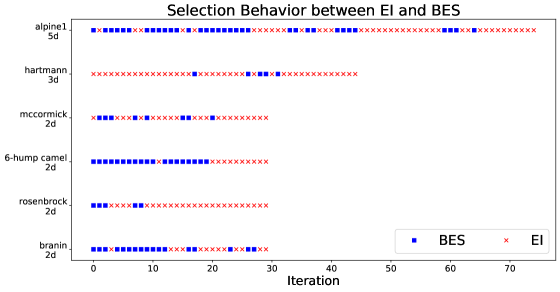
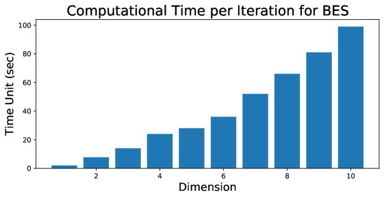
We report the time taken for computing bes per iteration in Fig. 10. We can see that the computational cost for bes increases with dimension. This is because the number of time required to evaluate the acquisition function will grow with dimension. Nevertheless, the overall cost for suggesting a point is still less than two minutes for d=10𝑑10d=10 while the black-box evaluation time is significantly higher, such as it takes a few hours to train a deep learning model.
Refer to caption
Figure 10: The computational cost for bes increases with dimension. Given an expensive black-box function f()𝑓f(\cdot) which can take hours for evaluation, our computational time is reasonable within less than two minutes for 101010 dimensions. The experiments are running on the Intel Core i7, 64GB Ram.

B.3 Decoupling Approach for gp Posterior Sampling

The central idea of decoupled sampling relies on the Matheron’s rule for Gaussian random variables (Journel and Huijbregts,, 1978; Chiles and Delfiner,, 2009; Doucet,, 2010) that uses variational Fourier features for an approximate prior and a deterministic data-dependent update term to efficiently draw samples. Let ϕ(𝐱i)=2lcos(θiT𝐱i+τi)italic-ϕsubscript𝐱𝑖2𝑙superscriptsubscript𝜃𝑖𝑇subscript𝐱𝑖subscript𝜏𝑖\phi(\mathbf{x}_{i})=\sqrt{\frac{2}{l}}\cos\left(\theta_{i}^{T}\mathbf{x}_{i}+\tau_{i}\right), where θisubscript𝜃𝑖\theta_{i} is sampled proportional to the kernel’s spectral density, τi𝕌(0,2π)similar-tosubscript𝜏𝑖𝕌02𝜋\tau_{i}\sim\mathbb{U}(0,2\pi) and l𝑙l is the random feature dimension. We draw samples f𝐗,𝐲,𝐱,ωmconditionalsubscript𝑓𝐗𝐲subscript𝐱subscript𝜔𝑚f_{*}\mid\mathbf{X},\mathbf{y},\mathbf{x}_{*},\omega_{m} from a gp posterior and evaluate them at any test input 𝐱𝒳subscript𝐱𝒳\mathbf{x}_{*}\in\mathcal{X} as

gm(𝐱)=i=1lwiϕi(𝐱)random+j=1Nvjk(𝐱,𝐱j)deterministic updatesubscript𝑔𝑚subscript𝐱superscriptsubscript𝑖1𝑙subscriptsubscript𝑤𝑖subscriptitalic-ϕ𝑖subscript𝐱randomsuperscriptsubscript𝑗1𝑁subscriptsubscript𝑣𝑗𝑘subscript𝐱subscript𝐱𝑗deterministic update\displaystyle\vspace{-10pt}g_{m}(\mathbf{x}_{*})=\sum_{i=1}^{l}\underbrace{w_{i}\phi_{i}(\mathbf{x}_{*})}_{\text{random}}+\sum_{j=1}^{N}\underbrace{v_{j}k(\mathbf{x}_{*},\mathbf{x}_{j})}_{\text{deterministic update}}\vspace{-10pt} (17)

where wiiid𝒩(0,1)subscript𝑤𝑖iidsimilar-to𝒩01w_{i}\overset{\textrm{iid}}{\sim}\mathcal{N}(0,1), 𝐰=[wi,,wl]Tl𝐰superscriptsubscript𝑤𝑖subscript𝑤𝑙𝑇superscript𝑙\mathbf{w}=[w_{i},...,w_{l}]^{T}\in\mathbb{R}^{l}, Φ=ϕ(𝐗)N×lΦitalic-ϕ𝐗superscript𝑁𝑙\Phi=\phi(\mathbf{X})\in\mathbb{R}^{N\times l} and v=(K+σf2𝐈)1(𝐲Φ𝐰)𝑣superscript𝐾superscriptsubscript𝜎𝑓2𝐈1𝐲Φ𝐰v=\big{(}K+\sigma_{f}^{2}\mathbf{I}\big{)}^{-1}\left(\mathbf{y}-\Phi\mathbf{w}\right). The sampling process above relies on the randomness of the Fourier features (Rahimi and Recht,, 2007) via ωmp(ω)similar-tosubscript𝜔𝑚𝑝𝜔\omega_{m}\sim p(\omega)

𝔼p(ω)[f𝐗,𝐲,ω]subscript𝔼𝑝𝜔delimited-[]conditionalsubscript𝑓𝐗𝐲𝜔\displaystyle\mathbb{E}_{p(\omega)}\left[f_{*}\mid\mathbf{X},\mathbf{y},\omega\right] 1Mωmp(ω)g(.𝐗,𝐲,ωm)\displaystyle\approx\frac{1}{M}\sum_{\omega_{m}\sim p(\omega)}g(.\mid\mathbf{X},\mathbf{y},\omega_{m}) (18)

where ωm={θm,τm}subscript𝜔𝑚subscript𝜃𝑚subscript𝜏𝑚\omega_{m}=\{\theta_{m},\tau_{m}\}.

B.4 Tightening the variances

To put things in context, the base distribution pbasesubscript𝑝basep_{\textrm{base}} for drawing gp posterior samples in Eq. (3) can be used as (i) standard gp (Wilson et al.,, 2020), (ii) weighting using gp (presented in Section 3.2) or (iii) weighting using srgp (Section 3.3), respectively. We denote these approaches as pgpsubscript𝑝gpp_{\lx@glossaries@gls@link{acronym}{GP}{\leavevmode\textsc{gp}}}, pw-gpsubscript𝑝w-gpp_{\textrm{w-}\lx@glossaries@gls@link{acronym}{GP}{\leavevmode\textsc{gp}}} and pw-srgpsubscript𝑝w-srgpp_{\textrm{w-}\lx@glossaries@gls@link{acronym}{SRGP}{\leavevmode\textsc{srgp}}}. We characterize the sample variance of the proposed approach and show that our strategy in weighting the gp posterior samples will tighten the variance of the gp samples considering in the 2d2𝑑2d space formed shown in Fig. 1 (left). We adapt the Popoviciu’s-inequality (Popoviciu,, 1935) to bound the variance in our two dimensional space considered in Fig. 1 (left).

Lemma 3.

Let l2𝑙superscript2l\in\mathbb{R}^{2} be a random variable restricted to [L1,U1]subscript𝐿1subscript𝑈1[L_{1},U_{1}] in the 1st dimension and [L2,U2]subscript𝐿2subscript𝑈2[L_{2},U_{2}] in the 2nd dimension, we bound the variance of l𝑙l as Var[l1](U1L1)24Vardelimited-[]subscript𝑙1superscriptsubscript𝑈1subscript𝐿124\textrm{Var}[l_{1}]\leq\frac{\left(U_{1}-L_{1}\right)^{2}}{4} and Var[l2](U2L2)24Vardelimited-[]subscript𝑙2superscriptsubscript𝑈2subscript𝐿224\textrm{Var}[l_{2}]\leq\frac{\left(U_{2}-L_{2}\right)^{2}}{4}.

Proof.

Let us denote [L1,L2]=inflsubscript𝐿1subscript𝐿2infimum𝑙[L_{1},L_{2}]=\inf\,l and [U1,U2]=suplsubscript𝑈1subscript𝑈2supremum𝑙[U_{1},U_{2}]=\sup\,l. We define a function hh by h(t)=𝔼[(lt)2]𝑡𝔼delimited-[]superscript𝑙𝑡2h(t)=\mathbb{E}\left[(l-t)^{2}\right] that h′′>0superscript′′0h^{\prime\prime}>0.

Computing the derivative hsuperscripth^{\prime}, and solving h(t)=2𝔼[l]+2t=0superscript𝑡2𝔼delimited-[]𝑙2𝑡0h^{\prime}(t)=-2\mathbb{E}[l]+2t=0, we find that g𝑔g achieves its minimum at t=𝔼[l]𝑡𝔼delimited-[]𝑙t=\mathbb{E}[l]. We then consider the value of the function hh at the specific point t=[U1+L12,U2+L22]𝑡subscript𝑈1subscript𝐿12subscript𝑈2subscript𝐿22t=\left[\frac{U_{1}+L_{1}}{2},\frac{U_{2}+L_{2}}{2}\right]. Next, we derive in the first dimension that

Var[l1]Vardelimited-[]subscript𝑙1\displaystyle\textrm{Var}[l_{1}] =h(𝔼[l1])h(U1+L12)absent𝔼delimited-[]subscript𝑙1subscript𝑈1subscript𝐿12\displaystyle=h\left(\mathbb{E}[l_{1}]\right)\leq h\left(\frac{U_{1}+L_{1}}{2}\right)
=𝔼[(l1U1+L12)2]by the definition ofh()absent𝔼delimited-[]superscriptsubscript𝑙1subscript𝑈1subscript𝐿122by the definition of\displaystyle=\mathbb{E}\left[\left(l_{1}-\frac{U_{1}+L_{1}}{2}\right)^{2}\right]\quad\quad\quad\quad\quad\quad\quad\quad\textrm{by\thinspace the\,definition\thinspace of}\thinspace h()
=14𝔼[((l1L1)+(l1U1))2]absent14𝔼delimited-[]superscriptsubscript𝑙1subscript𝐿1subscript𝑙1subscript𝑈12\displaystyle=\frac{1}{4}\mathbb{E}\left[\left((l_{1}-L_{1})+(l_{1}-U_{1})\right)^{2}\right]
14𝔼[(U1L1)2]=(U1L1)24.absent14𝔼delimited-[]superscriptsubscript𝑈1subscript𝐿12superscriptsubscript𝑈1subscript𝐿124\displaystyle\leq\frac{1}{4}\mathbb{E}\left[\left(U_{1}-L_{1}\right)^{2}\right]=\frac{\left(U_{1}-L_{1}\right)^{2}}{4}.

In the last inequality, we have ((l1L1)+(l1U1))2((l1L1)(l1U1))2=(U1L1)2superscriptsubscript𝑙1subscript𝐿1subscript𝑙1subscript𝑈12superscriptsubscript𝑙1subscript𝐿1subscript𝑙1subscript𝑈12superscriptsubscript𝑈1subscript𝐿12\bigl{(}(l_{1}-L_{1})+(l_{1}-U_{1})\bigr{)}^{2}\leq\bigl{(}(l_{1}-L_{1})-(l_{1}-U_{1})\bigr{)}^{2}=\bigl{(}U_{1}-L_{1}\bigr{)}^{2} due to l1L10subscript𝑙1subscript𝐿10l_{1}-L_{1}\geq 0 and l1U10subscript𝑙1subscript𝑈10l_{1}-U_{1}\leq 0. Similarly, we have the term in the second dimension bounded Var[l2](U2L2)24Vardelimited-[]subscript𝑙2superscriptsubscript𝑈2subscript𝐿224\textrm{Var}[l_{2}]\leq\frac{\left(U_{2}-L_{2}\right)^{2}}{4}. This concludes our proof. ∎

Lemma 4.

(Lemma 1 in the main paper) In the 2d space formed by [f+,f]superscript𝑓superscript𝑓\left[f^{+},f^{-}\right] and the gp posterior samples {gm+,gm}m=1Msuperscriptsubscriptsubscriptsuperscript𝑔𝑚subscriptsuperscript𝑔𝑚𝑚1𝑀\{g^{+}_{m},g^{-}_{m}\}_{m=1}^{M}, the sample variances by weighting our srgp and gp are smaller than the gp posterior sampling (Wilson et al.,, 2020) making no use of the bounds: Var[pw-gp]Var[pgp]Vardelimited-[]subscript𝑝w-gpVardelimited-[]subscript𝑝gp{\displaystyle\text{Var}\left[p_{\textrm{w-}\lx@glossaries@gls@link{acronym}{GP}{\leavevmode\textsc{gp}}}\right]}\leq{\displaystyle\text{Var}\left[p_{\lx@glossaries@gls@link{acronym}{GP}{\leavevmode\textsc{gp}}}\right]} and Var[pw-srgp]Var[pgp]Vardelimited-[]subscript𝑝w-srgpVardelimited-[]subscript𝑝gp{\displaystyle\text{Var}\left[p_{\textrm{w-}\lx@glossaries@gls@link{acronym}{SRGP}{\leavevmode\textsc{srgp}}}\right]}\leq{\displaystyle\text{Var}\left[p_{\lx@glossaries@gls@link{acronym}{GP}{\leavevmode\textsc{gp}}}\right]}.

Proof.

We first bound the sample variance in each dimension d={1,2}𝑑12d=\{1,2\} in Lemma 3 as Var[pgp(d)](Ugp(d)Lgp(d))24,Vardelimited-[]superscriptsubscript𝑝gp𝑑superscriptsuperscriptsubscript𝑈gp𝑑superscriptsubscript𝐿gp𝑑24\displaystyle{\displaystyle\text{Var}\left[p_{\textrm{\lx@glossaries@gls@link{acronym}{GP}{\leavevmode{gp}}}}^{(d)}\right]}\leq\frac{\left(U_{\textrm{\lx@glossaries@gls@link{acronym}{GP}{\leavevmode{gp}}}}^{(d)}-L_{\textrm{\lx@glossaries@gls@link{acronym}{GP}{\leavevmode{gp}}}}^{(d)}\right)^{2}}{4}, Var[pw-gp(d)]Vardelimited-[]superscriptsubscript𝑝w-gp𝑑\displaystyle{\displaystyle\text{Var}\left[p_{\textrm{w-\lx@glossaries@gls@link{acronym}{GP}{\leavevmode{gp}}}}^{(d)}\right]} (Uw-gp(d)Lw-gp(d))24absentsuperscriptsuperscriptsubscript𝑈w-gp𝑑superscriptsubscript𝐿w-gp𝑑24\displaystyle\leq\frac{\left(U_{\textrm{w-\lx@glossaries@gls@link{acronym}{GP}{\leavevmode{gp}}}}^{(d)}-L_{\textrm{w-\lx@glossaries@gls@link{acronym}{GP}{\leavevmode{gp}}}}^{(d)}\right)^{2}}{4}

where the base distribution can be used as (i) a standard gp, i.e., pgp=p(f()𝐗,𝐲)subscript𝑝gp𝑝conditional𝑓𝐗𝐲{\displaystyle p_{\textrm{\lx@glossaries@gls@link{acronym}{GP}{\leavevmode{gp}}}}}=p\bigl{(}f(\cdot)\mid\mathbf{X},\mathbf{y}\bigr{)} or (ii) a weighted gp with the bounds information pw-gp:=π(gm)=p(f()𝐗,𝐲,f+,f)assignsubscript𝑝w-gp𝜋subscript𝑔𝑚𝑝conditional𝑓𝐗𝐲superscript𝑓superscript𝑓{\displaystyle p_{\textrm{w-\lx@glossaries@gls@link{acronym}{GP}{\leavevmode{gp}}}}}:=\pi(g_{m})=p\bigl{(}f(\cdot)\mid\mathbf{X},\mathbf{y},f^{+},f^{-}\bigr{)}.

In our gp sampling and weighting setting, we have Uw-gp(d)<Ugp(d),d=1,2formulae-sequencesuperscriptsubscript𝑈w-gp𝑑superscriptsubscript𝑈gp𝑑for-all𝑑12U_{\textrm{w-\lx@glossaries@gls@link{acronym}{GP}{\leavevmode{gp}}}}^{(d)}<U_{\textrm{\lx@glossaries@gls@link{acronym}{GP}{\leavevmode{gp}}}}^{(d)},\forall d=1,2 and Lw-gp(d)>Lgp(d),dsuperscriptsubscript𝐿w-gp𝑑superscriptsubscript𝐿gp𝑑for-all𝑑L_{\textrm{w-\lx@glossaries@gls@link{acronym}{GP}{\leavevmode{gp}}}}^{(d)}>L_{\textrm{\lx@glossaries@gls@link{acronym}{GP}{\leavevmode{gp}}}}^{(d)},\forall d. This means Uw-gp(d)Lw-gp(d)Ugp(d)Lgp(d),dsuperscriptsubscript𝑈w-gp𝑑superscriptsubscript𝐿w-gp𝑑superscriptsubscript𝑈gp𝑑superscriptsubscript𝐿gp𝑑for-all𝑑U_{\textrm{w-\lx@glossaries@gls@link{acronym}{GP}{\leavevmode{gp}}}}^{(d)}-L_{\textrm{w-\lx@glossaries@gls@link{acronym}{GP}{\leavevmode{gp}}}}^{(d)}\leq U_{\textrm{\lx@glossaries@gls@link{acronym}{GP}{\leavevmode{gp}}}}^{(d)}-L_{\textrm{\lx@glossaries@gls@link{acronym}{GP}{\leavevmode{gp}}}}^{(d)},\forall d and thus Var[pw-gp]Var[pgp]Vardelimited-[]subscript𝑝w-gpVardelimited-[]subscript𝑝gp\text{Var}\left[p_{\textrm{w-\lx@glossaries@gls@link{acronym}{GP}{\leavevmode{gp}}}}\right]\leq\text{Var}\left[p_{\textrm{\lx@glossaries@gls@link{acronym}{GP}{\leavevmode{gp}}}}\right]. Using similar derivations, we get Var[pgp]Var[pw-srgp]Vardelimited-[]subscript𝑝gpVardelimited-[]subscript𝑝w-srgp{\displaystyle\text{Var}\left[p_{\lx@glossaries@gls@link{acronym}{GP}{\leavevmode\textsc{gp}}}\right]}\geq{\displaystyle\text{Var}\left[p_{\textrm{w-}\lx@glossaries@gls@link{acronym}{SRGP}{\leavevmode\textsc{srgp}}}\right]}, thus conclude the proof. ∎

This can also be seen in Fig. 1 that indeed π(gm)𝜋subscript𝑔𝑚\pi(g_{m}) is bounded by the density of pgpsubscript𝑝gpp_{\textrm{\lx@glossaries@gls@link{acronym}{GP}{\leavevmode{gp}}}}. Using srgp, we have flexibly transformed the surrogate toward the desirable area. Under such transformation, the pw-srgpsubscript𝑝w-srgpp_{\textrm{w-\lx@glossaries@gls@link{acronym}{SRGP}{\leavevmode{srgp}}}} has a tighter upper bound than pw-gpsubscript𝑝w-gpp_{\textrm{w-\lx@glossaries@gls@link{acronym}{GP}{\leavevmode{gp}}}}. We next show that the sample variance of the base distribution using weighting srgp is smaller than using weighting gp, Var[pw-srgp]Var[pw-gp]Vardelimited-[]subscript𝑝w-srgpVardelimited-[]subscript𝑝w-gp{\displaystyle\text{Var}\left[p_{\textrm{w-\lx@glossaries@gls@link{acronym}{SRGP}{\leavevmode{srgp}}}}\right]\leq\text{Var}\left[p_{\textrm{w-\lx@glossaries@gls@link{acronym}{GP}{\leavevmode{gp}}}}\right]}. Thus, the srgp is more sample-efficient than gp in generating accepted samples. This variance property can be intuitively seen from Fig. 1 (left) in the main paper. In addition, we have numerically demonstrated this comparison in Table 1.

Lemma 5.

(Lemma 2 in the main paper) In the 2d space formed by [f+,f]superscript𝑓superscript𝑓\left[f^{+},f^{-}\right] and the gp posterior samples {gm+,gm}m=1Msuperscriptsubscriptsubscriptsuperscript𝑔𝑚subscriptsuperscript𝑔𝑚𝑚1𝑀\{g^{+}_{m},g^{-}_{m}\}_{m=1}^{M}, the sample variance of weighting srgp is smaller than weighting gp: Var[pw-srgp]Var[pw-gp]Vardelimited-[]subscript𝑝w-srgpVardelimited-[]subscript𝑝w-gp\text{Var}\left[p_{\textrm{w-\lx@glossaries@gls@link{acronym}{SRGP}{\leavevmode{srgp}}}}\right]\leq{\displaystyle\text{Var}\left[p_{\textrm{w-\lx@glossaries@gls@link{acronym}{GP}{\leavevmode{gp}}}}\right]}.

Proof.

To prove Var[pw-srgp]Var[pw-gp]Vardelimited-[]subscript𝑝w-srgpVardelimited-[]subscript𝑝w-gp\text{Var}\left[p_{\textrm{w-\lx@glossaries@gls@link{acronym}{SRGP}{\leavevmode{srgp}}}}\right]\leq{\displaystyle\text{Var}\left[p_{\textrm{w-\lx@glossaries@gls@link{acronym}{GP}{\leavevmode{gp}}}}\right]}, it is equivalent to show that the inequality is true in all dimensions of the distributions considered. Let us denote the first dimension (1)1(1) is formed by f+maxgm()superscript𝑓subscript𝑔𝑚f^{+}-\max g_{m}(\cdot) and the second dimension (2)2(2) is by fmingm()superscript𝑓subscript𝑔𝑚f^{-}-\min g_{m}(\cdot), see Fig. 1. In the first dimension, we have the upper bound Uw-srgp(1)=f++2η+Uw-gp(1)superscriptsubscript𝑈w-srgp1superscript𝑓2subscript𝜂superscriptsubscript𝑈w-gp1U_{\textrm{w-\lx@glossaries@gls@link{acronym}{SRGP}{\leavevmode{srgp}}}}^{(1)}=f^{+}+2\eta_{+}\leq U_{\textrm{w-\lx@glossaries@gls@link{acronym}{GP}{\leavevmode{gp}}}}^{(1)}, the equality happens when η+subscript𝜂\eta_{+}\rightarrow\infty and the lower bound Lw-gp(1)=Lw-srgp(1)superscriptsubscript𝐿w-gp1superscriptsubscript𝐿w-srgp1L_{\textrm{w-\lx@glossaries@gls@link{acronym}{GP}{\leavevmode{gp}}}}^{(1)}=L_{\textrm{w-\lx@glossaries@gls@link{acronym}{SRGP}{\leavevmode{srgp}}}}^{(1)}. In the second dimension, we have both the upper and lower bounds unchanged Uw-gp(2)=Uw-srgp(2)superscriptsubscript𝑈w-gp2superscriptsubscript𝑈w-srgp2U_{\textrm{w-\lx@glossaries@gls@link{acronym}{GP}{\leavevmode{gp}}}}^{(2)}=U_{\textrm{w-\lx@glossaries@gls@link{acronym}{SRGP}{\leavevmode{srgp}}}}^{(2)} and Lw-gp(2)=Lw-srgp(2)superscriptsubscript𝐿w-gp2superscriptsubscript𝐿w-srgp2L_{\textrm{w-\lx@glossaries@gls@link{acronym}{GP}{\leavevmode{gp}}}}^{(2)}=L_{\textrm{w-\lx@glossaries@gls@link{acronym}{SRGP}{\leavevmode{srgp}}}}^{(2)}.

Using Lemma 3, we conclude that Var[pw-srgp(1)]Var[pw-gp(1)]Vardelimited-[]superscriptsubscript𝑝w-srgp1Vardelimited-[]superscriptsubscript𝑝w-gp1\text{Var}\left[p_{\textrm{w-\lx@glossaries@gls@link{acronym}{SRGP}{\leavevmode{srgp}}}}^{(1)}\right]\leq{\displaystyle\text{Var}\left[p_{\textrm{w-\lx@glossaries@gls@link{acronym}{GP}{\leavevmode{gp}}}}^{(1)}\right]} and Var[pw-srgp(2)]Var[pw-gp(2)]Vardelimited-[]superscriptsubscript𝑝w-srgp2Vardelimited-[]superscriptsubscript𝑝w-gp2\text{Var}\left[p_{\textrm{w-\lx@glossaries@gls@link{acronym}{SRGP}{\leavevmode{srgp}}}}^{(2)}\right]\leq{\displaystyle\text{Var}\left[p_{\textrm{w-\lx@glossaries@gls@link{acronym}{GP}{\leavevmode{gp}}}}^{(2)}\right]}. In words, the base distribution by srgp (Section 3.3) pw-srgpsubscript𝑝w-srgpp_{\textrm{w-\lx@glossaries@gls@link{acronym}{SRGP}{\leavevmode{srgp}}}} has a tighter sample variance than pw-gpsubscript𝑝w-gpp_{\textrm{w-\lx@glossaries@gls@link{acronym}{GP}{\leavevmode{gp}}}} (Wilson et al.,, 2020). ∎

B.5 Derivations of the posterior approximation in Eq. (6) and Eq. (7)

We follow existing works, such as Gunter et al., (2014); Ru et al., (2018); Nguyen and Osborne, (2020) to approximate p(f(𝐱)𝐗,𝐲,η+,f+)𝑝conditional𝑓subscript𝐱𝐗𝐲subscript𝜂superscript𝑓p\bigl{(}f(\mathbf{x}_{*})\mid\mathbf{X},\mathbf{y},\eta_{+},f^{+}\bigr{)} with a Gaussian distribution by using a Taylor approximation.

Given f(𝐱)=f++2η+12h2(𝐱)𝑓𝐱superscript𝑓2subscript𝜂12superscript2𝐱f(\mathbf{x})=f^{+}+2\eta_{+}-\frac{1}{2}h^{2}(\mathbf{x}) from Eq. (5), we perform a local linearisation of the parabolic transformation q(h(𝐱))=f++2η+12h2(𝐱)𝑞𝐱superscript𝑓2subscript𝜂12superscript2𝐱q\bigl{(}h(\mathbf{x})\bigr{)}=f^{+}+2\eta_{+}-\frac{1}{2}h^{2}(\mathbf{x}) around h0subscript0h_{0} to obtain f(h)q(h0)+q(h0)(hh0)+𝑓𝑞subscript0superscript𝑞subscript0subscript0f(h)\approx q(h_{0})+q^{\prime}(h_{0})(h-h_{0})+... where the gradient q(h0)=hsuperscript𝑞subscript0q^{\prime}(h_{0})=-h. Then we set h0=mhsubscript0subscript𝑚h_{0}=m_{h} where mhsubscript𝑚m_{h} is defined in Eq. (5) to obtain an expression for f𝑓f which is linear in hh

f(𝐱)𝑓𝐱\displaystyle f(\mathbf{x}) q(h0(𝐱))+q(h0(𝐱))(h(𝐱)h0(𝐱))absent𝑞subscript0𝐱superscript𝑞subscript0𝐱𝐱subscript0𝐱\displaystyle\approx q\bigl{(}h_{0}(\mathbf{x})\bigr{)}+q^{\prime}\bigl{(}h_{0}(\mathbf{x})\bigr{)}\bigl{(}h(\mathbf{x})-h_{0}(\mathbf{x})\bigr{)} (19)
=[f++2η+12mh2(𝐱)]mh(𝐱)[h(𝐱)mh(𝐱)]absentdelimited-[]superscript𝑓2subscript𝜂12superscriptsubscript𝑚2𝐱subscript𝑚𝐱delimited-[]𝐱subscript𝑚𝐱\displaystyle=\bigl{[}f^{+}+2\eta_{+}-\frac{1}{2}m_{h}^{2}(\mathbf{x})\bigr{]}-m_{h}(\mathbf{x})\bigl{[}h(\mathbf{x})-m_{h}(\mathbf{x})\bigr{]} (20)
=f++2η++12mh2(𝐱)mh(𝐱)h(𝐱)absentsuperscript𝑓2subscript𝜂12superscriptsubscript𝑚2𝐱subscript𝑚𝐱𝐱\displaystyle=f^{+}+2\eta_{+}+\frac{1}{2}m_{h}^{2}(\mathbf{x})-m_{h}(\mathbf{x})h(\mathbf{x}) (21)

We make use an important property that the affine transformation of a Gaussian process remains Gaussian. We state the property as follows: let y=A𝐱+t𝑦𝐴𝐱𝑡y=A\mathbf{x}+t , 𝐱𝒩(μ𝐱,σ𝐱)similar-to𝐱𝒩subscript𝜇𝐱subscript𝜎𝐱\mathbf{x}\sim\mathcal{N}(\mu_{\mathbf{x}},\sigma_{\mathbf{x}}), then y=𝒩(Aμ𝐱+t,Aσ𝐱A)𝑦𝒩𝐴subscript𝜇𝐱𝑡𝐴subscript𝜎𝐱𝐴y=\mathcal{N}(A\mu_{\mathbf{x}}+t,A\sigma_{\mathbf{x}}A).

Let apply this property into our setting. Given h𝒩(μh,σh2)similar-to𝒩subscript𝜇subscriptsuperscript𝜎2h\sim\mathcal{N}(\mu_{h},\sigma^{2}_{h}) and f𝒩(μf,σf)similar-to𝑓𝒩subscript𝜇𝑓subscript𝜎𝑓f\sim\mathcal{N}(\mu_{f},\sigma_{f}), we obtain

μfsubscript𝜇𝑓\displaystyle\mu_{f} =f++2η++12μh2μh2=f++2η+12μh2absentsuperscript𝑓2subscript𝜂12superscriptsubscript𝜇2superscriptsubscript𝜇2superscript𝑓2subscript𝜂12superscriptsubscript𝜇2\displaystyle=f^{+}+2\eta_{+}+\frac{1}{2}\mu_{h}^{2}-\mu_{h}^{2}=f^{+}+2\eta_{+}-\frac{1}{2}\mu_{h}^{2} (22)
σf2subscriptsuperscript𝜎2𝑓\displaystyle\sigma^{2}_{f} =μhσh2μhabsentsubscript𝜇subscriptsuperscript𝜎2subscript𝜇\displaystyle=\mu_{h}\sigma^{2}_{h}\mu_{h} (23)

as shown in Eq. (6) and Eq. (7) in the main paper.

Appendix C Ablation Studies

C.1 Ablation studies with different numbers of gp samples M𝑀M

We study the sensitivity with varying the number of gp samples M[20,50,200,300,500]𝑀2050200300500M\in[20,50,200,300,500] in Fig. 11. We show that if the number of M𝑀M is set too small, such as M50𝑀50M\leq 50. The performance can be negatively affected. On the other hand, if we set M𝑀M large enough to be [200,500]200500[200,500], they tend to perform similarly well. This is the recommended range for M𝑀M in our paper. We also note that increasing M𝑀M will require more computation. However, such computation can be well handled by using parallel infrastructure since drawing gp samples are independent of each other.
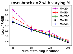
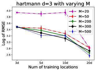
Refer to caption
Refer to caption
Refer to caption
Figure 11: gp posterior sampling with different number of gp samples M𝑀M. Our approach using M[200,500]𝑀200500M\in[200,500] will result in the best performance while M=20𝑀20M=20 is the worst.
Refer to caption
Figure 12: When none of the gp sample is accepted (falling into the two standard deviation of π(gm)𝜋subscript𝑔𝑚\pi(g_{m})), we propose to use the ei instead of bes. This illustration indicates the switching behavior between ei vs bes.

C.2 Switching between ei vs bes

We have discussed in Section 6 that there will be some iterations when we don’t have any accepted sample for bes. There are several reasons, such as the observations are biased to reconstruct the black-box function, the estimated gp hyperparameters are not correct. When the number of accepted samples is zero, we will perform Expected improvement (Jones et al.,, 1998) instead of bes. Our choice is motivated by the strong and robust performance of ei. We note that an alternative solution is to keep sampling the gp until we get at least one accepted sample.

We illustrate this behavior in Fig. 12. We use the number of gp samples M=200𝑀200M=200, η+2=0.03dsubscriptsuperscript𝜂20.03𝑑\eta^{2}_{+}=0.03d and η2=0.6dsubscriptsuperscript𝜂20.6𝑑\eta^{2}_{-}=0.6d where d𝑑d is the input dimension. We use a blue square to indicate if bes is used for this iteration and red cross if ei is taken.
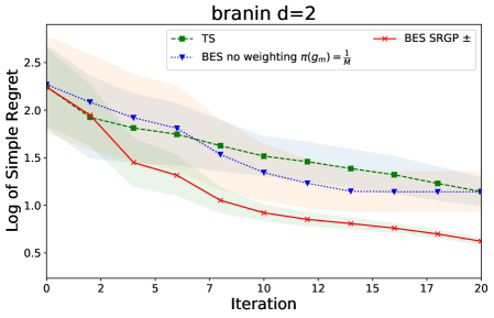
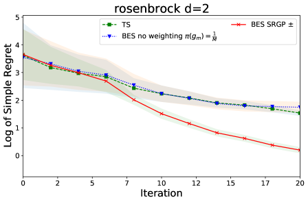
Refer to caption
Refer to caption
Refer to caption
Refer to caption
Figure 13: Ablation studies of bes without weighting or π(gm)=1M𝜋subscript𝑔𝑚1𝑀\pi(g_{m})=\frac{1}{M}. The weighting step significantly boosts the performance of bes to achieve significantly better than bes without weighting (blue curve). Simple regret is defined as the gap between the optimum value and the best found value, i.e., |max𝐱𝒳f(𝐱)max𝐱iDtf(𝐱i)|subscriptfor-all𝐱𝒳𝑓𝐱subscriptfor-allsubscript𝐱𝑖subscript𝐷𝑡𝑓subscript𝐱𝑖|\max_{\forall\mathbf{x}\in\mathcal{X}}f(\mathbf{x})-\max_{\forall\mathbf{x}_{i}\in D_{t}}f(\mathbf{x}_{i})|.

C.3 BES without weighting

We provide another set of experiments to compare the performance with a variant version of bes without weighting and Thompson sampling (or bes with M=1𝑀1M=1). The bes setting without weighting is when we ignore the f+superscript𝑓f^{+}, fsuperscript𝑓f^{-} and set the weighting probability π(gm)=1M𝜋subscript𝑔𝑚1𝑀\pi(g_{m})=\frac{1}{M} uniformly.

Fig. 13 shows that bes without weighting (blue curve) will perform poorly. Particularly, this version will accept all gp posterior samples and gain information about all of them, including the ‘bad’ samples. Thompson sampling (ts) is a special version of bes in which we only draw a single gp posterior sample g()𝑔g(\cdot). Then, we select a next point to evaluate as the mode of this sample, i.e., 𝐱t=argmax𝐱𝒳g(𝐱)subscript𝐱𝑡subscript𝐱𝒳𝑔𝐱\mathbf{x}_{t}=\arg\max_{\mathbf{x}\in\mathcal{X}}g(\mathbf{x}). Because drawing a single gp sample will have very high variance especially in high-dimension, ts will generally perform inferior in a sequential bo setting, as discussed in Hernández-Lobato et al., (2014); Nguyen et al., (2019).

Exploiting the knowledge about both f+,fsuperscript𝑓superscript𝑓f^{+},f^{-} will result in better performance than exploiting a single value of f+superscript𝑓f^{+}. Especially, our bes version using square-root transformation gp will achieve the best performance. This is because it can take into account the knowledge of f+superscript𝑓f^{+} to tailor the gp sample toward the desirable shape. This will lead to better theoretical property as presented in Lemma 1 and Lemma 2.

The result in this experiment again highlights our choice of bes in Section 4 that gains information only about good gp posterior samples.

Refer to caption
Refer to caption
Refer to caption
Refer to caption
Refer to caption
Figure 14: We study the sensitivity of the model by misspecifying the f+superscript𝑓f^{+} and fsuperscript𝑓f^{-} with different levels η2:=η+2=η2[0,1,3,5]assignsuperscript𝜂2subscriptsuperscript𝜂2subscriptsuperscript𝜂20135\eta^{2}:=\eta^{2}_{+}=\eta^{2}_{-}\in[0,1,3,5]. Increasing the misspecified levels will degrade the performance. It is important to note that our w-gp with misspecification still performs better than the vanilla gp sampling (Wilson et al.,, 2020) which does not use the bounds, especially when the number of training locations is small, 3d3𝑑3d or 5d5𝑑5d. Asymptotically, when η𝜂\eta\rightarrow\infty, our w-gp will accept all samples and become the case of Wilson et al., (2020).

C.4 Sensitivity analysis of misspecifying f+superscript𝑓f^{+} and fsuperscript𝑓f^{-} for gp posterior sampling

We study the sensitivity to the gp posterior sampling performance by misspecifying the upper and lower bounds. In the benchmark function considered, we know the true maxf(𝐱)𝑓𝐱\max f(\mathbf{x}) and minf(𝐱)𝑓𝐱\min f(\mathbf{x}) in advance. We make use of these optimum values and vary the misspecified levels η+2=η2[0,1,3,5]subscriptsuperscript𝜂2subscriptsuperscript𝜂20135\eta^{2}_{+}=\eta^{2}_{-}\in\left[0,1,3,5\right] for which f+=maxf(𝐱)+𝒩(0,η+2)superscript𝑓𝑓𝐱𝒩0subscriptsuperscript𝜂2f^{+}=\max f(\mathbf{x})+\mathcal{N}(0,\eta^{2}_{+}) and f=minf(𝐱)+𝒩(0,η2)superscript𝑓𝑓𝐱𝒩0subscriptsuperscript𝜂2f^{-}=\min f(\mathbf{x})+\mathcal{N}(0,\eta^{2}_{-}). This level is considered in a standardized output space y𝒩(0,1)similar-to𝑦𝒩01y\sim\mathcal{N}(0,1). We present the result in Fig. 14. It is expected that increasing the misspecified levels will lead to degrading the performance. However, our model still performs better than the vanilla gp sampling (Wilson et al.,, 2020) in most cases. Especially when we have limited observations of less than 5d5𝑑5d training locations, our model outperforms gp sampling when η23superscript𝜂23\eta^{2}\leq 3.

Relaxing this misspecify level η𝜂\eta\rightarrow\infty will let the performance of w-gp at least reduce to the case of Wilson et al., (2020) while the performance of w-srgp will be more sensitive as the transformation depends on η+subscript𝜂\eta_{+}.

Appendix D Experimental evaluation

D.1 Experimental setting

The benchmarks function and their ranges are available online.444https://www.sfu.ca/~ssurjano/optimization.html We summarize the hyperparameters and their min-max ranges used in the machine learning tuning experiments in Table 2.

  • Support vector regression (Smola and Vapnik,, 1997) on Abalone dataset. The Abalone dataset is available publicly.555https://archive.ics.uci.edu/ml/datasets/abalone We specify the upper bound as f+=1.92superscript𝑓1.92f^{+}=-1.92 and do not set the lower bound.

  • xgboost classification (Chen and Guestrin,, 2016): we use Pima Indians Diabetes database.666https://www.kaggle.com/uciml/pima-indians-diabetes-database We set the bounds f+=0.75superscript𝑓0.75f^{+}=0.75, f=0.65superscript𝑓0.65f^{-}=0.65 for the result presented in Fig. 4. Then, we vary the upper bound f+[0.7,0.73,0.75,0.77,0.8,0.9]superscript𝑓0.70.730.750.770.80.9f^{+}\in[0.7,0.73,0.75,0.77,0.8,0.9] to study the sensitivity with different choices of f+superscript𝑓f^{+} presented in Fig. 7.

  • cnn classification (LeCun and Bengio,, 1995) on a subset (10%) of cifar10. We use the bounds of f+=61.5superscript𝑓61.5f^{+}=61.5 and f=0superscript𝑓0f^{-}=0.

Table 2: The ranges for each hyperparameter used for tuning machine learning algorithms.
xgboost
Variables Min Max
min_child_weight 111 202020
colsample_bytree 0.10.10.1 111
max_depth 555 151515
subsample 0.50.50.5 111
gamma 00 101010
alpha 00 101010
cnn
Variables Min Max
batch size 161616 100100100
learning rate 1e61superscript𝑒61e^{-6} 1e21superscript𝑒21e^{-2}
max iteration 555 505050
Support vector regression
Variables Min Max
C𝐶C 0.10.10.1 100010001000
epsilon 1e61superscript𝑒61e^{-6} 111
gamma 1e61superscript𝑒61e^{-6} 555

D.2 Additional experiments

We present additional experiments for gp posterior sampling in Fig. 15 and Bayesian optimization in Fig. 16. The additional results are consistent with the results presented in the main paper. bes ±plus-or-minus\pm (exploiting both f+superscript𝑓f^{+} and fsuperscript𝑓f^{-}) achieves the best performance.
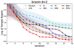
Refer to caption
Refer to caption
Refer to caption
Refer to caption
Refer to caption
Refer to caption
Refer to caption
Figure 15: We measure the root mean squared error (rmse) loss from M=200𝑀200M=200 gp samples g()𝑔g(\cdot) against the true function f()𝑓f(\cdot) with different number of training points [3d,5d,10d,20d]3𝑑5𝑑10𝑑20𝑑[3d,5d,10d,20d] where d𝑑d is the number of input dimensions. The f+superscript𝑓f^{+} and fsuperscript𝑓f^{-} are known from the black-box function. The overall trends indicate that (i) the loss is smaller with increasing number of training points and (ii) exploiting the external knowledge about f+superscript𝑓f^{+} and fsuperscript𝑓f^{-} will lead to better estimation than exploiting f+superscript𝑓f^{+} alone. When we get sufficient observations, e.g., the number of training locations is 20d20𝑑20d, the performance of w-gp f+,fsuperscript𝑓superscript𝑓f^{+},f^{-} resembles w-srgp f+,fsuperscript𝑓superscript𝑓f^{+},f^{-}. The error bar is estimated over 303030 independent runs.
Refer to caption
Refer to caption
Refer to caption
Refer to caption
Refer to caption
Refer to caption
Figure 16: We present additional results for Bayesian optimization using benchmark functions. Our bes ±plus-or-minus\pm (using both f+,fsuperscript𝑓superscript𝑓f^{+},f^{-}) achieves better performance than bes ++ (using f+superscript𝑓f^{+} alone) and erm (using f+superscript𝑓f^{+} alone) (Nguyen and Osborne,, 2020). Simple regret is defined as |max𝐱𝒳f(𝐱)max𝐱iDtf(𝐱i)|subscriptfor-all𝐱𝒳𝑓𝐱subscriptfor-allsubscript𝐱𝑖subscript𝐷𝑡𝑓subscript𝐱𝑖|\max_{\forall\mathbf{x}\in\mathcal{X}}f(\mathbf{x})-\max_{\forall\mathbf{x}_{i}\in D_{t}}f(\mathbf{x}_{i})|.