Entropy-Stable Schemes in the Low-Mach-Number Regime: Flux-Preconditioning, Entropy Breakdowns, and Entropy Transfers

Abstract

Entropy-Stable (ES) schemes, specifically those built from [Tadmor Math. Comput. 49 (1987) 91], have been gaining interest over the past decade, especially in the context of under-resolved simulations of compressible turbulent flows using high-order methods. These schemes are attractive because they can provide stability in a global and nonlinear sense (consistency with thermodynamics). However, fully realizing the potential of ES schemes requires a better grasp of their local behavior. Entropy-stability itself does not imply good local behavior [Gouasmi et al. J. Sci. Comp. 78 (2019) 971, Gouasmi et al. Comput. Methd. Appl. M. 363 (2020) 112912]. In this spirit, we studied ES schemes in problems where global stability is not the core issue. In the present work, we consider the accuracy degradation issues typically encountered by upwind-type schemes in the low-Mach-number regime [Turkel Annu. Rev. Fluid Mech. 31 (1999) 285] and their treatment using Flux-Preconditioning [Turkel J. Comput. Phys. 72 (1987) 277, Miczek et al. A & A 576 (2015) A50]. ES schemes suffer from the same issues and Flux-Preconditioning can improve their behavior without interfering with entropy-stability. This is first demonstrated analytically: using similarity and congruence transforms we were able to establish conditions for a preconditioned flux to be ES, and introduce the ES variants of the Miczek’s and Turkel’s preconditioned fluxes. This is then demonstrated numerically through first-order simulations of two simple test problems representative of the incompressible and acoustic limits, the Gresho Vortex and a right-moving acoustic wave. The results are overall consistent with previous studies. For instance, we observe that Turkel’s preconditioner improves accuracy in the incompressible limit with the downside of overly damping acoustic waves [Bruel et al. J. Comput. Phys. 378 (2019) 723]. For Miczek’s matrix however, we came across unexpected spurious transients in both problems (a small left-moving acoustic wave in the latter), motivating further analysis. We revisited the pressure fluctuation argument of [Guillard & Viozat Comput. Fluids 28 (1999) 63] in terms of entropy, showing how the standard ES dissipation operator [Ismail & Roe J. Comput. Phys. 228 (2009) 5410] can introduce inconsistent discrete entropy fluctuations in space. These analytical results are achieved by introducing mode-by-mode decompositions of the dissipation operator, similar to [Roe & Pike Computing Methods in Applied Science and Engineering (1984) 499, Tadmor Acta Numer. 12 (2003) 482], leading to what we call discrete Entropy Production Breakdowns (EPBs) in space. These EPBs outline the contributions of convective and acoustic modes to the discrete entropy production, both locally and globally. Ultimately, these EPBs enable us to single-out in the ES Miczek flux a skew-symmetric matrix component which we believe causes entropy transfers between acoustic waves. Removing this contribution eliminates the spurious transients without interfering with entropy-stability. This conjecture is explored numerically and analytically.

1 Introduction

Entropy-Stable (ES) schemes have been gaining interest over the past decade, especially in the context of under-resolved simulations of compressible turbulent flows using high-order methods HO ; ES_Diosady ; ES_Pazner ; ES_Fernandez . ES schemes are attractive because they can provide stability in both an integral and a nonlinear sense. These schemes are based on the mathematical structure that some systems of Partial Differential Equations (PDEs), such as the compressible Euler equations, possess. These systems, which we write:

$$\frac{\partial\mathbf{u}}{\partial t}+\sum_{j=1}^{d}\frac{\partial\mathbf{f}_{j}}{\partial x_{j}}=0,$$ (1)

where $\mathbf{u}$ and $(\mathbf{f}_{j})_{1\leq d\leq 3}$ are the state and flux vectors, respectively, and $d$ denotes the number of spatial dimensions, are known to admit a convex extension ES_Friedrichs ; ES_Harten in the sense that they imply an additional conservation equation for a convex scalar function $U$ (commonly referred to as a mathematical entropy):

$$\frac{\partial U}{\partial t}+\sum_{j=1}^{d}\frac{\partial F_{j}}{\partial x_{j}}=0.$$ (2)

The pair $(U,\ F_{j})=(U(\mathbf{u}),F_{j}(\mathbf{u}))\in\mathbb{R}\times\mathbb{R}^{d}$ must satisfy compatibility relations for the baseline system (1) to imply equation (2). Mathematical entropies have proven to be a key tool in the analysis and discretization of systems of conservation laws ES_Tadmor_2003 . The existence of a mathematical entropy implies that the PDE system can be symmetrized, which implies its hyperbolicity, and some local existence results. Most notably, a regularization argument by Lax leads to the requirement that admissible weak solutions must satisfy, in the sense of distributions, the entropy inequality:

$$\frac{\partial U}{\partial t}+\sum_{j=1}^{d}\frac{\partial F_{j}}{\partial x_{j}}<0.$$ (3)

Integrating this inequality over a spatial domain $\Omega$ of trace $\Gamma$, one gets:

$$\frac{d}{dt}\bigg{(}\int_{\Omega}UdV\bigg{)}\ +\ \oint_{\Gamma}F_{n}dS\ \leq\ 0,$$ (4)

where $F_{n}$ denotes the entropy flux projected onto the normal to the local surface element $dS$ of $\Gamma$. If the boundary term is positive or zero (periodic flow), inequality (3) becomes a nonlinear integral bound on the solution. This entropy stability property has been actively sought in the development of robust high-order schemes. According to the CFD 2030 Vision Study HO : ”Longer term, high-risk research should focus on the development of truly enabling technologies such as monotone or entropy stable schemes”. Efforts are being spent on the development of code infrastructures that can make the most out of ES schemes: the eddy solver eddy0 ; eddy1 ; ES_Diosady under development at NASA Ames Research Center for the simulation of turbulent separated flows and more recently for multi-physics applications is one of several examples.
A variety of ES scheme formulations can be found in the literature. Perhaps the most well-known ones are first-order finite-volume Godunov-type schemes ES_Harten , which consist in using solutions of the Riemann problem to compute flux contributions at interfaces. The Godunov scheme, which uses the exact solution to the Riemann problem, is ES as long as the exact Riemann solution exists and satisfies (3). Harten et al. ES_Harten showed that Godunov-type schemes using approximate Riemann solutions (the HLL scheme for instance) are ES if the approximate Riemann solution satisfies (3). The Lax-Friedrichs scheme is another well-known ES scheme (an elegant algebraic proof was given by Lax ES_Lax ). These first-order ES schemes can be used as building blocks for high-order fully-discrete ES schemes by leveraging the convexity of $U$ through convex combinations (see Gottlieb et al. Gottlieb and Guermond et al. for Guermond_0 ; Guermond_1 ). Some finite-element high-order ES discretizations stem from the seminal work of Hughes et al. ES_Hughes who showed that a continuous-Galerkin discretization of systems such as (1) of arbitrary order can be made ES a priori if the local polynomial representation of the finite-element solution is assigned to the so-called entropy variables instead of the conserved variables. Barth extended these ideas to the discontinuous-Galerkin method ES_Barth .
In a seminal paper ES_Tadmor_1987 , Tadmor introduced finite-volume/finite-difference schemes that achieve entropy-stability in a way that sets them apart from all of the aforementioned ES schemes. Rather than seeking to meet the entropy inequality directly (3), Tadmor first developed Entropy Conservative (EC) schemes, namely schemes that are consistent with the conservation equation (2). These require EC numerical flux functions, characterized by a scalar entropy conservation jump condition. Entropy-Stability is then achieved by adding an appropriate dissipation term to the EC flux (the resulting flux is termed ES). From there, a number a developments followed, mostly focused on high-order discretizations ES_Fisher ; ES_Fried ; ES_Fjordholm ; ES_Pazner ; ES_Fernandez . The present work is exclusively concerned with ES formulations building from Tadmor’s ground ideas.
This focus follows from the authors’ stance Gouasmi_Thesis that ES schemes could be developed into a solid numerical foundation in the simulation of compressible turbulent flows. A key undertaking to fully realize this vision is to better grasp the local behavior of ES schemes. In this endeavor, the authors have been studying ES schemes in problems where global stability is not the core issue Gouasmi_0 ; Gouasmi_2 . A rationale around this stance and approach is given in Gouasmi’s PhD thesis Gouasmi_Thesis .
Numerical schemes designed for compressible flows are known to perform poorly in the low-Mach-number regime Volpe ; Turkel0 ; Merkle ; Turkel2005 , more specifically in the incompressible limit, despite the fact that the incompressible Euler equations are a particular occurrence of the more general compressible Euler equations Schochet ; Majda . As there are many flow configurations of engineering interest that exhibit both compressible and incompressible flow phenomena (transonic flow, subsonic combustion, nozzle flows and shock-induced shear instabilities among others), significant research effort has been dedicated to adapting compressible flow codes to handle incompressible flows better. Steady state calculations, which are typically carried out by evolving the unsteady system until a stationary solution is found, require a number of iterations which dramatically increases as the Mach number decreases. Preconditioning methods Turkel0 ; Turkel1 ; Turkel1994 ; Turkel2005 ; Guillard1 ; Guillard2 ; Weiss ; Lee ; Merkle have been developed to address this stiffness issue. The idea is to modify the temporal scales of the unsteady system that is iterated by pre-multiplying the time derivative by a well-chosen preconditioning matrix $P$, in order to accelerate convergence. In addition to stiffness, the accuracy of the solution is also known to degrade. The root cause of this issue lies in the artificial viscosity introduced by upwind fluxes. Turkel Turkel0 ; Turkel1 ; Turkel1994 ; Turkel2005 and Guillard & Viozat Guillard1 showed in different ways that the dissipation term $|A|[\mathbf{u}]=R|\Lambda|R^{-1}[\mathbf{u}]$ of upwind fluxes contains terms which prevent the discrete equations solving the compressible system to converge to a set of discrete equations solving the incompressible system. The accuracy degradation problems can be alleviated with Flux-Preconditioning, which consists in modifying the upwind dissipation using matrix operations ($P^{-1}|PA|[\mathbf{u}]$ - this operation arises naturally when introducing upwinding in the preconditioned system). For unsteady flows, similar stiffness (stringent CFL condition warrants implicit temporal schemes, whose solution using Newton/GMRES approaches requires efficient preconditioning) and accuracy (excessive damping of vortical structures Miczek_T ; Miczek ; Barsukow ; Thornber1 ; Thornber2 due to upwinding) issues arise and can be dealt with similarly.
The present work Gouasmi_USNCCM considers the accuracy degradation problem in the context of ES schemes. Our first goal was to establish whether Flux-Preconditioning and Entropy-Stability are compatible. We considered two preconditioning matrices: one of the earliest ones by Turkel Turkel0 ; Turkel1 ; Turkel1994 and a more recent one by Miczek Miczek ; Miczek_T . ES schemes are subject to the same accuracy issues as standard Roe-type schemes because the dissipation terms they use also involves some form of upwinding ($R|\Lambda|R^{T}[\mathbf{v}]$). We posed the compatibility problem as a linear algebra problem involving $P$. Using similarity and congruence transforms, we established a sufficient condition for compatibility using Barth’s eigenscaling theorem. This condition is met by Turkel’s preconditioner but does not allow a statement to be made regarding Miczek’s preconditioner, whose compatibility is eventually proved using different arguments. From there, we compared four different numerical fluxes in space with Backward Euler in time on two simple periodic flow problems: the Gresho Vortex (incompressible limit) in two dimensions and a right-moving acoustic wave in one dimension (acoustic limit). They use the same EC flux ES_Chandra , but differ in their dissipation components. The first flux uses the standard ES dissipation operator Roe (ES Roe), the second and third are its preconditioned variants (ES Turkel and ES Miczek), the last one does not use any dissipation operator (EC flux alone). All four flux choices result in fully-discrete ES schemes following ES_Tadmor_2003 . The numerical results on the two test problems reflected known trends for the most part. The ES Roe flux overly dissipates incompressible vortical structures and behaves consistently in the acoustic limit. The ES Turkel flux has consistent low-Mach behavior in the incompressible limit, but at the expense of overdamping acoustic waves. The ES Miczek flux appears to handle both limits correctly, but upon closer examination, we observed a small spurious transient in both flow configurations. In the sound wave problem, this transient manifests as a small left-going acoustic wave propagating at the same speed as the correct one. To the authors’ knowledge, this anomaly has not been reported in the past. The EC flux configuration produced the best results in both limits, hinting that the most simple and effective fix may be to discard the dissipation component in low-Mach-number regimes. The assessment of these low-Mach strategies in a high-order ES setting, on more compelling problems and with a focus on both accuracy and stiffness challenges will be carried out in a follow-up paper.
Our desire to better understand discrete local behavior drove us to continue this first-order exploration and further investigate these anomalies, reminiscent of those encountered in previous work Gouasmi_0 ; Gouasmi_2 . In the same spirit as in Gouasmi_0 ; Gouasmi_1 ; Gouasmi_2 , we began our final stretch by looking for a way to explain the accuracy degradation issues in terms of entropy (since it is what ES schemes have a discrete handle on). We chose to revisit Guillard and Viozat’s Guillard1 pressure fluctuation argument in entropy terms. If the incompressible limit can be characterized by a constant density and pressure fluctuations scaling as the square of a reference Mach number $M_{r}$, then we can argue that fluctuations in entropy $\rho s=\rho(\ln p-\gamma\ln\rho)$ should be of the same order. Likewise, $\mathcal{O}(M_{r})$ fluctuations in density and pressure in the acoustic limit amount to $\mathcal{O}(M_{r})$ fluctuations in entropy in the acoustic limit Guillard2 ; Bruel . As no accuracy degradation is observed with an EC flux in space, we posit that the discrete entropy production in space, which we denote $\mathcal{E}$ and can express analytically, is responsible for the anomalies. This intuition is confirmed by a dimensional analysis of $\mathcal{E}$ assuming different scalings for the discrete variations in pressure and density. For instance, we find that for the ES Roe flux, $\mathcal{E}=\mathcal{O}(M_{r})$ in both limits (inconsistent in the incompressible limit) and that for the ES Turkel flux, $\mathcal{E}=\mathcal{O}(M_{r}^{2})$ in the incompressible limit (consistent behavior), but $\mathcal{E}=\mathcal{O}(1)$ in the acoustic limit (one order of magnitude too high, hence the excess damping).
While developing the expression of $\mathcal{E}$ for the ES Roe flux ($\mathcal{E}=[\mathbf{v}]^{T}R|\Lambda|R^{T}[\mathbf{v}]$), we noted that by using a Roe-Pike Pike representation of the dissipation operator, $\mathcal{E}$ can be broken down into distinct positive contributions from each eigenvector of $R$. Without much surprise, we found that the acoustic ($\lambda=u\pm a$) contributions are behind the scaling discrepancies. A similar breakdown was easily achieved for the ES Turkel flux thanks to Barth’s eigenscaling theorem ES_Barth . For the ES Miczek flux, further manipulations were needed, mainly because of its lack of symmetry, but we were eventually able to dig out a skew-symmetric matrix component that is at the root of the numerical anomalies observed (discarding it removes the anomalies, amplifying it amplifies them). Using these discrete Entropy Production Breakdowns (EPBs), we argue that this skew-symmetric component causes discrete entropy transfers between acoustic waves. These findings shed new lights on the local behavior of ES and EC schemes.
The present work is organized as follows: Section 2 introduces the compressible Euler equations, its underlying entropy structure, and its two low-Mach-number limits following Guillard1 ; Guillard2 . Section 3 recaps the root of the accuracy degradation problems and introduces the flux-preconditioning technique. In section 4, we begin analyzing ES schemes in the low-Mach context. We seek to establish whether the flux-preconditioning approach, taking the preconditioner of Miczek et. al Miczek_T ; Miczek and Turkel’s Turkel1994 ; Guillard1 , is compatible with entropy-stability. Numerical experiments are carried out in section 5 and further analyzed in section 6, where the ideas of Guillard & Viozat Guillard1 are used to revisit the accuracy problems from the angle of entropy production. This is where EPBs are introduced and used to develop our discrete entropy transfer argument regarding the anomalies observed with the ES Miczek flux. Section 7 further discusses these developments.

2 The Compressible Euler Equations

The 3D compressible Euler equations are given by:

$$\frac{\partial}{\partial t} \ (\rho)\ +\ \nabla\cdot(\rho\bm{u})\ =\ 0,$$

$$\frac{\partial}{\partial t} \ (\rho\bm{u})\ +\ \nabla\cdot(\rho\bm{u}\otimes\bm{u}\ +\ p)\ =\ 0,$$ (5)

$$\frac{\partial}{\partial t} \ (\rho e^{t})\ +\ \nabla\cdot(\bm{u}(\rho e^{t}\ +\ p))\ =\ 0.$$

$\rho$ is the density, $\bm{u}:=[u,\ v,\ w]\in\mathbb{R}^{3}$ is the velocity vector, $e^{t}:=e+k$ is the total energy ($e$ is the internal energy, $k:=\frac{1}{2}|\bm{u}|^{2}$ is the kinetic energy) and $p$ is the pressure. We assume a calorically perfect gas with equation of state $p:=(\gamma-1)\rho e$, where $\gamma=1.4$ is the adiabatic index. This system can be cast in the form (1) with:

$$\mathbf{u}:=\begin{bmatrix}\rho&\rho u&\rho v&\rho w&\rho e^{t}\end{bmatrix},\ \mathbf{f}_{1}:=\begin{bmatrix}\rho u&\rho u^{2}+p&\rho uv&\rho uw&u\big{(}\rho e^{t}+p\big{)}\end{bmatrix},$$

$$\mathbf{f}_{2}:=\begin{bmatrix}\rho v&\rho uv&\rho v^{2}+p&\rho vw&v\big{(}\rho e^{t}+p\big{)}\end{bmatrix},\ \mathbf{f}_{3}:=\begin{bmatrix}\rho w&\rho uw&\rho vw&\rho w^{2}+p&w\big{(}\rho e^{t}+p\big{)}\end{bmatrix}.$$

In quasi-linear form, the system writes:

$$\frac{\partial\mathbf{u}}{\partial t}\ +\ \sum_{j=1}^{3}A_{j}\frac{\partial\mathbf{u}}{\partial x_{j}}=0,\ A_{j}:=\frac{\partial\mathbf{f}_{i}}{\partial\mathbf{u}}.$$ (6)

$A_{j}$ is the flux Jacobian in the direction $x_{j}$. Let $\mathbf{n}$ be a normal vector of components $(n_{1},n_{2},n_{3})$. Throughout this work, we will denote $A$ the flux jacobian projected along $\mathbf{n}$:

$$A\ :=\ \sum_{j=1}^{3}n_{j}A_{j}\ =\ \begin{bmatrix}0&n_{1}&n_{2}&n_{3}&0\\ n_{1}(\gamma-1)k-uu_{n}&(2-\gamma)n_{1}u+u_{n}&(1-\gamma)n_{1}v+un_{2}&(1-\gamma)n_{1}w+un_{3}&n_{1}(\gamma-1)\\ n_{2}(\gamma-1)k-vu_{n}&(1-\gamma)n_{2}u+vn_{1}&(2-\gamma)n_{2}v+u_{n}&(1-\gamma)n_{2}w+vn_{3}&n_{2}(\gamma-1)\\ n_{3}(\gamma-1)k-wu_{n}&(1-\gamma)n_{3}u+wn_{1}&(1-\gamma)n_{3}v+wn_{2}&(2-\gamma)n_{3}w+u_{n}&n_{2}(\gamma-1)\\ u_{n}(-h^{t}+(\gamma-1)k)&n_{1}h^{t}-(\gamma-1)uu_{n}&n_{2}h^{t}-(\gamma-1)vu_{n}&n_{3}h^{t}-(\gamma-1)wu_{n}&u_{n}\gamma\end{bmatrix}.$$

By virtue of the hyperbolicity of the compressible Euler equations, $A$ is diagonalizable. We have $A=R\Lambda R^{-1}$ with:

$$\Lambda=diag\big{(}\begin{bmatrix}u_{n}&u_{n}&u_{n}&u_{n}+a&u_{n}-a\end{bmatrix}\big{)},\ u_{n}:=\sum_{i=1}^{3}n_{i}u_{i},\ a:=\sqrt{\gamma p/\rho},$$

$$R=\begin{bmatrix}n_{1}&n_{2}&n_{3}&1&1\\ n_{1}u&n_{2}u+n_{3}a&n_{3}u-n_{2}a&u_{n}+n_{1}a&u_{n}-n_{1}a\\ n_{1}v-n_{3}a&n_{2}v&n_{3}v+n_{1}a&u_{n}+n_{2}a&u_{n}-n_{2}a\\ n_{1}w+n_{2}a&n_{2}w-n_{1}a&n_{3}w&u_{n}+n_{3}a&u_{n}-n_{3}a\\ n_{1}k-a(n_{3}v-n_{2}w)&n_{2}k+a(n_{3}u-n_{1}w)&n_{3}k-a(n_{2}u-n_{1}v)&h^{t}+u_{n}a&h^{t}-u_{n}a\end{bmatrix},$$

where $h^{t}:=h+k$ is the total enthalpy ($h:=e+p/\rho$ is the enthalpy).

2.1 Entropy Structure

The compressible Euler system can be rewritten in terms of the total derivatives of density, velocity and internal energy:

$$\frac{D\rho}{Dt}\ =\ -\rho\nabla\cdot\bm{u},\ \frac{D\bm{u}}{Dt}=-\frac{1}{\rho}\nabla p,\ \frac{De}{Dt}=\ \frac{p}{\rho}\nabla\cdot\bm{u},$$ (7)

with the total derivative operator defined as:

$$\frac{D}{Dt}\ :=\ \frac{\partial}{\partial t}\ +\ \bm{u}\cdot\nabla.$$

The specific entropy $s=\ln p-\gamma\ln\rho=\ln e-(\gamma-1)\ln\rho+\ln(\gamma-1)$ satisfies the differential Gibbs relation:

$$ds\ =\ \frac{1}{e}\bigg{(}de-\frac{p}{\rho^{2}}d\rho\bigg{)}$$ (8)

Combining equations (7) and (8) leads to a transport equation for $s$:

$$\frac{\partial s}{\partial t}+\bm{u}\cdot\nabla s=0,$$ (9)

which combined with conservation of mass leads to the conservation of entropy:

$$\frac{\partial\rho s}{\partial t}+\nabla\cdot\big{(}\rho\bm{u}s\big{)}=0.$$ (10)

It can be shown that $\rho s$ is a concave function of $\mathbf{u}$, hence $U=-\rho s/(\gamma-1)$ is a mathematical entropy with fluxes $(F_{1},F_{2},F_{3})=-\rho s(u,v,w)$. The entropy variables are defined by:

$$\mathbf{v}\ :=\ \bigg{(}\frac{\partial U}{\partial\mathbf{u}}\bigg{)}^{T},$$ (11)

and with the present choice of $U$, it is given by:

$$\mathbf{v}\ =\ \begin{bmatrix}\frac{\gamma-s}{\gamma-1}-\frac{\rho k}{p}&\frac{\rho}{p}\bm{u}^{T}&-\frac{\rho}{p}\end{bmatrix}^{T}.$$

An important result that is central in the construction of an ES scheme and will help us later in section 4 is stated below:

Theorem 2.1 (Mock ES_Mock ).

The existence of a mathematical entropy $U$ for the system of conservation laws (1) implies that the change of variables $\mathbf{u}\xrightarrow{}\mathbf{v}$ (defined by eq. (11)) symmetrizes the system. The matrix $H$ defined by:

$$H\ :=\ \frac{\partial\mathbf{u}}{\partial\mathbf{v}},$$ (12)

is symmetric positive definite and $(A_{j}H)_{1\leq j\leq d}$ is symmetric.

For the compressible Euler system and $U=-\rho s/(\gamma-1)$, the matrix $H$ is given by:

$$H=\begin{bmatrix}\rho&\rho u&\rho v&\rho w&\rho e^{t}\\ &\rho u^{2}+p&\rho uv&\rho uw&\big{(}\rho e^{t}+p\big{)}u\\ &&\rho v^{2}+p&\rho vw&\big{(}\rho e^{t}+p\big{)}v\\ &&&\rho w^{2}+p&\big{(}\rho e^{t}+p\big{)}w\\ sym&&&&\rho(e^{t})^{2}+p\big{(}\frac{p}{(\gamma-1)\rho}+(u^{2}+v^{2}+w^{2})\big{)}\end{bmatrix}.$$

$U=-\rho s/(\gamma-1)$ is not the only mathematical entropy for the compressible Euler system. Harten ES_Harten introduced a family of mathematical entropies $U=-\rho h(s)$ with $h^{\prime}>0,h^{{}^{\prime}}-\gamma h^{{}^{\prime\prime}}>0$ and similar characterizations have been introduced for more complex versions of this system (general equations of state ES_SuperHarten , multicomponent Gouasmi_3 ). Throughout this manuscript, we work with the opposite of the thermodynamic entropy as it is the only non-trivial member of Harten’s family which, for the more general compressible Navier-Stokes equations, both symmetrizes the system and leads to a stability result ES_Hughes .
The $1/(\gamma-1)$ factor in the choice of $U$ is such that the entropy flux potentials $\mathcal{F}_{j}$ and $\mathcal{F}$ defined by:

$$\mathcal{F}_{j}\ :=\ \mathbf{v}\cdot\mathbf{f}_{j}-F_{j},\ \mathcal{F}:=\sum_{j=1}^{3}n_{j}\mathcal{F}_{j},$$ (13)

simplify to $\mathcal{F}_{j}=\rho u_{j}$ and $\mathcal{F}=\rho u_{n}$. These quantities are involved in the construction of EC fluxes.

2.2 Non-dimensionalization and Low-Mach-Number Limits

Here we first introduce the incompressible and acoustic limits of the compressible Euler system following Guillard & Viozat Guillard1 and Guillard & Nkonga Guillard2 . We then define the scaled system (together with its entropy) that we will work with in throughout our study of ES schemes in the low-Mach regime.
Let $\rho_{r},p_{r}$ and $u_{r}$ be reference values for density, pressure and velocity magnitude, respectively, and let us define a reference speed of sound $a_{r}:=\sqrt{p_{r}/\rho_{r}}$. Introduce the non-dimensional variables and operators:

$$\tilde{\rho}\ :=\ \frac{\rho}{\rho_{r}},\ \tilde{\bm{u}}\ :=\ \frac{\bm{u}}{u_{r}},\ \tilde{p}\ :=\ \frac{p}{p_{r}},\ \tilde{e}\ :=\ \frac{e}{a_{r}^{2}},\ \tilde{k}\ :=\ \frac{k}{\frac{1}{2}u_{r}^{2}},\ \tilde{t}\ :=\ \frac{t}{t_{r}},\ \tilde{\nabla}\ :=\ l_{r}\nabla,$$

with $l_{r}$ and $t_{r}$ are the reference length scale and time scales, respectively. The reference Mach number is defined as:

$$M_{r}\ :=\ \frac{u_{r}}{a_{r}}.$$

The vast majority of the derivations made from here involve the non-dimensional flow variables. For simplicity, we therefore drop the tilde notation. Unless otherwise stated, the flow variables ($\rho,\bm{u},p,...$) are dimensionless.

Incompressible limit. Setting the reference time scale as $t_{r}\ :=\ u_{r}/l_{r}$, the scaled system writes:

$$\frac{\partial}{\partial t} \ \big{(}\rho\big{)}\ +\ \nabla\cdot\big{(}\rho\bm{u}\big{)}\ =\ 0,$$

$$\frac{\partial}{\partial t} \ \big{(}\rho\bm{u}\big{)}\ +\ \nabla\cdot\big{(}\rho\bm{u}\otimes\bm{u}\big{)}\ +\ \frac{1}{M_{r}^{2}}\nabla p\ =\ 0,$$ (14)

$$\frac{\partial}{\partial t} \ \big{(}\rho(e\ +\ M_{r}^{2}k)\big{)}\ +\ \nabla\cdot\big{(}\bm{u}(\rho(e+M_{r}^{2}k)\ +\ p)\big{)}\ =\ 0.$$

The scaled equation of state writes $p:=(\gamma-1)\rho e$. The second step is to consider asymptotic expansions (Klein Klein ) of the flow variables in powers of the reference Mach number:

$$p\ = \ p_{0}\ +\ M_{r}p_{1}\ +\ M_{r}^{2}p_{2}\ +\ \mathcal{O}(M_{r}^{3}),$$ (15)

$$\bm{u}\ = \ \bm{u}_{0}\ +\ M_{r}\bm{u}_{1}\ +\ M_{r}^{2}\bm{u}_{2}\ +\ \mathcal{O}(M_{r}^{3}),$$ (16)

$$\rho\ = \ \rho_{0}\ +\ M_{r}\rho_{1}\ +\ M_{r}^{2}\rho_{2}\ +\ \mathcal{O}(M_{r}^{3}).$$ (17)

Injecting these expansions into (2.2) and collecting terms of same order, one gets:

1. Order $1/M_{r}^{2}$:

   $$\nabla p_{0}\ =\ 0.$$ (18)

2. Order $1/M_{r}$:

   $$\nabla p_{1}\ =\ 0.$$ (19)

3. Order 1:

   $$\frac{\partial}{\partial t} \ (\rho_{0})\ +\ \nabla\cdot(\rho_{0}\mathbf{\bm{u}}_{0})\ =\ 0,$$ (20)

   $$\frac{\partial}{\partial t} \ (\rho_{0}\mathbf{\bm{u}}_{0})\ +\ \nabla\cdot(\rho_{0}\mathbf{\bm{u}}_{0}\otimes\mathbf{\bm{u}}_{0})\ +\ \nabla p_{2}\ =\ 0,$$ (21)

   $$\frac{\partial}{\partial t} \ p_{0}\ +\ \bm{u}_{0}\cdot\nabla p_{0}\ +\ \rho_{0}a_{0}^{2}\nabla\cdot\bm{u}_{0}\ =\ 0.$$ (22)

Equations (18) and (19) imply that pressure variations in space scale as $M_{r}^{2}$ at least: $p(x,t)=p_{0}+M_{r}p_{1}(t)+M_{r}^{2}p_{2}(x,t)=P_{0}(t)+M_{r}^{2}p_{2}(x,t)$. If $P_{0}$ is constant then equation (22) implies the divergence constraint $\nabla\cdot\mathbf{\bm{u}}_{0}=0$. Injecting it into equation (20) implies that the material derivative of density is zero. Assuming that all particle paths come from regions of same density $\rho_{0}$, we get that density is constant everywhere and equations (20), (21) and (22) finally reduce to the incompressible system:

$$\rho_{0}\ =\ cte,$$ (23)

$$\rho_{0}\bigg{(}\frac{\partial}{\partial t}(\mathbf{\bm{u}}_{0})\ +\ \nabla\cdot(\mathbf{\bm{u}}_{0}\otimes\mathbf{\bm{u}}_{0})\bigg{)}\ +\ \nabla p_{2}\ =\ 0,$$ (24)

$$\nabla\cdot\mathbf{\bm{u}}_{0}\ =\ 0.$$ (25)

The divergence constraint also implies that the kinetic energy is conserved.

Acoustic limit. If the time scale is defined in terms of the reference speed of sound $a_{r}$, that is $t_{r}=l_{r}/a_{r}$, then instead of (2.2), we have:

$$\frac{1}{M_{r}}\frac{\partial}{\partial t} \ \big{(}\rho\big{)}\ +\ \nabla\cdot\big{(}\rho\bm{u}\big{)}\ =\ 0,$$

$$\frac{1}{M_{r}}\frac{\partial}{\partial t} \ \big{(}\rho\bm{u}\big{)}\ +\ \nabla\cdot\big{(}\rho\bm{u}\otimes\bm{u}\big{)}\ +\ \frac{1}{M_{r}^{2}}\nabla p\ =\ 0,$$ (26)

$$\frac{1}{M_{r}}\frac{\partial}{\partial t} \ \big{(}\rho(e\ +\ M_{r}^{2}k)\big{)}\ +\ \nabla\cdot\big{(}\bm{u}(\rho(e+M_{r}^{2}k)\ +\ p)\big{)}\ =\ 0.$$ (27)

Introducing the expansions (15) - (17) into (2.2) and collecting terms of the same order, one gets:

1. Order $1/M_{r}^{2}$:

   $$\nabla p_{0}\ =\ 0.$$ (28)

2. Order $1/M_{r}$:

   $$\frac{\partial}{\partial t} \ (\rho_{0})\ =\ 0,$$ (29)

   $$\frac{\partial}{\partial t} \ (\rho_{0}\mathbf{\bm{u}}_{0})\ +\ \nabla p_{1}\ =\ 0,$$ (30)

   $$\frac{\partial}{\partial t} \ p_{0}\ =\ 0.$$ (31)

Equations (28) and (31) imply that the pressure variations in space scale as $M_{r}$, that is one order of magnitude bigger than those in the incompressible limit. With further manipulations (see Guillard & Nkonga Guillard2 for more details), it can be shown that the first order pressure $p_{1}$ satisfies the wave equation with propagation speed $a_{0}$ following:

$$\frac{\partial^{2}}{\partial t^{2}}p_{1}\ -\ a_{0}^{2}\nabla\cdot\big{(}\nabla p_{1}\big{)}\ =\ 0.$$

Non-Dimensional Entropy Structure. The above analysis shows two distinct scaled versions of the compressible Euler system, namely (2.2) and (2.2). For the purpose of our work, it is enough to work with the first system because:

1. As we will see later, the accuracy issues stem from some algebraic implications of upwinding ($|A|$ vs $A$). The flux Jacobian matrices of each scaled system differ by a constant factor $M_{r}>0$ only ($|M_{r}A|=M_{r}|A|$).

2. It is easy to show that system (2.2) implies the exact same entropy conservation as the original system (2) (with $s$ being the same function of the non-dimensional density and pressure), and that system (2.2) implies

   $$\frac{1}{M_{r}}\frac{\partial(\rho s)}{\partial t}+\nabla\cdot(\rho\bm{u}s)=0.$$ (32)

   The corresponding definitions of the entropy variables are the same since in the latter case, the $1/M_{r}$ factor is present in the time derivatives of both $\mathbf{u}$ and $U$.

We thereby redefine our state and flux vectors as:

$$\mathbf{u}:=\begin{bmatrix}\rho&\rho u&\rho v&\rho w&\rho e^{t}\end{bmatrix}^{T},\ \mathbf{f_{1}}:=\begin{bmatrix}\rho u&\rho u^{2}+p/M_{r}^{2}&\rho uv&\rho uw&(\rho e^{t}+p)u\end{bmatrix}^{T},$$

$$\mathbf{f_{2}}:=\begin{bmatrix}\rho v&\rho uv&\rho v^{2}+p/M_{r}^{2}&\rho vw&(\rho e^{t}+p)v\end{bmatrix}^{T},\ \mathbf{f_{3}}:=\begin{bmatrix}\rho w&\rho uw&\rho vw&\rho w^{2}+p/M_{r}^{2}&(\rho e^{t}+p)w\end{bmatrix}^{T},$$

with $e^{t}:=e+M_{r}^{2}k$.
The expressions of the entropy $U$ and its fluxes $(F_{i})_{1\leq i\leq 3}$ are unchanged, but since the vector of conserved variables $\mathbf{u}$ now contains a $M_{r}$ factor in the total energy component, the non-dimensional entropy variables we will work with are given by:

$$\mathbf{v}=\begin{bmatrix}\frac{\gamma-s}{\gamma-1}-M_{r}^{2}\frac{\rho k}{p}&M_{r}^{2}\frac{\rho}{p}\bm{u}^{T}&-\frac{\rho}{p}\end{bmatrix}^{T}.$$ (33)

The potential function $\mathcal{F}$ is unchanged, and the temporal Jacobian is given by

$$H=\begin{bmatrix}\rho&\rho u&\rho v&\rho w&\rho e^{t}\\ &\rho u^{2}+\frac{p}{M_{r}^{2}}&\rho uv&\rho uw&\big{(}\rho e^{t}+p\big{)}u\\ &&\rho v^{2}+\frac{p}{M_{r}^{2}}&\rho vw&\big{(}\rho e^{t}+p\big{)}v\\ &&&\rho w^{2}+\frac{p}{M_{r}^{2}}&\big{(}\rho e^{t}+p\big{)}w\\ sym&&&&\rho(e^{t})^{2}+p\big{(}\frac{p}{(\gamma-1)\rho}+M_{r}^{2}(u^{2}+v^{2}+w^{2})\big{)}\end{bmatrix}.$$

While interesting in its own right, the mathematical structure of the incompressible and acoustic systems is not of concern in the present work. Things would be different if we were looking at constructing ES discretizations of the compressible system which reduce to structure-preserving discretizations of the incompressible and acoustic equations. Here we are simply revisiting, in the context of Tadmor’s ES schemes, well-documented issues of compressible schemes in the low-Mach regime. The reference Mach number $M_{r}$ is kept strictly positive so that the entropy structure remains well-defined (one thing to remain careful with is the strict convexity of $U$, which the definition of the entropy variables hinges upon Gouasmi_2 ; Gouasmi_3 ).

3 Discrete Analysis and Flux-Preconditioning

Consider a general finite-volume discretization of (1). In a given cell $\Omega_{i}$ of volume $V_{i}$, we have:

$$\frac{d\mathbf{u}_{i}}{dt}\ +\ \frac{1}{V_{i}}\int_{\delta\Omega_{i}}\mathbf{f^{*}}dS=0,$$ (34)

where $\mathbf{f^{*}}=\mathbf{f^{*}}(\mathbf{u}_{i},\mathbf{u}_{j},\mathbf{n})$ denotes the numerical flux across the cell trace $\delta\Omega_{i}$ ($\mathbf{u}_{j}$ is the neighboring cell state value, $\mathbf{n}$ is the normal vector). A standard choice for $\mathbf{f}^{*}$ is the Roe flux Roe ; Pike :

$$\mathbf{f^{*}}(\mathbf{u}_{L},\mathbf{u}_{R},\mathbf{n})=\frac{1}{2}(\mathbf{f}(\mathbf{u}_{L})+\mathbf{f}(\mathbf{u}_{R}))-\frac{1}{2}|A|(\mathbf{u}_{R}-\mathbf{u}_{L}),\ |A|=R|\Lambda|R^{-1}.$$ (35)

where the flux Jacobian $A$ is evaluated using the so-called Roe-averages ($A=A(\mathbf{u}_{L},\mathbf{u}_{R})$).
In the low-Mach number regime the accuracy of such a scheme typically deteriorates as the Mach number goes to zero. Turkel Turkel0 ; Turkel1 explained that it is because the dissipation matrix $|A|$ contains terms which prevent the set of discrete equations solving the compressible system to converge to a set of discrete equations for the incompressible system in the low-Mach limit. To illustrate, Turkel considers Turkel0 the simple case of a 2-by-2 hyperbolic system with the following Jacobian matrix:

$$A=\begin{bmatrix}u&a/M_{r}\\ a/M_{r}&u\end{bmatrix},\ R=\begin{bmatrix}1&1\\ 1&-1\end{bmatrix},\ \Lambda=\begin{bmatrix}u+a/M_{r}&0\\ 0&u-a/M_{r}\end{bmatrix}.$$ (36)

In the subsonic regime, $|u+a/M_{r}|=u+a/M_{r}$ and $|u-a/M_{r}|=-(u-a/M_{r})$. This change of sign leads to a dissipation matrix that does not possess the same scaling behavior as the original Jacobian. The reader can easily verify that:

$$|A|=\begin{bmatrix}a/M_{r}&u\\ u&a/M_{r}\end{bmatrix}=\begin{bmatrix}\mathcal{O}(1/M_{r})&\mathcal{O}(1)\\ \mathcal{O}(1)&\mathcal{O}(1/M_{r})\end{bmatrix}\ \neq\ \begin{bmatrix}\mathcal{O}(1)&\mathcal{O}(1/M_{r})\\ \mathcal{O}(1/M_{r})&\mathcal{O}(1)\end{bmatrix}.$$

This difference in scaling behavior is the root cause of the accuracy degradation issues. The dissipation term is an important component of this flux (stability) hence it cannot be discarded because the scheme would be less robust (see appendix A).
Flux-preconditioning is one way to compromise between stability and correct low-Mach behavior. It consists in replacing the dissipation matrix $|A|$ with $P^{-1}|PA|$ where $P$ is an invertible preconditioning matrix. The preconditioned numerical flux now writes:

$$\mathbf{f^{*}}(\mathbf{u}_{L},\mathbf{u}_{R},\mathbf{n})=\frac{1}{2}(\mathbf{f}(\mathbf{u}_{L})+\mathbf{f}(\mathbf{u}_{R}))-\frac{1}{2}P^{-1}|PA|(\mathbf{u}_{R}-\mathbf{u}_{L}).$$ (37)

$P$ should correct the asympotic behavior of the dissipation term in the low-Mach regime and only be active in this regime ($P\rightarrow I$ as $M_{r}\rightarrow 1$).
The design of $P$ is not straightforward, even though it is clear that the acoustic eigenspace of the dissipation matrix should be targeted. The analysis can be significantly simplified by using similarity transformations, which amount to considering the compressible Euler equations in a alternative set of variables $\mathbf{z}$. Define:

$$A_{\mathbf{z}}:=Q^{-1}AQ,\ Q:=\bigg{(}\frac{\partial\mathbf{u}}{\partial\mathbf{z}}\bigg{)}.$$ (38)

First, a preconditioning matrix $P_{\mathbf{z}}$ is sought so that $P_{\mathbf{z}}^{-1}|P_{\mathbf{z}}A_{\mathbf{z}}|$ has appropriate Mach number scalings. The preconditioning matrix $P$ in terms of the conservative variables $\mathbf{u}$ is then derived from the similarity relation $P=QP_{\mathbf{z}}Q^{-1}$. Indeed, one has:

$$P^{-1}|PA|=QP_{\mathbf{z}}^{-1}Q^{-1}|QP_{\mathbf{z}}Q^{-1}QA_{\mathbf{z}}Q^{-1}|=Q\ \big{(}P_{\mathbf{z}}^{-1}(|P_{\mathbf{z}}A_{\mathbf{z}}|)\big{)}\ Q^{-1}$$

As a matter of course, this strategy is efficient only if $A_{\mathbf{z}}$ has a simpler structure than $A$. With the differential entropy variables defined by:

$$d\mathbf{z}=(dp/(\rho aM_{r}),\ du,\ dv,\ dw,\ dp-a^{2}d\rho),$$ (39)

the similarity matrix $Q$ writes:

$$Q=\begin{bmatrix}M_{r}\rho/a&0&0&0&-1/a^{2}\\ M_{r}\rho u/a&\rho&0&0&-u/a^{2}\\ M_{r}\rho v/a&0&\rho&0&-v/a^{2}\\ M_{r}\rho w/a&0&0&\rho&-w/a^{2}\\ \rho kM_{r}^{3}/a+\rho aM_{r}/(\gamma-1)&M_{r}^{2}\rho u&M_{r}^{2}\rho v&M_{r}^{2}\rho w&-M_{r}^{2}k/a^{2}\end{bmatrix}.$$ (40)

The mapped Jacobian has the elegant structure:

$$A_{\mathbf{z}}=\begin{bmatrix}u_{n}&n_{1}a/M_{r}&n_{2}a/M_{r}&n_{3}a/M_{r}&0\\ n_{1}a/M_{r}&u_{n}&0&0&0\\ n_{2}a/M_{r}&0&u_{n}&0&0\\ n_{3}a/M_{r}&0&0&u_{n}&0\\ 0&0&0&0&u_{n}\end{bmatrix}.$$ (41)

Its eigenstructure $A_{\mathbf{z}}=R_{\mathbf{z}}\Lambda R_{\mathbf{z}}^{-1}$ is given by:

$$R_{\mathbf{z}}=\begin{bmatrix}0&0&0&1&1\\ 0&-n_{3}&n_{2}&n_{1}&n_{1}\\ n_{3}&0&-n_{1}&n_{2}&n_{2}\\ -n_{2}&n_{1}&0&n_{3}&n_{3}\\ -n_{1}&-n_{2}&-n_{3}&0&0\end{bmatrix},\ \Lambda=diag(u_{n},\ u_{n},\ u_{n},\ u_{n},\ u_{n}+a/M_{r},\ u_{n}-a/M_{r}]).$$ (42)

The 2-by-2 hyperbolic system (36) of Turkel in Turkel0 is a specific case of system (41). For this system, Turkel et al. Turkel1994 ; Turkel0 established the following necessary condition on $P_{\mathbf{z}}$ for convergence in the low-Mach limit:

$$P_{\mathbf{z}}^{-1}|P_{\mathbf{z}}A_{\mathbf{z}}|=\begin{bmatrix}\mathcal{O}(1/M_{r}^{2})&\mathcal{O}(1/M_{r})&\mathcal{O}(1/M_{r})&\mathcal{O}(1/M_{r})&0\\ \mathcal{O}(1/M_{r})&\mathcal{O}(1)&\mathcal{O}(1)&\mathcal{O}(1)&0\\ \mathcal{O}(1/M_{r})&\mathcal{O}(1)&\mathcal{O}(1)&\mathcal{O}(1)&0\\ \mathcal{O}(1/M_{r})&\mathcal{O}(1)&\mathcal{O}(1)&\mathcal{O}(1)&0\\ 0&0&0&0&\mathcal{O}(1)\end{bmatrix}.$$ (43)

They also showed that this is achieved with the Turkel preconditioning matrix:

$$P_{\mathbf{z}}=\begin{bmatrix}p^{2}&0&0&0&0\\ 0&1&0&0&0\\ 0&0&1&0&0\\ 0&0&0&1&0\\ 0&0&0&0&1\end{bmatrix},$$ (44)

where $p=\min(\max(M_{r},M_{cut}),1)$. The parameter $p$ is defined in such a way that $P_{\mathbf{z}}$ is always invertible (the cut-off Mach number $M_{cut}$ prevents $p\rightarrow 0$ and $P_{\mathbf{z}}$ singular) and $P_{\mathbf{z}}$ approaches the identity matrix when $M_{r}\rightarrow 1$. We have $P_{\mathbf{z}}A_{\mathbf{z}}=R_{p\mathbf{z}}\Lambda_{p}R_{p\mathbf{z}}^{-1}$ with

$$R_{p\mathbf{z}}=\begin{bmatrix}\begin{bmatrix}0&0&0\\ 0&-n_{3}&n_{2}\\ n_{3}&0&-n_{1}\\ -n_{2}&n_{1}&0\\ -n_{1}&-n_{2}&-n_{3}\end{bmatrix}\frac{1}{(K_{1}-K_{2})}\begin{bmatrix}K_{1}&K_{2}\\ n_{1}&n_{1}\\ n_{2}&n_{2}\\ n_{3}&n_{3}\\ 0&0\end{bmatrix}\end{bmatrix},\ \Lambda_{p}=diag([u_{n},\ u_{n},\ u_{n},\ u_{n},\ u_{np}+a_{p},\ u_{np}-a_{p}]),$$

$$u_{np}=\frac{1}{2}u_{n}(p^{2}+1),\ a_{p}=(u_{np}^{2}+p^{2}((a/M_{r})^{2}-u_{n}^{2}))^{1/2},\ K_{1}=(u_{np}-u_{n}+a_{p})M_{r}/a,\ K_{2}=(u_{np}-u_{n}-a_{p})M_{r}/a.$$

In the subsonic regime, $u_{n}^{2}<(a/M_{r})^{2}\implies u_{np}<a_{p}\implies|u_{np}-a_{p}|=a_{p}-u_{np}$. The preconditioned dissipation matrix writes (we assume $u_{n}>0$ throughout this paper, with no loss of generality):

$$P_{\mathbf{z}}^{-1}|P_{\mathbf{z}}A_{\mathbf{z}}|=\begin{bmatrix}C_{0}&n_{1}C_{1}&n_{2}C_{1}&n_{3}C_{1}&0\\ n_{1}C_{2}&n_{1}^{2}C_{3}+(1-n_{1}^{2})u_{n}&n_{1}n_{2}C_{4}&n_{1}n_{3}C_{4}&0\\ n_{2}C_{2}&n_{2}n_{1}C_{4}&n_{2}^{2}C_{3}+(1-n_{2}^{2})u_{n}&n_{2}n_{3}C_{4}&0\\ n_{3}C_{2}&n_{3}n_{1}C_{4}&n_{3}n_{2}C_{4}&n_{1}^{3}C_{3}+(1-n_{3}^{2})u_{n}&0\\ 0&0&0&0&u_{n}\end{bmatrix},$$

$$C_{0}=(a_{p}^{2}+u_{np}^{2}-u_{n}u_{np})/(a_{p}p^{2}),\ C_{1}=M_{r}u_{np}(a_{p}+u_{n}-u_{np})(a_{p}-u_{n}+u_{np})/(aa_{p}p^{2}),$$

$$C_{2}=(au_{np})/(M_{r}a_{p}),\ C_{3}=a_{p}+u_{np}(u_{n}-u_{np})/a_{p},$$

$$C_{4}=(a_{p}-u_{np})(a_{p}-u_{n}+u_{np})/a_{p},$$

and meets condition (43).
A different perspective (which we will revisit later in this work) is provided in the work of Guillard & Viozat Guillard1 who observed that in the incompressible regime, pressure fluctuations in space typically scale as $M_{r}^{2}$. By applying the process described in section 2 to the discrete equations, they were able to rigorously demonstrate that certain terms in the dissipation matrix of the upwind flux can lead to pressure fluctuations in space which scale as $M_{r}$ instead. They show that with Turkel’s preconditioner (44), the proper scaling of pressure fluctuations is recovered.
The second preconditioning matrix we consider was recently introduced by Miczek et al. Miczek_T ; Miczek for unsteady calculations. It writes:

$$P_{\mathbf{z}}=\begin{bmatrix}1&n_{1}p&n_{2}p&n_{3}p&0\\ -n_{1}p&1&0&0&0\\ -n_{2}p&0&1&0&0\\ -n_{3}p&0&0&1&0\\ 0&0&0&0&1\end{bmatrix}.$$ (45)

with $p=1-1/\delta,\ \delta=\min(\max(M_{r},M_{cut}),1)$. This time we have $P_{\mathbf{z}}A_{\mathbf{z}}=R_{p\mathbf{z}}\Lambda_{p}R_{p\mathbf{z}}^{-1}$ with

$$R_{p\mathbf{z}}=\begin{bmatrix}\begin{bmatrix}0&0&0\\ 0&-n_{3}&n_{2}\\ n_{3}&0&-n_{1}\\ -n_{2}&n_{1}&0\\ -n_{1}&-n_{2}&-n_{3}\end{bmatrix}\frac{1}{(K_{1}-K_{2})}\begin{bmatrix}K_{1}&K_{2}\\ n_{1}&n_{1}\\ n_{2}&n_{2}\\ n_{3}&n_{3}\\ 0&0\end{bmatrix}\end{bmatrix},$$

$$\Lambda_{p}=diag(u_{n},\ u_{n},\ u_{n},\ u_{n},\ u_{n}+a_{p},\ u_{n}-a_{p}]),$$

$$a_{p}=\sqrt{(p^{2}+1)a^{2}/M_{r}^{2}-p^{2}u_{n}^{2}},$$

$$K_{1}=(a+M_{r}pu_{n})/(M_{r}a_{p}-ap),\ K_{2}=-(a+M_{r}pu_{n})/(M_{r}a_{p}+ap).$$

It is easily shown that $u_{n}<a/M_{r}\implies u_{n}^{2}<a_{p}^{2}\implies|u_{n}-a_{p}|=a_{p}-u_{n}$, therefore the preconditioned dissipation matrix writes:

$$P_{\mathbf{z}}^{-1}|P_{\mathbf{z}}A_{\mathbf{z}}|=\begin{bmatrix}C_{0}&n_{1}C_{1}&n_{2}C_{1}&n_{3}C_{1}&0\\ n_{1}C_{2}&n_{1}^{2}C_{3}+(1-n_{1}^{2})u_{n}&n_{1}n_{2}C_{4}&n_{1}n_{3}C_{4}&0\\ n_{2}C_{2}&n_{2}n_{1}C_{4}&n_{2}^{2}C_{3}+(1-n_{2}^{2})u_{n}&n_{2}n_{3}C_{4}&0\\ n_{3}C_{2}&n_{3}n_{1}C_{4}&n_{3}n_{2}C_{4}&n_{1}^{3}C_{3}+(1-n_{3}^{2})u_{n}&0\\ 0&0&0&0&u_{n}\end{bmatrix},$$

$$C_{0}=(a_{p}+u_{n})/(p^{2}+1)+2u_{n}(K_{2}-p)/((p^{2}+1)(K_{1}-K_{2})),$$

$$C_{1}=(p((K_{2}-K_{1})a_{p}+(K_{1}+K_{2})u_{n})-2K_{1}K_{2}u_{n})/((p^{2}+1)(K_{1}-K_{2})),$$

$$C_{2}=(2u_{n}+p((K_{1}-K_{2})a_{p}+(K_{1}+K_{2})u_{n}))/((p^{2}+1)(K_{1}-K_{2})),$$

$$C_{3}=((K_{1}-K_{2})a_{p}-(K_{1}+K_{2})u_{n}-2K_{1}K_{2}pu_{n})/((p^{2}+1)(K_{1}-K_{2})),$$

$$C_{4}=-u_{n}+((K_{1}-K_{2})a_{p}-(K_{1}+K_{2})u_{n}-2K_{1}K_{2}pu_{n})/((p^{2}+1)(K_{1}-K_{2})).$$

It satisfies Turkel’s necessary condition (43) as we have

$$P_{\mathbf{z}}^{-1}|P_{\mathbf{z}}A_{\mathbf{z}}|=\begin{bmatrix}\mathcal{O}(1)&\mathcal{O}(1/M_{r})&\mathcal{O}(1/M_{r})&\mathcal{O}(1/M_{r})&0\\ \mathcal{O}(1/M_{r})&\mathcal{O}(1)&\mathcal{O}(1)&\mathcal{O}(1)&0\\ \mathcal{O}(1/M_{r})&\mathcal{O}(1)&\mathcal{O}(1)&\mathcal{O}(1)&0\\ \mathcal{O}(1/M_{r})&\mathcal{O}(1)&\mathcal{O}(1)&\mathcal{O}(1)&0\\ 0&0&0&0&\mathcal{O}(1)\end{bmatrix}.$$ (46)

This flux-preconditioning matrix was designed to meet the more stringent condition (46) that $P_{\mathbf{z}}^{-1}|P_{\mathbf{z}}A_{\mathbf{z}}|$ has the same Mach number scalings as $A_{\mathbf{z}}$. It is argued Miczek_T ; Miczek ; Barsukow that meeting condition (46) (which implies Turkel’s), improves the accuracy of the scheme in both the incompressible and acoustic low-Mach limits. It was recently shown by Bruel et al. Bruel that while flux-preconditioning with the Turkel matrix improves the accuracy in the incompressible limit, it also leads to a numerical scheme which overly dissipates acoustic waves (more than the standard Roe flux would).
Several other preconditioning matrices have been proposed in the literature Weiss ; Lee ; Merkle with the acceleration of steady state calculations as the primary focus. We do not cover them in this work.

4 Flux-Preconditioning and Entropy-Stability

4.1 Preliminaries

Definition 4.1 (Tadmor ES_Tadmor_1987 ).

The semi-discrete finite-volume scheme (34) is called Entropy Conservative (EC) if it implies a finite-volume discretization of the entropy equation, that is:

$$\frac{d}{dt}U(\mathbf{u}_{i})\ +\ \frac{1}{V_{i}}\int_{\delta\Omega_{i}}F^{*}dS\ =\ 0,$$ (47)

where $F^{*}=F^{*}(\mathbf{u}_{L},\mathbf{u}_{R},\mathbf{n})$ is a consistent entropy numerical flux. If the scheme (34) implies instead the inequality:

$$\frac{d}{dt}U(\mathbf{u}_{i})\ +\ \frac{1}{V_{i}}\int_{\delta\Omega_{i}}F^{*}dS\ <\ 0,$$ (48)

it is called Entropy Stable (ES).

As stated in the introduction, there are several different ways to construct ES schemes. Godunov-type schemes in particular are undoubtedly the most popular ones at the moment. The present work is solely concerned to ES schemes built from Tadmor’s ground work ES_Tadmor_1987 . A study of the behavior of Godunov-type schemes in the low-Mach regime can be found in Guillard & Murrone Guillard3 .
At first-order, the main difference between conventional finite-volume schemes and EC/ES schemes lies in the choice of the numerical flux $\mathbf{f^{*}}$. The following two theorems outline their construction:

Theorem 4.1 (Tadmor ES_Tadmor_1987 ).

The finite-volume scheme (34) is EC if and only if the interface flux $\mathbf{f}^{*}$ satisfies the interface condition:

$$[\mathbf{v}]\cdot\mathbf{f}^{*}=[\mathcal{F}],$$ (49)

where $\mathcal{F}$ is the potential function defined by (13). One such flux $\mathbf{f}^{*}$ is called Entropy-Conservative (EC) and its corresponding entropy flux $F^{*}=F^{*}(\mathbf{u}_{L},\mathbf{u}_{R},\mathbf{n})$ is explicitly given by:

$$F^{*}\ =\ \overline{\mathbf{v}}\cdot\mathbf{f}^{*}\ -\ \overline{\mathcal{F}},$$ (50)

where the bar notation denotes the arithmetic average.

Theorem 4.2 (Tadmor ES_Tadmor_1987 ).

The finite-volume scheme (34) is ES if and only if the interface flux $\mathbf{f}^{*}$ satisfies the interface condition:

$$[\mathbf{v}]\cdot\mathbf{f}^{*}<[\mathcal{F}],$$ (51)

where $\mathcal{F}$ is the potential function defined by (13). This condition is met by fluxes of the form

$$\mathbf{f}^{*}=\mathbf{f}_{EC}^{*}-\frac{1}{2}D[\mathbf{v}].$$ (52)

where $f_{EC}^{*}$ is an EC flux (denote $F_{EC}^{*}$ the associated entropy flux), and $D$ is a positive definite dissipation matrix.

$$\frac{dU(\mathbf{u}_{i})}{dt}\ +\ \frac{1}{V_{i}}\int_{\delta\Omega_{i}}F^{*}dS\ =\ -\frac{1}{V_{i}}\mathcal{E}_{i},\ \mathcal{E}_{i}=\int_{\delta\Omega_{i}}\mathcal{E}dS.$$ (53)

The interface entropy flux $F^{*}$ is given by:

$$F^{*}=F^{*}_{EC}-\overline{\mathbf{v}}\cdot D[\mathbf{v}].$$ (54)

The local entropy production at the interface is given by:

$$\mathcal{E}\ =\ \frac{1}{4}[\mathbf{v}]\cdot D[\mathbf{v}].$$ (55)

4.2 Entropy Conservative Fluxes

As we have seen in section 3, flux-preconditioning only affects the dissipative component of the standard upwind flux because the central flux does not introduce terms that introduce inappropriate Mach number scalings. What about EC fluxes? Unless the PDE is scalar, the entropy conservation condition (49) does not uniquely determine $\mathbf{f}_{EC}^{*}$. The first EC flux was introduced by Tadmor ES_Tadmor_1987 :

$$\mathbf{f_{EC}^{*}}=\int_{0}^{1}\mathbf{f}(\mathbf{v}(\xi))\ d\xi,\ \mathbf{v}(\xi):=\mathbf{v}_{L}+\xi(\mathbf{v}_{R}-\mathbf{v}_{L}).$$ (56)

It is clear that this flux has the same $M_{r}$ scaling as the central flux. The EC flux (56) is not used in practice because it lacks a closed form (evaluating it would require using a numerical quadrature, which would introduce approximation errors). Tadmor subsequently introduced a variant of $(\ref{eq:EC_Tadmor0})$ which does not require quadrature, but remains too computationally intensive. Our endeavors will eventually bring us back to Tadmor’s second flux (section 7.4).
Using algebraic manipulations analogous to that of Roe , Roe ES_Roe1 ; ES_Roe2 proposed a simple, closed-form EC flux for the Euler equations that is more popular than the previous two. In non-dimensional variables, this flux writes $\mathbf{f_{EC}^{*}}=[f_{1}^{*},f_{2}^{*},f_{3}^{*},f_{4}^{*},f_{5}^{*}]$ with:

$$f_{1}= \ (\overline{m_{2}}n_{1}+\overline{m_{3}}n_{2}+\overline{m_{4}}n_{3})m_{5}^{ln},$$

$$f_{2}= \ \frac{n_{1}}{M_{r}^{2}}\frac{\overline{m_{5}}}{\overline{m_{1}}}+\frac{\overline{m_{2}}}{\overline{m_{1}}}f_{1},$$

$$f_{3}= \ \frac{n_{2}}{M_{r}^{2}}\frac{\overline{m_{5}}}{\overline{m_{1}}}+\frac{\overline{m_{3}}}{\overline{m_{1}}}f_{1},$$ (57)

$$f_{4}= \ \frac{n_{3}}{M_{r}^{2}}\frac{\overline{m_{5}}}{\overline{m_{1}}}+\frac{\overline{m_{4}}}{\overline{m_{1}}}f_{1},$$

$$f_{5}= \ \frac{1}{2}\frac{\gamma+1}{\gamma-1}\frac{f_{1}}{\overline{m_{1}}m_{1}^{ln}}+\frac{M_{r}^{2}}{2\overline{m_{1}}}\big{(}\overline{m_{2}}f_{2}+\overline{m_{3}}f_{3}+\overline{m_{4}}f_{4}\big{)},$$

with the algebraic variables $(m_{1},\ m_{2},\ m_{3},\ m_{4},\ m_{5})=(\sqrt{\frac{\rho}{p}},\ \sqrt{\frac{\rho}{p}}u,\ \sqrt{\frac{\rho}{p}}v,\ \sqrt{\frac{\rho}{p}}w,\sqrt{\rho p})$. Logarithmic averages ES_Roe1 ; ES_Ismail in $m_{1}$ and $m_{5}$ are denoted by $m_{1}^{\ln}$ and $m_{5}^{ln}$, respectively. This flux has the same Mach number scaling as the central flux. Using a simpler set of algebraic variables, Chandrasekhar ES_Chandra developed another EC flux given by:

$$f^{*}_{1}= \ \rho^{ln}u_{n},$$

$$f^{*}_{2}= \ \frac{n_{1}}{M_{r}^{2}}\frac{\overline{\rho}}{\overline{\rho/p}}+\overline{u}f_{1},$$

$$f^{*}_{3}= \ \frac{n_{2}}{M_{r}^{2}}\frac{\overline{\rho}}{\overline{\rho/p}}+\overline{v}f_{1},$$ (58)

$$f^{*}_{4}= \ \frac{n_{3}}{M_{r}^{2}}\frac{\overline{\rho}}{\overline{\rho/p}}+\overline{w}f_{1},$$

$$f^{*}_{5}= \ \bigg{(}\frac{1}{(\gamma-1)(\rho/p)^{ln}}-M_{r}^{2}\overline{k}\bigg{)}f_{1}+M_{r}^{2}\big{(}\overline{u}f_{2}+\overline{v}f_{3}+\overline{w}f_{4}\big{)}.$$

While fluxes (56), (4.2) and (4.2) all have the correct scaling, we refrain from stating that all EC fluxes have the correct scaling. Expanding condition (49) gives:

$$\bigg{[}\frac{\gamma-s}{\gamma-1}-M_{r}^{2}\frac{\rho}{p}k\bigg{]}f_{1}\ +\ M_{r}^{2}\bigg{(}\bigg{[}\frac{\rho u}{p}\bigg{]}f_{2}\ +\ \bigg{[}\frac{\rho v}{p}\bigg{]}f_{3}\ +\ \bigg{[}\frac{\rho w}{p}\bigg{]}f_{4}\bigg{)}\ -\ \bigg{[}\frac{\rho}{p}\bigg{]}f_{5}=[\rho u_{n}].$$

In the same way that this condition does not fully determine $\mathbf{f}_{EC}^{*}$, we cannot use it to impose its scaling.

As stated in section 3, Flux-Preconditioning was introduced in part because completely discarding the dissipation component of (35) is not viable since the central flux alone lacks stability. For ES fluxes (52) and ES schemes in general, the situation is different. Discarding the dissipation component of an ES flux can be an option depending on the temporal discretization of (34).

Theorem 4.3 (Tadmor ES_Tadmor_2003 ).

Consider the fully-discrete finite-volume scheme:

$$\frac{1}{\Delta t}\big{(}\mathbf{u}_{i}^{n+1}-\mathbf{u}_{i}^{n}\big{)}\ +\ \frac{1}{V_{i}}\int_{\delta\Omega_{i}}\mathbf{f}^{*,n+1}dS\ =\ 0,$$ (59)

obtained by applying Backward Euler in time to (34), with $\mathbf{f}^{*}$ an EC flux satisfying 49 (denote $F^{*}$ the associated entropy flux) and the $n$ and $n+1$ superscripts referring to discrete time instants $t^{n}$ and $t^{n+1}$, respectively. The scheme (59) implies a fully discrete version of the entropy inequality (3)

$$\frac{1}{\Delta t}\big{(}U(\mathbf{u}_{i}^{n+1})-U(\mathbf{u}_{i}^{n})\big{)}\ +\ \frac{1}{V_{i}}\int_{\delta\Omega_{i}}F^{*,n+1}dS\ =\ -\frac{1}{\Delta t}\mathcal{E}_{i}^{BE},$$ (60)

With:

$$\mathcal{E}_{i}^{BE}\ =\ \int_{-\frac{1}{2}}^{\frac{1}{2}}\bigg{(}\frac{1}{2}-\xi\bigg{)}\ \bigg{(}[\mathbf{v}]^{n+\frac{1}{2}}\cdot H^{n+\frac{1}{2}}[\mathbf{v}]^{n+\frac{1}{2}}\bigg{)}\ d\xi\ >0,\ [\mathbf{v}]^{n+\frac{1}{2}}\ :=\ \mathbf{v}_{i}^{n+1}-\mathbf{v}_{i}^{n},$$ (61)

$$\ H^{n+\frac{1}{2}}:=H(\mathbf{v}^{n+\frac{1}{2}}),\ \mathbf{v}^{n+\frac{1}{2}}(\xi)\ :=\ \frac{1}{2}\big{(}\mathbf{v}_{i}^{n}+\mathbf{v}_{i}^{n+1}\big{)}\ +\ \xi[\mathbf{v}]^{n+\frac{1}{2}},$$

and $H$ defined by (12). A similar result holds if an ES flux (52) is used instead:

$$\frac{1}{\Delta t}\big{(}U(\mathbf{u}_{i}^{n+1})-U(\mathbf{u}_{i}^{n})\big{)}\ +\ \frac{1}{V_{i}}\int_{\delta\Omega_{i}}F^{*,n+1}dS\ =\ -\frac{1}{V_{i}}\mathcal{E}_{i}^{n+1}\ -\ \frac{1}{\Delta t}\mathcal{E}_{i}^{BE},$$ (62)

where $\mathcal{E}_{i}^{n+1}$ is the discrete entropy production in space (55) at $\mathbf{u}^{n+1}$ in cell $i$.

In section 5, we compared four different fully-discrete ES schemes (59), three using an ES flux, and one using an EC flux (4.2) alone. The best results are obtained with the latter choice (the central flux leads to unstable results Miczek_T ; Miczek ; Gouasmi_Thesis ). Analytical arguments regarding the lack of entropy stability of the central flux can be found in ES_Tadmor_1987 .
For the Forward Euler in time, Tadmor established ES_Tadmor_2003 unconditional lack of entropy-stability with an EC flux in space. If an ES flux is used in space, the entropy-stability of the fully-discrete scheme depends on whether the entropy produced in space outweighs the entropy lost in time (this balance can only be evaluated after the next state $\mathbf{u}^{n+1}$). This configuration is not of interest to us.

4.3 Entropy-Stable Dissipation and Preconditioning

As noted in Barth ES_Barth (section 2.4), the standard upwind dissipation operator $R|\Lambda|R^{-1}[\mathbf{u}]$ is not ES but the current standard ES dissipation operator is largely inspired by it. The following theorem shows that an upwind-type ES dissipation operator can be obtained by recasting the standard dissipation operator in terms of the entropy variables ($[\mathbf{u}]\ \xleftarrow{\ }H[\mathbf{v}]$):

$$\frac{1}{2}D[\mathbf{v}]=\frac{1}{2}R|\Lambda|R^{-1}H[\mathbf{v}].$$ (63)

Theorem 4.4 (Barth ES_Barth ).

Let $A$ be a diagonalizable matrix ($A=R\Lambda R^{-1}$) and let $H$ be a symmetric positive definite matrix such that $AH$ is symmetric. Then there exists a symmetric positive definite and block diagonal matrix $T$ such that:

1. $RT$ is an eigenvector matrix of $A$, i.e. $A=(RT)\Lambda(RT)^{-1}$.

2. $H=(RT)(RT)^{T}$ which implies $AH=(RT)\Lambda(RT)^{T}$.

The matrix $T$ can be inferred from $T^{2}=R^{-1}HR^{-T}$.

Since $RT$ is a eigenvector matrix of $A$, the above theorem can be expressed in a simpler way as follows:

Corollary 4.4.1.

Let $A$ be a diagonalizable matrix and let $H$ be a symmetric positive definite matrix such that $AH$ is symmetric. Then there exist an eigenvector matrix $R$ such that $A=R\Lambda R^{-1}$ and $H=RR^{T}$.

The above result was first established by Merriam ES_Merriam for the compressible Euler equations. Barth generalized Merriam’s finding later on ES_Barth . Using corollary 4.4.1, equation (63) becomes:

$$\frac{1}{2}D[\mathbf{v}]=\frac{1}{2}R|\Lambda|R^{T}[\mathbf{v}].$$ (64)

The classic upwind dissipation term $R|\Lambda|R^{-1}[\mathbf{u}]$ and its entropy-stable variant $R|\Lambda|R^{T}[\mathbf{v}]$ are thus not different in essence. For infinitesimal variations $(d\mathbf{u},d\mathbf{v})$, they are equal as we have:

$$R|\Lambda|R^{-1}d\mathbf{u}=|A|d\mathbf{u}=|A|(Hd\mathbf{v})=(R|\Lambda|R^{-1})(RR^{T}d\mathbf{v})=R|\Lambda|R^{T}d\mathbf{v}$$

From this relation, it is fair to assume that both dissipation operators will have the same scaling hence the same accuracy issues in the low-Mach limit (this is observed in practice - see next section). Furthermore, we can now introduce the candidate flux-preconditioned ES numerical flux as follows:

$$\mathbf{f^{*}}\ =\ \mathbf{f_{EC}^{*}}\ -\ \frac{1}{2}P^{-1}|PA|H[\mathbf{v}].$$ (65)

The compatibility of flux-preconditioning with entropy stability now boils down to a linear algebra problem:

Under which conditions on the invertible matrix $$P D_{P}=P^{-1}|PA|H$$ is positive definite? (66)

If $P=I$, positive definiteness follows from the eigenscaling theorem because $H$ is symmetric positive definite and symmetrizes $A$ from the right. Writing $H=RR^{T}$ as before is not helpful unless the eigenvectors of $|PA|$ are related to the eigenvalues of $|A|$ in a convenient way. If $H$ symmetrizes $PA$ from the right, then $|PA|H$ is symmetric positive definite but it is not clear if this matrix would remain positive definite upon multiplication on the left by $P^{-1}$. In addition, the condition that $H$ symmetrizes $PA$ might be too stringent to work with (for the compressible Euler equations in 3 dimensions, $A$ and $H$ are full matrices).
A key result which enabled us to move forward is that the positive definiteness and symmetry properties of a matrix can be established using congruence transforms. Since $H$ symmetrizes $A$, $HP^{T}$ symmetrizes $PA$ and we can rewrite $D_{P}$ as:

$$D_{P}=P^{-1}|PA|H=P^{-1}|PA|HP^{T}P^{-T}=P^{-1}\ (|PA|HP^{T})\ (P^{-1})^{T}$$ (67)

Equation (67) shows that $D_{P}$ is positive definite if and only if $|PA|HP^{T}$ is positive definite. For the eigenscaling theorem (4.4) to apply, we need $HP^{T}$ to be symmetric positive definite. At this stage, this still appears as a complicated a condition to work with ($P$ invertible, $H$ full).
In section 3, we recalled that preconditioners are typically developed for a mapped system first. Let $A_{\mathbf{z}}=Q^{-1}AQ$ and $P_{\mathbf{z}}$ be the associated preconditioner, then $P^{-1}|PA|=QP_{\mathbf{z}}^{-1}|P_{\mathbf{z}}A_{\mathbf{z}}|Q^{-1}$. From there, we note that since $H$ symmetrizes $A$ from the right, then $H_{\mathbf{z}}=Q^{-1}HQ^{-T}$ symmetrizes $A_{\mathbf{z}}$ from the right as we have:

$$AH\ =\ (QA_{\mathbf{z}}Q^{-1})\ (QH_{\mathbf{z}}Q^{T})\ =\ Q\ (AH_{\mathbf{z}})\ Q^{T}.$$

We can then further decompose $D_{P}$ as:

$$D_{P}=P^{-1}|PA|H=QP_{\mathbf{z}}^{-1}|P_{\mathbf{z}}A_{\mathbf{z}}|H_{\mathbf{z}}Q^{T}=(QP_{\mathbf{z}}^{-1})\ |P_{\mathbf{z}}A_{\mathbf{z}}|H_{\mathbf{z}}P_{\mathbf{z}}^{T}\ (QP_{\mathbf{z}}^{-1})^{T}$$ (68)

Equation (68) shows that $D_{P}$ is positive definite if and only if $|P_{\mathbf{z}}A_{\mathbf{z}}|H_{\mathbf{z}}P_{\mathbf{z}}^{T}$ is positive definite. Since $H_{\mathbf{z}}P_{\mathbf{z}}^{T}$ symmetrizes $P_{\mathbf{z}}A_{\mathbf{z}}$ from the right, then the eigenscaling theorem (4.4) applies if $H_{\mathbf{z}}P_{\mathbf{z}}^{T}$ is symmetric positive definite.
With the differential entropy variables $d\mathbf{z}=(dp/(\rho aM_{r}),\ du,\ dv,\ dw,\ dp-a^{2}d\rho)$ introduced in section 3, the Jacobian $A_{\mathbf{z}}$ (equation (41)) is symmetric and from its structure, we can assume that $P_{\mathbf{z}}$ will have the general form:

$$P_{\mathbf{z}}=\begin{bmatrix}P_{5\times 5}&O_{5\times 1}\\ O_{1\times 5}&1\end{bmatrix}.$$

Remarkably, the matrix $H_{\mathbf{z}}$ has a very simple structure:

$$H_{\mathbf{z}}=\frac{a^{2}}{\gamma\rho M_{r}^{2}}\begin{bmatrix}1&0&0&0&0\\ 0&1&0&0&0\\ 0&0&1&0&0\\ 0&0&0&1&0\\ 0&0&0&0&M_{r}^{2}a^{2}\rho^{2}(\gamma-1)\end{bmatrix}.$$

It is easy to show that $H_{\mathbf{z}}$ commutes with $P_{\mathbf{z}}$, $A_{\mathbf{z}}$ and with $|P_{\mathbf{z}}A_{\mathbf{z}}|$. This allows us to ultimately rewrite $D_{P}$ as:

$$D_{P}\ =\ (QP_{\mathbf{z}}^{-1})\ |P_{\mathbf{z}}A_{\mathbf{z}}|H_{\mathbf{z}}P_{\mathbf{z}}^{T}\ (QP_{\mathbf{z}}^{-1})^{T}\ =\ (QH_{\mathbf{z}}^{1/2}P_{\mathbf{z}}^{-1})\ |P_{\mathbf{z}}A_{\mathbf{z}}|P_{\mathbf{z}}^{T}\ (QH_{\mathbf{z}}^{1/2}P_{\mathbf{z}}^{-1})^{T}.$$ (69)

and prove the following:

Theorem 4.5 (Flux-Preconditioning and Entropy-Stability).

For the compressible Euler system (2.2), the preconditioned numerical flux (65) is ES if and only if the matrix $|P_{\mathbf{z}}A_{\mathbf{z}}|P_{\mathbf{z}}^{T}$, with $(A_{\mathbf{z}},P_{\mathbf{z}})$ defined by equations (38),(39) and (41), is positive definite. This is achieved under the sufficient but not necessary condition that $P_{\mathbf{z}}$ is symmetric positive definite.

$P_{\mathbf{z}}$ symmetric positive definite is a sufficient condition because of the eigenscaling theorem (4.4). Indeed, $A_{\mathbf{z}}$ symmetric implies that $(P_{\mathbf{z}}A_{\mathbf{z}})P_{\mathbf{z}}^{T}$ is as well. In other words, $P_{\mathbf{z}}^{T}$ symmetrizes $P_{\mathbf{z}}A_{\mathbf{z}}$ from the right. Turkel’s matrix (44) qualifies. This condition is not necessary, as Miczek’s $P_{\mathbf{z}}$ is not symmetric yet leads to an ES flux. We found the latter result while trying to answer a follow-up question to (66):

Can we find $$P_{\mathbf{z}} P_{\mathbf{z}}A_{\mathbf{z}}|P_{\mathbf{z}}^{T} P_{\mathbf{z}}^{-1}|P_{\mathbf{z}}A_{\mathbf{z}}| A_{\mathbf{z}} M_{r}$$ such that positive definite and scales like with respect to ? (70)

We have not managed to find a symmetric positive definite matrix $P_{\mathbf{z}}$ which satisfies the scaling requirements. To simplify the analysis, let’s consider the scenario where the flow and the interface normal are aligned with the x-direction. This brings us back to the Turkel’s 2-by-2 system (36). Problem (70) simplifies to:

Can we find $$p,p_{1} p_{2} P_{\mathbf{z}}^{-1}|P_{\mathbf{z}}A_{\mathbf{z}}|=\begin{bmatrix}\mathcal{O}(1)&\mathcal{O}(1/M_{r})\\ \mathcal{O}(1/M_{r})&\mathcal{O}(1)\end{bmatrix} P_{\mathbf{z}}=\begin{bmatrix}p_{1}&p\\ p&p_{2}\end{bmatrix}$$ and such that and is positive definite?

We have $P_{\mathbf{z}}A_{\mathbf{z}}=R_{p}\Lambda_{p}R_{p}^{-1}$ with:

$$\Lambda_{p}=diag([0.5(u_{p}+a_{p}),\ 0.5(u_{p}-a_{p})]),\ R_{p}=\begin{bmatrix}r_{1}&r_{2}\\ 1&1\end{bmatrix},$$

$$u_{p}=(p_{1}+p_{2})u+2ap/M_{r},\ a_{p}=\sqrt{u_{p}^{2}+4det(P)(a^{2}/M_{r}^{2}-u^{2})},$$

$$r_{1}=(M_{r}a_{p}-ap_{2}(p_{1}-p_{2})/p)/(2ap_{2}+2M_{r}pu)+(p_{1}-p_{2})/(2p),$$

$$r_{2}=(-M_{r}a_{p}-ap_{2}(p_{1}-p_{2})/p)/(2ap_{2}+2M_{r}pu)+(p_{1}-p_{2})/(2p).$$

$det(P)=p_{1}p_{2}-p^{2}>0$ and $trace(P)=p_{1}+p_{2}>0$ impose $p_{1}$ and $p_{2}$ to be positive. $det(P)>0$ and $a^{2}/M_{r}^{2}-u^{2}>0$ in the subsonic regime, therefore $u_{p}<a_{p}\ \implies\ |u_{p}-a_{p}|=-(u_{p}-a_{p})$ and we have:

$$P_{\mathbf{z}}^{-1}|P_{\mathbf{z}}A_{\mathbf{z}}|=\begin{bmatrix}a_{11}&a_{12}\\ a_{12}&a_{22}\end{bmatrix}$$

$$a_{11}=\frac{1}{a_{p}}\big{(}u^{2}(p_{1}-p_{2})+2a^{2}p_{2}/M_{r}^{2}+2apu/M_{r}\big{)},\ a_{12}=\frac{1}{a_{p}}\big{(}2pu^{2}+a(p_{1}+p_{2})u/M_{r}\big{)},$$

$$a_{21}=a_{12},\ a_{22}=\frac{1}{a_{p}}\big{(}-u^{2}(p_{1}-p_{2})+2a^{2}p_{1}/M_{r}^{2}+2apu/M_{r}\big{)}.$$

Looking at the expression of $a_{p}$, we see that in the limit $M_{r}\rightarrow 0$, $a_{p}$ can scale either as $p/M_{r}$, $\sqrt{p_{1}p_{2}}/M_{r}$, $p_{1}$ or $p_{2}$.

• If $a_{p}\approx p/M_{r}$: $a_{11}\approx u^{2}(p_{1}-p_{2})M_{r}/p+2a^{2}p_{2}/(pM_{r})+2au=\mathcal{O}(1)$ requires $p_{2}/p$ to scale as $M_{r}$ at most. Likewise, $p_{1}/p$ must scale as $M_{r}$ at most for $a_{22}$ to be $\mathcal{O}(1)$. But then $a_{12}\approx 2M_{r}u^{2}+a(p_{1}/p+p_{2}/p)u=\mathcal{O}(M_{r})$ does not scale as $1/M_{r}$.

• If $a_{p}\approx p_{1}$: the second term in $a_{22}$ scales as $1/M_{r}^{2}$.

• If $a_{p}\approx p_{2}$: the second term in $a_{11}$ scales as $1/M_{r}^{2}$.

• If $a_{p}\approx\sqrt{p_{1}p_{2}}/M_{r}$: Denote $X=\sqrt{p_{1}/p_{2}}$. Then $a_{11}\approx u^{2}(X-1/X)M_{r}+2a^{2}/(XM_{r})+2apu/(\sqrt{p_{1}p_{2}})=\mathcal{O}(1)$ imposes that $X$ scales as $1/M_{r}$. But then the second term in $a_{22}$ scales at $1/M_{r}^{2}$ instead of $1$.

In each case, it seems that the Mach number scaling requirements cannot be met.
Miczek’s flux-preconditioner can be found by seeking $P_{\mathbf{z}}$ in the form:

$$P_{\mathbf{z}}=\begin{bmatrix}1&p\\ -p&1\end{bmatrix}.$$

$P_{\mathbf{z}}$ is not symmetric but it is positive definite for any $p$ since its symmetric part is the identity matrix. We have $P_{\mathbf{z}}A_{\mathbf{z}}=R_{p}\Lambda_{p}R_{p}^{-1}$ with:

$$\Lambda_{p}=diag([u+a_{p},\ u-a_{p}]),\ R_{p}=\begin{bmatrix}(-M_{r}a_{p}+ap)/(a-M_{r}pu)&(M_{r}a_{p}+ap)/(a-M_{r}pu)\\ 1&1\end{bmatrix},$$

$$a_{p}=\sqrt{u^{2}+det(P)(a^{2}/M_{r}^{2}-u^{2})}>u.$$

We have:

$$P_{\mathbf{z}}^{-1}|P_{\mathbf{z}}A_{\mathbf{z}}|=\frac{1}{a_{p}}\begin{bmatrix}a^{2}/M_{r}^{2}&pu^{2}+a(M_{r}u-ap)/M_{r}^{2}\\ -pu^{2}+a(M_{r}u-ap)/M_{r}^{2}&a^{2}/M_{r}^{2}\end{bmatrix}.$$

For the first term to be $\mathcal{O}(1)$ we need $a_{p}=\mathcal{O}(1/M_{r}^{2})$ which imposes $p=\mathcal{O}(1/M_{r})$. The scaling of $A_{\mathbf{z}}$ is completely recovered. In the subsonic regime, Miczek set $p=1-1/M_{r}$ so that in the limit $M_{r}\rightarrow 1$, $P_{\mathbf{z}}\rightarrow I$.
Finally, we have that $|P_{\mathbf{z}}A_{\mathbf{z}}|P_{\mathbf{z}}^{T}$ is symmetric positive definite since its symmetric part has a determinant $a^{2}(a^{2}-M_{r}^{2}a^{2})det(P)^{2}/(M_{r}^{4}a_{p}^{2})$ and a trace $2a^{2}det(P)/(M_{r}^{2}a_{p})$ that are both positive. In section 6, this entropy stability result will be established in a more elegant way for the full system.

5 Numerical experiments

In this section, we examine four different first-order ES schemes (59) (Theorem 3.3) in two simple flow configurations representative of the incompressible and acoustic limits. In section 5.1, we consider the Gresho vortex. In section 5.2, we consider a right-moving sound wave in one dimension. Periodic boundary conditions are set in both problems. A CFL of 1 is used for Backward Euler time integration.
In space, we use the classic ES Roe flux ES_Roe1 (the entropy fix of Ismail & Roe ES_Ismail is not needed as we are not dealing with shock configurations), the ES Turkel flux, the ES Miczek flux, with the EC flux of Chandrasekhar ES_Chandra as the base (the same results were observed with the EC flux of Roe (4.2) ES_Roe1 ; ES_Roe2 ). We also consider the EC flux of Chandrasekhar alone.
The calculations are made using a code which solves the discrete equations in dimensional form using a standard Newton-GMRES method Knoll . The numerical fluxes in dimensional form are obtained by setting $M_{r}=1$ and computing $p$ locally using the Mach number associated with the average state. We use hat notation to denote the dimensional flow variables.

5.1 Gresho Vortex

The Gresho vortex Gresho ; Liska ; Miczek is a steady-state solution of the incompressible Euler equations in two dimensions ($\Omega=[0,1]\times[0,1]$). Let $R$ be the radius of the vortex and $r$ be the radial coordinate. Density is constant $\hat{\rho}=\rho_{r}$. The velocity field is given by:

$$\hat{\bm{u}}=\hat{u}_{\phi}\bm{e}_{\phi},\ \hat{u}_{\phi}=u_{r}\left\{\begin{array}[]{ll}r/R,\ \ \ \ \ \ 0\leq r<R\\ 2-r/R,\ R\leq r\leq 2R\\ 0,\ \ \ \ \ \ \ \ \ \ 2R\leq r\end{array}\right.$$ (71)

$u_{\phi}$ denotes the tangential velocity, and the mapping between cartesian $(\bm{u_{x}},\bm{u_{y}})$ and radial coordinates is defined by:

$$r=\sqrt{x^{2}+y^{2}},\ \bm{e}_{\phi}=-sin(\phi)\bm{u_{x}}+cos(\phi)\bm{u_{y}}=-\bigg{(}\frac{y}{r}\bigg{)}\bm{u_{x}}+\bigg{(}\frac{x}{r}\bigg{)}\bm{u_{y}}.$$

The reference time scale is set as the vortex period $t_{r}=2\pi R/u_{\phi}(R)=2\pi R/u_{r}$. The pressure $\hat{p}$ must provide the centripetal force:

$$\hat{p}= \ p_{r}+\int_{0}^{r}\rho_{r}\frac{u_{\phi}^{2}(\overline{r})}{\overline{r}}\ d\overline{r}\ =\ p_{r}+\rho_{r}u_{r}^{2}\left\{\begin{array}[]{ll}(r/R)^{2}/2,\ \ \ \ \ \ \ \ \ \ \ \ \ \ \ \ \ \ \ \ \ \ \ \ \ \ \ \ \ \ \ \ \ \ \ \ 0\leq r<R\\ (r/R)^{2}/2+4(1-(r/R)+\ln(r/R)),\ R\leq r\leq 2R\\ -2+4\ln 2,\ \ \ \ \ \ \ \ \ \ \ \ \ \ \ \ \ \ \ \ \ \ \ \ \ \ \ \ \ \ \ \ \ 2R\leq r\end{array}\right.$$

$p_{r}$ is a strictly positive constant. The reference Mach number $M_{r}$ for this setup is defined as the one at $r=R$:

$$M_{r}=\frac{u_{r}}{\sqrt{\gamma(p_{r}/\rho_{r}+u_{r}^{2}/2)}}\ \iff\ p_{r}=\rho_{r}u_{r}^{2}\bigg{(}\frac{1}{\gamma M_{r}^{2}}-\frac{1}{2}\bigg{)}.$$ (72)

This relation shows how the reference quantities $(\rho_{r},\ u_{r},\ p_{r})$ relate to the reference Mach number $M_{r}$. We take $R=0.2$, $\rho_{r}=1.0$ and $u_{r}=2\pi RM_{r}\implies t_{r}=1/M_{r}$. $p_{r}$ is determined by equation (72). Spatial fluctuations in $p$ are of order $M_{r}^{2}$ while spatial fluctuations in $\bm{u}$ are of order $1$.
As in Miczek et al. Miczek , we fix the grid ($150\times 150$ cells) and run the ES schemes at different $M_{r}\in\{3\times 10^{-1},\ 3\times 10^{-2},\ 3\times 10^{-3}\}$ for one vortex revolution, that is until $t=1$. Figure 1 shows the initial solution for $M_{r}=3\times 10^{-3}$.

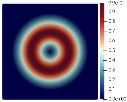
Figure 1: Gresho Vortex: Initial Mach number distribution $M/M_{r}$ for $M_{r}=3\times 10^{-3}$.

Figure 2 shows snapshots of the solution with each scheme at different Mach numbers, and provides a clear illustration of the accuracy degradation issues in the low-Mach regime (ES Roe). The other three schemes do not show a visible dependency on the reference Mach number. The best results are obtained with the EC flux. The difference between the ES Turkel and ES Miczek fluxes is not clearly visible from these plots.

(a) EC Roe $-M_{r}=3\times 10^{-1}$

(b) EC Roe $-M_{r}=3\times 10^{-2}$

(c) EC Roe $-M_{r}=3\times 10^{-3}$

(d) ES Miczek $-M_{r}=3\times 10^{-1}$

(e) ES Miczek $-M_{r}=3\times 10^{-2}$

(f) ES Miczek $-M_{r}=3\times 10^{-3}$

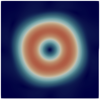
(g) ES Turkel $-M_{r}=3\times 10^{-1}$

(h) ES Turkel $-M_{r}=3\times 10^{-2}$

(i) ES Turkel $-M_{r}=3\times 10^{-3}$

(j) ES Roe $-M_{r}=3\times 10^{-1}$

(k) ES Roe $-M_{r}=3\times 10^{-2}$

(l) ES Roe $-M_{r}=3\times 10^{-3}$

Figure 2: Gresho Vortex: $M/M_{r}$ profiles at $t=1$. Same legend as figure 1-(a).

Figure 3 shows a normalized kinetic energy evolution for all four schemes at different Mach numbers. For the ES Roe flux, we see that the rate at which the kinetic energy decays increases with the Mach number. We can also see that the normalized kinetic energy for $M_{r}=3\times 10^{-2}$ becomes bigger than for $M_{r}=3\times 10^{-3}$. This was slightly visible in figure 2. The Gresho vortex is a stationary solution, hence it is not surprising that numerical solution would eventually reach a steady state (we could then see the faster kinetic energy decay as the scheme converging to a wrong solution faster as $M_{r}\xrightarrow{}0$). For the ES Miczek and ES Turkel fluxes, the kinetic energy decay appears to be independent of the Mach number. In each case, we see that the $M_{r}=3\times 10^{-1}$ curve is not matching exactly with the $M_{r}=\{3\times 10^{-2},\ 3\times 10^{-3}\}$ ones. We believe that this is because the $M_{r}=3\times 10^{-1}$ configuration does not completely fall into the incompressible regime. Figure 3 overall suggests that the ES Miczek flux performs better than the ES Turkel flux. This is also supported by figures 7(a)-(c)-(e) which show that the ES Turkel flux produces more entropy than the ES Miczek flux.

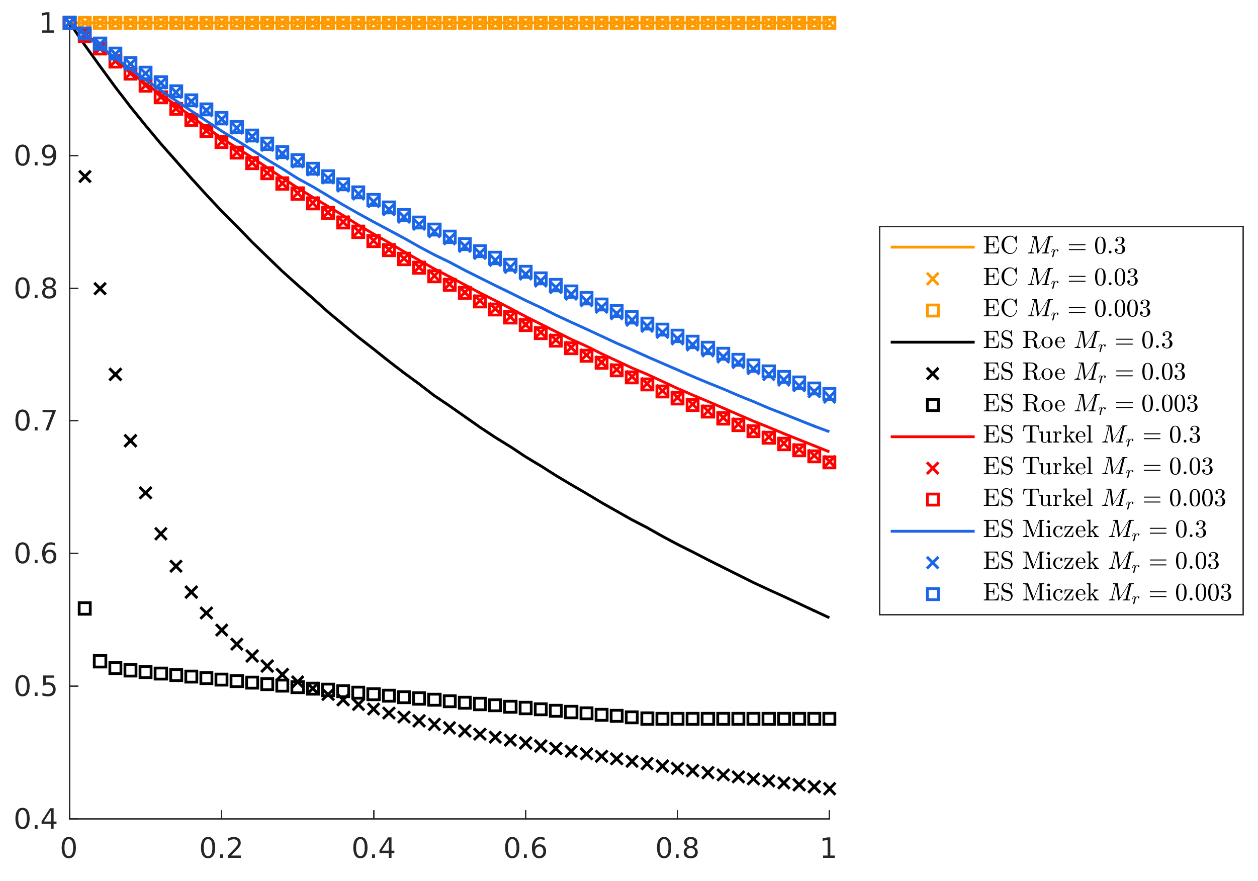
Figure 3: Gresho vortex: Total kinetic energy $k/k_{0}$ evolution over time for different ES fluxes at different Mach numbers.

Figure 4 shows the pressure distribution along the centerline $y=0.5$, after one revolution at $M_{r}=3\times 10^{-3}$. The solution with the ES Miczek flux is clearly not in phase with the exact solution. The same anomaly is observed at different Mach numbers. Figure 5 suggests that this anomaly is the consequence of a spurious transient in the early stages of the vortex rotation. We found that the duration of this transient decreases with the Mach number.

Figure 4: Gresho vortex: Centerline pressure profile $\hat{p}(x,0.5)$ after one rotation at $M_{r}=3\times 10^{-3}$.

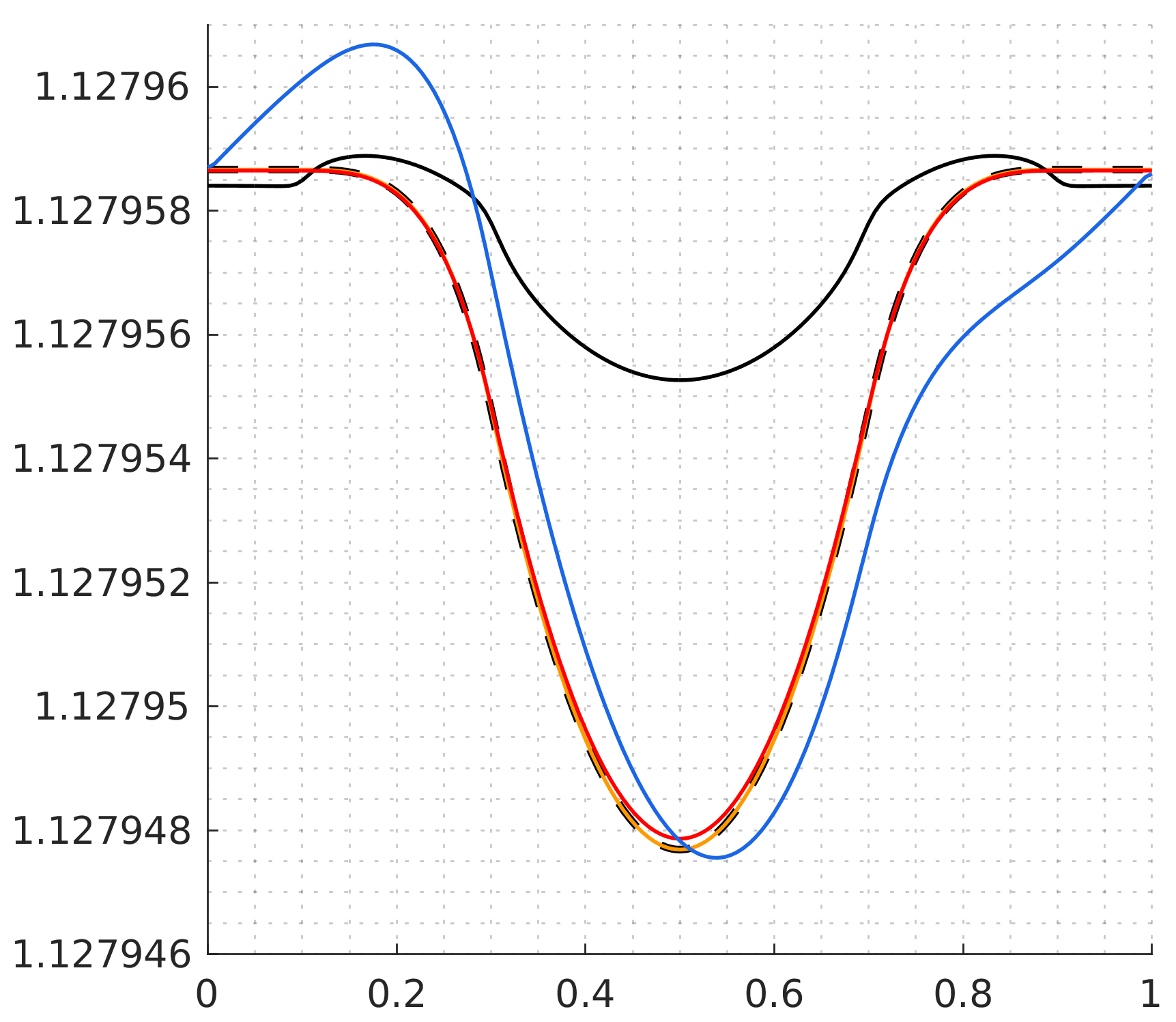
(a) $t=0.04$

(b) $t=0.08$

Figure 5: Gresho Vortex: Centerline pressure profiles at early instants highlighting the spurious transient observed with the ES Miczek flux (blue). $M_{r}=3\times 10^{-3}$. Same legend as figure 4.

5.2 Acoustic wave

One way to set up a right-moving acoustic wave is to consider, as in Bruel et al. Bruel , a free stream $(\rho_{\infty},u_{\infty},a_{\infty})$ and introduce fluctuations such that the Riemann invariants associated with the left moving acoustic wave and the entropy wave are constant throughout the domain. We set $\Omega=[-0.5,\ 0.5]$ and perturn density as follows:

$$\hat{\rho}(x,0)=\rho_{\infty}\big{(}1+M_{r}\psi(x)\big{)},$$

where $\psi(x)=\exp(-\alpha x^{2})$ defines a gaussian pulse centered at the center of the domain. We set $\alpha=\ln(10^{3})/0.15^{2}$ so that $\psi(x)<10^{-3}$ for $|x|<0.15$. The flow is isentropic, hence $\hat{p}(x,0)=\hat{\rho}(x,0)^{\gamma}\implies\hat{a}=\sqrt{\gamma}(\hat{\rho}(x,0))^{\frac{\gamma-1}{2}}$. The corresponding velocity perturbation must satisfy

$$\big{(}\hat{u}(x,0)-u_{\infty}\big{)}-\frac{2\big{(}\hat{a}(x,0)-a_{\infty}\big{)}}{\gamma-1}=0\ \implies\ \hat{u}(x,0)=u_{\infty}+\frac{2\big{(}\hat{a}(x,0)-a_{\infty}\big{)}}{\gamma-1}.$$

$\hat{a}(x,0)$ and $\hat{p}(x,0)$ are imposed by the density. If the reference Mach number $M_{r}$ is small enough, we can write:

$$\hat{u}(x,0)=u_{r}+\frac{2a_{r}}{\gamma-1}\bigg{(}\big{(}1+M_{r}\psi\big{)}^{\frac{\gamma-1}{2}}-1\bigg{)}=u_{\infty}+a_{\infty}M_{r}\psi+\mathcal{O}(M_{r}^{2}).$$ (73)

We set $u_{\infty}=0$ and $a_{\infty}=1$, so that the speed of propagation of the acoustic wave is roughly one. The reference time scale $t_{r}=1$ is the time it takes for the acoustic wave to do one period. We have $\rho_{r}=\rho_{\infty}$, $u_{r}=M_{r}$ and $a_{r}=a_{\infty}$. Hence, spatial fluctuations in $(\rho,p)$ are of order $M_{r}$, while fluctuations in $u$ are of order $1$.
We tested the four schemes on a grid of $500$ cells for $M_{r}\ \in\ \{10^{-2},\ 10^{-3},\ 10^{-4}\}$. Figures 6(a)-(c) show the numerical solution at $t=1$ for different Mach numbers. The reference solution is obtained using a 4-th order TecNO scheme ES_Fjordholm on a grid of $1000$ cells with a 4-th order Runge-Kutta time integration and a CFL of 0.5. We see that the ES Roe flux, ES Miczek flux and EC flux lead to a self-similar numerical solution. We can see that the acoustic wave is almost completely gone with the ES Turkel flux. This is in agreement with the analysis and results of Bruel et al. Bruel for the barotropic Euler equations. The ES Miczek flux does not have this problem. Furthermore, it seems to perform just as well as the EC flux. This is also supported by figures 7(b)-(d)-(f).

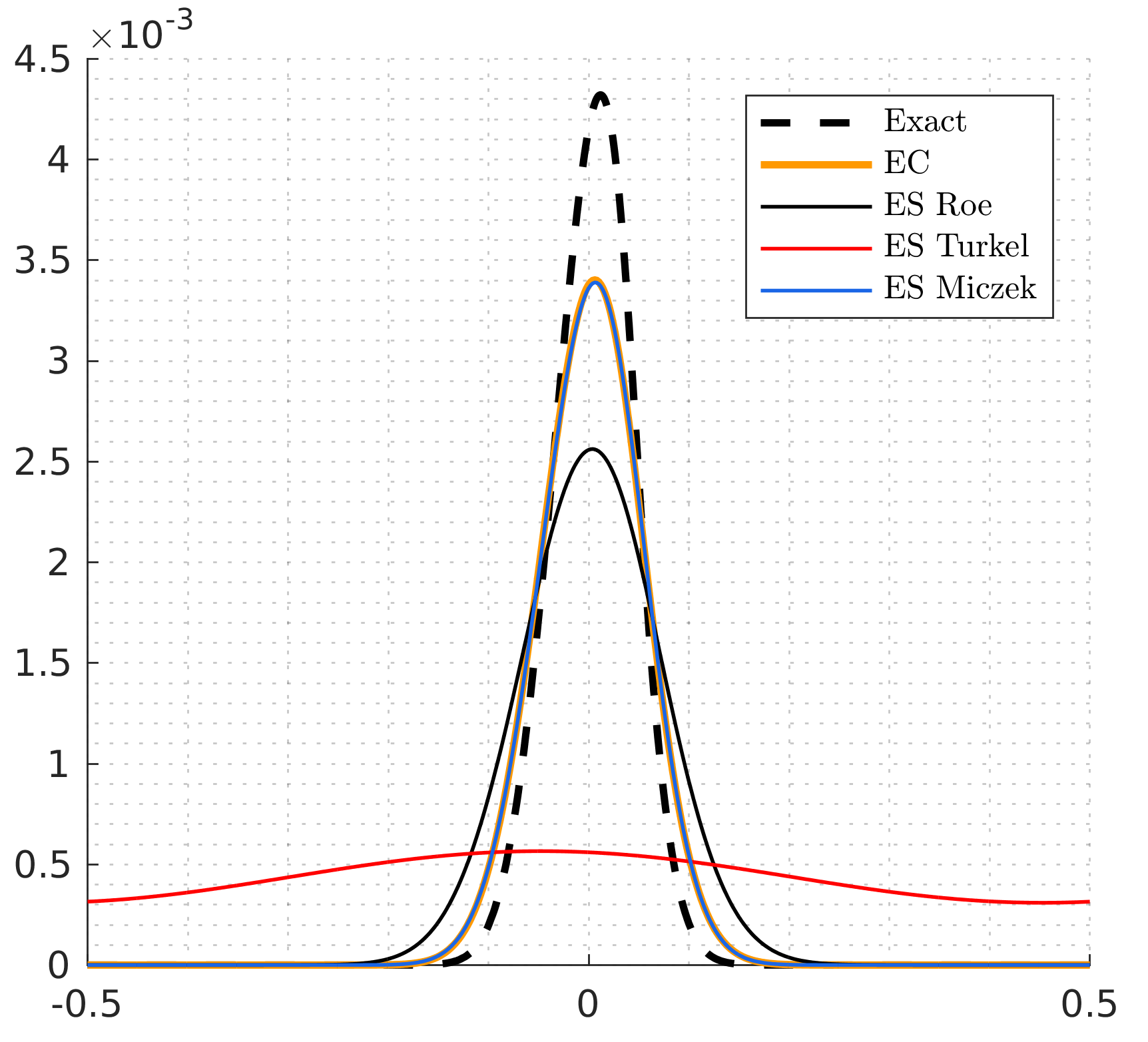
(a) $M_{r}=10^{-2}$

(b) $M_{r}=10^{-3}$

(c) $M_{r}=10^{-4}$

Figure 6: Sound wave: Pressure profiles at $t=1$ for different Mach numbers.

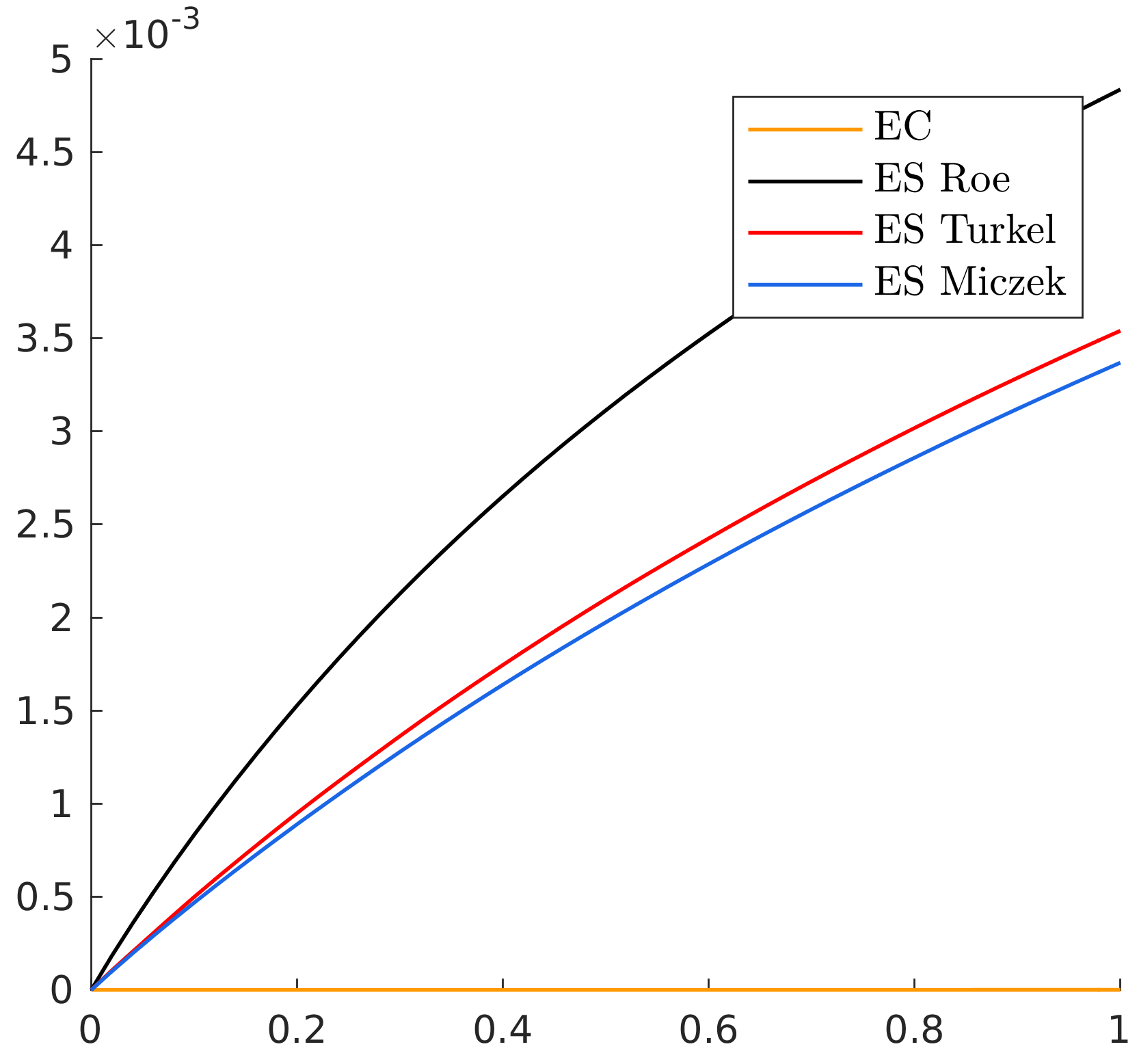
(a) Gresho Vortex - $M_{r}=3\times 10^{-1}$

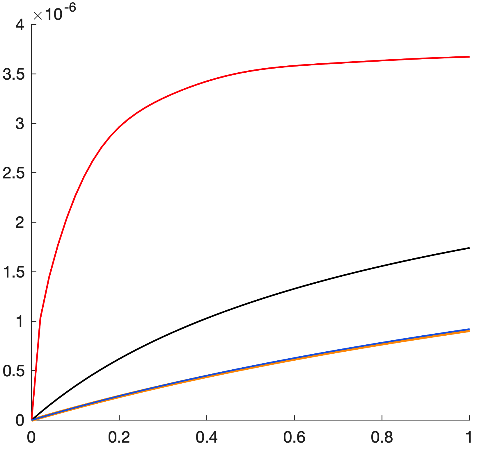
(b) Sound wave - $M_{r}=10^{-2}$

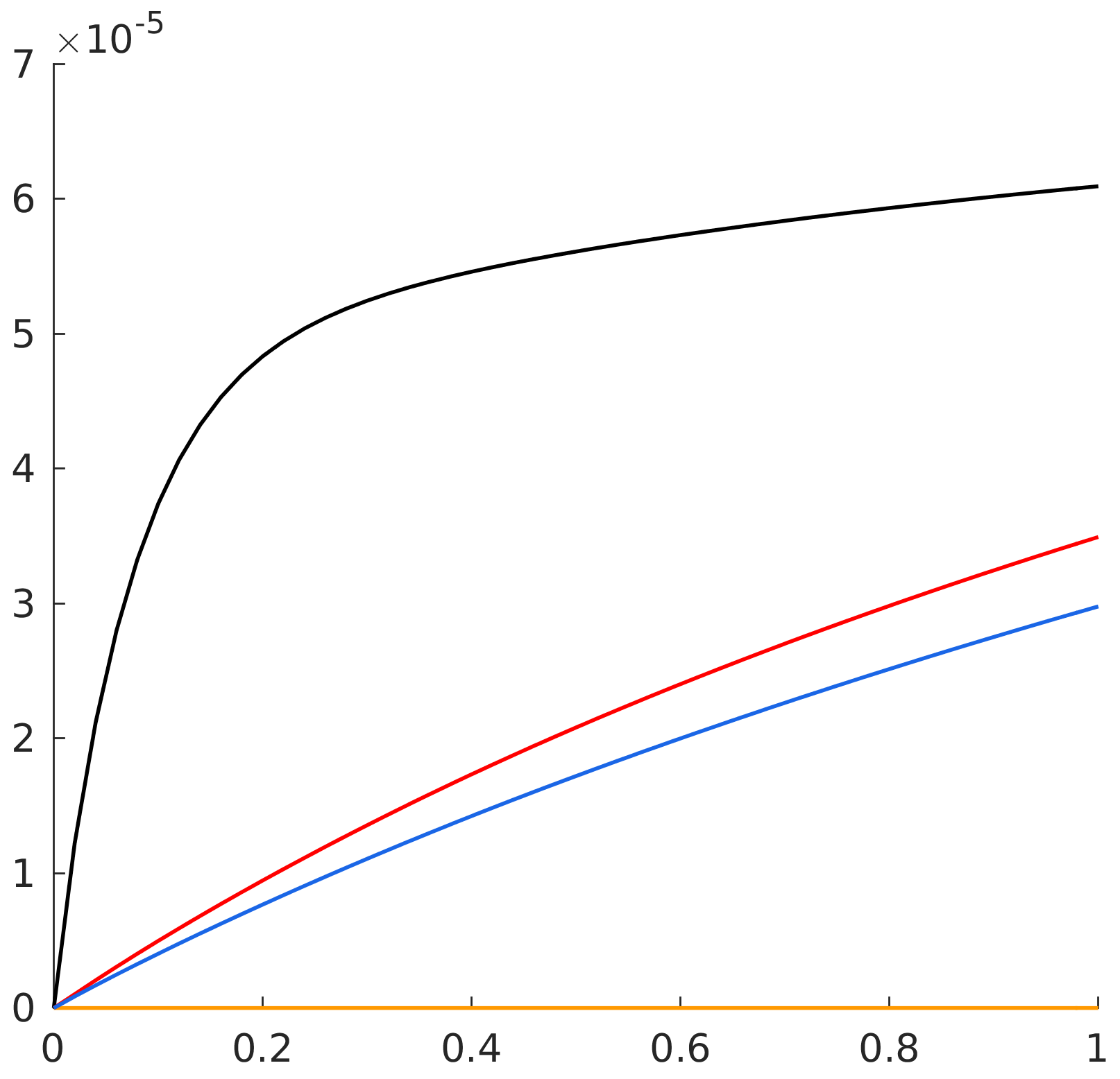
(c) Gresho Vortex - $M_{r}=3\times 10^{-2}$

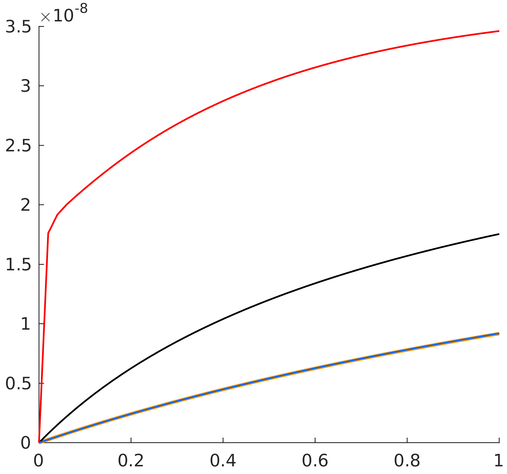
(d) Sound wave - $M_{r}=10^{-3}$

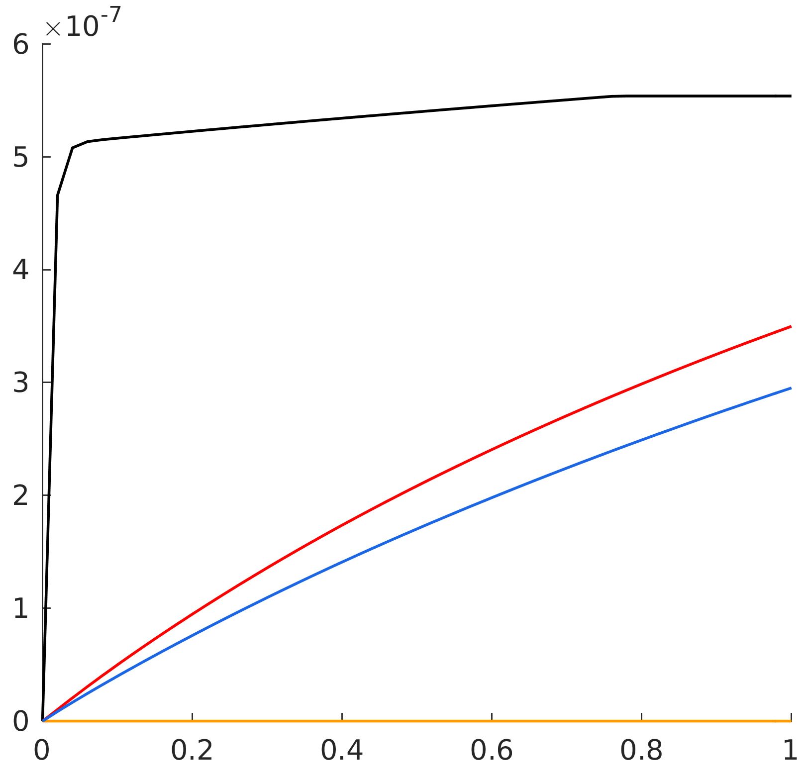
(e) Gresho Vortex - $M_{r}=3\times 10^{-3}$

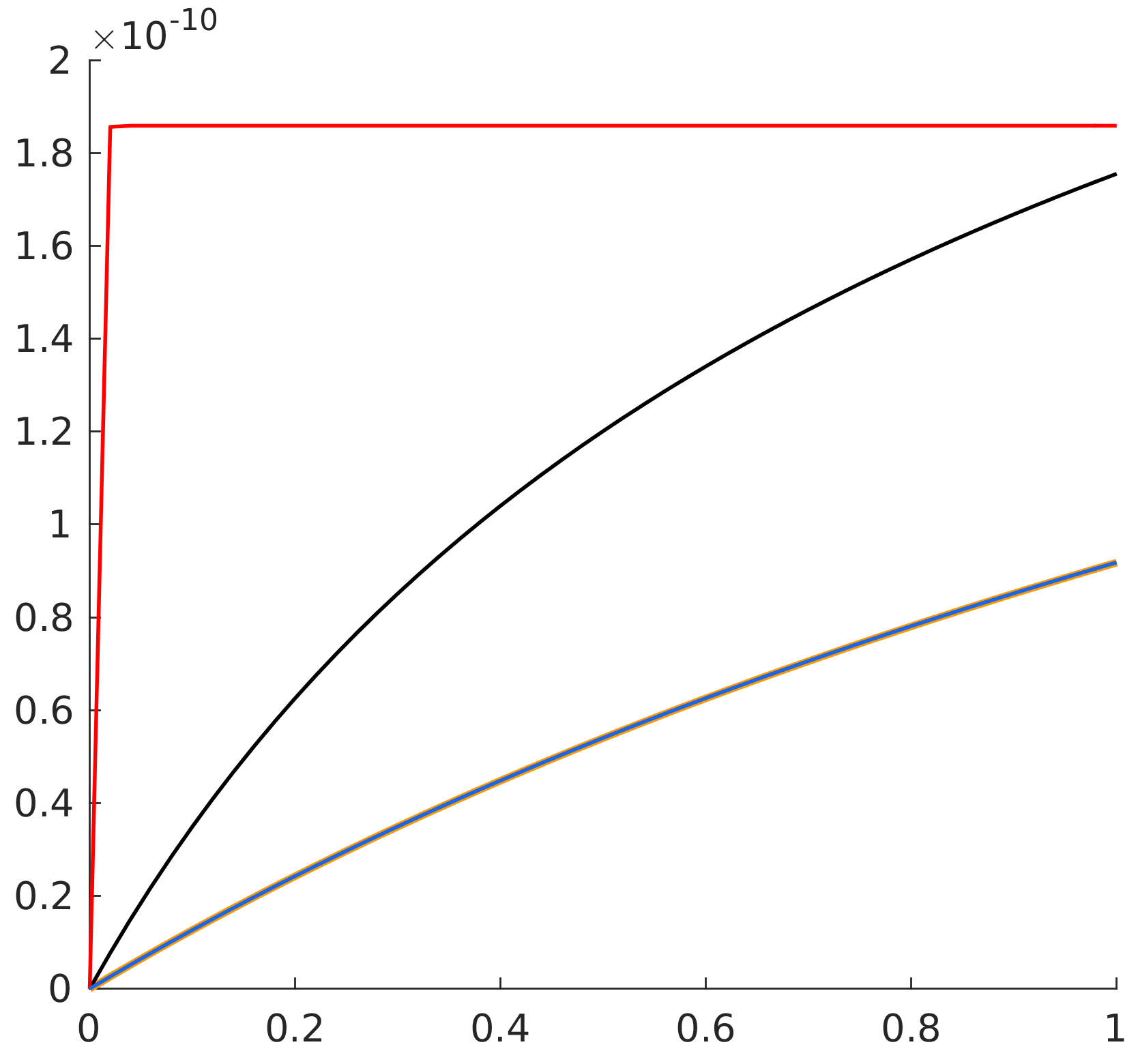
(f) Sound wave - $M_{r}=10^{-4}$

Figure 7: Total entropy $(\rho s)-(\rho s)_{0}$ over time for all fluxes for the Gresho Vortex (left) and the sound wave (right).

Figure 8 shows the temporal evolution of a normalized sound wave amplitude $A$ defined as:

$$A(t)=\frac{\max_{x\in\Omega}p(x,t)}{\max_{x\in\Omega}p(x,0)}.$$ (74)

We can see that the rate at which the ES Turkel flux damps the sound wave increases as the Mach number decreases, while all other fluxes show a self-similar behavior. For the ES Miczek flux, we notice slight perturbations in $A$ which seem to occur around $t=\{0,\ 0.5,\ 1.0\}$. Figure 9 suggests that these perturbations are caused by a spurious left-moving acoustic wave, created at $(x,t)=(0,0)$, that meets the right-moving acoustic wave when it reaches the periodic boundary and when it reaches the center of the domain at the end of the period.

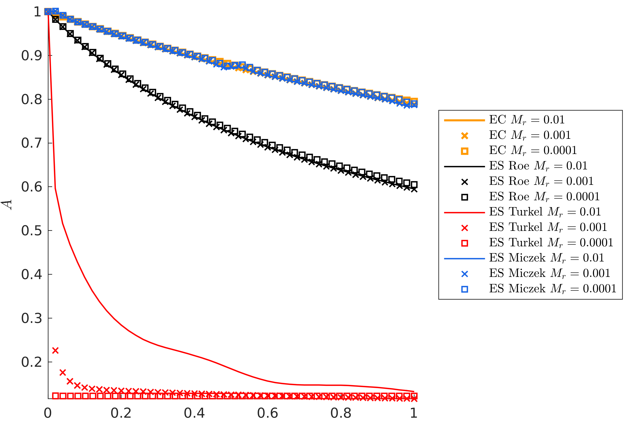
Figure 8: Sound wave: Normalized amplitude evolution for all fluxes at different Mach numbers.

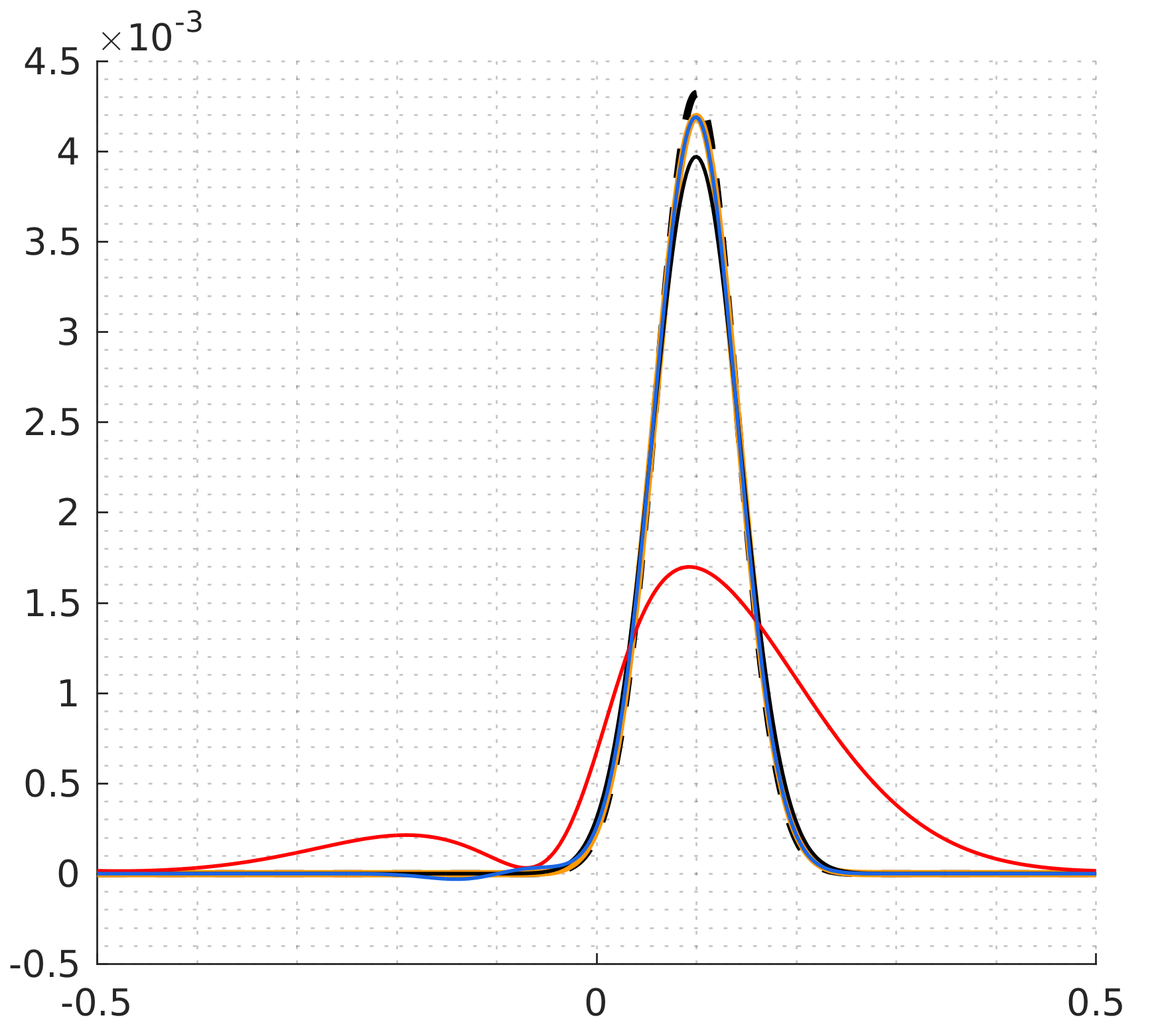
(a) $t=0.1$

(b) $t=0.1$ (zoom)

(c) $t=0.2$ (zoom)

(d) $t=0.3$ (zoom)

Figure 9: Sound wave: Pressure profiles showing that the spurious wave (blue) reported in figure 5 is an acoustic wave propagating at a speed of one. Same legend as figure 6(a).

5.3 Summary

At this point, we have demonstrated, both analytically and numerically, that Flux-Preconditioning is compatible with Entropy-Stability. Numerical results are overall consistent with previous studies:

1. The ES Roe flux suffers from the same accuracy issues in the incompressible low-Mach limit as those previously reported with the classic Roe flux Miczek_T ; Miczek ; Barsukow . This does not come as a surprise considering that the dissipation operators are not fundamentally different. These issues were not observed with the sound wave, in agreement with Bruel . The temporal variation of the wave amplitude (74) is independent of the Mach number.

2. The ES Turkel flux has a more consistent behavior in the incompressible limit, but at the price of damping acoustic waves harder as the Mach number decreases Bruel .

3. The ES Miczek flux performs well in both limits if we ignore the spurious transient in the Gresho vortex and the spurious left-moving acoustic wave, none of which were reported in Miczek_T ; Miczek ; Barsukow . These are hard to notice on contour plots.

The EC flux performs the best in both cases. This confirms that for standard ES schemes, it is the dissipation component of (52) that causes the accuracy issues. This also suggests that the simplest fix in the context of (implicit) ES schemes could be to simply discard the dissipation part of the ES flux. This will be investigated in future work for space-time high-order ES_Diosady discretizations in complex mixed flow configurations. We expect the stiffness issues associated with both the low-Mach regime and high-order implicit discretization to add a significant layer of complexity to the analysis.
What follows in the remaining two sections is entirely motivated by the authors’ goal to better understand the local behavior of ES schemes. The errors observed with the ES Miczek flux are intriguing. For the sound wave in particular, the spurious left-moving acoustic wave is reminiscent of anomalies the authors studied previously Gouasmi_0 ; Gouasmi_2 (none of which could be tied to the violation of an entropy inequality). For all these reasons, we decided to delve into these issues, with an emphasis on the physical quantity ES schemes have an actual handle on.

6 The Accuracy Degradation from an Entropy Production Perspective

In the incompressible limit, Guillard & Viozat Guillard1 showed that pressure fluctuations in space are of order $M^{2}$, i.e. we can write $p(\mathbf{x},t)=p_{0}(t)+M^{2}p_{2}(\mathbf{x},t)$. Assuming constant density $\rho=\rho_{0}$, we can write:

$$\rho s= \ \rho_{0}\bigg{(}\ln\big{(}p_{0}+M_{r}^{2}p_{2}+\mathcal{O}(M_{r}^{3})\big{)}-\gamma\ln(\rho_{0})\bigg{)}=\rho_{0}\bigg{(}s_{0}+\ln\big{(}1+M_{r}^{2}(p_{2}/p_{0})+\mathcal{O}(M_{r}^{3})\big{)}\bigg{)}=\rho_{0}s_{0}+M_{r}^{2}\rho_{0}(p_{2}/p_{0})+\mathcal{O}(M_{r}^{3}).$$

with $s_{0}=\ln p_{0}-\gamma\ln\rho_{0}$. Therefore, we state:

1. In the incompressible limit, entropy $\rho s$ fluctuations in space should be of order $M_{r}^{2}$.

Similarly Guillard2 :

1. In the acoustic limit, entropy $\rho s$ fluctuations in space should be of order $M_{r}$.

In the incompressible limit, there is the additional requirement that kinetic energy should be conserved. To precisely and rigorously relate discrete changes in kinetic energy to discrete changes in entropy is not straightforward, if at all possible. Let’s assume periodic boundary conditions so that discrete conservation of total energy implies that it remains constant globally. We can write:

$$\Delta(\rho e+M_{r}^{2}\rho k)=0\ \iff\ \Delta(\rho k)=-\frac{1}{M_{r}^{2}}\Delta(\rho e)=-\frac{1}{(\gamma-1)M_{r}^{2}}\Delta(p)=-\frac{1}{(\gamma-1)M_{r}^{2}}\Delta\bigg{(}\exp\bigg{(}\frac{\rho s-\gamma\rho\ln(\rho)}{\rho}\bigg{)}\bigg{)},$$

where $\Delta$ refers to the global change, that is the sum $\sum_{i}\Delta_{i}$ of local changes in each cell $i$. Assuming constant density, this relation simplifies to:

$$\Delta(\rho k)=\frac{-1}{\exp(\rho)(\gamma-1)M_{r}^{2}}\Delta\big{(}\exp(\rho s)\big{)}.$$ (75)

Equation (75) relates the global change in kinetic energy $\rho k$ to the global change in the exponential of the entropy, which ES schemes do not explicitly control. It is certainly tempting to say that since the exponential function is monotonically increasing, $\Delta(\rho s)>0\implies\Delta\big{(}\exp(\rho s)\big{)}>0$. This statement is true locally, but ES schemes are not explicitly designed to achieve $\Delta_{i}(\rho s)>0$, because equation (53) also features flux contributions (in other words, one could have $\Delta_{i}(\rho s)<0$). We therefore refrain from making hasty interpretations.

6.1 Entropy Production Breakdowns (EPBs)

The most remarkable feature of ES schemes is the relation that holds at the semi-discrete level for entropy in each cell (53), which we rewrite here:

$$\frac{dU(\mathbf{u}_{i})}{dt}\ +\ \frac{1}{V_{i}}\int_{\delta\Omega_{i}}F^{*}dS\ =\ -\frac{1}{V_{i}}\mathcal{E}_{i},\ \mathcal{E}_{i}=\int_{\delta\Omega_{i}}\mathcal{E}dS.$$

The cell valued field $\mathcal{E}_{i}$ tells us how much entropy is produced in space in response to the jumps in entropy variables across interfaces. It can therefore give us an idea of the magnitude of the entropy fluctuations the scheme creates. To this end, we proceed to derive a more detailed expression for $\mathcal{E}$. Ignoring the $1/4$ factor in (55), we have:

$$\mathcal{E}\ =\ [\mathbf{v}]^{T}D[\mathbf{v}]\ =\ [\mathbf{v}]^{T}R|\Lambda|R^{T}[\mathbf{v}].$$

Now let $\mathbf{r}_{1},\ \dots,\mathbf{r}_{N}$ denote the columns of the eigenvector matrix $R$ where $N$ is the number of eigenvalues (possibly repeated). We have $R=[\mathbf{r}_{1},\ \dots\ ,\mathbf{r}_{N}]$, $|\Lambda|=diag(|\lambda_{1}|,\ \dots\,|\lambda_{N}|)$. Define $\bm{\mu}^{T}=[\mu_{1},\ \dots,\ \mu_{N}]=[\mathbf{v}]^{T}R$. We have:

$$\mathcal{E}\ =\ \bm{\mu}^{T}|\Lambda|\bm{\mu}\ =\ \sum_{k=1}^{N}|\lambda_{k}|\mu_{k}^{2},$$

and we can see how the total entropy production breaks down into the positive contributions associated with each eigenvector or ”mode” $\mathbf{r_{i}}$. This decomposition is inspired by how Roe & Pike Pike rewrote the Roe flux:

$$R|\Lambda|R^{-1}[\mathbf{u}]\ =\ \sum_{k=1}^{N}|\lambda_{k}|\alpha_{k}\mathbf{r_{k}},\ \bm{\alpha}=R^{-1}[\mathbf{u}].$$ (76)

It is also inspired by the family of closed-form EC fluxes Tadmor proposed in ES_Tadmor_2003 (we discuss them in section 7).
The vector $\bm{\alpha}$ in equation (76) is known as a vector of wave strengths. We can interpret $\bm{\mu}=R^{T}[\mathbf{v}]$ in our decomposition as a vector of wave strengths as well, as for infinitesimal variations we have:

$$d\mathbf{u}=Hd\mathbf{v}=RR^{T}d\mathbf{v}\implies R^{-1}d\mathbf{u}=R^{T}d\mathbf{v}.$$

For the compressible Euler system (2.2), $R=[\mathbf{r}_{u_{n},1},\ \mathbf{r}_{u_{n},2},\ \mathbf{r}_{u_{n},3},\ \mathbf{r}_{u_{n}+a},\ \mathbf{r}_{u_{n}-a}]$ ($N=5$) and we have:

$$\mathcal{E}=|u_{n}|(\mu_{u_{n},1}^{2}+\mu_{u_{n},2}^{2}+\mu_{u_{n},3}^{2})+|u_{n}+(a/M_{r})|\mu_{u_{n}+a}^{2}+|u_{n}-(a/M_{r})|\mu_{u_{n}-a}^{2}.$$ (77)

It breaks down into entropy production due to convective modes (first three terms, which we gather into $\mathcal{E}_{u_{n}}$) and entropy production due to acoustic modes (remaining two terms, which we denote $\mathcal{E}_{u_{n}+a}$ and $\mathcal{E}_{u_{n}-a}$ respectively). We expect the latter to be the key in understanding the low-Mach problems. The entropy production field $\hat{\mathcal{E}}$ that the code solving the dimensional system (2) computes is related to $\mathcal{E}$ by the simple relation:

$$\hat{\mathcal{E}}=(\rho_{r}u_{r})\times\mathcal{E}.$$ (78)

Given that in both test problems the reference Mach number $M_{r}$ is adjusted by changing the the reference velocity $u_{r}$ only, we use $\hat{\mathcal{E}}=M_{r}\times\mathcal{E}$ instead. We also define the global quantity (sum over all cells):

$$\langle\mathcal{E}\rangle=\sum_{i}\mathcal{E}_{i},$$ (79)

which we will subsequently use to visualize the global influence of each entropy production field in (77) on the total entropy production in space.
We now proceed to develop the expressions of $\mathcal{E}_{u_{n}},\mathcal{E}_{u_{n}-a}$ and $\mathcal{E}_{u_{n}+a}$. We will first treat the convective modes (entropy & shear waves) since they are common to all three ES fluxes. We then treat the acoustic modes. Note that these dissipation matrices are evaluated at averaged states (we simply take arithmetic averages for all ES fluxes). For smooth flow configurations, we do not expect the choice of average values to have a impact.

Convective modes. The scaled eigenvectors associated with $\lambda=u_{n}$ are given by:

$$\mathbf{r}_{u_{n},1}=K_{q}(n_{1}K_{0}\mathbf{r_{0}}+(a/M_{r})\mathbf{r_{s1}}),\ \mathbf{r}_{u_{n},2}=K_{q}(n_{2}K_{0}\mathbf{r_{0}}+(a/M_{r})\mathbf{r_{s2}}),\ \mathbf{r}_{u_{n},3}=K_{q}(n_{3}K_{0}\mathbf{r_{0}}+(a/M_{r})\mathbf{r_{s3}}),$$

$$\mathbf{r_{0}}=\begin{bmatrix}1\\ u\\ v\\ w\\ M_{r}^{2}k\end{bmatrix},\mathbf{r_{s1}}=\begin{bmatrix}0\\ 0\\ n_{3}\\ -n_{2}\\ M_{r}^{2}(n_{3}v-n_{2}w)\end{bmatrix},\mathbf{r_{s2}}=\begin{bmatrix}0\\ -n_{3}\\ 0\\ n_{1}\\ M_{r}^{2}(n_{1}w-n_{3}u)\end{bmatrix},\ \mathbf{r_{s3}}=\begin{bmatrix}0\\ n_{2}\\ -n_{1}\\ 0\\ M_{r}^{2}(n_{2}u-n_{1}v)\end{bmatrix},$$

$$K_{q}=(\rho/\gamma)^{1/2},\ K_{0}=(\gamma-1)^{1/2}.$$

$\mathbf{r_{0}}$ is an entropy wave. Let $\mu_{0}=\mathbf{r_{0}}^{T}[\mathbf{v}]$ be the corresponding wave strength, we can show that:

$$\mu_{0}= \ \frac{-[s]}{\gamma-1}-\frac{M_{r}^{2}}{4}\bigg{[}\frac{\rho}{p}\bigg{]}\bigg{(}[u]^{2}+[v]^{2}+[w]^{2}\bigg{)}.$$

$\mathbf{r_{s1}},\mathbf{r_{s2}}$ and $\mathbf{r_{s3}}$ are shear waves (they satisfy $n_{1}\mathbf{r_{s1}}+n_{2}\mathbf{r_{s2}}+n_{3}\mathbf{r_{s3}}=0$). The corresponding wave strengths $\mu_{s1}=\mathbf{r_{s1}}^{T}[\mathbf{v}],\ \mu_{s2}=\mathbf{r_{s2}}^{T}[\mathbf{v}]$ and $\mu_{s3}=\mathbf{r_{s3}}^{T}[\mathbf{v}]$ are given by:

$$\mu_{s1}=M_{r}^{2}\overline{\bigg{(}\frac{\rho}{p}\bigg{)}}[\mathcal{V}_{1}],\ \mu_{s2}=M_{r}^{2}\overline{\bigg{(}\frac{\rho}{p}\bigg{)}}[\mathcal{V}_{2}],\ \mu_{s3}=M_{r}^{2}\overline{\bigg{(}\frac{\rho}{p}\bigg{)}}[\mathcal{V}_{3}],$$

$$\mathcal{V}_{1}=n_{3}v-n_{2}w,\ \mathcal{V}_{3}=n_{1}w-n_{3}u,\ \mathcal{V}_{3}=n_{2}u-n_{1}v.$$

We now have:

$$\mathcal{E}_{u_{n}}= \ |u_{n}|K_{q}^{2}\bigg{(}\ (n_{1}K_{0}\mu_{0}+(a/M_{r})\mu_{s1})^{2}\ +\ (n_{2}K_{0}\mu_{0}+(a/M_{r})\mu_{s2})^{2}\ +\ (n_{3}K_{0}\mu_{0}+(a/M_{r})\mu_{s3})^{2}\ \bigg{)}$$

$$= \ |u_{n}|K_{q}^{2}\bigg{(}\ K_{0}^{2}\mu_{0}^{2}\ +\ (a/M_{r})^{2}(\mu_{s1}^{2}+\mu_{s2}^{2}+\mu_{s3}^{2})\ \bigg{)}$$

$$= \ |u_{n}|\bigg{(}\ \frac{(\gamma-1)}{\gamma}\rho\mu_{0}^{2}\ +\ \frac{\rho a^{2}}{\gamma M_{r}^{2}}(\mu_{s1}^{2}+\mu_{s2}^{2}+\mu_{s3}^{2})\bigg{)}.$$

Injecting the discrete wave strength expressions, we get:

$$\mathcal{E}_{u_{n}}=|u_{n}|\bigg{(}\ \frac{\gamma-1}{\gamma}\rho\mu_{0}^{2}\ +\ \alpha\rho M_{r}^{2}([\mathcal{V}_{1}]^{2}+[\mathcal{V}_{2}]^{2}+[\mathcal{V}_{3}]^{2})\bigg{)},\ \alpha=\frac{a^{2}}{\gamma}\overline{\bigg{(}\frac{\rho}{p}\bigg{)}}^{2},$$ (80)

which we rewrite as the sum of a contribution of an entropy wave contribution $\mathcal{E}_{u_{n},s}$ (first term) and a contribution due to shear waves $\mathcal{E}_{u_{n},\tau}$ (remaining three terms).

$$\mathcal{E}_{u_{n}}=\mathcal{E}_{u_{n},s}+\mathcal{E}_{u_{n},\tau}.$$

For cartesian grids aligned with the $(x,y,z)$ coordinate system, the normal vectors are along the basis vectors and the entropy production due to shear $\mathcal{E}_{u_{n},\tau}$ can be broken down into 6 terms:

• Along $x$, shear in y ($\mathcal{E}_{u_{n},\tau_{xy}}=|u_{n}|\mu_{3}^{2}$) and shear in z ($\mathcal{E}_{u_{n},\tau_{xz}}=|u_{n}|\mu_{2}^{2}$).

• Along $y$, shear in z ($\mathcal{E}_{u_{n},\tau_{yz}}=|u_{n}|\mu_{1}^{2}$) and shear in x ($\mathcal{E}_{u_{n},\tau_{yx}}=|u_{n}|\mu_{3}^{2}$).

• Along $z$, shear in y ($\mathcal{E}_{u_{n},\tau_{zy}}=|u_{n}|\mu_{1}^{2}$) and shear in x ($\mathcal{E}_{u_{n},\tau_{zx}}=|u_{n}|\mu_{2}^{2}$).

This gives:

$$\mathcal{E}_{u_{n},\tau}\ =\ \mathcal{E}_{u_{n},\tau_{xy}}+\mathcal{E}_{u_{n},\tau_{xz}}+\mathcal{E}_{u_{n},\tau_{yx}}+\mathcal{E}_{u_{n},\tau_{yz}}+\mathcal{E}_{u_{n},\tau_{zx}}+\mathcal{E}_{u_{n},\tau_{zy}}$$ (81)

Acoustic modes. The scaled acoustic eigenvectors $\mathbf{r}_{4,5}=\mathbf{r}_{u_{n}\pm a}$ are given by :

$$\mathbf{r}_{u_{n}\pm a}=K_{a}\begin{bmatrix}1\\ u\pm n_{1}(a/M_{r})\\ v\pm n_{2}(a/M_{r})\\ w\pm n_{3}(a/M_{r})\\ h+M_{r}^{2}k\pm u_{n}aM_{r}\end{bmatrix},\ K_{a}=\bigg{(}\frac{\rho}{2\gamma}\bigg{)}^{1/2}.$$

The acoustic wave strengths $\mu_{u_{n}\pm a}=\mathbf{r}_{u_{n}\pm a}[\mathbf{v}]$ are given by:

$$\mu_{u_{n}\pm a}=K_{a}\bigg{(}\mu_{0}\ -\ h\bigg{[}\frac{\rho}{p}\bigg{]}\ \pm\ M_{r}a\overline{\bigg{(}\frac{\rho}{p}\bigg{)}}[u_{n}]\bigg{)}.$$

The entropy production field due to acoustic modes therefore writes:

$$\mathcal{E}_{u_{n}\pm a}=|u_{n}\pm(a/M_{r})|K_{a}^{2}\bigg{(}\mu_{0}\ -\ h\bigg{[}\frac{\rho}{p}\bigg{]}\ \pm\ M_{r}a\overline{\bigg{(}\frac{\rho}{p}\bigg{)}}[u_{n}]\bigg{)}^{2}.$$

Summary. Overall, the discrete entropy production field $\mathcal{E}=[\mathbf{v}]^{T}D[\mathbf{v}]$ can be decomposed as:

$$\mathcal{E}\ =\ \mathcal{E}_{u_{n},s}\ +\ \big{(}\mathcal{E}_{u_{n},\tau_{xy}}+\mathcal{E}_{u_{n},\tau_{xz}}+\mathcal{E}_{u_{n},\tau_{yx}}+\mathcal{E}_{u_{n},\tau_{yz}}+\mathcal{E}_{u_{n},\tau_{zx}}+\mathcal{E}_{u_{n},\tau_{zy}}\big{)}\ +\ \mathcal{E}_{u_{n}+a}\ +\ \mathcal{E}_{u_{n}-a}$$ (82)

Each of these entropy production fields can be visualized. Figures 10 and 11 show them for the Gresho vortex at $t=0$. This is, to the best of our knowledge, the first time that a concrete view on how an ES scheme produces entropy locally is given. What is striking is that the acoustic entropy production fields are 2 to 5 orders of magnitudes bigger than the convective ones. Figures 13(a)-(b)-(e) show that the acoustic entropy production fields make for most of the entropy produced by the ES Roe flux.
Similarly, figures 12(a)-(c) show the entropy production fields at $t=0$ for the acoustic wave. The entropy production field associated with entropy waves (there is no shear in this one-dimensional setup) and the entropy production field associated with left-moving acoustic waves are negligible compared to the entropy production field associated with right-moving acoustic waves. This makes sense, and over time, this difference in magnitude is sustained as shown in figures 13(b)-(d)-(f).

(a) $\hat{\mathcal{E}}_{u_{n},\tau_{xy}}$

(b) $\hat{\mathcal{E}}_{u_{n},\tau_{yx}}$

(c) $\hat{\mathcal{E}}_{u_{n},s}$

Figure 10: Gresho vortex: Entropy production fields associated with the convective modes at $t=0$ and $M_{r}=3\times 10^{-2}$. These are common to all ES fluxes.

(a) $\hat{\mathcal{E}}_{u_{n}+a}$

(b) $\hat{\mathcal{E}}_{u_{n}-a}$

Figure 11: Gresho vortex: Acoustic Entropy production fields at $t=0$ of the ES Roe flux at $M_{r}=3\times 10^{-2}$.

(a) $\hat{\mathcal{E}}_{u_{n}+a}$

(b) $\hat{\mathcal{E}}_{u_{n}-a}$

(c) $\hat{\mathcal{E}}_{u_{n},s}$

Figure 12: Sound Wave: Entropy production fields at different Mach numbers at $t=0$ and $M_{r}=10^{-2}$ for the ES Roe flux.

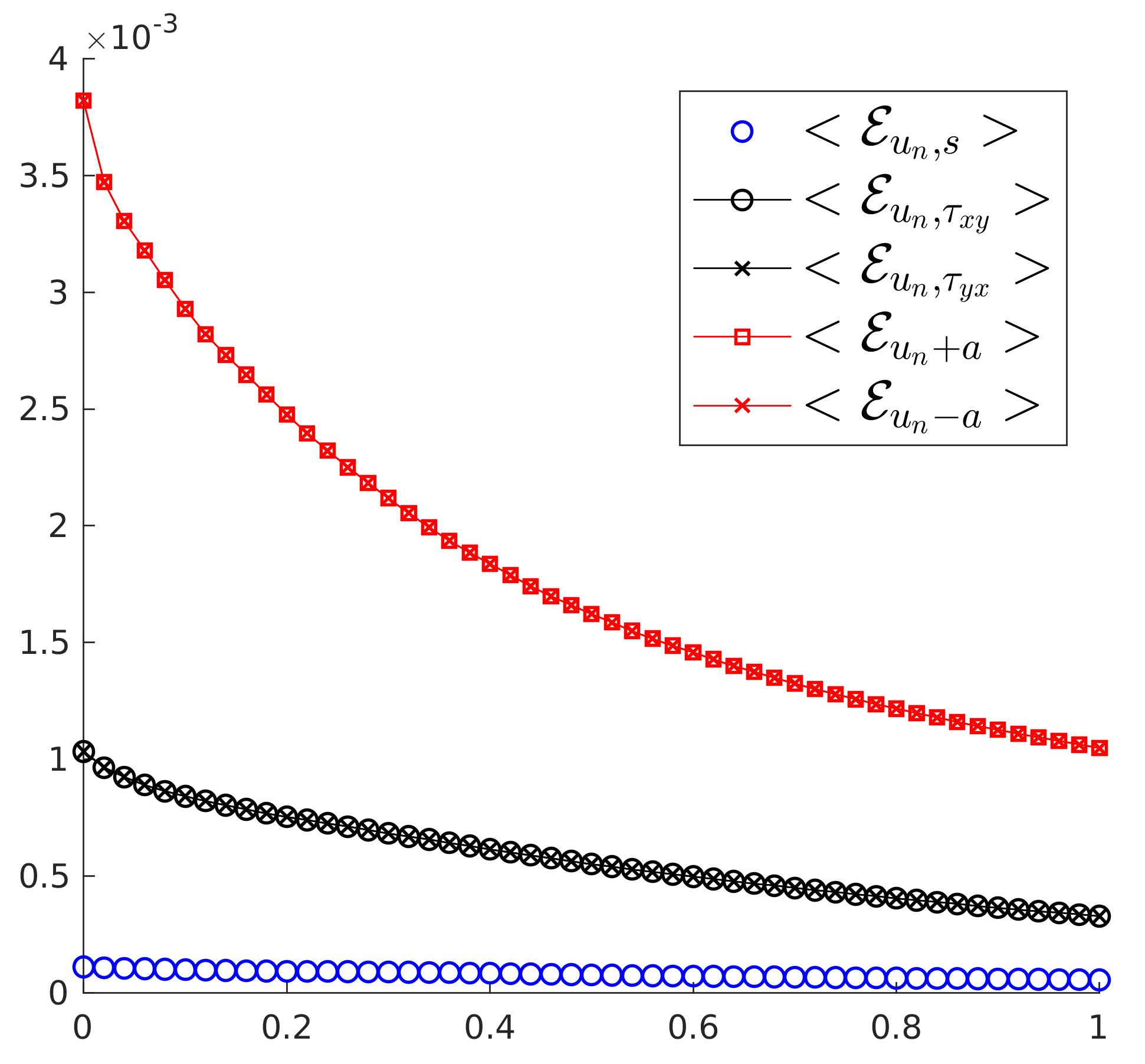
(a) Gresho Vortex - $M_{r}=3\times 10^{-1}$

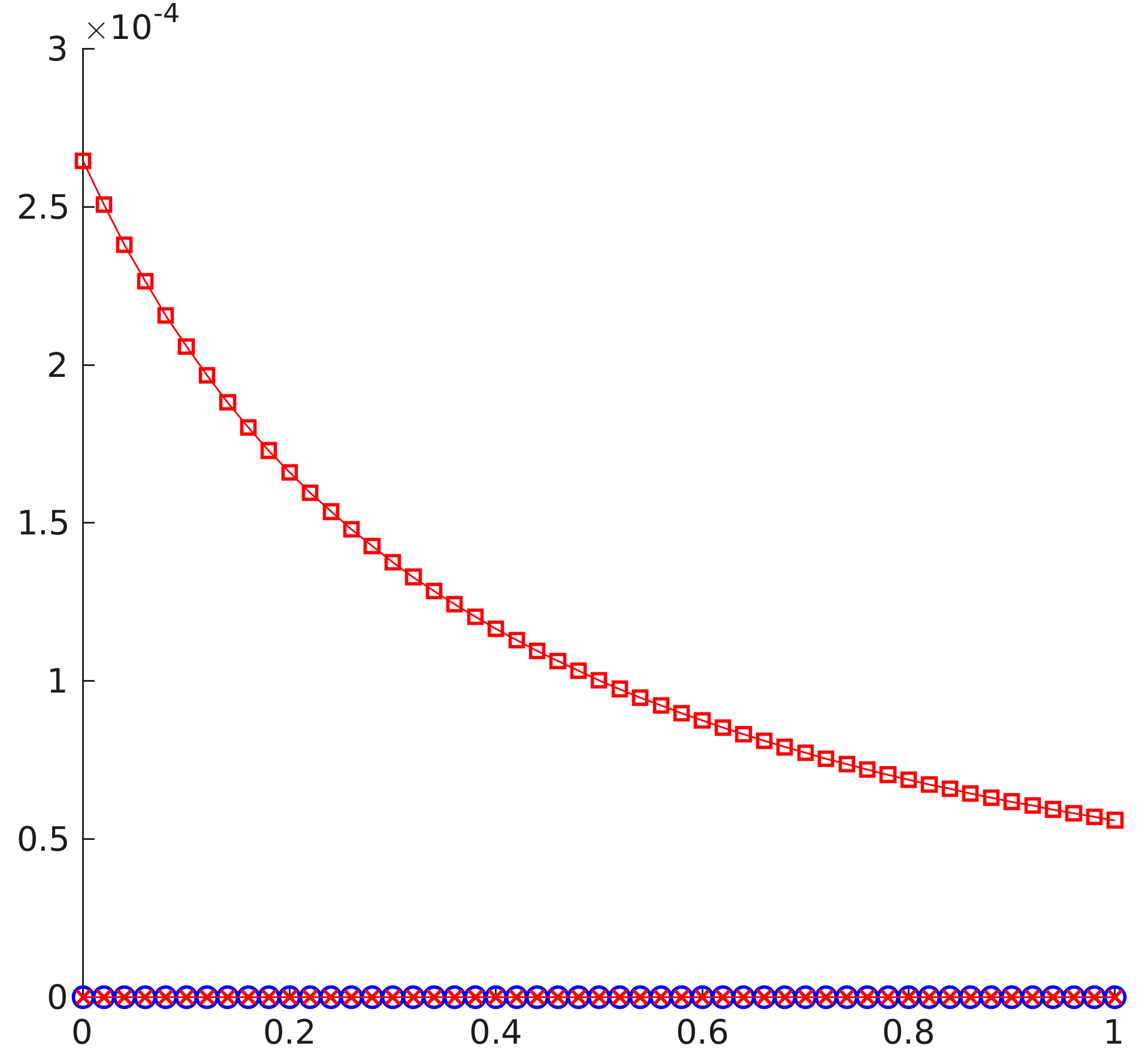
(b) Sound Wave - $M_{r}=10^{-2}$

(c) Gresho Vortex - $M_{r}=3\times 10^{-2}$

(d) Sound Wave - $M_{r}=10^{-3}$

(e) Gresho Vortex - $M_{r}=3\times 10^{-3}$

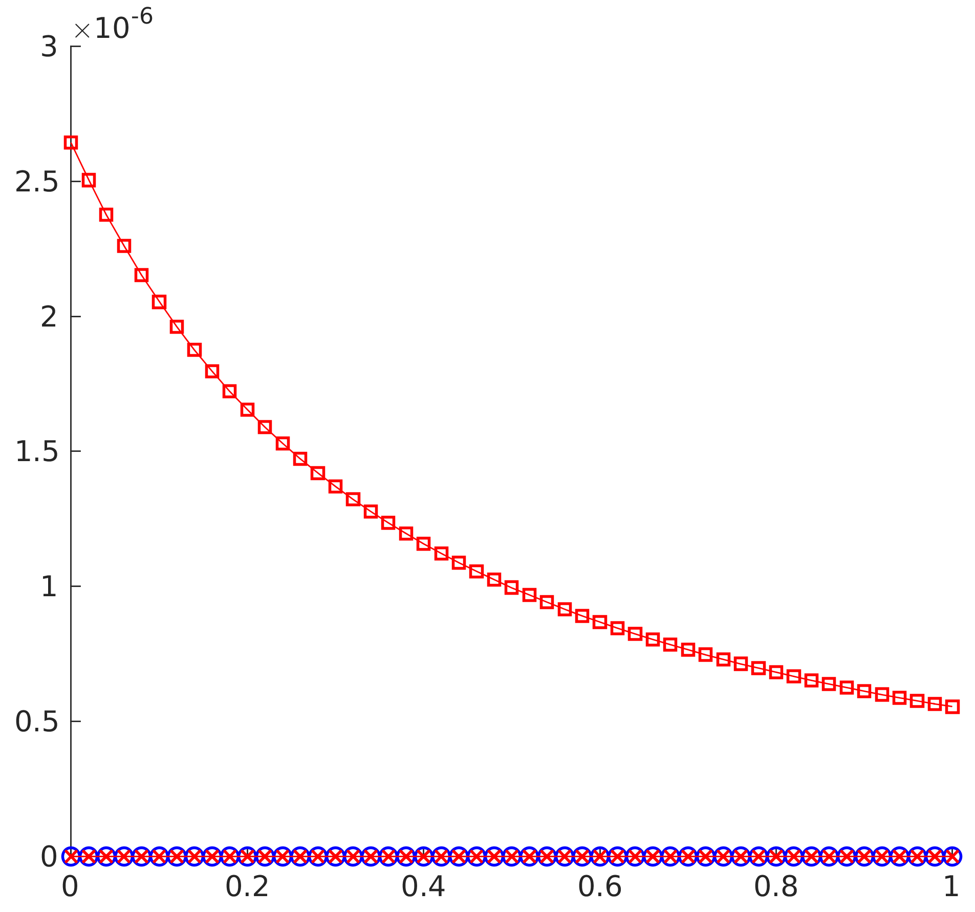
(f) Sound Wave - $M_{r}=10^{-4}$

Figure 13: Integral of each entropy production field with time at different Mach numbers for the ES Roe flux on the Gresho Vortex (left) and the sound wave (right).

6.1.1 EPBs of Preconditioned operators

EPBs for the preconditioned operators $D_{P}[\mathbf{v}]$ of Turkel and Miczek can be obtained if we manage to express them in a symmetric form $R|\Lambda|R^{T}[\mathbf{v}]$. For this purpose, we can start from the congruence relation (69) we established in section 4:

$$P^{-1}|PA|[\mathbf{v}]\ =\ (QH_{\mathbf{z}}^{1/2}P_{\mathbf{z}}^{-1})\ (|P_{\mathbf{z}}A_{\mathbf{z}}|P_{\mathbf{z}}^{T})\ (QH_{\mathbf{z}}^{1/2}P_{\mathbf{z}}^{-1})^{T}.$$

We see that a symmetric form for $D_{P}$ can be inferred from one for $|P_{\mathbf{z}}A_{\mathbf{z}}|P_{\mathbf{z}}^{T}$ (and vice versa). A simple trick to proceed, which we picked up from Diosady & Murman ES_Diosady , consists in forcing the eigenscaling theorem (4.4) by introducing the matrix $T^{2}_{p}$ defined by $P_{\mathbf{z}}^{T}=R_{p\mathbf{z}}T_{p}^{2}R_{p\mathbf{z}}^{T}$. From there, we have:

$$|P_{\mathbf{z}}A_{\mathbf{z}}|P_{\mathbf{z}}^{T}=R_{p\mathbf{z}}|\Lambda_{p}|T_{p}^{2}R_{p\mathbf{z}}^{T}\ \implies\ D_{P}=R_{p}(|\Lambda_{p}|T_{p})R_{p}^{T},\ R_{p}=QH_{\mathbf{z}}^{1/2}P_{\mathbf{z}}^{-1}R_{p\mathbf{z}}.$$ (83)

If $T_{p}$ is diagonal, an EPB can be introduced along the column vectors of $R_{p}$. Turkel’s matrix qualifies with $T_{p}^{2}$ given by:

$$T_{p}^{2}=diag([1,\ 1,\ 1,\ K_{2}^{2}+p^{2},\ K_{1}^{2}+p^{2}]),$$ (84)

and $R_{p}=[\mathbf{r}_{u_{n},1},\ \mathbf{r}_{u_{n},2},\ \mathbf{r}_{u_{n},3},\ \mathbf{r}_{u_{np}+a_{p}},\ \mathbf{r}_{u_{np}-a_{p}}]$ with:

$$\mathbf{r}_{u_{np}+a_{p}}=\sqrt{\frac{\rho}{\gamma}}\frac{K_{1}}{p^{2}(K_{1}-K_{2})}\begin{bmatrix}1\\ u+n_{1}(a/M_{r})(p^{2}/K_{1})\\ v+n_{2}(a/M_{r})(p^{2}/K_{1})\\ w+n_{3}(a/M_{r})(p^{2}/K_{1})\\ h^{t}+u_{n}aM_{r}(p^{2}/K_{1})\end{bmatrix},\ \mathbf{r}_{u_{np}-a_{p}}=\sqrt{\frac{\rho}{\gamma}}\frac{K_{2}}{p^{2}(K_{1}-K_{2})}\begin{bmatrix}1\\ u+n_{1}(a/M_{r})(p^{2}/K_{2})\\ v+n_{2}(a/M_{r})(p^{2}/K_{2})\\ w+n_{3}(a/M_{r})(p^{2}/K_{2})\\ h^{t}+u_{n}aM_{r}(p^{2}/K_{2})\end{bmatrix}$$ (85)

The corresponding entropy production fields differ from (82) in the acoustic part only. We have:

$$\mathcal{E}_{p}\ :=\ [\mathbf{v}]\cdot D_{P}[\mathbf{v}]\ =\ [\mathbf{v}]^{T}R_{p}(\Lambda_{p}T_{p}^{2})R_{p}^{T}[\mathbf{v}]\ =\ \mathcal{E}_{u_{n},s}\ +\ \mathcal{E}_{u_{n},\tau}\ +\ \mathcal{E}_{u_{np}+a_{p}}\ +\ \mathcal{E}_{u_{np}-{a_{p}}},$$ (86)

with:

$$\mathcal{E}_{u_{np}+a_{p}}=\mu_{u_{np}+a_{p}}^{2}(K_{2}^{2}+p^{2})|u_{np}+a_{p}|,\ \mathcal{E}_{u_{np}-a_{p}}=\mu_{u_{np}-a_{p}}^{2}(K_{1}^{2}+p^{2})|u_{np}-a_{p}|,$$ (87)

and:

$$\mu_{u_{np}+a_{p}}= \ \mathbf{r}_{u_{np}+a_{p}}^{T}[\mathbf{v}]=\sqrt{\frac{\rho}{\gamma}}\frac{K_{1}}{p^{2}(K_{1}-K_{2})}\bigg{(}\mu_{0}-h\bigg{[}\frac{\rho}{p}\bigg{]}+\frac{aM_{r}p^{2}}{K_{1}}\overline{\bigg{(}\frac{\rho}{p}\bigg{)}}[u_{n}]\bigg{)},$$

$$\mu_{u_{np}-a_{p}}= \ \mathbf{r}_{u_{np}-a_{p}}^{T}[\mathbf{v}]=\sqrt{\frac{\rho}{\gamma}}\frac{K_{2}}{p^{2}(K_{1}-K_{2})}\bigg{(}\mu_{0}-h\bigg{[}\frac{\rho}{p}\bigg{]}+\frac{aM_{r}p^{2}}{K_{2}}\overline{\bigg{(}\frac{\rho}{p}\bigg{)}}[u_{n}]\bigg{)}.$$

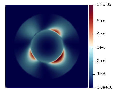
(b) $\hat{\mathcal{E}}_{u_{np}-a_{p}}$

Figure 32: Gresho Vortex: Entropy production fields at $t=0$ for the ES Turkel flux $M_{r}=3\times 10^{-2}$.

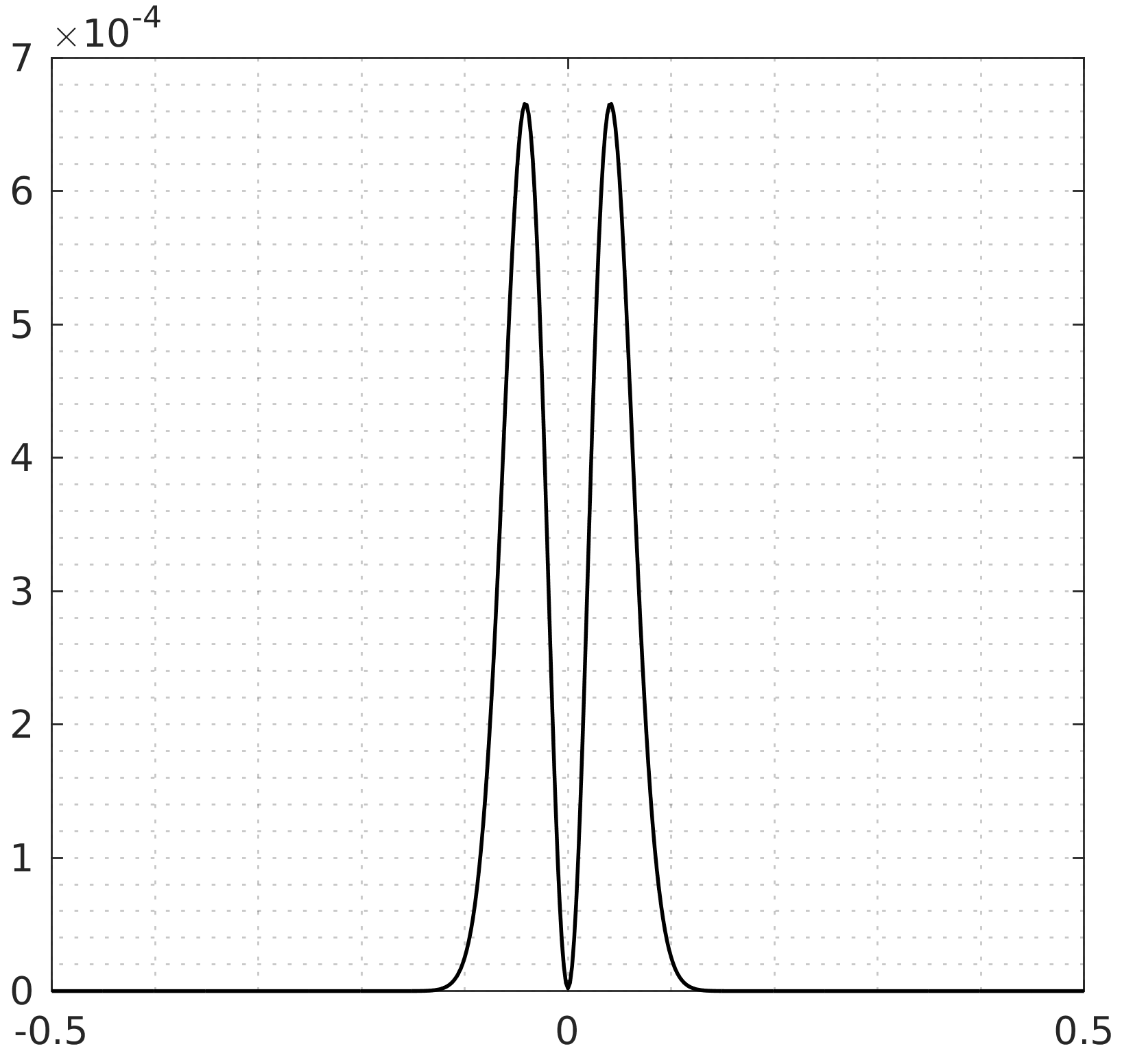
(a) $\hat{\mathcal{E}}_{u_{np}+a_{p}}$

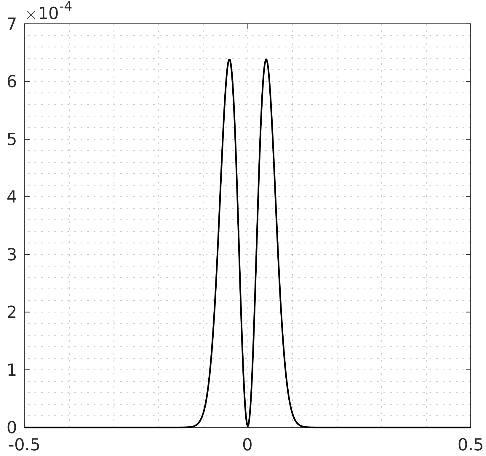
(b) $\hat{\mathcal{E}}_{u_{np}-a_{p}}$

Figure 33: Sound wave: Entropy production fields at $t=0$ for the ES Turkel flux $M_{r}=10^{-2}$.

Figures 32(a)-(b) show the modified acoustic entropy production fields for the Gresho vortex at $t=0$. The two fields are of the same magnitude and they appear to be in some sort of symmetry. Figures 14(a)-(c)-(e) show that the total acoustic entropy production fields are of the same order as those associated with the shear waves over time.
For the sound wave, the initial entropy production fields are shown in figures 33(a)-(b). The preconditioning leads to modified acoustic eigenvectors which can no longer be tied to right-moving and left-moving moving waves. The flow consists of a right-moving acoustic wave, yet we see that both entropy production fields $\mathcal{E}_{u_{np}\pm a_{p}}$ are active. Figures 14(b)-(d)-(f) show the overwhelming domination of both acoustic entropy production fields.

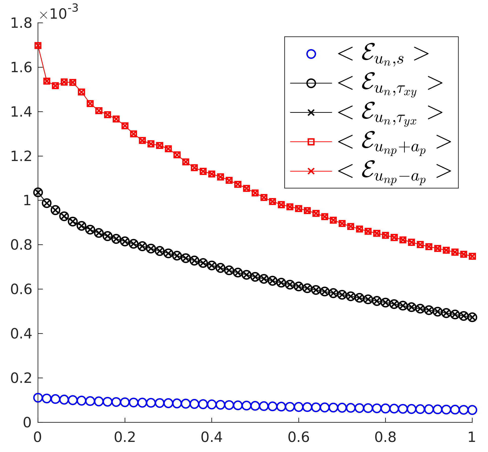
(a) Gresho Vortex - $M_{r}=3\times 10^{-1}$

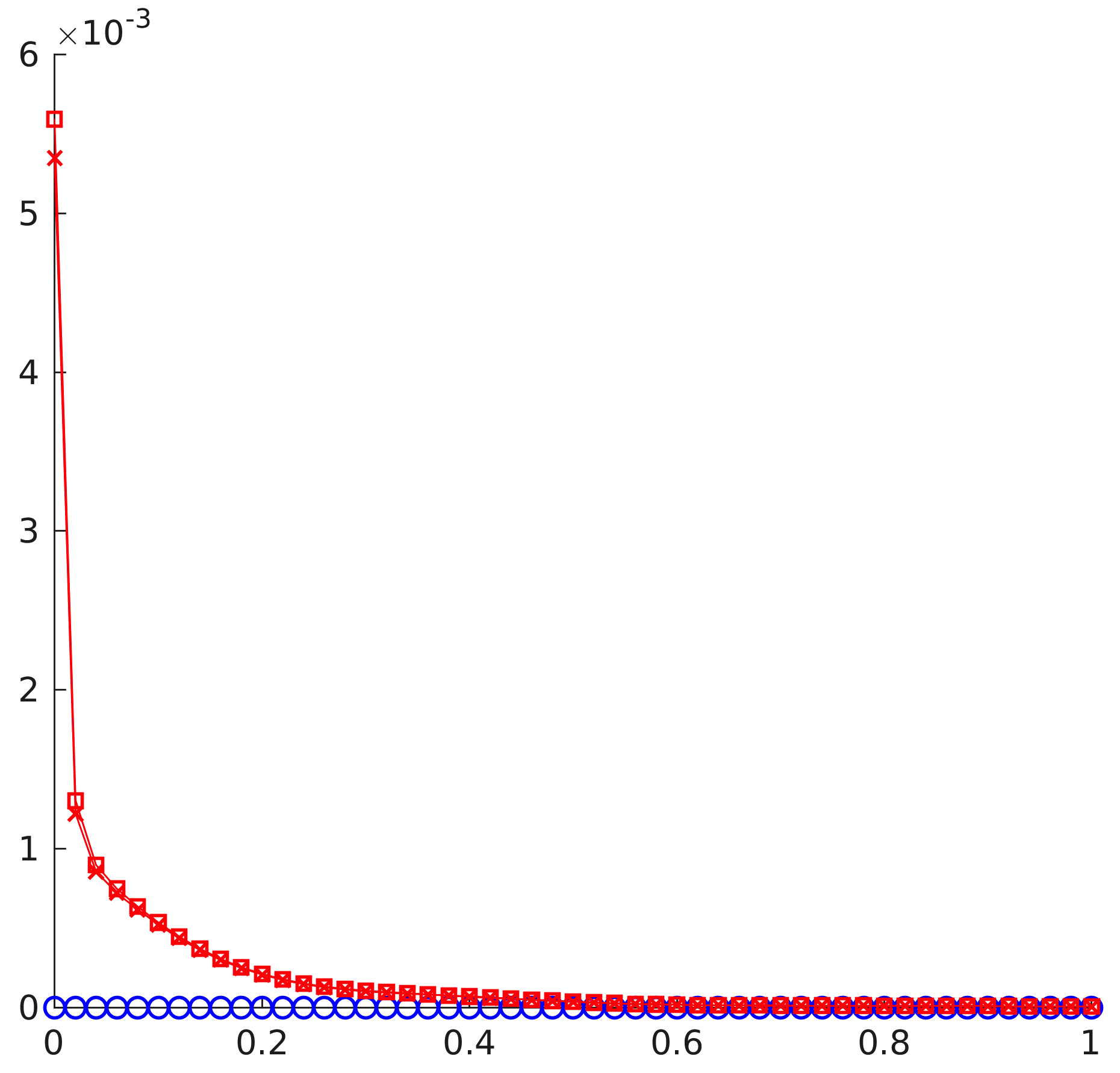
(b) Sound Wave - $M_{r}=10^{-2}$

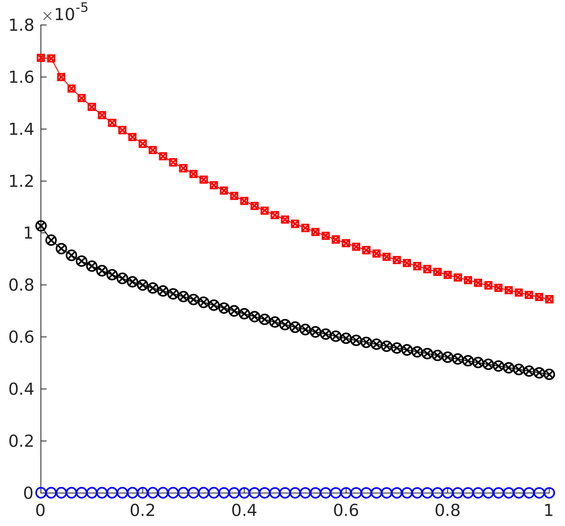
(c) Gresho Vortex - $M_{r}=3\times 10^{-2}$

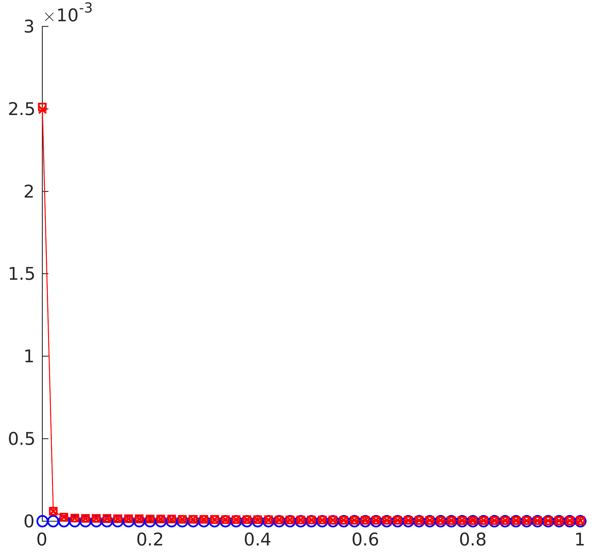
(d) Sound Wave - $M_{r}=10^{-3}$

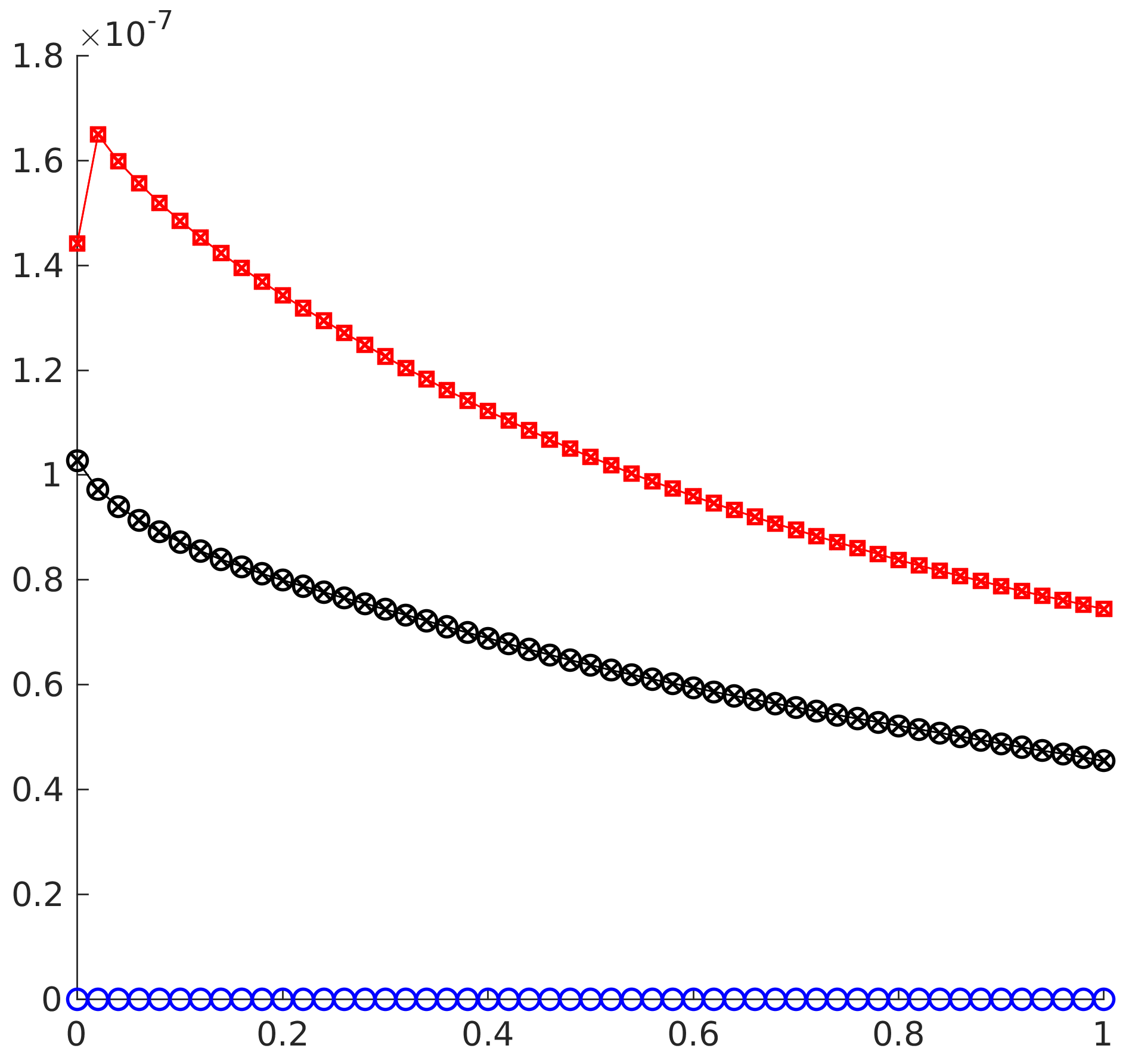
(e) Gresho Vortex - $M_{r}=3\times 10^{-3}$

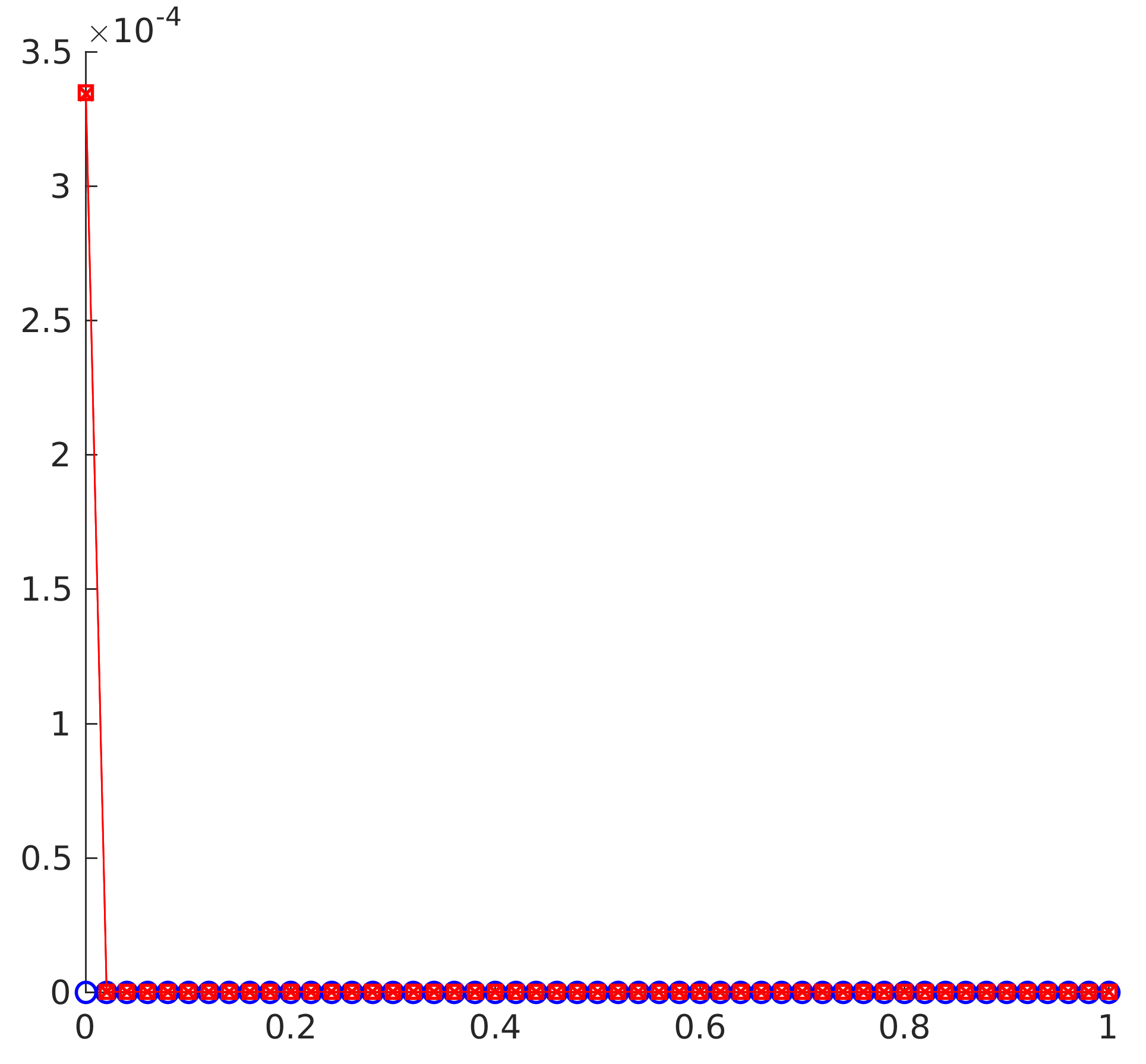
(f) Sound Wave - $M_{r}=10^{-4}$

Figure 14: Integral of each entropy production field with time at different Mach numbers for the ES Turkel flux on the Gresho Vortex (left) and the sound wave (right).

For Miczek’s matrix, we do not benefit from the eigenscaling theorem, but we do know that $T_{p}^{2}$ is positive definite. We have $R_{p}=[\mathbf{r}_{u_{n},1},\ \mathbf{r}_{u_{n},2},\ \mathbf{r}_{u_{n},3},\ \mathbf{r}_{u_{n}+a_{p}},\ \mathbf{r}_{u_{n}-a_{p}}]$ with:

$$\mathbf{r}_{u_{n}+a_{p}}=\sqrt{\frac{\rho}{\gamma}}\frac{1}{(p^{2}+1)(K_{1}-K_{2})}\begin{bmatrix}(K_{1}-p)\\ u(K_{1}-p)+(a/M_{r})n_{1}(K_{1}p+1)\\ v(K_{1}-p)+(a/M_{r})n_{2}(K_{1}p+1)\\ w(K_{1}-p)+(a/M_{r})n_{3}(K_{1}p+1)\\ h^{t}(K_{1}-p)+u_{n}(aM_{r})(K_{1}p+1)\end{bmatrix},$$

$$\mathbf{r}_{u_{n}-a_{p}}=\sqrt{\frac{\rho}{\gamma}}\frac{1}{(p^{2}+1)(K_{1}-K_{2})}\begin{bmatrix}(K_{2}-p)\\ u(K_{2}-p)+(a/M_{r})n_{1}(K_{2}p+1)\\ v(K_{2}-p)+(a/M_{r})n_{2}(K_{2}p+1)\\ w(K_{2}-p)+(a/M_{r})n_{3}(K_{2}p+1)\\ h^{t}(K_{2}-p)+u_{n}(aM_{r})(K_{2}p+1)\end{bmatrix},$$

and:

$$T_{p}^{2}=\begin{bmatrix}1&0&0&0&0\\ 0&1&0&0&0\\ 0&0&1&0&0\\ 0&0&0&K_{2}^{2}+1&(K_{2}-K_{1})p-K_{1}K_{2}-1\\ 0&0&0&(K_{1}-K_{2})p-K_{1}K_{2}-1&K_{1}^{2}+1\end{bmatrix}.$$

$T_{p}^{2}$ is not diagonal, but $D_{P}$ can be further reduced by observing that in the subsonic regime, the last 2-by-2 bloc of $|\Lambda_{p}|T_{p}^{2}$ can be decomposed into symmetric and skew-symmetric parts as follows

$$\big{(}|\Lambda_{p}|T_{p}^{2}\big{)}_{(4:5,4:5)}\ =\ \begin{bmatrix}|u_{n}+a_{p}|(K_{2}^{2}+1)&0\\ 0&|u_{n}-a_{p}|(K_{1}^{2}+1)\end{bmatrix}+\begin{bmatrix}0&-\delta_{p}\\ \delta_{p}&0\end{bmatrix},$$

$$\delta_{p}=2p(p^{2}+1)(a^{2}-M_{r}^{2}u_{n}^{2})/(M_{r}(a-M_{r}pu_{n})).$$

Instead of a symmetric form, we now have $D_{P}=R_{p}(|\Lambda_{p}|\overline{T}^{2}_{p}+\Delta_{p})R_{p}^{T}$ with:

$$\overline{T}^{2}_{p}=diag([1,\ 1,\ 1,\ K_{2}^{2}+1,\ K_{1}^{2}+1]),\ \Delta_{p}=\begin{bmatrix}0&0&0&0&0\\ 0&0&0&0&0\\ 0&0&0&0&0\\ 0&0&0&0&-\delta_{p}\\ 0&0&0&\delta_{p}&0\end{bmatrix}.$$

Since $\overline{T}^{2}_{p}$ is diagonal positive and $\Delta_{p}$ is skew-symmetric, it follows that $D_{P}$ is positive definite for the Miczek flux-preconditioner (hence the compatibility with entropy-stability). The EPB for Miczek’s flux is more subtle than for Turkel’s or Roe’s because of the skew symmetric matrix $\Delta_{p}$. We could ignore $\Delta_{p}$ in the EPB, since it does not contribute to $\mathcal{E}_{p}$. However, it turns out that this matrix plays a key role in the anomalies observed in the previous section.
Let $D^{A}_{P}[\mathbf{v}]$ denote the acoustic part of Miczek’s dissipation operator $R_{p}(\Lambda_{p}\overline{T}_{p}^{2}+\Delta_{p})R_{p}^{T}[\mathbf{v}]$. We have:

$$D^{A}_{P}[\mathbf{v}]=\begin{bmatrix}\mathbf{r}_{u_{n}+a_{p}}&\mathbf{r}_{u_{n}-a_{p}}\end{bmatrix}\begin{bmatrix}|u_{n}+a_{p}|(1+K_{2}^{2})&-\delta_{p}\\ \delta_{p}&|u_{n}-a_{p}|(1+K_{1}^{2})\end{bmatrix}\begin{bmatrix}\mu_{u_{n}+a_{p}}\\ \mu_{u_{n}-a_{p}}\end{bmatrix},$$ (88)

where $\mu_{u_{n}\pm a_{p}}=\ \mathbf{r}_{u_{n}\pm a_{p}}^{T}[\mathbf{v}]$ is given by:

$$\mu_{u_{n}+a_{p}}=\sqrt{\frac{\rho}{\gamma}}\frac{1}{(p^{2}+1)(K_{1}-K_{2})}\bigg{(}(K_{1}-p)\bigg{(}\mu_{0}-h\bigg{[}\frac{\rho}{p}\bigg{]}\bigg{)}+aM_{r}(K_{1}p+1)\overline{\bigg{(}\frac{\rho}{p}\bigg{)}}[u_{n}]\bigg{)},$$

$$\mu_{u_{n}-a_{p}}=\sqrt{\frac{\rho}{\gamma}}\frac{1}{(p^{2}+1)(K_{1}-K_{2})}\bigg{(}(K_{2}-p)\bigg{(}\mu_{0}-h\bigg{[}\frac{\rho}{p}\bigg{]}\bigg{)}+aM_{r}(K_{2}p+1)\overline{\bigg{(}\frac{\rho}{p}\bigg{)}}[u_{n}]\bigg{)}.$$

Expanding (88), we have:

$$D^{A}_{P}[\mathbf{v}]=\mathbf{r}_{u_{n}+a_{p}}\bigg{(}\mu_{u_{n}+a_{p}}|u_{n}+a_{p}|(1+K_{2}^{2})-\delta_{p}\mu_{u_{n}-a_{p}}\bigg{)}+\mathbf{r}_{u_{n}-a_{p}}\bigg{(}\mu_{u_{n}-a_{p}}|u_{n}-a_{p}|(1+K_{1}^{2})+\delta_{p}\mu_{u_{n}+a_{p}}\bigg{)}.$$ (89)

Multiplying on the left by $[\mathbf{v}]^{T}$ gives an acoustic entropy production field:

$$[\mathbf{v}]^{T}D^{A}_{P}[\mathbf{v}]=\mathcal{E}_{u_{n}+a_{p}}+\mathcal{E}_{u_{n}-a_{p}},$$ (90)

where the fields $\mathcal{E}_{u_{n}\pm a_{p}}$ break down into contributions $\{\mathcal{E}^{S}_{u_{n}\pm a_{p}},\ \mp\Delta\mathcal{E}^{p}\}$ from the symmetric and skew-symmetric parts of the dissipation operator:

$$\mathcal{E}_{u_{n}+a_{p}}=\mathcal{E}_{u_{n}+a_{p}}^{S}-\Delta\mathcal{E}_{p},\ \mathcal{E}_{u_{n}-a_{p}}=\mathcal{E}_{u_{n}-a_{p}}^{S}+\Delta\mathcal{E}_{p},$$ (91)

$$\mathcal{E}_{u_{n}+a_{p}}^{S}=\mu_{u_{n}+a_{p}}^{2}|u_{n}+a_{p}|(1+K_{2}^{2}),\ \mathcal{E}_{u_{n}-a_{p}}^{S}=\mu_{u_{n}-a_{p}}^{2}|u_{n}-a_{p}|(1+K_{1}^{2}),$$ (92)

$$\Delta\mathcal{E}_{p}=\delta_{p}\mu_{u_{n}+a_{p}}\mu_{u_{n}-a_{p}}.$$ (93)

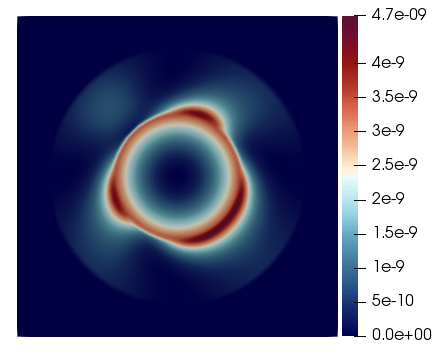
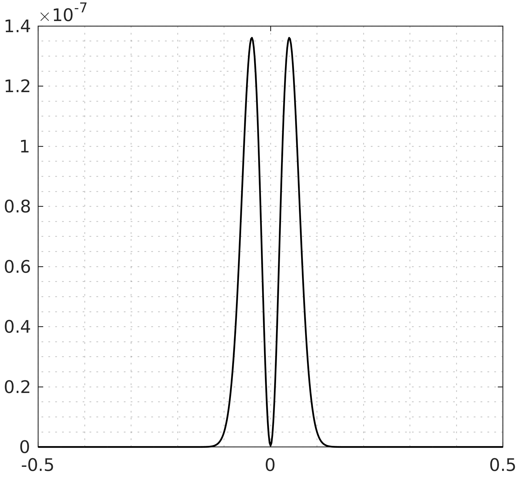
(d) $\hat{\mathcal{E}}^{S}_{u_{np}-a_{p}}$

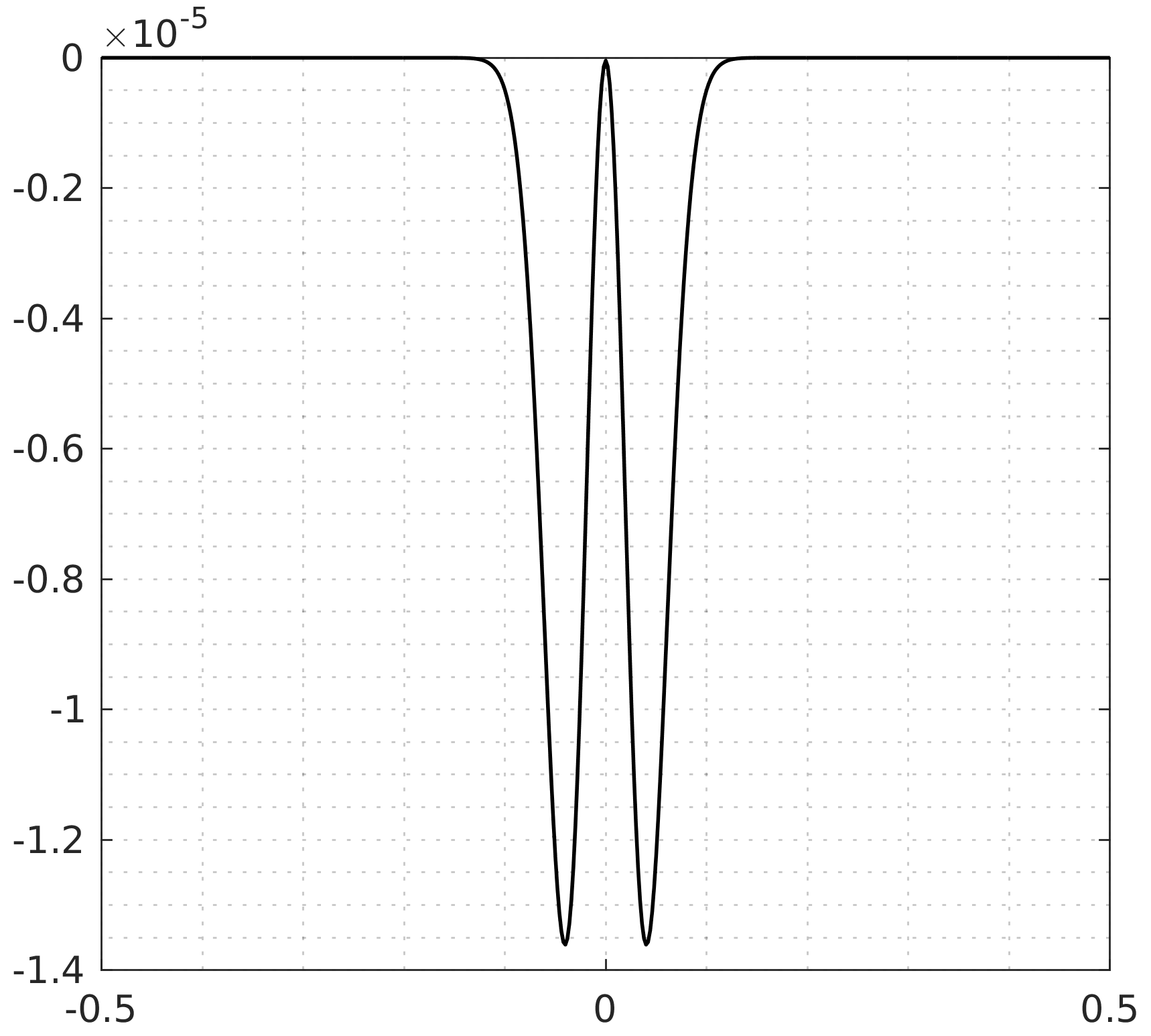
(e) $\Delta\hat{\mathcal{E}}_{p}$

Figure 34: Gresho Vortex: Entropy production fields at $t=0$ for the ES Miczek flux $M_{r}=3\times 10^{-2}$.

$\mathcal{E}_{u_{n}+a_{p}}$ and $\mathcal{E}_{u_{n}-a_{p}}$ are no longer positive in principle but their addition is always positive. Equations (89) and (91) suggest that while $\Delta_{p}$ does not change the discrete entropy production produced at an interface, it effects how this amount is distributed locally among acoustic modes.
Figures 34(a)-(b) show the modified acoustic entropy production fields for the Gresho vortex at $t=0$. They resemble those of the ES Turkel flux. Figures 34(c)-(e) show the contributions of the symmetric and skew-symmetric terms. The skew-symmetric component is not negligible. Figures 15(a)-(c) show that the total acoustic entropy production fields are of the same order as those associated with the shear waves over time. We also see that the total contribution $\langle\Delta\mathcal{E}_{p}\rangle$ from the skew-symmetric matrix evolves in time like a damped oscillator, with a characteristic time that decreases with the Mach number. This suggests that the spurious transient causing the phase errors we observed earlier has something to do with the skew-symmetric matrix. A simple way to confirm this is to multiply the skew-symmetric term by a factor and see how it impacts the solution. This is illustrated in figures 16(a)-(b). Taking out the skew-symmetric indeed removes the transient and phase errors. Making the skew-symmetric term stronger amplifies them. What’s more, figure 17 shows that the skew-symmetric term does not have a visible impact on the ability of the scheme to conserve the kinetic energy of the system.
For the sound wave, the initial entropy production fields are showed in figures 35(a)-(e). The contribution from the skew-symmetric part is two orders of magnitude bigger than the contribution from the symmetric part. This is why, for visibility, we show the integrated entropy production fields in two parts (figure 18). While the perturbations we observed in figure 8 appear in the symmetric parts $\mathcal{E}_{u_{n}\pm a_{p}}^{S}$ of the acoustic entropy production fields, it turns out from figures 19(a)-(b) that it is the skew-symmetric term again that is causing the appearance of a spurious left-moving acoustic wave. These observations lead us to the following statement:

Conjecture: The skew-symmetric matrix $$\Delta_{p}$$ in the Miczek ES flux causes entropy transfers among acoustic waves.

We examine this claim in more detail in section 7.

(a) $M_{r}=3\times 10^{-1}$

(b) $M_{r}=3\times 10^{-2}$

(c) $M_{r}=3\times 10^{-3}$

Figure 15: Gresho Vortex: Integral of each entropy production field with time at different Mach numbers for the ES Miczek flux.

(a) $t=1$

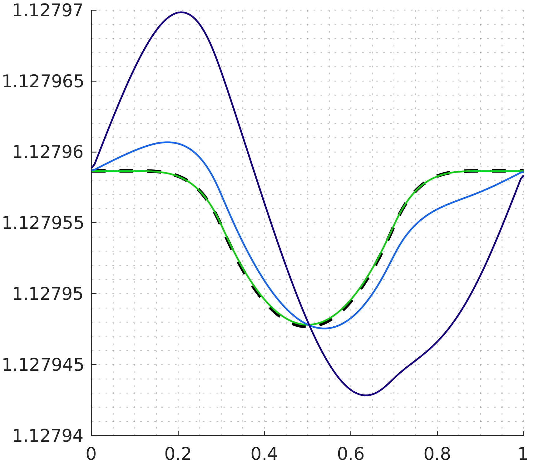
(b) $t=0.04$

Figure 16: Gresho Vortex: Pressure field at $M_{r}=3\times 10^{-3}$ for the Miczek flux when the skew-symmetric term is multiplied by a factor. The phase errors observed in figures 4 and 5 disappear if the skew-symmetric term is removed, and amplified if the skew-symmetric term is made bigger.

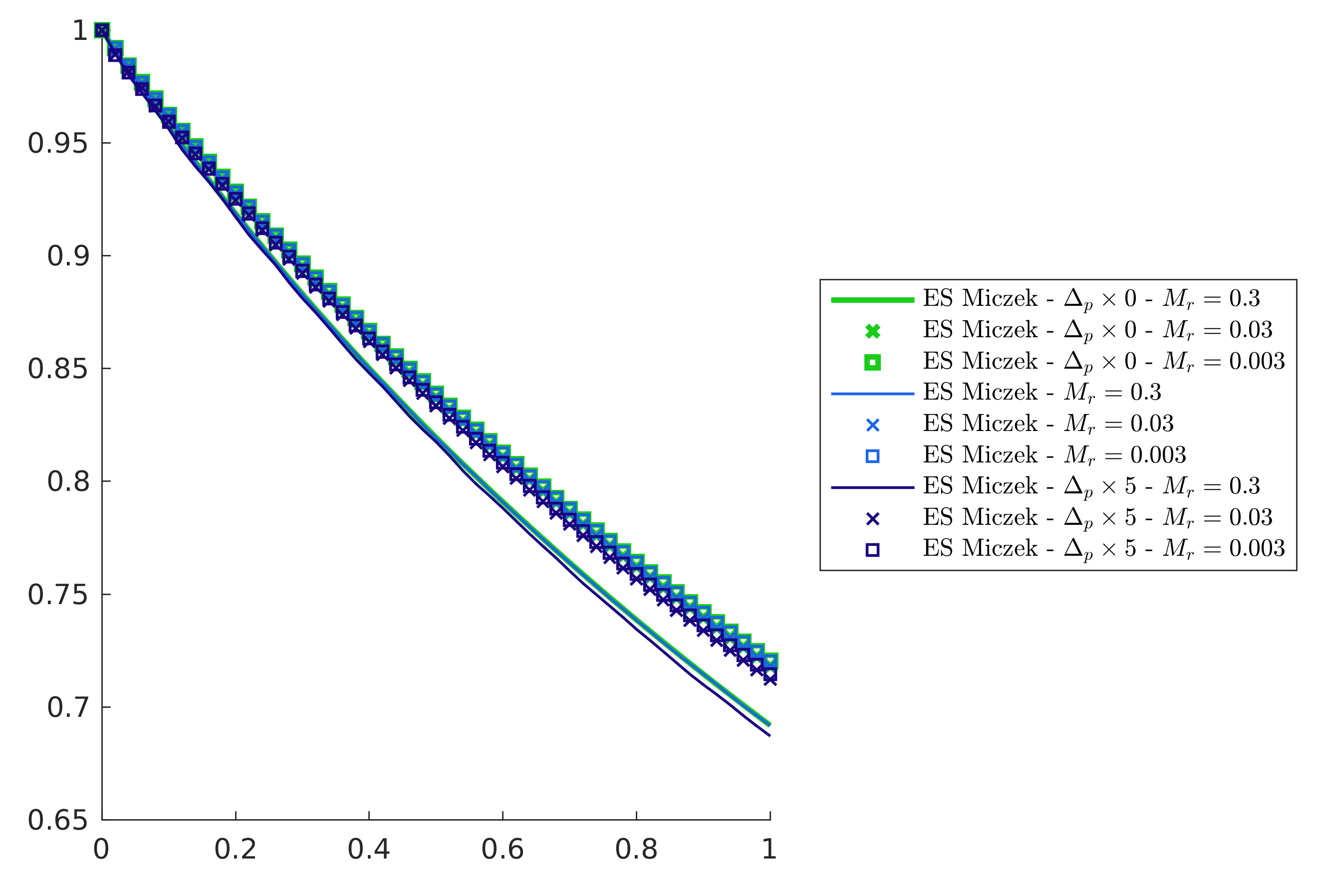
Figure 17: Gresho vortex: Total kinetic energy over time. The skew-symmetric matrix does not strongly impact the ability of the scheme to preserve the kinetic energy.

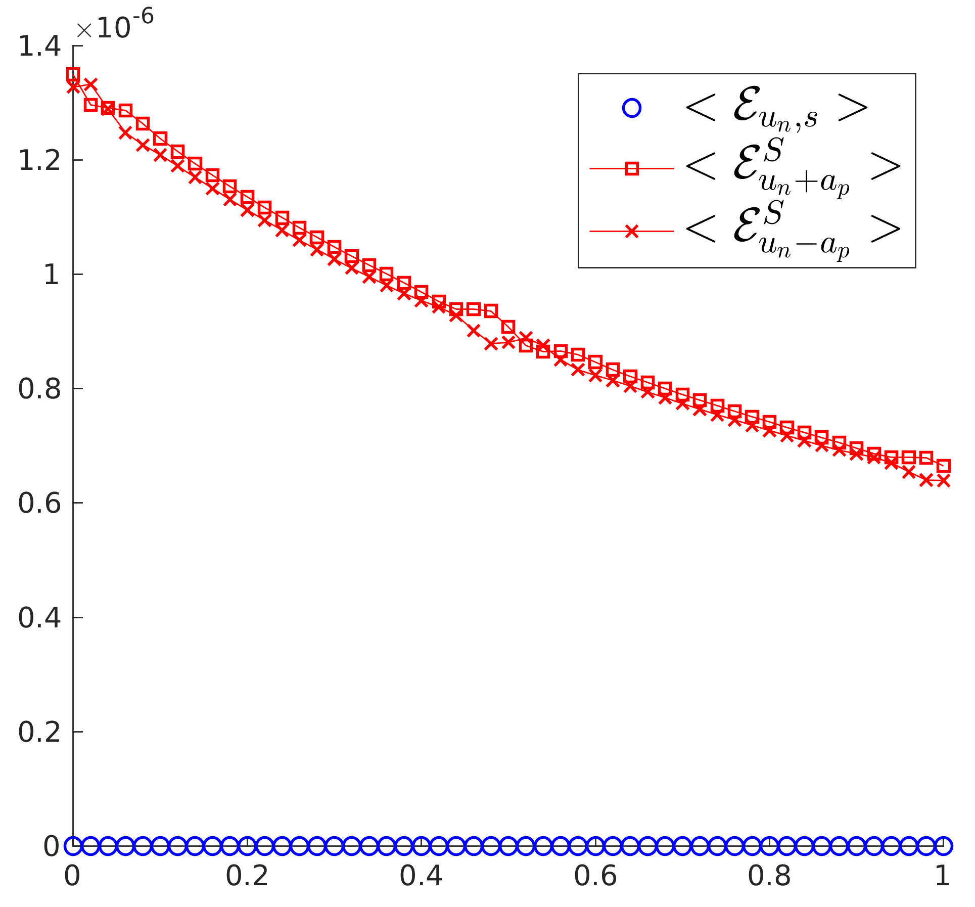
(a) Without $\Delta_{p}$

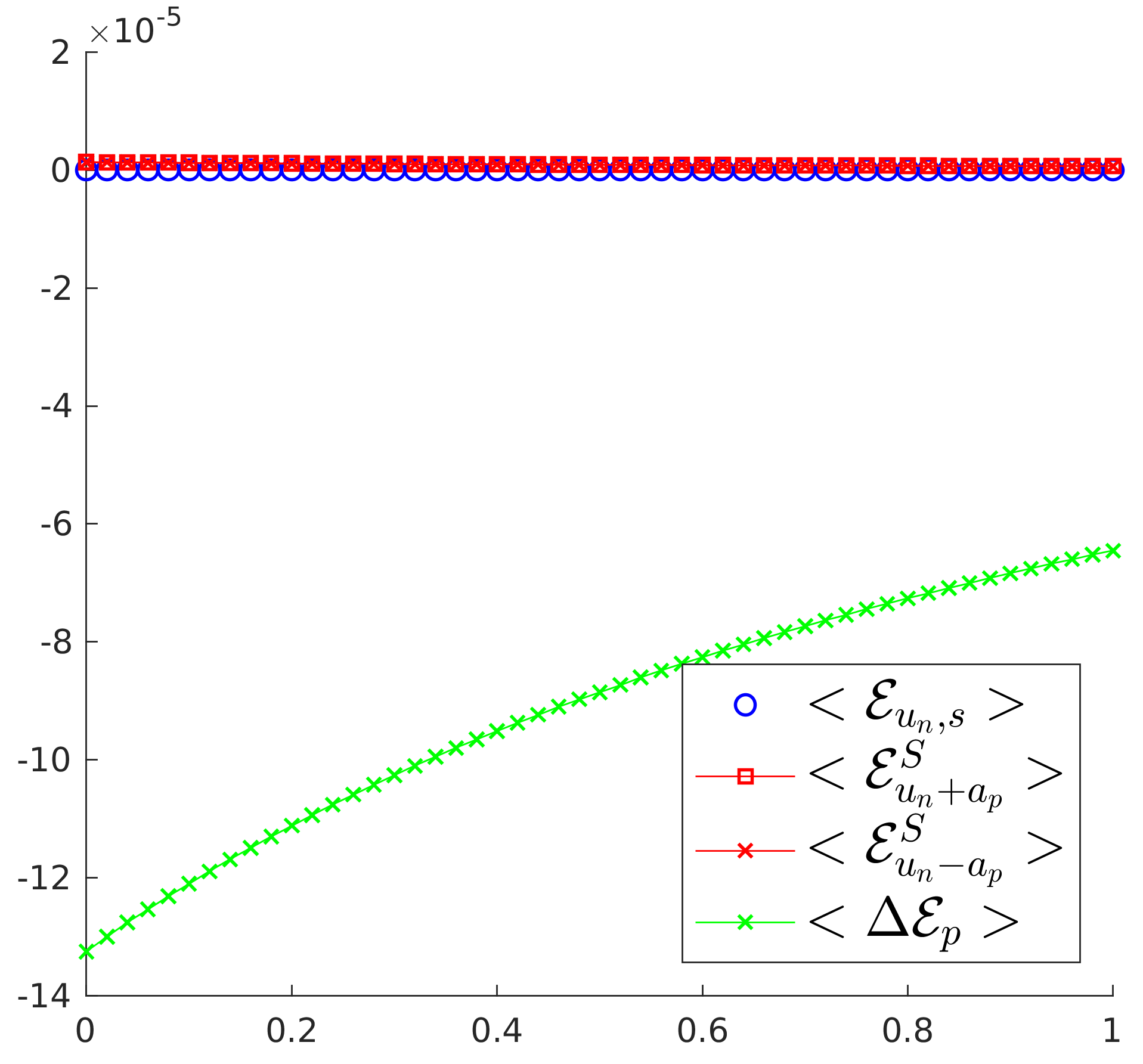
(b) With $\Delta_{p}$

Figure 18: Sound wave: Integral of entropy production fields for $M_{r}=10^{-2}$ (same trends at lower $M_{r}$ values) for the ES Miczek flux, omitting the contribution of the skew-symmetric matrix (left) and including it (right).

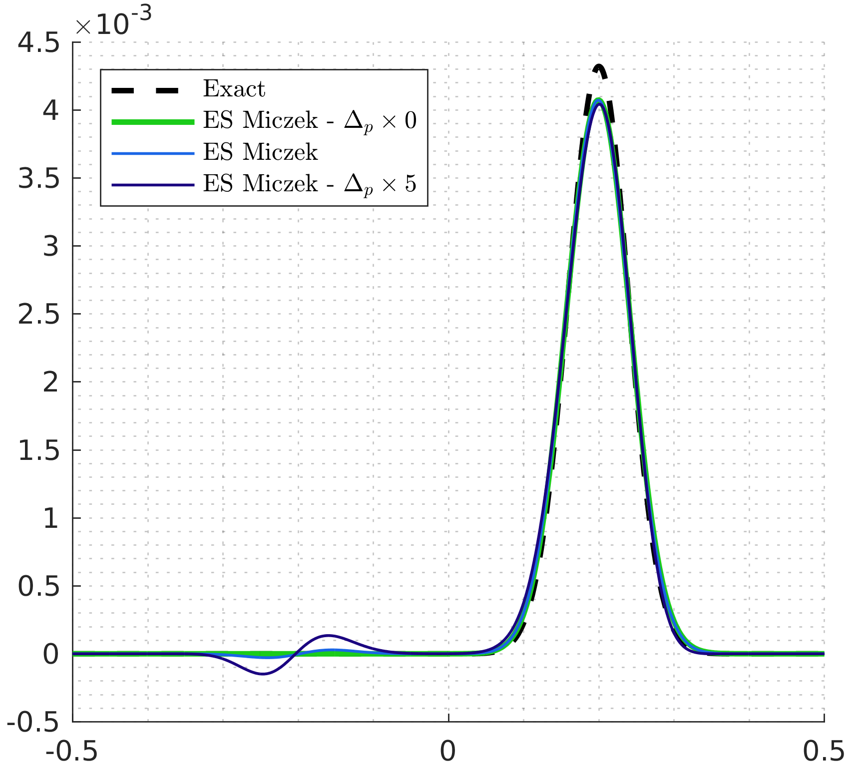
(a) $t=0.03$

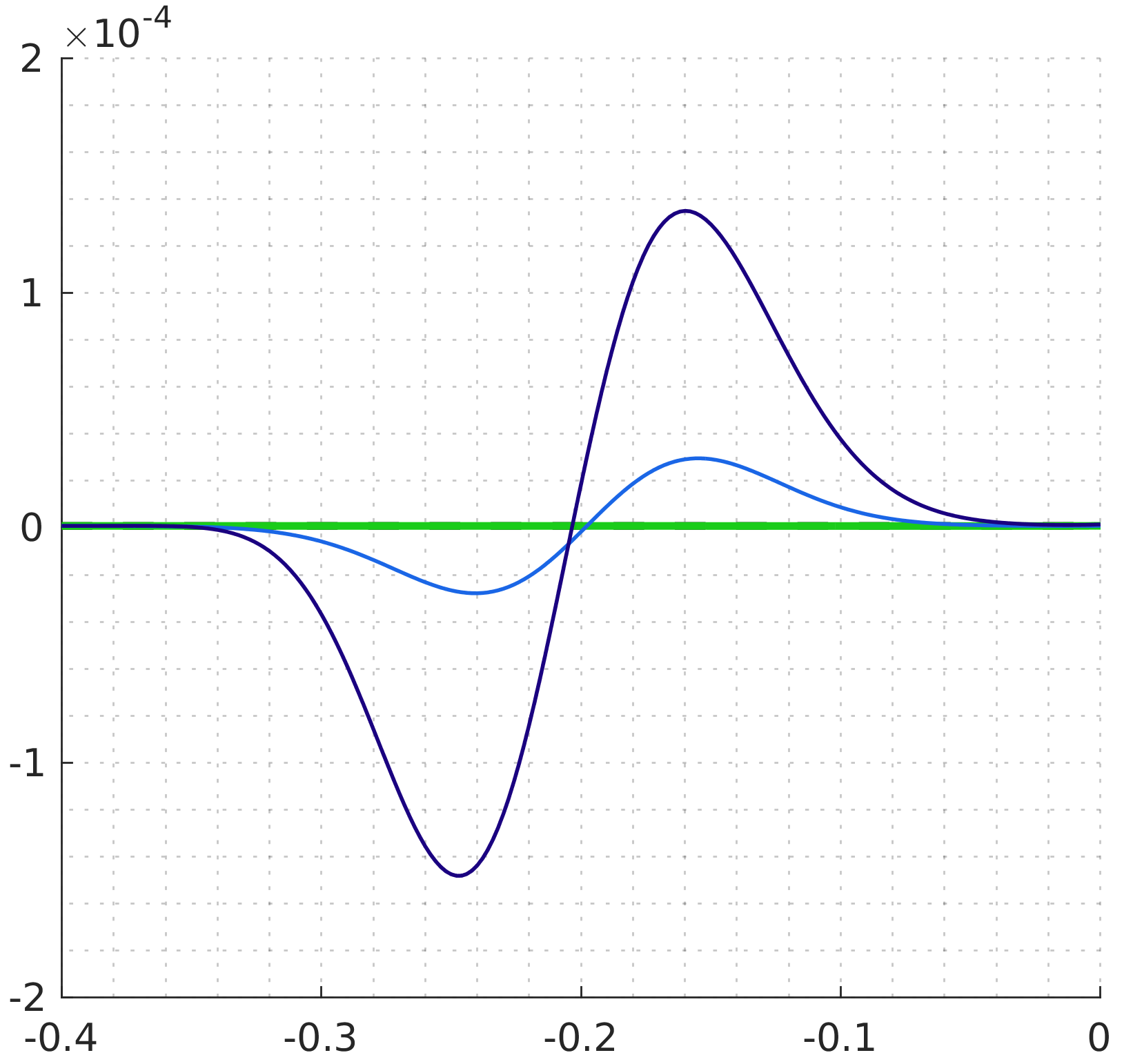
(b) $t=0.03$, zoomed

Figure 19: Sound wave: Pressure snapshots showing that the spurious left-moving acoustic wave is due to the skew-symmetric term in the ES Miczek flux. $M_{r}=10^{-2}$

6.2 The Discrete Low-Mach Regime Revisited

Using the analytical expressions we just derived, we can now determine how the entropy produced by each ES flux scales with respect to $M_{r}$ and establish whether (E.1) and (E.2) are satisfied. This effort, similar in spirit to the analysis of Guillard & Viozat Guillard1 , Guillard & Nkonga Guillard2 and Bruel et al. Bruel , provides an explanation to (S.1), (S.2) and (S.3) in terms of entropy production.
To verify the scaling analysis, we computed, for each ES flux, the integrated (79) entropy production fields at $t=0$ for the Gresho vortex and the sound wave at different reference Mach numbers. The scalings are shown in figures 20, 21 and 22.

Incompressible limit. For the Gresho vortex, density is constant, pressure and velocity variations are of order $M_{r}^{2}$ and $1$, respectively. At the discrete level, this translates into:

$$[\rho]=0,[p]=\mathcal{O}(M_{r}^{2}),\ [u]=\mathcal{O}(1),[v]=\mathcal{O}(1)\ \implies\\ \ \ \ [s]=\mathcal{O}(M_{r}^{2}),\ \bigg{[}\frac{\rho k}{p}\bigg{]}=\mathcal{O}(1),\ \bigg{[}\frac{\rho u}{p}\bigg{]}=\mathcal{O}(1),\ \bigg{[}\frac{\rho v}{p}\bigg{]}=\mathcal{O}(1),\ \bigg{[}\frac{\rho}{p}\bigg{]}=\mathcal{O}(M_{r}^{2}).$$ (94)

For the classic ES upwind dissipation, this gives:

$$\mu_{0}=\mathcal{O}(M_{r}^{2})\ \ \mbox{and}\ \ \mu_{s1}=\mu_{s2}=0,\ \mu_{s3}=\mathcal{O}(1)\ \implies \ \mathcal{E}_{u_{n},s}=\mathcal{O}(M_{r}^{4}),\ \mathcal{E}_{u_{n},\tau}=\mathcal{O}(M_{r}^{2}).$$ (95)

$$\mu_{u_{n}\pm a}=\mathcal{O}(M_{r})\ \implies \ \mathcal{E}_{u_{n}\pm a}=\mathcal{O}(M_{r}).$$ (96)

This implies that the overall discrete entropy production scales as $M_{r}$, that is one order of magnitude above what is expected. This explains the accuracy degradation observed.
With the flux-preconditioner of Turkel, we have $p=\mathcal{O}(M_{r})$, $a_{p},u_{np}=\mathcal{O}(1)$ and $K_{1},K_{2},K_{1}-K_{2}=\mathcal{O}(M_{r})$, therefore:

$$\mu_{u_{np}\pm a_{p}}=\mathcal{O}(1)\implies\mathcal{E}_{u_{np}\pm a_{p}}=\mathcal{O}(M_{r}^{2}).$$

That is the correct scaling. Hence the consistent behavior.
With the preconditioner of Miczek, we have $p=\mathcal{O}(1/M_{r})$, $a_{p}=\mathcal{O}(1/M_{r}^{2})$, $K_{2}=\mathcal{O}(M_{r})$ and $K_{1}=\mathcal{O}(1/M_{r})$ because its denominator writes:

$$M_{r}a_{p}-ap= \ M_{r}\sqrt{(p^{2}+1)a^{2}/M_{r}^{2}-p^{2}u_{n}^{2}}-ap$$

$$= \ ap\bigg{(}\sqrt{1+1/p^{2}-M_{r}^{2}u_{n}^{2}/a^{2}}-1\bigg{)}=\mathcal{O}(M_{r}).$$

Therefore:

$$\mu_{u_{n}+a_{p}}=\mathcal{O}(M_{r}^{2}),\ \mu_{u_{n}-a_{p}}=\mathcal{O}(M_{r}^{4})\ \implies\ \mathcal{E}_{u_{n}+a_{p}}^{S}=\mathcal{O}(M_{r}^{2}),\ \mathcal{E}_{u_{n}-a_{p}}^{S}=\mathcal{O}(M_{r}^{4}),$$

$$\delta_{p}=\mathcal{O}(1/M_{r}^{4}) \implies\Delta\mathcal{E}_{p}=\mathcal{O}(M_{r}^{2}).$$

Here again, the discrete entropy production has the correct scaling.

Acoustic limit. For the sound wave configuration, density, velocity and pressure gradients are of orders $M_{r}$, $1$ and $M_{r}$, respectively. The specific entropy is constant. At the discrete level, this translates into:

$$[\rho]=\mathcal{O}(M_{r}),[p]=\mathcal{O}(M_{r}),\ [u]=\mathcal{O}(1),\ [s]=0\implies\ \bigg{[}\frac{\rho k}{p}\bigg{]}=\mathcal{O}(1),\ \bigg{[}\frac{\rho u}{p}\bigg{]}=\mathcal{O}(1),\ \bigg{[}\frac{\rho}{p}\bigg{]}=\mathcal{O}(M_{r}).$$

For the classic ES upwind dissipation, this gives:

$$\mu_{0}=\mathcal{O}(M_{r}^{3})\ \ \mbox{and}\ \ \mu_{s1}=\mu_{s2}=\mu_{s3}=0\ \implies \ \mathcal{E}_{u_{n},s}=\mathcal{O}(M_{r}^{6}),\ \mathcal{E}_{u_{n},\tau}=0.$$ (97)

$$\mu_{u_{n}\pm a}=\mathcal{O}(M_{r})\ \implies \ \mathcal{E}_{u_{n}\pm a}=\mathcal{O}(M_{r}).$$ (98)

This implies that the overall discrete entropy production scales as $M_{r}$, in agreement with (E.2).
With Turkel’s preconditioner, we have:

$$\mu_{u_{np}\pm a_{p}}=\mathcal{O}(1/M_{r})\implies\mathcal{E}_{u_{np}\pm a_{p}}=\mathcal{O}(1),$$

meaning that entropy fluctuations will be one order of magnitude stronger than what is expected. This explains why sound waves are severely damped with this flux.
With Miczek’s preconditioner, we have:

$$\mu_{u_{n}+a_{p}}=\mathcal{O}(M_{r}^{2}),\ \mu_{u_{n}-a_{p}}=\mathcal{O}(M_{r}^{3})\ \implies\ \mathcal{E}_{u_{n}+a_{p}}^{S}=\mathcal{O}(M_{r}^{2}),\ \mathcal{E}_{u_{n}-a_{p}}^{S}=\mathcal{O}(M_{r}^{2}),\ \Delta\mathcal{E}_{p}=\mathcal{O}(M_{r})$$

The discrete entropy production is one order of magnitude weaker than what is expected. This can explain why the sound wave is less damped than with the ES Roe flux.

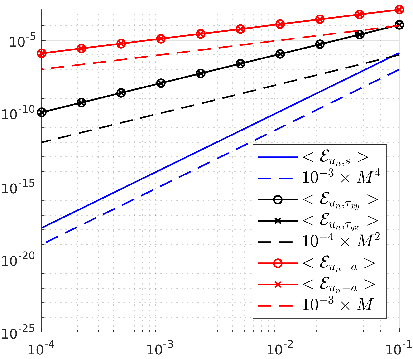
(a) Gresho Vortex

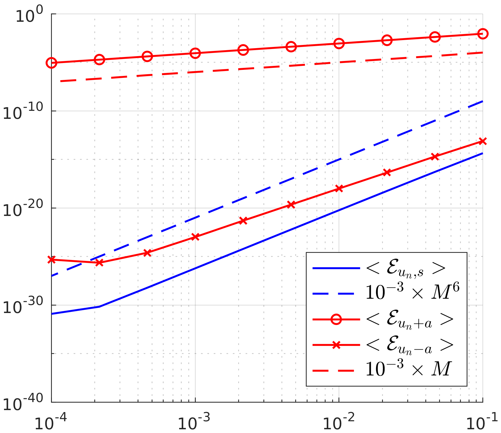
(b) Sound wave

Figure 20: Entropy production scalings - ES Roe flux

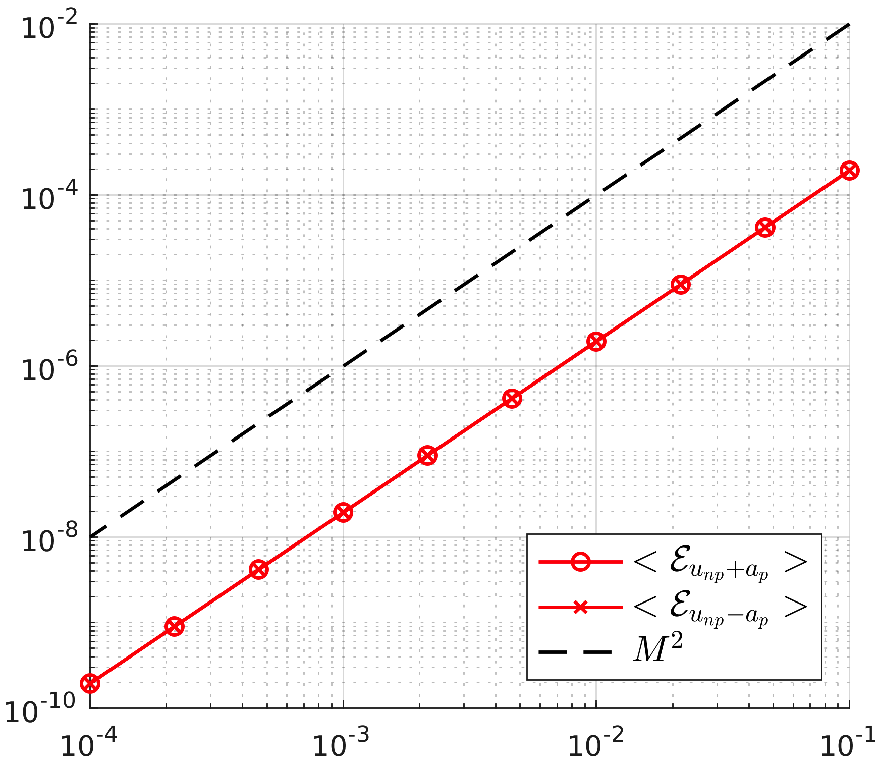
(a) Gresho Vortex

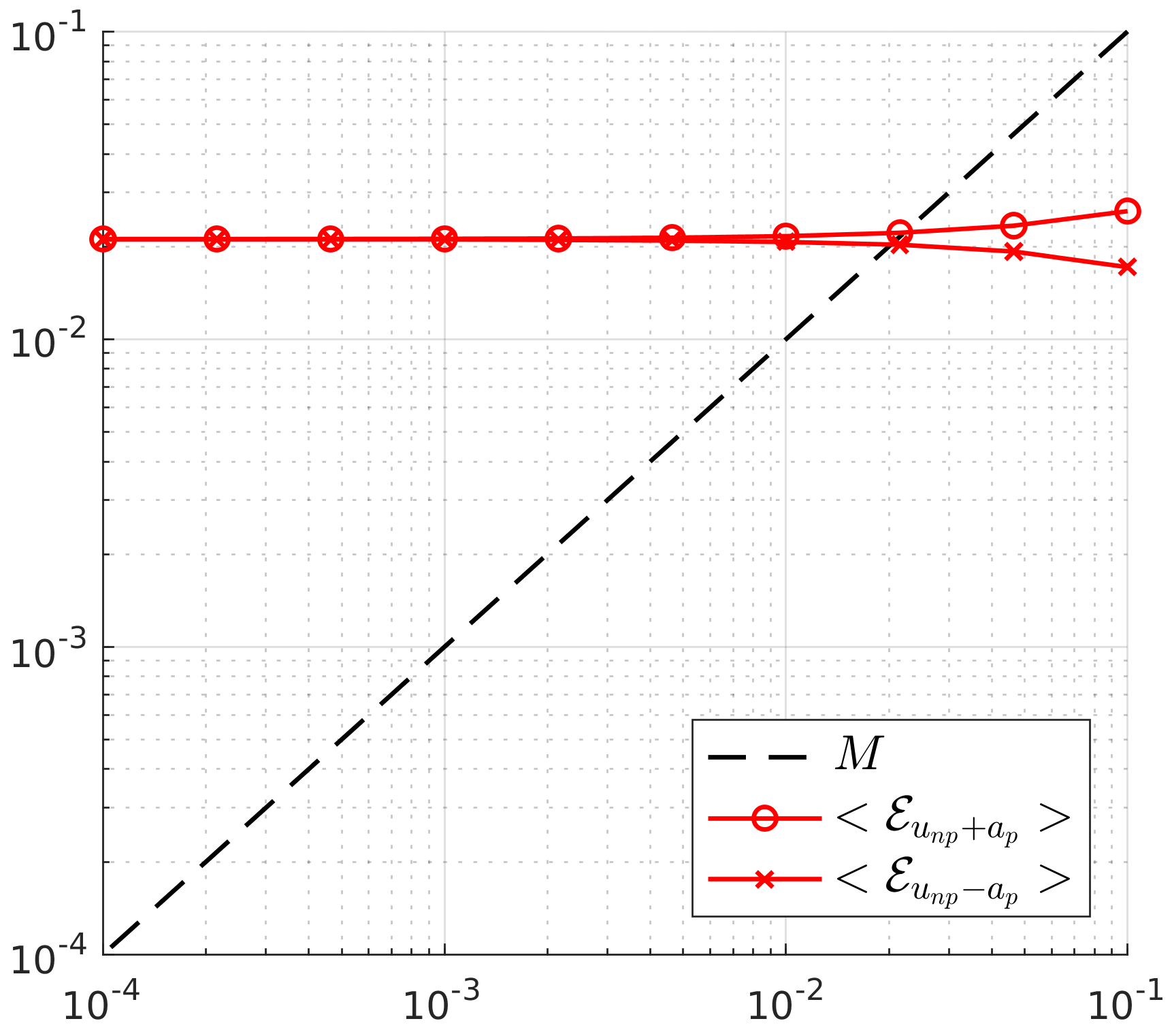
(b) Sound wave

Figure 21: Entropy production scalings - ES Turkel flux

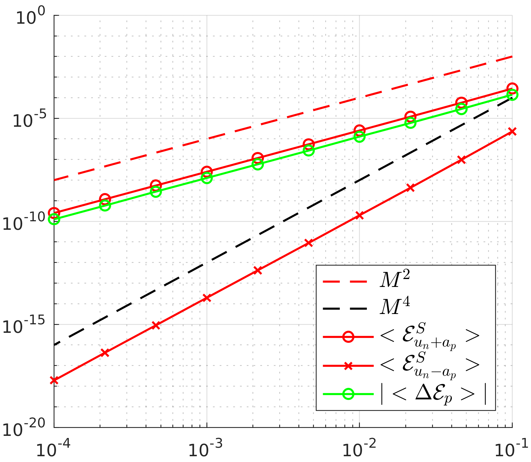
(a) Gresho Vortex

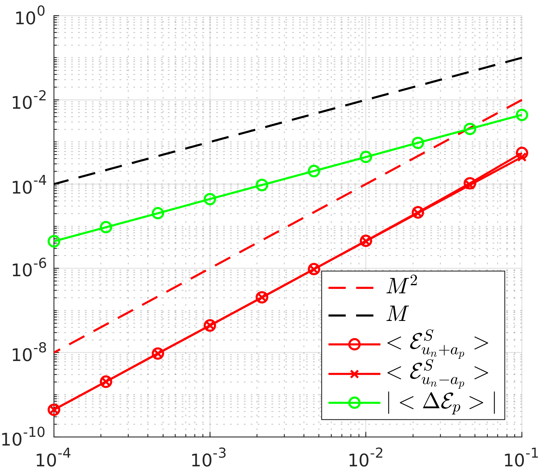
(b) Sound wave

Figure 22: Entropy production scalings - ES Miczek flux

6.3 Connections with other low-Mach fixes

Several alternatives to Flux-Preconditioning have been proposed, some of which are discussed in Guillard & Nkonga Guillard2 . They can be broken down into two categories. There are corrections based on the idea that the excessive dissipation in the low-Mach limit is due to the acoustic eigenvalues scaling as $\mathcal{O}(1/M_{r})$ and therefore becoming infinitely large. Li & Gu LiGu1 ; LiGu2 introduced an all-speed Roe-type scheme where the eigenvalues are modified as:

$$u_{n}\pm(a/M_{r})\ \rightarrow\ u_{n}\pm f(M_{r})(a/M_{r}),$$

and $f(M_{r})$ is a correction introduced so that $f(M_{r})(a/M_{r})$ is bounded in the low-Mach limit. This type of correction does not impede entropy-stability.
The second kind of correction Rieper ; Dellacherie ; Osswald consists in modifying the jump terms in the normal velocity $[u_{n}]$ (see also Thornber et al. Thornber1 ; Thornber2 ). By and large, they multiply $[u_{n}]$ by a correction term of order $M_{r}$. These fixes are motivated in part by the work of Birken & Meister Birken , who showed that the flux-preconditioner of Turkel enforce a more stringent (by a factor $M_{r}$) CFL condition (a similar result was proved by Barsukow et al. Barsukow for the flux-preconditioner of Miczek).
For the ES Roe flux, the acoustic part $D^{A}[\mathbf{v}]$ of the dissipation operator writes:

$$D^{A}[\mathbf{v}]=\begin{bmatrix}\mathbf{r}_{u_{n}+a}&\mathbf{r}_{u_{n}-a}\end{bmatrix}\begin{bmatrix}|u_{n}+(a/M_{r})|&0\\ 0&|u_{n}-(a/M_{r})|\end{bmatrix}\begin{bmatrix}\mu_{u_{n}+a}\\ \mu_{u_{n}-a}\end{bmatrix}$$ (99)

where

$$\mu_{u_{n}\pm a}=K_{a}\bigg{(}\mu_{0}-h\bigg{[}\frac{\rho}{p}\bigg{]}\pm M_{r}a\overline{\bigg{(}\frac{\rho}{p}\bigg{)}}[u_{n}]\bigg{)}.$$

Let $\tilde{\mu}_{u_{n}\pm a}$ be the wave strength obtained after applying the correction $[u_{n}]\rightarrow M_{r}[u_{n}]$:

$$\tilde{\mu}_{u_{n}\pm a}=K_{a}\bigg{(}\mu_{0}-h\bigg{[}\frac{\rho}{p}\bigg{]}\pm M_{r}^{2}a\overline{\bigg{(}\frac{\rho}{p}\bigg{)}}[u_{n}]\bigg{)}.$$

The resulting acoustic entropy production field $\tilde{\mathcal{E}}^{A}$ becomes:

$$\tilde{\mathcal{E}}^{A}=[\mathbf{v}]^{T}D^{A}[\mathbf{v}]=|u_{n}+(a/M_{r})|\mu_{u_{n}+a}\tilde{\mu}_{u_{n}+a}\ +\ |u_{n}-(a/M_{r})|\mu_{u_{n}-a}\tilde{\mu}_{u_{n}-a}.$$

It is not clear whether the resulting operator leads to an ES flux as the sign of $\tilde{\mathcal{E}}^{A}$ is not clear, but we have $\tilde{\mathcal{E}}^{A}=\mathcal{O}(M_{r}^{2})$ in the incompressible limit, in agreement with (E.1).

7 Discussion

7.1 The origin of the skew-symmetric term

Given that the Miczek flux-preconditioner was constructed so that $P^{-1}|PA|$ has the same scaling as $A$, the appearance of a skew-symmetric term in the scaled form of the Miczek ES dissipation operator could be explained by examining the acoustic entropy production field without upwinding, that is with $\Lambda$ instead of $|\Lambda|$. We have:

$$\mathcal{E}_{u_{n}+a}=\mu_{u_{n}+a}^{2}(u_{n}+(a/M_{r})),\ \mathcal{E}_{u_{n}-a}=\mu_{u_{n}-a}^{2}(u_{n}-(a/M_{r})).$$ (100)

If we assume $\mu_{u_{n}+a}^{2}\approx\mu_{u_{n}-a}^{2}\approx\mu_{u_{n}+a}\mu_{u_{n}-a}$, then we can write something similar to (91):

$$\mathcal{E}_{u_{n}+a}\approx\mathcal{E}^{S}_{u_{n}+a}+\Delta\mathcal{E}_{a},\ \mathcal{E}_{u_{n}-a}\approx\mathcal{E}^{S}_{u_{n}-a}-\Delta\mathcal{E}_{a},$$ (101)

where:

$$\mathcal{E}^{S}_{u_{n}+a}=\mu_{u_{n}+a}^{2}u_{n},\ \Delta\mathcal{E}_{a}=\mu_{u_{n}+a}\mu_{u_{n}-a}(a/M_{r}),\ \mathcal{E}^{S}_{u_{n}-a}=\mu_{u_{n}-a}^{2}u_{n}.$$

As a matter of course, the resulting dissipation operator is no longer guaranteed to be ES. The point is that the entropy production balance between acoustic fields described by equation (101) might be what the skew-symmetric matrix $\Delta_{p}$ of the ES Miczek flux tries to reproduce. Whether recovering this balance is key in ensuring a good low-Mach behavior is a different story. The numerical results (section 5) advise against it, at least at first-order.

7.2 A simple equivalent to the ES Miczek flux

Consider the dissipation operator $D_{P}=R(|\Lambda_{p}|+\Delta_{p})R^{T}$ where $R$ is the scaled eigenvector matrix of the ES Roe flux (Section 6.1.) and:

$$|\Lambda_{p}|=\begin{bmatrix}|u_{n}|&0&0&0&0\\ 0&|u_{n}|&0&0&0\\ 0&0&|u_{n}|&0&0\\ 0&0&0&f_{1}|u_{n}+(a/M_{r})|&0\\ 0&0&0&0&f_{2}|u_{n}-(a/M_{r})|\end{bmatrix},\ \Delta_{p}=g\begin{bmatrix}0&0&0&0&0\\ 0&0&0&0&0\\ 0&0&0&0&0\\ 0&0&0&0&+\delta_{p}\\ 0&0&0&-\delta_{p}&0\end{bmatrix},$$

and $f_{1},f_{2}$ and $g$ are functions of $M_{r}$. The eigenvectors $R$ are left untouched. Similarly to (91) and (101), we have:

$$\mathcal{E}_{u_{n}-a}=\mathcal{E}_{u_{n}-a}^{S}-g\Delta\mathcal{E}_{p},\ \mathcal{E}_{u_{n}+a}=\mathcal{E}_{u_{n}+a}^{S}+g\Delta\mathcal{E}_{p}$$

$$\mathcal{E}_{u_{n}-a}^{S}=\mu_{u_{n}-a}^{2}f_{2}|u_{n}-a|,\ \Delta\mathcal{E}_{p}=\delta_{p}\mu_{u_{n}-a}\mu_{u_{n}+a},\ \mathcal{E}_{u_{n}+a}^{S}=\mu^{2}_{u_{n}+a}f_{1}|u_{n}+a|).$$

This dissipation operator is ES as long as $f_{1},f_{2}\geq 0$, and we can emulate equation (101) by taking $f_{1}=|u_{n}|/|u_{n}+a/M_{r}|$, $f_{2}=|u_{n}|/|u_{n}-a/M_{r}|$, $g=1$ and $\delta_{p}=a/M_{r}$. This gives:

$$\mathcal{E}_{u_{n}-a}^{S}=\mu_{u_{n}-a}^{2}|u_{n}|,\ \Delta\mathcal{E}_{p}=\mu_{u_{n}-a}\mu_{u_{n}+a}(a/M_{r}),\ \mathcal{E}_{u_{n}+a}^{S}=\mu^{2}_{u_{n}+a}|u_{n}|.$$

In the incompressible and acoustic limits, we have:

$$\mathcal{E}_{u_{n}-a}^{S}=\mathcal{O}(M_{r}^{2}),\ \Delta\mathcal{E}_{p}=\mathcal{O}(M_{r}),\ \mathcal{E}_{u_{n}+a}^{S}=\mathcal{O}(M_{r}^{2}),$$

which meets the low-Mach requirements (E.1) and (E.2). This dissipation operator also meets Miczek’s requirement that the dissipation matrix should have exactly the same Mach number scalings as $A$. Remarkably, we have:

$$R_{\mathbf{z}}(|\Lambda_{p}|+\Delta_{p})R_{\mathbf{z}}^{-1}=\begin{bmatrix}|u_{n}|&-n_{x}a/M_{r}&-n_{y}a/M_{r}&-n_{z}a/M_{r}&0\\ n_{x}a/M_{r}&|u_{n}|&0&0&0\\ n_{y}a/M_{r}&0&|u_{n}|&0&0\\ n_{z}a/M_{r}&0&0&|u_{n}|&0\\ 0&0&0&0&|u_{n}|\end{bmatrix}.$$

To have this ”skewed” ES dissipation operator return to Roe’s as $M_{r}\rightarrow 1$, we can set $f_{1}=M_{r}+(1-M_{r})|u_{n}|/|u_{n}+(a/M_{r})|$, $f_{2}=M_{r}+(1-M_{r})|u_{n}|/|u_{n}-(a/M_{r})|$, and $g=1-M_{r}$ for instance. Numerical results (figures 23 and 24) show that this operator behaves just like the ES Miczek dissipation operator for both the Gresho vortex and the sound wave. The skewed ES dissipation operator (7.2) has not been introduced to compete with Miczek’s flux or any of the aforementioned schemes (we remind the reader that the best results were observed with an EC flux in space). We introduced it to assess our intuition that skew-symmetric dissipation operators change the way entropy is locally produced. The skewed dissipation operator can be easily shown to induce a $\mathcal{O}(M_{r}^{2})$ CFL condition, like the Turkel Birken and Miczek Barsukow dissipation operators (see appendix C in Gouasmi_Thesis ).

(a) $t=1$

(b) $t=0.04$

Figure 23: Gresho Vortex: Pressure field at $M_{r}=3\times 10^{-3}$ for the skewed ES flux when the skew-symmetric term is multiplied by different factors.

(a) $t=0.03$

(b) $t=0.03$, zoomed

Figure 24: Sound wave: Centerline pressure profiles with the skewed ES flux instead. $M_{r}=10^{-2}$.

7.3 Different ways of breaking down discrete entropy production

It is important to recognize that the EPB we introduced in section 6.1 is not unique. Consider a dissipation operator consisting of two linearly independent modes $R=[\mathbf{r_{1}},\ \mathbf{r_{2}}]$. We have:

$$R|\Lambda|R^{T}[\mathbf{v}]=|\lambda_{1}|\mu_{1}\mathbf{r_{1}}+|\lambda_{2}|\mu_{2}\mathbf{r_{2}}\ \implies\ \mathcal{E}=[\mathbf{v}]^{T}R|\Lambda|R^{T}[\mathbf{v}]=\mathcal{E}_{1}+\mathcal{E}_{2}.$$

Let $\overline{R}=\{\mathbf{\bar{r}_{1}},\ \mathbf{\bar{r}_{2}}\}$ be an alternative pair of linearly independent modes defined by the mapping:

$$\begin{cases}\mathbf{r_{1}}=l_{11}\mathbf{\bar{r}_{1}}+l_{12}\mathbf{\bar{r}_{2}},\\ \mathbf{r_{2}}=l_{21}\mathbf{\bar{r}_{1}}+l_{22}\mathbf{\bar{r}_{2}}.\end{cases}\ \implies\ \begin{cases}\mu_{1}=l_{11}\bar{\mu}_{1}+l_{12}\bar{\mu}_{2},\\ \mu_{2}=l_{21}\bar{\mu}_{1}+l_{22}\bar{\mu}_{2}.\end{cases}$$

Then the dissipation operator can be expressed in terms of these modes:

$$R|\Lambda|R^{T}[\mathbf{v}]=\big{(}L_{11}\bar{\mu}_{1}+L_{12}\bar{\mu}_{2}\big{)}\mathbf{\bar{r}_{1}}+\big{(}L_{22}\bar{\mu}_{2}+L_{21}\bar{\mu}_{1}\big{)}\mathbf{\bar{r}_{2}},$$

with:

$$L_{11}=(|\lambda_{1}|l_{11}^{2}+|\lambda_{2}|l_{21}^{2})>0,\ L_{22}=(|\lambda_{1}|l_{12}^{2}+|\lambda_{2}|l_{22}^{2})>0,\ L_{12}=L_{21}=(|\lambda_{1}|l_{11}l_{12}+|\lambda_{2}|l_{21}l_{22}).$$

This gives the EPB:

$$\mathcal{E}\ =\overline{\mathcal{E}}_{1}+\overline{\mathcal{E}}_{2},\ \overline{\mathcal{E}_{1}}=L_{11}\overline{\mu}_{1}^{2}+L_{12}\overline{\mu}_{1}\overline{\mu}_{2},\ \overline{\mathcal{E}_{2}}=L_{22}\overline{\mu}_{2}^{2}+L_{21}\overline{\mu}_{1}\overline{\mu}_{2}$$ (102)

Unlike the initial decomposition, each individual field $\overline{\mathcal{E}}_{i}$ is no longer guaranteed to be positive. This does not matter much given that the sign of $\mathcal{E}$ will not change. We also see that depending on the choice of modes, coupling terms within each field $\overline{\mathcal{E}}_{i}$ may appear. We can write:

$$\overline{\mathcal{E}}_{k}=\overline{\mathcal{E}}^{S}_{k}+\sum_{k^{\prime}\neq k}\overline{\mathcal{E}}_{kk^{\prime}},\ \overline{\mathcal{E}}^{S}_{k}=L_{kk}\bar{\mu}_{k}^{2},\ \overline{\mathcal{E}}_{kk^{\prime}}=L_{kk^{\prime}}\bar{\mu}_{k}\bar{\mu}_{k^{\prime}}.$$ (103)

Note that the coupling terms do not cancel each other, i.e. $\overline{\mathcal{E}}_{kk^{\prime}}+\overline{\mathcal{E}}_{k^{\prime}k}=0,\ k\neq k^{\prime}$. In fact, they are equal $\overline{\mathcal{E}}_{kk^{\prime}}=\overline{\mathcal{E}}_{k^{\prime}k}$.
If the dissipation operator has a skew-symmetric component:

$$R\Delta R^{T}[\mathbf{v}]=\delta(\mu_{2}\mathbf{r_{1}}-\mu_{1}\mathbf{r_{2}})\implies[\mathbf{v}]^{T}R\Delta R^{T}[\mathbf{v}]=\Delta\mathcal{E}-\Delta\mathcal{E}=0,\ \Delta\mathcal{E}=\delta\mu_{1}\mu_{2},$$

we can rewrite it in terms of $\{\mathbf{\bar{r}_{1}},\ \mathbf{\bar{r}_{2}}\}$ instead. Remarkably, we have:

$$R\Delta R^{T}[\mathbf{v}]\ =\ \delta(\mu_{2}\mathbf{r_{1}}-\mu_{1}\mathbf{r_{2}})\ =\ \delta(l_{11}l_{22}-l_{12}l_{21})\big{(}\bar{\mu}_{2}\mathbf{\bar{r}_{1}}-\bar{\mu}_{1}\mathbf{\bar{r}_{2}}\big{)}\ =\ \overline{\delta}\big{(}\bar{\mu}_{2}\mathbf{\bar{r}_{1}}-\bar{\mu}_{1}\mathbf{\bar{r}_{2}}\big{)}$$

The mapping is one-to-one hence $l_{11}l_{22}-l_{12}l_{21}\neq 0$. This shows that the skew-symmetric operator $R\Delta R^{T}[\mathbf{v}]$ (entropy transfer between modes $\{\mathbf{r_{1}},\ \mathbf{r_{2}}\}$) is equivalent to a skew-symmetric operator $\overline{R}\ \overline{\Delta}\ \overline{R}^{T}[\mathbf{v}]$ (entropy transfer between $\{\mathbf{\overline{r}_{1}},\ \mathbf{\overline{r}_{2}}\}$):

$$[\mathbf{v}]^{T}\overline{R}\ \overline{\Delta}\ \overline{R}^{T}[\mathbf{v}]=\overline{\Delta\mathcal{E}}-\overline{\Delta\mathcal{E}}=0,\ \overline{\Delta\mathcal{E}}=\overline{\delta}\overline{\mu}_{1}\overline{\mu}_{2}.$$

Using the above algebra, we can now introduce EPBs for the ES Turkel and ES Miczek fluxes in terms of the original acoustic eigenvectors instead of the modified ones. For Turkel’s flux-preconditioner, we map from $\{\mathbf{r_{1}},\ \mathbf{r_{2}}\}=\{\mathbf{r}_{u_{np}+a_{p}},\ \mathbf{r}_{u_{np}-a_{p}}\}$ to $\{\mathbf{\overline{r}_{1}},\ \mathbf{\overline{r}_{2}}\}=\{\mathbf{r}_{u_{n}+a},\ \mathbf{r}_{u_{n}-a}\}$ using:

$$\mathbf{r}_{u_{np}+a_{p}}=\frac{1}{\sqrt{2}p^{2}(K_{1}-K_{2})}\bigg{(}(K_{1}+p^{2})\mathbf{r}_{u_{n}+a}+(K_{1}-p^{2})\mathbf{r}_{u_{n}-a}\bigg{)},$$

$$\mathbf{r}_{u_{np}-a_{p}}=\frac{1}{\sqrt{2}p^{2}(K_{1}-K_{2})}\bigg{(}(K_{2}+p^{2})\mathbf{r}_{u_{n}+a}+(K_{2}-p^{2})\mathbf{r}_{u_{n}-a}\bigg{)}.$$

The new decomposition (102)-(103) (to contrast with (86)) writes:

$$\mathcal{E}_{p}\ =\ \big{(}\mathcal{E}^{S}_{u_{n}+a}+\mathcal{E}_{u_{n}+a,u_{n}-a}\big{)}+\big{(}\mathcal{E}^{S}_{u_{n}-a}+\mathcal{E}_{u_{n}-a,u_{n}+a}\big{)}.$$ (104)

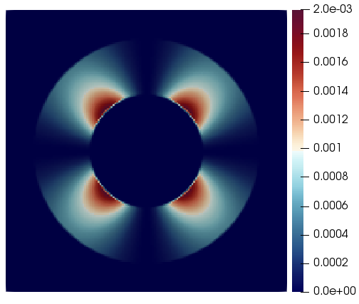
(a) $\hat{\mathcal{E}}^{S}_{u_{n}+a}$

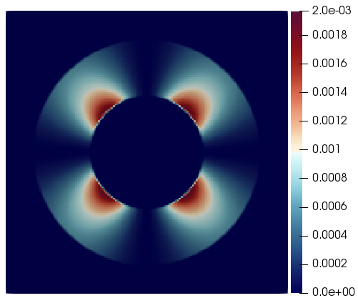
(b) $\hat{\mathcal{E}}^{S}_{u_{n}-a}$

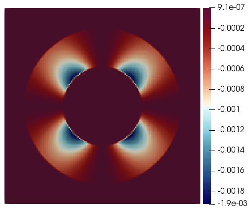
(c) $\hat{\mathcal{E}}_{u_{n}-a,u_{n}+a}$

Figure 28: Gresho Vortex: Entropy production fields along the original acoustic eigenvectors at $t=0$ for the ES Turkel flux. $M_{r}=3\times 10^{-2}$.

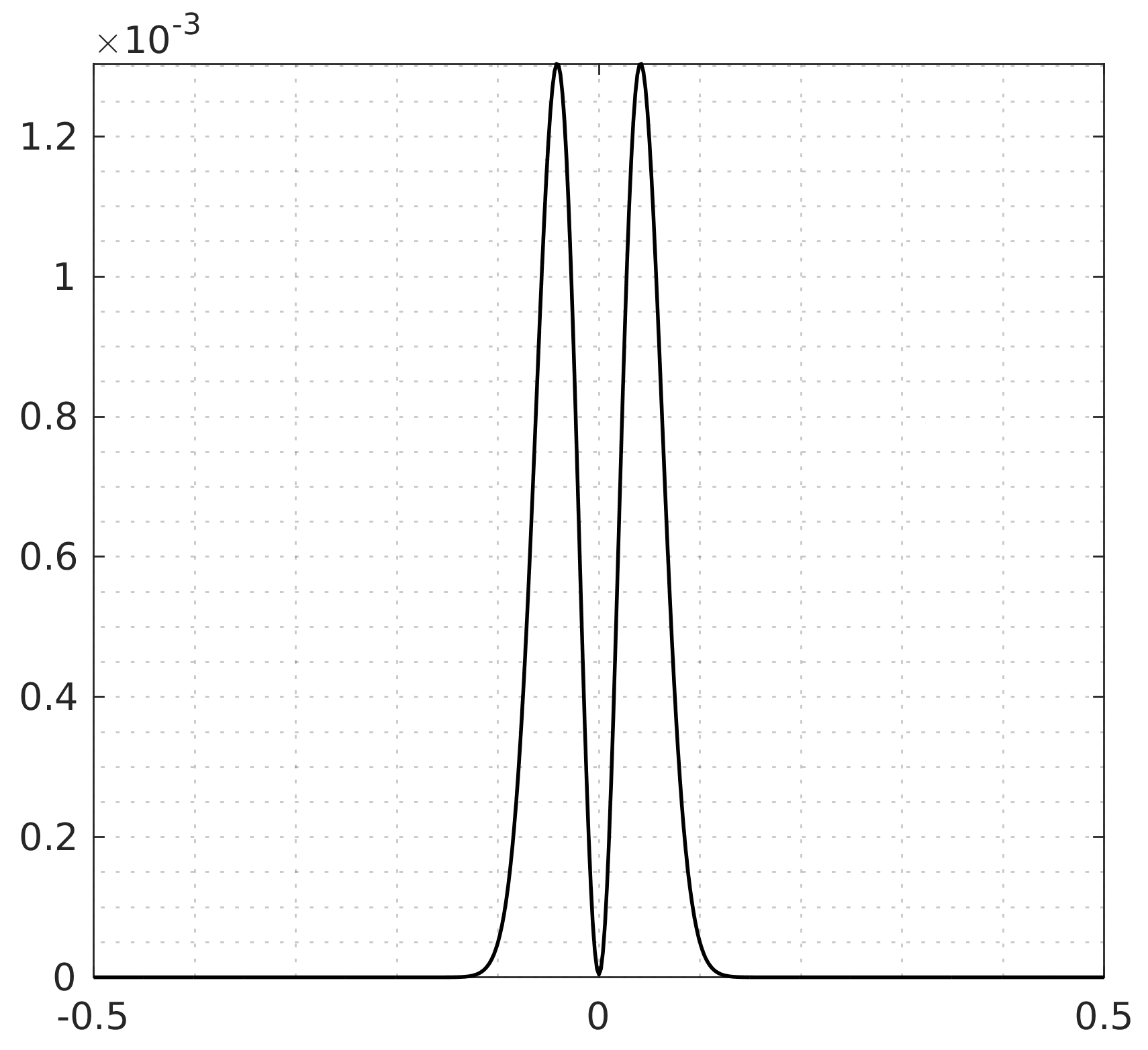
(a) $\hat{\mathcal{E}}^{S}_{u_{n}+a}$

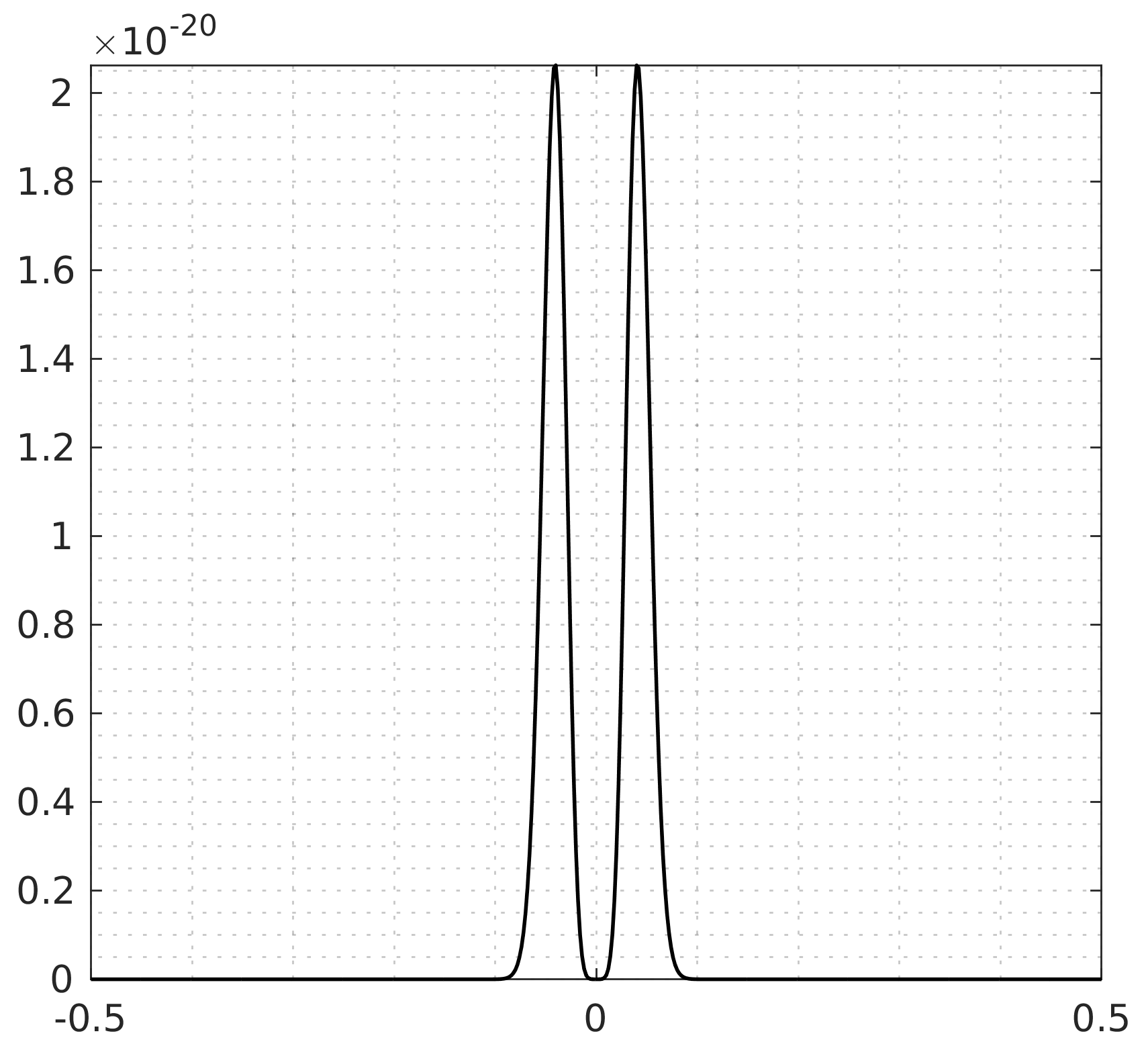
(b) $\hat{\mathcal{E}}^{S}_{u_{n}-a}$

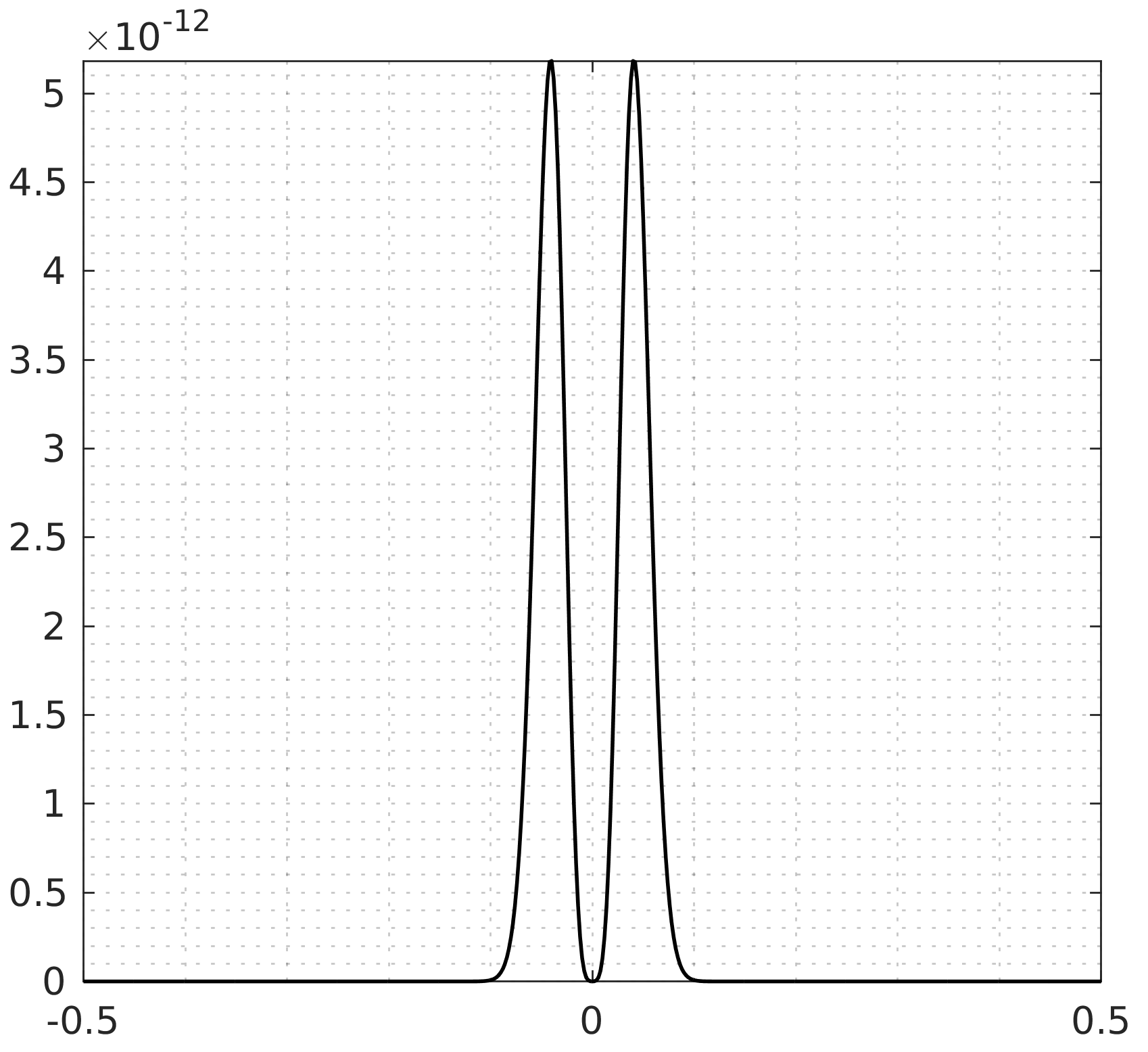
(c) $\hat{\mathcal{E}}_{u_{n}-a,u_{n}+a}$

Figure 30: Sound wave: Entropy production fields along the original acoustic eigenvectors at $t=0$ for the ES Turkel flux $M_{r}=10^{-2}$.

Figures 28 and 30 show the initial entropy production fields for the Gresho vortex and the sound wave using the decomposition (104). These entropy production fields are more similar to those of the classic ES Roe flux (figures 11 and 12) than the ones along the modified acoustic eigenvectors (figures 32 and 33). We also see that the coupling term $\mathcal{E}_{u_{n}+a,u_{n}-a}$ can be negative.
For Miczek’s flux-preconditioner, modified and original acoustic eigenvectors satisfy:

$$\mathbf{r}_{u_{n}+a_{p}}= \ \frac{1}{\sqrt{2}(p^{2}+1)(K_{1}-K_{2})}\bigg{(}\big{(}K_{1}(1+p)+1-p\big{)}\mathbf{r}_{u_{n}+a}+\big{(}K_{1}(1-p)-(1+p)\big{)}\mathbf{r}_{u_{n}-a}\bigg{)},$$

$$\mathbf{r}_{u_{n}-a_{p}}= \ \frac{1}{\sqrt{2}(p^{2}+1)(K_{1}-K_{2})}\bigg{(}\big{(}K_{2}(1+p)+1-p\big{)}\mathbf{r}_{u_{n}+a}+\big{(}K_{2}(1-p)-(1+p)\big{)}\mathbf{r}_{u_{n}-a}\bigg{)}.$$

The new decomposition (102)-(103) writes:

$$\mathcal{E}_{p}\ =\ \big{(}\mathcal{E}^{S}_{u_{n}+a}\ +\ \mathcal{E}_{u_{n}+a,u_{n}-a}\ -\ \Delta\mathcal{E}_{a}\big{)}\ +\ \big{(}\mathcal{E}^{S}_{u_{n}-a}\ +\ \mathcal{E}_{u_{n}-a,u_{n}+a}\ +\ \Delta\mathcal{E}_{a}\big{)}.$$ (105)

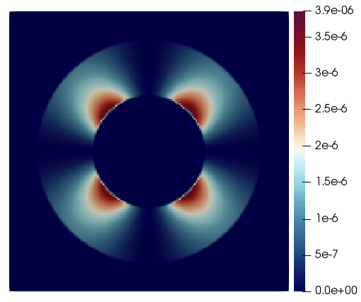
(a) $\hat{\mathcal{E}}^{S}_{u_{n}+a}$

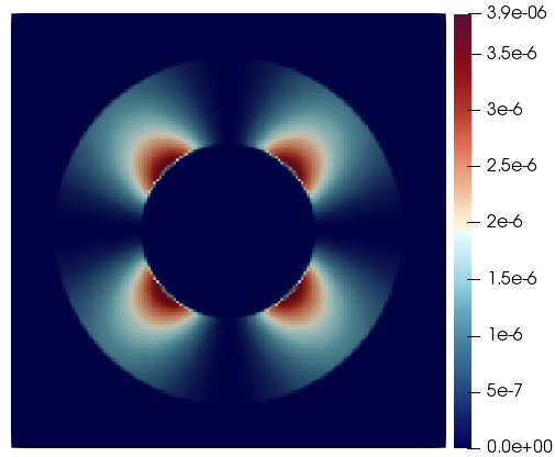
(b) $\hat{\mathcal{E}}^{S}_{u_{n}-a}$

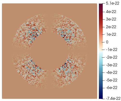
(c) $\hat{\mathcal{E}}_{u_{n}-a,u_{n}+a}$

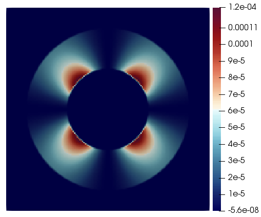
(d) $\Delta\hat{\mathcal{E}}_{a}$

Figure 29: Gresho Vortex: Entropy production fields along the original acoustic eigenvectors at $t=0$ for the ES Miczek flux. $M_{r}=3\times 10^{-2}$.

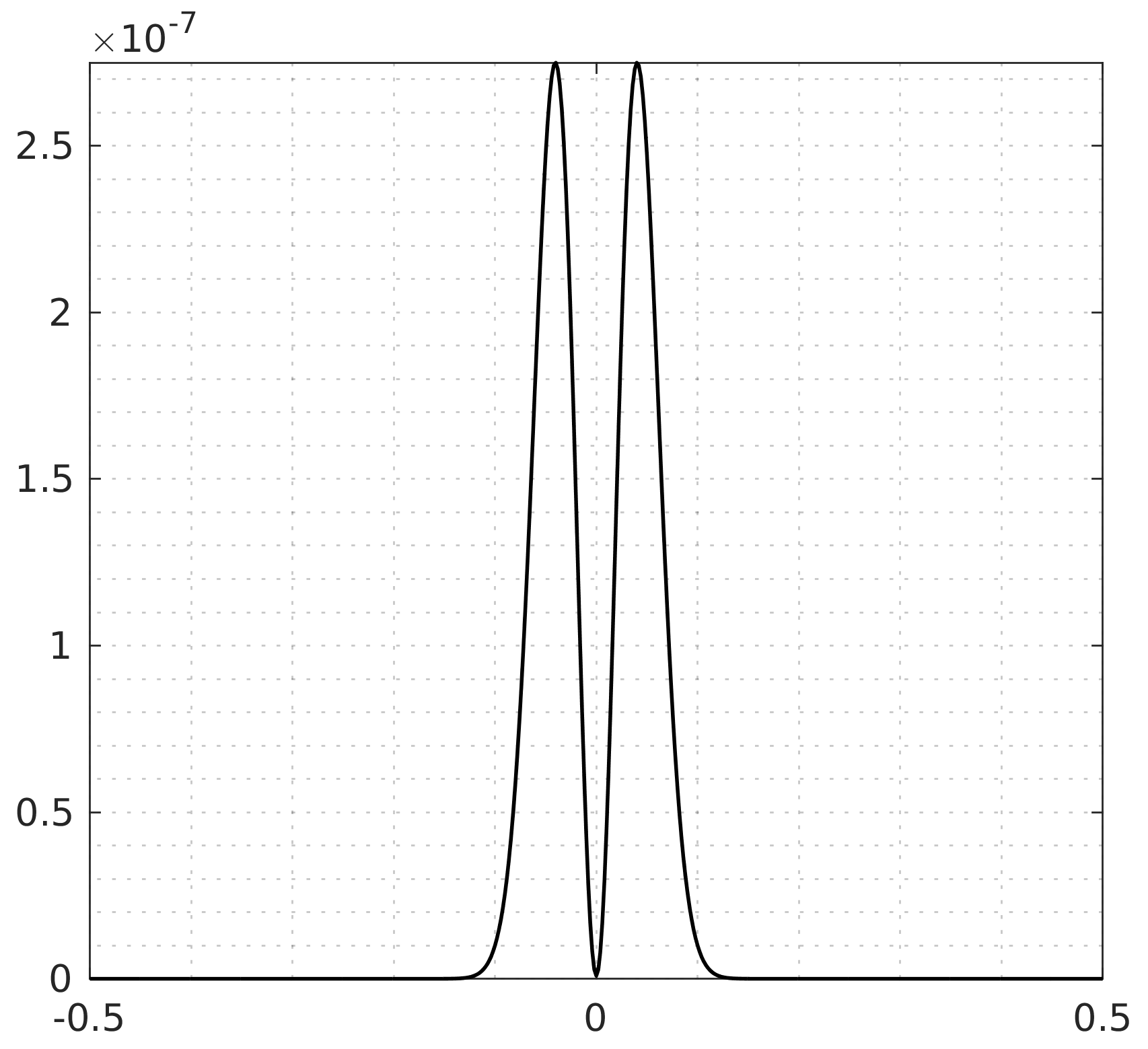
(a) $\hat{\mathcal{E}}^{S}_{u_{n}+a}$

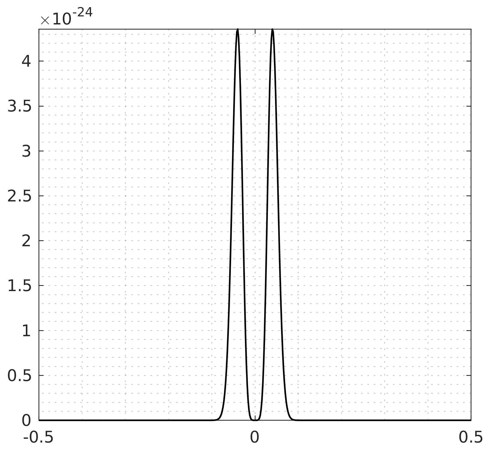
(b) $\hat{\mathcal{E}}^{S}_{u_{n}-a}$

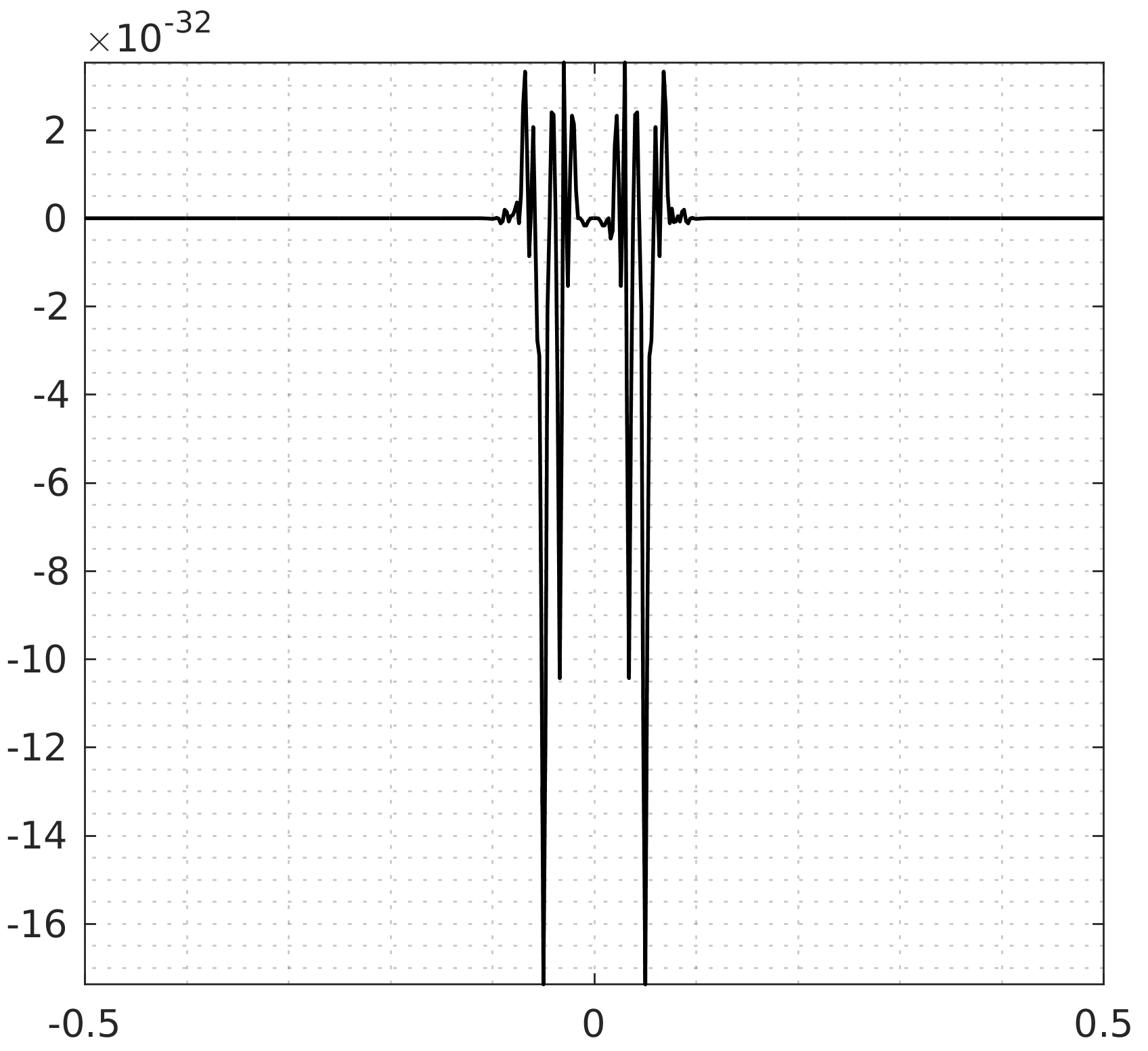
(c) $\hat{\mathcal{E}}_{u_{n}-a,u_{n}+a}$

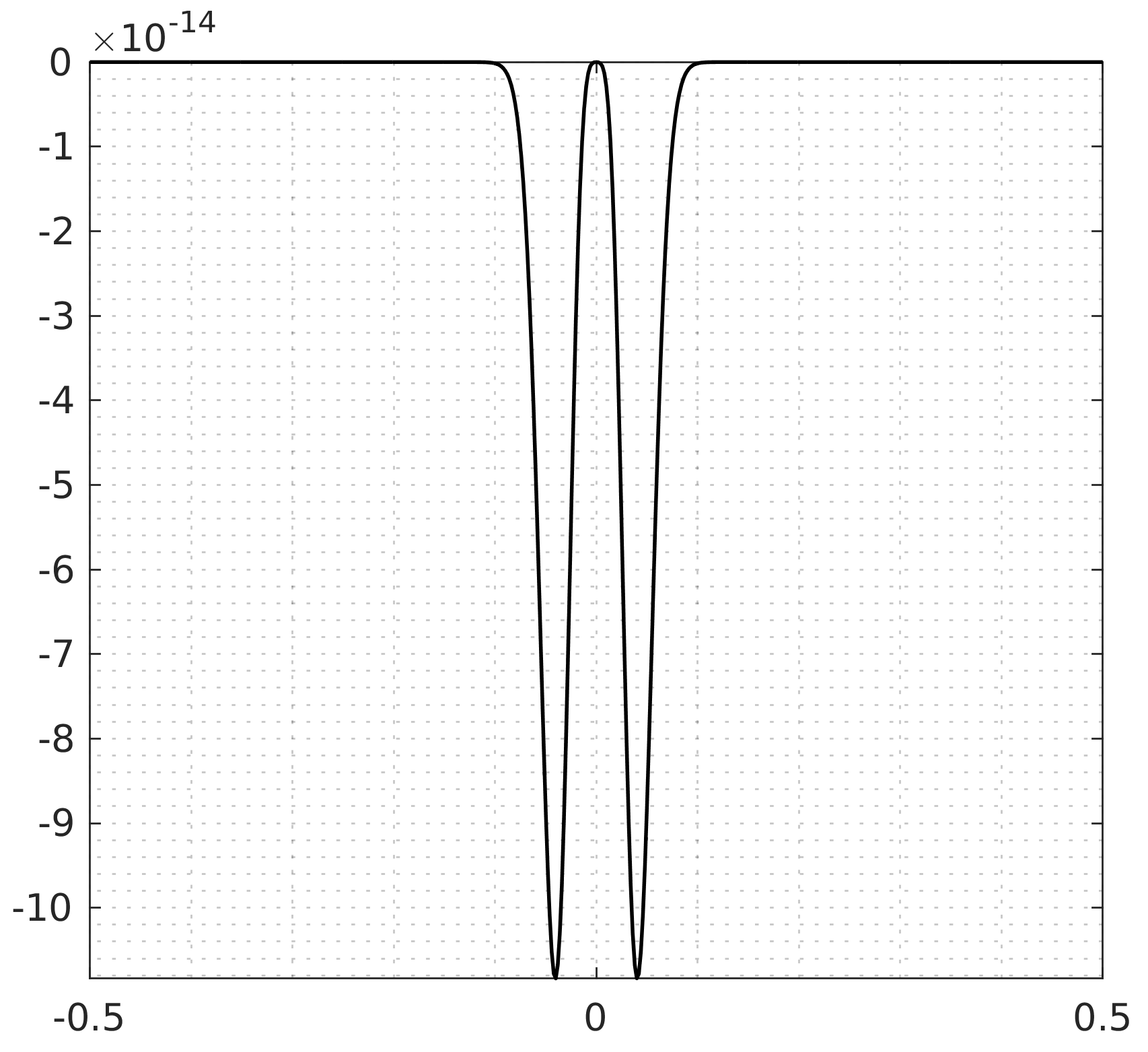
(d) $\Delta\hat{\mathcal{E}}_{a}$

Figure 31: Sound wave: Entropy production fields along the acoustic eigenvectors at $t=0$ for the ES Miczek flux $M_{r}=10^{-2}$.

Figures 29 and 31 show the initial entropy production fields for the Gresho vortex and the sound wave using EPB (105). The coupling term $\mathcal{E}_{u_{n}+a,u_{n}-a}$ is negligible. For the sound wave, figure 25 shows the integrated entropy production fields according to (105). The culpability of the skew-symmetric part of the ES Miczek flux in the spurious transient is striking : the skew-symmetric contribution $\Delta\mathcal{E}_{a}$ kicks in around $t\in\{0,0.5,1\}$. This could not be seen with the previous EPB (figure 18).

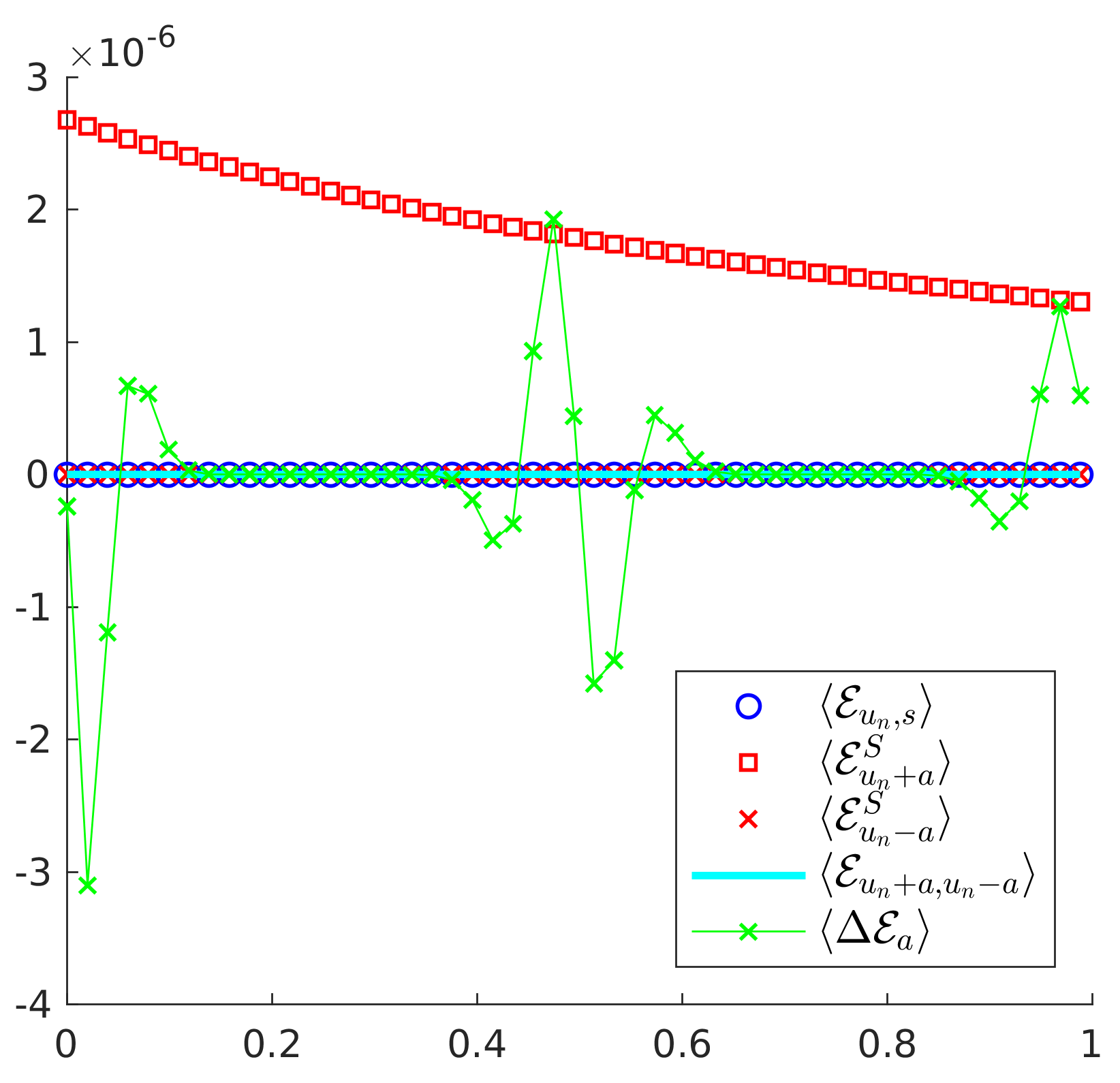
Figure 25: Sound wave: Integral of entropy production fields along the acoustic eigenvectors with time at $M_{r}=10^{-2}$ for the ES Miczek flux.

7.4 An Incomplete Picture

In an unpublished manuscript, Roe ES_Roe2 made the following observation regarding EC fluxes:

Corollary 7.0.1 (Roe ES_Roe2 ).

Let $\mathbf{f}_{EC}^{*}$ an EC flux following theorem (4.1). Then for any skew-symmetric matrix $\Delta$, we have that the numerical flux $\mathbf{f^{*}}$ defined by:

$$\mathbf{f^{*}}\ =\ \mathbf{f}_{EC}^{*}\ -\ \Delta[\mathbf{v}],$$ (106)

is EC as well.

This result is a simple consequence of $[\mathbf{v}]^{T}\Delta[\mathbf{v}]=0$. While $\Delta$ does not contribute to the total discrete entropy production, it still has an impact on the discrete entropy equation (47) through the entropy flux $F^{*}$. It is easy to show that the discrete entropy flux writes:

$$F^{*}=\overline{\mathbf{v}}\cdot\big{(}\mathbf{f^{*}}-\Delta[\mathbf{v}]\big{)}-\overline{\mathcal{F}}.$$

The contribution from $\Delta$ is non-zero. We ran the skewed ES flux of section 7.2 without $R|\Lambda_{p}|R^{T}[\mathbf{v}]$ (this leaves a skewed EC flux (106)) and observed the same anomalies (figures 26 and 27). This shows that the picture drawn by EPBs is not complete, and that perhaps we should take a few steps back and try to better understand discrete entropy conservation first.
In section 4.2 we got a glimpse of how diverse EC fluxes can be. EC fluxes such as Roe’s (4.2) or Chandrasekhar’s (4.2) are popular because of their algebraic simplicity but their local behavior is not easy to analyze, at least analytically. Given a dissipation operator $R|\Lambda|R^{T}[\mathbf{v}]=\sum_{k=1}^{N}\mathbf{r}_{k}|\Lambda_{k}|\mu_{k}$, one could look for an EC flux $\mathbf{f^{*}}$ of the form:

$$\mathbf{f^{*}}=\sum_{k=1}^{N}f_{k}\mathbf{r}_{k}\ \implies\ [\mathbf{v}]\cdot\mathbf{f^{*}}=\sum_{k=1}^{N}f_{k}\mu_{k}$$

Following theorem 4.1, the implied sum above has to be equal to the jump $[\mathcal{F}]$. If $[\mathcal{F}]$ can be broken down as the sum of $N$ independent intermediate jumps $[\mathcal{F}]^{k}$, then one can solve for the $f_{k}^{*}$ and obtain the candidate EC flux:

$$f_{k}\ =\ \frac{[\mathcal{F}]^{k}}{\mu_{k}}\ \implies\ \mathbf{f^{*}}\ =\ \sum_{k=1}^{N}\bigg{(}\frac{[\mathcal{F}]^{k}}{\mu_{k}}\bigg{)}\ \mathbf{r}_{k}.$$ (107)

This candidate flux qualifies if it is consistent. This kind of modal EC flux was already introduced by Tadmor ES_Tadmor_2003 about two decades ago. He set $[\mathcal{F}]^{k}=\mathcal{F}(\mathbf{v}^{*,k+1})-\mathcal{F}(\mathbf{v}^{*,k})$ with an appropriately designed sequence $\big{(}\mathbf{v}^{*,k}\big{)}_{1\leq k\leq N+1}$ satisfying $\mathbf{v}^{*,1}=\mathbf{v}_{L}$, $\mathbf{v}^{*,N+1}=\mathbf{v}_{R}$. This modal representation might lead to useful insights into the local behavior of EC fluxes. One could for instance compare the magnitudes of the $f_{k}$ coefficients and use skew-symmetric interface operators $R\Delta R^{T}[\mathbf{v}]$ to alter the balance $\ \sum_{k=1}^{N}\mu_{k}f_{k}=[\mathcal{F}]\$ and see how it effects the discrete solution.
When considering the anomalies associated with the ES Miczek flux in the second test problem, we talked about entropy transfer between (acoustic) waves. It is important to recognize that for nonlinear flow configurations involving significant discontinuities and/or multi-dimensional physics, the notion of a wave become ambiguous. One can argue that the EPBs we introduced and worked with are inherently one-dimensional.
Regarding the effect of the temporal discretization on discrete entropy dynamics, we could introduce a temporal EPB starting from $\mathcal{E}^{BE}$ (eq. (61) - theorem 4.3) and using $H=RR^{T}$ (corollary 4.4.1) but computing the fields accurately requires quadrature. In addition, they cannot be computed a priori. Elements of discussion regarding the effect of temporal discretization can be found in Gouasmi_0 ; Gouasmi_1 .

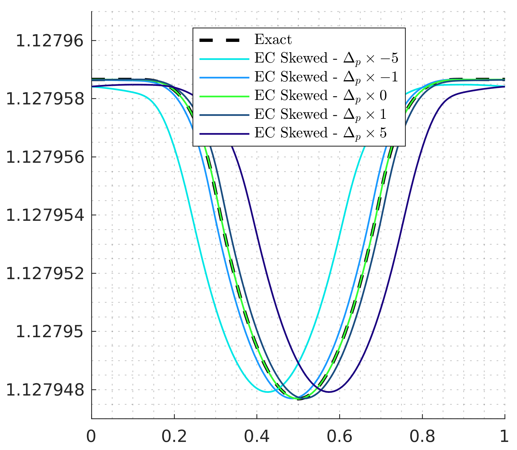
(a) $t=1$

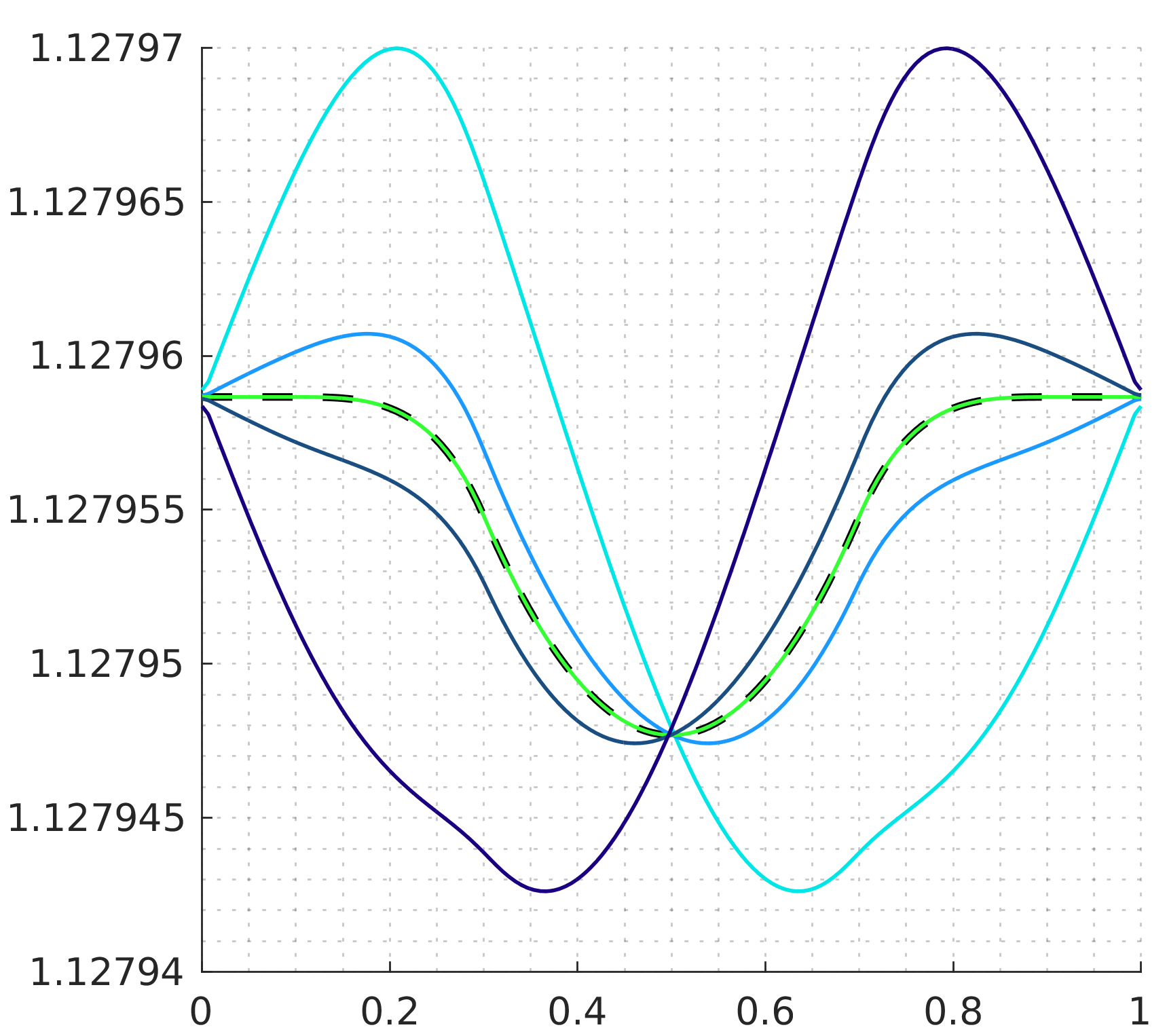
(b) $t=0.04$

Figure 26: Gresho Vortex: Centerline pressure profile with the skewed EC flux. $M_{r}=3\times 10^{-3}$.

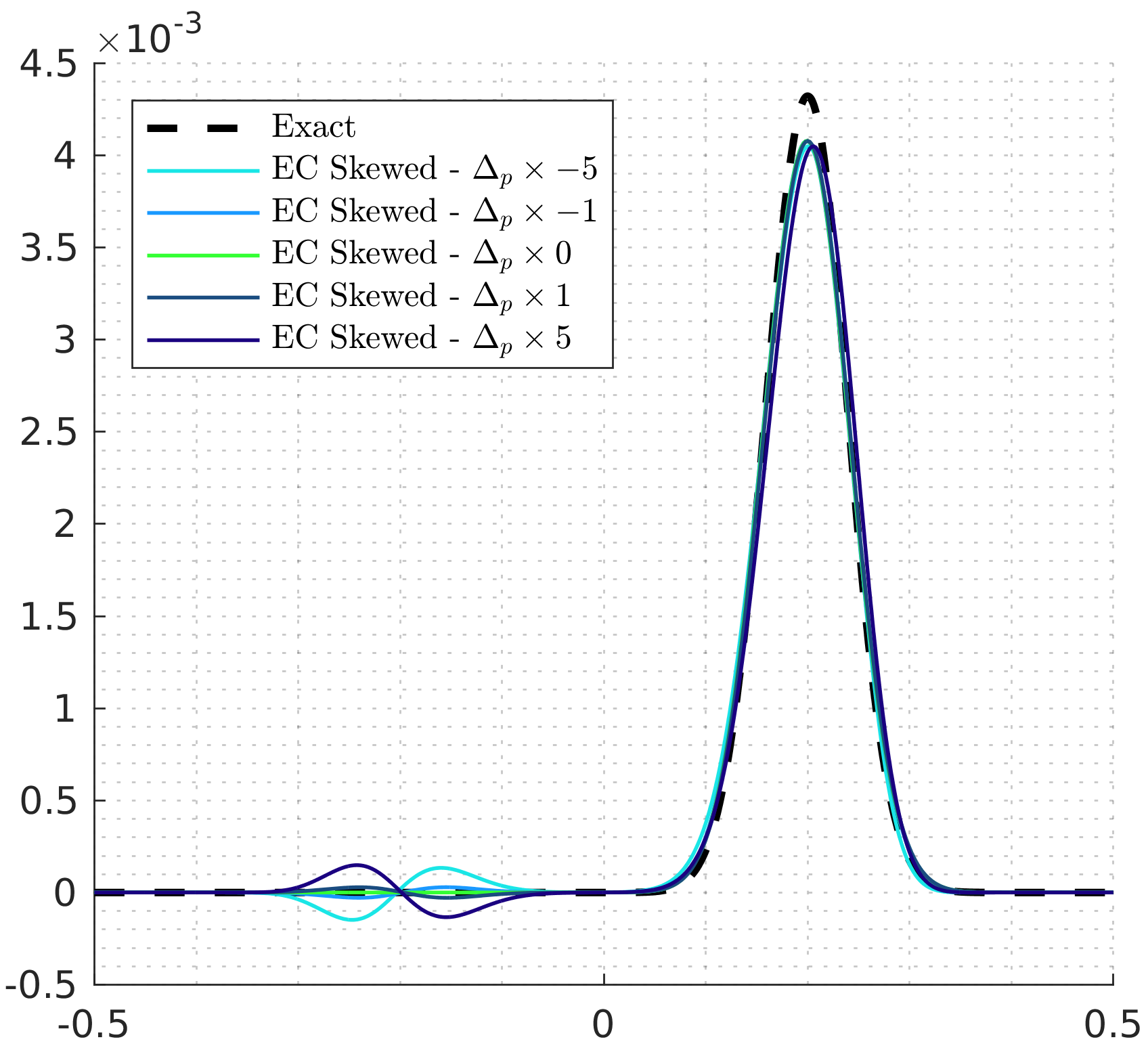
(a) $t=0.03$

(b) $t=0.03$, zoomed

Figure 27: Sound wave: Same pressure profiles as in figure 19 with the skewed EC flux instead. $M_{r}=10^{-2}$.

8 Conclusions

In this work, the behavior of ES schemes in the low-Mach regime was investigated. We showed that standard ES schemes suffer from the same accuracy degradation issues as standard upwind schemes (and for the same reasons). Using appropriate similarity and congruence transforms, we were able to define the extent to which the flux-preconditioning technique is compatible with entropy-stability. We introduced ES versions of the preconditioned upwind fluxes of Turkel and Miczek. Numerical results confirmed the analysis but also highlighted spurious transients with the flux-preconditioner of Miczek which were not reported until now.
These unexpected anomalies, together with the recent work of Bruel et al. Bruel on the acoustic limit and the failure of the Turkel flux-preconditioner, led us to further investigate the matter. Leveraging Tadmor’s framework, we introduced discrete Entropy Production Breakdowns (EPBs) that allowed us to revisit the accuracy degradation issue in terms of entropy. In the same spirit as Guillard & Viozat Guillard1 (incompressible limit) and Bruel et al. Bruel (acoustic limit), we showed that the accuracy degradation problems at the discrete level are caused by discrete entropy fluctuations that are inconsistent with those of the continuous system.
An important outgrowth of the overall effort is the discovery that the spurious transients observed with the ES Miczek flux are caused by a skew-symmetric dissipation term which appeared when a scaled form $R|\Lambda|R^{T}[\mathbf{v}]$ of the preconditioned dissipation operator was sought. Analytical and numerical arguments suggest that this term induces entropy transfers between acoustic waves. While the role played by skew-symmetric terms and the scope of EPBs remain to be fully understood, we believe these findings shed new lights on the local behavior of EC/ES schemes and how to further improve them. These findings should also, hopefully, convince the reader that there is more to draw from EC/ES schemes than a global stability statement such as inequality (3).
Future work will continue the analysis in a more complex setting, including unstructured grids Bader , high-order discretizations and mixed flow configurations Thornber2 of practical interest. The challenges associated with efficient time-integration and preconditioning (stiffness and steady-state convergence Turkel2005 ) will bring yet another layer of difficulty to that effort.

A Entropy Production Field Snapshots

(a) $\hat{\mathcal{E}}_{u_{np}+a_{p}}$

(a) $\hat{\mathcal{E}}_{u_{np}+a_{p}}=\hat{\mathcal{E}}^{S}_{u_{np}+a_{p}}-\Delta\hat{\mathcal{E}}_{p}$

(b) $\hat{\mathcal{E}}_{u_{np}-a_{p}}=\hat{\mathcal{E}}^{S}_{u_{np}-a_{p}}+\Delta\hat{\mathcal{E}}_{p}$

(c) $\hat{\mathcal{E}}^{S}_{u_{np}+a_{p}}$

(a) $\hat{\mathcal{E}}_{u_{np}+a_{p}}=\hat{\mathcal{E}}^{S}_{u_{np}+a_{p}}-\Delta\hat{\mathcal{E}}_{p}$

(b) $\hat{\mathcal{E}}_{u_{np}-a_{p}}=\hat{\mathcal{E}}^{S}_{u_{np}+a_{p}}+\Delta\hat{\mathcal{E}}_{p}$

(c) $\hat{\mathcal{E}}^{S}_{u_{np}+a_{p}}$

(d) $\hat{\mathcal{E}}^{S}_{u_{np}-a_{p}}$

(e) $\Delta\hat{\mathcal{E}}_{p}$

Figure 35: Sound wave: Entropy production fields at $t=0$ for the ES Miczek flux. $M_{r}=10^{-2}$.

References

- (1) Klainerman, S., and Majda, A. : Compressible and Incompressible Fluids, Commun. Pure Appl. Math, 35, pp. 629-651, 1982.
- (2) Schochet, S. : The mathematical theory of low Mach number flows, ESAIM-Math. Model. Num., 39 (3), pp. 441-458, 2005.
- (3) Turkel, E. : Preconditioning Techniques in Computational Fluid Dynamics, Annu. Rev. Fluid Mech., 31, pp.385-416, 1999.
- (4) Turkel, Preconditioned Methods for Solving the Incompressible and Low Speed Compressible Equations, J. Comput. Phys., 72(2), pp. 277-298, 1987.
- (5) Turkel, E., Fiterman, A., and van Leer B. : Pre-conditioning and the limit to the incompress-ible flow equations, In: Computing the Future: Frontiers of Computational Fluid Dynamics, ed. DA Caughey, MM Hafez, pp. 215–34. New York: Wiley, 1994.
- (6) Turkel, E., and Vatsa, V.N. : Local Preconditioners for Steady State and Dual Time-Stepping, ESAIM-Math. Model. Num. 39 (3), pp. 515-536, 2005.
- (7) G. Volpe, Performance of compressible flow codes at low Mach numbers, AIAA Journal, 31(1), 1993.
- (8) Rieper, F., and Bader, G. : The influence of cell geometry on the accuracy of upwind schemes in the low mach number regime, J. Comput. Phys. 228 (8), pp. 2918-2933, 2009.
- (9) Gresho, P.M., and Chan, S.T. : On the theory of semi‐implicit projection methods for viscous incompressible flow and its implementation via a finite element method that also introduces a nearly consistent mass matrix. Part 2: Implementation, Int. J. Numer. Fl., 11 (5), pp. 1990.
- (10) Liska, R., and Wendroff, B. : Comparison of several difference schemes on 1D and 2D test problems for the Euler equations, SIAM J. Sci. Comput. 25 (3), pp. 995–1017, 2003.
- (11) Miczek, F. : Simulation of low Mach number astrophysical flows, PhD Thesis, Technical University of Munich, 2013.
- (12) Miczek, F., Ropke, F.K., and Edelmann, P.V.F. : New numerical solver for flows at various Mach numbers, A&A, 576, A50 (2015).
- (13) Barsukow, W., Edelmann, P.V.F., Klingenberg, C., Miczek, F., and Röpke, F.K. : A numerical scheme for the compressible low-Mach number regime of ideal fluid dynamics, J. Sci. Comput., 72(2), pp 623–646, 2017.
- (14) Guillard, H. and Viozat, C.: On the Behavior of Upwind Schemes in the Low Mach Number Limit, Comput. Fluids 28, pp. 63-86, 1999.
- (15) Guillard, H., and Nkonga, B. : On the Behavior of Upwind Schemes in the Low Mach Number limit: A Review, chapter 8 in Handbook of Numerical Analysis 18, 2017.
- (16) Guillard, H., and Murrone, A. : On the behavior of upwind schemes in the low Mach number limit: II. Godunov type schemes, Comput. Fluids 33(4), pp. 655-675, 2004.
- (17) Chorin, A.J. : A Numerical Method for Solving Incompressible Viscous Flow Problems, J. Comput. Phys. 135(2), pp. 118-125, 1967.
- (18) Weiss, J.M., and Smith, W.A. : Preconditioning applied to variable and constant density flows, AIAA Journal, 33(11), pp. 2050-2057, 1995.
- (19) Klein, R. : Semi-implicit extension of a godunov-type scheme based on low mach number asymptotics I: One-dimensional flow, J. Comput. Phys. 121 (2), pp. 213-237, 1995.
- (20) Van Leer, B., Lee, W-T., and Roe, P. L. : Characteristic time-stepping or local preconditioning of the Euler equations, AIAA-1991-1552, AIAA Computational Fluid Dynamics Conference, 1991.
- (21) Merkle, C. and Choi, Y. : Computation of Low Speed Compressible Flows with Time-Marching Methods, Int. J. Numer. Meth. Eng., 25, pp. 293–311, 1985.
- (22) Li, X.S., and Gu, C.W. : An all-speed Roe-type scheme and its asymptotic analysis of low Mach number behavior, J. Comput. Phys. 227 (10), pp. 5144-5159, 2008.
- (23) Li, X.S., and Gu, C.W. : Mechanism of Roe-type schemes for all-speed flows and its application, Comput. Fluids 38 (4), pp. 810-817, 2009.
- (24) Birken, B., and Meister, A. : Stability of Preconditioned Finite Volume schemes at low Mach numbers, BIT Numer. Math., 45(3), pp. 463-480, 2005.00
- (25) Thornber, B., Drirakis, D., Williams, R.J.R, and Youngs, D. : On entropy generation and dissipation of kinetic energy in high-resolution shock-capturing schemes, J. Comput. Phys., 227 (10) pp. 4853-4872, 2008.
- (26) Thornber, B., Mosedale, A., Drirakis, D., Williams, R.J.R, and Youngs, D. : An improved reconstruction method for compressible flows with low Mach number features, J. Comput. Phys., 227 (10) pp. 4873-4894, 2008.
- (27) Dellacherie, S. : Analysis of Godunov type schemes applied to compressible Euler system at low Mach numbers, J. Comput. Phys., 229 (4), pp. 978-1016, 2010.
- (28) Rieper, F. : A low-Mach number fix for Roe’s approximate Riemann solver, J. Comput. Phys., 230 (13), pp. 5263-5287, 2011.
- (29) Oßwald, K., Siegmund, A., Birken, P., Hannemann, V., and Meister, A. : L2Roe: a low dissipation version of Roe’s approximate Riemann solver for low Mach numbers, Int. J. Numer. Meth. Fl., 81, pp. 71–86, 2016.
- (30) Bruel, P., Delmas, S., Jung, J., and Perrier, V. : A low Mach correction able to deal with low Mach acoustics, J. Comput. Phys., 378 pp. 723-759, 2019.
- (31) Friedrichs, K. O., and Lax, P. D. : Systems of Conservation Equations with a Convex Extension, P. Natl. Acad. Sci. U.S.A, 68 (8) pp. 1686-1688, 1971.
- (32) Lax, P.D. : Shock Waves and Entropy, In: E. Zarantonello, Ed., Contributions to Nonlinear Functional Analysis, Academia Press, New York, 1971, pp. 603-634.
- (33) Harten, A. : On the symmetric form of systems of conservation laws with entropy, J. Comput. Phys. 49 (1), pp. 151-164, 1983.
- (34) Harten, A., Lax, P. D., Levermore C. D., and Morokoff, W. J. : Convex entropies and hyperbolicity for general Euler equations, SIAM J. Numer. Anal., 33 (6) pp. 2117-2127, 1998.
- (35) Hughes, T.J.R, Franca, L.P., and Mallet, M. : A new finite element formulation for computational fluid dynamics: I. Symmetric forms of the compressible Euler and Navier-Stokes equations and the second law of thermodynamics, Comput. Method. Appl. M. 54(2), pp. 223-234, 1986.
- (36) Mock, M. S. : Systems of conservation laws of mixed type, J. Differ. Equations 70 (1), pp. 70-88, 1980.
- (37) Tadmor, E. : The numerical viscosity of entropy stable schemes for systems of conservation laws, I, Math. Comput. 49, pp. 91-103, 1987.
- (38) Tadmor, E. : Entropy stability theory for difference approximations of nonlinear conservation laws and related time-dependent problems, Acta Numer., 12, pp. 451-512, 2003.
- (39) Barth, T.J. : Numerical Methods for Gasdynamic Systems on Unstructured Meshes. In: Kröner D., Ohlberger M., Rohde C. (eds) An Introduction to Recent Developments in Theory and Numerics for Conservation Laws. Lecture Notes in Computational Science and Engineering, vol 5. Springer, Berlin, Heidelberg, 1999.
- (40) Merriam, M. : An Entropy-Based Approach to Nonlinear Stability, NASA Technical Memorandum, 1989.
- (41) Roe, P. L., and Pike, J. : Efficient Construction and Utilisation of Approximate Riemann Solutions, Computing Methods in Applied Science and Engineering, INRIA North-Holland, pp. 499-518, 1984.
- (42) Roe, P.L. : Approximate Riemann solvers, parameter vectors, and difference schemes, J. Comput. Phys. 72 pp. 357–372, 1987.
- (43) Roe, P.L.: Affordable, entropy consistent flux functions. In: Eleventh International Conference on Hyperbolic Problems: Theory, Numerics and Applications, 2006.
- (44) Roe, P.L. : Affordable, Entropy-consistent, Euler Flux Functions: I. Analytical Results, University of Michigan, Unpublished, 2007.
- (45) Ismail, F., and Roe, P.L. : Affordable, entropy-consistent Euler flux functions II: Entropy production at shocks, J. Comput. Phys., 228 (15) pp. 5410-5436, 2009.
- (46) Chandrasekhar, P. : Kinetic energy preserving and entropy stable finite volume schemes for compressible Euler and Navier–Stokes equations, Commun. Comput. Phys. 14, pp. 1252–1286, 2013.
- (47) Fjordholm, U.S., Mishra, S., and Tadmor, E. : Arbitrarily High-order Accurate Entropy Stable Essentially Nonoscillatory Schemes for Systems of Conservation Laws, SIAM J. Numer. Anal., 50 (2) pp. 544-573, 2012.
- (48) Diosady, L. T., and Murman, S. M. : Higher-Order Methods for Compressible Turbulent Flows Using Entropy Variables, 53rd AIAA Aerospace Sciences Meeting, 2015.
- (49) Murman, S.M., Diosady, L.T., Garai, A., and Ceze, M. : A Space-Time Discontinuous-Galerkin Approach for Separated Flows, 54th AIAA Aerospace Sciences Meeting, 2016.
- (50) Carton de Wiart, C., Diosady, L.T., Garai, A., Burgess, N., Blonigan, P., and Murman, S.M. : Design of a modular monolithic implicit solver for multi-physics applications, AIAA SciTech Forum, 2018.
- (51) Fisher, T.C. and Carpenter, M.H. : High-order entropy stable finite difference schemes for nonlinear conservation laws: Finite domains, J. Comput. Phys., 252(1) pp 518-557, 2013.
- (52) Friedrich, L., Schnücke, G., Winters, A.R., Del Rey Fernández, D.C., Gassner, G. J., and Carpenter, M.H. : Entropy Stable Space–Time Discontinuous Galerkin Schemes with Summation-by-Parts Property for Hyperbolic Conservation Laws, J. Sci. Comput., 2019.
- (53) Pazner, W., and Persson, P-O : Analysis and Entropy Stability of the Line Based Discontinuous Galerkin Method, J. Sci. Comput., 80 (1) pp. 376-402, 2019.
- (54) Fernandez, P., Nguyen, N-C, and Peraire, J. : Entropy-stable hybridized discontinuous Galerkin methods for the compressible Euler and Navier-Stokes equations, arXiv:1808.05066, 2018.
- (55) Slotnick J, Khodadoust A, Alonso J, Darmofal D, Gropp W, et al. : CFD Vision 2030 study: a path to revolutionary computational aerosciences. NASA Tech. Rep. CR-2014-218178, Langley Res. Cent., Hampton, VA.
- (56) Gottlieb, S., Shu, C.W., and Tadmor E. : Strong stability-preserving high-order time discretization methods, SIAM Rev., 43 (1), 2001, pp. 89-112
- (57) Guermond, J.L., Nazarov, M., Popov, B., Tomas, I. : Second-order invariant domain preserving approximation of the Euler equations using convex limiting, SIAM J. Sci. Comput. 40 (5), pp. 3211–3239, 2018.
- (58) Guermond, J.-L., Popov, B., and Tomas, I. : Invariant domain preserving discretization-independent schemes and convex limiting for hyperbolic systems, Comput. Method. Appl. M. 347, pp. 143-175, 2019.
- (59) Knoll, A., and Keyes, D.E. : Jacobian-free Newton–Krylov methods: a survey of approaches and applications, J. Comp. Phys. 193(2), pp. 357-397, 2004.
- (60) Gouasmi, A. : Contributions to the Development of Entropy-Stable Schemes for Compressible Flows, PhD Thesis, University of Michigan, 2020.
- (61) Gouasmi, A., Murman, S.M. & Duraisamy, K. : Entropy Conservative Schemes and the Receding Flow Problem, J. Sci. Comput. 78, pp. 971–994, 2019.
- (62) Gouasmi, A., Duraisamy, K. & Murman, S.M. : On entropy-stable temporal fluxes, arXiv:1807.03483, 2018.
- (63) Gouasmi, A., Duraisamy, K. & Murman, S.M. : Formulation of Entropy-Stable Schemes for Compressible Multi-Component Euler equations, Comput. Method. Appl. M., 363, 112912, 2020.
- (64) Gouasmi, A., Duraisamy, K., Murman, S.M. & Tadmor. E. : A minimum entropy principle in the compressible multicomponent Euler equations, ESAIM-Math. Model. Num. 54, pp. 373–389, 2020.
- (65) Gouasmi, A., Duraisamy, K., Murman, S.M. : On the Behavior of Entropy Stable Schemes in the Low Mach Regime, in 16th U.S. National Congress on Computational Mathematics, NASA Technical Report Server 20210018590, 2021.