Double Trouble: How to not Explain a Text Classifier’s Decisions Using Counterfactuals Synthesized by Masked Language Models?

Double Trouble: How to not Explain a Text Classifier’s Decisions Using Counterfactuals Synthesized by Masked Language Models?

Abstract

A principle behind dozens of attribution methods is to take the prediction difference between before-and-after an input feature (here, a token) is removed as its attribution. A popular Input Marginalization (IM) method Kim et al. (2020) uses BERT${}_{\text{$\mathsf{}$}}$ to replace a token, yielding more plausible counterfactuals. While Kim et al. (2020) reported that IM is effective, we find this conclusion not convincing as the Deletion${}_{\text{$\mathsf{BERT}$}}$ metric used in their paper is biased towards IM. Importantly, this bias exists in Deletion-based metrics, including Insertion, Sufficiency, and Comprehensiveness. Furthermore, our rigorous evaluation using 6 metrics and 3 datasets finds no evidence that IM is better than a Leave-One-Out (LOO) baseline. We find two reasons why IM is not better than LOO: (1) deleting a single word from the input only marginally reduces a classifier’s accuracy; and (2) a highly predictable word is always given near-zero attribution, regardless of its true importance to the classifier. In contrast, making Local Interpretable Model-Agnostic Explanations (LIME) counterfactuals more natural via BERT consistently improves LIME accuracy under several RemOve-And-Retrain (ROAR) metrics.

1 Introduction

(a) SST – Groundtruth & target class: “positive”
S	The very definition of the ‘ small ’ movie , but it is a good stepping stone for director Sprecher .
	0.9793 stepping      0.9760 stone         0.8712 for
	0.0050 rolling           0.0048 stones         0.0860 to
	0.0021 casting          0.0043 point           0.0059 ,
IM0	The very definition of the ‘ small ’ movie , but it is a good stepping stone for director Sprecher .
IM1	The very definition of the ‘ small ’ movie , but it is a good stepping stone for director Sprecher .
IM2	The very definition of the ‘ small ’ movie , but it is a good stepping stone for director Sprecher .
IM3	The very definition of the ‘ small ’ movie , but it is a good stepping stone for director Sprecher .
(b) e-SNLI – Groundtruth & target class: “contradiction”
P	A group of people prepare hot air balloons for takeoff .
	0.9997 hot               0.9877 air            0.9628 balloons
	0.0001 compressed   0.0102 water         0.0282 balloon
	0.0000 open              0.0008 helium       0.0019 engines
H	A group of people prepare cars for racing .
IM0	A group of people prepare hot air balloons for takeoff .
	A group of people prepare cars for racing .
IM1	A group of people prepare hot air balloons for takeoff .
	A group of people prepare cars for racing .
IM2	A group of people prepare hot air balloons for takeoff .
	A group of people prepare cars for racing .
IM3	A group of people prepare hot air balloons for takeoff .
	A group of people prepare cars for racing .

Figure 1: By design, IM erroneously assigns near-zero attribution to highly-predictable words. Color map: negative -1, neutral 0, positive +1. Many words labeled important by humans such as “stepping”, “stone” (a) or “hot”, “air” (b) are always given near-zero attribution by IM (because they are highly predictable by BERT, e.g. 0.9793 for stepping) regardless of the classifier. Even when randomizing the classifier’s weights three times, the IM attribution of these words remains unchanged at near zero (IM₁ to IM₃). Therefore, when marginalizing over the top-$k$ BERT candidates (e.g., “stepping”, “rolling”, “casting”), the IM attribution for low-entropy words tends to zero, leading to heatmaps that are biased, less accurate, and less plausible than LOO${}_{\text{$\mathsf{empty}$}}$.

Feature attribution maps (AMs), i.e. highlights indicating the importance of each input token w.r.t. a classifier’s decision, can help improve human accuracy on downstream tasks including detecting fake movie reviews Lai and Tan (2019) or identifying biases in text classifiers Liu and Avci (2019).

Many Leave-One-Out (LOO) methods compute the attribution of an input token by measuring the prediction changes after substituting that token’s embedding with zeros Li et al. (2016); Jin et al. (2020) or [UNK] Kim et al. (2020). That is, deleting or replacing features is the underlying principle of at least 25 attribution methods Covert et al. (2020).

Based on the evidence in computer vision Bansal et al. (2020); Zhang et al. (2019), prior works in NLP hypothesized that removing a word from an input text forms out-of-distribution (OOD) inputs that yield erroneous AMs Kim et al. (2020); Harbecke and Alt (2020) or AMs inconsistent with human’s perception of causality Hase et al. (2021). To generate plausible counterfactuals, two teams of researchers Kim et al. (2020); Harbecke and Alt (2020) proposed Input Marginalization (IM), i.e. replace a word using BERT${}_{\text{$\mathsf{}$}}$ Devlin et al. (2019) and compute an average prediction difference by marginalizing over all predicted words. Kim et al. (2020) claimed that IM yields more accurate AMs than the baselines that replace words by [UNK] or zeros but their quantitative results were reported for only one dataset and one evaluation metric.

In this paper, we re-assess their claim by, first, reproducing their IM results, and then rigorously evaluate whether improving the realism of counterfactuals improves two attribution methods (LOO and LIME). On a diverse set of three datasets and six metrics, we find that:

1. The Deletion${}_{\text{$\mathsf{BERT}$}}$ metric in Kim et al. (2020) is biased towards IM as both use BERT to replace words (Sec. 4). In contrast, the vanilla Deletion metric Arras et al. (2017) favors the LOO${}_{\text{$\mathsf{empty}$}}$ baseline as both delete words. This bias causes a false conclusion that IM is better than LOO baselines in Kim et al. (2020) and also exists in other Deletion variants, e.g., Insertion Arras et al. (2017), Sufficiency, and Comprehensiveness DeYoung et al. (2020).

2. We find no evidence that IM is better than a simple LOO${}_{\text{$\mathsf{empty}$}}$ on any of the following four state-of-the-art AM evaluation metrics (which exclude the biased Deletion & Deletion${}_{\text{$\mathsf{BERT}$}}$): ROAR, ROAR${}_{\text{$\mathsf{BERT}$}}$ Hooker et al. (2019) (Sec. 5.1), comparison against human annotations (Sec. 5.2), and sanity check Adebayo et al. (2018) (Sec. 5.3).

3. We argue that IM is not effective in practice because: (1) deleting a single word from an input has only a marginal effect on classification accuracy (Sec. 5.4); and (2) given a perfect, masked language model $G$, IM would still be unfaithful because highly predictable words according to $G$, e.g. “hot”, “air” in Fig.1, are always assigned near-zero attribution in IM regardless of how important they are to the classifier (Sec. B).

4. To further test the main idea of IM, we integrate BERT into LIME Ribeiro et al. (2016) to replace multiple words (instead of deleting) in an input sequence, making LIME counterfactuals more realistic. We find this technique to improve LIME consistently under multiple ROAR-based metrics, but not under comparison against human annotations (Sec. 6).

To our knowledge, our work is the first to thoroughly study the effectiveness of IM in NLP in both settings of replacing a single word (LOO) and multiple words (LIME). Importantly, we find improvement in the latter but not the former setting.

2 Methods and Related Work

Let $f\mathrel{\mathop{\mathchar 58\relax}}{\mathbb{R}}^{n\times d}\to[0,1]$ be a text classifier that maps a sequence ${\bm{x}}$ of $n$ token embeddings, each of size $d$, onto a confidence score of an output label. An attribution function $A$ takes three inputs—a sequence ${\bm{x}}$, the model $f$, and a set of hyperparameters ${\mathcal{H}}$—and outputs a vector ${\bm{a}}=A(f,{\bm{x}},{\mathcal{H}})\in[-1,1]^{n}$. Here, the explanation ${\bm{a}}$ associates each input token $x_{i}$ to a scalar $a_{i}\in[-1,1]$, indicating how much $x_{i}$ contributes for or against the target label.

Leave-One-Out

(LOO) is a well-known method Li et al. (2016); Robnik-Šikonja and Kononenko (2008); Jin et al. (2020) for estimating the attribution $a_{i}$ by computing the prediction-difference after a token $x_{i}$ is left out of the input ${\bm{x}}$, creating a shorter sequence ${\bm{x}}_{-i}$:

$$a_{i}=f({\bm{x}})-f({\bm{x}}_{-i})$$ (1)

Under Pearl (2009) causal framework, the attribution $a_{i}$ in Eq. 1 relies on a single, unrealistic counterfactual ${\bm{x}}_{-i}$ and thus is a biased estimate of the individual treatment effect (ITE):

ITE $$=f({\bm{x}})-\mathbb{E}[f({\bm{x}})\mid do(T=0)]$$ (2)

where the binary treatment $T$, here, is to keep or “realistically remove” the token $x_{i}$ (i.e. $T=1$ or $0$) in the input ${\bm{x}}$, prior to the computation of $f({\bm{x}})$.

Perturbation techniques

In computer vision (CV), earlier attribution methods erase a feature by replacing it with (a) zeros Zeiler and Fergus (2014); Ribeiro et al. (2016); (b) random noise Dabkowski and Gal (2017); Lundberg and Lee (2017); or (c) blurred versions of the original content Fong et al. (2019). Yet, these perturbation methods produce unrealistic counterfactuals that make AMs more unstable and less accurate Bansal et al. (2020).

Recent works proposed to simulate the $do(T=0)$ operator using an image inpainter. However, they either generated unnatural counterfactuals Chang et al. (2019); Goyal et al. (2019) or only a single, plausible counterfactual per example Agarwal and Nguyen (2020).

Input marginalization (IM)

In NLP, IM${}_{\text{$\mathsf{}$}}$ offers the closest estimate of the ITE. IM computes the $\mathbb{E}[.]$ term in Eq. 2 by marginalizing over many plausible counterfactuals generated by BERT${}_{\text{$\mathsf{}$}}$:

$$\mathbb{E}[f({\bm{x}})\mid ~{}do(T=0)]$$

$$=\sum_{\tilde{x}_{i}\in{{\mathcal{V}}}}p(\tilde{x}_{i}|{\bm{x}}_{-i})\cdot f({\bm{x}}_{-i},\tilde{x}_{i})$$ (3)

where $\tilde{x}_{i}$ is a token suggested by BERT${}_{\text{$\mathsf{}$}}$ (e.g., “hot”, “compressed”, or “open” in Fig. 1) with a likelihood of $p(\tilde{x}_{i}|{\bm{x}}_{-i})$ to replace the masked token $x_{i}$. ${\mathcal{V}}$ is the BERT${}_{\text{$\mathsf{}$}}$ vocabulary of 30,522 tokens. $f({\bm{x}}_{-i},\tilde{x}_{i})$ is the classification probability when token $x_{i}$ in the original input is replaced with $\tilde{x}_{i}$.

IM attribution is in the $\log$ space:

$$a_{\text{IM}} =\text{log-odds}(f({\bm{x}}))$$

$$~{}~{}~{}~{}~{}-\text{log-odds}(\mathbb{E}[f({\bm{x}})\mid do(T=0)])$$ (4)

where $\text{log-odds}(p)=\log_{2}(p/(1-p))$.

As computing the expectation in Eq. 3 over BERT’s $\sim$30K-word vocabulary is prohibitively slow, IM authors only marginalized over the words that have a likelihood $\geq 10^{-5}$. We are able to reproduce the IM${}_{\text{$\mathsf{}$}}$ results of Kim et al. (2020) by taking only the top-10 words. That is, using the top-10 words or all words of likelihood $\geq 10{-5}$ yields slightly different numbers but the same conclusions (Sec. D). Thus, we marginalize over the top-10 for all experiments. Note that under BERT, the top-10 tokens, on average, already account for $81\%$, $90\%$, and $92\%$ of the probability mass for SST-2, e-SNLI, & MultiRC, respectively.

BERT

Like Kim et al. (2020), we use a pre-trained BERT${}_{\text{$\mathsf{}$}}$ “base”, uncased model (Devlin et al., 2019), from Huggingface (2020), to fill in a [MASK] token to generate counterfactuals in IM.

LIME

Based on the idea of IM, we also integrate BERT${}_{\text{$\mathsf{}$}}$ into LIME${}_{\text{$\mathsf{}$}}$, which originally masks out multiple tokens at once to compute attribution. LIME${}_{\text{$\mathsf{}$}}$ generates a set of randomly masked versions of the input, and the attribution of a token $x_{i}$, is effectively the mean classification probability over all the masked inputs when $x_{i}$ is not masked out. On average, each vanilla LIME${}_{\text{$\mathsf{}$}}$ counterfactual has 50% of tokens taken out, yielding text often with large syntactic and grammatical errors.

LIME${}_{\text{$\mathsf{BERT}$}}$

We use BERT to replace multiple masked tokens in each masked sentence generated by LIME to construct more plausible counterfactuals. However, for each word, we only use the top-1 highest-likelihood token given by BERT instead of marginalizing over multiple tokens because (1) the full marginalization is prohibitively slow; and (2) the top-1 token already carries most of the weight ($p\geq 0.81$; see Table A3).

3 Experiment framework

3.1 Three datasets

We select a diverse set of three classification datasets that enable us to (1) compare with the results reported by Kim et al. (2020); and (2) assess AMs on six evaluation metrics (described in Sec. 3.3). These three tasks span from sentiment analysis (SST-2), natural language inference (e-SNLI) to question answering (MultiRC), covering a wide range of sequence length ($\sim$20, 24, and 299 tokens per example, respectively). SST-2 and e-SNLI were the two datasets where Kim et al. (2020) found IM${}_{\text{$\mathsf{}$}}$ to be superior to LOO baselines.

SST

Stanford Sentiment Treebank (Socher et al., 2013b) is a dataset of $\sim$12K RottenTomato movie-review sentences, which contain human-annotated sentiment annotations for phrases. Each phrase and sentence in SST is assigned a sentiment score $\in[0,1]$ (0 = negative, 0.5 = neutral, 1 = positive).

SST-2

has $\sim$70K SST examples (including both phrases and sentences) where the regression scores per example were binarized to form a binary classification task Socher et al. (2013b).

e-SNLI

A 3-way classification task of detecting whether the relation between a premise and a hypothesis is entailment, neutral or contradiction Bowman et al. (2015). e-SNLI has 569K instances of (input, label, explanation) where the explanations are crowd-sourced Camburu et al. (2018).

MultiRC

Multi-sentence Reading Comprehension (Khashabi et al., 2018) is a multiple-choice question-answering task that provides multiple input sentences as well as a question and asks the model to select one or multiple correct answer sentences. MultiRC has $\sim$6K examples with human-annotated highlights at the sentence level.

3.2 Classifiers

Following Kim et al. (2020); Harbecke and Alt (2020); Hase et al. (2021), we test IM${}_{\text{$\mathsf{}$}}$ and LOO baselines in explaining BERT-based classifiers.

For each task, we train a classifier by fine-tuning the entire model, which consists of a classification layer on top of the pre-trained BERT (described in Sec. 2). The dev-set top-1 accuracy scores of our SST-2, e-SNLI, & MultiRC classifiers are 92.66%, 90.92%, and 69.10%, respectively. On the SST binarized dev-set, which contains only sentences, the SST-2-trained classifier’s accuracy is 87.83%.

Hyperparameters

Following the training scheme of HuggingFace, we fine-tune all classifiers for 3 epochs using Adam optimizer (Kingma and Ba, 2015) with a learning rate of 0.00002, $\beta_{1}$ = 0.9, $\beta_{2}$ = 0.999, $\epsilon=10^{-8}$. A batch size of 32 and a max sequence length of 128 are used for SST-2 and e-SNLI while these hyperparameters for MultiRC are 8 and 512, respectively. Dropout with a probability of 0.1 is applied to all layers. Each model was trained on an NVIDIA 1080Ti GPU.

3.3 Six evaluation metrics

As there are no groundtruth explanations in XAI, we use six common metrics to rigorously assess IM’s effectiveness. For each classifier, we evaluate the AMs generated for all dev-set examples.

Deletion   is similar to “Comprehensiveness” DeYoung et al. (2020) and is based on the idea that deleting a token of higher importance from the input should cause a larger drop in the output confidence score. We take the original input and delete one token at a time until 20% of the tokens in the input is deleted. A more accurate explanation is expected to have a lower Area Under the output-probability Curve (AUC) Arras et al. (2017).

Deletion${}_{\text{$\mathsf{BERT}$}}$   a.k.a. AUC${}_{\text{$\mathsf{rep}$}}$ in Kim et al. (2020), is a Deletion variant where a given token is replaced by a BERT top-1 suggestion instead of an empty string. Deletion${}_{\text{$\mathsf{BERT}$}}$ was proposed to minimize the OOD-ness of samples (introduced by deleting words in the vanilla Deletion metric), i.e. akin to integrating BERT into LOO to create IM.

RemOve And Retrain (ROAR)   To avoid a potential OOD${}_{\text{$\mathsf{}$}}$ generalization issue caused by the Deletion metric, a common alternative is to retrain the classifier on these modified inputs (where $N$% of the highest-attribution words are deleted) and measure its accuracy drop Hooker et al. (2019). A more faithful attribution method is supposed to lead to a re-trained classifier of lower accuracy as the more important words have been deleted from training examples. For completeness, we also implement ROAR${}_{\text{$\mathsf{BERT}$}}$, which uses BERT to replace the highest-attribution tokens instead of deleting them without replacement in ROAR.

Agreement with human-annotated highlights   In both CV and NLP, a common AM evaluation metric is to assess the agreement between AMs and human annotations Wiegreffe and Marasović (2021). The idea is that as text classifiers well predict the human labels of an input text, their explanations, i.e. AMs, should also highlight the tokens that humans deem indicative of the groundtruth label.

Because human annotators only label the tokens supportive of a label (e.g. Fig. 2), when comparing AMs with human annotations, we zero out the negative values in AMs. Following Zhou et al. (2016), we binarize a resulting AM at an optimal threshold $\tau$ in order to compare it with human-annotated highlights under Precision@1.

Sanity check   Adebayo et al. (2018) is a well-known metric for testing insensitivity (i.e. bias) of attribution methods w.r.t. model parameters. For ease of interpretation, we compute the % change of per-word attribution values in sign and magnitude as we randomize the classification layer’s weights. A better attribution method is expected to be more sensitive to the classifier’s weight randomization.

4 Bias of Deletion metric and its variants

In explaining SST-2 classifiers, we successfully reproduce the AUC${}_{\text{$\mathsf{rep}$}}$ results reported in Kim et al. (2020), i.e. IM${}_{\text{$\mathsf{}$}}$ outperformed LOO${}_{\text{$\mathsf{zero}$}}$ and LOO${}_{\text{$\mathsf{unk}$}}$, which were implemented by replacing a word with the [PAD] and [UNK] token of BERT, respectively (Table 1). However, we hypothesize that Deletion${}_{\text{$\mathsf{BERT}$}}$ is biased towards IM as both use BERT to replace words, yielding a false sense of IM effectiveness reported in Kim et al. (2020).

To test this hypothesis, we add another baseline of LOO${}_{\text{$\mathsf{empty}$}}$, which was not included in Kim et al. (2020), i.e. erasing a token from the input without replacement (Eq. 1), mirroring the original Deletion metric. To compare with IM${}_{\text{$\mathsf{}$}}$, all LOO methods in this paper are also in the log-odds space.

Results   Interestingly, we find that, under Deletion, on both SST-2 and e-SNLI, IM${}_{\text{$\mathsf{}$}}$ underperformed all three LOO baselines and that LOO${}_{\text{$\mathsf{empty}$}}$ is the highest-performing method (Table 1a). In contrast, IM${}_{\text{$\mathsf{}$}}$ is the best method under Deletion${}_{\text{$\mathsf{BERT}$}}$.

Re-running the same experiment but sampling replacement words from RoBERTa (instead of BERT), we find the same finding that LOO${}_{\text{$\mathsf{empty}$}}$ is the best under Deletion while IM is the best under Deletion${}_{\text{$\mathsf{BERT}$}}$ (Table 1b).

Task	Metrics $\downarrow$	IM${}_{\text{$\mathsf{}$}}$	LOO${}_{\text{$\mathsf{zero}$}}$	LOO${}_{\text{$\mathsf{unk}$}}$	LOO${}_{\text{$\mathsf{empty}$}}$
(a) BERT${}_{\text{$\mathsf{}$}}$
SST-2	Deletion	0.4732	0.4374	0.4464	0.4241
	Deletion${}_{\text{$\mathsf{BERT}$}}$	0.4922	0.4970	0.5047	0.5065
e-SNLI	Deletion	0.3912	0.2798	0.3742	0.2506
	Deletion${}_{\text{$\mathsf{BERT}$}}$	0.2816	0.3240	0.3636	0.3328
(b) RoBERTa${}_{\text{$\mathsf{}$}}$
SST-2	Deletion	0.4981	0.4524	0.4595	0.4416
	Deletion${}_{\text{$\mathsf{BERT}$}}$	0.4798	0.5037	0.5087	0.4998

Table 1: IM is the best method under Deletion${}_{\text{$\mathsf{BERT}$}}$, as reported in Kim et al. (2020), but the worst under Deletion. Both metrics measure AUC (lower is better).

To our knowledge, our work is the first to document this bias of the Deletion metric widely used in the literature Hase et al. (2021); Wiegreffe and Marasović (2021); Arras et al. (2017). This bias, in principle, also exists in other Deletion variants including Insertion Arras et al. (2017), Sufficiency, and Comprehensiveness DeYoung et al. (2020).

5 No evidence that IM is better than LOO

To avoid the critical bias of Deletion and Deletion${}_{\text{$\mathsf{BERT}$}}$, we further compare IM and LOO on four common metrics that are not Deletion-based.

5.1 Under ROAR and ROAR${}_{\text{$\mathsf{BERT}$}}$, IM is on-par with or worse than LOO${}_{\text{$\mathsf{empty}$}}$

A lower AUC under Deletion may be the artifact of the classifier misbehaving under the distribution shift when one or multiple input words are deleted. ROAR Hooker et al. (2019) was designed to ameliorate this issue by re-training the classifier on a modified training-set (where the top $N\%$ highest-attribution tokens in each example are deleted) before evaluating their accuracy.

To more objectively assess IM${}_{\text{$\mathsf{}$}}$, we use ROAR and ROAR${}_{\text{$\mathsf{BERT}$}}$ metrics to compare IM${}_{\text{$\mathsf{}$}}$ vs. LOO${}_{\text{$\mathsf{empty}$}}$ (i.e. the best LOO variant in Table 1).

Experiment   For both IM${}_{\text{$\mathsf{}$}}$ and LOO${}_{\text{$\mathsf{empty}$}}$, we generate AMs for every example in the SST-2 train and dev sets, and remove $N\%$ highest-attribution tokens per example to create new train and dev sets. We train 5 models on the new training set and evaluate them on the new dev set. We repeat ROAR and ROAR${}_{\text{$\mathsf{BERT}$}}$ with $N\in\{10,20,30\}$.

Results   As more tokens are removed (i.e. $N$ increases), the mean accuracy of 5 models gradually decreases (Table 5.1; from 92.66% to $\sim$67%). Under both ROAR and ROAR${}_{\text{$\mathsf{BERT}$}}$, the models trained on the new training set derived from LOO${}_{\text{$\mathsf{empty}$}}$ AMs often obtain lower (i.e. better) mean accuracy than those of IM${}_{\text{$\mathsf{}$}}$ (Table 5.1a vs. b). At $N=10\%$ under ROAR, LOO${}_{\text{$\mathsf{empty}$}}$ outperforms IM (Table 5.1; 74.59 vs. 76.22), which is statistically significant (2-sample $t$-test, $p=0.037$). In all other cases, the difference between IM vs. LOO${}_{\text{$\mathsf{empty}$}}$ is not statistically significant.

In sum, under both ROAR and ROAR${}_{\text{$\mathsf{BERT}$}}$, IM is not more faithful than LOO${}_{\text{$\mathsf{empty}$}}$.

lcccc|ccc Accuracy in % (lower is better) ROAR ROAR${}_{\text{$\mathsf{BERT}$}}$
Method $N=0$% 10% 20% 30% 10% 20% 30%
(a) LOO${}_{\text{$\mathsf{empty}$}}$ 92.62 $\pm$ 0.30 74.59 $\pm$ 0.78 68.94 $\pm$ 1.46 67.89 $\pm$ 0.79 76.79 $\pm$ 0.56 71.95 $\pm$ 0.75 67.62 $\pm$ 1.16
(b) IM${}_{\text{$\mathsf{}$}}$ 92.62 $\pm$ 0.30 76.22 $\pm$ 1.18 70.07 $\pm$ 0.69 66.54 $\pm$ 1.89 77.36 $\pm$ 0.90 71.56 $\pm$ 1.55 67.68 $\pm$ 0.96
(c) Random 92.62 $\pm$ 0.30 89.22 $\pm$ 0.53 87.75 $\pm$ 0.19 85.62 $\pm$ 0.53 89.38 $\pm$ 0.47 88.23 $\pm$ 0.31 85.21 $\pm$ 0.47
(d) $t$-test p-value N/A 0.0370 0.1740 0.1974 0.2672 0.6312 0.9245

Table 2: Dev-set mean accuracy (%) of 5 models trained on the new SST-2 examples where $N$% of highest-attribution words per example are removed (i.e. ROAR) or replaced via BERT (i.e. ROAR${}_{\text{$\mathsf{BERT}$}}$). On average, under both metrics, LOO${}_{\text{$\mathsf{empty}$}}$ (a) is slightly better, i.e. lower mean accuracy, than IM${}_{\text{$\mathsf{}$}}$ (b). Notably, LOO${}_{\text{$\mathsf{empty}$}}$ statistically significantly outperforms IM${}_{\text{$\mathsf{}$}}$ under ROAR at $N=10$% (2-sample $t$-test; $p=0.037$) (d). Both LOO${}_{\text{$\mathsf{empty}$}}$ and IM${}_{\text{$\mathsf{}$}}$ substantially outperform a random baseline (c) that considers $N\%$ random tokens important.

ccc|ccc|cc|cc|cc Metric $\uparrow$ (a) SST (b) e-SNLI   L2 (c) e-SNLI   L3 (d) MultiRC
Higher is better IM${}_{\text{$\mathsf{}$}}$ LOO${}_{\text{$\mathsf{empty}$}}$ LIME${}_{\text{$\mathsf{}$}}$ LIME${}_{\text{$\mathsf{BERT}$}}$ LIME${}_{\text{$\mathsf{BERT\_SST2}$}}$ IM${}_{\text{$\mathsf{}$}}$ LOO${}_{\text{$\mathsf{empty}$}}$ IM${}_{\text{$\mathsf{}$}}$ LOO${}_{\text{$\mathsf{empty}$}}$ IM${}_{\text{$\mathsf{}$}}$ LOO${}_{\text{$\mathsf{empty}$}}$

IoU 0.2377 0.2756 0.3193 0.3170 0.3127 0.3316 0.3415 0.2811 0.3411 0.0437 0.0887
precision 0.5129 0.4760 0.4831 0.4629 0.4671 0.4599 0.4867 0.3814 0.4687 0.1784 0.1940
recall 0.5245 0.6077 0.6882 0.7000 0.6886 0.6085 0.6158 0.5699 0.5875 0.0630 0.2876
F1 0.5186 0.5338 0.5677 0.5573 0.5566 0.5239 0.5437 0.4570 0.5214 0.0931 0.2317

Table 3: Compared to IM${}_{\text{$\mathsf{}$}}$, LOO${}_{\text{$\mathsf{empty}$}}$ is substantially more consistent with human annotations over all three datasets. Note that the gap between LOO${}_{\text{$\mathsf{empty}$}}$ and IM${}_{\text{$\mathsf{}$}}$ is $\sim$$3\times$ wider when comparing AMs with the e-SNLI tokens that at least three annotators label “important” (i.e. L3), compared to L2 (higher is better). LIME${}_{\text{$\mathsf{BERT}$}}$ explanations are slightly less consistent with human highlights than those of LIME (a) despite their counterfactuals are more realistic.

5.2 LOO${}_{\text{$\mathsf{empty}$}}$ aligns significantly better with human annotations than IM

Following Wiegreffe and Marasović (2021), to increase our understanding of the differences between LOO${}_{\text{$\mathsf{empty}$}}$ and IM, we compare the two methods against the human-annotated highlights for SST, e-SNLI, and MultiRC.

Annotation preprocessing   To control for quality, we preprocess the human annotations in each dataset as the following. In SST, where each sentence has multiple phrases labeled with a sentiment score $\in[0,1]$ (0.5 being the “neutral” midpoint), we only use the phrases that have high-confidence sentiment scores, i.e. $\leq 0.3$ (for “negative”) or $\geq 0.7$ (for “positive”). Also, we do not use the annotated phrases that are too long, i.e., longer than 50% of the sentence length.

Each token in an e-SNLI example are labeled “important” by between 0–3 annotators. To filter out noise, we only use the tokens that are highlighted by at least two or three annotators (hereafter “L2” and “L3” subsets, respectively).

A MultiRC example contains a question and a paragraph where each sentence is labeled “important” or “unimportant” to the groundtruth answer (Fig. A10). We convert these sentence-level highlights into token-level highlights to compare them with the binarized AMs of IM and LOO${}_{\text{$\mathsf{empty}$}}$.

Experiment   We run IM${}_{\text{$\mathsf{}$}}$ and LOO${}_{\text{$\mathsf{empty}$}}$ on the BERT-based classifiers on the dev set of SST, e-SNLI, and MultiRC. All AMs generated are binarized using a threshold $\tau\in\{0.05x\mid 0<x<20\text{ and }x\in\mathbb{N}\}$. We compute the average IoU, precision, recall, and F1 over pairs of (human binary map, binarized AM) and report the results at the optimal $\tau$ of each explanation method. For both LOO${}_{\text{$\mathsf{empty}$}}$ and IM${}_{\text{$\mathsf{}$}}$, $\tau=0.1$ on SNLI-L2 and 0.05 on both SST-2 and MultiRC. On SNLI-L3, $\tau$ is 0.40 and 0.45 for LOO${}_{\text{$\mathsf{empty}$}}$ and IM${}_{\text{$\mathsf{}$}}$, respectively.

SST results   We found that LOO${}_{\text{$\mathsf{empty}$}}$ aligns better with human highlights than IM${}_{\text{$\mathsf{}$}}$ (Figs. 2 & A12). LOO${}_{\text{$\mathsf{empty}$}}$ outperforms IM${}_{\text{$\mathsf{}$}}$ in both F1 and IoU scores (Table 5.1a; 0.2756 vs 0.2377) with a notably large recall gap (0.6077 vs. 0.5245).

SST  Groundtruth & Prediction: “positive” movie review
Input	Mr. Tsai is a very original artist in his medium , and What Time Is It There ?
IM	Mr. Tsai is a very original artist in his medium , and What Time Is It There ?
	IoU: 0.17, precision: 0.33, recall: 0.25
LOO	Mr. Tsai is a very original artist in his medium , and What Time Is It There ?
	IoU: 0.80, precision: 0.80, recall: 1.00

Figure 2: LOO${}_{\text{$\mathsf{empty}$}}$ binarized attribution maps align better with human highlights than IM maps.

e-SNLI and MultiRC results   Similarly, in both tasks, LOO${}_{\text{$\mathsf{empty}$}}$ explanations are more consistent with human highlights than IM${}_{\text{$\mathsf{}$}}$ explanations under all four metrics (see Table 5.1b–d and qualitative examples in Figs. 3 & A13–A16).

Remarkably, in MultiRC where each example is substantially longer ($\sim$299 tokens per example) than those in the other tasks, the recall and F1 scores of LOO${}_{\text{$\mathsf{empty}$}}$ is, respectively, 2$\times$ and 4$\times$ higher than those of IM${}_{\text{$\mathsf{}$}}$ (see Table 5.1).

e-SNLI example.  Groundtruth & Prediction: “entailment”
P	Two men dressed in black practicing martial arts on a gym floor .
H	Two men are doing martial arts .
IM	Two men dressed in black practicing martial arts on a gym floor .
	Two men are doing martial arts .
	IoU: 0.09, precision: 0.17, recall: 0.16
LOO	Two men dressed in black practicing martial arts on a gym floor .
	Two men are doing martial arts .
	IoU: 0.50, precision: 0.56, recall: 0.83

Figure 3: LOO${}_{\text{$\mathsf{empty}$}}$ important words are in a stronger agreement with human highlights than IM important words. Each e-SNLI example contains a pair of premise (P) and hypothesis (H).

5.3 IM is insensitive to model randomization

Adebayo et al. (2018) found that many attribution methods can be surprisingly biased, i.e. insensitive to even randomization of the classifier’s parameters. Here, we test the degree of insensitivity of IM when the last classification layer of BERT-based classifiers is randomly re-initialized. We use three SST-2 classifiers and three e-SNLI classifiers.

Surprisingly, IM is consistently worse than LOO${}_{\text{$\mathsf{empty}$}}$, i.e. more insensitive to classifier randomization. That is, on average, the IM attribution of a word changes signs (from positive to negative or vice versa) less frequently, e.g. 62.27% of the time, compared to 71.41% for LOO${}_{\text{$\mathsf{empty}$}}$ on SST-2 (Table A5a). The average change in attribution magnitude of IM is also $\sim$1.5$\times$ smaller than that of LOO${}_{\text{$\mathsf{empty}$}}$ (Table A5b).

For example, the IM attribution scores of hot, air or balloons in Fig. 1 remain consistently unchanged near-zero even when the classifier is randomized three times. That is, each of these three words is $\sim$100% predictable by BERT given the other two words (Fig. 1b; IM₁ to IM₃) and, hence, will be assigned a near-zero attribute by IM (by construction, via Eqn. 3 & 4) regardless of how important these words actually are to the classifier. Statistically, this is a major issue because across SST, e-SNLI, and MultiRC, we find BERT to correctly predict the missing word $\sim$49, 60, 65% of the time, respectively (Sec. A). And that the average likelihood score of a top-1 exact-match token is high, $\sim$0.81–0.86 (Sec. B), causing the highly predicted words (e.g., hot) to always be assigned low attribution regardless of their true importance to the classifier.

We find this insensitivity to be a major, theoretical flaw of IM in explaining a classifier’s decision at the word level. By analyzing the overlap between IM explanations and human highlights (generated in experiments in Sec. 5.2), we find consistent results that IM explanations have significantly smaller attribution magnitude per token (Sec. A) and substantially lower recall than LOO (Sec. B).

5.4 Classification accuracy only drops marginally when one token is deleted

Our previous results show that replacing a single word by BERT (instead of deleting) in IM creates more realistic inputs but actually hurts the AM quality w.r.t. LOO. This result interestingly contradicts the prior conclusions Kim et al. (2020); Harbecke and Alt (2020) and assumptions Hase et al. (2021) of the superiority of IM over LOO.

To understand why using more plausible counterfactuals did not improve AM explainability, we assess the $\Delta$ drop in classification accuracy when a word is deleted (i.e., LOO${}_{\text{$\mathsf{empty}$}}$ samples; Fig. A17) and the $\Delta$ when a word is replaced via BERT (i.e. IM samples).

Results   Across SST, e-SNLI, and MultiRC, the accuracy scores of classifiers only drop marginally $\sim$1–4 points (Table 4) when a single token is deleted. See Figs. A17 & A18 for qualitative examples showing that deleting a single token hardly changes the predicted label. Whether a word is removed or replaced by BERT is almost unimportant in tasks with long examples such as MultiRC (Table 4; 1.10 and 0.24). In sum, we do not find the unnaturalness of LOO samples to substantially hurt model performance, questioning the need raised in Hase et al. (2021); Harbecke and Alt (2020); Kim et al. (2020) for realistic counterfactuals.

$\Delta$ drop in accuracy (%)	SST	e-SNLI	MultiRC
(a) LOO    (1-token deleted)	3.52	4.92	1.10
(b) IM${}_{\text{$\mathsf{}$}}$ (1-token replaced)	2.20	4.86	0.24
(c) LIME${}_{\text{$\mathsf{}$}}$ (many tokens deleted)	16.38	25.74	17.85

Table 4: The dev-set accuracies on SST, e-SNLI and MultiRC (87.83%, 90.92%, and 69.10%, respectively) only drop marginally when a single token is deleted (a) or replaced using BERT (b). In contrast, LIME samples cause the classification accuracy to drop substantially (e.g. 16.38 points on SST).

6 Replacing (instead of deleting) multiple words can improve explanations

We find that deleting a single word only marginally affects classification accuracy. Yet, deleting $\sim$50% of words, i.e. following LIME’s counterfactual sampling scheme, actually substantially reduces classification accuracy, e.g. $-$16.38 point on SST and $-$25.74 point on e-SNLI (Table 4c). Therefore, it is interesting to test whether the core idea of harnessing BERT to replace words has merits in improving LIME whose counterfactuals are extremely OOD due to many missing words.

6.1 LIME${}_{\text{$\mathsf{BERT}$}}$ attribution maps are not more aligned with human annotations

Similar to Sec. 5.2, here, we compare LIME${}_{\text{$\mathsf{}$}}$ and LIME${}_{\text{$\mathsf{BERT}$}}$ AMs with human SST annotations (avoiding the Deletion-derived metrics due to their bias described in Sec. 4).

Experiment

We use the default hyperparameters of the original LIME Ribeiro (2021) for both LIME${}_{\text{$\mathsf{}$}}$ and LIME${}_{\text{$\mathsf{BERT}$}}$. The number of counterfactual samples was 1,000 per example.

Results   Although LIME${}_{\text{$\mathsf{BERT}$}}$ counterfactuals are more natural, the derived AMs are surprisingly less plausible to human than those generated by the original LIME${}_{\text{$\mathsf{}$}}$. That is, compared to human annotations in SST, LIME${}_{\text{$\mathsf{BERT}$}}$’s IoU, precision and F1 scores are all slightly worse than those of LIME${}_{\text{$\mathsf{}$}}$ (Table 5.1a). Consistent with the IM vs. LOO${}_{\text{$\mathsf{empty}$}}$ comparison in Sec. 5.2, replacing one or more words (instead of deleting them) using BERT in LIME generates AMs that are similarly or less aligned with humans.

To minimize the possibility that the pre-trained BERT is suboptimal in predicting missing words on SST-2, we also finetune BERT using the mask-language modeling objective on SST-2 (see details in Sec. C) and repeat the experiment in this section. Yet, interestingly, we find the above conclusion to not change (Table 5.1a; LIME${}_{\text{$\mathsf{BERT\_SST2}$}}$ is worse than LIME). In sum, for both LOO and LIME, we find no evidence that using realistic counterfactuals from BERT causes AMs to be more consistent with words that are labeled “important” by humans.

6.2 LIME${}_{\text{$\mathsf{BERT}$}}$ consistently outperforms LIME under three ROAR metrics

To thoroughly test the idea of using BERT-based counterfactuals in improving LIME explanations, we follow Sec. 5.1 and compare LIME${}_{\text{$\mathsf{BERT}$}}$ and LIME under three ROAR metrics: (1) ROAR; (2) ROAR${}_{\text{$\mathsf{BERT}$}}$; and (3) ROAR${}_{\text{$\mathsf{BERT\_SST2}$}}$, i.e. which uses the BERT finetuned on SST-2 to generate training data.

Experiment   Similar to the previous section, we take the dev set of SST-2 and generate a LIME AM and a LIME-BERT AM for each SST-2 example. For ROAR${}_{\text{$\mathsf{BERT\_SST2}$}}$, we re-use the BERT finetuned on SST-2 described in Sec. 6.1.

Results   Interestingly, we find that LIME${}_{\text{$\mathsf{BERT}$}}$ slightly, but consistently outperforms LIME via all three ROAR metrics tested (Fig. 4; dotted lines are above solid lines). That is, LIME${}_{\text{$\mathsf{BERT}$}}$ tend to highlight more discriminative tokens in the text than LIME, yielding a better ROAR performance (i.e. lower accuracy in Table E). This result is consistent across all three settings of removing 10%, 20%, and 30% most important words, and when using either pre-trained BERT or BERT finetuned on SST-2.

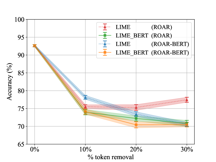
Figure 4: LIME${}_{\text{$\mathsf{BERT}$}}$ slightly, but consistently outperforms LIME when evaluated under either ROAR or ROAR${}_{\text{$\mathsf{BERT}$}}$. The each point in the $y$-axis shows the mean accuracy of five different classifiers. See more results supporting the same conclusion in Table E.

7 Discussion and Conclusion

We find in Sec. 5.3 that IM is highly insensitive to classifier’s changes because, by design, it always assigns near-zero attribution to highly-predictable words $x_{i}$ regardless of their true importance to a target classifier. A solution may be to leave such $x_{i}$ token out of the marginalization (Eq. 3), i.e. only marginalizing over the other tokens suggested by BERT. However, these other replacement tokens altogether have a sum likelihood of 0. That is, replacing token $x_{i}$ by zero-probability tokens (i.e. truly implausible) would effectively generate OOD text, which, in turn is not desired Hase et al. (2021).

Our results in Sec. 6.2 suggests that IM might be more useful at the phrase level Jin et al. (2020) instead of word level as deleting a set of contiguous words has a larger effect to the classifier predictions.

In sum, for the first time, we find that the popular idea of harnessing BERT to generate realistic counterfactuals Hase et al. (2021); Harbecke and Alt (2020); Kim et al. (2020) does not actually improve upon a simple LOO${}_{\text{$\mathsf{empty}$}}$ in practice as an LOO${}_{\text{$\mathsf{empty}$}}$ counterfactual only has a single word deleted. In contrast, we observe more expected benefits of this technique in improving methods like LIME that has counterfactuals that are extremely syntactically erroneous when multiple words are often deleted.

Acknowledgments

We thank Michael Alcorn, Qi Li, and Peijie Chen for helpful feedback on the early results. We also thank the anonymous reviewers for their detailed and constructive criticisms that helped us improve the manuscript. AN is supported by the National Science Foundation (grant 1850117; 2145767) and donations from Adobe Research and the NaphCare Charitable Foundation.

Appendix

Appendix A IM${}_{\text{$\mathsf{}$}}$ explanations have smaller attribution magnitude per token and lower word coverage

To further understand the impact of the fact that BERT tends to not change a to-remove token (Sec. B), here, we quantify the magnitude of attribution given by IM${}_{\text{$\mathsf{}$}}$ and its coverage of important words in an example.

Smaller attribution magnitude

Across three datasets, the average absolute values of attribution scores (which are $\in[-1,1])$ of IM${}_{\text{$\mathsf{}$}}$ are not higher than that of LOO${}_{\text{$\mathsf{empty}$}}$ (Table A1). Especially in MultiRC, IM${}_{\text{$\mathsf{}$}}$ average attribution magnitude is 4.5$\times$ lower than that of LOO${}_{\text{$\mathsf{empty}$}}$ (0.02 vs 0.09).

Method	SST	e-SNLI	MultiRC
LOO${}_{\text{$\mathsf{empty}$}}$	0.22 $\pm$ 0.27	0.15 $\pm$ 0.24	0.09 $\pm$ 0.09
IM${}_{\text{$\mathsf{}$}}$	0.17 $\pm$ 0.27	0.15 $\pm$ 0.27	0.02 $\pm$ 0.09

Table A1: The average absolute value of attribution scores per token of LOO${}_{\text{$\mathsf{empty}$}}$ is consistently higher than that of IM${}_{\text{$\mathsf{}$}}$.

Lower word coverage

We define coverage as the average number of highlighted tokens per example (e.g. Fig. 1) after binarizing a heatmap at the method’s optimal threshold.

The coverage of LOO${}_{\text{$\mathsf{empty}$}}$ is much higher than that of IM${}_{\text{$\mathsf{}$}}$ on SST (40% vs 30%) and MultiRC examples (27% vs 6%), which is consistent with the higher recall of LOO${}_{\text{$\mathsf{empty}$}}$ (Table A2; a vs. b). For e-SNLI, although IM${}_{\text{$\mathsf{}$}}$ has higher coverage than LOO${}_{\text{$\mathsf{empty}$}}$ (14% vs. 10%), the coverage of LOO${}_{\text{$\mathsf{empty}$}}$ is closer to the human coverage (9%). That is, IM${}_{\text{$\mathsf{}$}}$ assigns high attribution incorrectly to many words, resulting in a substantially lower precision than LOO${}_{\text{$\mathsf{empty}$}}$, according to e-SNLI L3 annotations (Table 5.1b; 0.3814 vs. 0.4687).

Explanations	SST	e-SNLI		MultiRC
generated by		L2	L3
(a) LOO${}_{\text{$\mathsf{empty}$}}$	40%	19%	10%	27%
(b) IM${}_{\text{$\mathsf{}$}}$	30%	21%	14%	6%
(c) Human	37%	18%	9%	16%
# tokens per example	20	24		299

Table A2: Compared to IM${}_{\text{$\mathsf{}$}}$, the coverage of LOO${}_{\text{$\mathsf{empty}$}}$ is closer to the coverage of human explanations.

In sum, chaining our results together, we found BERT to often replace a token $x_{i}$ by an exact-match with a high likelihood (Sec. B), which sets a low empirical upper-bound on attribution values of IM${}_{\text{$\mathsf{}$}}$, causing IM${}_{\text{$\mathsf{}$}}$ explanations to have smaller attribution magnitude. As the result, after binarization, fewer tokens remain highlighted in IM${}_{\text{$\mathsf{}$}}$ binary maps (e.g. Fig. 3).

Appendix B By design, IM always assigns near-zero attribution to high-likelihood words regardless of classifiers

We observe that IM${}_{\text{$\mathsf{}$}}$ scores a substantially lower recall compared to LOO${}_{\text{$\mathsf{empty}$}}$ (e.g. 0.0630 vs. 0.2876; Table 5.1d). That is, IM${}_{\text{$\mathsf{}$}}$ tends to incorrectly assign too small of attribution to important tokens. Here, we test whether this low-recall issue is because BERT is highly accurate at predicting a single missing word from the remaining text and therefore assigns a high likelihood to such words in Eq. 3, causing low IM attribution in Eq. 2.

Experiment

For each example in all three datasets, we replaced a single word by BERT’s top-1 highest-likelihood token and measured its likelihood and whether the replacement is the same as the original word.

Results

Across SST, e-SNLI, and MultiRC, the top-1 BERT token matches exactly the original word $\sim$49, 60, 65% of the time, respectively (Table A3a). This increasing trend of exact-match frequency (from SST, e-SNLI $\to$ MultiRC) is consistent with the example length in these three datasets, which is understandable as a word tends to be more predictable given a longer context. Among the tokens that human annotators label “important”, this exact-match frequency is similarly high (Table A3b). Importantly, the average likelihood score of a top-1 exact-match token is high, $\sim$0.81–0.86 (Table A3c). See Fig. 1 & Figs. A6–A11 for qualitative examples.

% exact-match (uncased)	SST	e-SNLI	MultiRC
(a) over all tokens	48.94	59.43	64.78
(b) over human highlights	41.25	42.74	68.55
(c) Top-1 word’s likelihood	0.8229	0.8146	0.8556

Table A3: Top-1 likelihood scores (c) are the mean likelihood given by BERT for the top-1 predicted words that exactly match the original words (a).

Our findings are aligned with IM${}_{\text{$\mathsf{}$}}$’s low recall. That is, if BERT fills in an exact-match $\tilde{x}_{i}$ for an original word $x_{i}$, the prediction difference for this replacement $\tilde{x}_{i}$ will be 0 in Eq. 4. Furthermore, a high likelihood of $\sim$0.81 for $\tilde{x}_{i}$ sets an empirical upper-bound of 0.19 for the attribution of the word $x_{i}$, which explains the insensitivity of IM to classifier randomization (Fig. 1; IM₁ to IM₃).

The analysis here is also consistent with our additional findings that IM attribution tends to be smaller than that of LOO${}_{\text{$\mathsf{empty}$}}$ and therefore leads to heatmaps of lower coverage of the words labeled “important” by humans (see Sec. A).

Appendix C Train BERT as masked language model on SST-2 to help filling in missing words

Integrating pre-trained BERT into LIME${}_{\text{$\mathsf{}$}}$ helps improve LIME explanations under two ROAR metrics (Sec. 6). However, the pre-trained BERT might be suboptimal for the cloze task on SST-2 sentences as it was pre-trained on Wikipedia and BookCorpus. Therefore, here, we take the pre-trained BERT, and finetune it on SST-2 training set using the masked language modeling objective. That is, we aim to test whether having a more specialized BERT would improve LIME results even further.

Training details

We follow the hyperparameters by Huggingface (2020) and use Adam optimizer Kingma and Ba (2015) with a learning rate of 0.00005, $\beta_{1}$ = 0.9, $\beta_{2}$ = 0.999, $\epsilon=10^{-8}$, a batch size of 8, max sequence length of 512 and the ratio of tokens to mask of 0.15. We finetune the pre-trained BERT on SST-2 Socher et al. (2013a) train set and select the best model using the dev set.

Results

On the SST-2 test set of 1,821 examples that contain 35,025 tokens in total, the cross-entropy loss of pre-trained BERT and BERT-SST2 are 3.50 $\pm$ 4.58 and 3.29 $\pm$ 4.40, respectively. That is, our BERT finetuned on SST-2 is better than pre-trained BERT at predicting missing words in SST-2 sentences.

Appendix D Comparison between original and modified version of Input Marginalization

We follow Kim et al. (2020) to reproduce results of the original Input Marginalization (IM) (Table A4a–b). To reduce the time complexity of Input Marginalization, we propose a modified version (IM-top10) by only marginalizing over the top-10 tokens sampled from BERT rather than using all tokens of likelihood $\geq$ a threshold $\sigma=10^{-5}$. We find that IM-top10 has comparable performance to that of the original IM (0.4732 vs. 0.4783; Table A4c). Our IM-top10 quantitative results are also close to the original numbers reported in Kim et al. (2020) (0.4922 vs. 0.4972; Table A4).

Metrics $\downarrow$	a. IM${}_{\text{$\mathsf{}$}}$ (reported in	b. IM${}_{\text{$\mathsf{}$}}$	c. IM${}_{\text{$\mathsf{}$}}$-top10
	Kim et al. (2020))	(Our reproduction)
Deletion	n/a	0.4783	0.4732
Deletion${}_{\text{$\mathsf{BERT}$}}$	0.4972	0.4824	0.4922

Table A4: The approximation in of IM-top10 compared to the original IM under two metrics on SST-2 task. Both metrics measure AUC (lower is better).

We also find high qualitative similarity between heatmaps produced by two versions: IM vs. IM-top10 (Figs. A1–5). The average Pearson correlation score across the SST-2 8720-example test set is fairly high ($\rho=0.7224$). Thus, we use IM-top10 for all experiments in this paper.

SST-2 example.  Groundtruth: “positive” &  Prediction: “positive” (Confidence: 0.9996)
IM	among	the	year	’s	most	intriguing	explorations	of	alientation	.
	1.815	0.0118	0.54158	0.22394	1.03458	5.03105	1.94109	1.53783	-0.31367	-0.0026
IM modified	among	the	year	’s	most	intriguing	explorations	of	alientation	.
	2.64685	0.03574	0.34608	0.51827	1.61421	5.74711	4.16886	2.30276	-0.35139	0.01431

Figure A1: Color map: negative -1, neutral 0, positive +1. Attribution maps derived from both versions of IM have a high Pearson correlation $\rho=0.988$.

SST-2 example.  Groundtruth: “positive” &  Prediction: “positive” (Confidence: 0.9994)
IM	a	solid	examination	of	the	male	midlife	crisis	.
	1.07654	6.16288	2.91817	-0.01502	0.14328	-0.40143	0.1654	1.29851	1.2264
IM modified	a	solid	examination	of	the	male	midlife	crisis	.
	1.83532	5.85144	2.89864	0.00083	0.02024	-0.11491	0.06725	1.11138	0.05947

Figure A2: Color map: negative -1, neutral 0, positive +1. Attribution maps derived from both versions of IM have a high Pearson correlation $\rho=0.917$.

SST-2 example.  Groundtruth: “negative” &  Prediction: “positive” (Confidence: 0.9868)
IM	rarely	has	leukemia	looked	so	shimmering	and	benign	.
	6.62645	0.98643	-2.15698	-0.16744	0.59491	8.38053	3.50372	0.15773	0.05112
IM modified	rarely	has	leukemia	looked	so	shimmering	and	benign	.
	3.11005	0.58616	-3.29759	-0.20848	0.3003	8.72728	3.81542	0.26226	0.04914

Figure A3: Color map: negative -1, neutral 0, positive +1. Attribution maps derived from both versions of IM have a high Pearson correlation $\rho=0.983$.

SST-2 example.  Groundtruth: “negative” &  Prediction: “negative” (Confidence: 0.9950)
IM	unfortunately	,	it	’s	not	silly	fun	unless	you	enjoy	really	bad	movies	.
	0.97455	-0.00063	-0.00634	-0.15033	0.81403	-1.31111	0.76075	-0.03599	-0.00042	-0.22804	0.27508	1.36045	0.58812	-0.00371
IM modified	unfortunately	,	it	’s	not	silly	fun	unless	you	enjoy	really	bad	movies	.
	1.6679	-0.00071	-0.00764	-0.35265	0.35085	-1.66804	-0.0029	0.37561	0.00036	-0.46997	0.35344	2.41716	0.78194	-0.00525

Figure A4: Color map: negative -1, neutral 0, positive +1. Attribution maps derived from both versions of IM have a high Pearson correlation $\rho=0.802$.

SST-2 example.  Groundtruth: “positive” &  Prediction: “negative” (Confidence: 0.7999)
IM	intriguing	documentary	which	is	emotionally	diluted	by	focusing	on	the	story	’s	least	interesting	subject	.
	-7.28604	-2.3813	-4.68492	-0.11221	0.40301	8.17448	1.71521	0.06288	0.00117	0.06125	-0.64145	1.74269	9.00071	1.50607	-0.22335	-0.15134
IM modified	intriguing	documentary	which	is	emotionally	diluted	by	focusing	on	the	story	’s	least	interesting	subject	.
	-3.96954	-1.1229	-2.38742	0.27984	4.07982	11.69405	0.68146	0.88004	-0.00308	0.04509	-0.43266	2.63444	9.97514	2.32102	-0.43297	0.03175

Figure A5: Color map: negative -1, neutral 0, positive +1. Attribution maps derived from both versions of IM have a high Pearson correlation $\rho=0.950$.

Appendix E Sanity check result

Criteria	Method	SST-2	e-SNLI
(a) % tokens changing sign	LOO${}_{\text{$\mathsf{empty}$}}$	71.41 $\pm$ 17.12	56.07 $\pm$ 21.82
	IM${}_{\text{$\mathsf{}$}}$	62.27 $\pm$ 17.75	49.57 $\pm$ 20.35
(b) Average absolute of differences	LOO${}_{\text{$\mathsf{empty}$}}$	0.46 $\pm$ 0.18	0.26 $\pm$ 0.14
	IM${}_{\text{$\mathsf{}$}}$	0.31 $\pm$ 0.12	0.16 $\pm$ 0.12

Table A5: The percentage (%) of token (a) whose attribution scores change signs and (b) the average of absolute differences in attribution magnitude after classifier randomization (higher is better). IM is consistently more insensitive than LOO${}_{\text{$\mathsf{empty}$}}$ in both SST-2 and e-SNLI.

lccc|ccc|ccc Accuracy $\downarrow$ ROAR ROAR${}_{\text{$\mathsf{BERT}$}}$ ROAR${}_{\text{$\mathsf{BERT\_SST2}$}}$
Method 10% 20% 30% 10% 20% 30% 10% 20% 30%
(a) LIME${}_{\text{$\mathsf{}$}}$ 75.51 $\pm$ 0.55 75.30 $\pm$ 0.80 77.45 $\pm$ 0.70 78.14 $\pm$ 0.54 73.44 $\pm$ 0.65 70.57 $\pm$ 0.56 78.83 $\pm$ 1.28 74.47 $\pm$ 0.67 72.18 $\pm$ 1.02
(b) LIME${}_{\text{$\mathsf{BERT}$}}$ 73.99 $\pm$ 0.74 72.22 $\pm$ 0.73 70.82 $\pm$ 0.86 74.13 $\pm$ 0.72 70.44 $\pm$ 0.86 70.48 $\pm$ 0.63 75.78 $\pm$ 0.22 71.33 $\pm$ 1.04 68.76 $\pm$ 0.79
(c) LIME${}_{\text{$\mathsf{BERT\_SST2}$}}$ 74.15 $\pm$ 1.26 70.85 $\pm$ 0.89 70.48 $\pm$ 0.98 76.19 $\pm$ 0.91 69.77 $\pm$ 0.46 67.61 $\pm$ 0.53 76.08 $\pm$ 0.46 70.92 $\pm$ 0.64 71.08 $\pm$ 0.34

Table A6: Dev-set mean accuracy (%) of 5 models trained on the new SST-2 examples where $N$% of highest-attribution words per example are removed (i.e. ROAR), replaced via BERT (i.e. ROAR${}_{\text{$\mathsf{BERT}$}}$) or BERT finetuned on SST-2 to fill in a [MASK] token (i.e. ROAR${}_{\text{$\mathsf{BERT\_SST2}$}}$). The original accuracy when no tokens are removed (i.e. $N=0$%) is 92.62 $\pm$ 0.30. On average, under three metrics, LIME${}_{\text{$\mathsf{BERT}$}}$ (b) and LIME${}_{\text{$\mathsf{BERT\_SST2}$}}$ (c) are better, i.e. lower mean accuracy, than LIME${}_{\text{$\mathsf{}$}}$ (a).

SST example.  Groundtruth: “positive”
S	may not have generated many sparks , but with his affection for Astoria and its people he has given his tale a warm glow .
S1	may not have generated many sparks , but with his affection for Astoria and its people he has given his tale a warm glow .
	0.9494  he             0.9105  given          0.9632  a
	0.0103  it                0.0285  lent              0.0270  its
	0.0066  ,                 0.0143  gave             0.0033  another

Figure A6: BERT${}_{\text{$\mathsf{}$}}$ often correctly predicts the masked tokens (denoted in red, green, blue rectangles) and assigns a high likelihood to the tokens that are labeled important by humans in the SST “positive” example. In each panel, we show the top-3 tokens suggested by BERT and their associated likelihoods.

SST example.  Groundtruth: “negative”
S	Villeneuve spends too much time wallowing in Bibi ’s generic angst ( there are a lot of shots of her gazing out windows ) .
S1	Villeneuve spends too much time wallowing in Bibi ’s generic angst ( there are a lot of shots of her gazing out windows ) .
	0.9987  much        0.9976  time          0.9675  in
	0.0011  little           0.0005  money        0.0066  with
	0.0001  some          0.0003  space          0.0062  on

Figure A7: BERT${}_{\text{$\mathsf{}$}}$ often correctly predicts the masked tokens (denoted in red, green, blue rectangles) and assigns a high likelihood to the tokens that are labeled important by humans in the SST “negative” example. In each panel, we show the top-3 tokens suggested by BERT and their associated likelihoods.

e-SNLI example.  Groundtruth: “entailment”
P	The two farmers are working on a piece of John Deere equipment .
H	John Deere equipment is being worked on by two farmers
P${}_{\text{1}}$	The two farmers are working on a piece of John Deere equipment
H${}_{\text{1}}$	John Deere equipment is being worked on by two farmers
	0.9995  john      0.9877  equipment    0.9711  john
	0.0000  johnny    0.0057  machinery      0.0243  the
	0.0000  henry      0.0024  hardware        0.0005  a

Figure A8: BERT${}_{\text{$\mathsf{}$}}$ often correctly predicts the masked tokens (denoted in red, green, blue rectangles) and assigns a high likelihood to the tokens that are labeled important by humans in the e-SNLI “entailment” example which contains a pair of premise (P) and hypothesis (H). In each panel, we show the top-3 tokens suggested by BERT and their associated likelihoods.

e-SNLI example.  Groundtruth: “neutral”
P	A man uses a projector to give a presentation .
H	A man is giving a presentation in front of a large crowd .
P${}_{\text{1}}$	A man uses a projector to give a presentation .
H${}_{\text{1}}$	A man is giving a presentation in front of a large crowd .
	1.0000  front         0.9999  of       0.9993  a
	0.0000  view           0.0000  to        0.0005  the
	0.0000  presence    0.0000  with    0.0001  another

Figure A9: BERT${}_{\text{$\mathsf{}$}}$ often correctly predicts the masked tokens (denoted in red, green, blue rectangles) and assigns a high likelihood to the tokens that are labeled important by humans in the e-SNLI “neutral” example which contains a pair of premise (P) and hypothesis (H). In each panel, we show the top-3 tokens suggested by BERT and their associated likelihoods.

MultiRC example.  Groundtruth & Prediction: “True” (confidence: 0.98)
P	What causes a change in motion ? The application of a force . Any time an object changes motion , a force has been applied . In what ways can this happen ? Force can cause an object at rest to start moving . Forces can cause objects to speed up or slow down . Forces can cause a moving object to stop . Forces can also cause a change in direction . In short , forces cause changes in motion . The moving object may change its speed , its direction , or both . We know that changes in motion require a force . We know that the size of the force determines the change in motion . How much an objects motion changes when a force is applied depends on two things . It depends on the strength of the force . It also depends on the objects mass . Think about some simple tasks you may regularly do . You may pick up a baseball . This requires only a very small force .
Q	What factors cause changes in motion of a moving object ?
A	The object ’s speed , direction , or both speed and direction
P${}_{\text{1}}$	What causes a change in motion ? The application of a force . Any time an object changes motion , a force has been applied . In what ways can this happen ? Force can cause an object at rest to start moving . Forces can cause objects to speed up or slow down . Forces can cause a moving object to stop . Forces can also cause a change in direction . In short , forces cause changes in motion . The moving object may change its speed , its direction , or both . We know that changes in motion require a force . We know that the size of the force determines the change in motion . How much an objects motion changes when a force is applied depends on two things . It depends on the strength of the force . It also depends on the objects mass . Think about some simple tasks you may regularly do . You may pick up a baseball . This requires only a very small force .
	0.9927  moving         0.9891  change       0.9995  or
	0.0023  moved            0.0033  alter             0.0004  and
	0.0016  stationary       0.0018  affect           0.0000  etc
Q${}_{\text{1}}$	John Deere equipment is being worked on by two farmers
A${}_{\text{1}}$	The object ’s speed , direction , or both speed and direction

Figure A10: BERT${}_{\text{$\mathsf{}$}}$ often correctly predicts the masked tokens (denoted in red, green, blue rectangles) and assigns a high likelihood to the tokens that are labeled important by humans in the MultiRC “True” example which contains a triplet of paragraph (P), question (Q) and answer (A). In each panel, we show the top-3 tokens suggested by BERT and their associated likelihoods.

MultiRC example.  Groundtruth & Prediction: “False” (confidence: 0.74)
P	There have been many organisms that have lived in Earths past . Only a tiny number of them became fossils . Still , scientists learn a lot from fossils . Fossils are our best clues about the history of life on Earth . Fossils provide evidence about life on Earth . They tell us that life on Earth has changed over time . Fossils in younger rocks look like animals and plants that are living today . Fossils in older rocks are less like living organisms . Fossils can tell us about where the organism lived . Was it land or marine ? Fossils can even tell us if the water was shallow or deep . Fossils can even provide clues to ancient climates .
Q	What are three things scientists learn from fossils ?
A	Who lived in prehistoric times
P${}_{\text{1}}$	There have been many organisms that have lived in Earths past . Only a tiny number of them became fossils . Still , scientists learn a lot from fossils . Fossils are our best clues about the history of life on Earth . Fossils provide evidence about life on Earth . They tell us that life on Earth has changed over time . Fossils in younger rocks look like animals and plants that are living today . Fossils in older rocks are less like living organisms . Fossils can tell us about where the organism lived . Was it land or marine ? Fossils can even tell us if the water was shallow or deep . Fossils can even provide clues to ancient climates .
	0.9984  life          0.9982  earth       0.9980  time
	0.0004  living       0.0007  mars         0.0007  millennia
	0.0002  things       0.0002  land         0.0003  history
Q${}_{\text{1}}$	What are three things scientists learn from fossils ?
A${}_{\text{1}}$	Who lived in prehistoric times

Figure A11: BERT${}_{\text{$\mathsf{}$}}$ often correctly predicts the masked tokens (denoted in red, green, blue rectangles) and assigns a high likelihood to the tokens that are labeled important by humans in the MultiRC “False” example which contains a triplet of paragraph (P), question (Q) and answer (A). In each panel, we show the top-3 tokens suggested by BERT and their associated likelihoods.

SST example.  Groundtruth & Prediction: “negative” (confidence: 1.00)
S	For starters , the story is just too slim .
S${}_{\text{IM}}$	For starters , the story is just too slim .
	IoU: 0.33, precision: 0.50, recall: 0.50
S${}_{\text{LOO}}$	For starters , the story is just too slim .
	IoU: 0.75, precision: 1.00, recall: 0.75

Figure A12: The set of explanatory words given by LOO${}_{\text{$\mathsf{empty}$}}$ covers 75% of human highlights with higher precision and IoU in the SST “negative” example while there are a half of tokens highlighted by IM${}_{\text{$\mathsf{}$}}$ are in correlation with human explanations.

e-SNLI example.  Groundtruth & Prediction: “contradiction” (confidence: 1.00)
P	Two men are cooking food together on the corner of the street .
H	The two men are running in a race .
P${}_{\text{IM}}$	Two men are cooking food together on the corner of the street .
H${}_{\text{IM}}$	The two men are running in a race .
	IoU: 0.25, precision: 0.33, recall: 0.50
P${}_{\text{LOO}}$	Two men are cooking food together on the corner of the street .
H${}_{\text{LOO}}$	The two men are running in a race .
	IoU: 0.50, precision: 0.50, recall: 1.00

Figure A13: The set of explanatory words given by LOO${}_{\text{$\mathsf{empty}$}}$ covers all highlights (higher precision and IoU) that are important to human in the e-SNLI “contradiction” example which contains a pair of premise (P) and hypothesis (H) while there are a half of tokens highlighted by IM${}_{\text{$\mathsf{}$}}$ are in correlation with human explanations.

e-SNLI example.  Groundtruth & Prediction: “neutral” (confidence: 1.00)
P	Woman in a dress standing in front of a line of a clothing line , with clothes hanging on the line .
H	Her dress is dark blue .
P${}_{\text{IM}}$	Woman in a dress standing in front of a line of a clothing line , with clothes hanging on the line .
H${}_{\text{IM}}$	Her dress is dark blue .
	IoU: 0.00, precision: 0.00, recall: 0.00
P${}_{\text{LOO}}$	Woman in a dress standing in front of a line of a clothing line , with clothes hanging on the line .
H${}_{\text{LOO}}$	Her dress is dark blue .
	IoU: 0.33, precision: 0.33, recall: 1.00

Figure A14: The set of explanatory words given by LOO${}_{\text{$\mathsf{empty}$}}$ covers all highlights (higher precision and IoU) that are important to human in the e-SNLI “neutral” example which contains a pair of premise (P) and hypothesis (H) while there are none tokens highlighted by IM${}_{\text{$\mathsf{}$}}$ are in correlation with human explanations.

MultiRC example.  Groundtruth & Prediction: “True” (confidence: 0.90)
P	There have been many organisms that have lived in Earths past . Only a tiny number of them became fossils . Still , scientists learn a lot from fossils . Fossils are our best clues about the history of life on Earth . Fossils provide evidence about life on Earth . They tell us that life on Earth has changed over time . Fossils in younger rocks look like animals and plants that are living today . Fossils in older rocks are less like living organisms . Fossils can tell us about where the organism lived . Was it land or marine ? Fossils can even tell us if the water was shallow or deep . Fossils can even provide clues to ancient climates .
Q	What happened to some organisms that lived in Earth ’s past ?
A	They became fossils . Others did not become fossils
P${}_{\text{IM}}$	There have been many organisms that have lived in Earths past . Only a tiny number of them became fossils . Still , scientists learn a lot from fossils . Fossils are our best clues about the history of life on Earth . Fossils provide evidence about life on Earth . They tell us that life on Earth has changed over time . Fossils in younger rocks look like animals and plants that are living today . Fossils in older rocks are less like living organisms . Fossils can tell us about where the organism lived . Was it land or marine ? Fossils can even tell us if the water was shallow or deep . Fossils can even provide clues to ancient climates .
Q${}_{\text{IM}}$	What happened to some organisms that lived in Earth ’s past ?
A${}_{\text{IM}}$	They became fossils . Others did not become fossils
	IoU: 0.16, precision: 0.50, recall: 0.19
P${}_{\text{LOO}}$	There have been many organisms that have lived in Earths past . Only a tiny number of them became fossils . Still , scientists learn a lot from fossils . Fossils are our best clues about the history of life on Earth . Fossils provide evidence about life on Earth . They tell us that life on Earth has changed over time . Fossils in younger rocks look like animals and plants that are living today . Fossils in older rocks are less like living organisms . Fossils can tell us about where the organism lived . Was it land or marine ? Fossils can even tell us if the water was shallow or deep . Fossils can even provide clues to ancient climates .
Q${}_{\text{LOO}}$	What happened to some organisms that lived in Earth ’s past ?
A${}_{\text{LOO}}$	They became fossils . Others did not become fossils
	IoU: 0.56, precision: 0.57, recall: 0.95

Figure A15: The set of explanatory words given by LOO${}_{\text{$\mathsf{empty}$}}$ covers 95% of human highlights with higher precision and IoU in the MultiRC “True” example which contains a triplet of paragraph (P), question (Q) and answer (A) while there are only few tokens given by IM${}_{\text{$\mathsf{}$}}$ are in correlation with human explanations.

MultiRC example.  Groundtruth & Prediction: “False” (confidence: 0.99)
P	There have been many organisms that have lived in Earths past . Only a tiny number of them became fossils . Still , scientists learn a lot from fossils . Fossils are our best clues about the history of life on Earth . Fossils provide evidence about life on Earth . They tell us that life on Earth has changed over time . Fossils in younger rocks look like animals and plants that are living today . Fossils in older rocks are less like living organisms . Fossils can tell us about where the organism lived . Was it land or marine ? Fossils can even tell us if the water was shallow or deep . Fossils can even provide clues to ancient climates .
Q	What is a major difference between younger fossils and older fossils ?
A	Older rocks are rougher and thicker than younger fossils
P${}_{\text{IM}}$	There have been many organisms that have lived in Earths past . Only a tiny number of them became fossils . Still , scientists learn a lot from fossils . Fossils are our best clues about the history of life on Earth . Fossils provide evidence about life on Earth . They tell us that life on Earth has changed over time . Fossils in younger rocks look like animals and plants that are living today . Fossils in older rocks are less like living organisms . Fossils can tell us about where the organism lived . Was it land or marine ? Fossils can even tell us if the water was shallow or deep . Fossils can even provide clues to ancient climates .
Q${}_{\text{IM}}$	What is a major difference between younger fossils and older fossils ?
A${}_{\text{IM}}$	Older rocks are rougher and thicker than younger fossils
	IoU: 0.06, precision: 0.18, recall: 0.08
P${}_{\text{LOO}}$	There have been many organisms that have lived in Earths past . Only a tiny number of them became fossils . Still , scientists learn a lot from fossils . Fossils are our best clues about the history of life on Earth . Fossils provide evidence about life on Earth . They tell us that life on Earth has changed over time . Fossils in younger rocks look like animals and plants that are living today . Fossils in older rocks are less like living organisms . Fossils can tell us about where the organism lived . Was it land or marine ? Fossils can even tell us if the water was shallow or deep . Fossils can even provide clues to ancient climates .
Q${}_{\text{LOO}}$	What is a major difference between younger fossils and older fossils ?
A${}_{\text{LOO}}$	Older rocks are rougher and thicker than younger fossils
	IoU: 0.22, precision: 0.25, recall: 0.67

Figure A16: The set of explanatory words given by LOO${}_{\text{$\mathsf{empty}$}}$ covers two thirds of human highlights with higher precision and IoU in the MultiRC “False” example which contains a triplet of paragraph (P), question (Q) and answer (A) while there are two tokens given by IM${}_{\text{$\mathsf{}$}}$ are in correlation with human explanations.

SST example.  Groundtruth & Prediction: “positive”
S	Enormously entertaining for moviegoers of any age .
S1	Enormously entertaining for moviegoers of any age .
S2	Enormously entertaining for moviegoers of any age .
S3	Enormously entertaining for moviegoers of any age .
S4	Enormously entertaining for moviegoers of any age .
S5	Enormously entertaining for moviegoers of any age .
S6	Enormously entertaining for moviegoers of any age .
S7	Enormously entertaining for moviegoers of any age .

Figure A17: When a word is removed, the predicted labels of all resulting sentences (S₁ to S₇) are still “positive” with a confidence score of 1.0.

e-SNLI example.  Groundtruth: “entailment”		Prediction
P	Two women having drinks and smoking cigarettes at the bar .	entailment (0.99)
H	Two women are at a bar .
P${}_{\text{1}}$	Two women having drinks and smoking cigarettes at the bar .	entailment (0.98)
H${}_{\text{1}}$	Two women are at a bar .
P${}_{\text{2}}$	Two women having drinks and smoking cigarettes at the bar .	neutral (0.93)
H${}_{\text{2}}$	Two women are at a bar .
P${}_{\text{3}}$	Two women having drinks and smoking cigarettes at the bar .	entailment (0.99)
H${}_{\text{3}}$	Two women are at a bar .
P${}_{\text{4}}$	Two women having drinks and smoking cigarettes at the bar .	entailment (0.99)
H${}_{\text{5}}$	Two women are at a bar .
P${}_{\text{5}}$	Two women having drinks and smoking cigarettes at the bar .	entailment (0.99)
H${}_{\text{5}}$	Two women are at a bar .
P${}_{\text{6}}$	Two women having drinks and smoking cigarettes at the bar .	entailment (0.99)
H${}_{\text{6}}$	Two women are at a bar .
P${}_{\text{7}}$	Two women having drinks and smoking cigarettes at the bar .	entailment (0.99)
H${}_{\text{7}}$	Two women are at a bar .
P${}_{\text{8}}$	Two women having drinks and smoking cigarettes at the bar .	entailment (0.98)
H${}_{\text{8}}$	Two women are at a bar .
P${}_{\text{9}}$	Two women having drinks and smoking cigarettes at the bar .	entailment (0.98)
H${}_{\text{9}}$	Two women are at a bar .
P${}_{\text{10}}$	Two women having drinks and smoking cigarettes at the bar .	entailment (0.97)
H${}_{\text{10}}$	Two women are at a bar .
P${}_{\text{11}}$	Two women having drinks and smoking cigarettes at the bar .	entailment (0.99)
H${}_{\text{11}}$	Two women are at a bar .
P${}_{\text{12}}$	Two women having drinks and smoking cigarettes at the bar .	entailment (0.99)
H${}_{\text{12}}$	Two women are at a bar .
P${}_{\text{13}}$	Two women having drinks and smoking cigarettes at the bar .	entailment (0.98)
H${}_{\text{13}}$	Two women are at a bar .
P${}_{\text{14}}$	Two women having drinks and smoking cigarettes at the bar .	entailment (0.99)
H${}_{\text{14}}$	Two women are at a bar .
P${}_{\text{15}}$	Two women having drinks and smoking cigarettes at the bar .	entailment (0.84)
H${}_{\text{15}}$	Two women are at a bar .
P${}_{\text{16}}$	Two women having drinks and smoking cigarettes at the bar .	entailment (0.97)
H${}_{\text{16}}$	Two women are at a bar .
P${}_{\text{17}}$	Two women having drinks and smoking cigarettes at the bar .	entailment (0.54)
H${}_{\text{17}}$	Two women are at a bar .
P${}_{\text{18}}$	Two women having drinks and smoking cigarettes at the bar .	entailment (0.95)
H${}_{\text{18}}$	Two women are at a bar .

Figure A18: The removal of each token in both premise and hypothesis in e-SNLI example which contains a pair of premise (P) and hypothesis (H) infrequently change the prediction. Specifically, only the example of (P₂, H₂) shifted its prediction to “neutral” while the remaining partially-removed examples do not change their original prediction with high confidence score in parentheses.

References

- Adebayo et al. (2018) Julius Adebayo, Justin Gilmer, Michael Muelly, Ian Goodfellow, Moritz Hardt, and Been Kim. 2018. Sanity checks for saliency maps. In Advances in Neural Information Processing Systems, volume 31. Curran Associates, Inc.
- Agarwal and Nguyen (2020) Chirag Agarwal and Anh Nguyen. 2020. Explaining image classifiers by removing input features using generative models. In Proceedings of the Asian Conference on Computer Vision.
- Arras et al. (2017) Leila Arras, Grégoire Montavon, Klaus-Robert Müller, and Wojciech Samek. 2017. Explaining recurrent neural network predictions in sentiment analysis. EMNLP 2017, page 159.
- Bansal et al. (2020) Naman Bansal, Chirag Agarwal, and Anh Nguyen. 2020. Sam: The sensitivity of attribution methods to hyperparameters. In Proceedings of the IEEE/CVF Conference on Computer Vision and Pattern Recognition, pages 8673–8683.
- Bowman et al. (2015) Samuel R. Bowman, Gabor Angeli, Christopher Potts, and Christopher D. Manning. 2015. A large annotated corpus for learning natural language inference. In Proceedings of the 2015 Conference on Empirical Methods in Natural Language Processing (EMNLP). Association for Computational Linguistics.
- Camburu et al. (2018) Oana-Maria Camburu, Tim Rocktäschel, Thomas Lukasiewicz, and Phil Blunsom. 2018. e-snli: Natural language inference with natural language explanations. In Advances in Neural Information Processing Systems, volume 31. Curran Associates, Inc.
- Chang et al. (2019) Chun-Hao Chang, Elliot Creager, Anna Goldenberg, and David Duvenaud. 2019. Explaining image classifiers by counterfactual generation. In International Conference on Learning Representations.
- Covert et al. (2020) Ian Covert, Scott Lundberg, and Su-In Lee. 2020. Feature removal is a unifying principle for model explanation methods. arXiv preprint arXiv:2011.03623.
- Dabkowski and Gal (2017) Piotr Dabkowski and Yarin Gal. 2017. Real time image saliency for black box classifiers. In Advances in Neural Information Processing Systems, pages 6967–6976.
- Devlin et al. (2019) Jacob Devlin, Ming-Wei Chang, Kenton Lee, and Kristina Toutanova. 2019. Bert: Pre-training of deep bidirectional transformers for language understanding. In Proceedings of the 2019 Conference of the North American Chapter of the Association for Computational Linguistics: Human Language Technologies, Volume 1 (Long and Short Papers), pages 4171–4186.
- DeYoung et al. (2020) Jay DeYoung, Sarthak Jain, Nazneen Fatema Rajani, Eric Lehman, Caiming Xiong, Richard Socher, and Byron C. Wallace. 2020. ERASER: A benchmark to evaluate rationalized NLP models. In Proceedings of the 58th Annual Meeting of the Association for Computational Linguistics, pages 4443–4458, Online. Association for Computational Linguistics.
- Fong et al. (2019) Ruth Fong, Mandela Patrick, and Andrea Vedaldi. 2019. Understanding deep networks via extremal perturbations and smooth masks. In Proceedings of the IEEE/CVF International Conference on Computer Vision, pages 2950–2958.
- Goyal et al. (2019) Yash Goyal, Amir Feder, Uri Shalit, and Been Kim. 2019. Explaining classifiers with causal concept effect (cace). arXiv preprint arXiv:1907.07165.
- Harbecke and Alt (2020) David Harbecke and Christoph Alt. 2020. Considering likelihood in NLP classification explanations with occlusion and language modeling. In Proceedings of the 58th Annual Meeting of the Association for Computational Linguistics: Student Research Workshop, pages 111–117, Online. Association for Computational Linguistics.
- Hase et al. (2021) Peter Hase, Harry Xie, and Mohit Bansal. 2021. The out-of-distribution problem in explainability and search methods for feature importance explanations. Advances in Neural Information Processing Systems, 34.
- Hooker et al. (2019) Sara Hooker, Dumitru Erhan, Pieter-Jan Kindermans, and Been Kim. 2019. A benchmark for interpretability methods in deep neural networks. In Advances in Neural Information Processing Systems, volume 32. Curran Associates, Inc.
- Huggingface (2020) Huggingface. 2020. Pretrained models — transformers 3.3.0 documentation. https://huggingface.co/transformers/pretrained_models.html. (Accessed on 09/30/2020).
- Jin et al. (2020) Xisen Jin, Zhongyu Wei, Junyi Du, Xiangyang Xue, and Xiang Ren. 2020. Towards hierarchical importance attribution: Explaining compositional semantics for neural sequence models. In International Conference on Learning Representations.
- Khashabi et al. (2018) Daniel Khashabi, Snigdha Chaturvedi, Michael Roth, Shyam Upadhyay, and Dan Roth. 2018. Looking beyond the surface: A challenge set for reading comprehension over multiple sentences. In Proceedings of the 2018 Conference of the North American Chapter of the Association for Computational Linguistics: Human Language Technologies, Volume 1 (Long Papers), pages 252–262, New Orleans, Louisiana. Association for Computational Linguistics.
- Kim et al. (2020) Siwon Kim, Jihun Yi, Eunji Kim, and Sungroh Yoon. 2020. Interpretation of NLP models through input marginalization. In Proceedings of the 2020 Conference on Empirical Methods in Natural Language Processing (EMNLP), pages 3154–3167, Online. Association for Computational Linguistics.
- Kingma and Ba (2015) Diederik P Kingma and Jimmy Ba. 2015. Adam: A method for stochastic optimization. Published as a conference paper at the 3rd International Conference for Learning Representations, San Diego.
- Lai and Tan (2019) Vivian Lai and Chenhao Tan. 2019. On human predictions with explanations and predictions of machine learning models: A case study on deception detection. In Proceedings of the conference on fairness, accountability, and transparency, pages 29–38.
- Li et al. (2016) Jiwei Li, Will Monroe, and Dan Jurafsky. 2016. Understanding neural networks through representation erasure. arXiv preprint arXiv:1612.08220.
- Liu and Avci (2019) Frederick Liu and Besim Avci. 2019. Incorporating priors with feature attribution on text classification. In Proceedings of the 57th Annual Meeting of the Association for Computational Linguistics, pages 6274–6283, Florence, Italy. Association for Computational Linguistics.
- Lundberg and Lee (2017) Scott M Lundberg and Su-In Lee. 2017. A unified approach to interpreting model predictions. In Advances in neural information processing systems, pages 4765–4774.
- Pearl (2009) Judea Pearl. 2009. Causality. Cambridge university press.
- Ribeiro (2021) Ribeiro. 2021. marcotcr/lime: Lime: Explaining the predictions of any machine learning classifier. https://github.com/marcotcr/lime. (Accessed on 05/17/2021).
- Ribeiro et al. (2016) Marco Tulio Ribeiro, Sameer Singh, and Carlos Guestrin. 2016. Why should i trust you?: Explaining the predictions of any classifier. In Proceedings of the 22nd ACM SIGKDD international conference on knowledge discovery and data mining, pages 1135–1144. ACM.
- Robnik-Šikonja and Kononenko (2008) Marko Robnik-Šikonja and Igor Kononenko. 2008. Explaining classifications for individual instances. IEEE Transactions on Knowledge and Data Engineering, 20(5):589–600.
- Socher et al. (2013a) Richard Socher, Alex Perelygin, Jean Wu, Jason Chuang, Christopher D. Manning, Andrew Ng, and Christopher Potts. 2013a. Recursive deep models for semantic compositionality over a sentiment treebank. In Proceedings of the 2013 Conference on Empirical Methods in Natural Language Processing, pages 1631–1642, Seattle, Washington, USA. Association for Computational Linguistics.
- Socher et al. (2013b) Richard Socher, Alex Perelygin, Jean Wu, Jason Chuang, Christopher D Manning, Andrew Y Ng, and Christopher Potts. 2013b. Recursive deep models for semantic compositionality over a sentiment treebank. In Proceedings of the 2013 conference on empirical methods in natural language processing, pages 1631–1642.
- Wiegreffe and Marasović (2021) Sarah Wiegreffe and Ana Marasović. 2021. Teach me to explain: A review of datasets for explainable nlp. arXiv preprint arXiv:2102.12060.
- Zeiler and Fergus (2014) Matthew D Zeiler and Rob Fergus. 2014. Visualizing and understanding convolutional networks. In European conference on computer vision, pages 818–833. Springer.
- Zhang et al. (2019) Yujia Zhang, Kuangyan Song, Yiming Sun, Sarah Tan, and Madeleine Udell. 2019. " why should you trust my explanation?" understanding uncertainty in lime explanations. arXiv preprint arXiv:1904.12991.
- Zhou et al. (2016) Bolei Zhou, Aditya Khosla, Agata Lapedriza, Aude Oliva, and Antonio Torralba. 2016. Learning deep features for discriminative localization. In Proceedings of the IEEE conference on computer vision and pattern recognition, pages 2921–2929.