Azade Farshad*azade.farshad@tum.de1 \addauthorSabrina Musatian*sabrina.musatian@tum.de1 \addauthorHelisa Dhamohelisa.dhamo@tum.de1 \addauthorNassir Navabnassir.navab@tum.de1
Technical University of Munich
Munich, Germany
Meta Image Generation from Scene Graphs
Supplementary Material: MIGS: Meta Image Generation from Scene Graphs
1 Experiment On Memorization
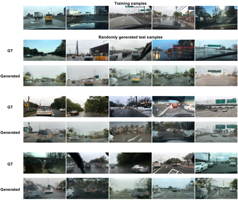
In Figure 1 we show training samples for a 5-shot training task and generated images from the test set of the same task, along with the corresponding ground truth images. As it can be seen in the figure, the generated images are different from the 5 training samples in terms of e.g. car colors or shapes. It should be noted that the model has generated cars with different colours than the ones it was exposed to by the training samples. The diversity of the generated images is shown to be better than the original sg2im model given the Precision and Recall metric in Table 1, and FID and KID metrics. In the testing phase, for each task consisting of different images and their corresponding scene graphs, 5 different images (in the case of 5-shot) are sampled and used for fine-tuning the model. Then other images (with different scene graphs) from the same task with similar attributes are sampled. Their scene graph is used to generate images and the generated images are compared to the ground truth ones.
2 Additional Quantitative Results
In this section we provide quantitative evaluation of our method compared to baseline using precision () and recall () metrics [30] for BDD (Table 1) and AG(Table 2) datasets.
| Method | Decoder | F_8 | F_1/8 | F_8 | F_1/8 | F_8 | F_1/8 |
|---|---|---|---|---|---|---|---|
| 160-shot | 10-shot | 5-shot | |||||
| SG2Im | CRN | 0.101 | 0.135 | 0.063 | 0.131 | 0.06 | 0.057 |
| MIGS(Ours) | CRN | 0.06 | 0.176 | 0.052 | 0.123 | 0.05 | 0.06 |
| SG2Im | SPADE | 0.486 | 0.612 | 0.462 | 0.45 | 0.329 | 0.438 |
| MIGS(Ours) | SPADE | 0.7 | 0.86 | 0.79 | 0.854 | 0.74 | 0.823 |
On both datasets MIGS + SPADE outperforms the corresponding baseline by almost twice. Such supremacy means that the images generated with the meta-learning approach are more realistically looking (precision) and cover more modes of the underlying real data distribution (recall). The results obtained for MIGS + CRN are comparable to the ones of the baseline.
| Method | Decoder | F_8 | F_1/8 |
|---|---|---|---|
| SG2Im | CRN | 0.217 | 0.116 |
| MIGS(Ours) | CRN | 0.167 | 0.09 |
| SG2Im | SPADE | 0.59 | 0.31 |
| MIGS(Ours) | SPADE | 0.6 | 0.5 |
3 Extra Qualitative Results
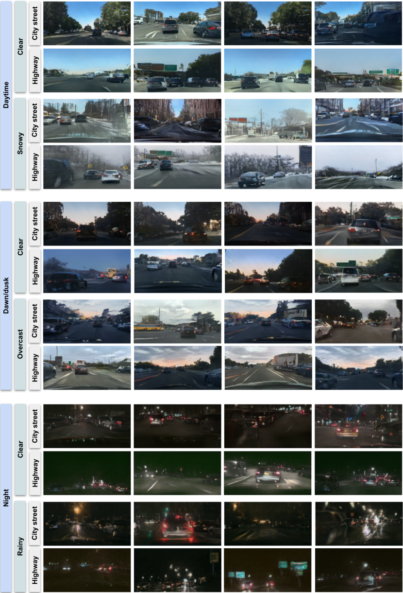
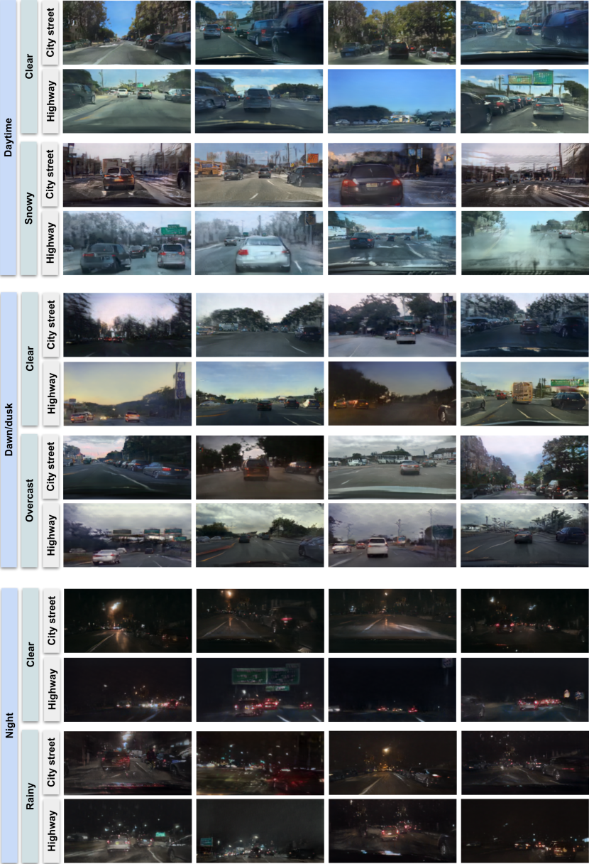
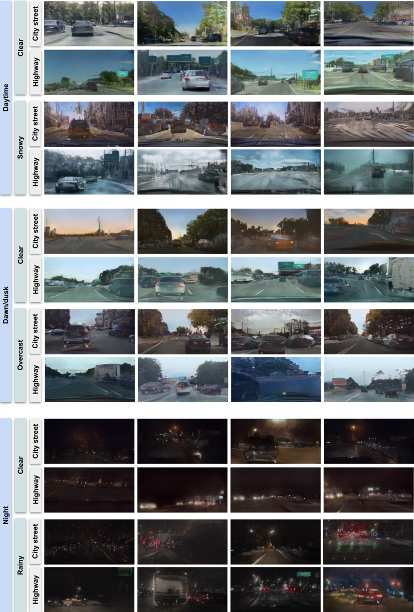
Here we demonstrate additional qualitative results of MIGS on the BDD dataset in 160-shot learning (Figure 2), 10-shot learning (Figure 3) and 5-shot learning (Figure 4). We observe that the model generates compelling results for a diverse set of tasks. All images were generated using MIGS with SPADE generator. Both 160 and 10-shot learning models are able to generate various sets of images even within one particular task. The results of these two models are comparable in quality and both are able to depict such fine-grained details as clouds in the overcast task or glares from the rain on the road. 5-shot learning can produce realistically looking images for many tasks, but struggles with reproducing significantly differently looking images within one particular task. It also cannot generate as many details as can be seen in 160 and 10-shot learning models. This behavior is not surprising, as the model sees only a very limited amount of training images, so it might be impossible to depict such diversity from this set.
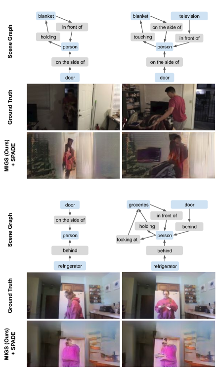
Additionally, we provide more qualitative results on AG dataset (Figure 5) to demonstrate that our method can correctly capture the semantic relationships between the objects, specified by the scene graph in different scenarios.
4 User study
For the perceptual study, images were generated randomly for three different scene attributes (daytime, dawn/dusk, night) with examples of each. Each image was seen by workers. In each example, the user receives four images in random order – representing our four methods in study – and is asked to provide a ranking among them. In addition, we provide a checkbox for each image, through which the user can indicate whether a certain attribute is met.
5 Architecture details
CRN
The CRN variant of the decoder network contains cascaded refinement blocks, which have namely 1024, 512, 256, 128 and 64 channels. Every block consists of two convolutions, each followed by batch norm and leaky ReLU. The output of each module is concatenated with the initial input to the CRN, re-scaled to the feature resolution.
SPADE
The SPADE decoder consists of residual blocks, which have namely 1024, 512, 256, 128 and 64 channels. Instead of the semantic map in the original implementation, here we use the layout to modulate the layer activations in each block. The global discriminator contains two scales.
GCN
The GCN network consists of layers. Each layer processes triplets of subject - predicate - object embeddings, which are obtained by feeding each semantic label in an embedding layer. Every layer consists of three steps. First, the propagation layer (a two-layer MLP) receives the concatenated triplet feature and results in a 128 channels output. Second, the aggregation layer computes the average of features that correspond to a certain node. Third, the update layer applies a final processing of each node feature via another two-layer MLP. Both MLPs above have a hidden layer of 512 channels. The input embeddings of the objects and predicates have dimensions each. The last layer of the GCN returns the node features (128 channels), binary masks () and bounding box prediction by applying a two-layer MLP with a hidden layer size of .