L-2 Regularized maximum likelihood for $\beta$-model in large and sparse networks

Abstract

The $\beta$-model is a powerful tool for modeling network generation driven by degree heterogeneity. Its simple yet expressive nature particularly well-suits large and sparse networks, where many network models become infeasible due to computational challenge and observation scarcity. However, existing estimation algorithms for $\beta$-model do not scale up; and theoretical understandings remain limited to dense networks. This paper brings several significant improvements to the method and theory of $\beta$-model to address urgent needs of practical applications. Our contributions include: 1. method: we propose a new $\ell_{2}$ penalized MLE scheme; we design a novel fast algorithm that can comfortably handle sparse networks of millions of nodes, much faster and more memory-parsimonious than all existing algorithms; 2. theory: we present new error bounds on $\beta$-models under much weaker assumptions than best known results in literature; we also establish new lower-bounds and new asymptotic normality results; under proper parameter sparsity assumptions, we show the first local rate-optimality result in $\ell_{2}$ norm; distinct from existing literature, our results cover both small and large regularization scenarios and reveal their distinct asymptotic dependency structures; 3. application: we apply our method to large COVID-19 network data sets and discover meaningful results.

Keywords— Network analysis; $\beta$-model; Sparse networks; Big data; Regularization.

1 Introduction

1.1 The $\beta$-model: formulation, motivating data examples and previous work

The $\beta$-model (Chatterjee et al., 2011), is a heterogeneous exponential random graph model (ERGM) with the degree sequence as the exclusively sufficient statistic. It is a popular model for networks mainly driven by degree heterogeneity. Under this model, an undirected and binary network of $n$ nodes, represented by its adjacency matrix $A=(A_{i,j})_{1\leq\{i,j\}\leq n}\in\{0,1\}^{n\times n}$, is generated by

$$\mathbb{P}(A_{i,j}=1)=\dfrac{e^{\beta_{i}^{*}+\beta_{j}^{*}}}{1+e^{\beta_{i}^{*}+\beta_{j}^{*}}},\quad A_{i,j}=A_{j,i},\quad 1\leq i<j\leq n,$$ (1)

where $\beta^{*}=(\beta_{1}^{*},\ldots,\beta_{n}^{*})$ denotes the vector of true model parameters, and edges $\{A_{i,j}:i<j\}$ are mutually independent. Set $A_{i,i}\equiv 0$ for all $i$. The negative log-likelihood function is

$$\mathcal{L}({\beta})= \sum_{1\leq i<j\leq n}\log\big{(}1+e^{\beta_{i}+\beta_{j}}\big{)}-\sum_{i=1}^{n}\beta_{i}d_{i}.$$ (2)

where $d_{1},\ldots,d_{n}$ are observed node degrees: $d_{i}=\sum_{j\neq i}A_{i,j}$.

The $\beta$-model is a simple, yet expressive tool for describing degree heterogeneity, a feature of paramount importance in many networks (Babai et al., 1980; Fienberg, 2012). Here we briefly describe two motivating data sets. First, (Elmer et al., 2020) collected social networks between a group of Swiss students before and during COVID-19 lockdown. For privacy protection, they only released node degrees instead of adjacency matrix. The $\beta$-model can be fitted to this data while most other popular models which need adjacency matrix cannot be applied. The second example is a massive COVID-19 knowledge graph (Steenwinckel et al., 2020). It contains $n\approx 10^{7}$ non-isolated nodes with just $2.1\times 10^{7}$ million edges. The $\beta$-model shows its unique advantages of high speed and memory parsimony in handling this data. We will present detailed analyses of these data sets in Section 6.

Since its birth, the $\beta$-model has attracted a lot of research interest. The early works Holland and Leinhardt (1981); Chatterjee et al. (2011); Park and Newman (2004); Rinaldo et al. (2013); Hillar and Wibisono (2013) studied basic model properties and established existence, consistency and asymptotic normality of the vanilla MLE. Chen and Olvera-Cravioto (2013); Yan et al. (2016, 2019); Stein and Leng (2021) extended the model for directed and bipartite networks. Karwa and Slavković (2016) studied differential privacy in $\beta$-model. Graham (2017); Su et al. (2018); Gao (2020); Yan et al. (2019); Stein and Leng (2020, 2021) incorporated nodal or edge-wise covariates. Wahlström et al. (2017) established the Cramer-Rao bound with repeated network observations. Mukherjee et al. (2018) studied a different variant of $\beta$-model for sparse network with a known sparsity parameter.

1.2 Regularized $\beta$-models

The most relevant to the topic of this paper are the recent pioneering works Chen et al. (2021) and Stein and Leng (2020). They introduced regularization into the $\beta$-model literature. The main idea is that a simplified parameter space would help address sparse networks. Chen et al. (2021) proposed the following sparse $\beta$-model (S$\beta$M). Suppose there exists a set ${\cal S}\subseteq[1:n]$, called active set, such that

$$\beta_{i}^{*}=\begin{cases}-\gamma/2\log n+\mu^{\dagger}/2,&\textrm{ if }i\notin{\cal S},\\ (\alpha-\gamma/2)\log n+\mu^{\dagger}/2+\beta_{i}^{\dagger},&\textrm{ if }i\in{\cal S},\end{cases}$$ (3)

where $\alpha$ and $\gamma$ are positive constants, and $\max\{|\mu^{\dagger}|,|\beta_{i}^{\dagger}|\}=o(\log n)$. They assume that $\gamma$ and $\alpha$ are known and show that one can consistently estimate the $o(\log n)$ parts of the parameters $(\mu^{\dagger},\beta_{i}^{\dagger})$ using a constrained MLE with user-specified upper bound on the size of the estimated ${\cal S}$. Their approach can be viewed as an $\ell_{0}$-regularized MLE. Stein and Leng (2020) proposed an $\ell_{1}$-regularized MLE. The model assumption of Stein and Leng (2020) can be roughly understood as a relaxed version of (3), where we have $\alpha_{i}$ for each $i\in{\cal S}$ instead of a uniform $\alpha$. Their method can be reformulated as

$$\arg\min_{\beta,\beta_{0}}{\cal L}_{\lambda;\beta_{0}}(\beta)= ~{}{\cal L}(\beta)+\lambda\big{\|}\beta-\beta_{0}\cdot\mathbbm{1}\big{\|}_{1},$$ (4)

where $\mathbbm{1}$ is an all-one vector and $\lambda$ is a tuning parameter. Remark that our choice of $\lambda$ is different from theirs. This is an $\ell_{1}$-regularized MLE approach.

In this paper, we adopt a symbol system based on the original formulation of the $\beta$-model (1) and propose an $\ell_{2}$-regularized MLE, as follows

$$\arg\min_{\beta}{\cal L}_{\lambda}(\beta)= ~{}{\cal L}(\beta)+\frac{\lambda}{2}\big{\|}\beta-\bar{\beta}\cdot\mathbbm{1}\big{\|}_{2}^{2},$$ (5)

where notice that we use $\bar{\beta}=n^{-1}\sum_{i=1}^{n}\beta_{i}$ instead of $\beta_{0}$, since the optimal $\beta_{0}$ equals $\bar{\beta}$. Our $\ell_{2}$ penalty is a softer version of $\ell_{0}$ (Chen et al., 2021) and $\ell_{1}$ (Stein and Leng, 2020, 2021) penalties, thus is more flexible for modeling networks where $\beta^{*}$ may not be $\ell_{0}$ sparse. In this paper, we shall propose a fast algorithm for solving (5), establish accompanying theory, and conduct comprehensive simulation studies and data applications.

1.3 Our contributions

The main theme of our paper is an $\ell_{2}$-regularized MLE. Therefore, we will focus more on comparing with Chen et al. (2021) and Stein and Leng (2020) in this part. Table 1 highlights the main differences and improvements of our work over Chen et al. (2021) and Stein and Leng (2020) and provides pointers to corresponding sections in this paper.

Chen et al. (2021) Stein and Leng (2020) Our paper Discussed in Penalty $l_{0}$ $l_{1}$ $l_{2}$ Section 1.2 Model (3) (3) with $\alpha_{i}$ for each $i$, $\mu^{\dagger}=\beta_{i}^{\dagger}=0$ (1) Section 1.2 Parameter constraint Known $\gamma$ and $\alpha$; $\alpha>0$ $\alpha_{i}>0$ None Section 1.2 MLE existence Not always guaranteed Yes Yes Section 2.1 Computation cost $O(n^{3})$ per iteration $O(n^{3})$ per iteration $O(n\cdot\bar{d})$ + ($O(m^{2})$ per iteration) Section 2.2 Need network sparsity $\gg n^{-1/2}$ $\gg n^{-1/6}$ $\gg n^{-1}$ Section 3.1 Finite-sample error bound No Yes Yes Section 3.1 Sparsistency Yes Yes Yes Section 3.1 Lower bound result No No Yes Section 3.2 Local rate-optimality No No Yes Section 3.2 Asymptotic normality Fixed-dimensional Fixed-dimensional High-dimensional Section 3.3 Data-driven tuning of $\lambda$ Yes Yes Yes Section 4 Empirical scalability $n\approx 10^{3}$ $n\approx 10^{3}$ $n\approx 10^{7}$ Sections 5 and 6

Table 1: Comparison table between Chen et al. (2021), Stein and Leng (2020) and our paper.

Now, we summarize our main contributions.

1. Weaker model assumptions and simple MLE existence guarantee. Both Chen et al. (2021) and Stein and Leng (2020) assume that most nodes have a common (or nearly common) low expected degree, whereas a few nodes in the active set ${\cal S}$ have higher degrees. Chen et al. (2021) further assumes that those high-degree nodes also have similar expected degrees. Our paper makes no such assumptions. Our method and accompanying theory can also be applied to $\beta$-models that do not have such “parameter sparsity” structure, which Chen et al. (2021) and Stein and Leng (2020) are not provably valid for.

   In the past, Rinaldo et al. (2013) devoted much effort into finding a complicated sufficient and necessary condition for MLE existence. The same treatment was inherited by Chen et al. (2021). We show that a simple “$\lambda>0$” is sufficient to guarantee the existence of our $\ell_{2}$-regularization MLE, similar to Stein and Leng (2020).

2. Proposing a very fast new algorithm for large and sparse networks. Computation has long been a challenge for $\beta$-models. To out best knowledge, all existing works resort to either some general optimizer Chen et al. (2021) or use GLM packages Yan et al. (2019); Stein and Leng (2020) for parameter estimation, which typically cannot scale up to networks with $10^{4}$ nodes (see Table 1) and do not take advantage of network sparsity. In this paper, we propose a novel algorithms that fully exploits the structure of the $\beta$-model and particularly specialize for handling large and sparse networks. For example, our new algorithm only takes a few minutes on a personal computer to fit a $\beta$-model to the Steenwinckel et al. (2020) data that contains $O(10^{7})$ nodes.

3. Theory is the most highlighted part of this paper. We believe our work represents a giant leap in the theoretical understandings of $\beta$-models. Our main theoretical contributions include:

   1. Handling much sparser networks. Existing $\beta$-model literature (Chatterjee et al., 2011; Yan and Xu, 2013; Yan et al., 2016) typically requires that $\rho_{n}=\binom{n}{2}^{-1}\sum_{1\leq i<j\leq n}A_{i,j}\gtrsim{\rm Polynomial}(\log^{-1}n)$ for consistency, where $\rho_{n}$ is the network density. Apparently, Chen et al. (2021) can handle network sparsity down to $\rho_{n}\gg n^{-1/2}$. However, their theory is built upon an unrealistic assumption of knowing the true values of $\gamma$ and $\alpha$ in their model, while in view of Stein and Leng (2020), estimating unknown $\gamma$ and $\alpha$ is the really hard part of the problem. Stein and Leng (2020) does not make such assumption, but they can only handle a network sparsity of $\rho_{n}\gg n^{-1/6}$. In sharp contrast, our method is guaranteed to be consistent for much sparser networks. For example, if all edges probabilities are on the same asymptotic order, we only need $\rho_{n}\gg n^{-1}$ to guarantee $\ell_{\infty}$ consistency. For more details, see Section 3.1.

   2. Finite-sample upper bounds and provably sparsistent post-estimation variable selection. Our theory provides finite-sample $\ell_{\infty}$ and $\ell_{2}$ error bounds. The $\ell_{\infty}$ error bound enables a post-estimation variable selection algorithm (see Corollary 1) that allows us to consistently estimate ${\cal S}$ under the settings of either Chen et al. (2021) and Stein and Leng (2020). Our method not only computes much faster, but also requires much weaker assumption on the size of ${\cal S}$. Chen et al. (2021) assumes $|{\cal S}|\ll n$ and Stein and Leng (2020) assumes $|{\cal S}|\lesssim n^{1/2}$ in order to guarantee estimation consistency. We do not need such assumption and our theory, applied to Chen et al. (2021)’s model, only requires ${\cal S}\leq Cn$ for any constant $C\in(0,1/2)$.

   3. Finite-sample lower bound results and local rate-optimality. Existing $\beta$-model literature presents very little understanding of lower bound results. We establish the first set of lower bound results for $\beta$-model with one single observation of the network. As a highlighted contribution, we find that our estimator is locally rate-optimal in $\ell_{2}$ norm for estimating a $\beta$-model with true parameter $\beta^{*}$ being “$\beta$-sparse” (in the sense of Chen et al. (2021)). This is the first estimation optimality result in $\beta$-model literature. We also established the local and non-local lower bounds in different $\ell_{p}$ norms, which are a little different from upper bounds, up to a logarithmic factor.

   4. High-dimensional asymptotic normality and characterization of estimator’s behavior under heavy penalty. All existing asymptotic normality results for $\beta$-models are fixed-dimensional. We present the first high-dimensional asymptotic normality result. Moreover, our theory reveals an interesting contrast in the asymptotic covariance structures under light and heavy penalties. When $\lambda$ is small, the estimator’s elements tend to be independent; and when $\lambda$ is large, they become nearly perfectly dependent. This is verified by our simulation. Our paper provides the first characterization of the behavior of the regularized estimator with a large $\lambda$ in the $\beta$-model literature. Our proof techniques in this part is original and very different from other $\beta$-model papers.

4. Our other contributions include the follows. We develop a data-driven AIC-type criterion for automatically selecting the tuning parameter $\lambda$. Simulation results verify its effectiveness. In the discussion section, we also present empirical studies to gauge the feasibility of a popular idea on testing goodness-of-fit of network models applied to the $\beta$-model.

1.4 Notation

We inherit the asymptotic notion $O(\cdot)$, $o(\cdot)$, $\lesssim$ and $\asymp$ from standard calculus. Let $\mathbbm{1}=(1,\ldots,1)^{T}$. For any vector $u\in\mathbb{R}^{n\times 1}$ and matrix $U\in\mathbb{R}^{n\times n}$, define matrices $V(u)$ and $V(U)$ as follows: for all $1\leq\{i\neq j\}\leq n$, define $\{V(u)\}_{i,j}=e^{u_{i}+u_{j}}/(1+e^{u_{i}+u_{j}})^{2}$ and $\{V(U)\}_{i,j}=e^{U_{i,j}}/(1+e^{U_{i,j}})$; and for all $1\leq i\leq n$, define $V_{i,i}=\sum_{1\leq j\leq n,j\neq i}V_{i,j}$ for $V=V(u)$ or $V=V(U)$. For any vector $x$, inherit the standard notion of $\ell_{p}$ norms $\|x\|_{p}$ for $p=0,1,2,\infty$. For any matrix $J\in\mathbb{R}^{n\times n}$, define $\|J\|_{\infty}=\sup_{x\neq 0}\|Jx\|_{\infty}/\|x\|_{\infty}=\max_{1\leq i\leq n}\sum_{j=1}^{n}|J_{i,j}|$. Also inherit Frobenius norm $\|\cdot\|_{F}$ and spectral norm $\|\cdot\|_{\rm op}$ from standard matrix analysis. For two matrices $A_{1},A_{2}\in\mathbb{R}^{n\times n}$, write $A_{1}\geq A_{2}$ to denote element-wise comparison: $A_{1;i,j}\geq A_{2;i,j}$ for all $1\leq\{i,j\}\leq n$. Finally, we import two concepts of “sparsity” from Chen et al. (2021): network sparsity refers to Chen et al. (2021) $\rho_{n}=\sum_{1\leq i<j\leq n}\mathbb{E}[A_{i,j}]/\binom{n}{2}$, and $\beta$-sparsity means that most $\beta_{i}^{*}$’s share a common value.

2 Our method

In this section, we present the parameter estimation and the fast algorithm for our model. Statistical inference would require quantitative theoretical study, therefore, we relegate them to Section 3.

2.1 Parameter estimation

Recall our method from (5). Denote the gradient of ${\cal L}_{\lambda}(\beta)$ by $F(\beta)=\big{(}F_{1}(\beta),\ldots,F_{n}(\beta)\big{)}$. We have

$$F_{i}(\beta)= \dfrac{\partial{\cal L}_{\lambda}(\beta)}{\partial\beta_{i}}=\sum_{\begin{subarray}{c}1\leq j\leq n\\ j\neq i\end{subarray}}\dfrac{e^{\beta_{i}+\beta_{j}}}{1+e^{\beta_{i}+\beta_{j}}}-d_{i}+\lambda(\beta_{i}-\bar{\beta}),\quad 1\leq i\leq n.$$ (6)

We estimate the model parameters by solving the following equation set

$$F(\widehat{\beta}_{\lambda})=0.$$ (7)

There are two immediate questions regarding (7): the existence and the uniqueness of its solution. We first address the uniqueness of MLE, assuming its existence. It suffices to show the strict convexity of the $\ell_{2}$-regularized likelihood ${\cal L}_{\lambda}(\beta)$. Denote the Jacobian matrix of ${\cal L}_{\lambda}(\beta)$ by $F^{\prime}(\beta)$, we have

$$\{F^{\prime}(\beta)\}_{i,j}=\dfrac{\partial F_{i}}{\partial\beta_{j}}(\beta)= \dfrac{\partial F_{j}}{\partial\beta_{i}}(\beta)=\dfrac{e^{\beta_{i}+\beta_{j}}}{\big{(}1+e^{\beta_{i}+\beta_{j}}\big{)}^{2}}-\dfrac{\lambda}{n}, \textrm{ for }1\leq\{i\neq j\}\leq n,$$ (8)

$$\{F^{\prime}(\beta)\}_{i,i}=\dfrac{\partial F_{i}}{\partial\beta_{i}}(\beta)= \sum_{\begin{subarray}{c}1\leq j\leq n\\ j\neq i\end{subarray}}\dfrac{e^{\beta_{i}+\beta_{j}}}{\big{(}1+e^{\beta_{i}+\beta_{j}}\big{)}^{2}}+\dfrac{(n-1)\lambda}{n}, \textrm{ for }1\leq i\leq n.$$ (9)

For narration convenience, we define the projection matrices for the subspace spanned by $\mathbbm{1}$:

$${\cal P}=n^{-1}\mathbbm{1}\mathbbm{1}^{T},\quad{\cal P}_{\perp}=I-n^{-1}\mathbbm{1}\mathbbm{1}^{T}.$$ (10)

Using the notion $V(\beta)$ defined in Section 1.4, we rewrite the Jacobian matrix as

$$F^{\prime}(\beta)=V(\beta)+\lambda I-\frac{\lambda}{n}\mathbbm{1}\mathbbm{1}^{T}=V(\beta)+\lambda{\cal P}_{\perp}.$$ (11)

By Theorem 1.1 of Hillar et al. (2012), $V(\beta)$ is globally strictly positive definite; also, ${\cal P}_{\perp}$ is semi-positive definite. Therefore, ${\cal L}_{\lambda}(\beta)$ is strictly convex, thus the solution to (7) is unique.

Next, let us discuss existence. The MLE existence conditions for the vanilla $\beta$-model (1) and its $\ell_{0}$-regularized version (Chen et al., 2021) in existing literature assume that the degree vector $d$ is an interior point of $B$, where $B$ is solved from $d=B\cdot{\rm vec}(A)$ for vec$(A)$ being the vectorization of $A$, see Proposition 2.1 in Hillar and Wibisono (2013), Rinaldo et al. (2013) and Appendix B of Chen et al. (2021). Such conditions are complicated and infeasible to verify in practice. In sharp contrast, our proposed $\ell_{2}$-regularization provides a much cleaner guarantee of MLE existence.

Lemma 1

For any $\lambda>0$ and any $n$, there exists a finite $\widehat{\beta}_{\lambda}\in\mathbbm{R}^{n}$ such that $F(\widehat{\beta}_{\lambda})=0$.

The MLE existence is thus guaranteed by Lemma 1 and the global strict convexity of ${\cal L}_{\lambda}(\beta)$ that we showed earlier. For the rest of this paper, we may sometimes set “$\lambda=0$” for formula succinctness – readers may understand it as “setting $\lambda$ to be a small positive value”, in view of Lemma 1.

In the next subsection, we present our proposed fast algorithm to numerically solve (7).

2.2 Fast algorithm via dimensionality reduction by degree-indexing

The majority of existing $\beta$-model works (Yan et al., 2015, 2016; Chen et al., 2021; Stein and Leng, 2021) numerically estimate the parameters using generic GLM or optimization packages such as glmnet, which typically cost $O(n^{3})$ computation per iteration (see Section “Cost of Computation” in Amazon H2O (2021) and Equation (4.26) in Section 4.4.1 of Hastie et al. (2009)). Consequently, they cannot scale above $O(10^{3})$ nodes. Generic packages do not exploit the structure of the large and sparse but patterned design matrix under the $\beta$-model. Indeed, one can alternatively solve (7) by gradient descent or Newton’s method, but the $O(n^{2})$ per-iteration cost is still expensive.

Here, we present a novel algorithm that takes full advantage of (i) the structure of the $\beta$-model’s likelihood function; and (ii) the widely-observed sparsity of large networks. The idea of our method stems from the following monotonicity lemma.

Lemma 2

The MLE $\widehat{\beta}_{\lambda}$ (solution to (7)) satisfies that $\widehat{\beta}_{\lambda;i}=\widehat{\beta}_{\lambda;j}$ if and only if $d_{i}=d_{j}$, for any $1\leq i<j\leq n$, where $\widehat{\beta}_{\lambda;i}$ denotes the $i$th element of $\widehat{\beta}_{\lambda}$.

We clarify that the monotonicity phenomenon was first discovered not by us, but by Hillar and Wibisono (2013) (Proposition 2.4). The proof of Lemma 2 is a close variant of its counterparts in earlier literature Hillar and Wibisono (2013); Chen et al. (2021). However, Hillar and Wibisono (2013) did not connect their monotonicity lemma to computation; and Chen et al. (2021) used it exclusively for variable selection. In contrast, we are the first to realize that Lemma 2 can greatly reduce the dimensionality of parameter estimation, which leads to a giant leap in both speed and memory efficiency.

We now describe our algorithm. Let $d_{(1)}<d_{(2)}<\cdots<d_{(m)}$ be the sorted unique values of observed degrees, where $m=\big{|}\textrm{Unique}\big{(}\{d_{1},\ldots,d_{n}\}\big{)}\big{|}$. For each $k\in\{1,\ldots,m\}$, let ${\cal D}_{k}:=\{i_{1}^{(k)},\ldots,i_{n_{k}}^{(k)}\}\subseteq\{1,\ldots,n\}$ collect all those nodes whose degrees equal $d_{(k)}$, namely, $d_{i_{1}^{(k)}}=\cdots=d_{i_{n_{k}}^{(k)}}=d_{(k)};$ and $d_{j}\neq d_{(k)},$ for all $j\notin{\cal D}_{k}$. Define $n_{k}:=|{\cal D}_{k}|$. Then due to Lemma 2, in the MLE, all $\beta_{j}$’s with $j\in{\cal D}_{k}$ should be set to a common value, denoted by $\delta_{k}$. The objective function ${\cal L}_{\lambda}(\beta)$ can be “re-parameterized” into a function of degree-indexed parameters $\delta:=(\delta_{1},\ldots,\delta_{m})$, called $\widetilde{\cal L}_{\lambda}(\delta)$:

$$\widetilde{\cal L}_{\lambda}(\delta):={\cal L}_{\lambda}(\beta)= \sum_{1\leq k<\ell\leq m}n_{k}n_{\ell}\log\Big{(}1+e^{\delta_{k}+\delta_{\ell}}\Big{)}+\sum_{1\leq k\leq m}\dfrac{n_{k}(n_{k}-1)}{2}\log\Big{(}1+e^{2\delta_{k}}\Big{)}$$

$$-\sum_{k=1}^{m}n_{k}d_{(k)}\delta_{k}+\dfrac{\lambda}{2}\sum_{k=1}^{m}n_{k}(\delta_{k}-\widetilde{\delta})^{2},$$ (12)

where $\widetilde{\delta}:=n^{-1}\sum_{k=1}^{m}n_{k}\cdot\delta_{k}$ is the weighted average, conceptually analogous to $\bar{\beta}$ under the original parameterization. The gradient of $\widetilde{\cal L}_{\lambda}(\beta)$ is

$$G_{k}(\delta):= \dfrac{\partial\widetilde{\cal L}_{\lambda}(\beta)}{\partial\delta_{k}}=\sum_{\begin{subarray}{c}1\leq\ell\leq m\\ \ell\neq k\end{subarray}}n_{k}n_{\ell}\dfrac{e^{\delta_{k}+\delta_{\ell}}}{1+e^{\delta_{k}+\delta_{\ell}}}+n_{k}(n_{k}-1)\dfrac{e^{2\delta_{k}}}{1+e^{2\delta_{k}}}-n_{k}d_{(k)}+n_{k}(\delta_{k}-\widetilde{\delta})\lambda,$$ (13)

and its Jacobian matrix, denoted by $J$, is

$$J_{k\ell}(\delta)=\dfrac{\partial^{2}\widetilde{\cal L}_{\lambda}(\delta)}{\partial\delta_{k}\partial\delta_{\ell}}= ~{}n_{k}n_{\ell}\dfrac{e^{\delta_{k}+\delta_{\ell}}}{\big{(}1+e^{\delta_{k}+\delta_{\ell}}\big{)}^{2}}-\dfrac{n_{k}n_{\ell}}{n}\lambda,\quad\textrm{ for }1\leq\{k\neq\ell\}\leq m,$$ (14)

$$J_{kk}(\delta)=\dfrac{\partial^{2}\widetilde{\cal L}_{\lambda}(\delta)}{\partial\delta_{k}^{2}}= ~{}\sum_{\begin{subarray}{c}1\leq\ell\leq m\\ \ell\neq k\end{subarray}}n_{k}n_{\ell}\dfrac{e^{\delta_{k}+\delta_{\ell}}}{\big{(}1+e^{\delta_{k}+\delta_{\ell}}\big{)}^{2}}+2n_{k}(n_{k}-1)\dfrac{e^{2\delta_{k}}}{\big{(}1+e^{2\delta_{k}}\big{)}^{2}}$$

$$+n_{k}\Big{(}1-\dfrac{n_{k}}{n}\Big{)}\lambda,\quad\textrm{ for }1\leq k\leq m.$$ (15)

We do not need to separately study the existence and uniqueness of $\widehat{\delta}_{\lambda}:=\arg\min_{\delta}\widetilde{\cal L}_{\lambda}(\delta)$, because (1) minimizing $\widetilde{\cal L}_{\lambda}(\delta)$ is the same as minimizing ${\cal L}_{\lambda}(\beta)$ under the additional constraint introduced by Lemma 2; and (2) the optimal solution $\widehat{\beta}_{\lambda}$ to the unconstrained problem $\min_{\beta}{\cal L}_{\lambda}(\beta)$ exists, is unique (recall Section 2.1), and satisfies that constraint. Therefore, the $\widehat{\delta}_{\lambda}$, which corresponds to $\widehat{\beta}_{\lambda}$, would also be the unique optimal solution to $\min_{\delta}\widetilde{\cal L}_{\lambda}(\delta)$.

Our new algorithm is particularly effective in handling large and sparse networks, where the total number of different node degrees $m$ is much smaller than the network size $n$. Its computational complexity is bottle-necked by the first step: computing all node degrees, which would cost $O(\rho_{n}\cdot n^{2})$ time, where recall that $\rho_{n}$ represents network sparsity. Then each iteration in the gradient method would cost $O(m^{2})$. All these are much cheaper than the $O(n^{3})$ per-iteration cost in existing literature.

The data set Steenwinckel et al. (2020) provides a striking example of the scalability of our method. It contains $n\approx 1.3$ million nodes, but only $m=459$ different degrees. Many nodes share common low degrees, see Table 2. Our algorithm makes it feasible to run a Newton’s method on this network of seemingly prohibitive size.

Table 2: Frequencies of low degrees in the data set Steenwinckel et al. (2020), $n=1304155$.

Degree	1	2	3	4	5
Number of nodes with this degree	684003	132123	48126	24586	15189
Percentage of nodes, unit: %	52.45	10.13	3.69	0.19	0.12

We conclude this subsection by clarifying that the “re-parameterization” (12)–(15) is employed only for computation, namely, finding the MLE. Throughout the theoretical analysis in the next Section, we would always stick to the MLE $\widehat{\beta}_{\lambda}$ under the original parameterization.

3 Theory and theory-based statistical inference

Throughout this section, we assume the true parameters satisfy $\beta^{*}\in{\cal S}_{1}=[a_{1}^{*}\log n-M^{*},a_{2}^{*}\log n+M^{*}]^{n}$ for some constants $a_{1}^{*}<a_{2}^{*}$ and $M^{*}>0$. To better connect to existing $\beta$-model literature, we define the following shorthand.

Definition 1

For the true parameter value $\beta^{*}$, define

$$b_{n}=\max_{1\leq i<j\leq n} \dfrac{(1+e^{\beta_{i}^{*}+\beta_{j}^{*}})^{2}}{e^{\beta_{i}^{*}+\beta_{j}^{*}}},\quad c_{n}=\min_{1\leq i<j\leq n}\dfrac{(1+e^{\beta_{i}^{*}+\beta_{j}^{*}})^{2}}{e^{\beta_{i}^{*}+\beta_{j}^{*}}},$$

and $$~{}{\color[rgb]{0,0,0}q_{n}=\Bigg{\{}\max_{1\leq i\leq n}(n-1)^{-1}\sum_{\begin{subarray}{c}1\leq j\leq n\\ j\neq i\end{subarray}}\dfrac{e^{\beta_{i}^{*}+\beta_{j}^{*}}}{(1+e^{\beta_{i}^{*}+\beta_{j}^{*}})^{2}}\Bigg{\}}^{-1}}.$$ (16)

By definition, $b_{n}^{-1}$ and $c_{n}^{-1}$ are minimum and maximum edge probabilities, and $(n-1)q_{n}^{-1}$ is the maximum expected degree. Clearly, $b_{n}^{-1}\leq q_{n}^{-1}\leq c_{n}^{-1}$. In this paper, we do not discuss very dense networks where edges are nearly all 1’s, not only due to that most real-world networks are sparse, but also because we can model $\{1-A_{i,j}\}_{1\leq\{i,j\}\leq n}$ as a sparse network. Formally:

Assumption 1

Zero edges are not sparse, that is, $c_{n}^{-1}\leq 1-C_{0}$ for some constant $C_{0}\in(0,1)$.

To simplify the presentation of our main results, we make the following assumption for convenience.

Assumption 2

There exists at least four distinct nodes $i_{1},i_{2},j_{1},j_{2}\in[1:n]$, such that $\max\big{(}|\beta_{i_{1}}^{*}-a_{1}^{*}\log n|,|\beta_{i_{2}}^{*}-a_{1}^{*}\log n|,|\beta_{j_{1}}^{*}-a_{2}^{*}\log n|,|\beta_{j_{2}}^{*}-a_{2}^{*}\log n|\big{)}=O(1)$.

The sole purpose of Assumption 2 is to reduce the number of symbols in theorems and ease reading. It implies that $b_{n}\asymp\widetilde{b}_{n}$, where $\widetilde{b}_{n}\asymp\sup_{\beta_{1},\beta_{2}\in[a_{1}^{*}\log n+C_{1},a_{2}^{*}\log n+C_{2}]}(1+e^{\beta_{1}+\beta_{2}})^{2}/e^{\beta_{1}+\beta_{2}}$ for any constants $C_{1},C_{2}$, so that we will not need to set up a separate symbol $\widetilde{b}_{n}$ when presenting theoretical results, especially those places that may otherwise involve both $b_{n}$ and $\widetilde{b}_{n}$. The same goes for $c_{n}$.

3.1 Consistency and finite-sample error bounds

Following the convention of the $\beta$-model literature, we first present an $\ell_{\infty}$ bound.

Theorem 1

Define

$$\Gamma(n,~{} \beta^{*};\lambda):=\dfrac{\log^{1/2}n}{b_{n}^{-1}n}\cdot\dfrac{\lambda}{b_{n}^{-1}n+\lambda}+\dfrac{({\color[rgb]{0,0,0}q_{n}^{-1}}n\log n)^{1/2}+\|{\cal P}_{\perp}\beta^{*}\|_{\infty}\lambda}{b_{n}^{-1}n+\lambda}\cdot\Big{(}1+\dfrac{b_{n}}{{\color[rgb]{0,0,0}q_{n}}}\cdot\dfrac{\|{\cal P}_{\perp}\beta^{*}\|_{\infty}\lambda}{b_{n}^{-1}n+\lambda}\Big{)}.$$ (17)

Assume that

$$(b_{n}/{\color[rgb]{0,0,0}q_{n}})\cdot\Gamma(n,\beta^{*};\lambda){\color[rgb]{0,0,0}~{}\leq 1/20.}$$ (18)

Then our $\ell_{2}$-regularized MLE $\widehat{\beta}_{\lambda}$ satisfies

$$\mathbb{P}\Big{\{}\|\widehat{\beta}_{\lambda}-\beta^{*}\|_{\infty}\leq ~{}C_{1}\Gamma(n,\beta^{*};\lambda)\Big{\}}\geq 1-n^{-C_{2}}$$ (19)

for some constants $C_{1},C_{2}>0$, where $C_{1}$ depends on $C_{2}$.

Theorem 1 holds for all choices of $\lambda$, as long as (18) is satisfied. To better parse it, we discuss two representative choices of $\lambda$. First, we set $\lambda=O(1)$. Recall that our Lemma 1 guarantees the existence of MLE for any $\lambda>0$, so $\widehat{\beta}_{\lambda}$ is well-defined. Then the assumption (18) can be simplified to $(b_{n}^{4}/q_{n}^{3})\cdot n^{-1}\log n\to 0$, and the error bound becomes $\Gamma(n,\beta^{*};\lambda)\asymp\big{\{}(b_{n}^{2}/q_{n})\cdot n^{-1}\log n\big{\}}^{1/2}$. To further simplify, we can consider the set up of Chen et al. (2021), where $\beta_{i}^{*}=(-\gamma\log n+\mu^{\dagger})/2+\mathbbm{1}_{[i\in{\cal S}]}(\alpha\log n+\mathfrak{b}_{i}^{\dagger})$, where ${\cal S}\subset[1:n]$ is the “active set” satisfying $|{\cal S}|\ll n^{1-\alpha}$, and $\vee_{i=1}^{n}|\mathfrak{b}_{i}^{\dagger}|\vee|\mu^{\dagger}|\ll\log n$.

Now we compare our Theorem 1 with $\lambda=O(1)$ to Chen et al. (2021) and Stein and Leng (2020) and elaborate the improvement. Under the setting of Chen et al. (2021), our assumption (18) becomes $\gamma+3\alpha<1$. Now $\rho_{n}\asymp n^{-\gamma}$ represents network sparsity, this says that when $\beta_{i}^{*}$’s are sufficiently homogeneous, our Theorem 1 can handle networks as sparse as $\rho_{n}\gg n^{-1}$ – this is a widely-recognized minimal sparsity assumption across many different topics in network literature Bickel and Chen (2009); Zhao et al. (2012); Zhang and Xia (2022).

In contrast, Theorem 1 and Lemma 2 in Chen et al. (2021) not only assume knowing the true values of $\gamma$ and $\alpha$ (in fact, $\gamma$ is the bottle neck of estimation accuracy – compare the error rates of $\gamma$ and that of the individualism parameters in Theorem 1 of Stein and Leng (2020)), but they also additionally assume that $\rho_{n}\gg n^{-1/2}$. Stein and Leng (2020) makes a much stronger assumption that $\rho_{n}\gtrsim n^{-1/6}$. Therefore, our Theorem 1 significantly improves over these state-of-the-art results.

In general, our Theorem 1’s assumption demands a compromise between network sparsity and degree heterogeneity. This is understandable, since the presence of high degree discrepancy makes Jacobian matrix $F^{\prime}(\beta^{*})$ ill-conditioned thus deteriorates the local convexity of the likelihood around $\beta^{*}$, making parameter estimation harder. In some special settings, such as Chen et al. (2021), where there are essentially only two kinds of nodes: hub nodes with $\beta_{i}\approx(\alpha-\gamma/2)\log n$ and peripheral nodes with $\beta_{j}\approx-\gamma/2\cdot\log n$, ad-hoc strategies such as estimating high- and low-degree nodes separately may effectively patch up this issue, but in general, high heterogeneity remains a major challenge for $\beta$-model studies.

Next, we briefly discuss the behavior of $\widehat{\beta}_{\lambda}$ when $\lambda\to\infty$. Theorem 1 of Stein and Leng (2020) shows an error bound that grows quadratically with $\lambda$ in terms of the $L_{1}$ norm. In contrast, our error bound in terms of the $L_{\infty}$ norm gives $\lim_{\lambda\to\infty}\Gamma(n,\beta^{*};\lambda)=b_{n}\log^{1/2}/n+\|{\cal P}_{\perp}\beta^{*}\|_{\infty}\cdot\big{\{}1+(b_{n}/q_{n}\cdot\|{\cal P}_{\perp}\beta^{*}\|_{\infty})\big{\}}$ if $\lambda\gg n/b_{n}$. The first term approximately matches the error bound in fitting an Erdos-Renyi model, agreeing with the intuitions that large $\lambda$ penalizes parameters to an Erdos-Renyi graph. The second error term is due to regularization.

Based on Theorem 1, when Assumption (18) is satisfied, our method can identify node $i$’s whose true $\beta_{i}^{*}$ is significantly different from the majority. In the spirit of Chen et al. (2021) and Chen et al. (2021), this can be called as “sparsistency” or variable selection consistency (Li et al., 2015). In practice, to carry out this post-estimation thresholding, we need to estimate $q_{n}$ and $b_{n}$. To simplify narration, in this part of the paper, we are working under the $\beta$-model with the $\beta$-sparsity from Chen et al. (2021). The following corollary provides a theoretically guaranteed algorithm to carry out a post-estimation variable selection for our $\ell_{2}$-regularized MLE.

Corollary 1 (Sparsistency of post-estimation thresholding)

Consider the setting of Chen et al. (2021) in (3). Then under the assumptions of our Theorem 1 (with $\lambda=O(1)$) and the assumption from Chen et al. (2021) that $|{\cal S}|\ll n^{1-\alpha}$, when $\alpha>0$, the following algorithm:

• Step 1: Run our $\ell_{2}$-regularized MLE with a $\lambda=O(1)$ to produce $\widehat{\beta}_{\lambda}$;

• Step 2: Take the subset of nodes whose degrees are the middle $\zeta_{0}$ proportion. Here $\zeta_{0}$ can be any fixed number in $(0,1)$, such as $\zeta_{0}=50\%$. Let $A_{\zeta_{0}}$ denote the $(\zeta_{0}n)\times(\zeta_{0}n)$ submatrix induced by the selected nodes. Let $\bar{A}_{\zeta_{0}}$ denote $\binom{\zeta_{0}n}{2}^{-1}\sum_{1\leq i<j\leq n}(A_{\zeta_{0}})_{i,j}$. Set $\widehat{b}_{n}=\bar{A}_{\zeta_{0}}(1-\bar{A}_{\zeta_{0}})$;

• Step 3: Output $\widehat{\cal S}=\big{\{}j:|\widehat{\beta}_{\lambda;j}-\log\{\bar{A}_{\zeta_{0}}/(1-\bar{A}_{\zeta_{0}})\}|>\{\widehat{q}_{n}^{-1}\log n/(\widehat{b}_{n}^{-2}n)\}^{1/2}\big{\}}$;

outputs an estimator $\widehat{\cal S}$ that enjoys the sparsistency guarantee: $\mathbb{P}(\widehat{\cal S}={\cal S})\to 1$.

Remark 1

Now we compare our Corollary 1 to the counterparts in Chen et al. (2021) and Stein and Leng (2020). The main advantage of our approach compared to Chen et al. (2021) is computational speed. Chen et al. (2021) treats the estimation of ${\cal S}$ as a model selection problem; they therefore fit the model many times at different sparsity levels. In sharp contrast, our new theoretical results reveals a new and different understanding that in fact, the MLE with a small amount of regularization can achieve sparsistency, without going through model selection, thus saving a lot of computation. Notice that our argument here is not based on our fast degree-indexed estimation algorithm, because we expect our dimension reduction technique can also be applied to Chen et al. (2021), though it still needs some adaptation to carefully handle ties in observed node degrees. We notice that Stein and Leng (2020) did not discuss estimation of ${\cal S}$, possibly because they studied a more general $\beta$-model where the $\beta_{i}^{*}$’s for those $i\in{\cal S}$ can have substantive differences from each other. We believe that some separation conditions such as those we assumed in Corollary 1 (“$\alpha>0$”) and the “min-$\beta$ condition” in Chen et al. (2021) would be necessary to discuss sparsistency in the setting of Stein and Leng (2020).

Next we present our $\ell_{2}$ error bound.

Theorem 2

Set $\lambda>0$. There exists constants $C_{1},C_{2}>0$, where $C_{1}$ depends on $C_{2}$, such that with probability at least $1-n^{-C_{1}}$, we have

1. Set $\lambda=O(1)$. Suppose we perform a constrained MLE with $\widehat{\beta}_{\lambda}\in[a_{1}\log n-M,a_{2}\log n+M]^{n}$ for some $M>0$ and $a_{1},a_{2}$ satisfying $a_{1}\leq a_{1}^{*}\leq a_{2}^{*}\leq a_{2}$. Then we have

   $$n^{-1/2}\cdot\|\widehat{\beta}_{\lambda}-\beta^{*}\|_{2}\leq ~{}C_{2}\big{\{}(b_{n}^{\prime})^{2}/q_{n}\cdot n^{-1}\log n\big{\}}^{1/2},$$ (20)

   where $b_{n}^{\prime}:=\max\{e^{2a_{1}}/(1+e^{2a_{1}})^{2},e^{2a_{2}}/(1+e^{2a_{2}})^{2}\}$.

2. When $\lambda\gtrsim q_{n}^{-1}n$ with a large enough constant factor, we have

   $$n^{-1/2}\cdot\|\widehat{\beta}_{\lambda}-\beta^{*}\|_{2}\lesssim ~{}\dfrac{(q_{n}\cdot n\log n)^{1/2}+n^{-1/2}\big{\|}{\cal P}_{\perp}\beta^{*}\big{\|}_{2}\lambda}{{\color[rgb]{0,0,0}b_{n}^{-1}}n+{\color[rgb]{0,0,0}(b_{n}/c_{n})^{-2}}\lambda}+\Bigg{\{}\dfrac{{\color[rgb]{0,0,0}(c_{n}/q_{n})^{2}}\cdot(\log n/n^{2})\lambda}{{\color[rgb]{0,0,0}b_{n}^{-1}}n+{\color[rgb]{0,0,0}(b_{n}/c_{n})^{-2}}\lambda}\Bigg{\}}^{1/2}$$

   $$\stackrel{{\scriptstyle\lambda\to\infty}}{{\longrightarrow}} ~{}(b_{n}/c_{n})^{2}\cdot n^{-1/2}\big{\|}{\cal P}_{\perp}\beta^{*}\big{\|}_{2}+(b_{n}/q_{n})\cdot n^{-1}\log^{1/2}n.$$ (21)

Part (i) of Theorem 2 has a similar flavor to the counterparts in Chen et al. (2021) and Stein and Leng (2020), where they optimized the model parameter $\beta$ over a subset $\Theta_{0}$ of the parameter space $\Theta$. In Part (i) of our Theorem 2, one can understand $\Theta_{0}$ to be $[a_{1}\log n-M,a_{2}\log n+M]^{n}$. Under the settings of Chen et al. (2021) and (exactly similarly) Stein and Leng (2020), we can accurately estimate $b_{n}$ and $q_{n}$ as described in Remark 1. Under our setting, if we additionally assume that only a small fraction of $\beta_{i}^{*}$’s are distinct from the common value in $\beta^{*}$, then one can accurately estimate the common parameter using the same method as in Remark 1. It will lead to consistent estimates for $b_{n}$ and $q_{n}$. As a result, our error bound do not have the excess risk (like did in Chen et al. (2021) and Stein and Leng (2020)) caused by using a working $(a_{1},a_{2})$ that does not satisfy the assumed relationship with $a_{1}^{*}$ and $a_{2}^{*}$.

Under this $\beta$-sparsity assumption as that in Chen et al. (2021) and Stein and Leng (2020), we can think that effectively $b_{n}^{\prime}=b_{n}$. Part (i) of Theorem 2 requires significantly weaker assumptions compared to the $\lambda=O(1)$ case of Theorem 1. This is not surprising, since $n^{-1/2}\|u\|_{2}\leq\|u\|_{\infty}$. On the other hand, the result is also weaker than Theorem 1. This is particularly noticeable if we compare their Part (i)’s: Theorem 1’s Part (i) leads to sparsistency (discussed in Remark 1); whereas Theorem 2’s Part (i) does not. On the other side, both theorems agree on the intuition that some structural homogeneity assumptions might be necessary to achieve consistent parameter estimation in very sparse networks. This echoes the similar opinion implicitly expressed in the main theorems of Chen et al. (2021) and Stein and Leng (2020).

3.2 Lower bounds

Readers may naturally wonder how tight the error bounds in Section 3.1 are. Existing $\beta$-model literature contains little study in this regard. In this section, we provide local lower bounds in $\ell_{p}$ ($p=0,1,2$) norms. Here “local” means that our lower bounds consider estimators that search in a small $\ell_{\infty}$ neighborhood around the true $\beta^{*}$. We present local lower bounds with a “Cramer-Rao flavor”, rather than conventional minimax lower bounds that consider a much larger parameter space, because the problem’s difficulty critically depends on the value of $\beta^{*}$. This is very different from the classical problem of estimating a population mean from i.i.d. observations, in which, the difficulty of the problem does not depend on the value of the population mean.

Since throughout this paper, we are constantly most interested in studying $\beta^{*}$’s with $\beta$-sparsity (Chen et al., 2021), in this section, we study the following setting:

$$\beta_{i}^{*}=\begin{cases}-\gamma/2\log n+O(1),&\textrm{ if }i\notin{\cal S},\\ (\alpha_{i}-\gamma/2)\log n+O(1),&\textrm{ if }i\in{\cal S},\end{cases}$$ (22)

where $\alpha_{i}>0$ for all $i\in{\cal S}$ and suppose $\alpha=\max_{i\in{\cal S}}{\alpha_{i}}>0$ is a constant that satisfies all the conditions that Chen et al. (2021) imposed on their (common) $\alpha$. Compared to (3), we made two changes in (22). First, like Stein and Leng (2020), we allow $\alpha$ to be different between nodes: in (22), they become $\alpha_{i}$’s. Second, for cleanness of presentation, we change the $o(\log n)$ part in the definition of $\beta^{*}$ in (3) to $O(1)$. This is an illustrative special case that both Stein and Leng (2020) and Chen et al. (2021) carefully studied (see pages 11–12 of Stein and Leng (2020)).

Now, we formally state our main results in this subsection. Here, we focus on the $\ell_{2}$ norm. For a better comparison, we will also state an upper bound that matches the lower bound.

Theorem 3 (Local lower bound and matching upper bound in $\ell_{2}$ norm)

Consider the setting (22). Assume $\alpha=\max_{i}\alpha_{i}$ satisfies the assumptions $|{\cal S}|\ll n^{1-\alpha}$ from Chen et al. (2021); and $\min_{i\in{\cal S}}\alpha_{i}>\alpha_{0}$ for some constant $\alpha_{0}>0$. Let ${\cal B}(\|\cdot\|,r)(\beta^{\prime})$ denote the closed ball in the Banach space equipped with $\|\cdot\|$, centered at $\beta^{\prime}$ with radius $r$. Then we have

$$\inf_{\widehat{\beta}}\sup_{\beta_{0}\in{\cal B}_{\|\cdot\|_{\infty},M_{\beta}}(\beta^{*})}n^{-1/2}\cdot\|\widehat{\beta}-\beta_{0}\|_{2}\gtrsim ~{}(b_{n}^{-1}n)^{-1/2},$$ (23)

where $M_{\beta}>0$ is an arbitrary constant.

Under the same setting, we can obtain $\widehat{\beta}_{\lambda}$ by our $\ell_{2}$-regularized MLE constrained on $[a_{1}\log n-M,a_{2}\log n+M]$ with a large enough constant $M>0$ and $(a_{1},a_{2})$ evaluated by the method described in Remark 1 and $\lambda=O(1)$. Then $\widehat{\beta}_{\lambda}$ achieves a nearly matching upper bound

$$n^{-1/2}\cdot\|\widehat{\beta}_{\lambda}-\beta^{*}\|_{2}\lesssim ~{}(b_{n}^{-1}n)^{-1/2}\cdot\log^{1/2}n.$$ (24)

Theorem 3 shows that our estimator $\widehat{\beta}_{\lambda}$ is locally rate-optimal in $\ell_{2}$ norm for estimating a “$\beta$-sparse” true $\beta^{*}$ that conforms to (22). Parallel local lower bounds in other norms can be built by slightly varying the proof of Theorem 3. Specifically, (23) continues to hold if $n^{-1/2}\|\cdot\|_{2}$ is replaced by $n^{-1}\|\cdot\|_{1}$ or $\|\cdot\|_{\infty}$. But currently we are yet unable to establish matching upper bounds.

Theorem 3 is arguably among the first few of its kind in the $\beta$-literature. The most closely related results to our best knowledge are Wahlström et al. (2017) and Lee and Courtade (2020). Section III.A of Wahlström et al. (2017) presents a marginal Cramer-Rao bound of $(\sum_{j\neq i}\mathbb{E}[A_{i,j}])^{-1}$ on $\widehat{\beta}_{i}$ for a fixed index $i$ with repeated network observations generated by the same true $\beta^{*}$. Our Theorem 3 is therefore a much stronger result than Wahlström et al. (2017). Lee and Courtade (2020) can be compared to the following conventional (i.e. non-local) lower bound result.

Theorem 4 (Non-local lower bounds)

Recall the definition of the parameter space ${\cal S}_{1}$ from the beginning of this section. Define $b_{{\cal S}_{1}}=\sup_{\beta\in{\cal S}_{1}}\max_{1\leq i<j\leq n}(1+e^{\beta_{i}+\beta_{j}})^{2}/e^{\beta_{i}+\beta_{j}}$. We have

$$\inf_{\widehat{\beta}}\sup_{\beta^{*}\in{\cal S}_{1}}n^{-1/2}\cdot\mathbb{E}\big{[}\big{\|}\widehat{\beta}-\beta^{*}\big{\|}_{2}\big{]}\gtrsim ~{}(b_{{\cal S}_{1}}^{-1}n)^{-1/2}.$$ (25)

Moreover, (25) remains valid if $n^{-1/2}\|\cdot\|_{2}$ is replaced by $n^{-1}\|\cdot\|_{1}$ or $\|\cdot\|_{\infty}$.

Define $c_{{\cal S}_{1}}=\inf_{\beta\in{\cal S}_{1}}\min_{1\leq i<j\leq n}(1+e^{\beta_{i}+\beta_{j}})^{2}/e^{\beta_{i}+\beta_{j}}$. Using Stein and Leng (2020), we see that Theorem 7 in Lee and Courtade (2020) established a $C_{{\cal S}_{1}}n^{-1}$ lower bound on $n^{-1}\cdot\mathbb{E}[\|\widehat{\beta}-\beta^{*}\|_{2}^{2}]$, much looser than our (25). Also, their proof seems to specifically cater to $\ell_{2}$ norm, and possible adaptation of their analysis for $\ell_{1}$ and $\ell_{\infty}$ norms is unclear. Lee and Courtade (2020) also remarks that currently no matching upper bound is known for GLM’s. In view of Theorem 4, our Theorem 3 may be an informative starting point for future study to investigate the open challenge of rate-optimal estimation for the larger (non-local) parameter space ${\cal S}_{1}$.

3.3 High-dimensional asymptotic normality

We present our novel asymptotic normality results. We discuss two representative cases: $\lambda=O(1)$ and $\lambda\to\infty$ as in Theorem 2. We discover that small and large $\lambda$’s yield very different asymptotic dependency structures in $\widehat{\beta}_{\lambda}-\beta^{*}$. Therefore, it might be very difficult to build a unified asymptotic distribution theorem for any choice of $\lambda$.

Theorem 5 (Asymptotic normality)

Suppose index set ${\cal J}\subset\{1,\ldots,n\}$ satisfies

$$|{\cal J}|\ll c_{n}(b_{n}^{-1}n)^{1/2}.$$ (26)

Under the conditions of Theorem 1, we have

1. Setting $\lambda=O(1)$. Suppose

   $$\frac{b_{n}^{3}}{q_{n}^{5/2}n^{1/2}}\cdot\log n \to 0,$$ (27)

   $$\frac{c_{n}^{-1}}{c_{n}^{-1}+b_{n}^{-1}(n-2)} \cdot\log n\ll\frac{q_{n}^{2}}{b_{n}^{2}},$$ (28)

   and define $D(\beta^{*})$ to be the diagonal matrix of $V(\beta^{*})$. Then we have

   $$\big{(}\widehat{\beta}_{\lambda}-\beta^{*}\big{)}_{\cal J}\stackrel{{\scriptstyle d}}{{\to}} ~{}N\Big{[}0,\{D(\beta^{*})\}_{{\cal J},{\cal J}}^{-1}\Big{]}.$$ (29)

2. Setting $\lambda\gg n$. We have

   $$\widehat{\beta}_{\lambda}-\frac{\mathbbm{1}^{T}V(\breve{\beta})\beta^{*}}{\mathbbm{1}^{T}V(\breve{\beta})\mathbbm{1}}\cdot\mathbbm{1}\stackrel{{\scriptstyle d}}{{\to}} ~{}N\Bigg{(}0,{\rm Variance}=\frac{n(n-1)\mathbbm{1}^{T}V(\beta^{*})\mathbbm{1}}{2\big{\{}\mathbbm{1}^{T}V(\breve{\beta})\mathbbm{1}\big{\}}^{2}}\Bigg{)}\cdot\mathbbm{1},$$ (30)

   where we define $\{V(\breve{\beta})\}_{i,j}$ as

   $$\{V(\breve{\beta})\}_{i,j}= ~{}\frac{\bar{A}-\frac{e^{\beta_{i}^{*}+\beta_{j}^{*}}}{1+e^{\beta_{i}^{*}+\beta_{j}^{*}}}}{\log\frac{\bar{A}}{1-\bar{A}}-\beta_{i}^{*}-\beta_{j}^{*}}\quad\textrm{for all }1\leq\{i\neq j\}\leq n,$$ (31)

   and $\{V(\breve{\beta})\}_{i,i}=\sum_{j:1\leq j\leq n,j\neq i}\{V(\breve{\beta})\}_{i,j}$.

Parts (i) and (ii) of Theorem 5 illustrate the distinct asymptotic covariance structures in $\widehat{\beta}_{\lambda}$ with different $\lambda$’s. Part (i) finds $\widehat{\beta}_{\lambda}$’s elements to be asymptotically independent for $\lambda=O(1)$; whereas Part (ii) discovers that $\widehat{\beta}_{\lambda}$’s elements will have correlation approaching 1 with a fast growing $\lambda$. This result is not surprising – to understand it, we can consider the special example of $\beta^{*}\mathbin{\!/\mkern-5.0mu/\!}\mathbbm{1}$. In this case, $V(\beta^{*})$ is proportional to the $(n-2)I+\mathbbm{1}\mathbbm{1}^{T}$. Thus the off-diagonal elements are at the order of $O(n^{-1})$ of the diagonal elements in $\{V(\beta^{*})\}^{-1}$, matching the conclusion of (29).

Theorem 5 provides the first quantitative characterization for the large $\lambda$ scenario. Notice that the conclusion of Part (ii) of Theorem 5 is nontrivial – although it is qualitatively clear that a large $\lambda$ makes the intercept close to being parallel to $\mathbbm{1}$, this intuition implies nothing about the dependency structure of $\widehat{\beta}_{\lambda}$ around its limiting center, since each element $\widehat{\beta}_{\lambda;i}$ might have positive or negative stochastic variations. Our Theorem 5 shows that asymptotically their randomness are also synchronized. This is verified by our numerical experiments. Theorem 5 is also the first high-dimensional (we allow $|{\cal J}|$ to grow with $n$) asymptotic normality result in the $\beta$-model literature; all other existing papers only study fixed-dimensional asymptotic normality (Yan and Xu, 2013; Yan et al., 2016; Fan et al., 2020a; Chen et al., 2021; Stein and Leng, 2020).

4 An AIC-type criterion for data-driven $\lambda$ selection

Selecting the tuning parameter $\lambda$ in our method is nontrivial. Notice that the type of regularization in our paper is different from $\ell_{0}$ sparsity, so the convenient BIC variable selection in Chen et al. (2021) and Stein and Leng (2021) is not available in our setting.

In this section, we propose a novel AIC-type tuning criterion for selecting $\lambda$. Recall that the $\beta$-model has a logistic regression form with a design matrix $X\in\{0,1\}^{\binom{n}{2}\times n}$. Our approach is inspired by the AIC criterion for logistic regression. By Stein and Leng (2020), the design matrix, denoted by $X$, is $X=(X_{1,2},\cdots,X_{i,j},\cdots,X_{n-1,n})^{T}$, where $X_{i,j}\in\{0,1\}^{n\times 1}$ with ones on the $i$th and $j$th places and zeros everywhere else. Following Section 1.8.1 of van Wieringen (2015), we regard the trace of the hat matrix $H(\lambda)$ for GLM (see Equation (12.3) in McCullagh and Nelder (2019) and Equations (2.4.4), (2.4.7) and (2.4.13) in Lu et al. (1997)) as the effective dimensionality of the model and the AIC criterion. We have

$$H(\lambda)= ~{}\mathrm{Tr}\big{[}{\cal W}^{1/2}X\Big{(}X^{T}{\cal W}X+\lambda I_{\binom{n}{2}\times\binom{n}{2}}\Big{)}^{-1}X^{T}{\cal W}^{1/2}\big{]},$$ (32)

where ${\cal W}$ is a diagonal matrix defined by ${\cal W}_{(i,j),(i,j)}=\{V(\beta^{*})\}_{i,j}$. Next, we simplify (32). By definition, one can verify that $X^{T}{\cal W}X=V(\beta^{*})$. We have

$$H(\lambda)= ~{}\mathrm{Tr}\big{\{}(X^{T}{\cal W}X+\lambda I)^{-1}X^{T}{\cal W}X\big{\}}=\mathrm{Tr}\big{\{}\big{(}I+\lambda\{V(\beta^{*})\}^{-1}\big{)}^{-1}\big{\}}$$

$$\leq ~{}n\lambda_{\max}\big{\{}\big{(}I+\lambda\{V(\beta^{*})\}^{-1}\big{)}^{-1}\big{\}}=\frac{n}{\lambda_{\min}\big{(}I+\lambda\{V(\beta^{*})\}^{-1}\big{)}}=\frac{n}{1+\lambda\cdot\{\lambda_{\max}(V(\beta^{*}))\}^{-1}}.$$ (33)

To ease computation, we make some unrigorous approximation to further simplify (33). First, in light of the observation that the upper bounds for $\|V(\beta^{*})\|_{\infty}$ and $\|V(\beta^{*})\|_{\rm op}$ in Hillar et al. (2012) are similar, we roughly replace $\lambda_{\max}(V(\beta^{*}))$ by $\|V(\beta^{*})\|_{\infty}=q_{n}^{-1}(n-1)$. Then we further replace $q_{n}^{-1}(n-1)$ by its estimator $d_{\max}=\max_{1\leq i\leq n}d_{i}$. This leads to our proposed AIC criterion:

$${\rm AIC}(\lambda)=\frac{nd_{\max}}{d_{\max}+\lambda}+{\cal L}_{\lambda}(\widehat{\beta}_{\lambda}).$$ (34)

Our proposed AIC-type criterion shows promising performance and usefulness under various settings. For empirical evidences, please refer to the simulation results in Section 5.3 and data applications in 6.1 and 6.2.

5 Simulations

5.1 Simulation 1: Convergence and consistency of our method and validation of our theory on $\widehat{\beta}_{\lambda}$’s asymptotic normality

Our first simulation checks the correctness of our method and the verifies our theory’s prediction. Set

$$\beta_{1}^{*}=\cdots=\beta_{[n/5]}^{*}=\widetilde{\gamma}\log n,\quad\beta_{[n/5]+1}^{*}=\cdots=\beta_{n}^{*}=\widetilde{\alpha}\log n.$$

We consider four different configurations (i) – (iv) for assessing the performance of our method on networks with different sparsity levels.

Setting	(i)	(ii)	(iii)	(iv)	(v)	(vi)
True $\widetilde{\gamma}$	$-1/3$	$-1/2$	$-2/3$	$-2/3$	$-2/3$	$-1/3$
True $\widetilde{\alpha}$	$1/5$	$1/5$	$1/3$	$1/3$	$1/3$	$-1/3+0.05$
Working $\lambda$	$0.1$	$0.1$	$0.1$	$10$	$200$	$2n$
Network sparsity	Dense $\longleftrightarrow$ Sparse					Small $\|{\cal P}_{\perp}\beta^{*}\|_{\infty}$
Degree heterogeneity	Low $\longleftrightarrow$ High
Regularization $\lambda$	Small $\longleftrightarrow$ Large

Table 3: Set up for Simulation 1

The first two simulation settings (i) and (ii) consider relatively dense networks, where we impose a small $\lambda$ value; whereas the other two settings (iii) and (iv) consider a sparser network, with small and large $\lambda$’s, respectively. We record the following aspects of measurements: (1) convergence speed: we record $n^{-1/2}\|\widehat{\beta}^{(t)}-\widehat{\beta}_{\lambda}\|_{2}$ versus iteration, where $\widehat{\beta}^{(t)}$ is the estimated $\widehat{\beta}$ at the $t$th iteration; (2) relative error $\|\widehat{\beta}_{\lambda}-\beta^{*}\|_{2}/\|\beta^{*}\|_{2}$: we record and present the change of log-relative error as a $\log n$ increases linearly; and (3) computation time. we implement our accelerated algorithm in Section 2.2, equipped with gradient and Newton’s methods, respectively.

Figure 1 reports the simulation results. Row 1 shows that as expected, Newton’s method typically converges much faster than gradient descent. Row 2 shows the decaying speed of the relative error $\|\widehat{\beta}_{\lambda}-\beta^{*}\|_{2}/\|\beta^{*}\|_{2}$. In most cases, the two methods output the same result. The problem becomes more difficult as one travels from setting (i) to setting (iii), and the error readings from Y-axis in plots in Row 2 confirm this understanding. Row 3 confirmed the theoretical $O(\rho_{n}n^{2})$ computational complexity of our method. Another observation is that although Newton’s method needs much less iterations than the gradient method, each of its iteration requires a matrix inversion. Overall it does not appear much faster.

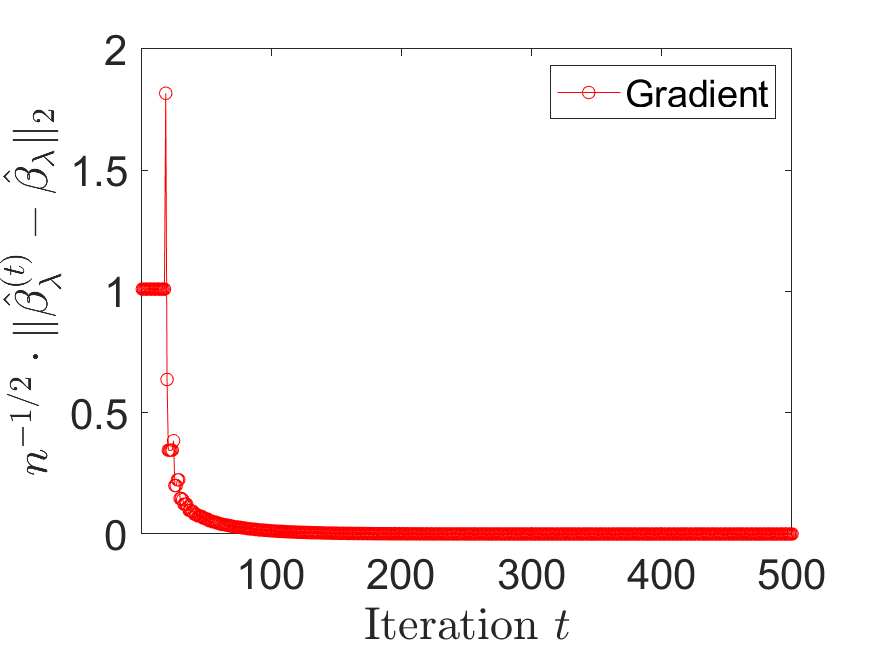
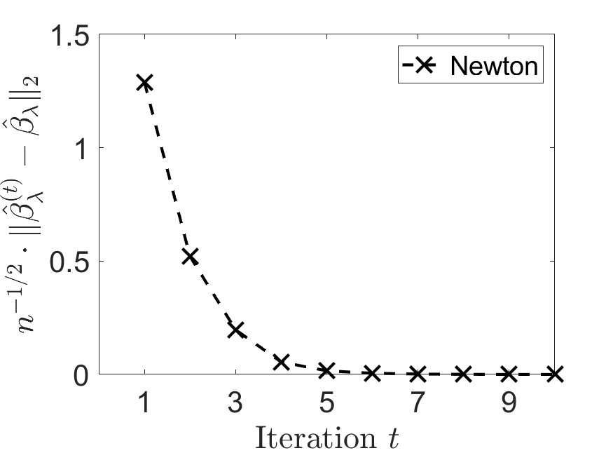
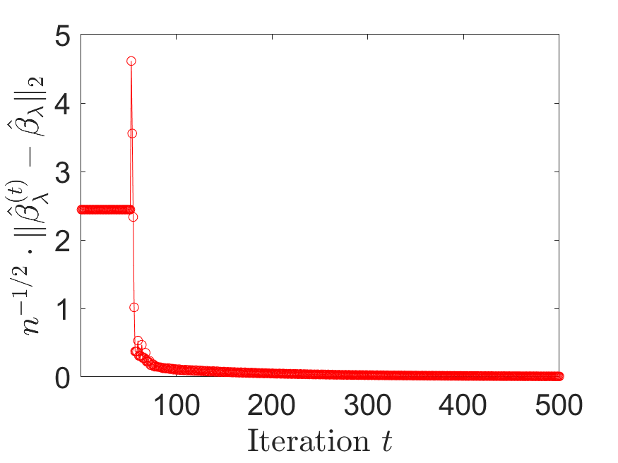
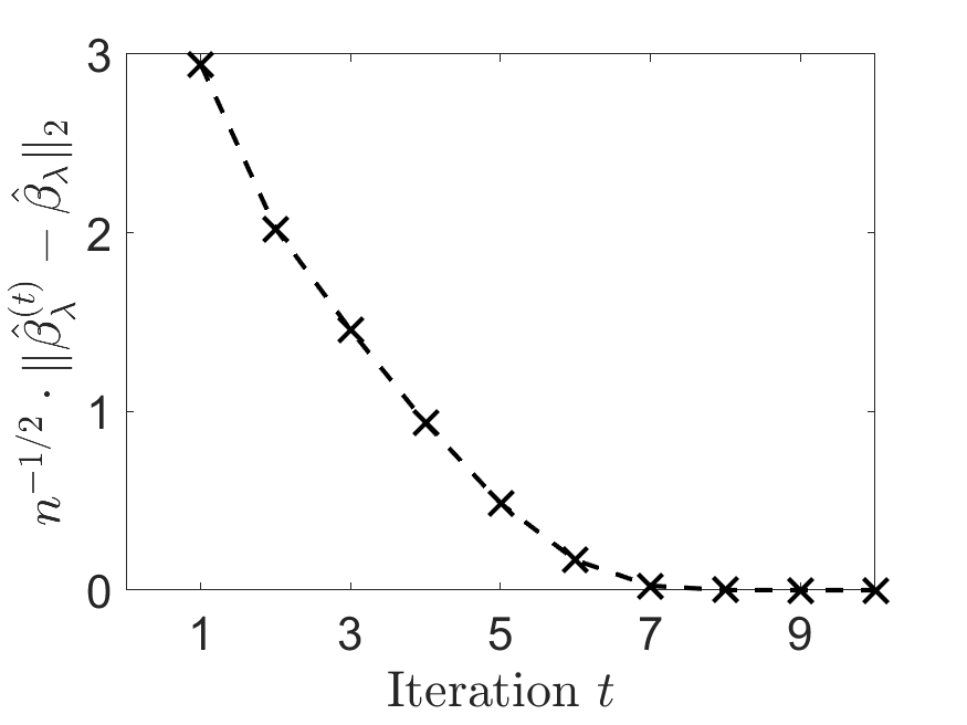
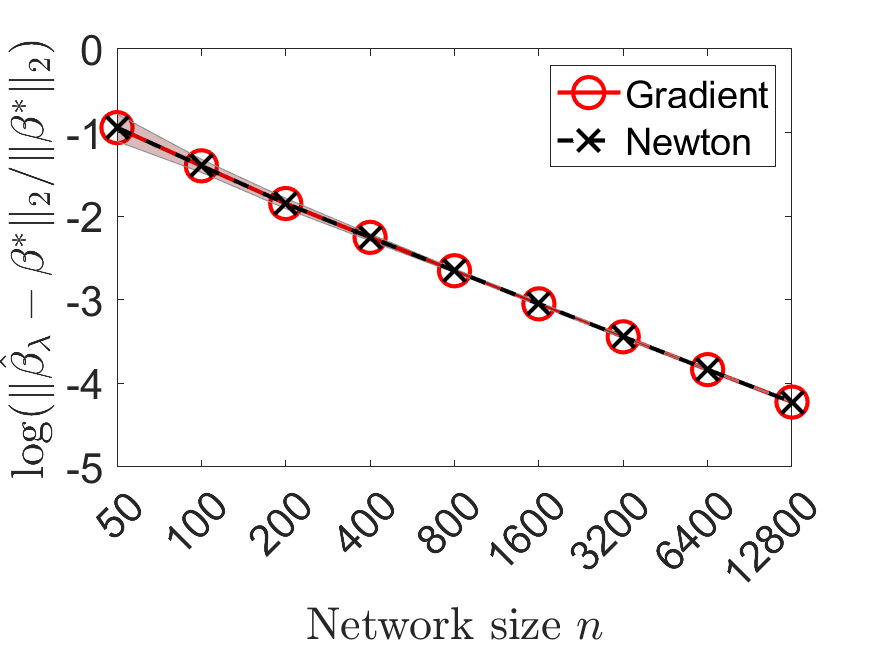
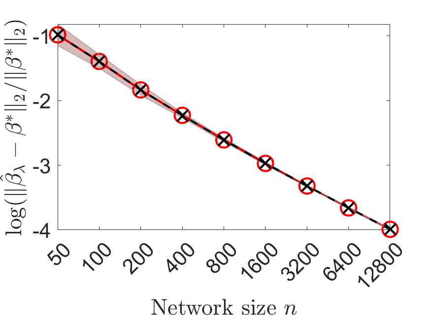
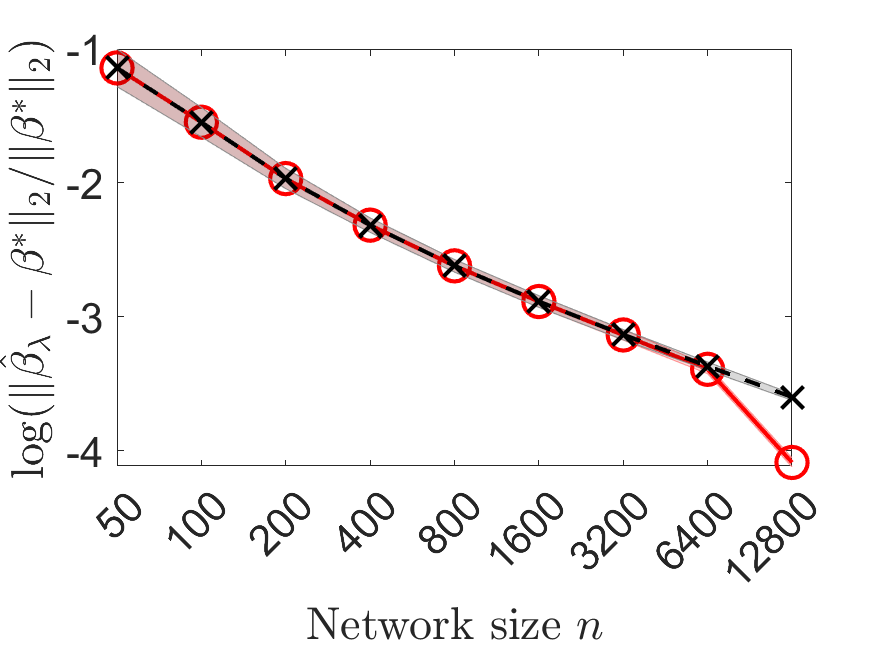
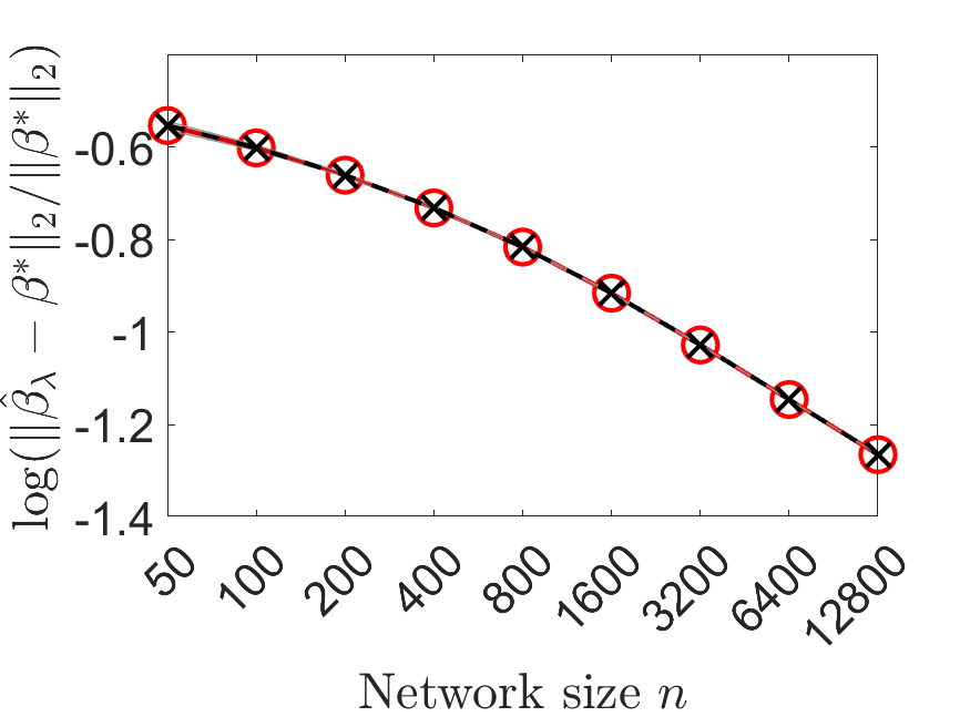
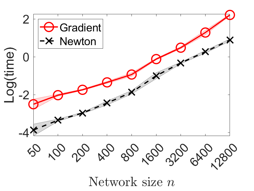
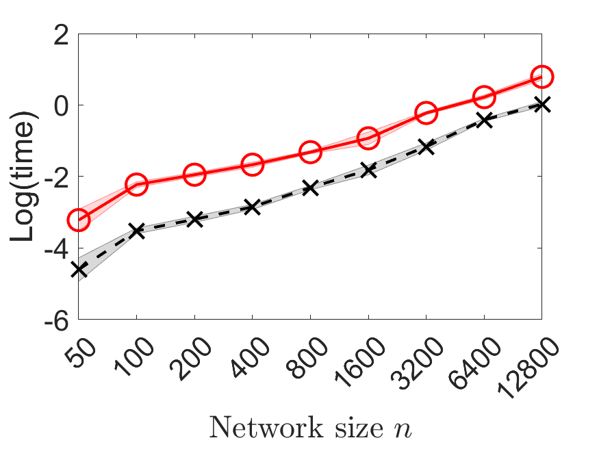
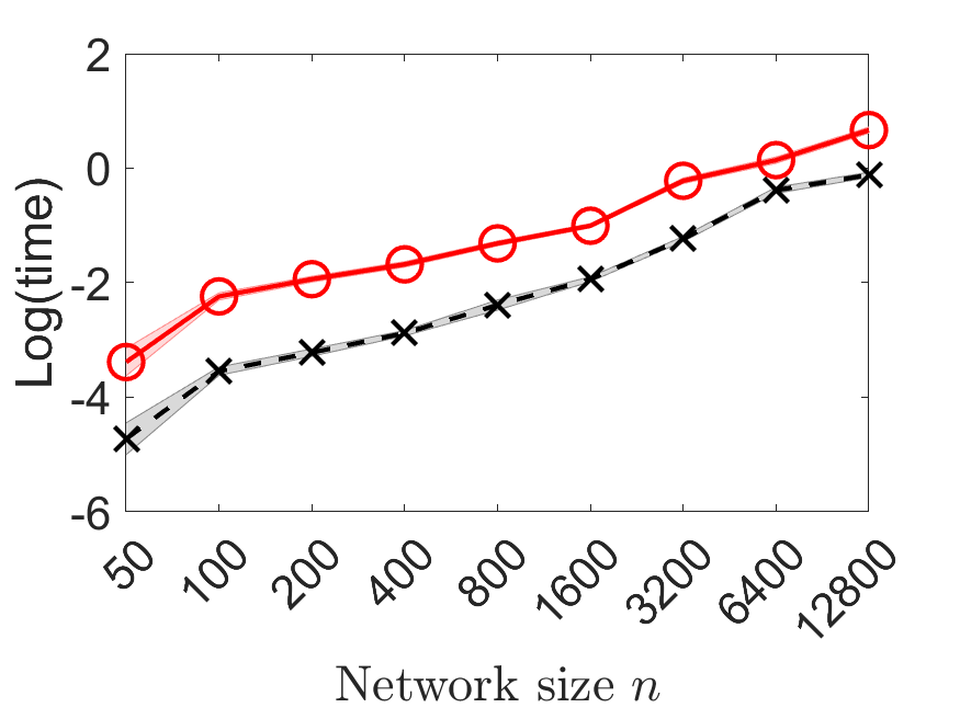
Figure 1: Row 1: convergence speed, setting (i), plots 1 & 2: $n=50$, 3 & 4: $n=12800$; plots 1 & 3: gradient, 2 & 4: Newton; Row 2: log average $\ell_{2}$ errors, from left: settings (i)–(iv); Row 3: computation time, from left: settings (i)–(iv).

Next, we show simulation plots that validate our Theorem 5. We first check the intercept term. For this purpose, we plot the one-dimensional marginal empirical distributions of $\widehat{\beta}_{\lambda;1}$ under our simulation settings (i) and (vi) in Table 3, respectively. We range $n\in\{100,400,\cdots,6400\}$. The results are reported in Figure 2. Row 1 of Figure 2 corresponds to dense networks, where we set a small $\lambda=0.1$; and in row 2, we set a large $\lambda=2n$. The results verify that our prediction of the intercept in Theorem 5 is accurate.

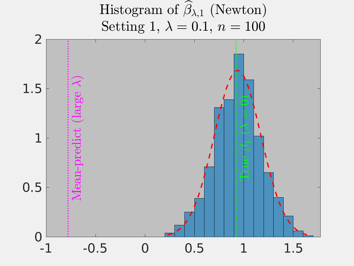
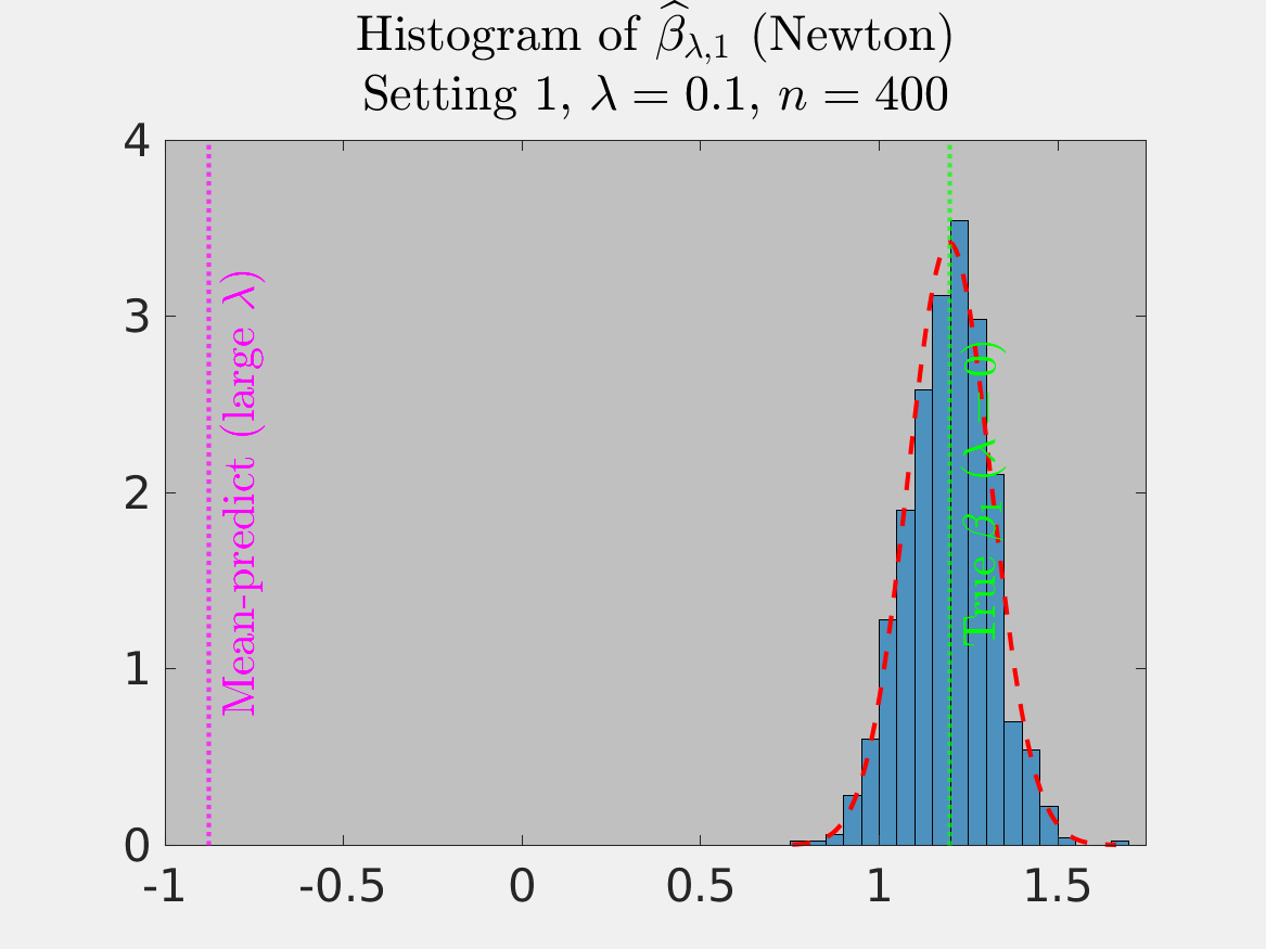
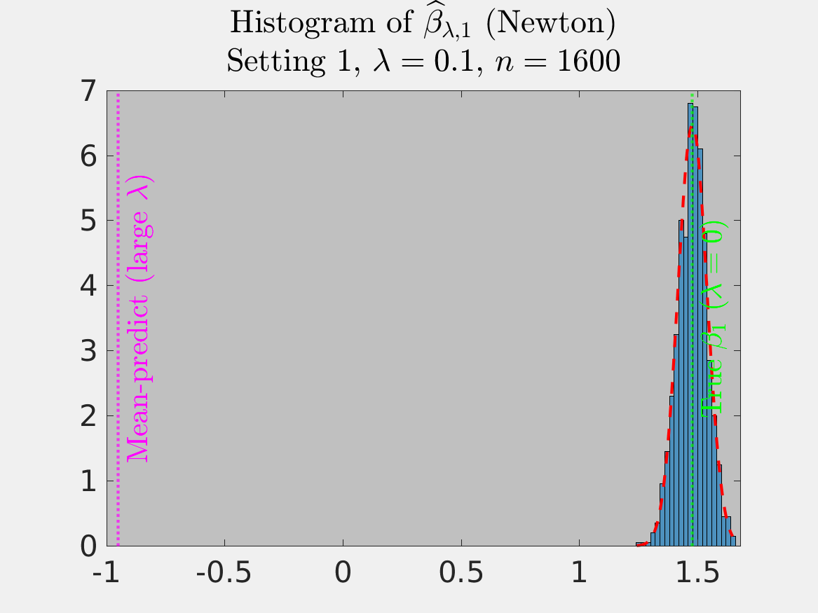
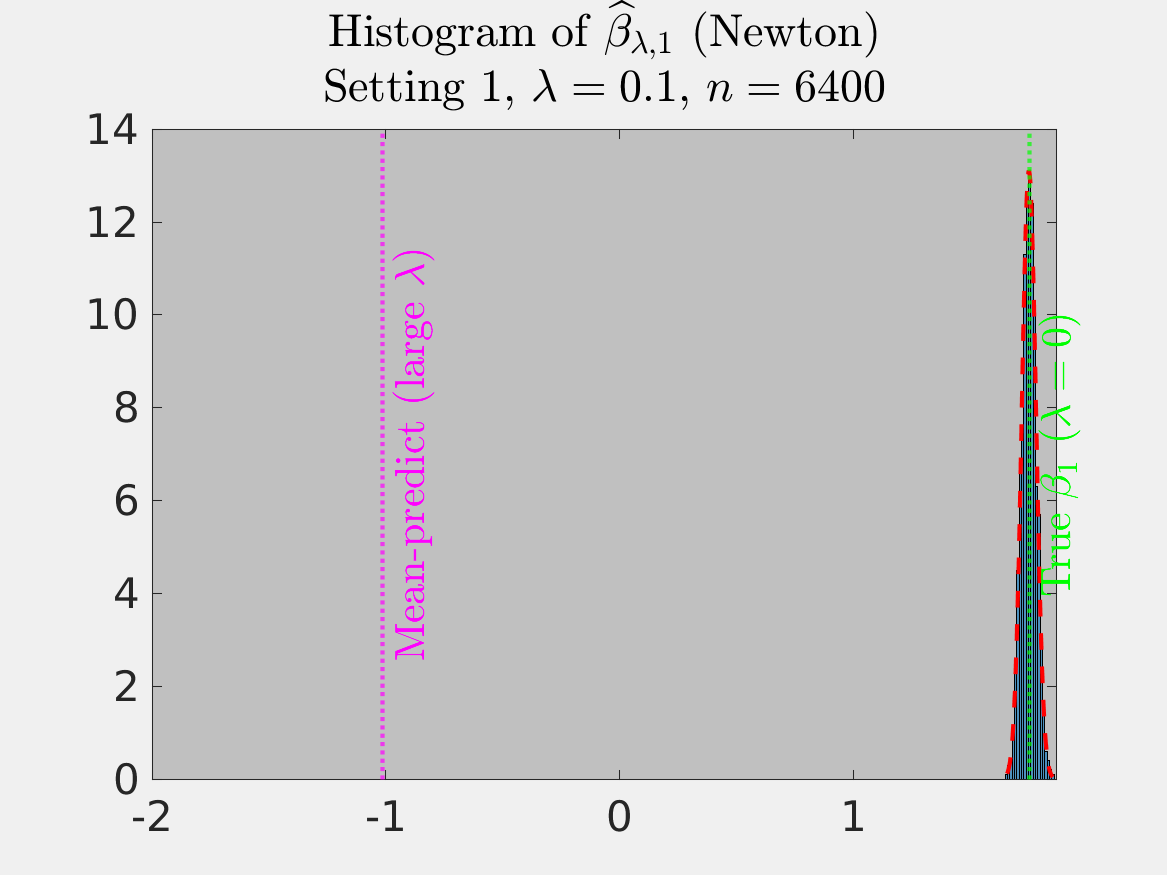
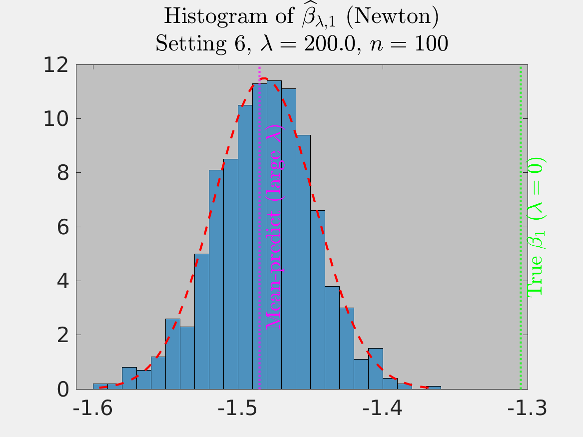
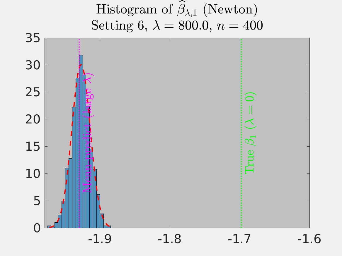
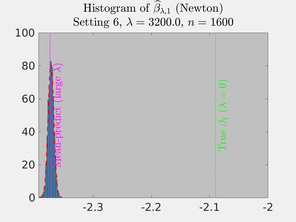
Figure 2: Asymptotic distributions of $\widehat{\beta}_{\lambda;1}$ under various $n$ for tuning parameter $\lambda$. Row 1: setting 1 (moderately dense network, small $\lambda$); row 2: setting 6 (sparse network, large $\lambda$). Green line: mean prediction for small $\lambda$ case; magenta line: mean prediction for large $\lambda$ case.

Next, we validate our Theorem 5’s prediction of the variance term. Then, we illustrate the dependency structure between $\widehat{\beta}_{\lambda;n-1}$ and $\widehat{\beta}_{\lambda;n}$ under our settings (iii) – (v). The simulation results presented in Figure 3 provide clear empirical evidences that well-match our novel normality result Theorem 5. Traveling from the left to the right in Row 1 of Figure 3, as $\lambda$ increases with other settings fixed, we see an increasing correlation between $\widehat{\beta}_{\lambda;n-1}$ and $\widehat{\beta}_{\lambda;n}$, exactly as Part (ii) of our Theorem 5 predicts. Traveling from the right-most plot in Row 1 and then continue from the left in Row 2, we are increasing $n$ with a fixed $\lambda$. This is roughly equivalent to decreasing $\lambda$ and traveling from large $\lambda$ back to small $\lambda$. In this comparison sequence, we clearly see an increasing independence, which again confirms the prediction of our Theorem 5.

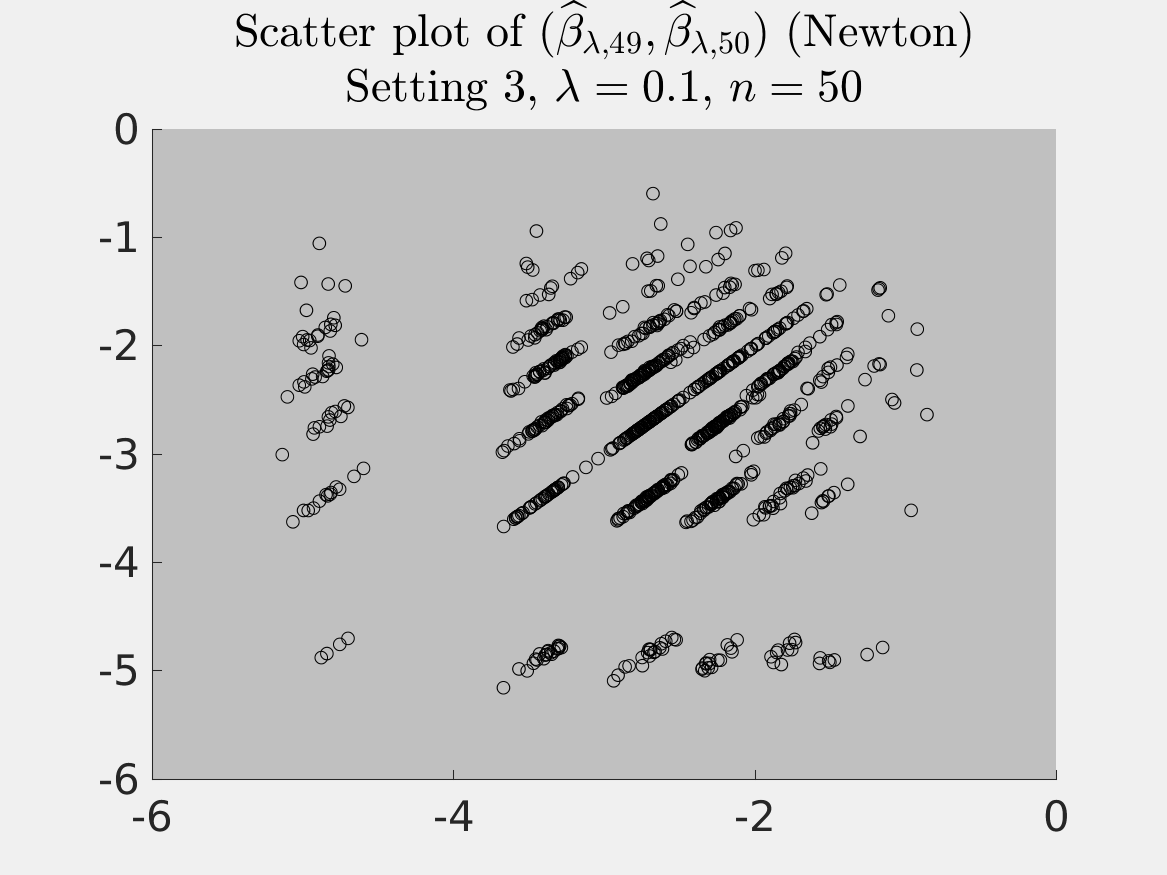
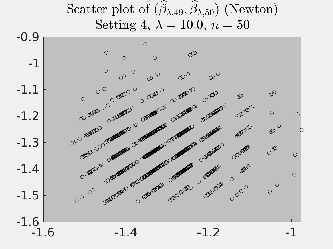
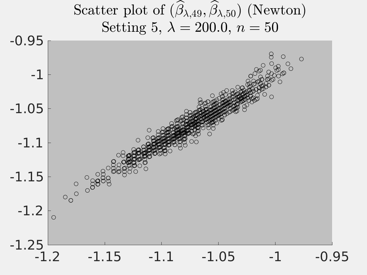
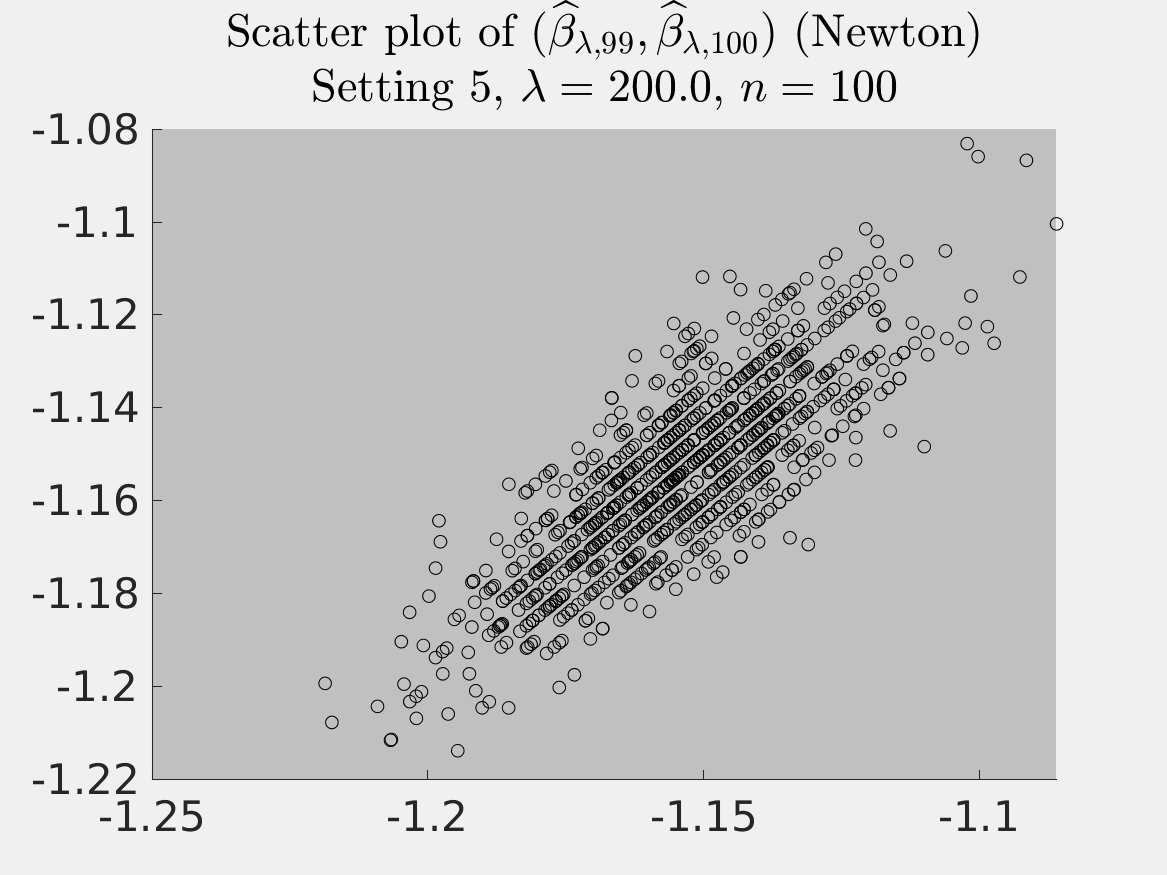
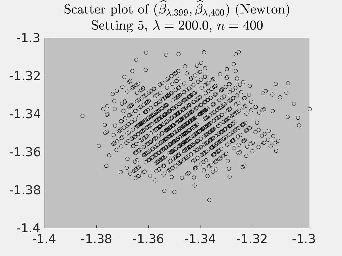
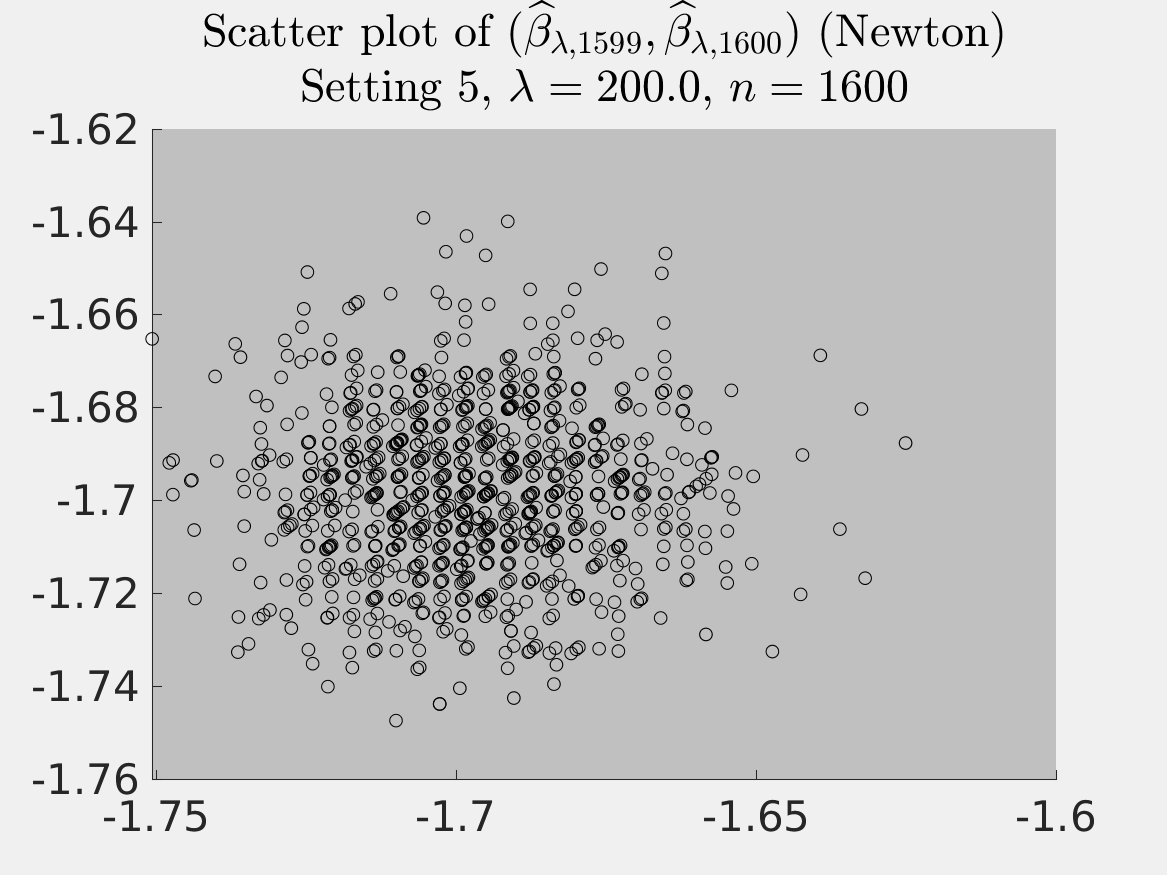
Figure 3: Joint distribution of $(\widehat{\beta}_{\lambda;n-1},\widehat{\beta}_{\lambda;n})$. Row 1: fix $n=50$ and increase $\lambda\in\{0.1,10,200\}$; row 2: fix $\lambda=200$ and increase $n\in\{100,400,1600\}$; other simulation set-ups are identical across all 6 plots.

5.2 Simulation 2: performance comparison to $\ell_{0}$ and $\ell_{1}$ regularization methods

In this simulation, we compare our proposed $\ell_{2}$-regularized MLE to the $\ell_{0}$ (Chen et al., 2021) and $\ell_{1}$ Stein and Leng (2020) regularization methods. We consider the following settings with different network sparsity levels:

$$\beta^{*}_{i}= ~{}(-0.2\log n)/2+\mathbbm{1}_{[i\in\{1,\cdots,[n/10]\}]}(0.4\log n)+\mathbbm{1}_{[i\in\{[n/10]+1,\cdots,[n/5]\}]}(-0.4\log n),$$ (35)

$$\beta^{*}_{i}= ~{}(-0.6\log n)/2+\mathbbm{1}_{[i\in\{1,\cdots,[n/20]\}]}(0.2\log n)+\mathbbm{1}_{[i\in\{[n/20]+1,\cdots,[n/10]\}]}(-0.2\log n).$$ (36)

We varied network size $n\in\{100,200,\cdots,3200\}$ and evaluate the performance of the $\widehat{\beta}$’s produced by all three methods in the following five aspects: (1) $n^{-1}\|\widehat{\beta}-\beta^{*}\|_{1}$; (2) $n^{-1/2}\|\widehat{\beta}-\beta^{*}\|_{2}$; (3) $\|\widehat{\beta}-\beta^{*}\|_{\infty}$; (4) the relative error in estimating the ”active set” ${\cal S}$ (${\cal S}=[1:[n/5]]$ in the dense network setting, and ${\cal S}=[1:[n/10]]$ in the sparse network setting), denoted by the Hamming distance between $\widehat{\cal S}$ and ${\cal S}$, divided by $n$; and (5) computation time; where in (4), we employ the post-estimation thresholding method described in our Corollary 1 to obtain $\widehat{\cal S}$ for our method. In each setting, we repeated the experiment 1000 times for our method and 100 times for the other two methods due to their much higher computation costs.

Figure 4 shows the result. Row 1 corresponds to the denser network setting (35), where we set $\lambda=0$. Our method shows steadily achieves the best or a competitive accuracy across all settings. Specifically, unlike Chen et al. (2021) and Stein and Leng (2020), our thresholding method for estimating ${\cal S}$ does not require that $\beta_{i}^{*}-\beta_{j}^{*}>0$ for all $i\in{\cal S}$, $j\notin{\cal S}$. This explains the advantage of our method in estimating the sparsity structure of $\beta^{*}$ compared to these methods. Notice that the parameter estimation accuracy of both Chen et al. (2021) and Stein and Leng (2020) depends on their accurate specification of the sparsity structure in $\beta^{*}$, whereas our method does not. The fifth plot shows a clear speed advantage of our method. Chen et al. (2021) and Stein and Leng (2020) could not handle networks over $n=10^{3}$ effectively and require an infeasible amount of memory when $n\approx 10^{4}$ and could not finish even one run. In our repeated experiments, they start to time out earlier as $n\asymp 10^{3}$.

The results shown in row 2 can be interpreted similarly to row 1. In row 2, we tested different choices of $\lambda$ for our method. Despite the higher network sparsity level compared to row 1, choosing a small positive $\lambda$ still yields the best performance across all measurements in row 2. This echoes the interpretation of our Theorems 1 and 2. We generally do not recommend choosing a large $\lambda$, unless the network is extremely sparse and we believe the true $\beta^{*}$ is approximately parallel to $\mathbbm{1}$. Indeed, our method with a very large $\lambda=n\log n$ effectively fits a nearly Erdos-Renyi model to the data. The results here also matches the prediction of our main theorems. For example, all $\ell_{p}$ errors diverge, and our theorem predicts the $\ell_{p}$, $p=2,\infty$ upper bounds to be $n^{-1/p}\cdot\|{\cal P}_{\perp}\beta^{*}\|_{p}$, $p=2,\infty$, both of which also diverge at the rate of $\log n$ in this simulation.

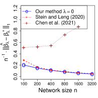
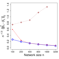
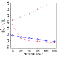
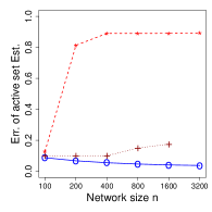
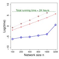
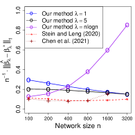
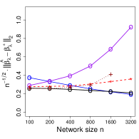
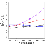
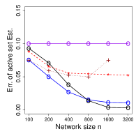
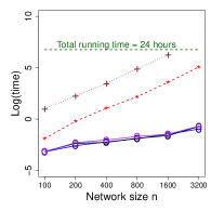
Figure 4: Performance comparison with benchmark methods. Row 1: setting (35); row 2: setting (36).

5.3 Simulation 3: performance of our AIC-type criterion for tuning $\lambda$

Here, we assess the correctness of our AIC-type criterion, proposed in Section 4, in automatically tuning $\widehat{\beta}_{\lambda}$. We generate data from dense and sparse networks with the following specifications:

$$\beta_{1}^{*}=\cdots=\beta_{[n/10]}^{*}=-1/5\log n, \quad\beta_{[n/10]+1}^{*}=\cdots=\beta_{n}^{*}=1/2\log n,$$

$$\beta_{1}^{*}=\cdots=\beta_{[n/3]}^{*}=-1/3\log n, \quad\beta_{[n/3]+1}^{*}=\cdots=\beta_{n}^{*}=(-1/3+0.05)\log n.$$

Figure 5 shows that the tracks of the rescaled versions of our AIC-type criterion’s values is consistent with the relative $\ell_{2}$ errors of $\widehat{\beta}_{\lambda}$ under different $\lambda$ choices. For the first setting where the network is dense, it suggests $\lambda=0$; whereas in the latter setting with a sparse network, it selects a large $\lambda$.

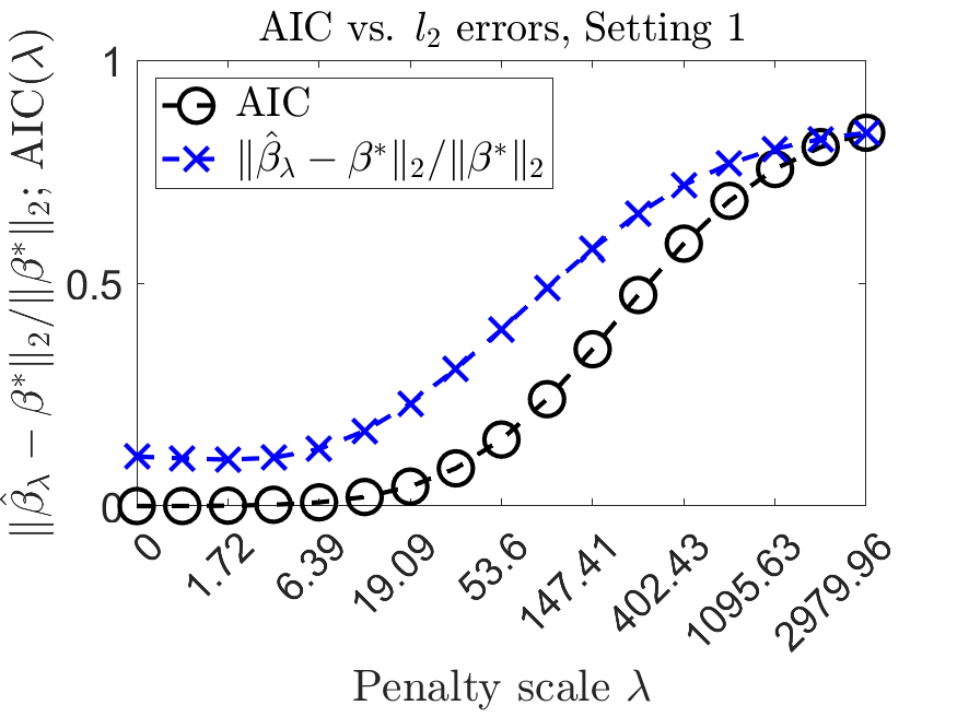
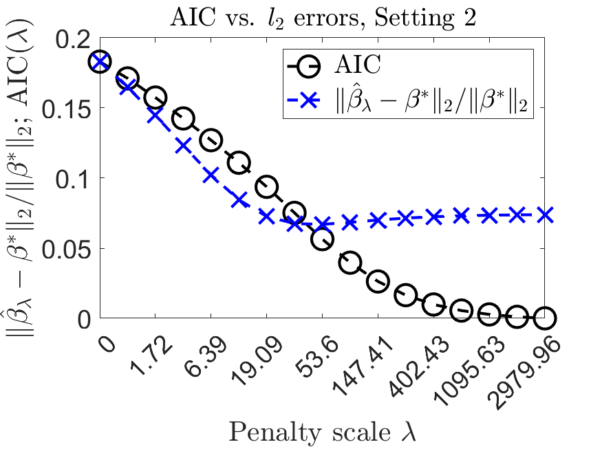
Figure 5: Tuning $\lambda$ under large (left) and small (right) $\|{\cal P}_{\perp}\beta^{*}\|_{2}$ values. Blue curve: true estimation error $\|\widehat{\beta}_{\lambda}-\beta^{*}\|_{2}/\|\beta^{*}\|_{2}$; black dashed curve: AIC-type criterion AIC$(\lambda)$. The black curve has been rescaled, such that it has the same highest point as the blue curve. The original heights of black and blue curves are very different.

6 Data examples

6.1 Data example 1: impact of COVID-19 on Swiss student mental health

The data set Elmer et al. (2020) contains social and psychological measurements on a local group of Swiss students to assess the impact of COVID-19 pandemic lockdown on their mental health. The original data set contains two cohorts of students dated 2019-04 (cohort 1), 2019-09 (cohort 2) and 2020-04 (cohort 2). For better comparability, we select the 2019-09 and 2020-04 subgroups since they share many individuals in common; while the 2019-04 data were surveyed on a distinct group of students longer before the pandemic. The variables fall into two main categories: 1. mental health, including depression, anxiety, stress and loneliness; 2. sociality, encoded by students’ self-reported number of other students, with whom they have the following types of relations: friendship, pleasant interactions, emotional support, informational support and co-study.

First, as aforementioned, the released data only disclose node degrees, rather than adjacency matrices. This renders GLM-based methods such as Yan et al. (2019); Stein and Leng (2020) inapplicable. Second, not all students show up in both subgroups. The two subgroups contain 207 (2019-09) and 271 (2020-04) students, respectively, sharing 202 students in common. To make the most use of available data, we perform two marginal analysis on the two subgroups, respectively, then perform a differential analysis to compare the estimated parameters on the common students.

Variable	friend	p.interaction	e.support	inf.support	co-study
Mean degree (2019-09)	3.928	6.454	1.444	2.019	2.048
Std. dev. (2019-09)	(2.554)	(4.225)	(1.503)	(1.692)	(2.004)
Mean degree (2020-04)	4.007	5.657	1.590	2.173	1.694
Std. dev. (2020-04)	(2.878)	(3.810)	(1.749)	(1.835)	(2.071)

Table 4: Network degree statistics, each column represents a different sociality network.

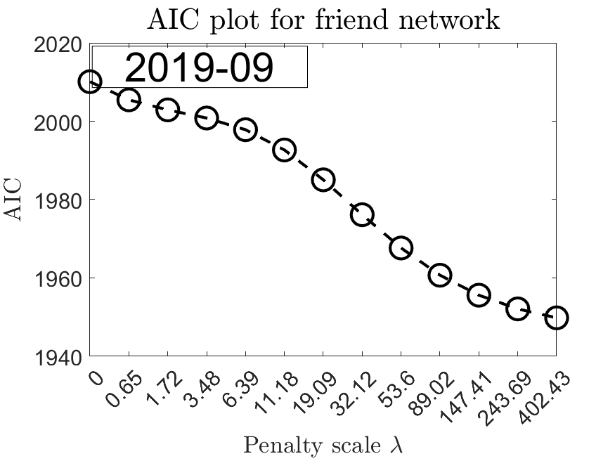
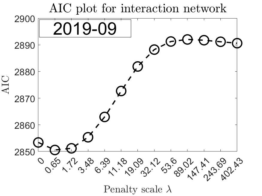
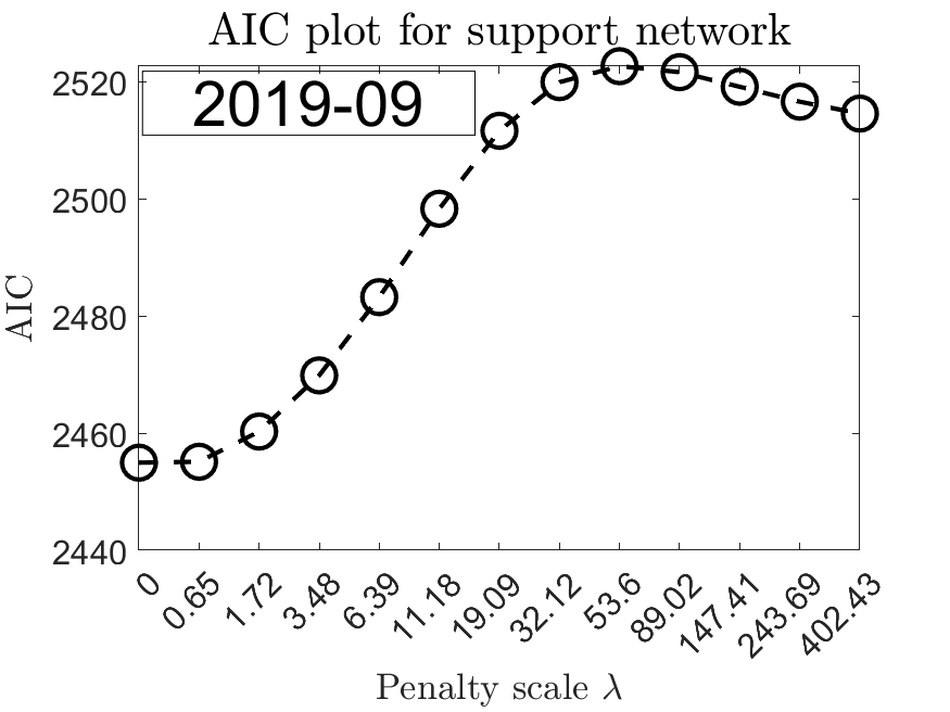
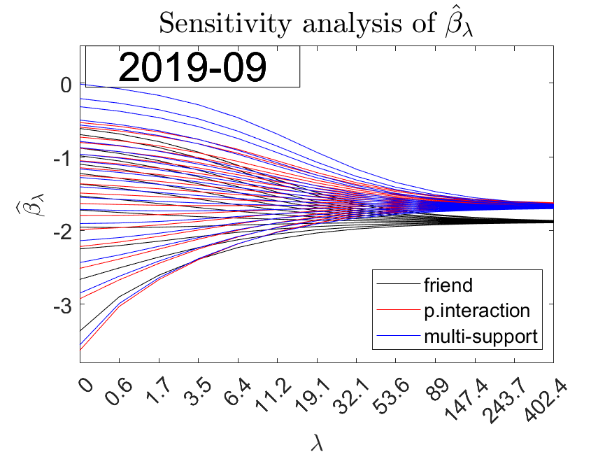
Figure 6: Left three panels: AIC plots for tuning $\lambda$; right panel: tracks of $\widehat{\beta}_{\lambda}$ over different $\lambda$ choices. The left-most panel suggests that the friendship networks are too sparse for informative $\beta$-model fits.

The third consideration is that both networks, despite their small sizes, are very sparse, as shown in Table 4, especially the emotional support, informational support and co-study networks. To alleviate this sparsity, we combined the three networks by summing up the degrees of each node in each subgroup as support network, resulting average degrees of $5.51(4.33)$ (2019-09) and $5.46(4.63)$ (2020-04), respectively. Degree distributions suggest that $\beta_{i}$’s might not be $\ell_{0}$-sparsity, and our proposed $\ell_{2}$-regularized MLE with a small $\lambda$ seems appropriate. We removed isolated nodes in each network and fit $\beta$-models to the social networks, with candidate choices of $\lambda\in\{0,e^{0.5}-1,\cdots,e^{6}-1\}$. The first three columns in Figure 6 show the AIC curves for each type of social network in the two subgroups respectively. The friendship network turns out to be too sparse that our AIC criterion suggests choosing a large $\lambda$, and this will lead to an estimation with similar $\widehat{\beta}_{\lambda;i}$’s for all nodes. It is also conceptually difficult to combine with other networks, so we do not consider the friend network in our following analysis. As for the other two networks, the AIC plots suggest choosing $\lambda=0.65$ for the interaction network and $\lambda=0$ for the support network, respectively.

Recall our goal is to study the relationship between mental health and sociality. We treat the $\widehat{\beta}_{\lambda}$’s estimated from different networks as covariates and perform a sparse canonical correlation analysis (CCA) (Witten et al., 2009) between mental health variables and our estimated sociality $\beta$ parameters on three data sets: 2019-04, and 2020-09 and the difference in their corresponding covariate values over their common nodes. For this part, we employ the CCA function in the R package PMA (Witten et al., 2009) and let it automatically tune the penalty term for its $\ell_{1}$-penalized sparse CCA procedure. To assess the significance of each individual CCA coefficient, we employ a bootstrap procedure that repeatedly randomly shuffles the rows of mental health variables, while keeping the row order of sociality variables, and compute its empirical p-values.

The results are reported in Table 5, where we print the first two canonical components. They mainly capture the connections between each of the two social networks (support and pleasant interaction) and mental health covariates, respectively. Before the lockdown, loneliness was the most prominent factor. Its almost opposite correlation directions with the two types of social networks might possibly be explained by that students tend to prefer pleasant interactions with friends rather than information support or co-study interactions, when they feel lonely. After the lockdown, stress became the most important factor that positively correlates with both pleasant interaction and support networks; while loneliness faded out. This is understandable, since many students might have to worry more about practical problems including study and job hunting, therefore might pay less attention to loneliness. The third main column in Table 5 shows the canonical correlations between the difference in mental health and the difference in sociality variables. Combined with Figure 2 in Elmer et al. (2020), we understand the result in this part as that increased loneliness and anxiety levels led to higher demands for pleasant interaction and support, respectively.

Marginal Common nodes 2019-09 2020-04 Difference Variable CC1 p-val. CC2 p-val. CC1 p-val. CC2 p-val. CC1 p-val. CC2 p-val. depression $-$0.005 (0.424) 0.183 (0.316) 0.000 (0.420) 0.049 (0.371) 0.399 (0.278) 0.000 (0.459) anxiety 0.453 (0.288) 0.139 (0.377) 0.529 (0.289) 0.181 (0.361) 0.000 (0.460) 0.941 (0.179) stress $-$0.051 (0.404) $-$0.065 (0.396) 0.848 (0.217) 0.960 (0.161) $-$0.089 (0.425) 0.295 (0.353) loneliness $-$0.890 (0.244) 0.971 (0.149) $-$0.023 (0.448) 0.210 (0.385) 0.913 (0.193) 0.164 (0.409) p.interaction 0.000 (0.506) 1.000 (0.000) 0.000 (0.508) 1.000 (0.000) 1.000 (0.000) 0.000 (0.505) support 1.000 (0.000) 0.000 (0.494) 1.000 (0.000) 0.000 (0.492) 0.000 (0.495) 1.000 (0.000)

Table 5: Estimated sparse CCA coefficients with empirical p-values.

6.2 Data example 2: analysis of two very large COVID-19 knowledge graphs

In this subsection, we apply our fast algorithm in Section 2.2 to two very large COVID-19 knowledge graphs. These applications demonstrate our method’s significant superiority in speed and memory.

The first data set Steenwinckel et al. (2020) was transcribed from the well-known Kaggle CORD-19 data challenge in 2020. We downloaded the data from https://www.kaggle.com/group16/covid19-literature-knowledge-graph, which contains $n=1304155\approx$ 1.3 million nodes. The second data set Wise et al. (2020) is part of the open-access Amazon data lake that is still updating real-time at the frequency of several times per hour. We analyze the version downloaded at 20:06pm UTC on 15th September, 2021. After cleaning up, the citation network contains $n=57312$ papers (nodes). The reason we choose to study these two particular COVID-19 knowledge graph databases is that they are well-documented and maintained. The sizes of these data are prohibitive for the conventional GLM-based algorithms for fitting $\beta$-models (Yan et al., 2015; Chen et al., 2021; Stein and Leng, 2020, 2021), which typically need hours to compute networks of a few thousand nodes. In sharp contrast, our code costs less than 10 minutes on a personal computer to estimate for Steenwinckel et al. (2020).

Both data sets are structured following the typical knowledge graph fashion. The raw data are formatted in such 3-tuples: (entity 1, relation, entity 2), for example, (paper 1, cites, paper 2), (paper 1, authored by, author 3), (author 4, membership, institution 7) and so on. In this study, we focus on the paper citation network (paper 1, cites, paper 2) and ignore edge directions like that has been done in Li and Yang (2021) and Liu et al. (2019). Indeed, there are many interesting scientific problems that can potentially be addressed with these data sets. Due to page and scope limits, in this paper, we focus on findings based on $\beta$-model fits.

6.2.1 Data set 2a: the ISWC 2020 transcription of Kaggle CORD-19 data challenge

We first analyze the transcribed Kaggle data set (Steenwinckel et al., 2020). Compared to the Amazon data set Wise et al. (2020), Steenwinckel et al. (2020) has a larger citation network but fewer nodal covariates and no map between papers and topics (keywords). Therefore, its analysis is comparatively simpler. However, in this ISWC transcription of Kaggle data, most of the 1.3 million nodes in the complete network here are not on COVID-19 but general medical literature. We would use the complete network to estimate $\widehat{\beta}_{\lambda}$; afterwards, we use metadata.csv in Kaggle CORD-19 open challenge downloaded from https://www.kaggle.com/datasets/allen-institute-for-ai/CORD-19-research-challenge to filter and only keep COVID-19 papers, similar to the treatment in Rausch (2020).

Here, we focus on the nodal covariate country and compare the empirical distributions of $\widehat{\beta}_{\lambda}$ entries corresponding to different countries. We selected 6 representative countries/regions in the study of pandemic: UK, China, USA, EU (we counted France, Germany, Italy, Spain, Switzerland and Netherlands, which constitute the overwhelming majority of papers from EU), Japan plus South Korea, and India. All other papers are collected by the “Other” category. To choose a proper tuning parameter, we vary $\lambda\in\{0,1,2.5,\cdots,1280\}$ and plot the track of AIC$(\lambda)$ and $\widehat{\beta}_{\lambda}$ in Figure 7. Our AIC-type criterion suggests choosing $\lambda=0$. Then we run our accelerated Newton’s method on the complete network, and filter $\widehat{\beta}_{\lambda}$ entries using CORD-19 metadata as aforementioned.

Figure 7: Tracks of AIC$(\lambda)$ and $\widehat{\beta}_{\lambda}$, Left two panels: Steenwinckel et al. (2020); right two panels: Wise et al. (2020)

Table 6: Estimated $\widehat{\beta}_{\lambda}$ by region

Region	Other	China	US	UK	EU	JpKr	India
Entry count	53929	6096	15169	4747	11180	2394	1450
mean($\widehat{\beta}_{\lambda}$)	$-$5.426	$-$4.426	$-$4.477	$-$4.590	$-$4.553	$-$4.507	$-$4.737
std($\widehat{\beta}_{\lambda}$)	(1.417)	(1.018)	(1.104)	(1.099)	(1.084)	(1.048)	(1.172)

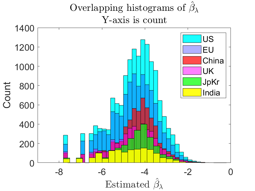
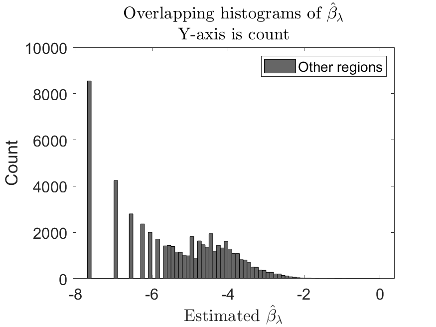
Figure 8: Overlapping histograms of estimated $\widehat{\beta}_{\lambda}$ by region

Table 6 reports the numerical summary of estimation results and Figure 8 shows the region-wise histograms. Second, despite different total paper counts, the $\widehat{\beta}_{\lambda}$ distributions across the 6 regions we studied show similar marginal distributions. Inspecting the raw data, we understand that this can be partially attributed to the active international collaboration and mutual citation. Overall, we see from Figure 6 the clear evidence of solidarity and impartiality among scientists and researchers studying COVID-19.

6.2.2 Data set 2b: the Amazon public COVID-19 data lake, knowledge graph section

The Amazon public COVID-19 data lake Wise et al. (2020) documents less papers ($n=57312$) than Steenwinckel et al. (2020), but provides richer details on each entry, including a list of “topics”, which can be understood as key words that are not specified by the authors but automatically learned by a latent Dirichlet allocation (Blei et al., 2003) text analysis (see the “Graph Structure” section of Kulkarni et al. (2020)). The outcome can be represented as a list for paper $i$: $\{\textrm{topic}_{j}^{(i)}:s_{j}^{(i)}\}_{j=1,\ldots,k_{i}}$, where $s_{j}^{(i)}\in[0,1]$ is a score indicating the relevance of the topic. Here, we are interested in finding the “core” and “peripheral” topics in current literature. Our approach is to propose a “Weighted Accumulative Beta Score (WABS)”. For each concept $j$, let ${\cal A}_{j}\subseteq\{1,\ldots,n\}$ be the index set of all papers that specify $j$ in its relevant topic list, and $s_{j}^{(i)}$ be the corresponding relevance score reported in the data set. We define

$$\textrm{WABS}_{j}=\sum_{i\in{\cal A}_{j}}{\color[rgb]{0,0,0}e^{\widehat{\beta}_{\lambda;i}}}\times s_{j}^{(i)}.$$ (37)

Now we briefly explain the intuition behind the definition of (37). On one hand, we design it as a sum, rather than an average, because the total count carries useful information and should be reflected in the measure. On the other hand, however, we also want to prevent “quantity over quality” by re-weighting each relevance score $s_{j}^{(i)}$ by the paper’s transformed global popularity $e^{\widehat{\beta}_{\lambda;i}}$. In plain words, for a topic to sit at the center of the knowledge base, not only it should be a closely relevant topic of many papers, but further, it needs to be associated with many influential papers. One influential paper’s contribution to the right hand side of (37) could easily outweigh connections to many peripheral works. Similar to the aforementioned point in our analysis of data example 1 (Elmer et al., 2020), our proposed WABS measure inherits the scale-free advantage from $\widehat{\beta}_{\lambda}$, thus is comparable across networks of potentially very different sizes.

Table 7: Summary statistics for top- and bottom-50 concepts, ranked by Weighted Accumulative Beta Score (WABS)

Top 50 Bottom 50 Concept Category Paper # Avg($d_{i}$) WABS Concept Category Paper # Avg($d_{i}$) WABS infection dx name 18558 10.66 319.85 méthicilline dx name 1 3.00 0.01 respiratory syndrome dx name 6951 13.49 158.09 icer dx name 2 2.00 0.01 death dx name 7689 10.92 126.06 colostrum dx name 3 1.67 0.01 lung system organ site 6051 12.50 121.56 economic injury system organ site 2 2.50 0.01 respiratory tract system organ site 5094 14.53 117.10 cellmediated immunity system organ site 2 2.50 0.01 pneumonia dx name 4696 14.40 115.15 mesenteric lymphatic dx name 2 2.00 0.01 fever dx name 5531 12.11 111.01 perianal infection dx name 2 1.50 0.01 viral infection dx name 6669 11.02 109.37 psychiatric treatment dx name 3 1.67 0.01 culture test name 5739 11.02 92.63 potassium ion test name 1 5.00 0.01 cough dx name 3794 13.37 85.58 lysine decarboxylase dx name 2 2.00 0.01 die dx name 4194 12.46 84.92 fibrosis progression dx name 3 1.67 0.01 vaccine treatment name 5328 11.22 83.53 gldh treatment name 2 1.50 0.01 infect dx name 5852 11.90 82.11 neurobehavioral disorder dx name 1 3.00 0.01 liver system organ site 3910 11.09 69.14 nr2b system organ site 2 2.00 0.01 diarrhea dx name 3244 12.59 67.96 TRA dx name 2 2.50 0.01 hand system organ site 5347 9.37 67.51 hcv replicon assay system organ site 2 2.50 0.01 kidney system organ site 3213 13.31 66.10 Methylprednisolon system organ site 3 1.00 0.01 HIV dx name 4678 9.16 65.55 platelet index dx name 2 1.50 0.01 respiratory infection dx name 3081 13.46 65.07 immune tissue dx name 2 2.00 0.01 respiratory disease dx name 2686 15.10 61.62 herpetic uveitis dx name 2 1.50 0.01 respiratory syncytial virus dx name 2900 12.91 54.82 cadpr dx name 2 2.50 0.01 chest system organ site 2159 14.99 53.93 rna expression profiling system organ site 3 1.67 0.01 rt-pcr test name 2613 15.71 53.55 demostraron test name 2 2.00 0.01 infectious disease dx name 4766 8.55 51.79 tnfsf4 dx name 1 3.00 0.01 throat system organ site 2201 14.78 50.78 boutonneuse fever system organ site 2 2.50 0.01 heart system organ site 2955 10.64 50.61 mucopolysaccharide system organ site 3 1.33 0.01 pcr test name 3381 11.65 50.27 urethral mucosa test name 2 1.50 0.01 lesion dx name 2586 11.38 47.47 covariance analysis dx name 3 1.33 0.01 titer test name 2681 12.25 47.05 transfusion-associated circulatory overload test name 2 2.50 0.01 influenza virus dx name 3401 10.20 45.76 Chondrex dx name 3 1.33 0.01 inflammation dx name 3500 8.51 45.29 tea dx name 3 1.67 0.01 phylogenetic analysis test name 1825 16.37 43.70 oxidovanadium test name 2 1.50 0.01 vomiting dx name 1869 13.33 42.37 anti-tnf$\alpha$ drug dx name 1 4.00 0.01 respiratory tract infection dx name 2076 13.84 41.19 control assay dx name 2 2.50 0.01 penicillin generic name 2534 9.63 40.83 avanzadas generic name 3 1.33 0.01 adenovirus dx name 2275 12.65 40.71 dystrophic neurite dx name 3 1.67 0.01 respiratory distress syndrome dx name 1248 19.52 39.50 gastric erosion dx name 2 1.50 0.01 ribavirin generic name 1254 18.20 39.21 foetal loss generic name 3 1.33 0.01 antibiotic generic name 3094 9.42 38.68 alloreactive t cell generic name 2 2.50 0.01 rsv dx name 2345 11.79 38.49 cefuroxima-axetilo dx name 2 2.00 0.01 serum sample test name 1822 13.51 37.97 cerebrovascular complication test name 1 3.00 0.01 respiratory illness dx name 1668 15.17 37.39 inadequate tissue oxygenation dx name 2 2.50 0.01 respiratory virus dx name 2101 13.47 36.86 il-1$\beta$ concentration dx name 1 3.00 0.01 streptomycin generic name 2139 9.93 35.78 hypertransfusion generic name 1 3.00 0.01 brain system organ site 2556 8.88 35.67 vascular constriction system organ site 2 2.50 0.01 respiratory symptom dx name 1561 15.74 34.37 flu peptide dx name 3 1.33 0.01 outbreak dx name 2472 12.09 33.75 collagenous colitis dx name 2 1.50 0.01 membrane system organ site 2187 12.52 33.67 facial nucleus system organ site 2 1.50 0.01 respiratory failure dx name 1143 17.85 33.39 tricyclic compound dx name 2 1.50 0.01 bacterial infection dx name 2123 9.81 33.37 ischemic heart failure dx name 2 2.00 0.01

Following the suggestion of the AIC track in Figure 7, we select $\lambda=0$ for method to obtain $\widehat{\beta}_{\lambda}$ and then compute WABS scores. Table 7 reports the top- and bottom-50 topics ranked by their WABS ratings. The outcome well-matches our intuitive understandings. For instance, the top-ranked list contains relevant organs such as respiratory tract, lung and throat that are directly related to COVID-19 as a respiratory disease, but also includes organs like liver and kidney that are now widely-believed also main attack objectives of the virus (Zhang et al., 2020; Fan et al., 2020b; Hirsch et al., 2020; Pei et al., 2020). Top-ranked concepts related to testing methods and treatments, including culture (meaning “viral culturing”), PCR, phylogenetic analysis (related to backtracking ancestors of the virus and monitoring latest variants) and vaccine, also reflect the current mainstream approaches. The other top entries cover important symptoms and related viruses. In contrast, most concepts ranked in the bottom seem to lack either specificity. Comparing the top- and bottom-lists, we see that our proposed WABS score yields evidently more meaningful result than several potential alternative approaches, such as simply ranking concepts by counting the number of papers they present.

7 Discussion

One major question that our paper does not address is assessing goodness-of-fit. For stochastic block models, this problem has been well-solved (Lei, 2016). The common approach is based on the fact that the largest singular value of a matrix $\widetilde{A}$, denoted by $\sigma_{1}(\widetilde{A})$, where

$$\widetilde{A}_{i,j}=\frac{A_{i,j}-P_{i,j}}{\sqrt{(n-1)P_{i,j}(1-P_{i,j})}},$$ (38)

and $\widetilde{A}_{i,i}=0$, satisfies that $T=n^{2/3}(\sigma_{1}(\widetilde{A})-2)\stackrel{{\scriptstyle d}}{{\to}}{\rm TW}_{1}$, where ${\rm TW}_{1}$ is a Tracy-Widom distribution indexed 1 (Erdős et al., 2012; Lee and Yin, 2014). The key result that makes this work for stochastic block models is that when the number of communities $K$ is moderately small, one can estimate the community structure very accurately, so that there are only $O(K^{2})$ different $P_{i,j}$ values, each corresponding to $O(n^{2}/K^{2})$ independent observations. Therefore the $P_{i,j}$’s in (38) can be replaced by $\widehat{P}_{i,j}$ without altering the limiting distribution of $\sigma_{1}(\widetilde{A})$. This is unfortunately not true for $\beta$-models. Now there are $n$ parameters, each corresponding to $O(n)$ independent observations. Lubold et al. (2021) suggests replacing $P_{i,j}$ in (38) by $\widehat{P}_{i,j}=e^{\widehat{\beta}_{\lambda;i}+\widehat{\beta}_{\lambda;j}}/\big{(}1+e^{\widehat{\beta}_{\lambda;i}+\widehat{\beta}_{\lambda;j}}\big{)}$ anyways. To assess the accuracy of this approach, we generated data with $\beta_{i}^{*}=b\log n$ for $i\leq[0.4n]$ and $\beta_{j}^{*}=0.1\log n$ for $j\geq[0.4n]+1$. We varied $b\in\{-0.1,-0.4\}$ and $n\in\{100,200,\cdots,1600\}$, and set $\lambda=0$. For each $(n,\beta^{*})$, we compared the empirical distribution of the test statistic $T$ (with $P$ replaced by $\widehat{P}$) with TW₁ via $n_{MC}=10^{4}$ Monte-Carlo repetitions. Figure 9 shows a non-vanishing discrepancy between these two distributions. Therefore, we can at least conclude that the approach of Lubold et al. (2021) is not applicable to $\beta$-models in large and sparse networks. The goodness-of-fit test remains an open challenge for $\beta$-models.

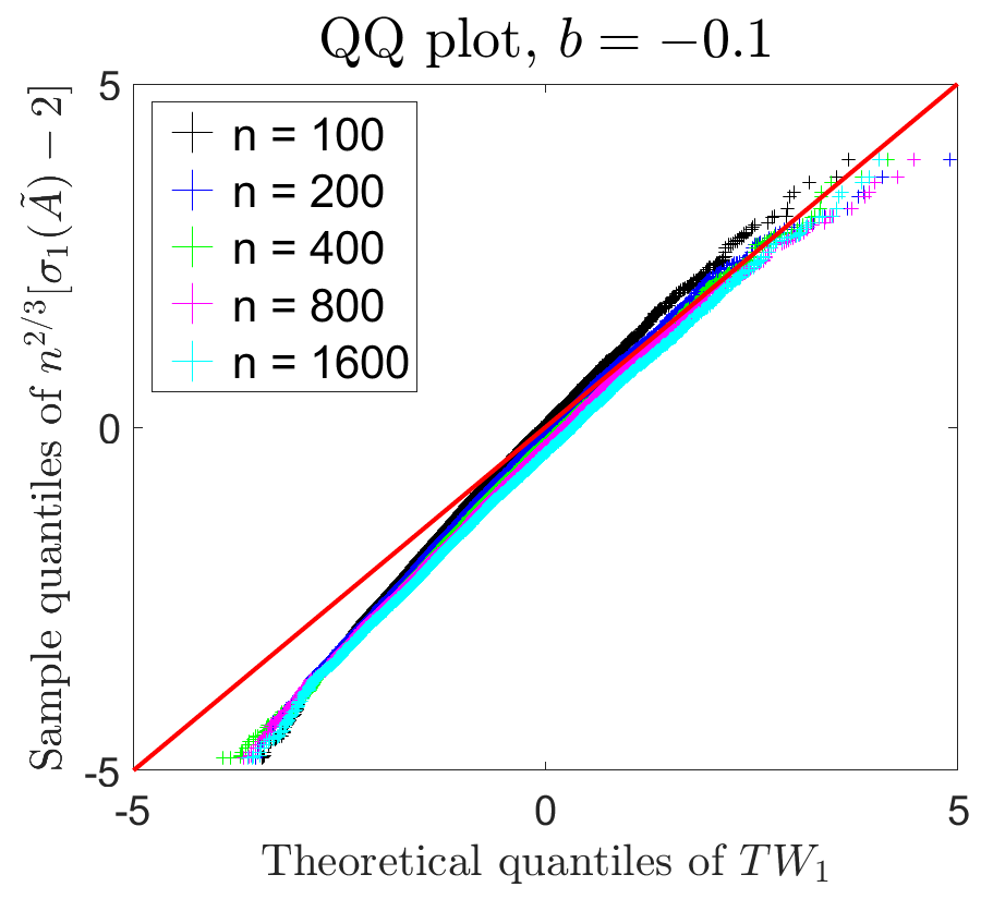
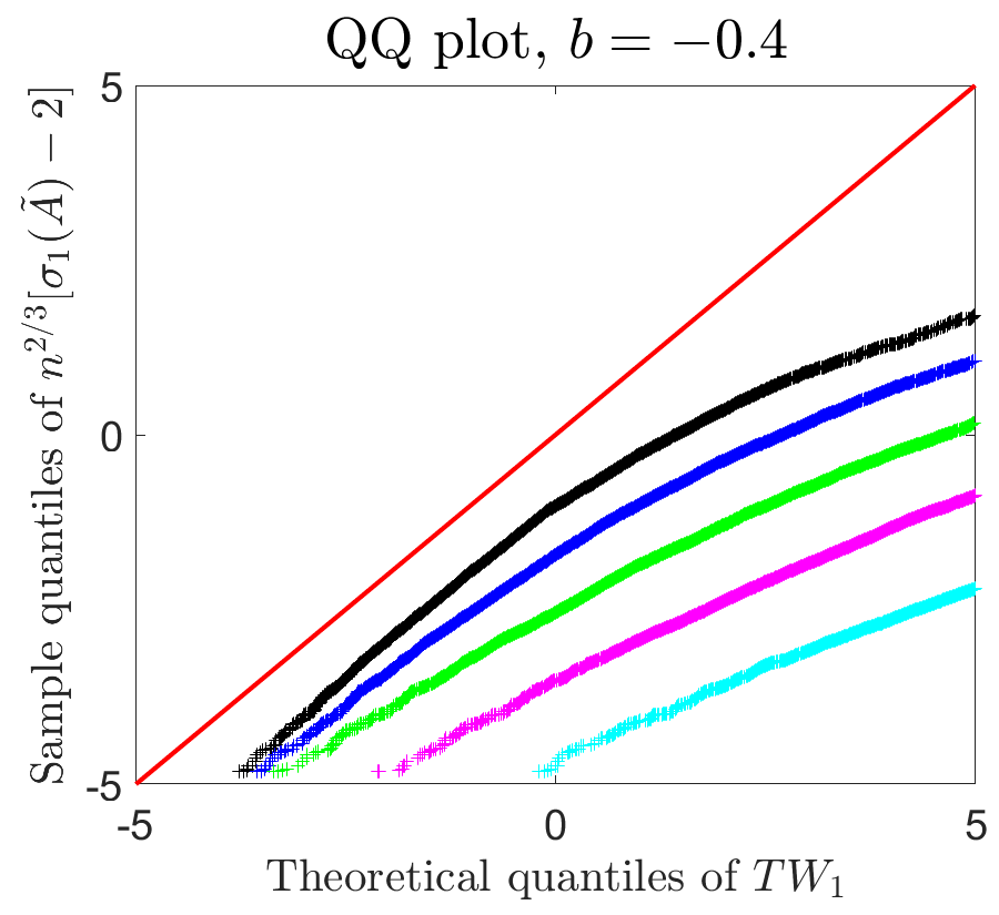
Figure 9: QQ plot of empirical distribution of $T$ using $\widehat{P}$ in (38) vs. ${\rm TW}_{1}$ distribution.

In this paper, we focused exclusively on analyzing network data. We analyzed nodal covariates in data examples, but the covariates do not participate in the network generation model. The consideration is mainly three-fold. First, we pursue a good understanding of a simple model, and then gradually push forward towards more complex ones. Research on the $\beta$-model without covariates still faces several open problems that would require considerable future effort to resolve. Second, the joint modeling approach (Yan et al., 2019; Stein and Leng, 2020, 2021) may encounter substantive challenge in large and sparse networks, where the response is highly extreme imbalanced, with most 0’s and few 1’s. Some treatments may be necessary to properly address this issue, see analogous discussions in classification (Sun et al., 2009). The third consideration is computation. As pointed out by Stein and Leng (2021), the monotonicity lemma would not hold for a joint model involving covariates. Consequently, the joint model could not yet effectively scale up beyond $n\asymp 10^{3}$ nodes. The data examples we studied in this paper have up to $10^{7}$ nodes and are typically very sparse.

Another interesting question is whether our work can be extended to bipartite and directed networks. We believe that the extension to bipartite networks would be quite natural, as Lemma 2 easily extends to the bipartite case, after slight adaptions. Extension to direct networks, however, is nontrivial and would require novel treatment, because there, the lack of symmetry $A_{i,j}\not\equiv A_{j,i}$ breaks Lemma 2. Due to page and scope limits, we will not discuss this in greater detail.

Finally, our paper exclusively focuses on analyzing $\beta$-models with independent edge generation. There exist a line of fine works that address dependent edges (Frank and Strauss, 1986; Hunter et al., 2012; Schweinberger and Stewart, 2020). With the introduction of edge dependency, not only estimation and inference, but even data generation from a given model would become much more difficult and costly. We feel that this is an interesting but also challenging future direction.

Computer code

The computer code, composed by author Meijia Shao, including the full instructions for reproducing the simulation and data analysis results in this paper, is available at https://github.com/MjiaShao/L2-beta-model. It does not include the original code for Chen et al. (2021) and Stein and Leng (2020) that we obtained from Professor Chenlei Leng, and data sets. See its README for more details.

References

- Amazon H2O (2021) Amazon H2O. Amazon H2O AI platform documentation: Generalized Linear Model (GLM). http://h2o-release.s3.amazonaws.com/h2o/rel-jordan/3/docs-website/datascience/glm.html, 2021. Online, Accessed 08-October-2021.
- Babai et al. (1980) László Babai, Paul Erdos, and Stanley M Selkow. Random graph isomorphism. SIaM Journal on computing, 9(3):628–635, 1980.
- Bickel and Chen (2009) Peter J Bickel and Aiyou Chen. A nonparametric view of network models and newman–girvan and other modularities. Proceedings of the National Academy of Sciences, 106(50):21068–21073, 2009.
- Blei et al. (2003) David M Blei, Andrew Y Ng, and Michael I Jordan. Latent dirichlet allocation. the Journal of machine Learning research, 3:993–1022, 2003.
- Chatterjee et al. (2011) Sourav Chatterjee, Persi Diaconis, and Allan Sly. Random graphs with a given degree sequence. The Annals of Applied Probability, 21(4):1400–1435, 2011.
- Chen et al. (2021) Mingli Chen, Kengo Kato, and Chenlei Leng. Analysis of networks via the sparse -model. Journal of the Royal Statistical Society: Series B (Statistical Methodology), 83:887–910, 2021. doi: https://doi.org/10.1111/rssb.12444.
- Chen and Olvera-Cravioto (2013) Ningyuan Chen and Mariana Olvera-Cravioto. Directed random graphs with given degree distributions. Stochastic Systems, 3(1):147–186, 2013.
- Elmer et al. (2020) Timon Elmer, Kieran Mepham, and Christoph Stadtfeld. Students under lockdown: Comparisons of students’ social networks and mental health before and during the covid-19 crisis in switzerland. Plos one, 15(7):e0236337, 2020.
- Erdős et al. (2012) László Erdős, Horng-Tzer Yau, and Jun Yin. Rigidity of eigenvalues of generalized wigner matrices. Advances in Mathematics, 229(3):1435–1515, 2012.
- Fan et al. (2020a) Yifan Fan, Huiming Zhang, and Ting Yan. Asymptotic theory for differentially private generalized -models with parameters increasing. arXiv preprint arXiv:2002.12733, 2020a.
- Fan et al. (2020b) Zhenyu Fan, Liping Chen, Jun Li, Xin Cheng, Jingmao Yang, Cheng Tian, Yajun Zhang, Shaoping Huang, Zhanju Liu, and Jilin Cheng. Clinical features of covid-19-related liver functional abnormality. Clinical Gastroenterology and Hepatology, 18(7):1561–1566, 2020b.
- Fienberg (2012) Stephen E Fienberg. A brief history of statistical models for network analysis and open challenges. Journal of Computational and Graphical Statistics, 21(4):825–839, 2012.
- Frank and Strauss (1986) Ove Frank and David Strauss. Markov graphs. Journal of the american Statistical association, 81(395):832–842, 1986.
- Gao (2020) Wayne Yuan Gao. Nonparametric identification in index models of link formation. Journal of Econometrics, 215(2):399–413, 2020.
- Graham (2017) Bryan S Graham. An econometric model of network formation with degree heterogeneity. Econometrica, 85(4):1033–1063, 2017.
- Hastie et al. (2009) Trevor Hastie, Robert Tibshirani, and Jerome Friedman. The Elements of Statistical Learning. Springer New York, 2009. doi: 10.1007/978-0-387-84858-7. URL https://doi.org/10.1007/978-0-387-84858-7.
- Hillar and Wibisono (2013) Christopher Hillar and Andre Wibisono. Maximum entropy distributions on graphs. arXiv preprint arXiv:1301.3321, 2013.
- Hillar et al. (2012) Christopher J Hillar, Shaowei Lin, and Andre Wibisono. Inverses of symmetric, diagonally dominant positive matrices and applications. arXiv preprint arXiv:1203.6812, 2012.
- Hirsch et al. (2020) Jamie S Hirsch, Jia H Ng, Daniel W Ross, Purva Sharma, Hitesh H Shah, Richard L Barnett, Azzour D Hazzan, Steven Fishbane, Kenar D Jhaveri, Mersema Abate, et al. Acute kidney injury in patients hospitalized with covid-19. Kidney international, 98(1):209–218, 2020.
- Holland and Leinhardt (1981) Paul W Holland and Samuel Leinhardt. An exponential family of probability distributions for directed graphs. Journal of the american Statistical association, 76(373):33–50, 1981.
- Hunter et al. (2012) David R Hunter, Pavel N Krivitsky, and Michael Schweinberger. Computational statistical methods for social network models. Journal of Computational and Graphical Statistics, 21(4):856–882, 2012.
- Karwa and Slavković (2016) Vishesh Karwa and Aleksandra Slavković. Inference using noisy degrees: Differentially private -model and synthetic graphs. The Annals of Statistics, 44(1):87–112, 2016.
- Kulkarni et al. (2020) Ninad Kulkarni, Colby Wise, George Price, and Miguel Romero. Amazon website services (AWS) database blog: Building and querying the AWS COVID-19 knowledge graph. https://aws.amazon.com/cn/blogs/database/building-and-querying-the-aws-covid-19-knowledge-graph/, 2020. Published 01-Jul-2020, accessed 14-Sep-2021.
- Lee and Yin (2014) Ji Oon Lee and Jun Yin. A necessary and sufficient condition for edge universality of wigner matrices. Duke Mathematical Journal, 163(1):117–173, 2014.
- Lee and Courtade (2020) Kuan-Yun Lee and Thomas Courtade. Minimax bounds for generalized linear models. Advances in Neural Information Processing Systems, 33:9372–9382, 2020.
- Lei (2016) Jing Lei. A goodness-of-fit test for stochastic block models. The Annals of Statistics, 44(1):401–424, 2016.
- Li and Yang (2021) Binghui Li and Yuehan Yang. Undirected and directed network analysis of the chinese stock market. Computational Economics, pages 1–19, 2021.
- Li et al. (2015) Yen-Huan Li, Jonathan Scarlett, Pradeep Ravikumar, and Volkan Cevher. Sparsistency ofell_1-regularized m-estimators. In Artificial Intelligence and Statistics, pages 644–652. PMLR, 2015.
- Liu et al. (2019) Hanwen Liu, Huaizhen Kou, Chao Yan, and Lianyong Qi. Link prediction in paper citation network to construct paper correlation graph. EURASIP Journal on Wireless Communications and Networking, 2019(1):1–12, 2019.
- Lu et al. (1997) Jiandong Lu, Daijin Ko, and Ted Chang. The standardized influence matrix and its applications. Journal of the American Statistical Association, 92(440):1572–1580, 1997.
- Lubold et al. (2021) Shane Lubold, Bolun Liu, and Tyler H McCormick. Spectral goodness-of-fit tests for complete and partial network data. arXiv preprint arXiv:2106.09702, 2021.
- McCullagh and Nelder (2019) Peter McCullagh and John A Nelder. Generalized linear models. Routledge, 2019.
- Mukherjee et al. (2018) Rajarshi Mukherjee, Sumit Mukherjee, and Subhabrata Sen. Detection thresholds for the -model on sparse graphs. The Annals of Statistics, 46(3):1288–1317, 2018.
- Park and Newman (2004) Juyong Park and Mark EJ Newman. Statistical mechanics of networks. Physical Review E, 70(6):066117, 2004.
- Pei et al. (2020) Guangchang Pei, Zhiguo Zhang, Jing Peng, Liu Liu, Chunxiu Zhang, Chong Yu, Zufu Ma, Yi Huang, Wei Liu, Ying Yao, et al. Renal involvement and early prognosis in patients with covid-19 pneumonia. Journal of the American Society of Nephrology, 31(6):1157–1165, 2020.
- Rausch (2020) Ilja Rausch. Covid-19: Knowledge graph - a network analysis. https://www.kaggle.com/iljara/covid-19-knowledge-graph-a-network-analysis, 2020. Published 21-May-2020, accessed, 22-Sep-2021.
- Rinaldo et al. (2013) Alessandro Rinaldo, Sonja Petrović, and Stephen E Fienberg. Maximum lilkelihood estimation in the -model. The Annals of Statistics, pages 1085–1110, 2013.
- Schweinberger and Stewart (2020) Michael Schweinberger and Jonathan Stewart. Concentration and consistency results for canonical and curved exponential-family models of random graphs. The Annals of Statistics, 48(1):374–396, 2020.
- Steenwinckel et al. (2020) Bram Steenwinckel, Gilles Vandewiele, Ilja Rausch, Pieter Heyvaert, Pieter Colpaert, Pieter Simoens, Anastasia Dimou, Filip De Turkc, and Femke Ongenae. Facilitating covid-19 meta-analysis through a literature knowledge graph. In Accepted in Proc. of 19th International Semantic Web Conference (ISWC), 2020.
- Stein and Leng (2020) Stefan Stein and Chenlei Leng. A sparse -model with covariates for networks. arXiv preprint arXiv:2010.13604, 2020.
- Stein and Leng (2021) Stefan Stein and Chenlei Leng. A sparse random graph model for sparse directed networks. arXiv preprint arXiv:2108.09504, 2021.
- Su et al. (2018) Liju Su, Xiaodi Qian, and Ting Yan. A note on a network model with degree heterogeneity and homophily. Statistics & Probability Letters, 138:27–30, 2018.
- Sun et al. (2009) Yanmin Sun, Andrew KC Wong, and Mohamed S Kamel. Classification of imbalanced data: A review. International journal of pattern recognition and artificial intelligence, 23(04):687–719, 2009.
- van Wieringen (2015) Wessel N van Wieringen. Lecture notes on ridge regression. arXiv preprint arXiv:1509.09169, 2015.
- Wahlström et al. (2017) Johan Wahlström, Isaac Skog, Patricio S La Rosa, Peter Händel, and Arye Nehorai. The -model—maximum likelihood, cramér–rao bounds, and hypothesis testing. IEEE Transactions on Signal Processing, 65(12):3234–3246, 2017.
- Wise et al. (2020) Colby Wise, Vassilis N Ioannidis, Miguel Romero Calvo, Xiang Song, George Price, Ninad Kulkarni, Ryan Brand, Parminder Bhatia, and George Karypis. Covid-19 knowledge graph: accelerating information retrieval and discovery for scientific literature. arXiv preprint arXiv:2007.12731, 2020.
- Witten et al. (2009) Daniela M Witten, Robert Tibshirani, and Trevor Hastie. A penalized matrix decomposition, with applications to sparse principal components and canonical correlation analysis. Biostatistics, 10(3):515–534, 2009.
- Yan and Xu (2013) Ting Yan and Jinfeng Xu. A central limit theorem in the -model for undirected random graphs with a diverging number of vertices. Biometrika, 100(2):519–524, 2013.
- Yan et al. (2015) Ting Yan, Yunpeng Zhao, and Hong Qin. Asymptotic normality in the maximum entropy models on graphs with an increasing number of parameters. Journal of Multivariate Analysis, 133:61–76, 2015.
- Yan et al. (2016) Ting Yan, Chenlei Leng, and Ji Zhu. Asymptotics in directed exponential random graph models with an increasing bi-degree sequence. The Annals of Statistics, 44(1):31–57, 2016.
- Yan et al. (2019) Ting Yan, Binyan Jiang, Stephen E Fienberg, and Chenlei Leng. Statistical inference in a directed network model with covariates. Journal of the American Statistical Association, 114(526):857–868, 2019.
- Zhang et al. (2020) Chao Zhang, Lei Shi, and Fu-Sheng Wang. Liver injury in covid-19: management and challenges. The lancet Gastroenterology & hepatology, 5(5):428–430, 2020.
- Zhang and Xia (2022) Yuan Zhang and Dong Xia. Edgeworth expansions for network moments. The Annals of Statistics, 50(2):726–753, 2022.
- Zhao et al. (2012) Yunpeng Zhao, Elizaveta Levina, and Ji Zhu. Consistency of community detection in networks under degree-corrected stochastic block models. The Annals of Statistics, 40(4):2266–2292, 2012.