Voting algorithms for unique games on complete graphs

Abstract

An approximation algorithm for a constraint satisfaction problem is called robust if it outputs an assignment satisfying a $(1-f(\epsilon))$-fraction of the constraints on any $(1-\epsilon)$-satisfiable instance, where the loss function $f$ is such that $f(\epsilon)\rightarrow 0$ as $\epsilon\rightarrow 0$. Moreover, the runtime of a robust algorithm should not depend in any way on $\epsilon$. In this paper, we present such an algorithm for Min-Unique-Games$(q)$ on complete graphs with $q$ labels. Specifically, the loss function is $f(\epsilon)=(\epsilon+c_{\epsilon}\epsilon^{2})$, where $c_{\epsilon}$ is a constant depending on $\epsilon$ such that $\lim_{\epsilon\rightarrow 0}c_{\epsilon}=16$. The runtime of our algorithm is $O(qn^{3})$ (with no dependence on $\epsilon$) and can run in time $O(qn^{2})$ using a randomized implementation with a slightly larger constant $c_{\epsilon}$. Our algorithm is combinatorial and uses voting to find an assignment. It can furthermore be used to provide a PTAS for Min-Unique-Games$(q)$ on complete graphs, recovering a result of Karpinski and Schudy with a simpler algorithm and proof. We also prove -hardness for Min-Unique-Games$(q)$ on complete graphs and (using a randomized reduction) even in the case where the constraints form a cyclic permutation, which is also known as Min-Linear-Equations-mod-$q$ on complete graphs.

1 Introduction

As defined by Zwick [Zwi98], an approximation algorithm for a constraint satisfaction problem (CSP) is called robust if it outputs an assignment satisfying a $(1-f(\varepsilon))$-fraction of the constraints on any $(1-\varepsilon)$-satisfiable instance, where the loss function $f$ is such that $f(\varepsilon)\rightarrow 0$ as $\varepsilon\rightarrow 0$. Moreover, the runtime of the algorithm should not depend in any way on $\varepsilon$. Robust algorithms for CSPs have been studied extensively [GZ11, KOT⁺12, BK16, DKK⁺19]. For example, the famous random hyperplane rounding algorithm for the maximum cut problem yields a robust approximation for the complementary minimization problem [GW95] and is essentially optimal [OW08].

Let us call an approximation algorithm super robust if the loss function has the form $f(\varepsilon)=\varepsilon+O(\varepsilon^{2})$. Such super robust algorithms are relevant in the design of approximation algorithms because, as we will discuss later on, if one has a super robust algorithm for the min version of a problem and a polynomial time approximation scheme (PTAS) for the complementary max version, then we can derive a PTAS for the min version as well. Note that the existence of a PTAS does not imply the existence of a super robust algorithm. There is a wide range of techniques to obtain a PTAS for the max versions of various constraint satisfactions problems on dense graphs (see e.g., [AKK99]). In contrast, we are not aware of super robust algorithms for CSPs or similar problems, even on dense graphs.

In this article we investigate super robust approximation algorithms for Unique-Games on complete graphs, which are CSPs. We now define the problems under consideration. Let $G=(V,E)$ be a complete graph with an arbitrary linear order on the vertices, let $q$ be a positive integer (where $q\leq\poly(n)$) and let $[q]=\{0,\ldots,q-1\}$. (Note that $G$ is simple and therefore does not contain any multi-edges or self-loops.) Let $n$ denote the number of vertices and $m$ the number of edges in $G$ (i.e., $n=|V|$ and $m={n\choose 2}$). We use $uv=vu$ to refer to an edge in $E$ and $(u,v)$ to refer to an ordered pair or arc. An assignment is a map $x:V\rightarrow[q]$ giving a label $x_{v}$ to each vertex $v$. For each ordered pair of vertices $(u,v)$ there is a permutation $\pi_{uv}:[q]\rightarrow[q]$. This permutation is interpreted as a constraint as follows: an assignment $x$ satisfies the constraint if $x_{v}=\pi_{uv}(x_{u})$. This is equivalent to the constraint $x_{u}=\pi_{vu}(x_{v})$ since we require $\pi_{vu}=\pi^{-1}_{uv}$. A set of constraints is satisfiable if there exists an assignment satisfying all of them. Then the Min-Unique-Games$(q)$-Full problem is the following.

Problem 1 (Min-Unique-Games$(q)$-Full).

Given a complete graph $G$, a positive integer $q$ and a permutation $\pi_{uv}:[q]\rightarrow[q]$ for each ordered pair of vertices $(u,v)$ with $u<v$ (such that $\pi_{vu}=\pi^{-1}_{uv}$), find a minimum cardinality subset of edges of $G$ whose deletion results in a satisfiable set of constraints.

In a special case of this problem, each permutation is cyclic. Specifically, for each ordered pair of vertices $(u,v)$ there is a given integer $c_{uv}\in[q]$ (symmetrically, $c_{vu}=q-c_{uv}\bmod q$). For each edge $uv\in E$ with $u<v$, there is a constraint $x_{u}-x_{v}\equiv c_{uv}\bmod q$. (Observe that $x_{v}-x_{u}\equiv c_{vu}\bmod q$ is an equivalent constraint.) In general graphs, this problem is also known as Min-Linear-Equations-mod-$q$, which we abbreviate to Min-Lin-Eq$(q)$.

Problem 2 (Min-Lin-Eq$(q)$-Full).

Given a complete graph $G$, a positive integer $q$ and a constraint $x_{u}-x_{v}\equiv c_{uv}\bmod q$ for each ordered pair of vertices $(u,v)$ with $u<v$ (such that $c_{vu}=q-c_{uv}$), find a minimum cardinality subset of edges of $G$ whose deletion results in a satisfiable set of constraints.

We refer to the general versions of Problems 1 and 2 (i.e., when $G$ is not necessarily a complete graph) as Min-Unique-Games$(q)$ and Min-Lin-Eq$(q)$, respectively, and to the complementary versions (i.e., when one aims at maximizing the number of satisfied constraints) as Max-Unique-Games$(q)$ and Max-Lin-Eq$(q)$. Although it might seem like an easier problem, a constant factor approximation for Max-Lin-Eq$(q)$ yields a constant factor approximation for Max-Unique-Games$(q)$ [KKMO07].

Our results.

In this paper, we first present a super robust algorithm for Min-Lin-Eq$(q)$-Full. Specifically, the runtime of our algorithm is $O(qn^{3})$ in the RAM model (with no dependence on $\varepsilon$) and the loss function is $f(\varepsilon)=(\varepsilon+c_{\varepsilon}\varepsilon^{2})$, where $c_{\varepsilon}$ is a constant depending on $\varepsilon$ such that $\lim_{\varepsilon\rightarrow 0}c_{\varepsilon}=16$. A randomized implementation with a slightly larger constant $c_{\varepsilon}$ in the loss function runs in time $O(qn^{2})$. We show that our algorithm can be extended to the so-called everywhere dense case, which is where every vertex has degree at least $(1-\delta)(n-1)$ for some constant density parameter $\delta\in(0,1)$ [AKK99].

Our algorithm is very simple, purely combinatorial and uses voting to find an assignment. First, we find an initial assignment using a pivot algorithm in the spirit of [ACN08], which is a 3-approximation in the case of Min-Lin-Eq$(q)$-Full (Section 2). Then we improve this solution according to “votes” of the other vertices based on their initial assignments (Section 3). We discuss the extension to the dense case, whose details can be found in Appendix B. When the alphabet size is constant, we can couple our robust algorithm with classical approximation algorithms for the complementary problem to obtain a PTAS for Min-Unique-Games$(q)$-Full (and thus Min-Lin-Eq$(q)$-Full). This is explained in Section 4, and recovers a result of Karpinski and Schudy [KS09], with a simpler proof. Recall that given a $(1-\varepsilon)$-satisfiable instance, we can find a $(1+O(\varepsilon))$-approximation via an algorithm whose running time is independent of $\varepsilon$. To obtain such a guarantee via the algorithm of Karpinski and Schudy, we would need to exhaustively search for an assignment on a sample of size $\Omega(1/\varepsilon^{2})$, which leads to a running time of $\Omega(q^{1/\varepsilon^{2}})$. Thus finding an algorithm that skips this exhaustive assignment step typical of a PTAS is the key to obtaining a super robust algorithm.

We also consider the hardness of Min-Unique-Games$(q)$-Full (Section 5). In the case of $q=2$, the -hardness for Min-Lin-Eq$(q)$-Full follows from the NP-hardness of Correlation-Clustering with two clusters (i.e., MinDisAgree[2]) due to Giotis and Guruswami [GG06]. For $q\geq 3$, the hardness of Min-Unique-Games$(q)$-Full does not appear to be explicitly considered anywhere in the literature and thus its complexity status was open. Therefore, we prove -hardness for Min-Unique-Games$(q)$-Full for $q\geq 3$. For Min-Lin-Eq$(q)$-Full, we prove NP-hardness under the weaker assumption that $\NP\subsetneq\BPP$. Our reduction is similar to the hardness reductions for Feedback-Arc-Set-Tournaments [ACN08, Alo06, CTY07] and for fully-dense problems [AA07] but is not directly implied by them since, for example, the latter result only holds for fully-dense CSPs on a binary domain. Both proofs are deferred to Appendix C.

Background on Unique-Games.

Unique-Games is one of the most important problems in approximation algorithms due to its direct connection with the famous Unique Games Conjecture of Khot [Kho02], which has wide-ranging implications in the hardness of approximation. Roughly speaking, the conjecture states that there is no constant-factor approximation algorithm for Max-Unique-Games$(q)$. It is not hard to see that there is an algorithm with approximation factor $1/q$. Many approximation algorithms, which beat this factor, have been developed, although none give constant-factor approximations. Some of these use semidefinite programming (SDP) [Kho02, Tre05, CMM06, Rag08], and some use linear programming (LP) [GT06]. It is known that one can find a constant factor approximation for Max-Unique-Games$(q)$ in subexponential time [ABS15, BRS11, BBK⁺21]. See [Kho10, BS14] for surveys on the Unique Games Conjecture.

Applications.

In addition to its theoretical significance, Unique-Games is closely related to angular synchronization and phase reconstruction problems with applications in many fields including computer vision [ARC06] and optics [Wal63, Mil90, RW01]. The models considered in these applied settings are usually constructed by fixing a satisfiable instance and adding noise from some specified distribution to each constraint [BSA13, BBS17, ZB18, GZ19, IPSV20]. (This corresponds to perturbing each $c_{uv}$.) The goal is exact recovery of the original (satisfiable) instance. Another, more combinatorial, model corresponds more closely to the statement of the Unique-Games problem. In this setting, we begin with a satisfiable instance and for each constraint, with some specified probability, noise from a known distribution is added  [Sin11]. Notice that in this setting, not all constraints are necessarily perturbed. Thus, under certain parameters (e.g., small probability of perturbing a constraint and uniform noise), the solution to the original input instance is the solution to the instance of Unique-Games problem corresponding to the perturbed instance. Both models have been studied on complete graphs [Sin11, GZ19, FKM21]. Since the noise is generated from some particular distribution, the problem instance is not a worst-case or adversarially perturbated instance, and the analysis of the recovery procedures usually requires knowledge of the specific perturbation model. Nevertheless, an algorithm with a worst-case performance guarantee, such as ours, can be applied to instances belonging to this model. In practical settings, the simplicity and implementability of our algorithm are desirable properties.

Previous results.

In terms of a robust algorithm for Min-Unique-Games$(q)$, there is an algorithm based on semidefinite programming with loss function $f(\varepsilon)=\sqrt{\varepsilon\log{q}}$ [CMM06]. This is not really a robust algorithm for Min-Unique-Games$(q)$ since the loss function depends on $q$ and not solely on $\varepsilon$, and $q$ could be a function of $n$. Robust algorithms for Constraint Satisfaction Problems have been studied in depth [GZ11, KOT⁺12, BK16, DKK⁺19]. Min-Unique-Games$(q)$ has also been studied on expanders [AKK⁺08], and this work gives an algorithm with loss function $O(\frac{\varepsilon}{\lambda}\log{\frac{\lambda}{\varepsilon}})$, where $\lambda$ is the second smallest eigenvalue of the normalized Laplacian of the input graph $G$. This algorithm is robust in the case of complete graphs, since $\lambda=1$ for a complete graph. In [GS11], the stated loss function for a graph with $\lambda=1$ is $f(\varepsilon)=(3+\eta)\varepsilon$, which is achieved in time $n^{O(2/\eta)}$. Perhaps a more careful analysis of these algorithms can yield a slightly better loss function in the case of complete graphs. In any case, these loss functions correspond to constant factor approximations and are therefore worse than the one we present in this paper by an order of magnitude, and for example, they cannot be leveraged to obtain a PTAS as in Section 4. Moreover, it is somewhat interesting that our loss function can be achieved using combinatorial methods rather than relying on tools from semidefinite programming as is the case in [AKK⁺08] and on semidefinite hierarchies as in [GS11]. We remark that the Unique Games Conjecture is equivalent to the conjecture that a basic assignment-based semidefinite program is the best tool for solving an instance of Max-Unique-Games$(q)$ [Rag08]. Thus, it is reasonable to consider different algorithmic tools. We note that the algorithm of [AKK⁺08] can be interpreted as a pivot algorithm and we discuss this connection in Section 2.

Min-Unique-Games$(q)$ has also been studied on dense graphs and there is a PTAS with stated runtime $O(n^{2})+2^{O(\frac{1}{\varepsilon})}$ [KS09]. This algorithm, based on a combination of random sampling and voting, is not robust as the runtime depends on $\varepsilon$. Notice that this runtime assumes that both $q$ and the density parameter $\delta$ are fixed (i.e., the dependence on $q$ and $\delta$ occur in the exponent but are not stated explicitly in the runtime).

Finally, we remark that many combinatorial optimization problems have been specifically studied on complete graphs or tournaments. For example, Feedback-Arc-Set-Tournaments has a much better approximation guarantee than is currently known for the general case, but is still -hard [ACN08]. Another well-studied example is the special case of Correlation-Clustering known as MinDisagree on complete graphs [BBC04, CGW05, GG06, ACN08, CMSY15]. The latter problem is APX-hard [CGW05], so it is unlikely to have a super robust approximation (see Section 4). Although Feedback-Arc-Set-Tournaments has a PTAS [KMS07], it also does not seem to have a known super robust approximation algorithm.

2 Pivot Algorithm for Min-Lin-Eq$(q)$-Full

In a given instance of Min-Lin-Eq$(q)$-Full on a graph $G$, each cycle in $G$ is either consistent or inconsistent. A cycle is consistent (inconsistent) if it is satisfiable (unsatisfiable, respectively). Observe that a feasible solution to Problem 2 is a hitting set for the set of inconsistent cycles. The following algorithm outputs a vertex labeling such that the unsatisfied edges form a hitting set for the inconsistent cycles.

Pivot Algorithm Input: An instance of Min-Lin-Eq$(q)$-Full on a graph $G=(V,E)$. 1. Pick a pivot $p\in V$ uniformly at random and label $p$ with 0. 2. For each vertex $v\in V\setminus{p}$, assign $v$ label corresponding to the constraint on edge $pv$. (Specifically, $\ell(v)=c_{vp}$.)

On an input for Min-Unique-Games$(q)$-Full, the algorithm can be modified to test each possible label in $[q]$ for the pivot chosen in Step 1.

Theorem 2.1.

The Pivot Algorithm is a $3$-approximation algorithm for Problem 2.

The proof of Theorem 2.1 follows almost directly from the analysis of the KwikSort Algorithm for Feedback-Arc-Set-Tournaments [ACN08]. For completeness, the proof can be found in Appendix A. We also give an example showing that this analysis is tight. We remark that for a satisfiable instance of Unique-Games, one can choose any spanning tree and “propagate” the values along the spanning tree, resulting in an optimal solution. The pivot algorithm is also a type of spanning-tree algorithm, since it determines the assignments by using the edges incident to the pivot, which form a star-shaped spanning-tree.

2.1 Pivot Algorithm and SDP Rounding

In [AKK⁺08], they first solve a semidefinite program and then they use its solution to produce a new set of permutations $\{\sigma_{uv}\}$ for each edge $uv\in E$. Suppose that initial instance (on which the SDP is solved) is on a complete graph and is $(1-\varepsilon)$-satisfiable. If the new instance (using the $\sigma$-permutations) is also $(1-\varepsilon)$-satisfiable (e.g., if $\sigma_{uv}=\pi_{uv}$ for every edge), then their algorithm produces the same output as the Pivot Algorithm and the loss function $f(\varepsilon)=3\varepsilon$. The analysis used in [AKK⁺08] does not seem sufficient to show that the new instance on the $\sigma$-permutations is actually a $(1-\varepsilon^{\prime})$-satisfiable instance for some $\varepsilon^{\prime}<\varepsilon$. Thus, it seems that new analysis or modifications of the algorithm is necessary to obtain an improved loss function.

3 The Voting Algorithm

In this section we present the voting algorithm for Min-Lin-Eq$(q)$-Full, and show that this algorithm is a super robust approximation algorithm for Min-Lin-Eq$(q)$-Full. The idea is to begin with the pivot algorithm from the previous section and use the resulting labels as “temporary” labels. Then, we “correct” this labeling: each vertex (except the pivot) casts a “vote” for the label of every other vertex according to the relevant constraint. The votes are tallied for each vertex by a plurality rule: the final label of a vertex is one that occurs most often in the list of its votes. The algorithm, which we call the Voting Algorithm is presented formally in Section 3.1. The runtime of the Voting Algorithm is $O(n^{3})$. In Section 3.2, we present an algorithm that is equivalent to the Voting Algorithm in that it produces the same output assignment. In Section 3.3, we present a randomized version of the Voting Algorithm with running time $O(n^{2})$ and a slightly worse approximation guarantee.

3.1 The Voting Algorithm for Min-Lin-Eq$(q)$-Full

Voting Algorithm Input: An instance of Min-Lin-Eq$(q)$-Full. 1. Pick a pivot $p\in V$. Label $p$ with $0$ and label each vertex $v\in V$ with temporary label $\operatorname{TEMP}(v)$, which is chosen according to the constraint on edge $(p,v)$. (Specifically, $\operatorname{TEMP}(v)=c_{vp}$.) 2. For each vertex $v$, each neighboring vertex $u\neq p$ votes for a label for $v$, where $u$’s vote is based on its temporary label $\operatorname{TEMP}(u)$. (Specifically, the vote of $u$ for $v$ is $(c_{vu}+\operatorname{TEMP}(u))\bmod q$.) 3. Then each $v$ is assigned a final label $\operatorname{FINAL}(v)$ according to the outcome of its $n-2$ votes (with a plurality rule). Ties are resolved arbitrarily. 4. Output the best $\operatorname{FINAL}$ solution over all choices of $p$ in Step 1.

Notice that for technical reasons, we do not let the pivot $p$ vote in Step 2.

Theorem 3.1.

On a $(1-\varepsilon)$-satisfiable instance of Min-Lin-Eq$(q)$-Full, for $0\leq\varepsilon<\frac{1}{2}$, the Voting Algorithm returns a solution with at most $(\varepsilon+c_{\varepsilon}\varepsilon^{2})m$ unsatisfied constraints where $\lim_{\varepsilon\to 0}c_{\varepsilon}=16$.

An intuition of the proof is as follows. After Step 2., it is easy to see that an assignment is obtained where an $\varepsilon$ fraction of the vertices are incorrect (compared to the optimal solution). This does not ensure that a small enough fraction of the edges are incorrect (i.e., unsatisfied), which is our goal. Therefore, we add the voting step in Step 3., which drastically reduces the number of unsatisfied edges towards our stated goal. This works because in order for a vote to produce a wrong assignment at a vertex, there needs to be a sizable number of either incorrect voters or incorrect adjacent edges, which we can control using a simple charging scheme.

We prove Theorem 3.1 via the following lemma.

Lemma 3.2.

The Voting Algorithm returns a solution with at most $(\varepsilon+2\varepsilon^{2}\nu(2+\nu)+o(1))m$ unsatisfied constraints, where $\nu=2/(1-2\varepsilon)$.

Fix an optimal solution $\operatorname{OPT}$ and denote by $\operatorname{OPT}(v)$ the label it gives to a vertex $v$. In this fixed optimal solution, there are satisfied edges, which we call green edges and unsatisfied edges, which we call red edges.

Since $\varepsilon=\operatorname{OPT_{val}}/m$, the number of red edges incident to $p$ is at most $\varepsilon(n-1)$ for some choice of $p$. We analyze the voting algorithm for this choice of $p$. Without loss of generality, we assume that $\operatorname{OPT}(p)=0$. This means that at least $(1-\varepsilon)(n-1)$ vertices have $\operatorname{TEMP}(u)=\operatorname{OPT}(u)$; we call these good vertices (i.e., incident to green edges), while the other ones are rogue vertices (i.e., incident to red edges). See Figure 1 for an illustration.

Figure 1: Green and red edges are those satisfied and unsatisfied, respectively, in $\operatorname{OPT}$. Green and red vertices are good vertices and rogue vertices, respectively.

The plan is to analyze how much the outcome of the voting algorithm differs from $\operatorname{OPT}$. A vertex is flipped if $\operatorname{FINAL}(v)\neq\operatorname{OPT}(v)$. For a vertex to be flipped, it must be badly influenced by its neighbors. Let $\delta(v)\subset E$ denote the edges incident to vertex $v$. Observe that all good vertices adjacent to $v$ via a green edge in $\delta(v)$ vote correctly with respect to vertex $v$ (i.e., they vote for label $\operatorname{OPT}(v)$).

The two types of vertices that can vote incorrectly for $v$’s label (i.e., they might not vote for label $\operatorname{OPT}(v)$) are (i) rogue vertices incident to green edges in $\delta(v)$, and (ii) vertices incident to red edges in $\delta(v)$. The number of vertices falling into the first category is at most the number of rogue vertices (i.e., at most $\varepsilon(n-1)$). The number of vertices falling into the second category is at most the number of red edges incident to $v$. Hence we say that a vertex $v$ is flippable if the number of red edges incident to $v$ is at least $(n-1)/2-\varepsilon(n-1)$.

Lemma 3.3.

If a vertex $v$ is not flippable, it is not flipped (i.e., $\operatorname{FINAL}(v)=\operatorname{OPT}(v)$).

Proof.

A non-flippable vertex $v$ has at least $(n-1)/2+\varepsilon(n-1)+1$ incident green edges (since by definition the number of incident red edges is at most $(n-1)/2-\varepsilon(n-1)-1$). At least $(n-1)/2+1$ of these edges are incident to good vertices. (Recall a vertex $u$ is good if $\operatorname{TEMP}(u)=\operatorname{OPT}(u)$.) Thus all of these good vertices vote for $v$ to be labeled $\operatorname{OPT}(v)$, and they will win the vote since they form an absolute majority. ∎

Lemma 3.4.

There are at most $\varepsilon\nu n$ flippable vertices.

Proof.

By definition, there are $\operatorname{OPT_{val}}=\varepsilon m$ red edges. Denote by $f$ the number of flippable vertices. Summing the red degree around each flippable vertex gives $f\cdot((n-1)/2-\varepsilon(n-1))\leq 2\varepsilon m$ implying the lemma. ∎

At the end of the algorithm (i.e., according to the labels $\{\operatorname{FINAL}(v)\}$), if an edge is unsatisfied, then either it is red, or it is green and at least one of its endpoints got flipped. In the latter case, we charge that edge positively to (one of) the endpoint(s) that got flipped. Similarly, if an edge is satisfied, then either it is green, or it is red and at least one of its endpoints got flipped. In the latter case, we charge that edge negatively to (one of) the endpoint(s) that got flipped.

Lemma 3.5.

The charges on a flipped vertex $v$ at the end of the algorithm are at most $2\varepsilon(n-1)+\varepsilon\nu n$.

Proof.

For a given vertex $v$, each neighbor $u$ votes for vertex $v$ to have the label $vote(u\rightarrow v)$, where $vote(u\rightarrow v)$ is equal to $\operatorname{TEMP}(u)$ modified according to the constraint on the edge $uv$. A coalition is a maximal set of neighboring vertices $C$ adjacent to $v$ that vote unanimously: for all $u\in C$, $vote(u\rightarrow v)$ has the same value. All the vertices adjacent to $v$ get partitioned into coalitions, and the winning coalition is one with the largest cardinality.

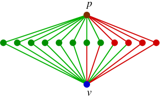
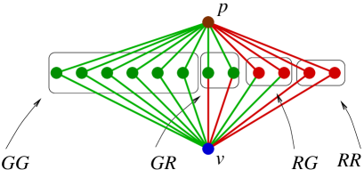
Figure 2: There are $n-2$ vertices that vote for the label of $v$. They are partitioned into four sets: $GG$ are good vertices incident to green edges in $\delta(v)$; $GR$ are good vertices incident to red edges in $\delta(v)$; $RG$ are rogue vertices incident to green edges in $\delta(v)$; $RR$ are rogue vertices incident to red edges in $\delta(v)$.

A flippable vertex $v$ gets flipped if the winning coalition $C_{WIN}$ is not the coalition $C_{OPT}$ (where $C_{OPT}$ is the coalition that votes for $\operatorname{OPT}(v)$). Observe that $C_{OPT}$ contains the subset of good vertices that are incident to green edges in $\delta(v)$. Call this subset $GG$. (See Figure 2.) The winning coalition $C_{WIN}$ is formed of good vertices incident to red edges in $\delta(v)$ (call this subset $W_{GR}$), rogue vertices incident to green edges in $\delta(v)$ (call this subset $W_{RG}$), and rogue vertices incident to red edges in $\delta(v)$ (call this subset $W_{RR}$). (Observe that $W_{GR}\subseteq GR,W_{RG}\subseteq RG$ and $W_{RR}\subseteq RR$. Moreover, note that there might be some vertices in $V\setminus{\{p,v\}}$ that belong to neither $C_{OPT}$ nor to $C_{WIN}$.)

Since the winning coalition wins the vote, $|C_{OPT}|\leq|C_{WIN}|$. Thus,

$$|GG|\leq|W_{GR}|+|W_{RG}|+|W_{RR}|\leq|W_{GR}|+\varepsilon(n-1).$$

The positive charges are upper bounded by $|GG|+|RG|$. (This is not an equality as these edges might end up satisfied if their other endpoint is flipped as well.) The negative charges are at least $|W_{GR}|$ minus those whose other endpoint has been flipped as well. For the other endpoint to be flipped, it needs to be flippable, so the total number of negative charges is at least $|W_{GR}|-\varepsilon\nu n$.

So the total charge is at most:

$$|GG|+|RG|-(|W_{GR}|-\varepsilon\nu n) \leq |W_{GR}|+\varepsilon(n-1)+|RG|-|W_{GR}|+\varepsilon\nu n$$

$$= \varepsilon(n-1)+|RG|+\varepsilon\nu n$$

$$\leq 2\varepsilon(n-1)+\varepsilon\nu n,$$

where we used the fact that $RG$ is a subset of the rogue vertices and therefore has cardinality at most $\varepsilon(n-1)$. ∎

Denote by $\operatorname{VAL}$ the number of unsatisfied edges at the end of the algorithm.

Lemma 3.6.

$\operatorname{VAL}-\operatorname{OPT_{val}}\leq(1+o(1))\cdot\operatorname{OPT_{val}}\cdot 2\varepsilon\nu(2+\nu)$.

Proof.

This difference is exactly the number of green edges (i.e., satisfied in $\operatorname{OPT}$) which become unsatisfied in $\operatorname{VAL}$ minus the number of red edges (i.e., unsatisfied in $\operatorname{OPT}$) which become satisfied in $\operatorname{VAL}$. This difference is exactly controlled by the charging scheme. Combining with Lemmas 3.4 and 3.5, the sum of all charges is at most

$$\varepsilon\nu n(2\varepsilon(n-1)+\varepsilon\nu n) =2\varepsilon^{2}\nu n(n-1)+\varepsilon^{2}\nu^{2}n^{2}$$

$$=2\nu\varepsilon^{2}\frac{n(n-1)}{2}(2+\nu\frac{n}{n-1})$$

$$=\varepsilon\frac{n(n-1)}{2}(4\nu\varepsilon+2\nu^{2}\varepsilon\frac{n}{n-1})$$

$$=\operatorname{OPT_{val}}\cdot 2\varepsilon\nu(2+\nu(1+\frac{1}{n-1}))$$

$$\leq\operatorname{OPT_{val}}\cdot 2\varepsilon\nu(2+\nu)\cdot(1+\frac{1}{n-1}).$$

∎

We note that Lemma 3.2 is implied by Lemma 3.6.

3.2 Equivalent Implementation of Voting Algorithm

We now give an equivalent interpretation of the Voting Algorithm. Recall that $G=(V,E)$ is a simple, complete graph. We define the multigraph ${G^{2}_{mult}}$ to be a graph that contains $n-2$ edges connecting $u$ and $v$, each edge corresponding to a path $uwv$ for $w\in V\setminus{\{u,v\}}$. Each new edge corresponding to a path $uwv$ inherits a $c_{uv}$ value from this path (i.e., $c_{uv}=(c_{uw}+c_{wv})\bmod q$). Now we create a simple, complete graph ${G^{2}_{\star}}$ on the vertex set $V$ in which the edge label $c_{uv}$ for edge $uv$ is determined by taking the most popular $c_{uv}$ value from the $n-2$ values in ${G^{2}_{mult}}$ (ties broken arbitrarily). Notice that it takes $O(n^{3})$ time to construct the instance ${G^{2}_{\star}}$ of Min-Lin-Eq$(q)$-Full, since it takes $O(n)$ time to compute the constraint value on an edge.

Now we can run the Pivot Algorithm from Section 2 on the input instance ${G^{2}_{\star}}$, which takes $O(n)$ time to output an assignment and takes $O(n^{2})$ time if try every vertex as a pivot. Notice that the best output of the Pivot Algorithm on ${G^{2}_{\star}}$ (over all pivots) is the same as the output of the Voting Algorithm on $G$.

3.3 A Faster Randomized Voting Algorithm

Instead of trying all vertices to be the pivot in Step 1. of the Voting Algorithm, we simply choose a single pivot uniformly at random. We refer to this as the Randomized Voting Algorithm.

If we choose a vertex $v$ at random, by Markov’s Inequality, it has probability at least $1/2$ of being incident to at most $2\varepsilon n$ red edges in a fixed optimal solution. Thus, we execute the analysis used in Section 3 replacing $\varepsilon$ with $2\varepsilon$ which leads to the following theorem.

Theorem 3.7.

On a $(1-\varepsilon)$-satisfiable instance of Min-Lin-Eq$(q)$-Full, for $0\leq\varepsilon<\frac{1}{2}$, with probability at least $1/2$, the Randomized Voting Algorithm returns a solution with at most $(\varepsilon+c_{\varepsilon}\varepsilon^{2})m$ unsatisfied constraints where $\lim_{\varepsilon\to 0}c_{\varepsilon}=32$.

3.4 Extension to Min-Unique-Games$(q)$-Full

In the more general setting of Min-Unique-Games$(q)$-Full, we cannot assume that for any vertex $v$ there is an optimal solution that assigns the label $0$ to $v$. We modify the Voting Algorithm from Section 3 slightly to take this into account and obtain the following result, which differs from the case of Min-Lin-Eq$(q)$-Full (i.e., Theorem 3.1) only in the runtime.

Theorem 3.8.

On a $(1-\varepsilon)$-satisfiable instance of Min-Unique-Games$(q)$-Full, for $0\leq\varepsilon<\frac{1}{2}$, the Voting Algorithm returns a solution with at most $(\varepsilon+c_{\varepsilon}\varepsilon^{2})m$ unsatisfied constraints where $\lim_{\varepsilon\to 0}c_{\varepsilon}=16$. The runtime of the algorithm is $O(qn^{3})$.

The only necessary modification of the Voting Algorithm is in Step 1. For each label $\ell\in[q]$ and each pivot choice $p$, the algorithm assigns label $\ell$ to $p$ and then computes the $\operatorname{TEMP}$ and $\operatorname{FINAL}$ labels as before (see Steps 1.–3. of the Voting Algorithm). The algorithm returns the $\operatorname{FINAL}$ labels with the fewest violated constraints. Thus, the runtime is multiplied by a factor of $q$. The analysis of the modified voting algorithm is identical to the analysis presented in Section 3, once we fix a pivot $p$ with label $\ell$, such that the number of red edges incident to $p$ is at most $\varepsilon(n-1)$.

3.5 Extension to Everywhere-Dense Case

For a graph $G=(V,E)$, let $d(v)$ denote the degree of a vertex $v$. Following [AKK99], we define an everywhere $(1-\delta)$-dense graph $G=(V,E)$ to be a graph in which $d(v)\geq(1-\delta)(n-1)$ for each vertex $v\in V$. We can extend the Voting Algorithm to this case. The algorithm is slightly modified.

Voting Algorithm for Everywhere-Dense Graph Input: An instance of Min-Lin-Eq$(q)$ on a $(1-\delta)$-everywhere dense graph $G=(V,E)$. 1. Pick a pivot $p\in V$. Label $p$ with $0$, and label each vertex $v\in V$ adjacent to $p$ with temporary label $\operatorname{TEMP}(v)$, which is chosen according to the constraint on edge $(p,v)$. (Specifically, $\operatorname{TEMP}(v)=c_{vp}$.) 2. For each vertex $v$, each neighboring vertex $u$ with a $\operatorname{TEMP}$ label votes for a label for $v$, where $u$’s vote is based on its temporary label $\operatorname{TEMP}(u)$. (Specifically, the vote of $u$ for $v$ is $(c_{vu}+\operatorname{TEMP}(u))\bmod q$.) 3. Then each $v$ is assigned a final label $\operatorname{FINAL}(v)$ according to the outcome of the votes it received (with a plurality rule). Ties are resolved arbitrarily. 4. Output the best solution over all choices of $p$ in Step 1.

Notice that in contrast to the Voting Algorithm on a complete graph, $p$ also votes in Step 2. The algorithm would also work if $p$ does not vote, but the analysis turns out to be cleaner if $p$ votes.

Let $\operatorname{OPT_{val}}$ denote the value of an optimal solution (i.e., the minimum number of unsatisfied constraints) and let $\operatorname{OPT_{val}}=\varepsilon m$ (i.e., $\varepsilon=\operatorname{OPT_{val}}/m$). The proof of Theorem 3.9 is very similar to that of Theorem 3.1 and the details can be found in Appendix B.

Theorem 3.9.

On a $(1-\varepsilon)$-satisfiable, $(1-\delta)$-everywhere-dense instance of Min-Unique-Games$(q)$, for $0\leq\varepsilon<\frac{1}{2}$, the Voting Algorithm returns a solution with at most $m(\varepsilon+c_{\varepsilon}\varepsilon^{2})/(1-\delta)$ unsatisfied constraints where $\lim_{\varepsilon\to 0}c_{\varepsilon}=16$. The runtime of the algorithm is $O(qn^{3})$.

4 PTAS

The Voting Algorithm from Section 3 provides a good approximation to Min-Unique-Games$(q)$-Full when the value of an optimal solution is small. In the opposing regime, when the value of an optimal solution is large, we can obtain a good approximation for this solution by solving approximately the complementary problem Max-Unique-Games$(q)$-Full, which is the problem of maximizing the number of satisfied constraints. This complementary problem is the maximization version of a Constraint Satisfaction Problem, and, when the alphabet size is constant, those admit very efficient approximation algorithms on dense graphs using sampling techniques, and thus also on complete graphs.

In order to obtain a (randomized) polynomial-time approximation scheme (PTAS) for Min-Unique-Games$(q)$-Full we rely on the following theorem, where we emphasize that $q$ is considered a constant (i.e., the $O(\cdot)$ notation hides an unspecified dependency on $q$). Note that the algorithm underlying this theorem (e.g., in [MS08]) is a very simple greedy algorithm (but the analysis is not that simple).

Theorem 4.1 ([KS09, Theorem 7]).

For any Max-$2$-CSP and any $\tau>0$ there is a randomized algorithm which returns an assignment of cost at least $OPT-\tau n^{2}$ in runtime $O(n^{2})+2^{O(1/\tau^{2})}$.

A MAX-$2$-CSP is a CSP where each constraint involves two variables. When the alphabet size is not constant, a general purpose PTAS for Max-CSPs on complete graphs is ruled out under Gap-ETH, see Romero, Wrochna and Živný [RWŽ21, Corollary E.5]. Whether a PTAS exists for Max-Unique-Games$(q)$-Full when the alphabet size is not constant seems to be open.

Our PTAS is then as follows.

Theorem 4.2.

When the alphabet size $q$ is constant, for any $\tau>0$, we can compute a $(1+\tau)$-approximation for the problem Min-Unique-Games$(q)$-Full in time $O(n^{3})+2^{O(1/\tau^{4})}$.

Note that the runtime in Theorem 4.2 is $O(n^{2})+2^{O(1/\tau^{4})}$ if we use the Randomized Voting Algorithm. This is similar to a result of Karpinsky and Schudy [KS09], with a simpler algorithm.

Proof of Theorem 4.2.

Let $OPT$ denote the optimal value of the problem. If $2\nu(2+\nu)(OPT/m)<\tau$, where $\nu=2/(1-2OPT/m)$, then by Lemma 3.2 we get the needed approximation. Otherwise, since $\nu\geq 2$, we have $OPT\geq\tau m/16$, and thus $m\leq 16OPT/\tau$.

In this case, we compute a $\tau^{\prime}$-approximation to the complementary problem using Theorem 4.1, for $\tau^{\prime}=\tau^{2}/32$. This provides us with a solution where the number of satisfied edges is at least $(m-OPT)-\tau^{\prime}n^{2}$, and thus the number of unsatisfied edges is at most $OPT+\tau^{\prime}n^{2}\leq OPT+32\tau^{\prime}OPT/\tau\leq OPT(1+\tau)$.∎

The argument in the proof of Theorem 4.2 can be generalized as follows.

Observation 4.3.

Let Min-CSP denote a constraint satisfaction problem where the objective is to minimize the number of violated constraints, while Max-Comp-CSP denotes the complementary problem of maximizing the number of satisfied constraints. If there exists a PTAS for Max-Comp-CSP and a super robust algorithm for Min-CSP, then there exists a PTAS for Min-CSP.

Proof.

As in the previous proof, we use one algorithm or the other depending on $OPT$, the optimal value of Min-CSP. We denote by $C$ the number of constraints and write $\varepsilon=OPT/C$.

We fix any $\tau>0$, and if $\varepsilon<\tau$, then a super robust algorithm computes a solution of value $(\varepsilon+O(\varepsilon^{2}))C\leq OPT(1+O(\tau))$, i.e., up to rescaling $\tau$ by a constant factor we get the required approximation guarantee. Otherwise, we have $\tau\leq\varepsilon$, and running the PTAS for Max-Comp-CSP with a target approximation factor of $\tau^{\prime}=\tau^{2}$ yields a solution of value at least $(C-OPT)(1-\tau^{2})$, and thus the number of unsatisfied constraints is at most $OPT+C\tau^{2}\leq OPT+C\tau OPT/C\leq OPT(1+\tau)$. ∎

As a corollary of this observation, since the special case of Correlation Clustering known as MinDisagree on complete graphs is APX-hard and its complementary max version admits a PTAS [BBC04], it is very unlikely to admit a super robust algorithm.

5 -Hardness

In this section we prove the following hardness results. First, we prove standard -hardness for the more general problem of Min-Unique-Games$(q)$-Full. The proof for this theorem is similar in spirit to the hardness reductions of MinDisAgree[$k$] by Giotis and Guruswami [GG06].

Theorem 5.1.

Min-Lin-Eq$(q)$-Full is -hard for $q=2$, and Min-Unique-Games$(q)$-Full is -hard for any value of $q$.

While we do expect Min-Lin-Eq$(q)$-Full to be -hard for values of $q\geq 3$, this does not seem to follow from these proof techniques, which leverage the use of non-cyclic permutations. Theorem 5.2 provides a hardness proof for Min-Lin-Eq$(q)$-Full using randomized reductions. Notice that Theorems 5.1 and 5.2 are incomparable.

Theorem 5.2.

Unless $\NP\subseteq\BPP$, Min-Lin-Eq$(q)$-Full has no polynomial-time algorithm.

To prove Theorem 5.2, we follow the general approach used for Feedback-Arc-Set-Tournament in [ACN08, Alo06, CTY07] and for fully-dense CSPs on a binary domain [AA07]. The proofs of both Theorem 5.1 and Theorem 5.2 are deferred to Appendix C.

Appendix A Analysis of Pivot Algorithm

In a given instance of Min-Lin-Eq$(q)$-Full on a graph $G=(V,E)$, each cycle in $G$ is either consistent or inconsistent. Let ${\mathcal{I}}$ denote the set of inconsistent cycles and let ${\mathcal{T}}\subseteq{\mathcal{I}}$ denote the set of inconsistent triangles in $G$. Observe that a feasible solution to Problem 2 is a hitting set for the set of inconsistent cycles. Consider the following linear programming relaxation of Problem 2 and its dual.

$$\min\sum_{e\in E} x_{e}$$

$$\sum_{e\in C}x_{e} \geq 1\text{ for all cycles }C\in{\mathcal{I}},$$

$$x_{e} \geq 0. P_{UG}$$ ()

$$\max\sum_{C\in{\mathcal{I}}} y_{C}$$

$$\sum_{C\in{\mathcal{I}}:e\in C}y_{C} \leq 1\text{ for all }e\in E,$$

$$y_{C} \geq 0. D_{UG}$$ ()

Claim A.1.

Any fractional packing of inconsistent triangles in $G$ is a lower bound on the optimal value of $P_{UG}$.

Proof..

The optimal value of $P_{UG}$ is lower bounded by a fractional packing of inconsistent cycles (i.e., a feasible solution for $D_{UG}$). A fractional packing of inconsistent triangles is a lower bound on a fractional packing of inconsistent cycles. $\Diamond$

See 2.1

Proof.

The Pivot Algorithm assigns a label $\ell(v)\in[q]$ to each $v\in V$. Each edge $uv\in E$ whose constraint is unsatisfied by the labels $\ell(u)$ and $\ell(v)$ is added to the “deletion set” $F\subset E$. Let $G^{\prime}$ be the graph consisting of the remaining edges (i.e., $G^{\prime}=(V,E\setminus{F})$). The following claim follows directly from the definition of $G^{\prime}$.

Claim A.2.

$G^{\prime}$ contains no inconsistent cycles.

Let $t=\{i,j,k\}$ be an inconsistent triangle in $G$ and let $A_{t}$ denote the event that $p\in\{i,j,k\}$. Let $p_{t}$ be the probability of event $A_{t}$. Then,

$$\mathbbm{E}[\text{Number of deleted edges}] = \sum_{t\in{\mathcal{T}}}p_{t}.$$ (1)

Claim A.3.

Setting $y^{\prime}_{C}=y^{\prime}_{t}=\frac{p_{t}}{3}$ if $C=t\in{\mathcal{T}}$ and $y^{\prime}_{C}=0$ otherwise is dual feasible.

Proof..

Let $B_{e}$ be the event that edge $e$ was deleted by the algorithm. Let $B_{e}\wedge A_{t}$ be the event that edge $e$ was deleted due to $A_{t}$. Given event $A_{t}$, each edge in $t$ is equally likely to be deleted. So we have

$$Pr(B_{e}\wedge A_{t}) =Pr(B_{e}|A_{t})Pr(A_{t})$$

$$=\frac{1}{3}\times p_{t}$$

$$=\frac{p_{t}}{3}.$$

Note that for any $t\neq t^{\prime}\in{\mathcal{T}}$ such that $e\in t$ and $e\in t^{\prime}$, $B_{e}\wedge A_{t}$ and $B_{e}\wedge A_{t^{\prime}}$ are disjoint events. Hence, $\underset{t:e\in t}{\sum}\Pr(B_{e}\wedge A_{t})\leq 1$. This implies that, for all $e\in E$:

$$\sum_{C:e\in C}y^{\prime}_{C}=\sum_{t:e\in t}\frac{p_{t}}{3}\leq 1.$$

We can therefore conclude that $\{y^{\prime}_{C}\}$ is a dual-feasible solution. $\Diamond$

From Claim A.3 and (1), we can conclude that the pivot algorithm has an approximation ratio of $3$. ∎

To derandomize the pivot algorithm, observe that we can run the algorithm $n$ times, each time choosing a different vertex as pivot. Consider some fixed optimal solution $\operatorname{OPT}$ that violates exactly $\varepsilon{n\choose 2}=\varepsilon m=\operatorname{OPT_{val}}$ constraints. For some choice of pivot, the number of labels the algorithm incorrectly assigns is at most $\varepsilon(n-1)$. Since each of these vertices is incident to at most $(n-1)$ edges, the total number of incorrect edges is at most

$$\varepsilon m+\varepsilon(n-1)^{2}\leq 3\varepsilon m=3\cdot\operatorname{OPT_{val}}.$$

A.1 Tight example

We can show that the analysis yielding a 3-approximation ratio is tight. Imagine that we have a complete graph such that all edges except those in a Hamilton cycle are associated with the constraint $x_{u}-x_{v}\equiv 0\bmod q$. The edges in the Hamilton cycle are associated with the constraint $x_{u}-x_{v}\equiv 1\bmod q$. Notice that all pivots lead to the same number constraints being (un)satisfied. An optimal solution can satisfy ${n\choose 2}-n$ constraints and leaves $n$ constraints unsatisfied. Let $p$ be the pivot and let $p-1$ and $p+1$ be its two neighbors on the Hamilton cycle. Then the following edges are unsatisfied:

1. The $n-4$ edges in the Hamilton cycle with neither endpoint in $\{p-1,p,p+1\}$.

2. The $n-4$ edges not in the Hamilton cycle with endpoint $p-1$.

3. The $n-4$ edges not in the Hamilton cycle with endpoint $p+1$.

So, asymptotically, we have $3n$ unsatisfied edges, while an optimal solution leaves only $n$ edges unsatisfied.

Appendix B Analysis of Voting Algorithm in Everywhere-Dense Case

In this section, we prove the following theorem. See 3.9

For convenience, we restate the algorithm. For simplicity, it is stated for Min-Lin-Eq$(q)$. It can be extended to Min-Unique-Games$(q)$ on everywhere-dense graphs by trying all labels in the first step (see Section 3.4).

Voting Algorithm for Dense Case Input: An instance of Min-Lin-Eq$(q)$ on a $(1-\delta)$-everywhere dense graph $G=(V,E)$. 1. Pick a pivot $p\in V$. Label $p$ with $0$, and label each vertex $v\in V$ adjacent to $p$ with temporary label $\operatorname{TEMP}(v)$, which is chosen according to the constraint on edge $(p,v)$. (Specifically, $\operatorname{TEMP}(v)=c_{vp}$.) 2. For each vertex $v$, each neighboring vertex $u$ with a $\operatorname{TEMP}$ label votes for a label for $v$, where $u$’s vote is based on its temporary label $\operatorname{TEMP}(u)$. (Specifically, the vote of $u$ for $v$ is $(c_{vu}+\operatorname{TEMP}(u))\bmod q$.) 3. Then each $v$ is assigned a final label $\operatorname{FINAL}(v)$ according to the outcome of the votes it received (with a plurality rule). Ties are resolved arbitrarily. 4. Output the best $\operatorname{FINAL}$ solution over all choices of $p$ in Step 1.

Note that $p$ also votes in Step 2. As mentioned earlier, the analysis turns out to be cleaner if $p$ votes (i.e., does not abstain).

Let $\operatorname{OPT_{val}}$ denote the value of an optimal solution (i.e., the minimum number of unsatisfied constraints) and let $\operatorname{OPT_{val}}=\varepsilon m$ (i.e., $\varepsilon=\operatorname{OPT_{val}}/m$).

Lemma B.1.

The Voting Algorithm on an everywhere $(1-\delta)$-dense graph gives a $(1+2\nu(2+\nu)\varepsilon/(1-\delta))$-approximation of the optimal solution, where $\nu=\frac{2}{1-2\varepsilon-2\delta}$.

Fix an optimal solution $\operatorname{OPT}$, and denote by $\operatorname{OPT}(v)$ the label it gives to a vertex $v$. In this optimal solution, there are satisfied edges, which we call green edges and unsatisfied edges, which we call red edges.

Since $\varepsilon=\operatorname{OPT_{val}}/m$, the number of red edges incident to $p$ is at most $\varepsilon\cdot d(p)$ for some choice of $p$. We analyze the voting algorithm for this choice of $p$. Without loss of generality, we assume that $\operatorname{OPT}(p)=0$. This means that at least $(1-\varepsilon)d(p)$ vertices have $\operatorname{TEMP}(u)=\operatorname{OPT}(u)$; we call these nice vertices. The ones with $\operatorname{TEMP}(u)\neq\operatorname{OPT}(u)$ are rogue vertices. The remaining vertices with no $\operatorname{TEMP}$ label (because the edge is missing) are abstaining vertices. Observe that there are at most $\varepsilon\cdot d(p)$ rogue vertices and $n-d(p)-1\leq\delta(n-1)$ abstaining vertices. By convention, we say that $p$ itself is a nice vertex.

Let $r$ denote the number of rogue vertices (so $r\leq\varepsilon\cdot d(p)$). Let $\Delta(v)\subset E$ denote the edges incident to vertex $v$. Let $\bar{d}(v)$ denote the number of neighbors of vertex $v$ that are non-abstaining. Notice that $\bar{d}(v)$ is the number of votes that vertex $v\neq p$ receives.

The plan is to analyze how much the outcome of the voting algorithm differs from $\operatorname{OPT}$. A vertex is flipped if $\operatorname{FINAL}(v)\neq\operatorname{OPT}(v)$. For a vertex to be flipped, it must be badly influenced by its neighbors. Observe that all nice vertices adjacent to $v$ via a green edge in $\Delta(v)$ vote correctly with respect to vertex $v$ (i.e., they vote for label $\operatorname{OPT}(v)$).

The two types of vertices that can vote incorrectly for $v$’s label (i.e., they might not vote for label $\operatorname{OPT}(v)$) are (i) rogue vertices incident to green edges in $\Delta(v)$, and (ii) vertices incident to red edges in $\Delta(v)$. The number of vertices falling into the first category is at most the number of rogue vertices (i.e., at most $r$). The number of vertices falling into the second category is at most the number of red edges incident to $v$. Hence we say that a vertex $v$ is flippable if the number of red edges incident to $v$ is at least $\bar{d}(v)/2-r$.

Claim B.2.

If a vertex $v$ is not flippable, it is not flipped (i.e., $\operatorname{FINAL}(v)=\operatorname{OPT}(v)$).

Proof..

If $v$ is not flippable, it has at least $\bar{d}(v)/2+r+1$ incident green edges (since by definition the number of incident red edges is at most $\bar{d}(v)/2-r-1$). At least $\bar{d}(v)/2+1$ of these green edges are incident to nice vertices. (Recall a vertex $u$ is nice if $\operatorname{TEMP}(u)=\operatorname{OPT}(u)$.) Thus all of these nice vertices vote for $v$ to be labeled $\operatorname{OPT}(v)$, and they will win the vote since they form an absolute majority, since the maximum possible number of votes is $\bar{d}(v)$. $\Diamond$

Claim B.3.

There are $f\leq\varepsilon\nu n$ flippable vertices.

Proof..

By definition, there are $\operatorname{OPT_{val}}=\varepsilon m$ red edges. Denote by $f$ the number of flippable vertices. For a flippable vertex $v$, we need at least $\bar{d}(v)/2-r\geq(1-2\delta)(n-1)/2-r$ red edges in $\Delta(v)$. Since $m\leq n(n-1)/2$, we have

$$f\cdot((1-2\delta)(n-1)/2-r)\leq 2\varepsilon m\leq\varepsilon n(n-1).$$

Recall $r\leq\varepsilon\cdot d(p)\leq\varepsilon(n-1)$ which implies

$$f \leq \frac{2\varepsilon n(n-1)}{(1-2\delta)(n-1)-2r}$$

$$\leq \frac{2\varepsilon n(n-1)}{(1-2\delta)(n-1)-2\varepsilon(n-1)}$$

$$\leq \frac{2\varepsilon n}{1-2\delta-2\varepsilon}.$$

implying the lemma. $\Diamond$

At the end of the algorithm (i.e., according to the labels $\{\operatorname{FINAL}(v)\}$), if an edge is unsatisfied, then either it is red, or it is green and at least one of its endpoints got flipped. In the latter case, we charge that edge positively to (one of) the endpoint(s) that got flipped. Similarly, if an edge is satisfied, then either it is green, or it is red and at least one of its endpoints got flipped. In the latter case, we charge that edge negatively to (one of) the endpoint(s) that got flipped.

Claim B.4.

The charges on a flipped vertex $v$ at the end of the algorithm are at most $2r+f\leq 2\varepsilon(n-1)+\varepsilon\nu n$.

Proof..

For a given vertex $v$, each non-abstaining neighbor $u$ votes for vertex $v$ to have the label $vote(u\rightarrow v)$, where $vote(u\rightarrow v)$ is equal to $\operatorname{TEMP}(u)$ modified according to the constraint on the edge $uv$. A coalition is a maximal set of neighboring vertices $C$ adjacent to $v$ that vote unanimously: for all $u\in C$, $vote(u\rightarrow v)$ has the same value. All the non-abstaining vertices adjacent to $v$ get partitioned into coalitions, and the winning coalition is one with the largest cardinality.

A flippable vertex $v$ gets flipped if the winning coalition $C_{WIN}$ is not the coalition $C_{OPT}$ (where $C_{OPT}$ is the coalition that votes for $\operatorname{OPT}(v)$). Observe that $C_{OPT}$ contains the subset of nice vertices that are adjacent to $v$ via green edges. Call this subset $W_{GG}$. The winning coalition $C_{WIN}$ is formed by nice vertices adjacent to $v$ via red edges (call this subset $W_{GR}$), rogue vertices adjacent to $v$ via green edges (call this subset $W_{RG}$), and rogue vertices adjacent to $v$ via red edges (call this subset $W_{RR}$). (Note that there might be some vertices in $V\setminus{v}$ that belong to neither $C_{OPT}$ nor to $C_{WIN}$, nor to any coalition if they are abstaining vertices.)

Since the winning coalition wins the vote, $|C_{OPT}|\leq|C_{WIN}|$. Thus,

$$|W_{GG}|\leq|W_{GR}|+|W_{RG}|+|W_{RR}|\leq|W_{GR}|+r.$$

The positive charges are upper bounded by $|W_{GG}|+|W_{RG}|$. (This is not an equality as these edges might end up satisfied if their other endpoint is flipped as well.) The negative charges are at least $|W_{GR}|+|W_{RR}|$ minus those whose other endpoint has been flipped as well and those incident to rogue neighbors (i.e., $W_{RR}$). For the other endpoint to be flipped, it needs to be flippable, so the total number of negative charges is at least $|W_{GR}|-f$.

So the total charge is at most:

$$|W_{GG}|+|W_{RG}|-(|W_{GR}|-\varepsilon\nu n) \leq |W_{GR}|+r+|W_{RG}|-|W_{GR}|+f$$

$$= r+|W_{RG}|+f$$

$$\leq 2r+f,$$

where we used the fact that $W_{RG}$ is a subset of the rogue vertices and therefore has cardinality at most $r$. $\Diamond$

Denote by $\operatorname{VAL}$ the number of unsatisfied edges at the end of the algorithm.

Claim B.5.

$\operatorname{VAL}-\operatorname{OPT_{val}}\leq\operatorname{OPT_{val}}\cdot 2\varepsilon\nu(2+\nu)/(1-\delta)+\varepsilon^{2}\nu^{2}n$.

Proof..

This difference is exactly the number of green edges (i.e., satisfied in $\operatorname{OPT}$) which become unsatisfied in $\operatorname{VAL}$ minus the number of red edges (i.e., unsatisfied in $\operatorname{OPT}$) which become satisfied in $\operatorname{VAL}$. This difference is exactly controlled by the charging scheme. Combining with Claims B.3 and B.4, the sum of all charges is at most

$$(2r+f)f \leq (2\varepsilon(n-1)+\varepsilon\nu n)\varepsilon\nu n$$ (2)

$$= (2\varepsilon(n-1)+\varepsilon\nu(n-1)+\varepsilon\nu)\varepsilon\nu n$$ (3)

$$= \varepsilon^{2}\nu n(n-1)(2+\nu)+\varepsilon^{2}\nu^{2}n$$ (4)

$$\leq \operatorname{OPT_{val}}\cdot\frac{2\varepsilon\nu(2+\nu)}{1-\delta}+\varepsilon^{2}\nu^{2}n.$$ (5)

Above we use the fact that

$$\operatorname{OPT}=\varepsilon m\geq\varepsilon n(1-\delta)(n-1)/2.$$

$\Diamond$

Appendix C Hardness proofs

In this section, we provide the proofs of Theorems 5.1 and 5.2.

Proof of Theorem 5.1.

We start with the -hardness of Min-Lin-Eq$(q)$-Full for $q=2$. In that case, we observe that the problem directly reduces from Correlation-Clustering with a number of clusters fixed to be $2$, which was studied by Giotis and Guruswami [GG06]. Precisely, Giotis and Guruswami study the problem MinDisAgree[$k$], where one is given a complete graph on $n$ nodes with each edge labelled by either $+$ or $-$. The task is to partition the vertices into exactly $k$ clusters so as to minimize the number of $+$ edges between vertices in different clusters, plus the number of $-$ edges between vertices in the same cluster. For the special case $k=2$, this can be easily encoded as a Min-Lin-Eq$(q)$-Full constraint in the following way. Following the notation in the introduction, edges labelled $+$ get assigned an integer $c_{uv}=0$, while edges labelled $-$ get assigned an integer $c_{uv}=1$. Then, $+$ edges in different clusters and $-$ edges in the same cluster directly translate into linear equations being violated, which concludes the proof.

For the Min-Unique-Games$(q)$ problem on complete graphs, we start with the same reduction, and pad it using additional quite trivial groups of nodes. More precisely, let $H$ be an instance of MinDisAgree[$2$] on $n$ vertices, to which we add $q-2$ collections $G_{3},\ldots,G_{q}$ of $M$ vertices each, where $M$ is to be determined later. We denote by $\tau_{q}^{i}$ the cyclic permutation of order $q$ mapping $j$ to $j+i$ modulo $q$, and by $\sigma$ a fixed permutation on $q-1$ letters without fixed points. The edges and their constraints are as follows, where the vertices of $H$ and $G_{i}$ are numbered arbitrarily:

• Between two vertices $u$ and $v$ of $H$, we choose $\pi_{u,v}$ to permute the first two coordinates if the edge is a $-$, or to be the identity on these two coordinates if the edge is a $+$. The rest of the permutation is the identity.

• Between two vertices $u$ and $v$ of the same collection $G_{i}$, we choose $\pi_{u,v}$ to be so that $\pi_{u,v}(i)=i$, and $\pi_{u,v}=\sigma$ for the other $q-1$ values (with the $i$th value skipped).

• Between two vertices $u$ and $v$ of different collections $G_{i}$ and $G_{j}$, we choose $\pi_{u,v}$ to be $\tau_{q}^{j-i}$.

• Between two vertices $u$ and $v$, where $u$ is in $H$ and $v$ is in $G_{i}$, we choose $\pi_{u,v}$ to be $\tau_{q}^{i}$ for half of the $v$ in $G_{i}$, and $\tau_{q}^{i-1}$ for the other half.

We claim that the optimal solution to this Min-Unique-Games$(q)$ instance is assigning $x_{u}=i$ for each vertex in $G_{i}$, and assigning $x_{u}=0$ for the vertices in one cluster of the MinDisAgree[$2$] instance in $H$, and $x_{u}=1$ for the other cluster. Denoting by $c$ the cost of the MinDisAgree[$2$] instance, the cost of this solution is exactly $OPT:=c+nM(q-2)/2$, with $c$ bounded by $\binom{n}{2}$.

The proof that any minimal solution has this structure is as follows. Let $\ell$ be a labeling for a minimal solution. We first claim that for any collection $G_{i}$, all the vertices in $G_{i}$ have the same label. For each $j\in[3,q]$, let $S_{j}$ denote the biggest set of vertices of $G_{j}$ having the same label. Note that any $S_{j}$ has size at least $M/q$, and thus all the vertices in $S_{j}$ must be labeled by $j$ since otherwise the labels between them are violated (as $\sigma$ has no fixed points), yielding $M^{2}/q^{2}$ violated constraints, which is bigger than $OPT$ for $M=\Omega(q^{2}n^{2})$. Similarly, the size of the second biggest label in a $G_{i}$ is at most $M/100q$. If $u$ is a vertex in $G_{i}$ that is not labelled $i$, all the constraints between $u$ and all the $S_{j}$ are violated, and changing the label of $u$ so that it matches that of $S_{i}$ fixes at least these $(q-3)M/q$ constraints, breaks at most $(q-3)M/100q$ constraints between the $G_{i}$, and breaks at most $n$ constraints with vertices in $H$. So the number of violated constraints is reduced if $99(q-3)M/100>n$, contradicting the minimality of $\ell$.

We now claim that the vertices in $H$ are labeled $0$ or $1$. Let $u$ be a vertex in $H$ that is not labeled $0$ or $1$. Then all of its constraints with all the $G_{i}$ are violated. Replacing its label by a $0$ or $1$ label might break up to $n-1$ constraints (within $H$) but fixes exactly half of the constraints with all the $G_{i}$, which gives a better solution for $M(q-2)/2>n-1$.

Since all the vertices in $H$ are labelled $0$ or $1$, the optimal solution corresponds directly to the optimal MinDisAgree[$2$] instance on $H$, which concludes the proof. ∎

The proof of Theorem 5.2 proceeds by “blowing up” an instance by replacing each vertex with $k$ copies. It starts with the following lemma, describing a particular bipartite gadget for each non-edge.

Lemma C.1.

For any positive integers $q$ and $\ell$, where $\ell>q$ and $\ell$ is a multiple of $q$, there exists an instance of Min-Lin-Eq$(q)$ on the complete bipartite graph $K_{\ell,\ell}$ such that for any vertex labeling of $K_{\ell,\ell}$, the total number of satisfied equations is at least $\ell^{2}/q-\Theta(\ell^{\frac{3}{2}})$ and at most $\ell^{2}/q+\Theta(\ell^{\frac{3}{2}})$.

Proof.

We orient all edges from one side of $K_{\ell,\ell}$ to the other side. For each of the $\ell^{2}$ arcs, we choose a label from $[q]$ uniformly at random. Notice that there are $q^{2\ell}$ possible vertex labelings.

For any fixed labeling, the expected number of satisfied constraints is $\mu=\ell^{2}/q$. For a fixed labeling, let $X_{uv}$ denote the random variable which is 1 if arc $(u,v)$ is satisfied by the randomly chosen arc label (w.r.t. the fixed vertex labeling) and 0 otherwise and let $X=\sum_{uv\in E(K_{\ell,\ell})}X_{uv}$.

Recall some standard Chernoff bounds:

$$\Pr[X\geq(1+\delta)\mu] \leq e^{-\frac{\delta^{2}\mu}{3}}\text{ and }\Pr[X\leq(1-\delta)\mu] \leq e^{-\frac{\delta^{2}\mu}{2}}.$$

Let $B_{1}$ be the (bad) event that there is some vertex labeling for which the number of satisfied constraints exceeds $(1+\delta)\mu$, and let $B_{2}$ be the (bad) event that there is some vertex labeling for which the number of satisfied constraints is less than $(1-\delta)\mu$.

We have $\mu=\frac{\ell^{2}}{q}$. Setting $\delta=\sqrt{{\frac{c\cdot q\log{q}}{\ell}}}$, where $c=60$, we have:

$$\Pr\left[X\geq\left(1+\sqrt{{\frac{c\cdot q\log{q}}{\ell}}}\right)\frac{\ell^{2}}{q}\right]\leq e^{-\left(\frac{{\frac{c\cdot q\log{q}}{\ell}}\ell^{2}}{3q}\right)}$$

$$\Pr\left[X\geq\mu+\sqrt{c\cdot\log{q}}\frac{\ell^{3/2}}{\sqrt{q}}\right]\leq {e^{-20\ell\cdot\log{q}}}.$$

$$\Pr\left[X\leq\left(1-\sqrt{{\frac{c\cdot q\log{q}}{\ell}}}\right)\frac{\ell^{2}}{q}\right]\leq {e^{-\left(\frac{{\frac{c\cdot q\log{q}}{\ell}}\ell^{2}}{2q}\right)}}$$

$$\Pr\left[X\leq\mu-\sqrt{c\cdot\log{q}}\frac{\ell^{3/2}}{\sqrt{q}}\right]\leq {e^{-30\ell\cdot\log{q}}}.$$

Now we take a union bound over all $q^{2\ell}$ vertex labelings. We have

$$\Pr[B_{1}]+\Pr[B_{2}]\leq\frac{e^{2\ell\log q}}{e^{20\cdot\ell\log{q}}}+\frac{e^{2\ell\log q}}{e^{30\cdot\ell\log{q}}}=\frac{1}{e^{18\ell\log{q}}}+\frac{1}{e^{28\ell\log{q}}}<1$$

Thus, we can conclude that there is a positive probability that the number of satisfied constraints is within the desired range and therefore the necessary gadget exists. ∎

Proof of Theorem 5.2.

We begin with an arbitrary instance of Min-Lin-Eq$(q)$ on the graph $G=(V,A)$. (We can think of $G$ as an oriented graph.) For each arc $(u,v)\in A$, we have a constraint $x_{u}-x_{v}\equiv c_{uv}\bmod q$. We pick an integer $k=\poly(n)$ whose exact value is determined later and where $n=|V|$ and $k$ is a multiple of $q$. We construct a new “blown-up” graph $G^{k}=(V^{k},A^{k}\cup B^{k}\cup C^{k})$ as follows:

$$V^{k} = \{v_{i}\leavevmode\nobreak\ |\leavevmode\nobreak\ v\in V,\leavevmode\nobreak\ i\in\{1,\ldots,k\}\},$$

$$A^{k} = \{(u_{i},v_{j})\leavevmode\nobreak\ |\leavevmode\nobreak\ (u,v)\in A,\leavevmode\nobreak\ i,j\in\{1,\ldots,k\}\},$$

$$B^{k} = \{(u_{i},v_{j})\leavevmode\nobreak\ |\leavevmode\nobreak\ (u,v)\notin A,\leavevmode\nobreak\ i,j\in\{1,\ldots,k\}\},$$

$$C^{k} = \{(u_{i},u_{j})\leavevmode\nobreak\ |\leavevmode\nobreak\ u\in V,\leavevmode\nobreak\ i\neq j\in\{1,\ldots,k\}\}.$$

For a vertex $u\in V$, we refer to the corresponding $k$ copies $\{u_{1},\ldots,u_{k}\}$ in $V^{k}$ as a “cloud”. For an arc $(u_{i},v_{j})\in A^{k}$ we use same constraint as $(u,v)$. For an arc $(u_{i},u_{j})\in C^{k}$ (i.e., an arc in a cloud), we can use the constraint $c_{u_{i}u_{j}}=0$. For an arc $(u_{i},v_{j})\in B^{k}$, we use the bipartite gadget constructed in Lemma C.1.

Let $B$ denote the set of non-arcs in $G$ (i.e., $|B|={n\choose 2}-|A|$). Let $val(H)$ denote the minimum number of unsatisfied constraints in $H$ over all assignments $V(H)\rightarrow\{1,\ldots,q\}$. We now relate the values $val(G)$ and $val(G^{k})$. We set $k=\Omega(n^{6})$. Notice that in this case, $k^{\frac{3}{2}}\cdot|B|=o(k^{2})$.

We define ${G^{k}_{\star}}$ to be the “blow-up” of $G$, which is a subgraph of $G^{k}$. Specifically, ${G^{k}_{\star}}=(V^{k},A^{k}\cup C^{k})$. We can use $val(G^{k})$ to estimate $val({G^{k}_{\star}})$ via the following claim, which follows from Lemma C.1.

Claim C.2.

$$\left|val(G^{k})-val({G^{k}_{\star}})-k^{2}\cdot|B|\cdot\frac{q-1}{q}\right|=O(k^{\frac{3}{2}}\cdot|B|).$$

Now we need to use $val({G^{k}_{\star}})$ to compute $val(G)$.

Claim C.3.

$$val({G^{k}_{\star}})\leq k^{2}\cdot val(G).$$

Proof..

Consider an optimal vertex labeling for $G$ that leaves $val(G)$ constraints unsatisfied. We can construct a solution for ${G^{k}_{\star}}$ with the claimed upper bound. For each vertex in $V$, assign the same label to each vertex in the corresponding cloud in $V^{k}$. Each satisfied constraint in $G$ corresponds to $k^{2}$ satisfied constraints in ${G^{k}_{\star}}$. Each unsatisfied constraint in $G$ corresponds to $k^{2}$ unsatisfied constraints in ${G^{k}_{\star}}$. Moreover, each cloud in $G^{k}$ has only satisfied constraints and contributes zero to $val(G^{k})$. $\Diamond$

Claim C.4.

$$k^{2}\cdot val(G)\leq val({G^{k}_{\star}}).$$

Proof..

Consider an optimal vertex labeling for ${G^{k}_{\star}}$ that leaves $val({G^{k}_{\star}})$ constraints unsatisfied. We can construct a vertex labeling for $G$ with the claimed upper bound. To do this, for each vertex $v\in V$, we sample a label uniformly at random from the $k$ vertices in $v$’s cloud. Call this labeling $r:V\rightarrow\{1,\ldots,q\}$. Then $\mathbbm{E}[val_{r}(G)]\leq val({G^{k}_{\star}})/k^{2}$. (In fact, $\mathbbm{E}[val_{r}(G)]=val(A^{k})/k^{2}$.) We can conclude that $val(G)\leq val({G^{k}_{\star}})/k^{2}$. $\Diamond$

In conclusion, we can use $val(G^{k})$ to determine $val(G)$. ∎

References

- [AA07] Nir Ailon and Noga Alon. Hardness of fully dense problems. Information and Computation, 205(8):1117–1129, 2007.
- [ABS15] Sanjeev Arora, Boaz Barak, and David Steurer. Subexponential algorithms for unique games and related problems. Journal of the ACM, 62(5):1–25, 2015.
- [ACN08] Nir Ailon, Moses Charikar, and Alantha Newman. Aggregating inconsistent information: Ranking and clustering. Journal of the ACM, 55(5):1–27, 2008.
- [AKK99] Sanjeev Arora, David Karger, and Marek Karpinski. Polynomial time approximation schemes for dense instances of \NP-hard problems. Journal of Computer and System Sciences, 58:193–210, 1999.
- [AKK+08] Sanjeev Arora, Subhash A. Khot, Alexandra Kolla, David Steurer, Madhur Tulsiani, and Nisheeth K. Vishnoi. Unique games on expanding constraint graphs are easy. In Proceedings of the 40th annual ACM Symposium on Theory of Computing (STOC), pages 21–28, 2008.
- [Alo06] Noga Alon. Ranking tournaments. SIAM Journal on Discrete Mathematics, 20(1):137–142, 2006.
- [ARC06] Amit Agrawal, Ramesh Raskar, and Rama Chellappa. What is the range of surface reconstructions from a gradient field? In European conference on computer vision, pages 578–591. Springer, 2006.
- [BBC04] Nikhil Bansal, Avrim Blum, and Shuchi Chawla. Correlation clustering. Machine learning, 56(1):89–113, 2004.
- [BBK+21] Mitali Bafna, Boaz Barak, Pravesh K. Kothari, Tselil Schramm, and David Steurer. Playing unique games on certified small-set expanders. In Proceedings of the 53rd annual ACM SIGACT Symposium on Theory of Computing, pages 1629–1642, 2021.
- [BBS17] Afonso S. Bandeira, Nicolas Boumal, and Amit Singer. Tightness of the maximum likelihood semidefinite relaxation for angular synchronization. Mathematical Programming, 163(1):145–167, 2017.
- [BK16] Libor Barto and Marcin Kozik. Robustly solvable constraint satisfaction problems. SIAM Journal on Computing, 45(4):1646–1669, 2016.
- [BRS11] Boaz Barak, Prasad Raghavendra, and David Steurer. Rounding semidefinite programming hierarchies via global correlation. In Proceedings of 52nd annual IEEE Symposium on Foundations of Computer Science (FOCS), pages 472–481, 2011.
- [BS14] Boaz Barak and David Steurer. Sum-of-squares proofs and the quest toward optimal algorithms. In Proceedings of the International Congress of Mathematicians (ICM), 2014.
- [BSA13] Nicolas Boumal, Amit Singer, and P.-A. Absil. Robust estimation of rotations from relative measurements by maximum likelihood. In Proceedings of 52nd Annual IEEE Conference on Decision and Control (CDC), pages 1156–1161, 2013.
- [CGW05] Moses Charikar, Venkatesan Guruswami, and Anthony Wirth. Clustering with qualitative information. Journal of Computer and System Sciences, 71(3):360–383, 2005.
- [CMM06] Moses Charikar, Konstantin Makarychev, and Yury Makarychev. Near-optimal algorithms for unique games. In Proceedings of the 38th annual ACM Symposium on Theory of Computing(STOC), pages 205–214, 2006.
- [CMSY15] Shuchi Chawla, Konstantin Makarychev, Tselil Schramm, and Grigory Yaroslavtsev. Near optimal LP rounding algorithm for correlation clustering on complete and complete -partite graphs. In Proceedings of the 47th annual ACM Symposium on Theory of Computing (STOC), pages 219–228, 2015.
- [CTY07] Pierre Charbit, Stéphan Thomassé, and Anders Yeo. The minimum feedback arc set problem is \NP-hard for tournaments. Combinatorics, Probability and Computing, 16(1):1–4, 2007.
- [DKK+19] Víctor Dalmau, Marcin Kozik, Andrei Krokhin, Konstantin Makarychev, Yury Makarychev, and Jakub Opršal. Robust algorithms with polynomial loss for near-unanimity CSPs. SIAM Journal on Computing, 48(6):1763–1795, 2019.
- [FKM21] Frank Filbir, Felix Krahmer, and Oleh Melnyk. On recovery guarantees for angular synchronization. Journal of Fourier Analysis and Applications, 27(2):1–26, 2021.
- [GG06] Ioannis Giotis and Venkatesan Guruswami. Correlation clustering with a fixed number of clusters. Theory of Computing, 2(13):249–266, 2006.
- [GS11] Venkatesan Guruswami and Ali Kemal Sinop. Lasserre hierarchy, higher eigenvalues, and approximation schemes for graph partitioning and quadratic integer programming with PSD objectives. In Proceedings of 52nd annual IEEE Symposium on Foundations of Computer Science (FOCS), pages 482–491, 2011.
- [GT06] Anupam Gupta and Kunal Talwar. Approximating unique games. In Proceedings of the 17th annual ACM-SIAM Symposium on Discrete Algorithms (SODA), pages 99–106, 2006.
- [GW95] Michel X. Goemans and David P. Williamson. Improved approximation algorithms for maximum cut and satisfiability problems using semidefinite programming. Journal of the ACM, 42(6):1115–1145, 1995.
- [GZ11] Venkatesan Guruswami and Yuan Zhou. Tight bounds on the approximability of almost-satisfiable Horn SAT and exact hitting set. In Proceedings of the 22nd Annual ACM-SIAM Symposium on Discrete Algorithms (SODA), pages 1574–1589. SIAM, 2011.
- [GZ19] Tingran Gao and Zhizhen Zhao. Multi-frequency phase synchronization. In Proceedings of the 36th International Conference on Machine Learning (ICML), pages 2132–2141, 2019.
- [IPSV20] Mark A. Iwen, Brian Preskitt, Rayan Saab, and Aditya Viswanathan. Phase retrieval from local measurements: Improved robustness via eigenvector-based angular synchronization. Applied and Computational Harmonic Analysis, 48(1):415–444, 2020.
- [Kho02] Subhash Khot. On the power of unique 2-prover 1-round games. In Proceedings of the 34th annual ACM Symposium on Theory of Computing(STOC), pages 767–775, 2002.
- [Kho10] Subhash Khot. Inapproximability of NP-complete problems, discrete Fourier analysis, and geometry. In Proceedings of the International Congress of Mathematicians 2010 (ICM 2010), 2010.
- [KKMO07] Subhash Khot, Guy Kindler, Elchanan Mossel, and Ryan O’Donnell. Optimal inapproximability results for MAX-CUT and other 2-variable CSPs? SIAM Journal on Computing, 37(1):319–357, 2007.
- [KMS07] Claire Kenyon-Mathieu and Warren Schudy. How to rank with few errors. In Proceedings of the 39th annual ACM symposium on Theory of Computing, pages 95–103, 2007.
- [KOT+12] Gábor Kun, Ryan O’Donnell, Suguru Tamaki, Yuichi Yoshida, and Yuan Zhou. Linear programming, width-1 CSPs, and robust satisfaction. In Proceedings of the 3rd Innovations in Theoretical Computer Science Conference (ITCS), pages 484–495, 2012.
- [KS09] Marek Karpinski and Warren Schudy. Linear time approximation schemes for the Gale-Berlekamp game and related minimization problems. In Proceedings of the 41st annual ACM Symposium on Theory of Computing (STOC), pages 313–322, 2009.
- [Mil90] Rick P. Millane. Phase retrieval in crystallography and optics. Journal of the Optical Society of America, 7(3):394–411, 1990.
- [MS08] Claire Mathieu and Warren Schudy. Yet another algorithm for dense Max Cut: go greedy. In Proceedings of the 19th annual ACM-SIAM Symposium on Discrete Algorithms (SODA), pages 176–182. SIAM, 2008.
- [OW08] Ryan O’Donnell and Yi Wu. An optimal SDP algorithm for max-cut, and equally optimal Long Code tests. In Proceedings of the fortieth annual ACM symposium on Theory of Computing (STOC), pages 335–344, 2008.
- [Rag08] Prasad Raghavendra. Optimal algorithms and inapproximability results for every CSP? In Proceedings of the 40th annual ACM Symposium on Theory of Computing (STOC), pages 245–254, 2008.
- [RW01] J. Rubinstein and G. Wolansky. Reconstruction of optical surfaces from ray data. Optical review, 8(4):281–283, 2001.
- [RWŽ21] Miguel Romero, Marcin Wrochna, and Stanislav Živnỳ. Treewidth-pliability and PTAS for max-CSPs. In Proceedings of the 32nd annual ACM-SIAM Symposium on Discrete Algorithms (SODA), pages 473–483, 2021.
- [Sin11] Amit Singer. Angular synchronization by eigenvectors and semidefinite programming. Applied and computational harmonic analysis, 30(1):20–36, 2011.
- [Tre05] Luca Trevisan. Approximation algorithms for unique games. In Proceedings of 46th annual IEEE Symposium on Foundations of Computer Science (FOCS), pages 197–205. IEEE, 2005.
- [Wal63] Adriaan Walther. The question of phase retrieval in optics. Optica Acta: International Journal of Optics, 10(1):41–49, 1963.
- [ZB18] Yiqiao Zhong and Nicolas Boumal. Near-optimal bounds for phase synchronization. SIAM Journal on Optimization, 28(2):989–1016, 2018.
- [Zwi98] Uri Zwick. Finding almost-satisfying assignments. In Proceedings of the 30th annual ACM Symposium on Theory of Computing (STOC), pages 551–560, 1998.