Differentiability with respect to the initial condition for Hamilton-Jacobi equations

Abstract.

We prove that the viscosity solution to a Hamilton-Jacobi equation with a smooth convex Hamiltonian of the form $H(x,p)$ is differentiable with respect to the initial condition. Moreover, the directional Gâteaux derivatives can be explicitly computed almost everywhere in $\mathbb{R}^{N}$ by means of the optimality system of the associated optimal control problem. We also prove that, in the one-dimensional case in space and in the quadratic case in any space dimension, these directional Gâteaux derivatives actually correspond to the unique duality solution to the linear transport equation with discontinuous coefficient, resulting from the linearization of the Hamilton-Jacobi equation. The motivation behind these differentiability results arises from the following optimal inverse-design problem: given a time horizon $T>0$ and a target function $u_{T}$, construct an initial condition such that the corresponding viscosity solution at time $T$ minimizes the $L^{2}$-distance to $u_{T}$. Our differentiability results allow us to derive a necessary first-order optimality condition for this optimization problem, and the implementation of gradient-based methods to numerically approximate the optimal inverse design.

1. Introduction

We consider the initial-value problem associated to a Hamilton-Jacobi equation of the form

(1) $$\left\{\begin{array}[]{ll}\partial_{t}u+H(x,\nabla_{x}u)=0&\text{in}\ (0,T)\times\mathbb{R}^{N}\\ u(0,\cdot)=u_{0}&\text{in}\ \mathbb{R}^{N}.\end{array}\right.$$

where $T>0$, $u_{0}\in\operatorname{Lip}(\mathbb{R}^{N})$ is the given initial condition, and $H$ is the given Hamiltonian

$$H:\mathbb{R}^{N}\times\mathbb{R}^{N}\to\mathbb{R},$$

which will be assumed to satisfy the following hypotheses:

(H1) $$H\in C^{2}(\mathbb{R}^{2N}),\quad c_{0}I_{N}\leq H_{pp}(x,p)\quad\forall x,p\in\mathbb{R}^{N},\quad\text{for some constant $c_{0}>0$},$$

(H2) $$H(x,p)\geq-C_{0}\quad\forall x,p\in\mathbb{R}^{N}\quad\text{and}\quad H(x,0)\leq C_{0}\quad\forall x\in\mathbb{R}^{N},\quad\text{for some constant $C_{0}\geq 0$},$$

and that $H$ satisfies the two following Lipschitz estimates: there exists $C_{\operatorname{Lip}}>0$ such that

(H3) $$|H_{x}(x,p)|\leq C_{\operatorname{Lip}}\qquad\forall(x,p)\in\mathbb{R}^{N}\times\mathbb{R}^{N},$$

and for every $R>0$, there exists $C_{R}>0$ such that

(H4) $$|H_{p}(x,p)|\leq C_{R},\qquad\forall(x,p)\in\mathbb{R}^{N}\times\mathbb{R}^{N},\quad\text{s.t.}\quad|p|\leq R.$$

In (H1), $I_{N}$ denotes the $N\times N$ identity matrix, and the inequality is understood in the usual partial order of squared symmetric matrices, i.e. $A\geq B$ means that $A-B$ is definite positive.

The study of Hamilton-Jacobi equations such as (1) arises in the context of optimal control theory and problems in calculus of variations, in which the so-called value function satisfies an associated dynamic programming equation, also known as Bellman equation [9], which, in the deterministic continuous setting, happens to be equivalent to a first-order non-linear partial differential equation of the form (1), see for instance [31, Chapter 10] or [32]. We also mention that Hamilton-Jacobi equations are intimately connected, via the dynamic programming principle, to problems in reinforcement learning [11], where many algorithms consist in approximating the value function associated to an optimal control problem by exploiting the fact that it satisfies the associated dynamic programming equation (the Bellman equation).

By the classical theory of viscosity solutions [26, 27, 35], it is well-known that, for any initial condition $u_{0}\in\operatorname{Lip}(\mathbb{R}^{N})$, there exists a unique solution $u\in\operatorname{Lip}([0,T]\times\mathbb{R}^{N})$ which satisfies (1) in the viscosity sense. Moreover, the convexity hypothesis (H1) on the Hamiltonian induces a regularizing effect on the viscosity solution, which makes it be semiconcave with respect to $(t,x)$ (see [8, 13, 20, 21, 36] for results concerning the regularity of viscosity solutions to Hamilton-Jacobi equations). In this work, we study the differentiability of the viscosity solution to (1) with respect to the initial condition $u_{0}$. In particular, we shall address the following issues concerning the initial-value problem (1):

1. Our main goal is to establish the differentiability of the viscosity solution to (1) with respect to the initial condition $u_{0}$. More precisely, for any $T>0$ and $u_{0},w\in\operatorname{Lip}(\mathbb{R}^{N})$, we are interested in the existence of the directional Gâteaux derivative of the solution $u(t,x)$ at the initial condition $u_{0}$, in the direction $w$, that we shall denote by $\partial_{w}u$, and is defined as the limit

   $$\partial_{w}u(t,\cdot):=\lim_{\delta\to 0^{+}}\dfrac{u_{\delta}(t,\cdot)-u(t,\cdot)}{\delta}\qquad\text{as}\ \delta\to 0^{+},\qquad\text{for}\ t\in[0,T],$$

   where, for each $\delta>0$, $u_{\delta}$ and $u$ are the viscosity solutions to (1) with initial conditions $u_{0}+\delta w$ and $u_{0}$ respectively.

2. The motivation behind the previous point arises in the context of inverse-design problems associated to (1), for which differentiability results may allow us to derive first-order optimality conditions and the implementation of gradient-based algorithms to numerically approximate an optimal inverse design. In particular, we address the following inverse-design problem: for a given time horizon $T>0$ and a target function $u_{T}\in\operatorname{Lip}(\mathbb{R}^{N})$, construct an initial condition $u_{0}$ such that the corresponding viscosity solution to (1) at time $T$ minimizes the $L^{2}$-distance to the target function $u_{T}$. This problem can also be cast as the orthogonal projection of $u_{T}$ onto the reachable set $\mathcal{R}_{T}$, that we define as

   (2) $$\mathcal{R}_{T}:=\left\{u_{T}\in\operatorname{Lip}(\mathbb{R}^{N})\ :\quad\exists u_{0}\in\operatorname{Lip}(\mathbb{R}^{N})\ \text{s.t. the solution $u$ to \eqref{HJ eq} satisfies}\ u(T,\cdot)=u_{T}\right\}$$

   i.e., the set of functions $u_{T}$ such that there exists at least an initial condition $u_{0}$ for which the viscosity solution to (1) coincides with $u_{T}$ at time $T$.

The inverse-design problem described in the second point above can be seen as an optimal control problem subject to the dynamics given by the Hamilton-Jacobi equation (1), where the control is the initial condition $u_{0}$. Optimal control problems associated to first-order Hamilton-Jacobi equations such as (1) are much less studied in the literature compared to optimal control problems subject to other type of PDEs as for instance second-order parabolic and elliptic equations. This is mostly due to the fact that the adjoint formulation to compute the gradient of the functional presents difficulties when the gradient of the solution develops discontinuities, and the solution ceases to exist in the classical sense.

For the case of scalar conservation laws in dimension 1, optimal control problems have been considered in [19, 24, 38, 39]. In their approach, the variation of the functional with respect to the control is computed by using the notion of shift differentiability, introduced by Bressan and Guerra in [17], and extended to the multidimensional case in [12, 18]. The notion of shift derivative on the space $BV$ of integrable functions of bounded variation provides differentiability for the solution operator associated to scalar conservation laws by carefully measuring the sensitivity of the shock discontinuities. Despite the close relation between scalar conservation laws and Hamilton-Jacobi equations [23], we do not make use of the notion of shift derivative since it requires a precise description of the singular set, which turns out to be rather complicated, specially in the multi-dimensional case, and might lead us to make further regularity assumptions. Instead, we establish the differentiability of the solution operator associated to (1) by using the fact that the viscosity solution can be written as the value function of an associated problem in calculus of variations. In the one-dimensional case in space, and for quadratic Hamiltonians of the form $H(x,p)=|p|^{2}+f(x)$ in any space dimension, we can also use the differentiability result to provide a dual (or adjoint) formulation of the gradient of the functional. A similar approach to ours, which is based on the adjoint equation (and does not make use of the notion of shift differentiability) is used in [15, 25] for scalar conservation laws in dimension 1.

1.1. Contributions

The main results in this work concern the differentiability of the viscosity solution to (1) with respect to the initial condition $u_{0}$. In view of the well-posedness of the initial value problem (1), for any $t\in(0,T]$, we can define the nonlinear operator

(3) $$\begin{array}[]{cccc}S_{t}^{+}:&\operatorname{Lip}(\mathbb{R}^{N})&\longrightarrow&\operatorname{Lip}(\mathbb{R}^{N})\\ &u_{0}&\longmapsto&u(t,\cdot),\end{array}$$

which associates, to any initial condition $u_{0}$, the viscosity solution to (1) at time $t$. Our goal is therefore to establish the differentiability of the operator $S_{t}^{+}$. Here we sum up our main contributions concerning this issue:

1. In Theorem 1, we prove that for any $t\in(0,T]$, the operator $S_{t}^{+}$ is Gâteaux differentiable at any $u_{0}\in\operatorname{Lip}(\mathbb{R}^{N})$, in any direction $w\in\operatorname{Lip}(\mathbb{R}^{N})$, with respect to the $L^{1}_{loc}$–convergence. Namely, we prove that for any $u_{0},w\in\operatorname{Lip}(\mathbb{R}^{N})$, there exists a function $\partial_{w}S_{t}^{+}u_{0}\in L^{\infty}_{loc}(\mathbb{R}^{N})$ such that

   $$\dfrac{S_{t}^{+}(u_{0}+\delta w)-S_{t}^{+}u_{0}}{\delta}\longrightarrow\partial_{w}S_{t}^{+}u_{0},\qquad\text{as}\quad\delta\to 0^{+},\quad\text{in}\quad L^{1}_{loc}(\mathbb{R}^{N}).$$

   Moreover, the function $\partial_{w}S_{t}^{+}u_{0}$ can be explicitly computed almost everywhere in $\mathbb{R}^{N}$ by means of the optimality system of the optimal control problem associated to the Hamilton-Jacobi equation (1).

2. Next, for the one-dimensional case in space and for qudratic Hamiltonians of the form

   $$H(p,x)=|p|^{2}+f(x),$$

   in any space dimension, we prove in Theorem 3 that the function $v:(0,T]\times\mathbb{R}^{N}\longrightarrow\mathbb{R}$, defined as

   $$v(t,x):=\partial_{w}S_{t}^{+}u_{0}(x)\qquad\forall(t,x)\in(0,T]\times\mathbb{R}^{N}$$

   is the unique duality solution [14, 16] to the linear transport equation

   (4) $$\left\{\begin{array}[]{ll}\partial_{t}v+H_{p}(x,\nabla_{x}u)\cdot\nabla_{x}v=0&(t,x)\in(0,T)\times\mathbb{R}^{N}\\ v(0,\cdot)=w&x\in\mathbb{R}^{N},\end{array}\right.$$

   where $u$ is the viscosity solution to (1). Note that, due to the low regularity of the viscosity solution $u$, the transport coefficient in (4) might have discontinuities.

Remark 1 (Transport equations with one-sided-Lipschitz coefficient).

In particular, the conclusions of Theorem 3 establish the existence and uniqueness of a duality solution for the linear transport equation (4), for any initial condition $w\in\operatorname{Lip}(\mathbb{R}^{N})$. For this purpose, we restrict ourselves to the one-dimensional case in space and to quadratic Hamiltonians of the form

(5) $$H(x,p)=|p|^{2}+f(x),$$

where $f\in C^{2}(\mathbb{R}^{N})$ is bounded and globally Lipschitz. The restriction arises since, in order to provide uniqueness for the duality solution to (4), we need to ensure that the transport coefficient

(6) $$a(t,x)=H_{p}(x,\nabla_{x}u)\in\big{[}L^{\infty}((0,T)\times\mathbb{R})\big{]}^{N}$$

satisfies the one-sided Lipschitz condition (OSLC)

(7) $$\langle a(t,y)-a(t,x),\,y-x\rangle\leq\alpha(t)|y-x|^{2}\qquad\text{for a.e.}\ (t,x,y)\in(0,T)\times\mathbb{R}^{N}\times\mathbb{R}^{N},$$

with $\alpha(t)=C/t$ for some constant $C=C(u_{0},H)>0$ depending on $u_{0}$ and $H$. In the one-dimensional case in space and for quadratic Hamiltonians in any space dimension, this property follows from the uniform convexity of the Hamiltonian $H$ and the semiconcavity of the viscosity solution (see Proposition 2). For the case of general convex Hamiltonians in multiple dimensions, the semiconcavity of the solution does not in general imply the one-sided-Lipschitz condition on the transport coefficient $a(t,x)$, and therefore, the uniqueness of the duality solution to (4) is not straightforward.

Observe that (7) implies only an upper bound for $\operatorname{div}_{x}a$, and thus, $\operatorname{div}_{x}a$ may not be absolutely continuous with respect to the Lebesgue measure, preventing us from using the approach by DiPerna-Lions in [29] or by Ambrosio in [2]. The notion of duality solution, as introduced by Bouchut and James in [14] for the one-dimensional case, and by Bouchut-James-Mancini in [16] for the $N$-dimensional case, provides existence, uniqueness and stability for the initial-value problem associated to linear transport equations under a OSLC condition slightly stronger than (7). Their proof relies on the well-posedness of the backward dual problem (which is a conservative transport equation), in the sense of reversible solutions (see subsection 3.3 for further details). However, in [14, 16], it is assumed that the function $\alpha$ in (7) satisfies $\alpha\in L^{1}(0,T)$, which is not fulfilled in our case. In Theorem 3, we are able to overcome this difficulty and prove existence and uniqueness of a duality solution for linear transport equations, when the transport coefficient $a(t,x)$ has the form (6) for some Hamiltonian $H$ satisfying (H1), (H2), (H3), and when the initial condition is continuous. However, our proof only applies to the one-dimensional case and to the multi-dimensional case when $H$ has the form (5). Our proof relies on the possibility of uniquely extending the reversible solutions to the backward dual problem by a measure at time $t=0$ (see Proposition 4 in subsection 3.5). The fact that the backward solutions can only be extended at $t=0$ by a measure restricts the well-posedness result for the forward equation to the case of continuous initial conditions.

Let us now turn our attention to the second goal of this work, which concerns the optimal inverse-design problem associated to (1). This problem can be formulated as an optimal control problem in which the dynamics are given by the Hamilton-Jacobi equation (1), and the control is, precisely, the initial condition $u_{0}$, i.e.

(8) $$\begin{array}[]{l}\underset{u_{0}\in\operatorname{Lip}_{0}(\mathbb{R}^{N})}{\text{minimize}}\ \mathcal{J}_{T}(u_{0}):=\|u(T,\cdot)-u_{T}(\cdot)\|_{L^{2}(\mathbb{R}^{N})}^{2}\\ \qquad\begin{array}[]{ll}\text{s.t. }&\text{$u$ is the viscosity solution to \eqref{HJ eq},}\\ &\text{with initial condition $u_{0}$.}\end{array}\end{array}$$

Here, $T>0$ and $u_{T}\in\operatorname{Lip}_{0}(\mathbb{R}^{N})$ are the given time-horizon and target function respectively. The notation $\operatorname{Lip}_{0}(\mathbb{R}^{N})$ stands for the space of Lipschitz functions with compact support in $\mathbb{R}^{N}$.

In this case, the assumptions on the Hamiltonian are (H1) and (H3) just as before, but this time, assumption (H2) is assumed to hold with $C_{0}=0$. This choice guarantees that the operator $S_{T}^{+}$ satisfies

$$S_{T}^{+}u_{0}(\cdot)\in\operatorname{Lip}_{0}(\mathbb{R}^{N})\qquad\forall u_{0}\in\operatorname{Lip}_{0}(\mathbb{R}^{N}),$$

which, along with the fact that the target $u_{T}$ is compactly supported, ensures that the set of admissible controls (initial conditions $u_{0}$ such that $\mathcal{J}_{T}(u_{0})<\infty$) is nonempty (see Remark 4). Our conclusions concerning the optimal control problem (8) are as follows:

1. In Theorem 2, we use the differentiability result from Theorem 1 to derive a first-order optimality condition for the optimization problem (8), which can be expressed by means of the gradient of the functional $\mathcal{J}_{T}$, i.e. the linear functional

   $$D\mathcal{J}_{T}(u_{0}):w\in\operatorname{Lip}(\mathbb{R}^{N})\longmapsto\partial_{w}\mathcal{J}_{T}(u_{0}),$$

   which defines a Radon measure in $\mathbb{R}^{N}$. In Theorem 2, the gradient of $\mathcal{J}_{T}$ is given explicitly by using the optimality system of the optimal control problem associated to the Hamilton-Jacobi equation (1).

2. Then, for the one-dimensional case in space, and for quadratic Hamiltonians of the form (5) in any space dimension, we prove in Theorem 4 that, for any $u_{0},w\in\operatorname{Lip}(\mathbb{R}^{N})$, the directional derivative of the functional $\mathcal{J}_{T}$ at $u_{0}$ in the direction $w$ can be given by duality as

   (9) $$\partial_{w}\mathcal{J}_{T}(u_{0})=2\displaystyle\int_{\mathbb{R}^{N}}w(x)d\pi^{0}(x),$$

   where $\pi^{0}\in\mathcal{M}(\mathbb{R}^{N})$ is the unique Radon measure which continuously extends at $t=0$ the unique reversible solution to the backward conservative transport equation

   (10) $$\left\{\begin{array}[]{ll}\partial_{t}\pi+\text{div}_{x}(a(t,x)\pi)=0&\text{in}\ (0,T)\times\mathbb{R}^{N},\\ \pi(T,x)=S_{T}^{+}u_{0}(x)-u_{T}(x)&\text{in}\ \mathbb{R}^{N},\end{array}\right.$$

   where the transport coefficient $a$ is defined as in (6). This allows us to derive the same first-order optimality condition as in Theorem 2, but this time the gradient of the functional $\mathcal{J}_{T}$ is given by the Radon measure $D\mathcal{J}_{T}(u_{0})=2\pi^{0}$.

3. For completeness purposes, in Theorem 8, we prove that the inverse design problem (8) admits at least one solution. We point out that uniqueness of a minimizer is not true in general due to the lack of backward uniqueness of the Hamilton-Jacobi equation (1), see [23, 30]. The proof of the existence result relies on a compactness argument and utilizes the so-called backward viscosity operator [8], denoted by $S_{T}^{-}$, which is defined in an analogous way to $S_{T}^{+}$.

4. Finally, we look at the related optimization problem of the orthogonal projection of $u_{T}\in\operatorname{Lip}_{0}(\mathbb{R}^{N})$ onto the reachable set $\mathcal{R}_{T}$, which can be formulated as

   $$\underset{\varphi\in\mathcal{R}_{T}}{\text{minimize}}\ \mathcal{H}_{T}(u_{0}):=\|\varphi-u_{T}\|_{L^{2}(\mathbb{R}^{N})}^{2}.$$

   For this problem, under the assumption that the Hamiltonian $H$ is $x$-independent and quadratic, we are able to prove, in Theorem 9, existence and uniqueness of a minimizer. In this case, the proof uses Hilbert’s projection Theorem, that we can apply since, for $x$-independent quadratic Hamiltonians, the reachable set $\mathcal{R}_{T}$ can be fully characterized by means of a sharp semiconcavity estimate from [30, 36], that allows us to prove that the set $\mathcal{R}_{T}\cap L^{2}(\mathbb{R}^{N})$ is closed and convex in $L^{2}(\mathbb{R}^{N})$. Note that, although the orthogonal projection of $u_{T}$ onto $\mathcal{R}_{T}$ is unique, the solution to the inverse design problem (8) is not expected to be unique, not even for $x$-independent quadratic Hamiltonian. In Corollary 2 we give a full characterization of the solutions to (8) when $H$ is quadratic and independent of $x$.

Remark 2 (Gradient-based methods).

A popular method to numerically approximate a solution to optimal control problems such as (8) is the so-called gradient-descent algorithm, which consists in repeatedly updating the control parameter (in this case $u_{0}$) in the opposite direction to the gradient of the functional to be minimized (in this case $\mathcal{J}_{T}$). Note however that, in view of Theorems 2 and 4, the gradient $D\mathcal{J}_{T}(u_{0})$ is a Radon measure in $\mathbb{R}^{N}$, and then, the process of updating the initial condition in the opposite direction to the gradient might not be possible, as it would exit the space $\operatorname{Lip}(\mathbb{R}^{N})$. We can nonetheless implement an approximate version of the gradient descent algorithm, in which at each step, the initial condition is updated, not in the exact opposite direction to the gradient, but in a Lipschitz approximation of it, $\widehat{v}$, making sure that the directional derivative, as defined in (9), satisfies $\partial_{\widehat{v}}\mathcal{J}_{T}(u_{0})>0$.

The method is initialized with some initial condition $u_{0}^{(0)}\in\operatorname{Lip}_{0}(\mathbb{R}^{N})$, and then, it is updated at each step by means of the following formula:

(11) $$u_{0}^{(n+1)}:=u_{0}^{(n)}-\gamma_{n}\dfrac{\widehat{v}_{n}}{\|\widehat{v}_{n}\|_{\infty}},$$

where $\widehat{v}_{n}$ is a Lipschitz approximation of the Radon measure $D\mathcal{J}_{T}(u_{0}^{(n)})$, and $\|\widehat{v}_{n}\|_{\infty}$ stands for the sup-norm of $\widehat{v}_{n}$. The step-size parameter $\gamma_{n}\in(0,1)$ can be chosen in an adaptive manner depending on $n$ to ensure the convergence of the algorithm. Besides, it is to be pointed out that, since the functional

$$u_{0}\longmapsto\mathcal{J}_{T}(u_{0})=\|S_{T}^{+}u_{0}(\cdot)-u_{T}(\cdot)\|_{L^{2}(\mathbb{R}^{N})}^{2}$$

is not necessarily convex, the gradient descent algorithm might converge to a local minimum instead of a global one.

In Figure 1, we illustrate the application of the approximate gradient descent algorithm described in Remark 2, to the functional $\mathcal{J}_{T}$, when the target $u_{T}$ is unreachable. As initialization, we have chosen the initial condition given by the backward viscosity operator applied to the target $u_{T}$, i.e. $u_{0}^{(0)}:=S_{T}^{-}u_{T}$, which is represented in the plot at the left. In the center, we plotted the initial condition $\widehat{u}_{0}$, obtained after several steps of the approximate gradient descent algorithm (11). The picks of the function $\widehat{u}_{0}$ pointing downward arise since, at each step, we are approximating the gradient $D\mathcal{J}_{T}(u_{0}^{(n)})$, which is in general a Radon measure, by a Lipschitz function. In the plot at the right, we see the function

$$\tilde{u}_{0}:=S_{T}^{-}(S_{T}^{+}\widehat{v}_{0}),$$

which, in view of the well-known property $S_{T}^{+}(S_{T}^{-}(S_{T}^{+}u_{0}))=S_{T}^{+}u_{0}$, which holds for all $u_{0}\in\operatorname{Lip}(\mathbb{R}^{N})$, see [8, 37], we have that

$$\mathcal{J}_{T}(\tilde{u}_{0})=\mathcal{J}_{T}(\widehat{u}_{0}).$$

Then, the function $\tilde{u}_{0}$ can be seen as a regularized version of the (approximately) optimal inverse design $\widehat{u}_{0}$. This picture also shows how the minimizers for the optimal control problem (8) are not expected to be unique. In Figure 2, we see the image by $S_{T}^{+}$ of the three initial conditions depicted in Figure 1: in the plot at the left, we see the function $S_{T}^{+}(S_{T}^{-}u_{T})$, whereas the plot at the right represents the functions $S_{T}^{+}\widehat{u}_{0}$ and $S_{T}^{+}\tilde{u}_{0}$, which are indeed equal.

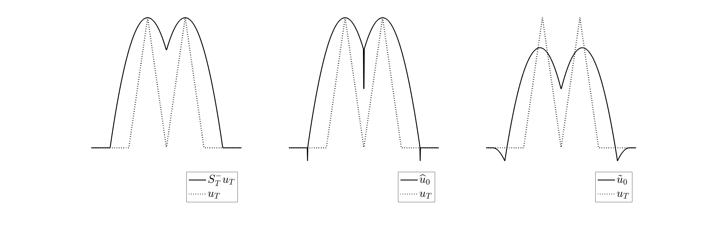
Figure 1. Different inverse designs for an unreachable target. At the left we see the inverse design obtained as the backward viscosity solution to (1) with terminal condition $u_{T}$. In the center we have the initial condition after several iterations of the approximate gradient descent algorithm described in Remark 2. At the right, we see the function $S_{T}^{-}(S_{T}^{+}\widehat{u})$, which is a regularized version of the (approximately) optimal inverse design depicted in the center.

1.2. Previous related results on inverse design for Hamilton-Jacobi equations

One of the main motivations of the present work arises in the context of inverse-time design problems associated to (1), in which, for a given (possibly noisy) observation $u_{T}$ of the solution at some time $T>0$, one aims at reconstructing the corresponding initial condition. In the recent works [23, 30], it is shown that this inverse problem is highly ill-posed. In one hand, the given observation $u_{T}$ might not be reachable, meaning that there exists no initial condition for which the viscosity solution coincides with $u_{T}$ at time $T$. On the other hand, when an inverse design for $u_{T}$ exists, it might not be unique.

In [30], we treated the case of $x$-independent Hamiltonians $H(x,p)=H(p)$ satisfying the following properties

(12) $$H\in C^{2}(\mathbb{R}^{N}),\qquad H_{pp}(p)>0\quad\forall p\in\mathbb{R}^{N}\quad\text{and}\quad\lim_{|p|\to\infty}\dfrac{H(p)}{|p|}=+\infty.$$

We showed that, in this case, existence and uniqueness of inverse designs are intimately related to the regularity of the target $u_{T}$. More precisely, the existence of at least an inverse design depends on the semiconcavity properties of $u_{T}$, whereas the uniqueness is related to its differentiability.

In the case when there exists no initial condition $u_{0}\in\operatorname{Lip}(\mathbb{R}^{N})$ such that $S_{T}^{+}u_{0}=u_{T}$, the question that arises naturally is that of constructing an initial condition $\widehat{u}_{0}\in\operatorname{Lip}(\mathbb{R}^{N})$ such that $S_{T}^{+}\widehat{u}_{0}$ is “as close as possible” to $u_{T}$. Of course, one can consider different criteria to measure the closeness of $S_{T}^{+}\widehat{u}_{0}$ to the target $u_{T}$. In this work we consider the $L^{2}$-distance, but other choices can be considered. We refer to [33, 34] for similar results for the one-dimensional Burgers equation with convex flux, and to [6] for a one-dimensional conservation law with a discontinuous space-dependent flux.

For the case of $x$-independent Hamiltonians satisfying (12), we studied in [30] the reachable function $u_{T}^{\ast}$ obtained after a backward-forward resolution of (1) with terminal condition $u_{T}$. This method gives rise to the smallest element in $\mathcal{R}_{T}$ which is bounded from below by $u_{T}$, the so-called semiconcave envelope of $u_{T}$. Hence, the inverse design $u_{0}=S_{T}^{-}u_{T}$, is optimal if one wants to approximate $u_{T}$ with functions lying above $u_{T}$. Moreover, for the case of $x$-independent quadratic Hamiltonians of the form

$$H(p)=\dfrac{\langle Ax,\,x\rangle}{2}\qquad\text{with $A$ being any positive definite matrix,}$$

we proved in [30] that the function $u^{\ast}_{T}:=S_{T}^{+}(S_{T}^{-}u_{T})$, obtained after a backward-forward resolution of (1) in the time interval $[0,T]$, actually coincides with the unique viscosity solution to the degenerate elliptic obstacle problem

$$\min\left\{\varphi-u_{T},\ -\lambda_{N}\left[D^{2}\varphi-\dfrac{A^{-1}}{T}\right]\right\}=0,$$

where, for an $N\times N$ symmetric matrix $X$, we denote by $\lambda_{N}[X]$ the greatest eigenvalue of $X$.

In the present work, for a given target $u_{T}\in\operatorname{Lip}(\mathbb{R}^{N})$ with compact support and a $p$-convex Hamiltonian $H(x,p)$ which may depend also on the space-variable $x$, instead of approximating $u_{T}$ by the backward-forward method, we consider the problem of finding a reachable function $u_{T}^{\ast}\in\mathcal{R}_{T}$ that minimizes the $L^{2}$-distance to $u_{T}$. In Figure 2, we can see an illustration of the semiconcave envelope of an unreachable target function $u_{T}$, compared with the $L^{2}$-projection of $u_{T}$ onto $\mathcal{R}_{T}$. Observe that, since the semiconcave envelope always lies above the target, the projection obtained by the operator $S_{T}^{+}\circ S_{T}^{-}$ is different to the $L^{2}$-projection of $u_{T}$ onto $\mathcal{R}_{T}$, unless the target $u_{T}$ is reachable.

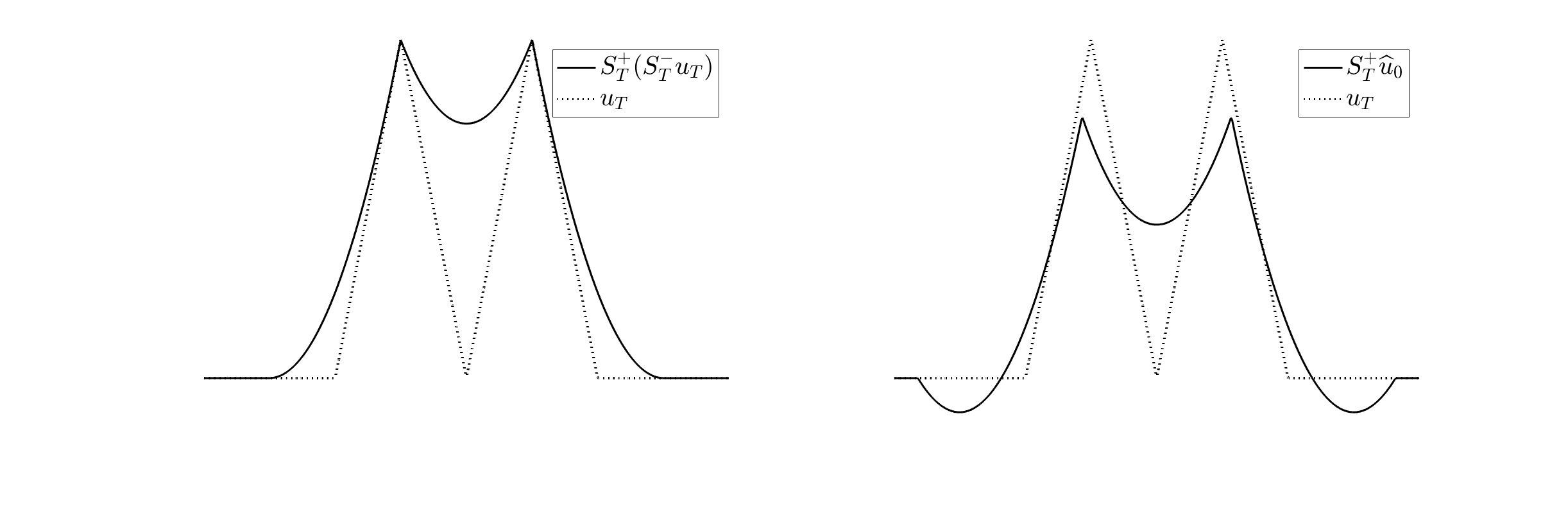
Figure 2. At the left we see the semiconcave envelope of a function $u_{T}\in\operatorname{Lip}(\mathbb{R})$, obtained by a backward-forward resolution of (1), i.e. the smallest reachable function bounded from below by $u_{T}$. At the right we see the $L^{2}$-projection of $u_{T}$ onto the reachable set $\mathcal{R}_{T}$, i.e. the reachable function which minimizes the $L^{2}$-distance to $u_{T}$.

The rest of the paper is structured as follows. In Section 2, we present and prove the main results concerning the differentiability of the forward viscosity operator $S_{T}^{+}$ with respect to the initial condition. The proof of Theorem 1 is postponed to the subsection 2.3. In subsection 2.2, we compute the gradient of the functional $\mathcal{J}_{T}$ and derive a first-order optimality condition for the optimal control problem (8). In section 3, for the one-dimensional case, and for quadratic Hamiltonians in any space dimension, we identify the directional Gâteaux derivatives obtained in Section 2, with duality solutions to the transport equation (4). The main result of this section is stated in subsection 3.1, and its proof is postponed to subsection 3.5. In subsection 3.2, we represent the gradient of the functional $\mathcal{J}_{T}$, defined in (8), by means of the unique backward solution at time $t=0$ to the dual equation to (4), which is the backward conservative equation (10). In subsection 3.3, we recall the main definitions and properties of duality solutions, as presented in [16]. In subsection 3.4, we give a proof of a semiconcavity estimate, necessary in the proof of Theorem 3. Finally, in Section 4 we give the proof of the existence of minimizers for the optimal control problem 8. In addition, for the case when the Hamiltonian is $x-$independent and quadratic, we prove that the $L^{2}$-projection of any $u_{T}\in\operatorname{Lip}(\mathbb{R}^{N})$ onto the space of reachable targets $\mathcal{R}_{T}$ is unique.

2. Differentiability with respect to the initial condition

The goal in this section is to prove that the forward viscosity operator $S_{T}^{+}$ defined in (3) is differentiable with respect to the $L^{1}_{loc}$-convergence. Then, we use this differentiability result to compute the gradient of the functional $\mathcal{J}_{T}$ defined in (8), which allows us to derive a first-order optimality condition for the optimization problem (8).

It is well known (see for instance [31, Chapter 10] or [32, Section I.10]) that, under the hypotheses (H1),(H2), (H3) and (H4), for any initial condition $u_{0}\in\operatorname{Lip}(\mathbb{R}^{N})$, the unique viscosity solution to (1) can be given by the value function of an associated problem in the calculus of variations as follows:

(13) $$u(t,x)=\inf_{\begin{subarray}{c}\xi\in W^{1,1}((0,t);\mathbb{R}^{N})\\ \xi(t)=x\end{subarray}}\left\{\int_{0}^{t}H^{\ast}(\xi(s),\,\dot{\xi}(s))ds+u_{0}(\xi(0))\right\},\qquad\forall(t,x)\in[0,T]\times\mathbb{R}^{N}$$

where $H^{\ast}:\mathbb{R}^{N}\times\mathbb{R}^{N}\to\mathbb{R}$ denotes the Legendre-Fenchel transform of $H(x,\cdot)$, i.e.

$$H^{\ast}(x,q)=\max_{p\in\mathbb{R}^{N}}\left\{p\cdot q-H(x,p)\right\}\qquad\forall x,q\in\mathbb{R}^{N}.$$

In view of the representation formula (13), for any $t\in(0,T]$, the forward viscosity operator $S_{t}^{+}$ introduced in (3) can be given by the expression

(14) $$S_{t}^{+}u_{0}(x):=\inf_{\begin{subarray}{c}\xi\in W^{1,1}((0,t);\mathbb{R}^{N})\\ \xi(t)=x\end{subarray}}\left\{\int_{0}^{t}H^{\ast}(\xi(s),\,\dot{\xi}(s))ds+u_{0}(\xi(0))\right\},\qquad\forall x\in\mathbb{R}^{N}.$$

One can readily prove that the operator $S_{t}^{+}$ satisfies the semigroup property

$$(S_{t_{1}}^{+}\circ S_{t_{2}}^{+})u_{0}=S_{t_{1}+t_{2}}^{+}u_{0},\qquad\forall t_{1},\,t_{2}>0.$$

2.1. Differentiability of the forward viscosity semigroup

The main result of this section is the following theorem, which states that the operator $S_{t}^{+}$ is Gâteaux differentiable at any $u_{0}\in\operatorname{Lip}(\mathbb{R}^{N})$, in any direction $w\in\operatorname{Lip}(\mathbb{R}^{N})$. The proof of this theorem is postponed to subsection 2.3.

Theorem 1.

Let $T>0$, $u_{0}\in\operatorname{Lip}(\mathbb{R}^{N})$, and let $H$ be a Hamiltonian satisfying (H1),(H2), (H3) and (H4). Let $S_{t}^{+}$ be the forward viscosity operator defined in (14). Then, for any $w\in\operatorname{Lip}(\mathbb{R}^{N})$ and $t\in(0,T]$ we have

$$\dfrac{S_{t}^{+}(u_{0}+\delta w)(\cdot)-S_{t}^{+}u_{0}(\cdot)}{\delta}\longrightarrow\partial_{w}S_{t}^{+}u_{0}(\cdot)\quad\text{as}\quad\delta\to 0^{+},\quad\text{in}\quad L^{1}_{loc}(\mathbb{R}^{N}),$$

where $\partial_{w}S_{t}^{+}u_{0}(\cdot)\in L^{\infty}_{loc}(\mathbb{R}^{N})$ is defined almost everywhere in $\mathbb{R}^{N}$ in the following way:

At any point $x\in\mathbb{R}^{N}$ where $S_{t}^{+}u_{0}(\cdot)$ is differentiable, we have

(15) $$\partial_{w}S_{t}^{+}u_{0}(x)=w(\xi_{t,x}(0)),$$

with $(\xi_{t,x}(\cdot),p_{t,x}(\cdot))\in C^{1}([0,t];\mathbb{R}^{N})$ being the unique solution to the backward system of ODEs

(16) $$\left\{\begin{array}[]{ll}\dot{\xi}_{t,x}(s)=H_{p}(\xi_{t,x}(s),p_{t,x}(s))&s\in(0,t)\\ \vspace{2pt}\cr\dot{p}_{t,x}(s)=-H_{x}(\xi_{t,x}(s),p_{t,x}(s))&s\in(0,t)\\ \vspace{2pt}\cr\xi_{t,x}(t)=x\quad p_{t,x}(t)=\nabla S_{t}^{+}u_{0}(x).\end{array}\right.$$

(Note that, since $S_{t}^{+}u_{0}(\cdot)\in\operatorname{Lip}(\mathbb{R}^{N})$, by means of Rademacher’s Theorem we have that $S_{t}^{+}u_{0}(\cdot)$ is differentiable almost everywhere in $\mathbb{R}^{N}$. Hence, the expression (15) uniquely determines $\partial_{w}S_{t}^{+}u_{0}(\cdot)$ as an element of $L^{\infty}_{loc}(\mathbb{R}^{N})$).

The function $\partial_{w}S_{t}^{+}u_{0}(\cdot)\in L^{\infty}_{loc}(\mathbb{R}^{N})$ defined a.e. as in (15) can be interpreted as the Gâteaux derivative of the operator $S_{t}^{+}$ at $u_{0}$ in the direction $w$. Now, for any $u_{0}\in\operatorname{Lip}(\mathbb{R}^{N})$ and $t\in(0,T]$ fixed, let us define the function $\Phi_{u_{0}}^{t}(\cdot)\in L_{loc}^{\infty}(\mathbb{R}^{N};\mathbb{R}^{N})$ as

(17) $$\Phi_{u_{0}}^{t}(x):=\xi_{t,x}(0),\qquad\text{for a.e.}\ x\in\mathbb{R}^{N},$$

where $\xi_{t,x}(0)$ is the unique solution to (16). Then, the operator

$$\begin{array}[]{ccclc}DS_{t}^{+}(u_{0}):&\operatorname{Lip}(\mathbb{R}^{N})&\longrightarrow&L^{\infty}_{loc}(\mathbb{R}^{N})\\ \vspace{2pt}\cr&w(\cdot)&\longmapsto&\partial_{w}S_{t}^{+}u_{0}(\cdot):=w(\Phi_{u_{0}}^{t}(\cdot))&\text{a.e. in}\ \mathbb{R}^{N}\end{array}$$

is linear and continuous in its domain, and can be seen as the gradient of the operator $S_{t}^{+}$ at $u_{0}$. This proves that for any $t\in(0,T]$, the operator $S_{t}^{+}$ defined in (14) is differentiable with respect to the $L^{1}_{loc}$-convergence.

Remark 3 (Lipschitz continuity).

Note moreover that, for any $u_{0}\in\operatorname{Lip}(\mathbb{R}^{N})$, the norm of the linear operator $DS_{t}^{+}(u_{0})$ above defined, restricted to $\operatorname{Lip}(\mathbb{R}^{N})\cap L^{\infty}(\mathbb{R}^{N})$, is equal to $1$. This implies that, for any $t\in(0,T]$, the forward viscosity operator $S_{t}^{+}$, restricted to $\operatorname{Lip}(\mathbb{R}^{N})\cap L^{\infty}(\mathbb{R}^{N})$, is Lipschitz with constant $1$, i.e.

$$\|S_{t}^{+}u_{0}-S_{t}^{+}u_{1}\|_{L^{\infty}(\mathbb{R}^{N})}\leq\|u_{0}-u_{1}\|_{L^{\infty}(\mathbb{R}^{N})}\quad\text{for all}\quad u_{0},u_{1}\in\operatorname{Lip}(\mathbb{R}^{N})\cap L^{\infty}(\mathbb{R}^{N}).$$

This inequality is also proved in (28) as part of the proof of Theorem 1.

2.2. First-order optimality condition for inverse designs

In this subsection, for a given time horizon $T>0$ and a target function $u_{T}\in\operatorname{Lip}_{0}(\mathbb{R}^{N})$, we consider the optimization problem (8), presented in the introduction, of constructing an initial condition for which the corresponding viscosity solution to (1) at time $T$ minimizes the $L^{2}$-distance to $u_{T}$. Using the forward viscosity operator $S_{T}^{+}$ introduced in (3), and given explicitly by the expression (14), the problem can be formulated as

(18) $$\underset{u_{0}\in\operatorname{Lip}_{0}(\mathbb{R}^{N})}{\text{minimize}}\ \mathcal{J}_{T}(u_{0}):=\|S_{T}^{+}u_{0}(\cdot)-u_{T}(\cdot)\|_{L^{2}(\mathbb{R}^{N})}^{2}.$$

Remark 4 (Assumptions on the Hamiltonian).

We address the optimization problem (18) under the assumption that the Hamiltonian $H$ satisfies the hypotheses (H1), (H3), (H4), and (H2) with $C_{0}=0$. This choice guarantees that the operator $S_{T}^{+}$ defined in (14) satisfies

(19) $$S_{T}^{+}u_{0}\in\operatorname{Lip}_{0}(\mathbb{R}^{N})\qquad\forall u_{0}\in\operatorname{Lip}_{0}(\mathbb{R}^{N}).$$

Indeed, it is easy to check that condition (H2) with $C_{0}=0$ implies the same property on the Legendre-Fenchel transform $H^{\ast}$, i.e.

$$H^{\ast}(x,q)\geq 0\quad\forall x,q\in\mathbb{R}^{N}\quad\text{and}\quad H^{\ast}(x,0)=0\quad\forall x\in\mathbb{R}^{N}.$$

This property implies in particular that $S_{T}^{+}0=0$, and then, by using the compactness estimates from [5, Corollary 1] (see also [4]), we deduce that, if $u_{0}\in\operatorname{Lip}_{0}(\mathbb{R}^{N})$, there exists a constant $l>0$ such that $\operatorname{supp}(S_{T}^{+}u_{0})\subset[-l,l]^{N}$. Finally, since $\operatorname{Lip}_{0}(\mathbb{R}^{N})\subset L^{2}(\mathbb{R}^{N})$, property (19) follows. Having property (19) in hand, we deduce that the set of admissible initial conditions for the optimization problem (18), i.e. $u_{0}\in\operatorname{Lip}(\mathbb{R}^{N})$ satisfying $\mathcal{J}_{T}(u_{0})<\infty$, is nonempty.

Remark 5 (Existence of minimizers).

Note that, due to the lack of backward uniqueness of the Hamilton-Jacobi equation (1), the functional $\mathcal{J}_{T}(\cdot)$ is not expected to be coercive. Indeed, in view of the results in [23, 30], the preimage by $S_{T}^{+}$ of any reachable function $\varphi_{T}\in\mathcal{R}_{T}$ consists of a convex cone in $\operatorname{Lip}(\mathbb{R}^{N})$, which might be unbounded in $L^{2}(\mathbb{R}^{N})$. The existence of a minimizer for the problem (18) can however be justified by using the backward viscosity operator $S_{T}^{-}$ defined in (62). We shall prove, in Theorem 8 in Section 4, the existence of at least one minimizer for the optimization problem (18).

In the following theorem, we derive a first-order optimality condition for the problem (18). This is done by using the differentiability result from Theorem 1, which allows one to compute the directional derivatives of the functional

$$\begin{array}[]{cccc}\mathcal{J}_{T}:&\operatorname{Lip}_{0}(\mathbb{R}^{N})&\longrightarrow&\mathbb{R}\\ \vspace{2pt}\cr&u_{0}&\longmapsto&\|S_{T}^{+}u_{0}(\cdot)-u_{T}(\cdot)\|_{L^{2}(\mathbb{R}^{N})}^{2}.\end{array}$$

Theorem 2.

Let $T>0$ and let $H$ be a Hamiltonian satisfying (H1), (H3), (H4), and (H2) with $C_{0}=0$. Let $S_{T}^{+}$ be the forward viscosity operator defined in (14), and let $u_{T}\in\operatorname{Lip}_{0}(\mathbb{R}^{N})$ be a given function with compact support. Then, any $u_{0}\in\operatorname{Lip}_{0}(\mathbb{R}^{N})$ solution to the optimization problem (18) satisfies

(20) $$\int_{\mathbb{R}^{N}}(S_{T}^{+}u_{0}(x)-u_{T}(x))\,w(\Phi_{u_{0}}^{T}(x))dx=0\quad\forall w\in\operatorname{Lip}(\mathbb{R}^{N}).$$

This condition can also be expressed, in terms of the gradient of the functional $\mathcal{J}_{T}$, as

$$D\mathcal{J}_{T}(u_{0})=0,$$

where $D\mathcal{J}_{T}$ is the continuous linear functional

(21) $$\begin{array}[]{ccccl}D\mathcal{J}_{T}(u_{0}):&\operatorname{Lip}(\mathbb{R}^{N})&\rightarrow&\mathbb{R}\\ \vspace{2pt}\cr&w(\cdot)&\mapsto&\partial_{w}\mathcal{J}_{T}(u_{0})&:=2\displaystyle\int_{\mathbb{R}^{N}}(S_{T}^{+}u_{0}(x)-u_{T}(x))\,w(\Phi_{u_{0}}^{T}(x))dx\end{array}$$

with $\Phi_{u_{0}}^{T}:\mathbb{R}^{N}\to\mathbb{R}^{N}$ being the map defined a.e. as in (17). Note that, by the density of Lipschitz functions in $C_{c}^{0}(\mathbb{R}^{N})$, we can extend the functional $D\mathcal{J}_{T}(u_{0})$ to $C_{c}^{0}(\mathbb{R}^{N})$, and we then deduce that $D\mathcal{J}_{T}(u_{0})$ defines a Radon measure in $\mathbb{R}^{N}$.

Proof.

Using the conclusions of Theorem 1, and the fact that $u_{0},u_{T}\in\operatorname{Lip}_{0}(\mathbb{R}^{N})$ are compactly supported, we can compute

$$\lim_{\delta\to 0^{+}}\dfrac{\mathcal{J}_{T}(u_{0}+\delta w)-\mathcal{J}_{T}(u_{0})}{\delta} = \lim_{\delta\to 0^{+}}2\displaystyle\int_{\mathbb{R}^{N}}(S_{T}^{+}u_{0}(x)-u_{T}(x))\dfrac{S_{T}^{+}(u_{0}+\delta w)(x)-S_{T}^{+}u_{0}(x)}{\delta}dx$$

$$= 2\displaystyle\int_{\mathbb{R}^{N}}(S_{T}^{+}u_{0}(x)-u_{T}(x))\partial_{w}S_{T}^{+}u_{0}(x)dx,$$

where $\partial_{w}S_{T}^{+}u_{0}\in L^{\infty}_{loc}(\mathbb{R}^{N})$ is given by (15). Hence, using the map $\Phi_{u_{0}}^{T}$ defined a.e. in (17), we can write the directional derivative of $\mathcal{J}_{T}$ at $u_{0}$ in the direction $w$ as

$$\partial_{w}\mathcal{J}_{T}(u_{0})=2\int_{\mathbb{R}^{N}}(S_{T}^{+}u_{0}(x)-u_{T}(x))\,w(\Phi_{u_{0}}^{T}(x))dx.$$

This gives the first-order optimality condition (20).

Finally, note that the functional $D\mathcal{J}_{T}$ defined in (21) is clearly linear and continuous with respect to the sup-norm in $C_{c}^{0}(\mathbb{R}^{N})$. Then, by the density of $\operatorname{Lip}(\mathbb{R}^{N})$ in the space of continuous functions with compact support, we can identify $D\mathcal{J}_{T}(u_{0})$ with a Radon measure in $\mathbb{R}^{N}$. ∎

2.3. Proof of Theorem 1

Let us give the proof of Theorem 1. As a first step we provide, in Proposition 1, an explicit expression for the limit

$$\lim_{\delta\to 0^{+}}\dfrac{S_{t}^{+}(u_{0}+\delta w)(x)-S_{t}^{+}u_{0}(x)}{\delta}.$$

at the points $x\in\mathbb{R}^{N}$ where $S_{t}^{+}u_{0}$ is differentiable. As it is well-known, the viscosity solution to (1) is Lipschitz continuous, and then, by Rademacher’s Theorem, $S_{t}^{+}u_{0}$ is differentiable for a.e. $x\in\mathbb{R}^{N}$. Therefore, Proposition 1 is sufficient to explicitly identify a unique candidate in $L^{\infty}_{loc}(\mathbb{R}^{N})$ for the directional Gâteaux derivative $\partial_{w}S_{t}^{+}u_{0}(\cdot)$.

Proposition 1.

Let $T>0$, $u_{0}\in\operatorname{Lip}(\mathbb{R}^{N})$ and $H$ be a Hamiltonian satisfying (H1),(H2), (H3) and (H4). For any $t\in(0,T]$, let $S_{t}^{+}$ be the forward viscosity operator defined in (14). For any $x\in\mathbb{R}^{N}$ such that $S_{t}^{+}u_{0}(\cdot)$ is differentiable at $x$, let $\xi_{t,x}\in C^{1}([0,t];\mathbb{R}^{N})$, together with $p_{t,x}\in C^{1}([0,t];\mathbb{R}^{N})$, be the unique solution to the terminal value problem

(22) $$\left\{\begin{array}[]{ll}\dot{\xi}_{t,x}(s)=H_{p}(\xi_{t,x}(s),p_{t,x}(s))&s\in(0,t)\\ \vspace{2pt}\cr\dot{p}_{t,x}(s)=-H_{x}(\xi_{t,x}(s),p_{t,x}(s))&s\in(0,t)\\ \vspace{2pt}\cr\xi_{t,x}(t)=x\quad p_{t,x}(t)=\nabla S_{t}^{+}u_{0}(x).\end{array}\right.$$

Then, for any $w\in\operatorname{Lip}(\mathbb{R}^{N})$, we have

$$\lim_{\delta\to 0^{+}}\dfrac{S_{t}^{+}(u_{0}+\delta w)(x)-S_{t}^{+}u_{0}(x)}{\delta}=w(\xi_{t,x}(0)).$$

Remark 6.

This result proves that, for any $x\in\mathbb{R}^{N}$ fixed, the map

$$u_{0}(\cdot)\in\operatorname{Lip}(\mathbb{R}^{N})\longmapsto S_{t}^{+}u_{0}(x)\in\mathbb{R}$$

is differentiable at any $u_{0}\in\operatorname{Lip}(\mathbb{R}^{N})$ where $S_{t}^{+}u_{0}(\cdot)$ is differentiable. However, it does not directly prove the differentiability of the operator $S_{t}^{+}$. Indeed, Proposition 1 proves that the limit

$$\dfrac{S_{t}^{+}(u_{0}+\delta w)(\cdot)-S_{t}^{+}u_{0}(\cdot)}{\delta}\to\partial_{w}S_{t}^{+}u_{0}(\cdot)\qquad\text{as}\ \delta\to 0^{+}.$$

holds in the sense almost everywhere in $\mathbb{R}^{N}$, and represents the first step of the proof of Theorem 1. The second step will consist in justifying that the convergence actually holds in $L^{1}_{loc}(\mathbb{R}^{N})$.

In the proof of Proposition 1, we use the following well-known result concerning the minimizers of the right-hand-side of (14) at the points where $S_{t}^{+}u_{0}(\cdot)$ is differentiable.

Lemma 1.

Let $T>0$, $u_{0}\in\operatorname{Lip}(\mathbb{R}^{N})$ and $H$ be a Hamiltonian satisfying (H1),(H2), (H3) and (H4). For any $(t,x)\in(0,T]\times\mathbb{R}^{N}$ fixed, let $\xi_{t,x}(\cdot)$ be any minimizing trajectory for the right-hand side of (14), and let $p_{t,x}(\cdot)$ be its associated dual arc. Then, the following statements hold true:

1. For all $s\in(0,t)$, the function $S_{s}^{+}u_{0}(\cdot)$ is differentiable at $\xi_{t,x}(s)$, and

   $$\nabla S_{s}^{+}u_{0}(\xi_{t,x}(s))=p_{t,x}(s).$$

2. If $S_{t}^{+}u_{0}(\cdot)$ is differentiable at $x$, then the minimizer $\xi_{t,x}$ of the right-hand-side in (14) is unique and is given by the unique solution to (22).

Proof.

The result is well-known and is a direct consequence of the results in Chapter 6 in [22]. Let us give a brief sketch of the proof for the reader’s convenience. The first statement follows directly from [22, Theorem 6.4.8]. For the second statement, sing [22, Theorem 6.4.10], the differentiability of $S_{t}^{+}u_{0}(\cdot)$ at $x$ implies that $(t,x)$ is a regular point in the sense of [22, Definition 6.3.4], i.e. the minimizer $\xi_{x}$ of the right-hand-side in (14) is unique. Then the proof can be concluded by using Theorems 6.3.3 and 6.4.8 in [22]. ∎

We can now proceed to the proof of Proposition 1.

Proof of Proposition 1.

Let $(t,x)\in(0,T]\times\mathbb{R}^{N}$ be such that $S_{t}^{+}u_{0}(\cdot)$ is differentiable at $x$, and let $\xi_{t,x}(\cdot)\in C^{1}([0,t];\mathbb{R}^{N})$ be the solution to (22). We first note that, in view of (14) and Lemma 1, we have

$$S_{t}^{+}u_{0}(x)=\int_{0}^{t}H^{\ast}(\xi_{t,x}(s),\dot{\xi}_{t,x}(s))ds+u_{0}(\xi_{t,x}(0))$$

and

$$S_{t}^{+}(u_{0}+\delta w)(x)\leq\int_{0}^{t}H^{\ast}(\xi_{t,x}(s),\dot{\xi}_{t,x}(s))ds+u_{0}(\xi_{t,x}(0))+\delta w(\xi_{t,x}(0)),$$

which combined together imply

$$\dfrac{S_{t}^{+}(u_{0}+\delta w)(x)-S_{t}^{+}u_{0}(x)}{\delta}\leq w(\xi_{t,x}(0))\qquad\forall\delta>0.$$

Hence, we have

(23) $$\limsup_{\delta\to 0^{+}}\dfrac{S_{t}^{+}(u_{0}+\delta w)(x)-S_{t}^{+}u_{0}(x)}{\delta}\leq w(\xi_{t,x}(0)).$$

Let us now prove that

(24) $$\liminf_{\delta\to 0^{+}}\dfrac{S_{t}^{+}(u_{0}+\delta w)(x)-S_{t}^{+}u_{0}(x)}{\delta}\geq w(\xi_{t,x}(0)).$$

We argue by contradiction. Let us suppose that there exists $\alpha>0$ and a sequence $\{\delta_{n}\}_{n\in\mathbb{N}}$ such that $\delta_{n}\in(0,1)$, $\delta_{n}\to 0$ and

(25) $$\dfrac{S_{t}^{+}(u_{0}+\delta_{n}w)(x)-S_{t}^{+}u_{0}(x)}{\delta_{n}}\leq w(\xi_{t,x}(0))-\alpha\qquad\forall n\in\mathbb{N}.$$

For each $n\in\mathbb{N}$, let $\xi_{n}\in C^{1}(0,t;\mathbb{R}^{N})$ be such that

$$S_{t}^{+}(u_{0}+\delta_{n}w)(x)=\int_{0}^{t}H^{\ast}(\xi_{n}(s),\dot{\xi}_{n}(s))ds+u_{0}(\xi_{n}(0))+\delta_{n}w(\xi_{n}(0)).$$

Using (14), we deduce

$$S_{t}^{+}u_{0}(x)+\delta_{n}w(\xi_{n}(0)) = \int_{0}^{t}H^{\ast}(\xi_{t,x}(s),\dot{\xi}_{t,x}(s))ds+u_{0}(\xi_{t,x}(0))+\delta_{n}w(\xi_{n}(0))$$

$$\leq \int_{0}^{t}H^{\ast}(\xi_{n}(s),\dot{\xi}_{n}(s))ds+u_{0}(\xi_{n}(0))+\delta_{n}w(\xi_{n}(0))$$

$$= S_{t}^{+}(u_{0}+\delta_{n}w)(x),$$

which combined with (25) implies

(26) $$w(\xi_{n}(0))\leq\dfrac{S_{t}^{+}(u_{0}+\delta_{n}w)(x)-S_{t}^{+}u_{0}(x)}{\delta_{n}}\leq w(\xi_{t,x}(0))-\alpha\qquad\forall n\in\mathbb{N}.$$

Using the fact that the function $u_{0}+\delta_{n}w$ is globally Lipschitz with a Lipschitz constant independent of $n$, we deduce from Lemma 1, and using the hypothesis (H3), that there exists a constant $C_{T}>0$ such that the viscosity solution $u_{n}\in\operatorname{Lip}([0,T]\times\mathbb{R}^{N})$ to (1) with initial condition $u_{0}+\delta_{n}w$ is Lipschitz continuous with Lipschitz constant $C_{T}$ independent of $n\in\mathbb{N}$. This implies in particular that the dual arc $p_{n}(\cdot)$ associated to each optimal trajectory $\xi_{n}(\cdot)$ satisfies

$$|p_{n}(s)|\leq C_{T}\qquad\forall s\in[0,t].$$

We then deduce, using (H4), that there exists another constant $C_{T}^{\prime}>0$, also independent of $n$, such that

$$|\dot{\xi}_{n}(s)|\leq C_{T}^{\prime}\qquad\forall s\in[0,t]\quad\forall n\in\mathbb{N}.$$

Hence, by Arzéla-Ascoli Theorem, there exists $\xi_{\infty}(\cdot)\in W^{1,1}(0,T;\mathbb{R}^{N})$ such that $\xi_{n}(\cdot)\to\xi_{\infty}(\cdot)$ uniformly in $(0,t)$.

Now, in view of (26), we deduce that $\xi_{\infty}(\cdot)\neq\xi_{t,x}(\cdot)$, which combined with the fact that, by means of Lemma 1 (ii), $\xi_{t,x}(\cdot)$ is the unique minimizer for the right-hand-side of (14), implies that there exists $\beta>0$ such that

$$\int_{0}^{t}H^{\ast}(\xi_{\infty}(s),\dot{\xi}_{\infty}(s))ds+u_{0}(\xi_{\infty}(0))=\int_{0}^{t}H^{\ast}(\xi_{t,x}(s),\dot{\xi}_{t,x}(s))ds+u_{0}(\xi_{t,x}(0))+\beta.$$

On the other hand, since $H^{\ast}(x,q)$ is continuous with respect to both variables and convex in $q$, we deduce that the right-hand-side of (14) is weakly lower semicontinuous, and then

$$\liminf_{n\to\infty}\int_{0}^{t}H^{\ast}(\xi_{n}(s),\dot{\xi}_{n}(s))ds+u_{0}(\xi_{n}(0)) \geq \int_{0}^{t}H^{\ast}(\xi_{\infty}(s),\dot{\xi}_{\infty}(s))ds+u_{0}(\xi_{\infty}(0))$$

$$= \int_{0}^{t}H^{\ast}(\xi_{t,x}(s),\dot{\xi}_{t,x}(s))ds+u_{0}(\xi_{t,x}(0))+\beta,$$

which implies that we can extract another subsequence $\delta_{n}\to 0$ such that

$$\int_{0}^{t}H^{\ast}(\xi_{n}(s),\dot{\xi}_{n}(s))ds+u_{0}(\xi_{n}(0))\geq\int_{0}^{t}H^{\ast}(\xi_{t,x}(s),\dot{\xi}_{t,x}(s))ds+u_{0}(\xi_{t,x}(0))+\dfrac{\beta}{2}\qquad\forall n\geq 1.$$

Finally, using the optimality of $\xi_{n}$ for each $n$, we have in addition that

$$\displaystyle\int_{0}^{t}H^{\ast}(\xi_{t,x}(s),\dot{\xi}_{t,x}(s))ds+u_{0}(\xi_{t,x}(0))+\delta_{n}w(\xi_{t,x}(0)) \geq \displaystyle\int_{0}^{t}H^{\ast}(\xi_{n}(s),\dot{\xi}_{n}(s))ds+u_{0}(\xi_{n}(0))$$

$$+\delta_{n}w(\xi_{n}(0))$$

for all $n\geq 1$, and adding the last two inequalities we obtain

$$\delta_{n}\left(w(\xi_{t,x}(0))-w(\xi_{n}(0))\right)\geq\dfrac{\beta}{2}>0,$$

which leads to a contradiction since $\delta_{n}\to 0$. The inequality (24) then follows, and together with (23), implies the conclusion of the theorem. ∎

Let us finish the section with the proof of Theorem 1.

Proof of Theorem 1.

In one hand, since $S_{t}^{+}u_{0}(\cdot)$ is Lipschitz continuous, and then differentiable almost everywhere in $\mathbb{R}^{N}$, by means of Proposition 1 we have

(27) $$\dfrac{S_{t}^{+}(u_{0}+\delta w)(x)-S_{t}^{+}u_{0}(x)}{\delta}\to\partial_{w}S_{t}^{+}u_{0}(x)\quad\text{for a.e. }\ x\in\mathbb{R}^{N}.$$

Now, let $K\subset\subset\mathbb{R}^{N}$ be any compact set. We claim that there exists another compact set $K^{\prime}\subset\subset\mathbb{R}^{N}$ such that, for any $\delta>0$, it holds that

(28) $$\left|\dfrac{S_{t}^{+}(u_{0}+\delta w)(x)-S_{t}^{+}u_{0}(x)}{\delta}\right|\leq\|w\|_{L^{\infty}(K^{\prime})}\qquad\forall x\in\mathbb{R}^{N}.$$

Indeed, by the definition of $S_{t}^{+}$ in (14), for any $x\in K$ there exists $\xi_{1}\in C^{1}(0,t;\mathbb{R}^{N})$ such that

$$S_{t}^{+}u_{0}(x)=\int_{0}^{t}H^{\ast}(\xi_{1}(s),\dot{\xi}_{1}(s))ds+u_{0}(\xi_{1}(0)),$$

which then implies that

$$S_{t}^{+}(u_{0}+\delta w)(x)-S_{t}^{+}u_{0}(x) \leq \int_{0}^{t}H^{\ast}(\xi_{1}(s),\dot{\xi}_{1}(s))ds+u_{0}(\xi_{1}(0))+\delta w(\xi_{1}(0))$$

$$-\int_{0}^{t}H^{\ast}(\xi_{1}(s),\dot{\xi}_{1}(s))ds-u_{0}(\xi_{1}(0))$$

$$= \delta w(\xi_{1}(0)).$$

Moreover, using the hypotheses (H3) and (H4), we deduce that the trajectory $\xi_{1}(\cdot)$ is contained in a compact set $K^{\prime}\subset\subset\mathbb{R}^{N}$ independent of $x\in K$, which in turn implies, combined with (2.3), that

$$S_{t}^{+}(u_{0}+\delta w)(x)-S_{t}^{+}u_{0}(x)\leq\delta\|w\|_{L^{\infty}(K^{\prime})}.$$

Using a similar argument, with an arc $\xi_{2}\in C^{1}(0,t;\mathbb{R}^{N})$ minimizing the right-hand-side of (14) with $u_{0}+\delta w$ instead of $u_{0}$ we obtain

$$S_{t}^{+}(u_{0}+\delta w)(x)-S_{t}^{+}u_{0}(x)\geq\delta w(\xi_{2}(0))\geq-\delta\|w\|_{L^{\infty}(K^{\prime})},$$

and then (28) follows.

Now, in view of (27) and (28), we can use Lebesgue’s dominated convergence Theorem to deduce

$$\lim_{\delta\to 0^{+}}\int_{K}\left|\dfrac{S_{t}^{+}(u_{0}+\delta w)(x)-S_{t}^{+}u_{0}(x)}{\delta}-\partial_{w}S_{t}^{+}u_{0}(x)\right|dx=0,\quad\text{for all compact set $K\subset\subset\mathbb{R}^{N}$,}$$

which implies that

$$\dfrac{S_{t}^{+}(u_{0}+\delta w)-S_{t}^{+}u_{0}}{\delta}\longrightarrow\partial_{w}S_{t}^{+}u_{0},\qquad\text{as}\quad\delta\to 0^{+}\quad\text{in}\ L^{1}_{loc}(\mathbb{R}^{N}).$$

∎

3. Gâteaux derivatives and linear transport equations

The goal in this section is to prove that, for any $u_{0},w\in\operatorname{Lip}(\mathbb{R}^{N})$, the directional Gateaux derivative $\partial_{w}S_{T}^{+}u_{0}$, that we proved to exist in Theorem 1, is actually the unique duality solution to the following linear transport equation:

(30) $$\left\{\begin{array}[]{ll}\partial_{t}v+a(t,x)\cdot\nabla_{x}v=0&(t,x)\in(0,T)\times\mathbb{R}^{N}\\ v(0,x)=w(x)&x\in\mathbb{R}^{N},\end{array}\right.$$

where the transport coefficient $a(t,x)$ is given by

(31) $$a(t,x):=H_{p}(x,\nabla_{x}[S_{t}^{+}u_{0}(x)]).$$

The precise definition and the main properties of duality solutions for the equation (30) are given in subsection 3.3. We refer to [14, 16] for further details concerning the theory of duality solutions for transport equations with discontinuous transport coefficient satisfying a one-sided-Lipschitz condition.

As it is well-known, when $t>0$ is sufficiently large, the solution to (1) eventually looses regularity and its gradient develops jump-discontinuities. This in turn implies that the transport coefficient (31) is no longer continuous, and therefore, the equation (30) cannot be solved by the classical method of characteristics. A key-feature in our proof to establish well-posedness for (30) is the fact that the transport coefficient $a(t,x)$ defined in (31) satisfies the following one-sided Lipschitz condition (OSLC)

(32) $$\langle a(t,y)-a(t,x),\,y-x\rangle\leq\dfrac{C}{t}|y-x|^{2}\qquad\text{for a.e.}\ (t,x,y)\in(0,T)\times\mathbb{R}^{N}\times\mathbb{R}^{N},$$

where $C>0$ is a positive constant. In the work by Bouchut-James-Mancini [16], existence, uniqueness and stability is established for linear transport equations as (30) with a transport coefficient satisfying the OSLC condition. However, we are not able to directly apply the results in [16] since the function $\alpha(t)=C/t$ does not belong to $L^{1}(0,T)$. Moreover, we are only able to treat the one-dimensional case in space, and the case of quadratic Hamiltonians of the form

(33) $$H(x,p)=|p|^{2}+f(x),$$

where $f\in C^{2}(\mathbb{R}^{N})$ is bounded and globally Lipschitz. In these two cases, (32) can be deduced from the semiconcavity of the viscosity solution, whereas this is not the case for general convex Hamiltonians in dimension higher than 1.

3.1. Directional Gâteaux derivatives as duality solutions

Let us state the main result of this section, which ensures that the directional Gâteaux derivative of the forward viscosity operator $S_{T}^{+}$ at $u_{0}$ in the direction $w$ is the unique duality solution to the linear transport equation (30).

Theorem 3.

Let $T>0$, $u_{0},w\in\operatorname{Lip}(\mathbb{R}^{N})$, and let, either $N=1$ and $H$ be a Hamiltonian satisfying (H1), (H2), (H3) and (H4), or let $N>1$ and $H$ be of the form (33). Then we have

$$\dfrac{S_{t}^{+}(u_{0}+\delta w)(x)-S_{t}^{+}u_{0}(x)}{\delta}\to v(t,x)\qquad\text{in}\ C([0,T],L^{1}_{loc}(\mathbb{R}^{N}))$$

where $v(t,x)$ is the unique duality solution to the linear transport equation (30) with transport coefficient $a(t,x)$ given by (31) and initial condition $v(0,\cdot)=w(\cdot)$.

The proof of this theorem is postponed to subsection 3.5, and relies on the well-posedness of the dual equation to (30), which is the backward conservative equation

(34) $$\left\{\begin{array}[]{ll}\partial_{t}\pi+\operatorname{div}_{x}(a(t,x)\pi)=0&\text{in}\ (0,T)\times\mathbb{R}^{N},\\ \vspace{2pt}\cr\pi(T,x)=\pi^{T}(x)&\text{in}\ \mathbb{R}^{N}.\end{array}\right.$$

where the coefficient $a(t,x)$ is given by (31), and $\pi^{T}\in L^{\infty}(\mathbb{R}^{N})$ is any given terminal condition. Using the results in [16], we can deduce that there exists a unique reversible solution $\pi\in C((0,T],L^{\infty}-w^{\ast})$ to the terminal value problem (34). However, the fact that the right-hand-side of (32) does not belong to $L^{1}(0,T)$, prevents us from extending by continuity $\pi$ at $t=0$ by a $L^{\infty}$ function. This allows us to prove, in Proposition 3, that the Gâteaux derivative $v(t,x)=\partial_{w}S_{T}^{+}u_{0}$ is a duality solution to the forward equation (30). However, in order to ensure that this duality solution is actually the unique duality solution, we need to use Proposition 4, where we prove that the reversible solutions to (34) can be uniquely extended by continuity at $t=0$ by a Radon measure in $\mathbb{R}^{N}$. This unique extension result uses in a crucial manner the fact that the coefficient $a(t,x)$ is of the form (31).

3.2. First-order optimality condition by means of the dual equation

Here, we use the differentiability result from Theorem 3 to compute the gradient of the functional $\mathcal{J}_{T}$ defined in the optimization problem (18), that we recall here

$$\underset{u_{0}\in\operatorname{Lip}_{0}(\mathbb{R}^{N})}{\text{minimize}}\ \mathcal{J}_{T}(u_{0}):=\|S_{T}^{+}u_{0}(\cdot)-u_{T}(\cdot)\|_{L^{2}(\mathbb{R}^{N})}^{2},$$

in terms of the dual equation to the linear transport equation (30), which is the backward conservative equation (34), which will be proved to be well-posed in Proposition 4, in the class of reversible solutions (see [14, 16]), for any terminal condition $\pi^{T}\in L^{\infty}(\mathbb{R}^{N})$ with compact support.

Theorem 4.

Let $T>0$, $u_{0},w\in\operatorname{Lip}(\mathbb{R}^{N})$, and let, either $N=1$ and $H$ be a Hamiltonian satisfying (H1), (H2), (H3) and (H4), or let $N>1$ and $H(p)=|p|^{2}$. Then, the gradient of the functional $\mathcal{J}_{T}$ is given by the linear functional

(35) $$\begin{array}[]{cccc}D\mathcal{J}_{T}(u_{0}):&\operatorname{Lip}(\mathbb{R}^{N})&\longrightarrow&\mathbb{R}^{N}\\ &w(\cdot)&\longmapsto&\partial_{w}\mathcal{J}_{T}(u_{0}):=2\displaystyle\int_{\mathbb{R}^{N}}w(x)d\pi^{0}(x),\end{array}$$

where $\pi^{0}\in\mathcal{M}(\mathbb{R}^{N})$ is the unique Radon measure which extends by continuity in $\mathcal{M}(\mathbb{R}^{N})-w^{\ast}$, at time $t=0$, the unique reversible solution to the conservative transport equation (34) with terminal condition

$$\pi^{T}(x)=S_{T}^{+}u_{0}(x)-u_{T}(x)\qquad\forall x\in\mathbb{R}^{N}.$$

Hence, any initial condition $u_{0}\in\operatorname{Lip}_{0}(\mathbb{R}^{N})$, solution to the optimization problem (18) , satisfies $D\mathcal{J}_{T}(u_{0})=0,$ where $D\mathcal{J}_{T}(u_{0})$ is the Radon measure defined in (35).

Proof.

We prove the Theorem 4, assuming that Theorem 3 (that we will prove later) is true. We need to prove that the linear functional $D\mathcal{J}_{T}(u_{0})$ defined in (35) satisfies

$$D\mathcal{J}_{T}(u_{0})[w]=\partial_{w}\mathcal{J}_{T}(u_{0}):=\lim_{\delta\to 0^{+}}\dfrac{\mathcal{J}_{T}(u_{0}+\delta w)-\mathcal{J}_{T}(u_{0})}{\delta},\qquad\forall w\in\operatorname{Lip}(\mathbb{R}^{N}).$$

Using the definition of $\mathcal{J}_{T}$ and Theorem 2, together with Theorem 3 and the fact that $S_{T}^{+}u_{0}-u_{T}$ is compactly supported, we can compute

$$\partial_{w}\mathcal{J}_{T}(u_{0}) = 2\displaystyle\int_{\mathbb{R}^{N}}\left(S_{T}^{+}u_{0}(x)-u_{T}(x)\right)\partial_{w}S_{T}^{+}u_{0}(x)dx$$

$$= 2\displaystyle\int_{\mathbb{R}^{N}}\left(S_{T}^{+}u_{0}(x)-u_{T}(x)\right)v(T,x)dx,$$

where $v(T,\cdot)$ is the unique duality solution to (34) at time $t=T$, with initial condition $w$. Now, using the definition of duality solution (see Definition 3), we have that the map

$$t\longmapsto\displaystyle\int_{\mathbb{R}^{N}}v(t,x)\pi(t,x)dx\qquad\text{is constant in}(0,T],$$

where $\pi\in C((0,T],L^{\infty}-w^{\ast})$ is the unique reversible solution to the conservative transport equation (34) with terminal consition $\pi^{T}(\cdot)=S_{T}^{+}u_{0}(\cdot)-u_{T}(\cdot)$ (see Definition 2 and Theorem 5). Finally, by Proposition 4, we conclude that

$$\partial_{w}\mathcal{J}_{T}(u_{0})=2\displaystyle\int_{\mathbb{R}^{N}}w(0,x)d\pi^{0}(x),$$

where $\pi^{0}$ is the unique measure that extends the reversible solution $\pi$ by continuity in $\mathcal{M}(\mathbb{R}^{N})-w^{\ast}$, at $t=0$. ∎

3.3. Duality solutions

In this subsection, we briefly recall the definition and main properties of duality solutions to linear transport equations with a coefficient satisfying the one-sided-Lipschitz condition. We refer to [16] for a more detailed presentation and the proofs of the results presented in this subsection.

We consider the linear transport equation

(36) $$\left\{\begin{array}[]{ll}\partial_{t}v+a(t,x)\cdot\nabla v=0&\text{in}\ (0,T)\times\mathbb{R}^{N}\\ \vspace{2pt}\cr v(0,x)=v_{0}(x)&\text{in}\ \mathbb{R}^{N},\end{array}\right.$$

where the initial condition satisfies $v_{0}\in BV_{loc}(\mathbb{R}^{N})$, and the vector field $a\in L^{\infty}((0,T)\times\mathbb{R}^{N};\mathbb{R}^{N})$ is the so-called transport coefficient, that can have discontinuities, but is assumed to satisfy the OSLC condition

(37) $$\langle a(t,y)-a(t,x),\,y-x\rangle\leq\alpha(t)|y-x|^{2}\qquad\text{for a.e.}\ (t,x,y)\in(0,T)\times\mathbb{R}^{N}\times\mathbb{R}^{N},$$

for some function $\alpha\in L^{1}(0,T)$.

Note that (37) implies only an upper bound on $\text{div}_{x}a$, and thus, $\text{div}_{x}a$ may not be absolutely continuous with respect to the Lebesgue measure, preventing us from using the renormalized approach by DiPerna-Lions in [29]. The framework that we have chosen to deal with transport equations with discontinuous coefficients $a\in L^{\infty}((0,T)\times\mathbb{R}^{N})$ satisfying OSLC condition (37) is the one of duality solutions, established by Bouchut-James [14] for the one-dimensional case in space, and by Bouchut-James-Mancini in [16] for the multidimensional case.

The main idea in [16] to establish well-posedness for the problem (36) consists in solving the dual (or adjoint) equation to (36), which is a conservative transport equation of the form

(38) $$\left\{\begin{array}[]{ll}\partial_{t}\pi+\text{div}_{x}(a(t,x)\pi)=0&\text{in}\ (0,T)\times\mathbb{R}^{N},\\ \vspace{2pt}\cr\pi(T,x)=\pi^{T}(x)&\text{in}\ \mathbb{R}^{N}.\end{array}\right.$$

Following the approach by Bouchut-James-Mancini in [16], we define the reversible solutions to (38) by using the notion of transport flow.

Definition 1 (Transport flow).

Let $T>0$, and $a(\cdot,\cdot)\in L^{\infty}((0,T)\times\mathbb{R}^{N})$ be given. We say that the Lipschitz map

$$X^{T}:[0,T]\times\mathbb{R}^{N}\longrightarrow\mathbb{R}^{N}$$

is a backward flow in $[0,T]\times\mathbb{R}$ associated to $a(\cdot,\cdot)$ if

$$\left\{\begin{array}[]{ll}\partial_{t}X^{T}(t,x)+a(t,x)\cdot\nabla_{x}X^{T}(t,x)=0&\text{a.e. in}\ (0,T)\times\mathbb{R}^{N}\\ \vspace{2pt}\cr X^{T}(T,x)=x&\text{in}\ \mathbb{R}^{N}.\end{array}\right.$$

and satisfies $\text{det}(\nabla_{x}X^{T})\geq 0$ for all $t\in[0,T]$, where $\nabla_{x}X^{T}$ is the distributional Jacobian of the vector field $X^{T}$.

With the notion of transport flow, we can now define the notion of reversible solution for the conservative transport equation (38).

Definition 2 (Reversible solution).

We say that $\pi\in C([0,T],L_{loc}^{\infty}(\mathbb{R}^{N})-w^{\ast})$ is a reversible solution to (38), if for some transport flow $X^{T}$ one has

$$\pi(t,x)=\pi(T,X^{T}(t,x))\text{det}(\nabla_{x}X^{T}(t,x))$$

for all $0\leq t\leq T$ and a.e. $x\in\mathbb{R}^{N}$.

In [16], it is proved that for any transport coefficient $a$ satisfying (37), there exists at least a transport flow, however, uniqueness cannot be ensured in the multi-dimensional case. Nonetheless, the property that yields uniqueness for the problem (38) is the fact that any transport flow associated to $a$ have the same Jacobian determinant. Indeed, it can be proved that $\text{det}(\nabla_{x}X^{T}(t,x))$ actually vanishes in the regions where $X^{T}$ is not uniquely determined. Let us state the existence and uniqueness result for the backward conservative problem (38), whose proof can be found in [16].

Theorem 5 (Theorem 3.10 from [16]).

Let $T>0$, and $a(\cdot,\cdot)\in L^{\infty}((0,T)\times\mathbb{R}^{N})$ satisfying (37) be given. For any $\pi^{T}\in L_{loc}^{\infty}(\mathbb{R}^{N})$, there exists a unique reversible solution $\pi$ to (38) such that $\pi(T,\cdot)=\pi^{T}$. Moreover, the solution can be given by

$$\pi(t,x)=\pi^{T}(X^{T}(t,x))\text{det}(\nabla_{x}X^{T}(t,x)).$$

Let us now go back to the nonconservative transport problem (36). Due to the low regularity of the transport coefficient $a(t,x)$, we can only expect to have solutions of bounded variation in $x$. Let us define the space

$$\mathcal{S}_{BV}=C([0,T],L_{loc}^{1}(\mathbb{R}^{N}))\cap\mathcal{B}([0,T],BV_{loc}(\mathbb{R}^{N})),$$

where $\mathcal{B}$ stands for the space of bounded functions. Let us now give the definition of duality solution for the transport equation (36).

Definition 3.

We say that $v\in\mathcal{S}_{BV}$ is a duality solution to (36) if for any $0<\tau\leq T$ and for any reversible solution $\pi\in C([0,\tau],L_{loc}^{\infty}(\mathbb{R}^{N})-w^{\ast})$ to (38) with compact support in $x$, it holds that

$$t\longmapsto\displaystyle\int_{\mathbb{R}^{N}}v(t,x)\pi(t,x)dx\qquad\text{is constant in}\ [0,\tau].$$

A relevant feature of duality solutions is the following property, which corresponds to Lemma 4.2 in [16].

Lemma 2 (Lemma 4.2 in [16]).

Let $p\in\operatorname{Lip}_{loc}([0,T]\times\mathbb{R}^{N})$ solve

$$\partial_{t}p+a\nabla_{x}p=0\qquad\text{a.e. in }\ (0,T)\times\mathbb{R}^{N}.$$

Then $p$ is a duality solution.

We end this subsection with the statements of the results from [16] concerning the main properties of duality solutions to the problem (36), namely, existence uniqueness and stability.

Theorem 6 (Theorem 4.3 from [16]).

Let $T>0$, and let $a(\cdot,\cdot)\in L^{\infty}((0,T)\times\mathbb{R}^{N})$ satisfy (37). For any $v_{0}\in BV_{loc}(\mathbb{R}^{N})$, there exists a unique duality solution $v\in\mathcal{S}_{BV}$ to (36) such that $v(0,\cdot)=v_{0}$.

In order to state the stability result, let us consider a sequence of coefficients $a_{n}$ such that

(39) $$a_{n}\ \text{is uniformly bounded in}\ L^{\infty}((0,T)\times\mathbb{R}^{N}),$$

and

(40) $$a_{n}\ \text{satisfies the OSLC condition \eqref{OSLC} for some $\alpha_{n}$ bounded in $L^{1}(0,T)$}.$$

Note that (39) and (40) imply that, after the extraction of a subsequence, we have that there exists $a\in L^{\infty}((0,T)\times\mathbb{R}^{N})$ such that

(41) $$a_{n}\rightharpoonup a\quad\text{in}\ L^{\infty}((0,T)\times\mathbb{R}^{N})-w^{\ast}.$$

Moreover, in view of Lemma 2.1 in [16], we deduce that the limit coefficient $a$ also satisfies the OSLC condition (37).

Theorem 7 (Theorem 5.2 from [16]).

Let $T>0$, assume (39)–(41), and let $v^{0}_{n}$ be a bounded sequence in $BV_{loc}(\mathbb{R}^{N})$ such that $v_{n}^{0}\to v_{0}$ in $L_{loc}^{1}(R^{N})$. Then the duality solution $v_{n}$ to

$$\partial_{t}v_{n}+a_{n}\cdot\nabla_{x}v_{n}=0\quad\text{in}\ (0,T)\times\mathbb{R}^{N},\qquad v_{n}(0,\cdot)=v_{n}^{0}$$

converges in $C([0,T],L^{1}_{loc}(\mathbb{R}^{N}))$ to a duality solution to

$$\partial_{t}v+a\cdot\nabla_{x}v=0\quad\text{in}\ (0,T)\times\mathbb{R}^{N},\qquad v(0,\cdot)=v^{0}.$$

3.4. Semiconcavity estimate

In this subsection we recall a fundamental property of the viscosity solutions to Hamilton-Jacobi equations of the form (1), which implies that the solution is semiconcave with linear modulus and constant $C/t$, for some $C>0$. This property implies in particular that the transport coefficient $a$ defined in (31) satisfies the OSLC condition (32), which is a key feature in the proof of Theorem 3. Let us recall that, under the hypotheses (H1),(H2), (H3) and (H4) on $H$, for any initial condition $u_{0}\in\operatorname{Lip}(\mathbb{R}^{N})$, there exists a unique viscosity solution to (1) satisfying $u(0,\cdot)=u_{0}$, and moreover, this solution actually coincides with the value function of an optimal control problem as follows:

(42) $$u(t,x)=\inf_{\begin{subarray}{c}\xi\in W^{1,1}(0,t;\mathbb{R}^{N})\\ \xi(t)=x\end{subarray}}\left\{\int_{0}^{t}H^{\ast}(\xi(s),\,\dot{\xi}(s))ds+u_{0}(\xi(0))\right\},$$

where $H^{\ast}:\mathbb{R}^{N}\times\mathbb{R}^{N}\to\mathbb{R}$ is defined as the Legendre-Fenchel transform of $H(x,\cdot)$, i.e.

$$H^{\ast}(x,q)=\max_{p\in\mathbb{R}^{N}}\left\{p\cdot q-H(x,p)\right\}\qquad\forall x\in\mathbb{R}^{N}.$$

It is also well-known (see for instance Theorem A.2.6 and Corollary A.2.7 in [22]) that the hypotheses (H1), (H2) and (H3) on $H$ imply the following properties on $H^{\ast}$:

(43) $$H^{\ast}\in C^{2}(\mathbb{R}^{N}\times\mathbb{R}^{N}),\quad 0<H_{qq}^{\ast}(x,q)\leq\dfrac{1}{c_{0}}\ \forall x,q\in\mathbb{R}^{N},\quad\lim_{|q|\to\infty}\dfrac{H^{\ast}(x,q)}{|q|}=+\infty,\ \forall x\in\mathbb{R}^{N}$$

(44) $$H^{\ast}(x,q)\geq-C\quad\forall(x,q)\in\mathbb{R}^{2N}\quad\text{and}\quad H^{\ast}(x,0)\leq C\ \forall x\in\mathbb{R}^{N}$$

(45) $$|H^{\ast}(x,q)-H^{\ast}(y,q)|\leq C_{\operatorname{Lip}}^{\prime}|x-y|\qquad\forall x,y,q\in\mathbb{R}^{N},\quad\text{for some}\ C_{\operatorname{Lip}}^{\prime}>0.$$

Analogously to the formula (42), for the forward viscosity solution, for any given terminal condition $u_{T}\in\operatorname{Lip}(\mathbb{R}^{N})$, the unique backward viscosity solution $w\in\operatorname{Lip}([0,T]\times\mathbb{R}^{N})$ to (1) satisfying $w(T,\cdot)=u_{T}$ can be given as the value function of a maximization problem as follows:

(46) $$w(t,x)=\sup_{\begin{subarray}{c}\xi\in W^{1,1}(t,T;\mathbb{R}^{N})\\ \xi(t)=x\end{subarray}}\left\{-\int_{t}^{T}H^{\ast}(\xi(s),\,\dot{\xi}(s))ds+u_{T}(\xi(T))\right\}.$$

See [8] for more details on backward viscosity solutions.

Using the representation formula (42) and the properties of $H^{\ast}$ in (43), (44), (45), it is possible to prove that the forward viscosity solution defined in (42) is a semiconcave function, and the backward viscosity solution defined in (46) is semiconvex.

Let us recall here the definition of semiconcavity and semiconvexity with linear modulus.

Definition 4.

1. A continuous function $f:\mathbb{R}^{N}\to\mathbb{R}$ is semicontinuous with linear modulus if there exists a constant $C>0$ such that

   $$f(x+h)+f(x-h)-2u(x)\leq C|h|^{2}\quad\forall x,h\in\mathbb{R}^{N}.$$

   When this property holds,we say that $C$ is the semiconcavity constant.

2. We say that $f$ is semiconvex with linear modulus and constant $C>0$ if the function $x\mapsto-f(x)$ is semiconcave with linear modulus and constant $C$.

Remark 7.

It is easy to see that a function $f:\mathbb{R}^{N}\to\mathbb{R}$ is semiconcave (resp. semiconvex) with linear modulus and constant $C>0$ if and only if the function

$$\tilde{f}(x):=f(x)-\dfrac{C}{2}|x|^{2}\quad\left(\text{resp.}\ \tilde{f}(x):=f(x)+\dfrac{C}{2}|x|^{2}\right)$$

is concave (resp. convex). This implies that $\tilde{f}$ is locally Lipschitz and satisfies

$$\left\langle\nabla\tilde{f}(y)-\nabla\tilde{f}(x),\,y-x\right\rangle\leq 0\qquad\text{for a.e.}\ x,y\in\mathbb{R}^{N},$$

which then yields the one-sided-Lipschitz estimate

$$\left\langle\nabla f(y)-\nabla f(x),\,y-x\right\rangle\leq C|y-x|^{2},\qquad\text{for a.e.}\ x,y\in\mathbb{R}^{N}.$$

Although it is a well-known property, we give here a short proof of the semiconcavity and semiconvexity estimates for the forward and backward viscosity solutions (42) and (46). For further results regarding the regularity of the viscosity solutions to Hamilton-Jacobi equations, we refer the reader to [13, 20, 21, 36].

Proposition 2.

Let $T>0$ and let $H:\mathbb{R}^{N}\times\mathbb{R}^{N}\to\mathbb{R}$ be a given Hamiltonian satisfying (H1), (H2), (H3) and (H4). Then, we have the following

1. For any $t\in(0,T]$ and $u_{0}\in\operatorname{Lip}(\mathbb{R}^{N})$, the value function $u(t,\cdot)$ defined in (42) is semiconcave with linear modulus and constant $\dfrac{C}{t}$, for some constant $C>0$ depending only on $H^{\ast}$.

2. For any $t\in[0,T)$ and $u_{T}\in\operatorname{Lip}(\mathbb{R}^{N})$, the value function $w(t,\cdot)$ defined in (46) is semiconvex with linear modulus and constant $\dfrac{C}{T-t}$, for some constant $C>0$ depending on $H^{\ast}$.

Proof.

We only give the proof of the semiconcavity estimate for (42), since the semiconvexity estimate for (46) can be proved analogously.

Let $x\in\mathbb{R}^{N}$ and $t>0$ be fixed. By the properties of $H^{\ast}$ in (43), (44) and (45), we can use the direct method of calculus of variations to prove the existence of an arc $\xi_{t,x}\in C([0,t];\mathbb{R}^{N})$, satisfying $\xi_{t,x}(t)=x$, such that

(47) $$u(t,x)=\int_{0}^{t}H^{\ast}(\xi_{t,x}(s),\dot{\xi}_{t,x}(s))ds+u_{0}(\xi_{t,x}(0)).$$

Now, for any $y\in\mathbb{R}^{N}$, let us set the arc $\tilde{\xi}_{t,x}\in C([0,t];\mathbb{R}^{N})$ defined by

$$\tilde{\xi}_{t,x}(s)=\xi_{t,x}(s)+\dfrac{y-x}{t}s\qquad\text{for}\ s\in[0,t].$$

Note that $\tilde{\xi}_{t,x}$ satisfies

$$\tilde{\xi}_{t,x}(t)=y,\qquad\tilde{\xi}_{t,x}(0)=\xi_{t,x}(0)\quad\text{and}\quad\dot{\tilde{\xi}}_{t,x}(s)=\dot{\xi}_{t,x}(s)+\dfrac{y-x}{t}.$$

Then, by (42), we have

(48) $$u(t,y)\leq\int_{0}^{t}H^{\ast}\left(\xi_{t,x}(s)+\dfrac{y-x}{t}s,\dot{\xi}_{t,x}(s)+\dfrac{y-x}{t}\right)ds+u_{0}(\xi_{t,x}(0)).$$

In view of the properties (43)–(45) on $H^{\ast}$, for any $\varepsilon>0$ small, there exists a constant $K>0$ depending on $\xi_{t,x}$ and $\varepsilon$ such that

$$H^{\ast}\left(\xi_{t,x}(s)+\dfrac{y-x}{t}s,\dot{\xi}_{t,x}(s)+\dfrac{y-x}{t}\right) \leq H^{\ast}(\xi_{t,x}(s),\dot{\xi}_{t,x}(s))+\dfrac{C_{1}}{t}\langle H^{\ast}_{x}(\xi_{t,x}(s),\dot{\xi}_{t,x}(s)),\,y-x\rangle$$

$$+\dfrac{C_{2}}{t}\langle H^{\ast}_{p}(\xi_{t,x}(s),\dot{\xi}_{t,x}(s)),\,y-x\rangle+\dfrac{C_{3}}{t^{2}}|x-y|^{2}$$

for all $y\in B(0,\varepsilon)$ and $s\in[0,t]$, where $C_{1},C_{2},C_{3}>0$ are three constants depending on $H$. Hence, combining this estimate with (47) and (48), we obtain

$$u(t,y) \leq \displaystyle\int_{0}^{t}H^{\ast}(\xi_{t,x}(s),\dot{\xi}_{t,x}(s))ds+u_{0}(\xi_{t,x}(0))+\Lambda\cdot(y-x)+\dfrac{C_{3}}{t}|x-y|^{2}$$

$$= u(t,x)+\Lambda\cdot(y-x)+\dfrac{C_{3}}{t}|x-y|^{2},$$

for some vector $\Lambda\in\mathbb{R}^{N}$. This implies that $u(t,\cdot)$ satisfies the inequality

$$D^{2}u(t,x)\leq\dfrac{C_{3}}{t}$$

in the viscosity sense, which in turn implies the semiconcavity of $u(t,\cdot)$ with linear modulus and constant $C_{3}/t$. ∎

Combining Proposition 2 with the hypotheses made on the Hamiltonian, we can deduce that, in some cases, the semiconcavity of the viscosity solution induces the OSLC (32) on the transport coefficient $a:[0,T]\times\mathbb{R}^{N}\rightarrow\mathbb{R}^{N}$, as defined in (31), i.e.

$$a(t,x)=H_{p}(x,\nabla_{x}[S_{t}^{+}u_{0}(x)]),$$

with a constant $C$ depending only on $H$ and $u_{0}$.

Corollary 1.

Let $T>0$, $u_{0},w\in\operatorname{Lip}(\mathbb{R}^{N})$, and let, either $N=1$ and $H$ be a Hamiltonian satisfying (H1), (H2), (H3) and (H4), or let $N>1$ and $H$ be of the form (33). Then the function $a(t,x)$ defined in (31) satisfies the OSLC (32) with a constant $C>0$ depending only on $H$ and $u_{0}$.

Proof.

In the quadratic case in any space dimenstion, where $H$ has the form (33), the result follows directly from Proposition 2, since

$$H_{p}(x,p)=2p,\qquad\forall p\in\mathbb{R}^{N}.$$

In the one-dimensional case in space, (32) can be written as

$$a(t,y)-a(t,x)\leq\dfrac{C}{t}(y-x)\qquad\forall x,y\in\mathbb{R},\quad\text{with }\ y\geq x.$$

We can write

(50) $$a(t,y)-a(t,x) = H_{p}(y,\partial_{x}[S_{t}^{+}u_{0}](y))-H_{p}(x,\partial_{x}[S_{t}^{+}u_{0}](x))$$

$$= H_{p}(y,\partial_{x}[S_{t}^{+}u_{0}](y))-H_{p}(x,\partial_{x}[S_{t}^{+}u_{0}](y))$$

$$+H_{p}(x,\partial_{x}[S_{t}^{+}u_{0}](y))-H_{p}(x,\partial_{x}[S_{t}^{+}u_{0}](x)).$$

Now, on one hand, we can use the Lipschitz hypotheses (H3) and (H4) on the Hamiltonian to deduce

(51) $$H_{p}(x,\partial_{x}[S_{t}^{+}u_{0}](y))-H_{p}(x,\partial_{x}[S_{t}^{+}u_{0}](x))\leq C_{H}(y-x)\qquad\forall x,y\in\mathbb{R},\quad\text{with}\ y\geq x,$$

for some $C_{H}$ depending only on $H$. On the other hand, using Proposition 2, we deduce that$S_{t}^{+}u_{0}$ satisfies

$$\partial_{x}[S_{t}^{+}u_{0}](y)\leq\partial_{x}[S_{t}^{+}u_{0}](x)+\dfrac{C}{T}(y-x)\qquad\forall x,y\in\mathbb{R},\quad\text{with}\ y\geq x,$$

and exploiting the fact that, by the convexity of $H$, $H_{p}$ is a monotonically increasing function we obtain

(52) $$H_{p}(x,\partial_{x}[S_{t}^{+}u_{0}](y))-H_{p}(x,\partial_{x}[S_{t}^{+}u_{0}](x)) \leq H_{p}\left(x,\partial_{x}[S_{t}^{+}u_{0}](x)+\dfrac{C}{T}(y-x)\right)$$

$$-H_{p}(x,\partial_{x}[S_{t}^{+}u_{0}](x))$$

$$\leq \dfrac{C_{[H,u_{0}]}\,C}{T}(y-x)\qquad\forall x,y\in\mathbb{R},\quad\text{with}\ y\geq x.$$

Here we used the $C^{2}$ regularity of the Hamiltonian, which implies that $H_{p}$ is locally Lipschitz, then we can choose $C_{[H,u_{0}]}$ depending on the Lipschitz constant of $S_{t}^{+}u_{0}$, which depends only on $H$ and $u_{0}$. The conclusion follows by combining (51), (52) and (50). ∎

3.5. Proof of Theorem 3

In this subsection we give the proof of Theorem 3, which relies on the well-posedness of the transport equation (30), when the transport coefficient is given by (31). Since the coefficient $a(t,x)$ given in (31) satisfies the OSLC condition (37) with $\alpha(t)=C/t$, which obviously does not belong to $L^{1}(0,T)$, we cannot directly apply the results in subsection 3.3. The first step in the proof of Theorem 3 is to prove that the limit as $\delta\to 0^{+}$ of the function

(53) $$v_{\delta}(t,x):=\dfrac{S_{t}^{+}(u_{0}+\delta w)(x)-S_{t}^{+}u_{0}(x)}{\delta}\qquad\text{for}\ \delta>0,$$

is a duality solution (not necessarily unique) to the forward transport equation

(54) $$\left\{\begin{array}[]{ll}\partial_{t}v+a(t,x)\nabla_{x}v=0&(t,x)\in(0,T)\times\mathbb{R}^{N}\\ v(0,x)=w(x)&x\in\mathbb{R}^{N}.\end{array}\right.$$

Then, we will prove that equation (54) only admits a unique duality solution. This will be proven as a consequence of Proposition 4, which ensures that the reversible solutions to the backward conservative equation (34) can be uniquely extended at $t=0$ by a measure.

Proposition 3.

Let $T>0$, $u_{0},w\in\operatorname{Lip}(\mathbb{R}^{N})$, and let, either $N=1$ and $H$ be a Hamiltonian satisfying (H1), (H2), (H3) and (H4), or let $N>1$ and $H$ be of the form (33) Then we have that

$$v_{\delta}(t,x)\to v(t,x)\qquad\text{in}\ C([0,T],L^{1}_{loc}(\mathbb{R}^{N}))$$

where $v_{\delta}(t,x)$ is defined for all $\delta>0$ as in (53), and $v(t,x)$ satisfies the transport equation (54) with transport coefficient $a(t,x)$ given by (31) in the duality sense of Definition 3.

Note that, in the definition of duality solution we use, as test functions, reversible solutions $\pi\in C([0,\tau],L_{loc}^{\infty}(\mathbb{R}^{N})-w^{\ast})$ to the dual equation (38). The fact that the transport coefficient $a(t,x)$ does not satisfy the OSLC condition (37) with $\alpha\in L^{1}(0,T)$ implies that for some terminal conditions $\pi^{\tau}\in L^{\infty}_{loc}(\mathbb{R}^{N})$, a reversible solution $\pi\in C([0,\tau],L_{loc}^{\infty}(\mathbb{R}^{N})-w^{\ast})$ satisfying $\pi(\tau,\cdot)=\pi^{\tau}(\cdot)$ may not exist. However, it does not represent any inconvenient in the definition of duality solution. Existence of reversible solutions for any terminal condition are necessary to ensure the uniqueness of the duality solution, and this will be done in Proposition 4 by considering measure-valued solutions to (38).

Proof.

For any $\delta>0$ and $(t,x)\in(0,T]\times\mathbb{R}^{N}$, let us set

$$u(t,x)=S_{t}^{+}u_{0}(x)\qquad\text{and}\qquad u_{\delta}(t,x)=S_{t}^{+}(u_{0}+\delta w)(x).$$

We can then write

$$v_{\delta}(t,x)=\dfrac{u_{\delta}(t,x)-u(t,x)}{\delta}$$

The fact that, for all $t\in[0,T]$,

$$v_{\delta}(t,\cdot)\to v(t,\cdot)\qquad\text{in}\ L^{1}_{loc}(\mathbb{R}^{N})$$

to some $v(t,\cdot)\in L^{\infty}_{loc}(\mathbb{R}^{N})$ follows from Theorem 1. Moreover, from the representation formula for the limit, given in Theorem 1, and the regularity of the Hamiltonian, it follows that the map

(55) $$t\in[0,T]\longmapsto v(t,\cdot)\in L^{1}_{loc}(\mathbb{R}^{N})$$

is continuous, and therefore, we have $v\in C([0,T];L^{1}_{loc}(\mathbb{R}^{N}))$. We now need to prove that the limit $v$ is a duality solution to (54).

Since both $u_{\delta}$ and $u$ are Lipschitz continuous and verify (1) almost everywhere, we have that

(56) $$\partial_{t}v_{\delta}(t,x)=-\dfrac{H(x,\nabla_{x}u_{\delta}(t,x))-H(x,\nabla_{x}u(t,x)))}{\delta}\qquad\text{for a.e. $(t,x)\in(0,T)\times\mathbb{R}^{N}$.}$$

Now, since $H\in C^{2}(\mathbb{R}^{N}\times\mathbb{R}^{N})$, we can write

$$H(x,\nabla_{x}u_{\delta})=H(x,\nabla_{x}u)+(\nabla_{x}u_{\delta}-\nabla_{x}u)\cdot H_{p}(x,\nabla_{x}u)+o(|\nabla_{x}u_{\delta}-\nabla_{x}u|).$$

and combining this with (56), we deduce

$$\partial_{t}v_{\delta}=-\left(H_{p}(x,\nabla_{x}u)+\dfrac{o(|\nabla_{x}u_{\delta}-\nabla_{x}u|)}{|\nabla_{x}u_{\delta}-\nabla_{x}u|^{2}}(\nabla_{x}u_{\delta}-\nabla_{x}u)\right)\dfrac{\nabla_{x}u_{\delta}-\nabla_{x}u}{\delta}.$$

We now set the transport coefficient $a_{\delta}$ as

(57) $$a_{\delta}(t,x):=H_{p}(x,\nabla_{x}u)+\dfrac{o(|\nabla_{x}u_{\delta}-\nabla_{x}u|)}{|\nabla_{x}u_{\delta}-\nabla_{x}u|^{2}}(\nabla_{x}u_{\delta}-\nabla_{x}u).$$

Then, since $v_{\delta}$ is a Lipschitz function and satisfies

$$\partial_{t}v_{\delta}+a_{\delta}(t,x)\nabla_{x}v_{\delta}=0\qquad\text{for a.e.}\ (t,x)\in(0,T)\times\mathbb{R},$$

we deduce from Lemma 2 that $v_{\delta}$ is a duality solution for all $\delta\in(0,1)$, with initial condition $v_{\delta}(0,\cdot)=w(\cdot)$.

Now, let us note that for any $\delta\in(0,1)$, both functions $u$ and $u_{\delta}$ are Lipschitz in $[0,T]\times\mathbb{R}^{N}$, with a Lipschitz constant depending on $u_{0}$ and $w$, but independent of $\delta$. Hence, in view of (57), we have that $a_{\delta}$ is uniformly bounded in $L^{\infty}((0,T)\times\mathbb{R}^{N})$. Moreover, since $\nabla_{x}u_{\delta}$ converges to $\nabla_{x}u$ as $\delta\to 0$ for a.e. $(t,x)\in(0,T)\times\mathbb{R}$, we deduce that

$$a_{\delta}(t,x)\longrightarrow H_{p}(x,\nabla_{x}u)\qquad\text{for a.e. }\ (t,x)\in(0,T)\times\mathbb{R},$$

implying that

$$a_{\delta}\rightharpoonup a\quad\ \text{as}\ \delta\to 0^{+}\quad\text{in}\ L^{\infty}((0,T)\times\mathbb{R})-w^{\ast}.$$

Therefore, using the stability of the duality solutions from Theorem 7, and the fact that $a$ satisfies OSCL uniformly in $(\varepsilon,T]$, for all $\varepsilon>0$, we deduce that, for all $\varepsilon>0$,

$$v_{\delta}\longrightarrow v\quad\text{as $\delta\to 0$ in}\ C([\varepsilon,T],L_{loc}^{1}(\mathbb{R})),$$

where $v$ is a duality solution to (54) in $(\varepsilon,T]\times\mathbb{R}^{N}$. Finally, by letting $\varepsilon\to 0^{+}$, and using the continuity from (55), we conclude that $v$ is a duality solution to (54) in $[0,T]\times\mathbb{R}^{N}$. ∎

We now need to prove that the limit function from Proposition 3 is actually the unique duality solution to (54), which will be deduced as a consequence of the fact that the reversible solutions to the dual problem can be uniquely extended at $t=0$ by a Radon measure. This will be done in Proposition 4 below, and to this effect, we need the following lemma, which shows that the reversible solutions to the conservative equation (34) can be represented explicitly by means of the backward characteristics associated to the transport flow generated by the transport coefficient $a(t,x)$ defined in (31), or in other words, by the solutions to the backward system of ODEs (16).

Lemma 3.

Let $T>0$, $u_{0},w\in\operatorname{Lip}(\mathbb{R}^{N})$, and let, either $N=1$ and $H$ be a Hamiltonian satisfying (H1), (H2), (H3) and (H4), or let $N>1$ and $H$ be of the form (33). For any $\tau\in(0,T]$ and $\pi^{\tau}(\cdot)\in L_{loc}^{\infty}(\mathbb{R}^{N})$, there exists a unique reversible solution $\pi\in C((0,\tau];\ ,L_{loc}^{\infty}(\mathbb{R}^{N})-w^{\ast})$ to the backward conservative equation

(58) $$\left\{\begin{array}[]{ll}\partial_{t}\pi+\operatorname{div}_{x}(a(t,x)\pi)=0&\text{in}\ (0,\tau)\times\mathbb{R}^{N},\\ \vspace{2pt}\cr\pi(\tau,x)=\pi^{\tau}&\text{in}\ \mathbb{R}^{N},\end{array}\right.$$

where $a(t,x)$ is defined a.e. in $(0,\tau)\times\mathbb{R}^{N}$ as

$$a(t,x)=H_{p}(x,\nabla_{x}[S_{t}^{+}u_{0}(x)]).$$

In addition, for all $\phi\in C_{c}^{0}(\mathbb{R}^{N})$ and $s\in(0,\tau]$, the reversible solution $\pi$ satisfies

(59) $$\int_{\mathbb{R}^{N}}\phi(x)\pi(s,x)dx=\int_{\mathbb{R}^{N}}\phi\left(\Gamma_{\tau,s}(x)\right)\pi^{\tau}(x)dx,$$

where $\Gamma_{\tau,s}\in L^{\infty}_{loc}(\mathbb{R}^{N};\mathbb{R}^{N})$ is defined a.e. in $\mathbb{R}^{N}$ as

$$\Gamma_{\tau,s}(x):=\xi_{\tau,x}(s)\quad\text{for all $x\in\mathbb{R}^{N}$ where $S_{\tau}^{+}u_{0}(\cdot)$ is differentiable,}$$

where $(\xi_{\tau,x}(\cdot),p_{\tau,x}(\cdot))\in C^{1}([0,\tau];\mathbb{R}^{N}\times\mathbb{R}^{N})$ is the unique solution to

(60) $$\left\{\begin{array}[]{ll}\dot{\xi}_{\tau,x}(s)=H_{p}(\xi_{\tau,x}(s),p_{\tau,x}(s))&s\in(0,\tau)\\ \vspace{2pt}\cr\dot{p}_{\tau,x}(s)=-H_{x}(\xi_{\tau,x}(s),p_{\tau,x}(s))&s\in(0,\tau)\\ \vspace{2pt}\cr\xi_{\tau,x}(\tau)=x\quad p_{\tau,x}(\tau)=\nabla S_{\tau}^{+}u_{0}(x).\end{array}\right.$$

Proof.

First of all, since, by means of Corollary 1, the transport parameter $a(t,x)$ satisfies the OSLC condition (37) with $\alpha(t)=C/t$, we can use Theorem 5 to ensure existence and uniqueness of a reversible solution in $(\varepsilon,\tau]\times\mathbb{R}^{N}$, and by letting $\varepsilon\to 0$, we deduce that there exists a unique reversible solution $\pi\in C((0,\tau];\,L^{\infty}_{loc}(\mathbb{R}^{N})-w^{\ast})$ satisfying $\pi(\tau,\cdot)=\pi^{\tau}(\cdot)$. Notice that the extension of the solution at $t=0$ might not be possible in the space $L^{\infty}_{loc}(\mathbb{R}^{N})$.

Let us now prove the second part of the lemma. Let $s\in(0,\tau]$ and $\phi\in\operatorname{Lip}(\mathbb{R}^{N})\cap L^{\infty}(\mathbb{R}^{N})$ be fixed. We set

$$u_{s}(\cdot):=S_{s}^{+}u_{0}(\cdot),$$

and by the semigroup property, we have that

$$S_{t-s}^{+}u_{s}(x)=S_{t}^{+}u_{0}(x),\qquad\forall(t,x)\in[s,T]\times\mathbb{R}^{N},$$

and then, we also have

$$a_{s}(t,x)=H_{p}(x,\,\nabla_{x}[S_{t-s}^{+}u_{s}(x)])=a(t,x),\qquad\forall(t,x)\in[s,T]\times\mathbb{R}^{N}.$$

Now, by means of Theorem 6, and using the uniform OSLC in $[s,T]$, we have that, for any $\phi\in C_{c}^{0}(\mathbb{R}^{N})$, there exists a unique duality solution $v\in\mathcal{S}_{BV}$ to the linear transport equation

$$\left\{\begin{array}[]{ll}\partial_{t}v+a_{s}(t,x)\nabla_{x}v=0&\text{in}\ (s,T)\times\mathbb{R}^{N}\\ \vspace{2pt}\cr v(s,x)=\phi(x)&\text{in}\ \mathbb{R}^{N}.\end{array}\right.$$

Moreover, by Proposition 3, we have

$$v(t,\cdot)=\partial_{\phi}S_{t-s}^{+}u_{s}(\cdot)\qquad\forall t\in[s,T],$$

and by Theorem 1, we have in addition that

$$v(t,x)=\phi(\xi_{t,x}(s))\quad\forall(t,x)\in(s,T]\times\mathbb{R}^{N}\ \text{where $S_{t-s}^{+}u_{s}(\cdot)$ is differentiable at $x$,}$$

where $\xi_{t,x}(\cdot)$ is defined as in (60), in the statement of the Lemma.

Finally, by the definition of duality solution, we conclude that

$$\int_{\mathbb{R}^{N}}\phi(x)\pi(s,x)dx=\displaystyle\int_{\mathbb{R}^{N}}v(\tau,x)\pi(\tau,x)dx=\displaystyle\int_{\mathbb{R}^{N}}\phi(\Gamma_{\tau,s}(x))\pi^{\tau}(x)dx,$$

where $\Gamma_{\tau,s}:\mathbb{R}^{N}\longrightarrow\mathbb{R}^{N}$ is defined a.e. in $\mathbb{R}^{N}$ as

$$\Gamma_{\tau,s}(x)=\xi_{\tau,x}(s),\qquad\forall x\in\mathbb{R}^{N}\quad\text{such that}\ S_{\tau}^{+}u_{0}(\cdot)\ \text{is differentiable.}$$

∎

We can now use Lemma 3 to prove that any reversible solution to (38) with compact support can be uniquely extended at $t=0$ by a finite Radon measure in $\mathbb{R}^{N}$.

Proposition 4.

Under the same assumptions as in Lemma 3, for any $\tau\in(0,T]$ and $\pi^{\tau}(\cdot)\in L^{\infty}(\mathbb{R}^{N})$ with compact support, there exists a unique Radon measure $\mu\in\mathcal{M}(\mathbb{R}^{N})$ such that the unique reversible solution $\pi\in C((0,\tau],L_{loc}^{\infty}(\mathbb{R}^{N})-w^{\ast})$ to (58) satisfies

$$\pi(t,\cdot)\rightharpoonup\pi^{0}\qquad\text{as}\ s\to 0^{+},\quad\text{in the weak}^{\ast}\ \text{topology of}\ \mathcal{M}(\mathbb{R}^{N}).$$

Hence, for any $\tau\in(0,T]$ and $\pi^{\tau}(\cdot)\in L^{\infty}(\mathbb{R}^{N})$ with compact support, the backward conservative problem (58) admits a unique measure-valued solution $\pi^{\ast}\in C([0,\tau],\mathcal{M}(\mathbb{R}^{N})-w^{\ast})$, given by

$$\pi^{\ast}(s)\left\{\begin{array}[]{ll}\pi(s,\cdot)&\text{for}\ s\in(0,\tau]\\ \vspace{2pt}\cr\pi^{0}&\text{for}\ s=0.\end{array}\right.$$

Proof.

Let us note that, by property (59) from Lemma 3, along with the fact that $\pi^{\tau}$ is in $L^{\infty}(\mathbb{R}^{N})$ and compactly supported, and that the solutions to the optimality system (60) remain in a compact set depending only on $T$ and $\|u_{0}\|_{L^{\infty}(\mathbb{R}^{N})}$ (see [4, Lemma 1] and also [5]), one can deduce that there exists a constant $C$ such that

$$\int_{\mathbb{R}^{N}}|\pi(s,x)|dx\leq C,\qquad\forall s\in(0,\tau].$$

Hence, we can apply De La Vallée Poussin compactness criterion for Radon measures (see [3, Theorem 1.59]), to deduce that for any sequence $\{s_{n}\}_{n\geq 1}$ with $s_{n}\to 0^{+}$, the sequence of measures associated to the functions $\pi(s_{n},\cdot)$ has a subsequence that converges in the $\text{weak}^{\ast}$ topology of $\mathcal{M}(\mathbb{R}^{N})$.

Let us now prove that for any sequence $\{s_{n}\}_{n\geq 1}$, the $\text{weak}^{\ast}$ limit is unique. Let $\{s_{n}\}_{n\geq 1}$ and $\{t_{n}\}_{n\geq 1}$ be two sequences such that $s_{n}\to 0^{+}$ and $t_{n}\to 0^{+}$. Then, for any $\phi\in C_{c}^{0}(\mathbb{R}^{N})$,by virtue of (59) in Lemma 3, we have that

(61) $$\left|\displaystyle\int_{\mathbb{R}^{N}}\phi(x)\left[\pi(s_{n},x)dx-\pi(t_{n},x)\right]dx\right|=\left|\displaystyle\int_{R^{N}}\left[\phi(\Gamma_{\tau,s_{n}}(x))-\phi(\Gamma_{\tau,t_{n}}(x))\right]\pi^{\tau}(x)dx\right|.$$

Now, in view of the definition of $\Gamma_{\tau,s}(\cdot)$ in the statement of Lemma 3 and by the continuity of $\phi$, we deduce that

$$\phi(\Gamma_{\tau,s_{n}}(x))-\phi(\Gamma_{\tau,t_{n}}(x))=\phi(\xi_{\tau,x}(s_{n}))-\phi(\xi_{\tau,x}(t_{n}))\to 0\qquad\text{as $n\to\infty$, for a.e.}\ x\in\mathbb{R}^{N},$$

and this, together with (61) and the fact that $\pi^{\tau}\in L^{\infty}(\mathbb{R}^{N})$ is compactly supported, allows us to apply Lebesgue’s dominated convergence Theorem to obtain

$$\left|\displaystyle\int_{\mathbb{R}^{N}}\phi(x)\left[\pi(s_{n},x)dx-\pi(t_{n},x)\right]dx\right|\to 0\qquad\text{as}\ n\to\infty.$$

This implies that for any sequence $\{s_{n}\}_{n\geq 1}$, the sequence of functions $\pi(s_{n},\cdot)$ converges in the $\text{weak}^{\ast}$ topology to a unique Radon measure $\pi^{0}\in\mathcal{M}(\mathbb{R}^{N})$. ∎

Let us conclude the section with the proof of Theorem 3, which is nothing but a combination of Propositions 3 and 4.

Proof of Theorem 3.

By Proposition 3, we have that

$$\dfrac{S_{t}^{+}(u_{0}+\delta w)(x)-S_{t}^{+}u_{0}(x)}{\delta}\longrightarrow v(t,x)\qquad\text{in}\quad C([0,T],L_{loc}^{1}(\mathbb{R}^{N})),$$

where $v(t,x)$ is a duality solution to the linear transport equation (54) with transport coefficient (31) and initial condition $v(0,\cdot)=w(\cdot)$. We only need to prove that this is in fact the unique duality solution to (54).

Let $v_{1},v_{2}\in C([0,T],L_{loc}^{1}(\mathbb{R}^{N}))$ be two duality solutions to (54) satisfying

$$v_{1}(0,x)=v_{2}(0,x)=w(x)\qquad\forall x\in\mathbb{R}^{N}.$$

Now, for any $\tau\in(0,T]$ and any $\pi^{\tau}\in L^{\infty}(\mathbb{R}^{N})$ with compact support, let $\pi\in C((0,\tau],\,L^{\infty}(\mathbb{R}^{N})-w^{\ast})$ be the unique reversible solution to (38) in $(0,\tau]\times\mathbb{R}^{N}$ with terminal condition $\pi(\tau,\cdot)=\pi^{\tau}(\cdot)$, and let $\pi^{0}\in\mathcal{M}(\mathbb{R}^{N})$ be the unique Radon measure, obtained by means of Proposition 4 as the limit

$$\pi(s,\cdot)\rightharpoonup\pi^{0}\qquad\text{as}\ s\to 0^{+}\quad\text{in the weak}^{\ast}\ \text{topology of $\mathcal{M}(\mathbb{R}^{N})$}.$$

Then, by the definition of duality solution we have that the maps

$$s\longmapsto\displaystyle\int_{\mathbb{R}^{N}}v_{1}(s,x)\pi(s,x)dx\qquad\text{and}\qquad s\longmapsto\displaystyle\int_{\mathbb{R}^{N}}v_{2}(s,x)\pi(s,x)dx$$

are constant in $(0,\tau]$, and in particular, we have

$$\int_{\mathbb{R}^{N}}v_{1}(\tau,x)\pi^{\tau}(x)dx=\displaystyle\int_{\mathbb{R}^{N}}v_{2}(\tau,x)\pi^{\tau}(x)dx=\displaystyle\int_{\mathbb{R}^{N}}w(x)d\pi^{0}(x)$$

for all $\pi^{\tau}\in L^{\infty}(\mathbb{R}^{N})$. This implies that $v_{1}(\tau,x)=v_{2}(\tau,x)$ for a.e. $x\in\mathbb{R}^{N}$ and for all $\tau\in(0,T]$. Note that the right-hand-side in the above equality is well-defined as $w$ is a continuous function. ∎

4. Existence of minimizers

In this section, we prove that the optimization problem (18) has at least one solution. In the proof, we shall make use of the backward viscosity operator $S_{T}^{-}:\operatorname{Lip}(\mathbb{R}^{N})\longrightarrow\operatorname{Lip}(\mathbb{R}^{N})$, whose definition we recall here.

(62) $$S_{T}^{-}u_{T}(x)=\sup_{\begin{subarray}{c}\xi\in W^{1,1}(t,T;\mathbb{R})\\ \xi(0)=x\end{subarray}}\left\{-\int_{0}^{T}H^{\ast}(\xi(s),\,\dot{\xi}(s))ds+u_{T}(\xi(T))\right\},\qquad\forall x\in\mathbb{R}^{N}.$$

Note that this is the analogous version to the forward viscosity operator $S_{T}^{+}$ defined in (14), i.e. $S_{T}^{-}u_{T}(\cdot)$ is the unique backward viscosity solution at time $0$ to the Hamilton-Jacobi equation (1) with terminal condition $u(T,\cdot)=u_{T}(\cdot)$. See [8] for further details on backward and forward viscosity solutions.

Let us state and prove the existence result for the optimization problem (18).

Theorem 8.

Let $T>0$ and let $H$ be a Hamiltonian satisfying (H1) , (H3), (H4), and (H2) with $C_{0}=0$ . Let $S_{T}^{+}$ be the forward viscosity operator defined in (14), and let $u_{T}\in\operatorname{Lip}_{0}(\mathbb{R}^{N})$ be a given function with compact support. Then there exists a function $u_{0}^{\ast}\in\operatorname{Lip}_{0}(\mathbb{R}^{N})$ solution to the optimization problem (18).

Proof.

It is well-known, see for instance [8, 37], that combining the operators $S_{T}^{+}$ and $S_{T}^{-}$, we have following property:

(63) $$S_{T}^{+}(S_{T}^{-}(S_{T}^{+}u_{0}))=S_{T}^{+}u_{0}\qquad\forall u_{0}\in\operatorname{Lip}(\mathbb{R}^{N}).$$

Let $\{\varphi_{n}\}_{n\in\mathbb{N}}\subset\operatorname{Lip}_{0}(\mathbb{R}^{N})$ be a minimizing sequence for the functional $\mathcal{J}_{T}$. In view of the definition of $S_{T}^{+}$, and since $u_{T}$ is Lipschitz continuous with compact support, we can assume, without loss of generality, that the sequence $\varphi_{n}$ is equibounded and that all the elements are supported in a compact set independent of $n\in\mathbb{N}$.

Besides, by the property (63), the sequence of initial conditions

$$\tilde{\varphi}_{n}:=S_{T}^{-}(S_{T}^{+}\varphi_{n})\qquad\forall n\in\mathbb{N}$$

is also a minimizing sequence for $\mathcal{J}_{T}$. Moreover, using a comparison argument and the finite speed of propagation of the equation (1), we can deduce that the sequence $\tilde{\varphi}_{n}$ is also equibounded and has support in a compact set independent of $n\in\mathbb{N}$.

Now, we can use the regularizing effect of the backward viscosity operator $S_{T}^{-}$, see Proposition 2, to ensure that all the elements of the sequence $\tilde{\varphi}_{n}$ are semiconvex with linear modulus and constant $\frac{C}{T}$, independent of $n\in\mathbb{N}$. Since $\tilde{\varphi}_{n}$ is also equibounded and with compact support, we can deduce, using Theorem 2.1.7 and Remark 2.1.8 in [22], that the sequence $\tilde{\varphi}_{n}$ is equicontinuous in a compact set, and then, by means of Arzéla-Ascoli Theorem, we can extract a subsequence, that we still denote by $\tilde{\varphi}_{n}$, that converges uniformly to some $u_{0}^{\ast}\in\operatorname{Lip}(\mathbb{R}^{N})$.

Finally, using that $\tilde{\varphi}_{n}$ is a minimizing sequence, together with the continuity of the operator $S_{T}^{+}$ from Theorem 1 (see also Remark 3), we conclude that

$$\mathcal{J}_{T}(u_{0}^{\ast})=\lim_{n\to\infty}\mathcal{J}_{T}(\tilde{\varphi}_{n})=\inf_{u_{0}\in\operatorname{Lip}(\mathbb{R}^{N})}\mathcal{J}_{T}(u_{0}).$$

∎

Note that Theorem 8 provides existence of an optimal inverse design for any $u_{T}\in\operatorname{Lip}_{0}(\mathbb{R}^{N})$, as the solution to the optimization problem (18). Due to the lack of backward uniqueness for the initial-value problem (1), uniqueness of an optimal inverse design is not in general true. We can however consider a different but related problem, which is that of the $L^{2}$-projection of $u_{T}$ onto the reachable set $\mathcal{R}_{T}$, that we can formulate as the optimization problem

(64) $$\underset{\varphi\in\mathcal{R}_{T}}{\text{minimize}}\ \mathcal{H}(\varphi):=\|\varphi-u_{T}\|_{L^{2}(\mathbb{R}^{N}).}$$

For the case of $x-$independent quadratic Hamiltonians of the form

(65) $$H(p)=\dfrac{\langle A\,p,\,p\rangle}{2},\quad\text{for some positive definite matrix $A\in\mathcal{M}_{N}(\mathbb{R})$},$$

we can actually prove that the optimization problem (64) admits a unique solution by means of Hilbert Projection Theorem, using a sharp characterization of $\mathcal{R}_{T}$ based on a semiconcavity inequality. It is proved in [30, Theorem 2.2] that a target $u_{T}$ is reachable in time $T>0$ if and only if $u_{T}$ is a viscosity solution to the second-order differential inequality

(66) $$D^{2}u_{T}-\dfrac{A^{-1}}{T}\leq 0\qquad\text{in}\ \mathbb{R}^{N},$$

where $D^{2}u_{T}$ denotes the Hessian matrix of $u_{T}$. This inequality represents, in fact, the necessary and sufficient semiconcavity condition for the reachability of a target. Such a precise semiconcavity condition for the characterization of the reachable set $\mathcal{R}_{T}$ is, up to the best of our knowledge, unavailable for non-quadratic $x$-dependent Hamiltonians.

Remark 8.

Observe that, we can use the reachability condition (66) to prove that the reachable set is convex whenever the Hamiltonian is of the form (65).

Indeed, note that (66) is equivalent to say that the function

$$x\longmapsto u_{T}(x)-\dfrac{\langle A^{-1}\,x,\,x\rangle}{2T}\qquad\text{is concave.}$$

Then, for any two functions $u_{T},v_{T}\in\mathcal{R}_{T}$ and any scalar $\alpha\in(0,1)$, observe that the function

$$x\mapsto\alpha u_{T}(x)+(1-\alpha)v_{T}(x)-\dfrac{\langle A^{-1}\,x,\,x\rangle}{2T} = \alpha\left(u_{T}(x)-\dfrac{\langle A^{-1}\,x,\,x\rangle}{2T}\right)$$

$$+(1-\alpha)\left(v_{T}(x)-\dfrac{\langle A^{-1}\,x,\,x\rangle}{2T}\right)$$

is a concave function as it is the convex combination of two concave functions. Hence, $\alpha u_{T}(x)+(1-\alpha)v_{T}(x)\in\mathcal{R}_{T}$ and we can conclude that $\mathcal{R}_{T}$ is convex.

Let us state and prove the following result, which ensures the existence and uniqueness of solution for the optimization problem (64).

Theorem 9.

Let $T>0$, let $H$ be a Hamiltonian of the form (65), and let $u_{T}\in\operatorname{Lip}(\mathbb{R}^{N})$ be a given compactly supported function. Then, the optimization problem (64) has a unique solution $\varphi^{\ast}\in\operatorname{Lip}(\mathbb{R}^{N})\cap L^{2}(\mathbb{R}^{N})$.

Proof.

The existence and uniqueness of solution to problem (64) follows from Hilbert Projection Theorem, after proving that $\mathcal{R}_{T}\cap L^{2}(\mathbb{R}^{N})$ is a convex closed set in $L^{2}(\mathbb{R}^{N})$. The convexity of $\mathcal{R}_{T}$ follows from Remark 8, which directly implies the convexity of $\mathcal{R}_{T}\cap L^{2}(\mathbb{R}^{N})$. Let us now verify that $\mathcal{R_{T}}\cap L^{2}(\mathbb{R}^{N})$ is closed in $L^{2}(\mathbb{R}^{N})$. Let $\{\varphi_{n}\}_{n=1}^{\infty}$ be a sequence of functions in $\mathcal{R_{T}}\cap L^{2}(\mathbb{R}^{N})$ strongly converging to some $\varphi^{\ast}\in L^{2}(\mathbb{R}^{N})$. This implies that $\varphi_{n}(x)$ converges to $\varphi^{\ast}(x)$ for almost every $x\in\mathbb{R}^{N}$. Hence, we have that

$$x\longmapsto\varphi_{n}(x)-\dfrac{\langle A^{-1}x,\,x\rangle}{2T}$$

is a sequence of concave functions that converges for a.e. $x\in\mathbb{R}^{N}$ to the function

$$x\longmapsto\varphi^{\ast}(x)-\dfrac{\langle A^{-1}x,\,x\rangle}{2T}$$

which is therefore also a concave function, implying that $\varphi^{\ast}\in\mathcal{R}_{T}\cap L^{2}(\mathbb{R}^{N})$. We then conclude that $\mathcal{R}_{T}\cap L^{2}(\mathbb{R}^{N})$ is a convex closed set of $L^{2}(\mathbb{R}^{N})$, and the conclusion of the theorem follows. ∎

Now, we can combine Theorem 9 with [30, Theorem 2.6] to describe the set of all the solutions to the optimal control problem (18) when the Hamiltonian is of the form (65).

Corollary 2.

Let $T>0$, let $H$ be of the form (65), and let $u_{T}\in\operatorname{Lip}_{0}(\mathbb{R}^{N})$ be a given compactly supported function. Set the function

$$\tilde{u}_{0}(x)=S_{T}^{-}\varphi^{\ast}(x):=\max_{y\in\mathbb{R}^{N}}\left\{\varphi^{\ast}(y)-\dfrac{\langle A^{-1}(y-x),\,y-x\rangle}{2T}\right\},$$

where $\varphi^{\ast}$ is the unique solution to (64) provided in Theorem 9. Then, the set of solutions to the optimal control problem (18) is the convex cone in $\operatorname{Lip}(\mathbb{R}^{N})$ defined as

$$\mathcal{I}_{T}(\varphi^{\ast})=\left\{\tilde{u}_{0}+\phi\,;\ \phi\in\operatorname{Lip}(\mathbb{R}^{N})\ \text{such that}\ \phi\geq 0\ \text{and}\ \text{supp}(\phi)\subset\mathbb{R}^{N}\setminus X_{T}(\varphi^{\ast})\right\},$$

where $X_{T}(\varphi^{\ast})$ is the subset of $\mathbb{R}^{N}$ defined as

$$X_{T}(\varphi^{\ast}):=\left\{z-TA\nabla\varphi^{\ast}(z)\,;\ \forall z\in\mathbb{R}^{N}\ \text{such that}\ \varphi^{\ast}\ \text{is differentiable at}\ z\right\}.$$

Remark 9.

Observe that this corollary establishes in particular existence of solutions for the optimal control problem (18). However, in view of the form of $\mathcal{I}_{T}(\varphi^{\ast})$, the solution is unique if and only if $\varphi^{\ast}$ is differentiable in $\mathbb{R}^{N}$.

5. Conclusion and perspectives

In this work, we studied the differentiability of the nonlinear operator $S_{t}^{+}$, defined in (3), which associates to any initial condition $u_{0}\in\operatorname{Lip}(\mathbb{R}^{N})$, the viscosity solution to (1) at time $t\in[0,T]$. First we proved that for any $t\in(0,T]$, the operator $S_{t}^{+}$ is differentiable with respect to the $L_{loc}^{1}$-convergence at any initial condition $u_{0}\in\operatorname{Lip}(\mathbb{R}^{N})$ and in any direction $w\in\operatorname{Lip}(\mathbb{R}^{N})$, i.e. we prove that for any $u_{0},w\in\operatorname{Lip}(\mathbb{R}^{N})$, it holds that

$$\dfrac{S_{t}^{+}(u_{0}+\delta w)(\cdot)-S_{t}^{+}u_{0}(\cdot)}{\delta}\longrightarrow\partial_{w}S_{t}^{+}u_{0}(\cdot)\quad\text{as}\quad\delta\to 0^{+},\quad\text{in}\quad L^{1}_{loc}(\mathbb{R}^{N}),$$

where the function $\partial_{w}S_{t}^{+}u_{0}(\cdot)\in L^{\infty}_{loc}(\mathbb{R}^{N})$ can be explicitly computed at all the points where $S_{t}^{+}u_{0}(\cdot)$ is differentiable. Hence, since $S_{t}^{+}u_{0}(\cdot)$ is Lipschitz, and thus, differentiable for almost every $x\in\mathbb{R}^{N}$, the characterization provided in Theorem 1 allows to explicitly determine the Gâteux derivative $\partial_{w}S_{t}^{+}u_{0}(\cdot)$ as a function in $L^{\infty}_{loc}(\mathbb{R}^{N})$.

Then, for the one-dimensional case in space, and for quadratic Hamiltonians of the form

$$H(x,p)=|p|^{2}+f(x),$$

we proved that, for any $u_{0},w\in\operatorname{Lip}(\mathbb{R}^{N})$, the function

$$v(t,x):=\partial_{w}S_{t}^{+}u_{0}(x),\qquad\text{for}\ (t,x)\in(0,T]\times\mathbb{R}^{N},$$

is the unique duality solution to the linear transport equation with discontinuous transport coefficient given by

(67) $$a(t,x):=H_{p}(x,\nabla_{x}S_{t}^{+}u_{0}(x)),$$

and initial condition $v(0,\cdot)=w$. The proof of this result relies on the theory of duality solutions for transport equations with discontinuous coefficient, developed by Bouchut-James in [14] and by Bouchut-James-Mancini in [16] for the multi-dimensional case. The key ingredient to prove existence and uniqueness of a solution by duality is the fact that the transport coefficient $a(t,x)$ satisfies the one-sided Lipschitz condition (7), which can be ensured in the one-dimensional case and for quadratic Hamiltonians in any space dimension . However, the fact that the function $\alpha(t)$ in (7) is not integrable in $(0,T)$ prevents us from directly using the results in [16]. In order to ensure the uniqueness of the duality solution, we prove that the backward solutions to the conservative dual equation can be extended (by continuity with respect to the weak star topology in the space of measures) at $t=0$ by a unique Radon measure. This unique extension provides uniqueness for the duality solution to the non-conservative forward equation, under the requirement that the initial condition is continuous.

Then we address the inverse design problem

(68) $$\underset{u_{0}\in\operatorname{Lip}_{0}(\mathbb{R}^{N})}{\text{minimize}}\ \mathcal{J}_{T}(u_{0}):=\|S_{T}^{+}u_{0}-u_{T}\|_{L^{2}(\mathbb{R}^{N})}^{2},$$

for some given target $u_{T}\in\operatorname{Lip}_{0}(\mathbb{R}^{N})$. The differentiability results obtained in this paper allow us to compute the gradient of the functional $\mathcal{J}_{T}(\cdot)$ by duality as

$$D\mathcal{J}_{T}(u_{0}):\ w(\cdot)\longmapsto\partial_{w}\mathcal{J}_{T}(u_{0})=2\displaystyle\int_{\mathbb{R}^{N}}w(x)d\pi^{0}(x),$$

where $\pi^{0}$ is the unique Radon measure that extends at $t=0$ the backward solution to the conservative dual equation with terminal condition $S_{T}^{+}u_{0}-u_{T}$.

The computation of the gradient of $\mathcal{J}_{T}$ allows us to derive a necessary first-order optimality condition for the problem (68), as well as the implementation of gradient-based methods in order to numerically approximate an optimal inverse design. However, the fact that the gradient of $\mathcal{J}_{T}$ is a Radon measure prevents us from updating the initial condition in the exact opposite direction to the gradient, since it may exit the space of Lipschitz functions. Nonetheless, one can implement a modification of the gradient descent algorithm in which, at each step, the initial condition is updated in the opposite direction to a suitable Lipschitz approximation of the gradient of $\mathcal{J}_{T}$. Finally, we include a section where we discuss the existence and uniqueness of optimal inverse designs for the optimization problem (68).

Open questions. Here we give a list of question that we did not address in the present paper, and are left for future work.

1. The first open question is the possibility of extending the conclusion of Theorem 3 to the case of general convex Hamiltonians in any space dimension. In this case, we cannot exploit the fact that the transport coefficient $a(t,x)$ defined in (67) satisfies the one-sided-Lipschitz condition, and hence, uniqueness of a duality solution to the linearized Hamilton-Jacobi equation cannot be ensured by means of our arguments. Nonetheless, an alternative proof of the well-posedness of the transport equation might be possible by using the fact that the viscosity solution can be written as the value function of a problem of calculus of variations.

2. The results of this paper can be used in the context of optimal control problems subject to Hamilton-Jacobi equations of the form (1), where the control is just the initial condition. However, one may also consider optimal control problems subject to a Hamilton-Jacobi equation of the form

   (69) $$\left\{\begin{array}[]{ll}\partial_{t}u+H(x,\nabla_{x}u,g)=0&\text{in}\ (0,T)\times\mathbb{R}^{N}\\ u(0,\cdot)=u_{0}&\text{in}\ \mathbb{R}^{N}.\end{array}\right.$$

   where $g\in\mathcal{G}_{ad}$ is a control parameter to be optimized, and $\mathcal{G}_{ad}$ is the given space of admissible controls. In this context, one should study the sensitivity of the viscosity solution with respect to variations of $g$, which affect the Hamiltonian.

3. Our differentiability results apply to the case when the Hamiltonian is smooth and uniformly convex. These hypotheses are needed as they provide semiconcavity estimates for the viscosity solution, and these are crucial to establish the well-posedness of the transport equation resulting from the linearization of the Hamilton-Jacobi equation (recall that we need the transport coefficient to satisfy the OSLC condition). Nonetheless, the differentiability of the viscosity solution with respect to the initial condition seems to be feasible also under less regularity assumptions.

   Consider for instance the case of $x$-independent Hamiltonians $H(p)$ under the mere assumption that the map $p\mapsto H(p)$ is convex. In this case, the viscosity solution to the associated evolutionary Hamilton-Jacobi equation can be given by the Hopf-Lax formula [1, 7] as

   $$u(t,x)=\min_{y\in\mathbb{R}^{N}}\left\{u_{0}(y)+t\,H^{\ast}\left(\dfrac{x-y}{t}\right)\right\}.$$

   In view of this formula, the differentiability of the viscosity solution with respect to the initial condition $u_{0}$ might be addressed by using ideas related to Danskin’s Theorem (see [10, 28]). However, the fact that the Hamiltonian is not assumed to be smooth nor strictly convex makes semiconcavity estimates unavailable, and then, it is not clear whether the theory of duality solutions from [14, 16] can be used to study the associated linear transport equation.

References

- [1] O. Alvarez, E. N. Barron, and H. Ishii. Hopf-Lax formulas for semicontinuous data. Indiana University Mathematics Journal, pages 993–1035, 1999.
- [2] L. Ambrosio. Transport equation and Cauchy problem for BV vector fields. Inventiones mathematicae, 158(2):227–260, 2004.
- [3] L. Ambrosio, N. Fusco, and D. Pallara. Functions of bounded variation and free discontinuity problems. Courier Corporation, 2000.
- [4] F. Ancona, P. Cannarsa, and K. T. Nguyen. Compactness estimates for Hamilton–Jacobi equations depending on space. Bull. Inst. Math. Acad. Sin. (N.S.), 11:63–113, 2016.
- [5] F. Ancona, P. Cannarsa, and K. T. Nguyen. Quantitative compactness estimates for Hamilton–Jacobi equations. Archive for Rational Mechanics and Analysis, 219(2):793–828, 2016.
- [6] Ancona, Fabio and Chiri, Maria Teresa. Attainable profiles for conservation laws with flux function spatially discontinuous at a single point. ESAIM: COCV, 26:124, 2020.
- [7] M. Bardi and L. C. Evans. On Hopf’s formulas for solutions of Hamilton-Jacobi equations. Nonlinear Analysis: Theory, Methods & Applications, 8(11):1373–1381, 1984.
- [8] E. Barron, P. Cannarsa, R. Jensen, and C. Sinestrari. Regularity of hamilton–jacobi equations when forward is backward. Indiana University mathematics journal, pages 385–409, 1999.
- [9] R. Bellman. Dynamic programming and Lagrange multipliers. Proceedings of the National Academy of Sciences of the United States of America, 42(10):767, 1956.
- [10] P. Bernhard and A. Rapaport. On a theorem of danskin with an application to a theorem of von neumann-sion. Nonlinear Analysis: Theory, Methods & Applications, 24(8):1163–1181, 1995.
- [11] D. Bertsekas. Reinforcement and Optimal Control. Athena Scientific, 2019.
- [12] S. Bianchini. On the shift differentiability of the flow generated by a hyperbolic system of conservation laws. Discrete & Continuous Dynamical Systems, 6(2):329, 2000.
- [13] S. Bianchini and D. Tonon. SBV regularity for Hamilton–Jacobi equations with Hamiltonian depending on (t,x). SIAM Journal on Mathematical Analysis, 44(3):2179–2203, 2012.
- [14] F. Bouchut and F. James. One-dimensional transport equations with discontinuous coefficients. Nonlinear Analysis, 32(7):891, 1998.
- [15] F. Bouchut and F. James. Differentiability with respect to initial data for a scalar conservation law. In Hyperbolic problems: theory, numerics, applications, pages 113–118. Springer, 1999.
- [16] F. Bouchut, F. James, and S. Mancini. Uniqueness and weak stability for multi-dimensional transport equations with one-sided Lipschitz coefficient. Annali della Scuola Normale Superiore di Pisa-Classe di Scienze, 4(1):1–25, 2005.
- [17] A. Bressan and G. Guerra. Shift-differentiabilitiy of the flow generated by a conservation law. Discrete & Continuous Dynamical Systems, 3(1):35, 1997.
- [18] A. Bressan and M. Lewicka. Shift differentials of maps in BV spaces. CHAPMAN AND HALL CRC RESEARCH NOTES IN MATHEMATICS, pages 47–62, 1999.
- [19] A. Bressan and W. Shen. Optimality conditions for solutions to hyperbolic balance. In Control Methods in PDE-Dynamical Systems: AMS-IMS-SIAM Joint Summer Research Conference, July 3-7, 2005, Snowbird, Utah, volume 426, page 129. American Mathematical Soc., 2007.
- [20] P. Cannarsa and H. Frankowska. From pointwise to local regularity for solutions of Hamilton–Jacobi equations. Calculus of Variations and Partial Differential Equations, 49(3):1061–1074, 2014.
- [21] P. Cannarsa, A. Mennucci, and C. Sinestrari. Regularity results for solutions of a class of Hamilton-Jacobi equations. Archive for Rational Mechanics and Analysis, 140(3):197–223, 1997.
- [22] P. Cannarsa and C. Sinestrari. Semiconcave functions, Hamilton-Jacobi equations, and optimal control, volume 58. Springer Science & Business Media, 2004.
- [23] R. Colombo and V. Perrollaz. Initial data identification in conservation laws and hamilton-jacobi equations. arXiv preprint arXiv:1903.06448, 2019.
- [24] R. M. Colombo and A. Groli. On the optimization of the initial boundary value problem for a conservation law. Journal of mathematical analysis and applications, 291(1):82–99, 2004.
- [25] R. M. Colombo, M. Herty, and M. Mercier. Control of the continuity equation with a non local flow. ESAIM: Control, Optimisation and Calculus of Variations, 17(2):353–379, 2011.
- [26] M. G. Crandall, H. Ishii, and P.-L. Lions. User’s guide to viscosity solutions of second order partial differential equations. Bulletin of the American mathematical society, 27(1):1–67, 1992.
- [27] M. G. Crandall and P.-L. Lions. Viscosity solutions of hamilton-jacobi equations. Transactions of the American mathematical society, 277(1):1–42, 1983.
- [28] J. M. Danskin. The theory of max-min, with applications. SIAM Journal on Applied Mathematics, 14(4):641–664, 1966.
- [29] R. J. DiPerna and P.-L. Lions. Ordinary differential equations, transport theory and Sobolev spaces. Inventiones mathematicae, 98(3):511–547, 1989.
- [30] C. Esteve and E. Zuazua. The inverse problem for hamilton–jacobi equations and semiconcave envelopes. SIAM Journal on Mathematical Analysis, 52(6):5627–5657, 2020.
- [31] L. C. Evans. Partial differential equations. Graduate studies in mathematics, 19(2), 1998.
- [32] W. H. Fleming and H. M. Soner. Controlled Markov processes and viscosity solutions, volume 25. Springer Science & Business Media, 2006.
- [33] T. Liard and E. Zuazua. Analysis and numerics solvability of backward-forward conservation laws. Hal preprint, hal-02389808, 2020.
- [34] T. Liard and E. Zuazua. Initial data identification for the one-dimensional Burgers equation. IEEE Transactions on Automatic Control, 2021.
- [35] P.-L. Lions. Generalized solutions of Hamilton-Jacobi equations, volume 69. London Pitman, 1982.
- [36] P.-L. Lions and P. E. Souganidis. New regularity results for Hamilton–Jacobi equations and long time behavior of pathwise (stochastic) viscosity solutions. Research in the Mathematical Sciences, 7(3):1–18, 2020.
- [37] A. Misztela and S. Plaskacz. An initial condition reconstruction in Hamilton–Jacobi equations. Nonlinear Analysis, 200:112082, 2020.
- [38] S. Ulbrich. A sensitivity and adjoint calculus for discontinuous solutions of hyperbolic conservation laws with source terms. SIAM journal on control and optimization, 41(3):740–797, 2002.
- [39] S. Ulbrich. Adjoint-based derivative computations for the optimal control of discontinuous solutions of hyperbolic conservation laws. Systems & Control Letters, 48(3-4):313–328, 2003.