Global Tracking and Quantification of Oil and Gas Methane Emissions from Recurrent Sentinel-2 Imagery

Abstract

Methane ($\text{CH}_{4}$) emissions estimates from top-down studies over oil and gas basins have revealed systematic under-estimation of $\text{CH}_{4}$ emissions in current national inventories. Sparse but extremely large amounts of $\text{CH}_{4}$ from oil and gas production activities have been detected across the globe, resulting in a significant increase of the overall O&G contribution. However, attribution to specific facilities remains a major challenge unless high-spatial-resolution images provide the sufficient granularity within O&G basin. In this paper, we monitor known oil-and-gas infrastructures across the globe using recurrent Sentinel-2 imagery to detect and quantify more than 1200 $\text{CH}_{4}$ emissions. In combination with emissions estimates from airborne and Sentinel-5P measurements, we demonstrate the robustness of the fit to a power law from 0.1 t${}_{\text{CH}_{4}}$/hr to 600 t${}_{\text{CH}_{4}}$/hr. We conclude here that the prevalence of ultra-emitters ($>$ 25t${}_{\text{CH}_{4}}$/hr) detected globally by Sentinel-5P directly relates to emission occurrences below its detection threshold in the range $>$ 2t${}_{\text{CH}_{4}}$/hr, which correspond to large-emitters covered by Sentinel-2. We also verified that this relation is also valid at a more local scale for two specific countries, namely Algeria and Turkmenistan, and the Permian basin in the US.

CB] Université Paris-Saclay, CNRS, ENS Paris-Saclay, Centre Borelli, Gif-sur-Yvette, 91190, France K] Kayrros SAS, Paris, 75009, France K] Kayrros SAS, Paris, 75009, France CB] Université Paris-Saclay, CNRS, ENS Paris-Saclay, Centre Borelli, Gif-sur-Yvette, 91190, France CNRS] CNRS, Ecole Normale Supérieure, Paris, 75230, France [K] Kayrros SAS, Paris, 75009, France LSCE] Laboratoire des Sciences du Climat et de l’Environnement, CEA, CNRS, UVSQ/IPSL, Saint-Aubin, 91190, France UA] Arizona Institutes for Resilience, University of Arizona, Tucson, AZ, 85721, USA [CM] Carbon Mapper, Pasadena, CA, 91105, USA UA] Arizona Institutes for Resilience, University of Arizona, Tucson, AZ, 85721, USA [CM] Carbon Mapper, Pasadena, CA, 91105, USA CB] Université Paris-Saclay, CNRS, ENS Paris-Saclay, Centre Borelli, Gif-sur-Yvette, 91190, France IR,NMR,UV

1 Synopsis

This work shows the global methane emission monitoring potential of Sentinel-2 and compare to those of Sentinel-5 and local airborne studies.

2 Introduction

The detection of large and frequent methane ($\text{CH}_{4}$) emissions linked to oil and gas production has raised concerns in the ability of natural gas to effectively reduce greenhouse gas (GHG) emissions as a substitute to coal ^{1, 2, 3, 4, 5, 6, 7, 8}. Over a 20-year horizon, a $\text{CH}_{4}$ molecule has a global warming potential close to 80 times larger than carbon dioxide (CO₂) ⁹. A large part of the $\text{CH}_{4}$ emissions could be controlled or avoided, as they come primarily from maintenance operations at oil rigs, pipelines, or well pads, and from equipment failures ¹⁰.

In order to detect and quantify GHG fossil fuel emissions produced by human activities, several satellites have been placed in orbit over the past ten years (e.g. GOSAT, OCO-2, TROPOMI), allowing a persistent monitoring of carbon dioxide and methane abundance. The Sentinel-5P (TROPOMI) satellite mission ¹¹ provides hyper-spectral images in the short-wave infrared (SWIR) spectrum in which $\text{CH}_{4}$ is a strong absorber. It provides daily $\text{CH}_{4}$ column mole fractions over the whole globe at relatively low spatial resolutions (5-7 km) revealing multiple individual cases of very large emissions (e.g. Pandey et al. ¹²) and regional basin-wide anomalies ^{13, 14}. However, due to its relatively low spatial resolution, this mission remains inadequate to observe small emissions ($<$ 25 t${}_{\text{CH}_{4}}$/hr) or to attribute emissions to specific facilities in densely-equipped oil and gas basins ¹⁵.

High spatial-resolution hyper-spectral satellite imagery from PRISMA ¹⁶ and GHGSat-C ¹⁷ offers much lower emission detection thresholds and the capacity to attribute precisely an emission to a specific oil and gas facility. Emissions as small as 0.2 t${}_{CH_{4}}$/hr and 0.1 t${}_{CH_{4}}$/hr have been detected by PRISMA and GHGSat-C instruments, respectively. However, the tasking nature and relatively small fields of view of these products limit their viability for persistent monitoring at a global scale. Airborne campaigns have an even better spatial resolution and lower detection limits (about 0.01 t${}_{CH_{4}}$/hr). For example, AVIRIS ¹⁸ has a detection threshold of the order of 0.01 t${}_{CH_{4}}$/h, Scientific aviation’s in-situ measurement offer a limit of detection below 0.005 t${}_{CH_{4}}$/h ¹⁹, the Kairos’s passive imaging system ²⁰ has a wind speed-normalized detection limit of about 0.01 t${}_{CH_{4}}$/hr for a wind speed of 1 m/s and the Bridger Photonics’ active system ²¹ has an absolute detection threshold on the order of 0.002 t${}_{CH_{4}}$/hr at wind speeds of 3 m/s. However, airborne campaigns suffer from the same limited spatial coverage as the high spatial-resolution hyper-spectral satellite. The Sentinel-2 mission provides persistent multi-spectral imagery in the SWIR range and a two-to-ten-days revisit time. Although these instruments are not designed with methane detection in mind, it turns out that some of the bands are sensitive to its presence, thus enabling detection and quantification of large $\text{CH}_{4}$ emissions. It was shown by Varon et al. ²² that combining the two SWIR bands impacted by methane increases the contrast of the plumes, and that having access to a reference image (at another date) without a $\text{CH}_{4}$ anomaly still improves this contrast.

In this work, we first present an automatic quantification process for Sentinel-2. This method is then validated using a specific event in the US. We show that detections from multiple different satellites (namely Sentinel-2, Landsat-8 and Sentinel-5P) are coherent and can be combined to improve the revisit time and provide a better monitoring. The existence of the event is validated thanks to airborne measurements from the Environmental Defense Fund (EDF). We then applied our detection framework for large scale detection, quantification and uncertainty estimation of methane plumes using imagery coming from existing SWIR instruments onboard the Sentinel-2 and Landsat-8 satellites. The methodology was used to monitor oil and gas infrastructure in mainly three countries. This led us to detect about 1200 events, a dataset that we are making publicly available.

We combined our measurements with data from other instruments, Sentinel-5P data presented by Lauvaux et al. ¹⁵ more adapted to detect ultra-emissions as well as smaller events detected with airborne campaigns, one in California presented by Duren et al. ² and one in the Permian presented by Cusworth et al. ⁸. Using this combination of observed emissions, we were able to validate the hypothesis proposed by Lauvaux et al. ¹⁵ that a robust emission power law model exists. This shows that global observations of ultra-emitters ($>25$ t${}_{\text{CH}_{4}}$/hr) serves as an indicator for the magnitude of many more unobserved events, at least in the range covered by Sentinel- ($>2$ t${}_{\text{CH}_{4}}$/hr) but potentially even lower. We also clustered the emissions based on their location, i.e. by country, and emission frequency to have a better understanding of local behaviors and derive trends. This allows us to hint that the power law initially proposed by Lauvaux et al. ¹⁵ is likely also valid starting from $0.1$ t${}_{\text{CH}_{4}}$/hr. The power law relationship has important implications for future monitoring systems. Our results suggest that one could only monitor the largest emitters and draw conclusions on smaller emitters, assuming that the slope is defined by structural variables (for example the ratio between small and large pipes) and by the maintenance operation procedures. Moreover, it can be used to track progress by defining a reference year and comparing that year to the following ones.

3 Principles for methane detection and quantification with multi-spectral satellite imagery

When light traverses a gas, its intensity can be attenuated on certain wavelengths. Using this property, it is possible to detect the presence of a specific gas when its attenuation properties are known, and to derive a quantification of the concentration of this gas. We apply this concept to methane detection using multi-spectral satellite imagery. We focus on the detection and quantification of isolated excess concentrations of methane in the atmosphere, also referred as anomalies. These phenomena are often due to emissions in oil and gas infrastructures. Since methane absorbs light in the SWIR part of the spectrum, it is possible to use satellites such as Sentinel-2 (see Fig. 1) or Landsat-8 (see Fig. 2) that provide a good spatial resolution, a low revisit time and free of charge.

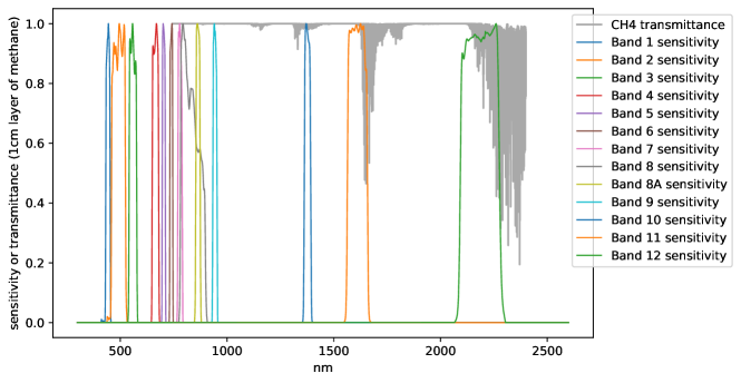
Figure 1: Methane transmittance spectrum and Sentinel-2 A spectral sensitivity for all its bands. Ignoring the cirrus band B10 that is not suitable for monitoring applications, only bands B11 (1568-1659 nm) and B12 (2114-2289 nm) are impacted by the presence of methane in the atmosphere. The other bands are not impacted.

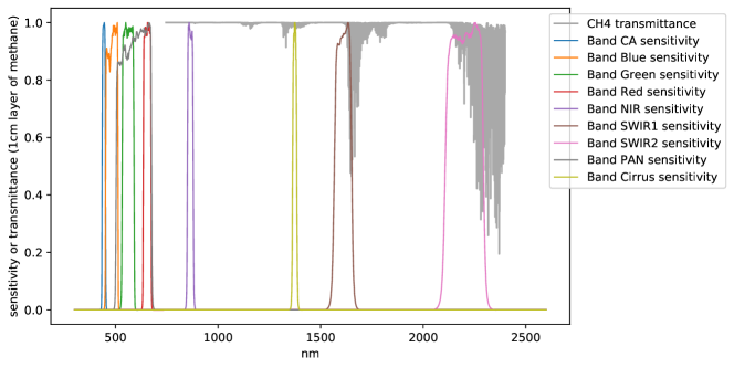
Figure 2: Methane transmittance spectrum and Landsat-8 spectral sensitivity for all its bands. Similarly to Sentinel-2, the two SWIR bands SWIR1 and SWIR2 can be used for methane detection and quantification.

We use a simple absorption model to characterize the attenuation due to the presence of methane. The Beer-Lambert law states that for a light source with intensity $I_{0}$ and a wavelength $\lambda$

$$I=I_{0}e^{-\sum_{i=0}^{N}A_{i}(\lambda)l_{i}},$$ (1)

where the light goes through $N$ gases defined by their absorption $A_{i}(\lambda)$ and equivalent optical path length $l_{i}$ defined as the product of the actual optical path and the concentration of the i${}^{\text{th}}$ gas. In our case, the $N$ gases correspond to the atmosphere and $I_{0}$ is the sunlight in the SWIR spectrum. We can also reasonably assume $I_{0}$ to be constant for all wavelengths $\lambda$ in each band respectively. Taking into account that the sensor of a satellite integrates over a band of wavelengths described by a sensitivity function $s$, the intensity of the light seen by a space-borne sensor becomes

$$I=I_{0}\int s(\lambda)\alpha(\lambda)e^{-\gamma\sum_{i=0}^{N}A_{i}(\lambda)l_{i}}d\lambda,$$ (2)

where the two passes through the atmosphere are taken into account in $\gamma$ (which is a function of both the sun azimuth angle and the satellite view angle). The reflection coefficient of the ground is represented in the formula by the surface albedo $\alpha(\lambda)$. See Fig. 3.

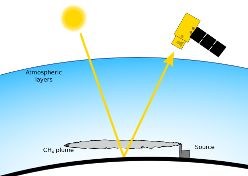
Figure 3: Atmosphere observation model. The on board sensor sees the light coming from the sun after reflection on Earth. Its intensity has dimmed due to the atmosphere and the reflection process. The dimming is also impacted by the presence of a methane plume.

In the presence of a methane emission, characterized by $l_{leak}$, the intensity of the light seen by the sensors becomes

$$I_{leak}=I_{0}\int s(\lambda)\alpha(\lambda)e^{-\gamma\sum_{i=0}^{N}A_{i}(\lambda)l_{i}}e^{-\gamma A_{CH4}(\lambda)l_{leak}}d\lambda.$$ (3)

Supposing that we have both the exact same observation with and without a methane emission, it becomes very easy to detect the emission. Indeed $I_{leak}<I$ everywhere $l_{leak}$ is non zero. The problem is that the observation without methane, also called background observation, is never available in practice. Therefore, a reference observation without methane is needed in order to distinguish an attenuation due to the presence of methane from a difference in the surface albedo.

When we assume that methane emissions are anomalous events, it is to be expected that most observations in a time series should not contain excess methane. So, if we suppose that the surface albedo is rather stable in time, the time series can be used to estimate a methane free background model that can be compared with the current observation. Here, we compute the background for a given date as its linear regression over the previous dates. If we denote by $I_{t}$ the observation at time $t$, then the regression computes the optimal weights $w_{i}$ that solve

$$\min_{\{w_{i}\}}\left\|I_{t}-\sum_{i=0}^{t-1}w_{i}I_{i}\right\|^{2}.$$ (4)

Then the background is obtained as the linear combination $\sum_{i=0}^{t-1}w_{i}I_{i}$. To further improve the background subtraction we combine this estimation with a band ratio that exploits the correlation between SWIR bands, similarly to the multiple-band single-pass (MBSP) from Varon et al. ²².

Quantifying emissions is also an important part of monitoring. While the previous processing was presented for methane emission detection, it can also be used to quantify it. Supposing that both the signal with the emission $I_{leak}$ and without emission $I_{bg}$ are available (using for example the process presented previously), then

$$\frac{I_{leak}}{I_{bg}}\approx\frac{\int_{B12}s(\lambda)e^{-\gamma\sum_{i=0}^{N}A_{i}(\lambda)l_{i}}e^{-\gamma A_{CH4}(\lambda)l_{leak}}d\lambda}{\int_{B12}s(\lambda)e^{-\gamma\sum_{i=0}^{N}A_{i}(\lambda)l_{i}}d\lambda}.$$ (5)

Since $\gamma$ is known for each acquisition, this ratio only depends on the atmosphere composition. Therefore, for a fixed atmosphere composition, it is possible to estimate the value of $l_{leak}$ as the solution of a simple optimization problem

$$\operatorname*{arg\,min}_{l_{leak}}\left\|\frac{I_{leak}}{I_{bg}}-\frac{\int_{B12}s(\lambda)e^{-\gamma\sum_{i=0}^{N}A_{i}(\lambda)l_{i}}e^{-\gamma A_{CH4}(\lambda)l_{leak}}d\lambda}{\int_{B12}s(\lambda)e^{-\gamma\sum_{i=0}^{N}A_{i}(\lambda)l_{i}}d\lambda}\right\|^{2}_{2}.$$ (6)

In practice, the atmosphere model can be well approximated with a simple “pure methane atmosphere”, i.e. an atmosphere that’s purely made of methane, instead of considering a complete atmosphere model. This quantification scheme can also be adapted when using band ratio.

4 Practical methane emission tracking

We present in this Section the practical implementation of the detection and quantification principles mentioned in the previous section. Namely, we first present the different preprocessing steps necessary for the method to function. We provide more details about the background reconstruction process, the detection validation process and the quantification process. This practical methodology is the one used to perform all the experiments presented in this paper. Fig. 4 illustrates the different steps of the proposed methodology for Sentinel-2; Fig. 5 illustrates the same steps but for Landsat-8.

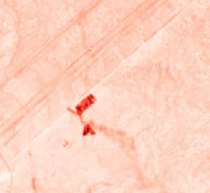
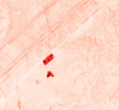
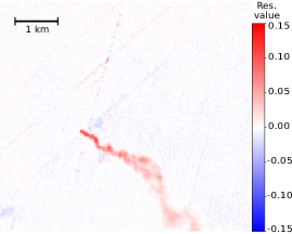
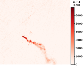
Figure 4: Visualization of each step of the detection and quantification method. From left to right, top to bottom: the Sentinel-2 image of the location (only the RGB channels are shown), the log band ratio corresponding to the image, the predicted background model, the residual showing the plume, the mask corresponding to the detected plume and the associated quantification in ppb.

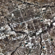
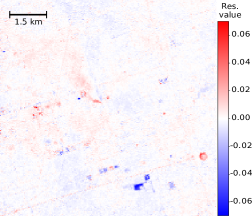
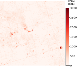
Figure 5: Visualization of each step of the detection and quantification method. From left to right, top to bottom: the Landsat-8 image of the location (only the RGB channels are shown), the log band ratio corresponding to the image, the residual showing the plume, the mask corresponding to the detected plume and the associated quantification in ppb.

4.1 Preprocessing

From now on, we consider areas of interest of size approximately 10x10 km². We found out that this size is well adapted to capture methane plumes created by emissions, while being large enough so that the reconstruction is not impacted too much by the presence of methane in the reference images. We collect L1C Sentinel-2 timeseries corresponding to the areas of interest, preferably considering timeseries longer than six months. We first co-register all the images of a timeserie using the method by Hessel et al. ²³. We also apply a cloud detection algorithm, such as the one proposed by Dagobert et al. ²⁴, to estimate the cloud cover. All images with more than $15\%$ of the pixels covered by clouds are discarded. Sentinel-2 images comprise $12$ bands with spatial resolutions from $10$m per pixel to $60$m per pixel. The two bands of interest, namely band 11 and band 12, are both sampled at $20$m per pixel therefore there is no need for resampling them. However, we have observed that these two bands are aliased. This is particularly important because we are computing ratios of these two bands and therefore this aliasing can create large artifacts during the processing (see Fig. 6). In order to avoid this problem we apply an anti-aliasing filter, namely a Gaussian filter with parameter $\sigma=0.7$, prior to any other processing. We also apply a log on the ratio. This limits the impact on the reconstruction of abnormal high values present in the SWIR bands, for example due to flaring, which are frequently found in the vicinity of oil and gas facilities. As it will be seen in the Detection validation subsection, the other bands are still useful to validate a plume detection. This is why we resample all these bands to $20$m per pixel so that comparison is easier.

(a) Band 12 of Sentinel-2 to align everything

(b) Ratio between B12 and 11 without an antialiasing filter

(c) Ratio between B12 and 11 with an antialiasing filter

Figure 6: Eventhough it is barely visible, Sentinel-2 images are aliased and therefore should be preprocessed before computing the ratio. The artifacts due to aliasing would impact the processing otherwise. A Gaussian filter with parameter $\sigma=0.7$ allows to remove this aliasing before the processing. Figure best seen zoomed.

4.2 Background estimation

The core of the detection method is the background estimation process. For that, each time-series of log band ratios computed above is processed using a sliding window of size $T=30$ dates. For each date in the window, we compute its linear projection on the past $T-1$ images. Using the estimated background, we define a residual that corresponds to the difference between the input data and the prediction. A longer time series improves the SNR of the extracted plume, thus fostering its detection ²⁵. Note that by projecting on a time series there is no need to manually choose a reference date as background ²².

Similarly to how flaring could impact the background estimation, new (or disappearing) large structure can also lead to errors in the quantification. To limit the impact of outliers, robust estimation methods such as Huber regression ²⁶ or the iteratively reweighted least square algorithm ²⁷ can be used. We found out that in our case such robust regression methods are quite slow. For this reason, we use an approximate two-steps estimation method that is good enough for this application. A first estimation is done using a linear projection as presented previously. Then the $5\%$ of pixels with the worst estimation are discarded. The remaining pixels are then used to perform a second linear projection, this time without the outliers. The coefficients estimated with the second linear projection are used to perform the final estimation. We argue that even if pixels containing methane are initially discarded, this is not a problem because methane should, by definition, not impact the background prediction. Fig. 7 shows a case in which this procedure allows to refine the background reconstruction. The reconstruction error of the background is almost twice as small when using a two step estimation.

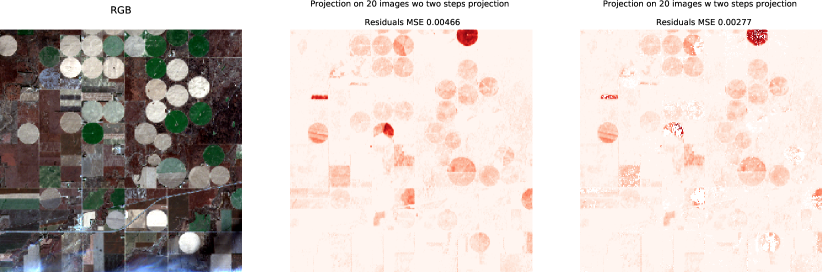
Figure 7: Improvement of background estimation when using a two-steps estimation. Left to right: The RGB image of the scene, the background estimated using a single step, the background estimated using two steps. Using two steps allows to have a much smaller MSE than a single step estimation (with the outliers set to zero). The MSE has been estimated on the same pixels (i.e. without the outliers) for both images.

Despite removing outliers, the two-stage approach cannot deal with time series containing large zones with changing albedo. This is the case for the crop fields seen in Fig. 8, for which a spatially adaptive processing must be adopted. The objective is to bring non linearity to the projection by performing one projection for each zone of similar albedo. An albedo map is computed by clustering the pixels of our images with four different features: the temporal standard deviation and median of the absorbing band, the $x$ and $y$ position of the pixel in the image. The clustering is done using a Gaussian mixture model, and the optimal number of clusters is fixed with the post analysis of the Bayesian information criterion of the clustering ²⁸. This methodology being more computationally intensive is performed only on regions with a high albedo variance such as regions with many crop fields as shown Figure 8.

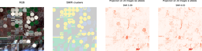
Figure 8: Improvement of background estimation when using clustering. Left to right: The RGB image of the scene, the different clusters estimated from the albedo, the background estimated without the clusters, the background estimated with the clusters. Using a clustering step during the background estimation increases the SNR of the methane plume with respect to the background.

4.3 Detection validation

While we would like to have a completely automatic detection process, directly detecting on the residuals computed in Background estimation yielded too many false detections. This is why we added an extra step where all detections are done and verified manually. In particular, a mask corresponding to the shape of the potential plume is first manually annotated. We then compare the content of the annotated region to the content of the same region but in the other bands. If the potential plume is indeed a true methane plume, then it should not be correlated to the content of the bands that are not impacted by the presence of methane. In particular, a similar shape should not be found in these other bands. Some surfaces, for example snow, have a higher reflectance in B11 than B12. This causes a contrast inversion and a dimming-like phenomenon when looking at the band ratio. Because of that, it is possible that potential plumes appear in the band ratio even though they do not correspond to an actual dimming in B12. The last validation step checks that the detection corresponds indeed to a dimming in B12.

4.4 Source quantification

Once the mask of the plume is available, we quantify the emission rate corresponding to the source of the plume. The first step is to quantify the equivalent amount of methane $l_{CH4}$ per pixel that corresponds to the extra methane attributed to the source. For that, we adapt the quantification model presented in Eq. 6 so as to take into account the extra log preprocessing as well as the band ratio. This leads to an excess of methane $\Delta\Omega(p)$ for the pixel $p$ corresponding to

$$\footnotesize\Delta\Omega(p)=\operatorname*{arg\,min}_{l_{leak}}\left\|R(p)-\log\left(\frac{\int_{B12}s(\lambda)e^{-\gamma A_{CH4}(\lambda)(l_{atm}+l_{leak})}d\lambda}{\int_{B12}s(\lambda)e^{-\gamma A_{CH4}(\lambda)l_{atm})}d\lambda}\frac{\int_{B11}s(\lambda)e^{-\gamma A_{CH4}(\lambda)l_{atm})}d\lambda}{\int_{B11}s(\lambda)e^{-\gamma A_{CH4}(\lambda)(l_{atm}+l_{leak})}d\lambda}\right)\right\|^{2}_{2},$$ (7)

with $R(p)$ the estimated residual at pixel $p$ and $l_{atm}$ the amount of methane naturally present in the atmosphere. We define $l_{atm}$ such that it corresponds to a residual background of $1800$ppb of methane. In practice, while the specific background level might fluctuate depending on the location and time, the error due to this approximation for the estimation of the excess of methane is negligible compared to all other sources of uncertainty (see ²⁹). To estimate $A_{CH4}$, we use the HITRAN database ³⁰. We also use the sensitivity $s$ of Sentinel-2 A, respectively Sentinel-2 B, calibrated in laboratory provided by ESA (https://sentinels.copernicus.eu/web/sentinel/technical-guides/sentinel-2-msi/performance). The optimization is done using the downhill simplex algorithm.

Once each pixel of the plume has been quantified, we estimate the source emission rate using the integrated mass enhancement (IME) method ³¹. The IME method relates the source rate $Q$ to the total detected plume mass by

$$Q=A\frac{U_{eff}}{L}\sum_{p\in\mathcal{M}}\Delta\Omega(p),$$ (8)

where $U_{eff}$ corresponds to the effective wind speed, $L$ the plume length, $\mathcal{M}$ the mask of the plume, $A$ the area covered by a pixel (in this case $A=400\text{m}^{2}$). Similarly to Varon et al. ³¹, we estimated $L$ using the plume mask $M$ such that $L=\sqrt{A\times\#M}$ with $\#M$ the number of pixels in the plume mask $M$. We use wind data collected from the ECMWF-ERA5 reanalysis product from the Copernicus Climate Change Service ³². Varon et al. ³¹ showed that $U_{eff}$ can be related to the local wind speed at 10m $U_{10}$ therefore we select the wind product at 10m above ground level and at the closest time before the sensing time for each estimation. The source origin is selected manually using jointly the wind data and the plume shape.

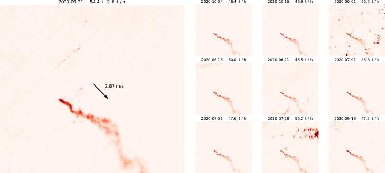
Figure 9: The uncertainty of the plume on the left is estimated by simulating the same plume in other images of the timeseries. Each estimated plume (in ppb) as well as their predicted emission rate are shown on the right. The arrow corresponds to the wind information used for the emission rate quantification.

Note that, in the following, Sentinel-5P measurements are not estimated using this process. They are instead derived from the methane concentrations provided by the Level-2 methane product. For that, we estimate a background methane concentration, by computing the median methane concentration neighboring a plume in the Level-2 product, which we remove from the measurements so that only the excess methane is measured.

4.5 Quantifying the uncertainty caused by the proposed background removal method

Different factors can contribute to quantification errors in the proposed method. We focus here on the uncertainty induced by the proposed background estimation method by providing a per-scene uncertainty estimation. Note that the error estimated here does not include the uncertainty due to the IME process, the two need to be combined to obtain the final uncertainty corresponding to the source emission.

Fluctuations in the albedo and atmospheric conditions might be wrongly quantified as excess of methane. The idea is to estimate the quantification errors due to these fluctuations by simulating the same methane plume in other images of the time series: From each new simulated image the quantification method is run again and a new emission rate is estimated. The uncertainty is then obtained as the standard deviation of the emission rates estimated with the simulated images. Fig. 9 illustrates the concentrations obtained by applying this procedure on different images of a time series.

5 Validation of the proposed methodology: the September 2020 Permian event

We applied the proposed methodology to estimate emission rates during an event in the Permian basin. This event occurred during the summer of 2020 (estimated latitude and longitude of the source: (31.7335, -102.0421)) and lasted about two months. Several observations from Sentinel-2, Landsat-8, Sentinel-5P were collected and airborne hyperspectral observations from previous campaigns are available. The airborne measurements were obtained in September 2020 (towards the end of the event) with Scientific Aviation flights and are provided by the PermianMap project (Operator Performance Dashboard: data from U. Arizona, NASA-JPL, and EDF provided via the PermianMap project by EDF (https://data.permianmap.org/pages/operators). Users are bound by the Terms of Use of this data).

Fig. 10 shows the estimated emission rates from the mentioned sources. As we can see, the emission measurements of the airborne campaign and all those obtained after September 15${}^{\text{th}}$ 2020 seems to be close and consistent with each other up until the last two EDF measurements. Yet, the analysis of the time series leads to conclude that the event had started two months prior to the aircraft campaign, thus increasing significantly the total amount of CH₄ released. Note that the measurements as well as the estimated confidence intervals are consistent. Since no emissions were detected before July 9${}^{\text{th}}$ 2020 or after September 29${}^{\text{th}}$ 2020, these measurements enable a full description of the event from start to end. Given that we observed a methane plume at each of the 12 dates where Sentinel-2 and Landsat-8 images were available (the plumes are shown in Fig. 11), we assume that this event is continuous. Indeed, if that source was intermittent, we would have observed random peaks before or after our period of interest or dates with no emissions. We can therefore interpolate linearly the emission rate at a date with no image available using the two closest emission rates available. This leads to an estimation of a grand total of 16,537±7,146 tons of methane emitted during this event.

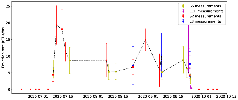
Figure 10: Emission rates measured during an event in the Permian basin occurred during the summer of 2020 (estimated latitude and longitude: 31.7335, -102.0421). The plot combines estimates obtained from Sentinel-2, Landsat-8, Sentinel-5P and from Scientific Aviation flights (with their respective uncertainty corresponding to the standard deviation of the estimates). All of these estimates show that the emission started more than two months earlier than it was initially reported by the EDF campaign. Moreover, these estimates seems to be consistent across sources.

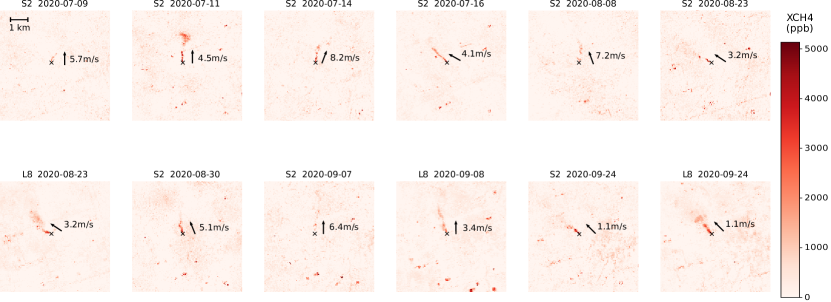
Figure 11: Illustration of the plumes (in ppb) observed using Sentinel-2 (S2) and Landsat-8 (L8) imagery during the event in the Permian basin occurred during the summer of 2020 (estimated latitude and longitude: 31.7335, -102.0421) studied in Fig. 10. The source of the emission is located at the center of the images (symbolized by the black cross) and the wind information is represented by the arrow.

6 Results

We monitored about 7000 geographical sites of interest linked to oil and gas facilities during a period of 47 months, from November 2017 to September 2021. Every site is associated to a 10x10km tile. For every tile, a time series of at least six months was extracted. In total for this study, more than 1248621 (potentially cloudy) tiles were processed over 562652 km². The proposed dataset comprises a location and a quantification for all plumes. Each detected plume in the dataset is quantified using the IME method (see the Source quantification subsection). Fig. 12 shows a selection of methane plumes from the proposed dataset. We also associate to each plume the corresponding wind data from ECMWF-ERA5 ³² that is used to quantify the emission.As of September 2021, 1202 plumes were detected using Sentinel-2 images from 92 different sites of interest, mostly located in three countries: Algeria, Turkmenistan and the United States (see Fig. 14). Table 1 shows the number of detected events per country. Note that the imbalance of detection in the US compared to the Algeria in the proposed dataset is mostly due to more difficult sensing conditions. Indeed, it was shown by Gorroño et al. ³³ through simulations that the detection limit of Sentinel-2 can be expected to be in the 8 to 12 t${}_{\text{CH}_{4}}$/hr in the Permian basin in the US while it should be in the 1.5 to 2.5 t${}_{\text{CH}_{4}}$/hr range in Turkmenistan. We empirically verified these expected detection limits through our detections with Sentinel-2.

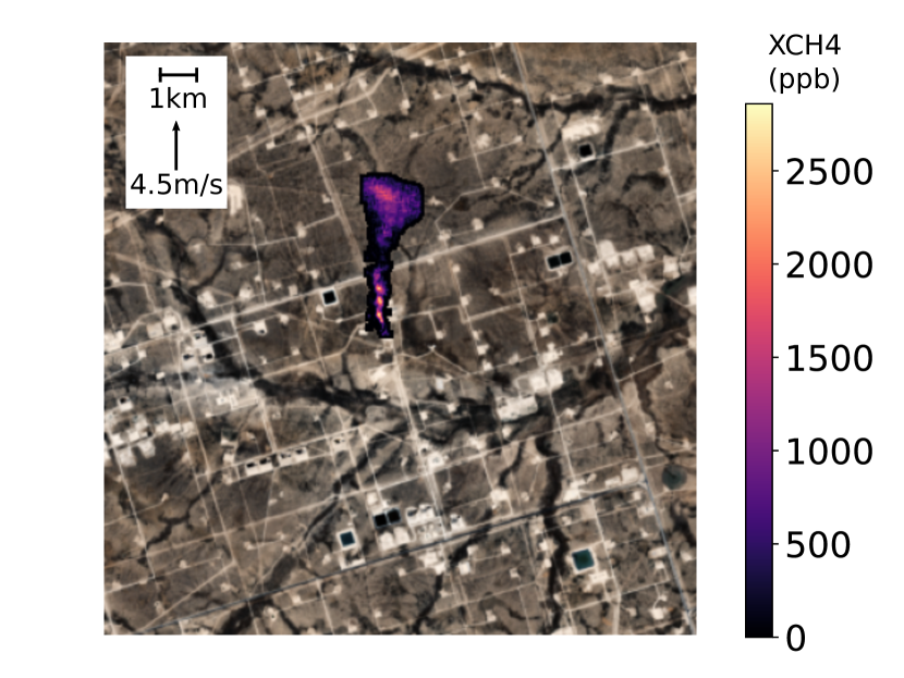
(a) US, 14.5 t${}_{\text{CH}_{4}}$/hr

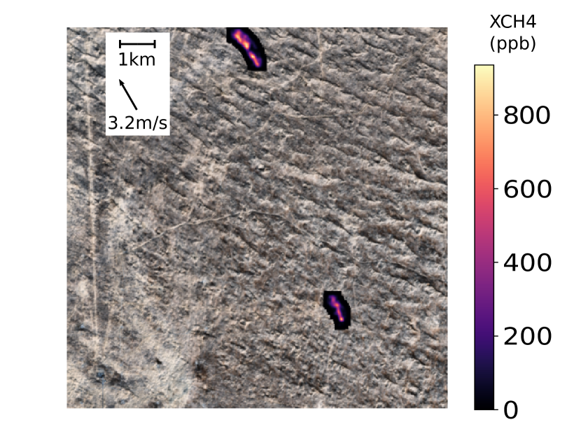
(b) Turkmenistan, 8.7 t${}_{\text{CH}_{4}}$/hr

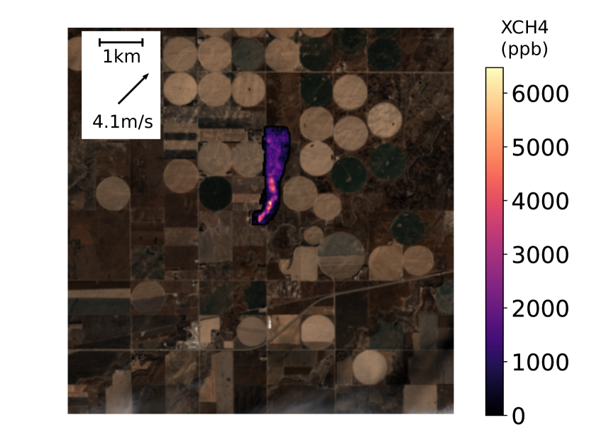
(c) US, 54 t${}_{\text{CH}_{4}}$/hr

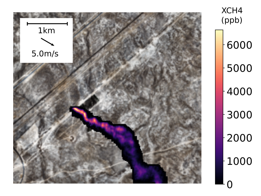
(d) Kazakhstan, 62.8 t${}_{\text{CH}_{4}}$/hr

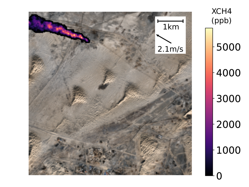
(e) Turkmenistan, 41 t${}_{\text{CH}_{4}}$/hr

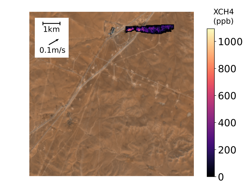
(f) Algeria, 3.1 t${}_{\text{CH}_{4}}$/hr

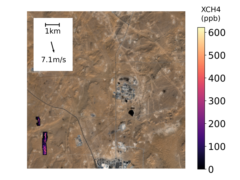
(g) Algeria, 5.7 t${}_{\text{CH}_{4}}$/hr

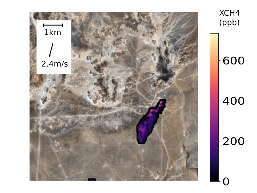
(h) Algeria, 3.3 t${}_{\text{CH}_{4}}$/hr

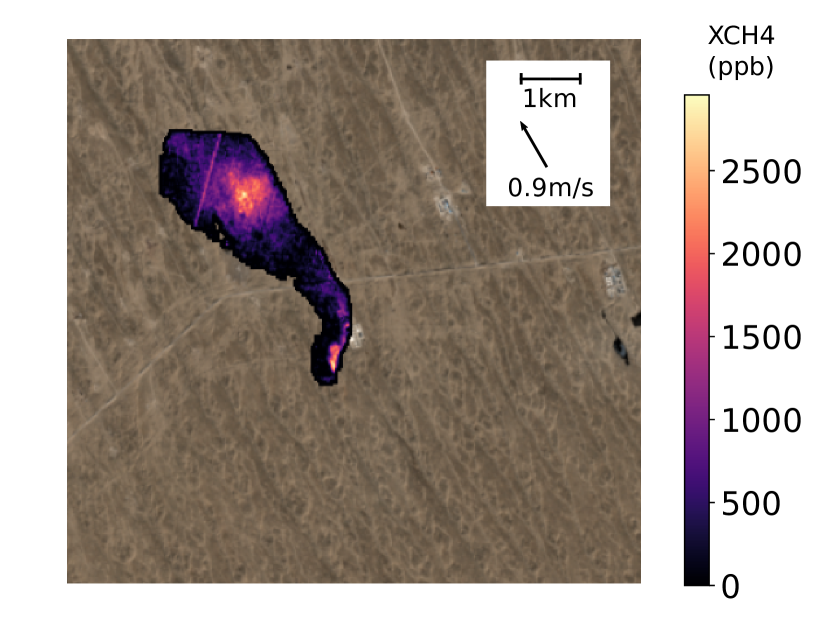
(i) Turkmenistan, 27.5 t${}_{\text{CH}_{4}}$/hr

Figure 12: Examples of detected plumes over oil and gas facilities. The plume is shown as a white and purple mask over the corresponding Sentinel-2 satellite RGB images (top of atmosphere). Wind information is represented by the arrow.

We then classified these emissions into two main categories: recurrent and unique. An event is said to be recurrent when at least two methane plumes have been detected in the time series of a given area of interest. The rest of the emission are characterized as unique i.e. only one plume was detected in the considered area of interest in the entire time series. We found that $58\%$ of these plumes could be attributed to recurrent events. This means that these events are likely not due to an unexpected major incident, and could probably be avoided with better monitoring and maintenance of oil and gas facilities. We present a more detailed histogram of recurrence of emissions in Fig. 13.

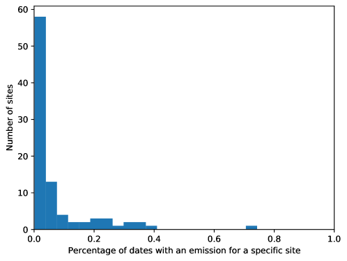
Figure 13: Histogram of recurrence of emissions.

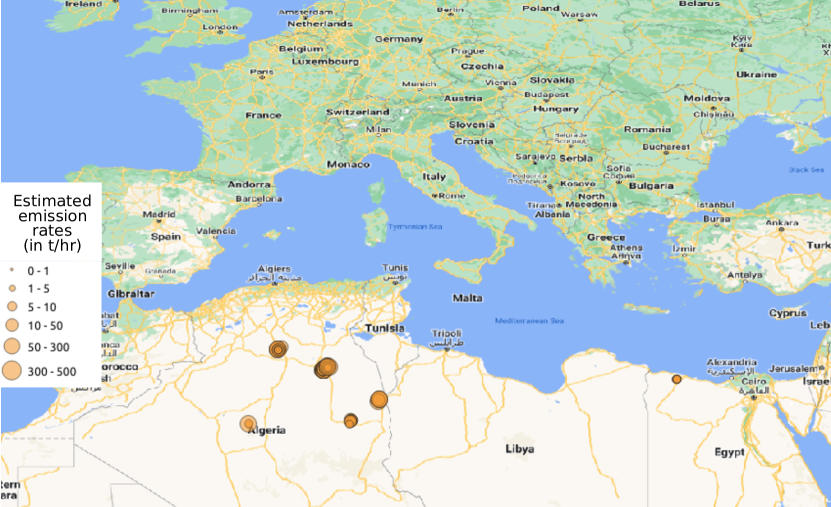
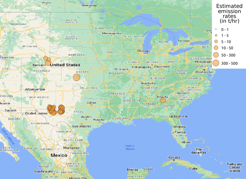
(b) Location of the plumes detected in the Algeria region. (c) Location of the plumes detected in the US.

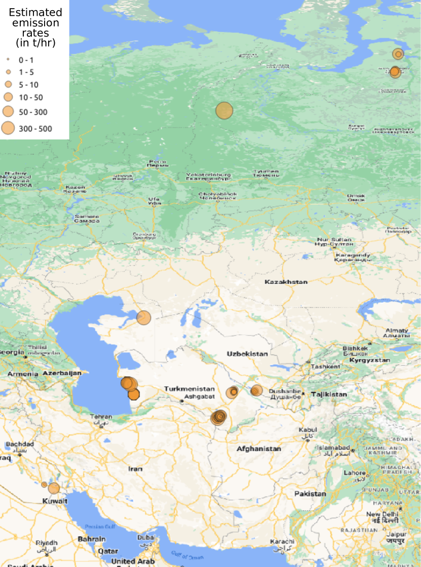
(a) Location of the plumes detected in the Turkmenistan region.

Figure 14: Locations of the different detected emissions corresponding to the proposed dataset. The quantified emission rates are illustrated by the circles’ diameter.

Country	Number of events
Algeria (DZA)	527
Turkmenistan (TKM)	526
United States (USA)	98
Uzbekistan (UZB)	27
Egypt (EGY)	13
Russian Federation (RUS)	7
Iraq (IRQ)	3
Kazakhstan (KAZ)	1

Table 1: Distribution by country of the detected emissions during the period of 47 months going from November 2017 to September 2021.

6.1 Global power law fitting

Power law models have been shown to be a good fit for many GHG emission studies ^{34, 35, 36}. In a recent paper, Lauvaux et al. ¹⁵ postulated that the methane emission events follow a power law distribution at a global scale. This was observed using emission rates estimated from Sentinel-5P and airborne hyperspectral measurements. In this work, we merged the events from our Sentinel-2 based dataset into the previously proposed power law plot ¹⁵ to complete the picture. The power law that we obtained is shown in Fig. 15. We rescaled counts for Sentinel-2 and airborne campaigns so that counts match for all sources for emissions rates where events can be detected by multiple sources. The rationale behind this scaling is that, everything else being equal, detection counts should match for all sources for which emission rates are above the detection limit. The scaling is thus meant to compensate for differences in spatial coverage, revisit frequency, weather impact, etc. This is justified by the study of the Permian event where we show that given the proper sensing conditions detections match across the different source type considered here. In practice, this means that Sentinel-2 counts are scaled to match Sentinel-5P counts at 50 t${}_{\text{CH}_{4}}$/hr, while California ² and Permian ⁸ airborne campaigns counts are scaled to match S2 counts at 5 t${}_{\text{CH}_{4}}$/hr. For that, the regressions are first estimated for each source independently and the scaling is then done based on the estimated regression by changing the intercept to ones that align the different models. For example, consider that the detections from Sentinel-5P can be modeled using $\beta_{S5}x^{\alpha_{S5}}$ and the detections from Sentinel-2 by $\beta_{S2}x^{\alpha_{S2}}$. In that case, the scaling for Sentinel-2 corresponds to $\beta_{S2,scale}=\beta_{S5}x_{S2,S5}^{\alpha_{S5}-\alpha_{S2}}$ where $x_{S2,S5}=50t_{\text{CH}_{4}}/hr$ as mentioned previously. This means that the scaled model for Sentinel-2 coincides with the model for Sentinel-5P in $x_{S2,S5}=50t_{\text{CH}_{4}}/hr$ but the slope of the model is not changed.

We define the detection limit as the threshold that represents the regime in which, except in the most adverse conditions, sources should be detected. In practice, it corresponds to the point below which the linear models is not valid anymore since detections are missed. This phenomenon is visible in Fig. 15 where each curve “tails off” on the lower end. This also means that it is possible to detect emissions smaller than this limit when conditions are optimal (e.g appropriate wind conditions, good atmospheric conditions and good surface reflectance). In order to have more robust models, the estimation of the power laws is done using only the data above their detection limits.

It also seems that there is a maximum detection limit for Sentinel-2. We think that it is just because, in practice, these events are rare. Sentinel-5P is capable of detecting very small excesses of methane – over a large spatial region – thanks to its hyperspectral sensor. As such, it is able to detect a plume even – closely – after the end of an event. On top of that it provides a large spatial coverage and better revisit frequency. In the end, it is much more likely to find ultra-emitters with Sentinel-2 than Sentinel-5P and this explains the apparent maximum detection limit in Fig. 15. It is also possible that some of these events have been under-quantified because of the difficulty to annotate very large events (similarly to how it is difficult to quantify properly ultra-emitters with airborne campaigns).

Remark that Sentinel-2 observations are well aligned with the Sentinel-5P power law slope and complete the range for medium scale events, bridging the gap in emission rates between small sources (0.1 t${}_{\text{CH}_{4}}$/hr to 10 t${}_{\text{CH}_{4}}$/hr) captured by airborne campaigns and the ultra-emitters ($>$ 25 t${}_{\text{CH}_{4}}$/hr) detected by, for example, Sentinel-5P. This shows that at a global scale large event observations seen by Sentinel-5P are a good proxy indicator for smaller events in the range covered by Sentinel-2 (i.e. $>$ 25 t${}_{\text{CH}_{4}}$/hr) showed in green in Fig. 15. The good alignment with the data from the airborne campaign hints that the model might still be valid for even smaller events in the range covered by these campaigns (i.e. $>$ 0.1 t${}_{\text{CH}_{4}}$/hr) showed in gray in Fig. 15. It is however unlikely that the power-law is still valid for even smaller events corresponding to the last region shown in red in Fig. 15. There exists a theoretical limit to the power law that has not been identified yet. Most likely, once observing small leaks from pressure valves, it is expected to see a major shift in the distribution.

Our results suggest that one could only monitor the largest emitters and draw conclusions on smaller emitters, assuming that the slope is defined by structural variables (for example the ratio between small and large pipes) and by the maintenance operation procedures. Assuming that the slope of the power law will remain, one could track progress by only looking at a fraction of the top emitters and extrapolate the observed trend to smaller emitters. While the statistical relationship (Power Law) observed across our data set suggests that large emitters offer indirect monitoring of smaller emitters, the linear coefficients from such regression will be specific to each producing region. Additional data are necessary to constrain more precisely the slopes of regional Power Law relationships.

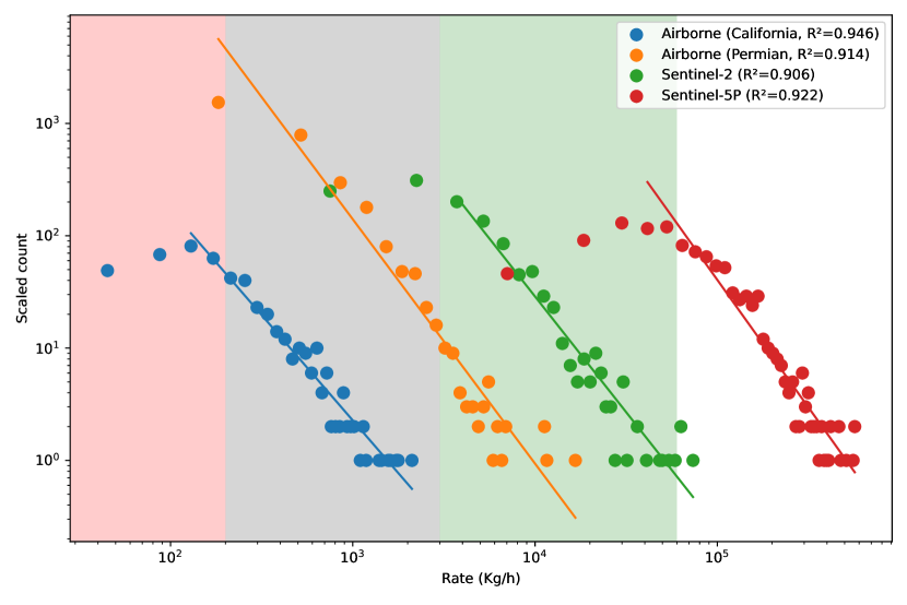
(a) Before scaling

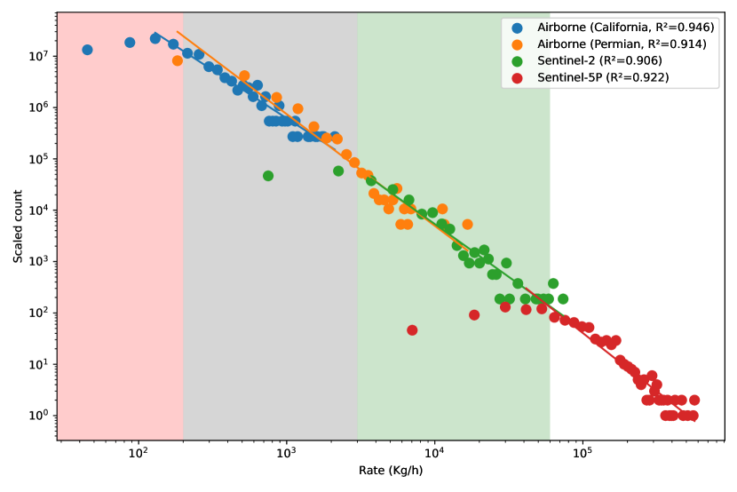
(b) After scaling

Figure 15: Power law plot of Sentinel-5P and Sentinel-2 events, together with airborne campaigns over California ² and the Permian ⁸. Counts are scaled to match in common detection zones. Since data is consistent across the different sources used for the study, this shows that at a global scale large event observation might be a good proxy indicator for smaller but unobserved events (corresponding to the green region). The grey region represent the region where the model still be valid. It is however unlikely that the power law model is still valid in the red region.

6.2 Per country analysis

We analyzed the previous data on a per-country basis. We considered only measurements from Sentinel-5P and Sentinel-2 and studied the detections in Algeria and Turkmenistan. This analysis is shown in Fig. 16. Extending the global power law presented previously, these two countries exhibit a similar power law model at a regional level. This means that not only ultra-emitters ($>$ 25 t${}_{\text{CH}_{4}}$/h) are a proxy to large-emitters ($>$ 2 t${}_{\text{CH}_{4}}$/h) at a global scale, they might also be a good proxy at a more local, e.g. basin, level.

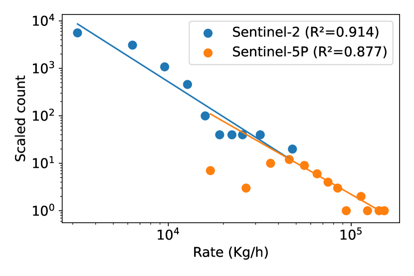
(a) Local power law for the region of Algeria. additional text

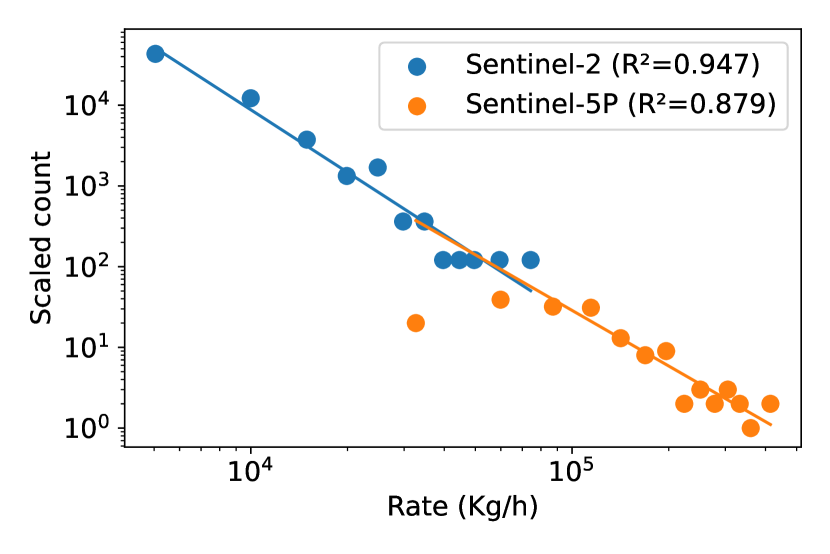
(b) Local power law for the region of Turkmenistan.

Figure 16: Power law by country using Sentinel-2 and Sentinel-5P measurements. This seems to indicate the power law is still valid at a regional level. Left: Algeria, right: Turkmenistan

We performed the same analysis with Sentinel-2 and airborne measurements in the Permian bassin basin in the US. This power law is presented in Fig. 17. Once again, the power law model seems to be valid at this local regional level. It seems to indicate that the hypothesis such that Sentinel-2 could be a good proxy indicator for airborne measurements done for the global law power is indeed valid.

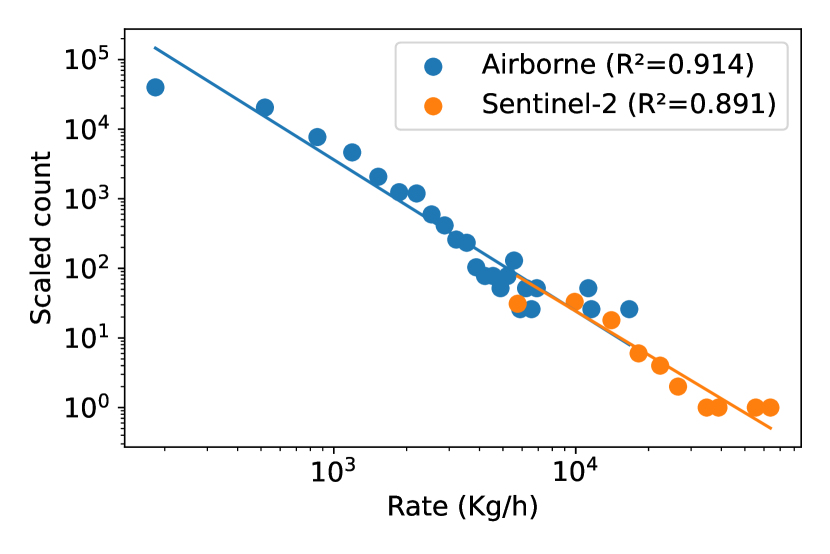
Figure 17: Local power law for the Permian basin in the US using Sentinel-2 and airborne ⁸ measurements. This seems to validate the hypothesis that Sentinel-2 is also a proxy indicator for smaller events corresponding to the ones detected by the airborne campaign.

7 Supporting Information

Plume list with localization and quantification (XLSX)

The authors thank Omar Dhobb from Kayrros for his encouragement and support and acknowledge Edouard Machover for his early work on this subject. Work partly financed by Office of Naval research grant N00014-17-1-2552, DGA Astrid project “Filmer la Terre” n^o ANR-17-ASTR-0013-01, and MENRT. T. Lauvaux was supported by the French research program “Make Our Planet Great Again” (CNRS, project CIUDAD). Alexandre d’Aspremont is at CNRS & département d’informatique, École normale supérieure, UMR CNRS 8548, 45 rue d’Ulm 75005 Paris, France, INRIA and PSL Research University, and would like to acknowledge support from the ML and Optimisation joint research initiative with the fonds AXA pour la recherche and Kamet Ventures, a Google focused award, as well as funding by the French government under management of Agence Nationale de la Recherche as part of the ”Investissements d’avenir” program, reference ANR-19-P3IA-0001 (PRAIRIE 3IA Institute).

References

- Brandt et al. 2014 Brandt, A. R. et al. Methane leaks from North American natural gas systems. Science 2014, 343, 733–735
- Duren et al. 2019 Duren, R. M. et al. California’s methane super-emitters. Nature 2019, 575, 180–184
- McKeever et al. 2019 McKeever, J.; Jervis, D.; Strupler, M.; Gains, D.; Tarrant, E.; Varon, D. J.; Maasakkers, J. D.; Pandey, S.; Houweling, S.; Aben, I.; Scarpelli, T.; Jacob, D. Detection and Imaging of Methane Emissions Plumes from Oil and Gas Facilities with GHGSat-D. AGU Fall Meeting Abstracts. 2019; pp GC51M–0962
- Varon et al. 2019 Varon, D.; McKeever, J.; Jervis, D.; Maasakkers, J.; Pandey, S.; Houweling, S.; Aben, I.; Scarpelli, T.; Jacob, D. Satellite discovery of anomalously large methane point sources from oil/gas production. Geophysical Research Letters 2019, 46, 13507–13516
- Zhang et al. 2020 Zhang, Y. et al. Quantifying methane emissions from the largest oil-producing basin in the United States from space. Science Advances 2020, 6, eaaz5120
- Guha et al. 2020 Guha, A. et al. Assessment of Regional Methane Emission Inventories through Airborne Quantification in the San Francisco Bay Area. Environmental Science & Technology 2020, 54, 9254–9264
- Irakulis-Loitxate et al. 2021 Irakulis-Loitxate, I. et al. Satellite-based survey of extreme methane emissions in the Permian basin. Science Advances 2021, 7, eabf4507
- Cusworth et al. 2021 Cusworth, D. H.; Duren, R. M.; Thorpe, A. K.; Olson-Duvall, W.; Heckler, J.; Chapman, J. W.; Eastwood, M. L.; Helmlinger, M. C.; Green, R. O.; Asner, G. P.; Dennison, P. E.; Miller, C. E. Intermittency of large methane emitters in the Permian Basin. Environmental Science & Technology Letters 2021, 8, 567–573
- Forster et al. 2021 Forster, P.; Storelvmo, T.; Armour, K.; Collins, W.; Dufresne, J.-L.; Frame, D.; Lunt, D.; Mauritsen, T.; Palmer, M.; Watanabe, M.; Wild, M.; Zhang, H. In Climate Change 2021: The Physical Science Basis. Contribution of Working Group I to the Sixth Assessment Report of the Intergovernmental Panel on Climate Change; Intergovernmental Panel on Climate Change,, Ed.; Cambridge University Press, 2021
- Lyon et al. 2016 Lyon, D. R.; Alvarez, R. A.; Zavala-Araiza, D.; Brandt, A. R.; Jackson, R. B.; Hamburg, S. P. Aerial surveys of elevated hydrocarbon emissions from oil and gas production sites. Environmental science & technology 2016, 50, 4877–4886
- Veefkind et al. 2012 Veefkind, J. et al. TROPOMI on the ESA Sentinel-5 Precursor: A GMES mission for global observations of the atmospheric composition for climate, air quality and ozone layer applications. Remote sensing of environment 2012, 120, 70–83
- Pandey et al. 2019 Pandey, S.; Gautam, R.; Houweling, S.; van der Gon, H. D.; Sadavarte, P.; Borsdorff, T.; Hasekamp, O.; Landgraf, J.; Tol, P.; van Kempen, T.; Hoogeveen, R.; van Hees, R.; Hamburg, S. P.; Maasakkers, J. D.; Aben, I. Satellite observations reveal extreme methane leakage from a natural gas well blowout. Proceedings of the National Academy of Sciences 2019, 116, 26376–26381
- Schneising et al. 2020 Schneising, O.; Buchwitz, M.; Reuter, M.; Vanselow, S.; Bovensmann, H.; Burrows, J. P. Remote sensing of methane leakage from natural gas and petroleum systems revisited. Atmospheric Chemistry and Physics 2020, 20, 9169–9182
- Barré et al. 2021 Barré, J.; Aben, I.; Agustí-Panareda, A.; Balsamo, G.; Bousserez, N.; Dueben, P.; Engelen, R.; Inness, A.; Lorente, A.; McNorton, J.; Peuch, V.-H.; Radnoti, G.; Ribas, R. Systematic detection of local CH 4 anomalies by combining satellite measurements with high-resolution forecasts. Atmospheric Chemistry and Physics 2021, 21, 5117–5136
- Lauvaux et al. 2021 Lauvaux, T.; Giron, C.; Mazzolini, M.; d’Aspremont, A.; Duren, R.; Cusworth, D.; Shindell, D.; Ciais, P. Global Assessment of Oil and Gas Methane Ultra-Emitters. arXiv preprint arXiv:2105.06387 2021,
- Cusworth et al. 2019 Cusworth, D. H.; Jacob, D. J.; Varon, D. J.; Chan Miller, C.; Liu, X.; Chance, K.; Thorpe, A. K.; Duren, R. M.; Miller, C. E.; Thompson, D. R.; Frankenberg, C.; Guanter, L.; Randles, C. A. Potential of next-generation imaging spectrometers to detect and quantify methane point sources from space. Atmospheric Measurement Techniques 2019, 12, 5655–5668
- McKeever et al. 2021 McKeever, J.; Deglint, H.; Gains, D.; Jervis, D.; MacLean, J.-P.; Ramier, A.; Shaw, W.; Strupler, M.; Tarrant, E.; Varon, D.; Young, D. First methane sensing results from GHGSat’s commercial constellation. 2021
- Scafutto et al. 2021 Scafutto, R. D. M.; van der Werff, H.; Bakker, W. H.; van der Meer, F.; de Souza Filho, C. R. An evaluation of airborne SWIR imaging spectrometers for CH4 mapping: Implications of band positioning, spectral sampling and noise. International Journal of Applied Earth Observation and Geoinformation 2021, 94, 102233
- Conley et al. 2017 Conley, S.; Faloona, I.; Mehrotra, S.; Suard, M.; Lenschow, D. H.; Sweeney, C.; Herndon, S.; Schwietzke, S.; Pétron, G.; Pifer, J.; Kort, E. A.; Schnell, R. Application of Gauss’s theorem to quantify localized surface emissions from airborne measurements of wind and trace gases. Atmospheric Measurement Techniques 2017, 10, 3345–3358
- Sherwin et al. 2021 Sherwin, E. D.; Chen, Y.; Ravikumar, A. P.; Brandt, A. R. Single-blind test of airplane-based hyperspectral methane detection via controlled releases. Elementa: Science of the Anthropocene 2021, 9, 00063
- Johnson et al. 2021 Johnson, M. R.; Tyner, D. R.; Szekeres, A. J. Blinded evaluation of airborne methane source detection using Bridger Photonics LiDAR. Remote Sensing of Environment 2021, 259, 112418
- Varon et al. 2021 Varon, D. J.; Jervis, D.; McKeever, J.; Spence, I.; Gains, D.; Jacob, D. J. High-frequency monitoring of anomalous methane point sources with multispectral Sentinel-2 satellite observations. Atmospheric Measurement Techniques 2021, 14, 2771–2785
- Hessel et al. 2021 Hessel, C.; de Franchis, C.; Facciolo, G.; Morel, J.-M. A global registration method for satellite image series. IGARSS 2021 IEEE International Geoscience and Remote Sensing Symposium. 2021
- Dagobert et al. 2020 Dagobert, T.; Grompone von Gioi, R.; de Franchis, C.; Morel, J.-M.; Hessel, C. Cloud Detection by Luminance and Inter-band Parallax Analysis for Pushbroom Satellite Imagers. Image Processing On Line 2020, 10, 167–190, \urlhttps://doi.org/10.5201/ipol.2020.271
- Machover et al. International Patent Application WO 2022/008681 A1, Jan. 2022 Machover, E.; Facciolo, G.; Morel, J.-M.; de Franchis, C.; Ehret, T. Automated detection and quantification of gas emissions. International Patent Application WO 2022/008681 A1, Jan. 2022
- Huber 2004 Huber, P. J. Robust statistics; John Wiley & Sons, 2004; Vol. 523
- Weiszfeld 1937 Weiszfeld, E. Sur le point pour lequel la somme des distances de n points donnés est minimum. Tohoku Mathematical Journal, First Series 1937, 43, 355–386
- Schwarz 1978 Schwarz, G. Estimating the dimension of a model. The annals of statistics 1978, 461–464
- Ehret et al. 2022 Ehret, T.; De Truchis, A.; Mazzolini, M.; Morel, J.-M.; Facciolo, G. AUTOMATIC METHANE PLUME QUANTIFICATION USING SENTINEL-2 TIME SERIES. 2022 IEEE International Geoscience and Remote Sensing Symposium, IGARSS 2022. 2022
- Gordon et al. 2017 Gordon, I. E. et al. The HITRAN2016 molecular spectroscopic database. Journal of Quantitative Spectroscopy and Radiative Transfer 2017,
- Varon et al. 2018 Varon, D. J.; Jacob, D. J.; McKeever, J.; Jervis, D.; Durak, B. O.; Xia, Y.; Huang, Y. Quantifying methane point sources from fine-scale satellite observations of atmospheric methane plumes. Atmospheric Measurement Techniques 2018, 11, 5673–5686
- 32 ERA5: Fifth generation of ECMWF atmospheric reanalyses of the global climate. Copernicus Climate Change Service (C3S). \urlhttps://cds.climate.copernicus.eu/cdsapp#!/home, Accessed: 2021-07-01
- Gorroño et al. 2021 Gorroño, J.; Varon, D.; Sanchez-García, E.; Irakulis-Loitxate, I.; Guanter, L. Understanding the Potential and Limitations of Sentinel 2 for Methane Mapping. ATMOS, ESA. 2021
- Akhundjanov et al. 2017 Akhundjanov, S. B.; Devadoss, S.; Luckstead, J. Size distribution of national CO2 emissions. Energy Economics 2017, 66, 182–193
- Marzadri et al. 2020 Marzadri, A.; Tonina, D.; Bellin, A. Power law scaling model predicts N2O emissions along the Upper Mississippi River basin. Science of The Total Environment 2020, 732, 138390
- Elder et al. 2020 Elder, C. D.; Thompson, D. R.; Thorpe, A. K.; Hanke, P.; Walter Anthony, K. M.; Miller, C. E. Airborne mapping reveals emergent power law of arctic methane emissions. Geophysical Research Letters 2020, 47, e2019GL085707