The Sonora Substellar Atmosphere Models. II.
Cholla: A Grid of Cloud-free, Solar Metallicity Models in Chemical Disequilibrium for the JWST Era

Abstract

Exoplanet and brown dwarf atmospheres commonly show signs of disequilibrium chemistry. In the James Webb Space Telescope era high resolution spectra of directly imaged exoplanets will allow the characterization of their atmospheres in more detail, and allow systematic tests for the presence of chemical species that deviate from thermochemical equilibrium in these atmospheres. Constraining the presence of disequilibrium chemistry in these atmospheres as a function of parameters such as their effective temperature and surface gravity will allow us to place better constrains in the physics governing these atmospheres. This paper is part of a series of works presenting the Sonora grid of atmosphere models (Marley et al., 2021; Morley et al, in preparation). In this paper we present a grid of cloud-free, solar metallicity atmospheres for brown dwarfs and wide separation giant planets with key molecular species such as CH₄, H₂O, CO and NH₃ in disequilibrium. Our grid covers atmospheres with $T_{\mathrm{eff}}\in$[500 K,1300 K], $\log g$ $\in[3.0,5.5]$ (cgs) and an eddy diffusion parameter of $\log K_{zz}=2$, 4 and 7 (cgs). We study the effect of different parameters within the grid on the temperature and composition profiles of our atmospheres. We discuss their effect on the near-infrared colors of our model atmospheres and the detectability of CH₄, H₂O, CO and NH₃ using the JWST. We compare our models against existing MKO and Spitzer observations of brown dwarfs and verify the importance of disequilibrium chemistry for T dwarf atmospheres. Finally, we discuss how our models can help constrain the vertical structure and chemical composition of these atmospheres.

1 Introduction

With thousands of exoplanets and brown dwarfs detected to date, “substellar science” has turned its focus from the mere detection to the characterization of these objects. The characterization of the atmospheres of exoplanets and brown dwarfs is of prime interest as it holds key information on the composition and evolution of the atmosphere and, indirectly, of the protoplanetary disk from which it formed. The characterization of exoplanet and brown dwarf atmospheres is done either by detailed comparison of observations to grids of self-consistent forward models (e.g. Marley et al., 2012; Allard et al., 2012; Allard, 2014), or by MCMC-driven retrievals on these spectra (e.g. Line et al., 2015; Burningham et al., 2017; Kitzmann et al., 2019).

Models of atmospheres with equilibrium chemistry can provide a good fit to a large number of atmosphere spectra (e.g., Buenzli et al., 2015; Yang et al., 2016; Kreidberg et al., 2014). However, a number of exoplanet and brown dwarf spectra suggest that their atmospheres are in chemical disequilibrium, with species such as CH₄, CO and NH₃ being enhanced (CO) or subdued (CH₄ and NH₃) in comparison to their equilibrium abundance profiles (e.g., Saumon et al., 2006; Moses et al., 2011; Barman et al., 2015). Hotter atmospheres tend to be governed by chemical equilibrium, while cooler atmospheres can be in chemical equilibrium in deeper, hotter layers and in disequilibrium on the higher, cooler, visible layers due to quenching (see review by Madhusudhan et al., 2016).

Chemical disequilibrium due to quenching was first suggested in the atmosphere of Jupiter (Prinn & Barshay, 1977) and later brown dwarfs (Fegley & Lodders, 1996). Chemical disequilibrium has since been observed in the atmospheres of a number of exoplanets and is shown to be ubiquitous for cooler brown dwarfs (e.g., Noll et al., 1997; Geballe et al., 2001a; Burgasser et al., 2006; Saumon et al., 2006; Leggett et al., 2007b; Moses et al., 2011; Miles et al., 2020). Quenching happens in an atmosphere when transport processes, like convection or eddy diffusion, transport molecules higher up in cooler atmospheric layers where the chemical reaction times are slower. Due to the rate of transport of the molecules being faster than the chemical reaction rates, the bulk composition of the atmosphere will still be representative of the deeper, hotter layers, such that the abundances of higher, cooler layers will be out equilibrium given local pressure and temperature conditions.

There are two particular atmospheric pairs for quenched species that involve important molecules in exoplanet and brown dwarf atmospheres: CO-CH₄ and N₂-NH₃. An overview of the chemical reactions and intricacies of each cycle can be found, for example, in Visscher & Moses (2011); Zahnle & Marley (2014) and Madhusudhan et al. (2016, and references therein). Previous studies have showed the importance of quenching and the resulting chemical disequilibrium for a number of observations. A previous work that was similar in scope to our own is that of Hubeny & Burrows (2007). They studied the effect of disequilibrium chemistry on the spectra of L and T dwarfs as a function of gravity, eddy diffusion coefficient, and the speed of the CO/CH₄ reaction and found that all these parameters influence the magnitude of the departure from chemical equilibrium in their model atmospheres. Following up on those studies Zahnle & Marley (2014) performed a theoretical study of CH₄/CO and NH₃/N₂ chemistry and highlighted the importance that surface gravity should play in the quenching of exoplanet and brown dwarf atmospheres. Zahnle & Marley (2014) also visited the influence of the atmospheric scale height and atmospheric structure on quenching.

A number of papers have modeled quenched atmospheres to study the effect of quenching on atmosphere spectra and/or fit observations of brown dwarf or imaged exoplanet spectra. Most of these however, calculate the spectra of exoplanet atmospheres using atmospheric temperature–pressure and composition profiles that are calculated independently of each other (i.e., the change of the composition profile does not inform and, potentially, alter the temperature–pressure profile of the atmosphere, which in turn may affect the composition profile). Models that use a self-consistent scheme to study the effect of quenching on atmospheres are still rare. Hubeny & Burrows (2007) showed that not calculating the atmospheric profiles in a self–consistent way could result in errors of up to $\sim$100K for a given pressure. Recently, Phillips et al. (2020) presented an update of the 1D radiative-convective model ATMO that calculates the atmospheric profiles of an atmosphere in a self-consistent way. Phillips et al. (2020) applied their updated code to cool T and Y dwarfs and showed that quenching affects the atmospheric spectra and proposed that the 3.5-5.5$\mu$m window can be used to constrain the eddy diffusion of these cool atmospheres. Even in the case of hot Jupiters, Drummond et al. (2016) showed that for strong chemical disequilibrium cases, not using a self–consistent scheme can also lead to errors of up to $\sim$100K for a given pressure.

HST and ground-based observations of exoplanet and brown dwarf atmospheres have allowed us to get a first glimpse of their atmospheric composition. Miles et al. (2020), e.g., presented low resolution ground-based observations of seven late T to Y brown dwarfs and showed how their observations can constrain the $\log K_{zz}$ of these atmospheres when compared with theoretical models. In the JWST era the number of exoplanets with high quality spectra will increase significantly. JWST observations, in addition to observations with forthcoming Extremely Large Telescopes (ELTs) on the ground will allow the community to study in more detail atmospheric compositions and to test for the existence of disequilibrium chemistry in atmospheres as a function of atmospheric properties, such as effective temperature, surface gravity, metallicity, insolation etc, and allow us to place significantly better constrains in exoplanet and brown dwarf atmospheric physics. The long-wavelength coverage of JWST observations will allow for the first time the simultaneous characterization of multiple pressure layers in these atmospheres and enable us to constrain changes in atmospheric chemistry and cloud composition with pressure. However, the accuracy of our retrievals will depend on the accuracy of our models.

To prepare for this era a grid of model spectra and composition profiles is needed that can be used for the characterization of exoplanet and brown dwarf atmospheres. Here, we expand on the work of Zahnle & Marley (2014) to study the effect of quenching on model atmospheres, via the calculation of self-consistent temperature–pressure and composition profiles. This paper is part of a series of studies that present the Sonora grid of atmosphere models. Marley et al. (2021) presented the first part of Sonora: a grid of cloud-free, set of metallicities ([M/H]= -0.5 to + 0.5) and C/O ratios (from 0.5 to 1.5 times that of solar) atmosphere models and spectra named Sonora Bobcat. Morley et al (in preparation) will present the extension of the Sonora grid to cloudy atmospheres. In this paper we present the extension of the Sonora grid to cloud-free, solar metallicity atmospheres in chemical disequilibrium. We have adapted our well-tested radiative-convective equilibrium atmospheric structure code that is previously described in, e.g., Marley et al. (2002); Fortney et al. (2005, 2008); Marley et al. (2012); Morley et al. (2012), to model atmospheres in chemical disequilibrium due to quenching. As our follow on to our first generation grid , Sonora Bobcat (Marley et al., submitted), we name this grid Sonora Cholla.

In Cholla we focus on these important and interconnected atmospheric abundances: CO-CH₄-H₂O-CO₂ and NH₃-N₂-HCN to be in disequilibrium in our model atmospheres. To define the disequilibrium volume mixing ratios of our atmosphere we followed the treatment of Zahnle & Marley (2014) (for more details see Sect. 2). We present models for atmospheres with effective temperatures ranging from 500 K to 1300 K, log $g$=[3.0,5.5] (cgs) and for various values for the eddy diffusion coefficient. The extension of the grid to cloudy atmospheres and different metallicities will be part of future work. Our grid models and spectra are given open-access to the community as an extension of the Sonora grid (Marley et al., 2018).

This paper is organized as follows: In §2 we discuss the updates to our code and its validation. In §3 we present results from our grid of quenched atmospheres. We then discuss the effect of quenching on the temperature–pressure profile (§3.1), composition profiles (§3.2), and near-infrared colors (§3.4) of our model atmospheres. We follow by discussing the effect of quenching on the detection of CH₄, CO, H₂O and NH₃ by JWST (§3.3) and the colors of our model atmospheres (§3.4). Finally, in §4 we discuss the importance of quenching in exoplanet and brown dwarf atmospheres and how JWST will improve our understanding of chemistry changes in atmospheres and present our conclusions.

2 The code

We used the atmospheric structure code of M. S. Marley and collaborators, as described in a variety of works (Marley et al., 1996, 2002, 2012; Fortney et al., 2005, 2008; Morley et al., 2012; Marley et al., 2021) which follows an iterative scheme to calculate self-consistently the temperature–pressure profile, composition profiles, and emission spectra of a model atmosphere. The code uses the correlated k-method to calculate the wavelength dependent gaseous absorption of the atmosphere (e.g., Goody et al., 1989). In its original version the k-absorption tables the code uses are ‘premixed’, i.e., the mixing ratio of different species is specified for a given (pressure, temperature) point. Modeling an atmosphere in chemical disequilibrium with such a scheme requires the re-calculation of k-absorption tables for every quenched ’premixed’ atmosphere.

2.1 Adaptations of the code

We adapted the radiative-transfer code to follow the random overlap method with resorting-rebinning of k-coefficients as described in Amundsen et al. (2017). The advantage of this method is that it allows the calculation of the k-absorption coefficients of a variable mix of species, with the abundance of every species (and thus its influence to the total absorption of a layer) being determined at run time. Changes in the temperature–pressure and composition profiles of an atmosphere directly inform changes in the absorption of an atmospheric layer, and allow the calculation of properties of quenched atmosphere in a self-consistent scheme. This in turn requires iteration for the atmosphere to converge.

We then allowed the following species to be in chemical disequilibrium due to quenching in our model atmospheres: CH₄, CO, NH₃, H₂O, CO₂, HCN and N₂. Quenching of these species was calculated following Zahnle & Marley (2014). At any given point, i.e. for every temperature–pressure profile (hereafter TP profile), on the iterative scheme, the code calculates the quenching level for every species (CO, CH₄, H₂O, CO₂, NH₃, N₂, HCN) following Zahnle & Marley (2014), and quenches the composition profiles of each species accordingly. In particular, for every set of species we calculate for each layer of our model atmosphere the mixing timescale $t_{\mathrm{mix}}$ which depends on the eddy diffusion coefficient $K_{zz}$, and the chemical reaction rate of the species $t_{\mathrm{species}}$ which depends on the pressure and temperature of the layer (see Zahnle & Marley (2014)). The deeper layer for which $t_{\mathrm{mix}}<t_{\mathrm{species}}$ is set as the quenching level as above that the reaction rate is slower than convection and the latter takes over in the atmosphere. The composition of the species for each layer at pressures lower than the quenching level are kept constant at the value of the quench level. The quenched profiles are then used in the radiative transfer scheme for the next iteration. In the current version of the code we have used a simple profile for the eddy diffusion coefficient $K_{zz}$, keeping it constant at the noted model value for all levels. We have set the code up in a modular way such that in future iterations we will be able to use variable with pressure $K_{zz}$ profiles (see Sect. 4).

Finally, in its original version the code performs the radiative-transfer calculations using 196 wavelength bins, chosen appropriately to take into account the major spectral features in an atmosphere. As we discuss in Sect. 2.2.1, we adapted the number of bins to 661 to increase the accuracy of our code whilst mixing molecules.

We note that members of our group have previously explored the effect of disequilibrium chemistry in the atmospheres of brown dwarfs and exoplanets (e.g., Saumon et al., 2007; Visscher & Moses, 2011; Burningham et al., 2011; Visscher & Moses, 2011; Moses et al., 2016). For instance Saumon et al. (2007); Burningham et al. (2011) explored the effect of disequilibrium chemistry in the atmospheres of Gliese 570D, 2MASS J1217-0311, 2MASS J0415-0935 and Ross 458C. These papers used a simpler, but not fully self-consistent method described in Saumon et al. (2006) to calculate the quenched volume mixing ratios of an atmosphere. Self-consistent radiative-convective atmosphere models were calculated, assuming equilibrium chemistry, and then non-equilibrium chemical abundances were explored later, varying the strength of vertical mixing. While this method proved extremely useful for exploring the phase of disequilibrium chemistry and often provided good fits to observations, the calculation of the quenched volume mixing ratios is not performed in a self–consistent way in the radiative transfer scheme. Meaning, the altered chemical abundances did not feed back into changes in the atmospheric radiative-convective equilibrium TP profile. Here, we updated our code to calculate the properties of an atmosphere with disequilibrium chemistry in a fully self-consistent way.

Finally, we note that various teams have explored different ways to define the quenching levels in an atmosphere and their effect on atmospheric chemistry (e.g., Visscher & Moses, 2011; Visscher, 2012; Drummond et al., 2016; Tsai et al., 2018). While using a full chemical kinetics network might be more accurate for 3D general circulation models of irradiated exoplanets (e.g., Tsai et al., 2018), Zahnle & Marley (2014) showed that for the atmospheres of interest in this paper the approximation we use is faster than a chemical network and remains accurate. In particular, Zahnle & Marley (2014) compared the quenching levels retrieved from a full kinetics model, that uses the entire network of chemical reactions possible in these atmospheres, against the Arrhenius-like time scale $t_{\mathrm{species}}$ we adopt in this paper. Zahnle & Marley (2014) showed that this approximation is valid for self-luminous atmospheres, but cautioned that it might not work for strongly irradiated exoplanets. In this paper we focus on self-luminous atmospheres and we adopted the Zahnle & Marley (2014) approximation. Our code is modular and allows for the future implementation of other quenching schemes to model highly irradiated atmospheres, for example.

2.2 Validating the code

We validated the code against its well-tested premixed version for atmospheres with different compositions and at different effective temperatures and gravities. We tested the effect of mixing the k-coefficients at run time on the TP profile versus the ‘premixed’ k-coefficients. We calculated ‘premixed’ k-coefficients where we kept the abundance of key species at a constant value above their quenching level. We then run the premixed version of the code with these k-coefficients and compared the resulting TP and composition profiles against those of the new code. In Fig. 1 we show the TP profile and composition profiles for CH₄ and H₂O of a quenched atmosphere with $T_{\mathrm{eff}}$=1000 K and $g$=1000 m s^-2. The premixed quenched atmosphere profiles are plotted with the red, dashed lines and our new quenched atmosphere profiles run with the same chemistry with the blue, solid lines. The profiles match, with relative errors being $\lesssim 10^{-4}$. Our quenched models were found to fit the well-tested premixed models, with the colder atmospheres having a relative larger error ($\lesssim 10^{-2}$ at 400 K) than the hotter atmospheres ($\lesssim 10^{-4}$ at 1000 K). The corresponding errors in the produced spectra were also dependent on the temperature of the model with the hotter quenched atmosphere models showing a better match to the premixed models (relative error $\lesssim$ 5% at 1600 K) than the colder quenched models (relative error $\lesssim$10% at 400 K; see also Fig. 2).

Finally, we compared the $T_{\mathrm{eff}}$ of our mixed k-coefficient model atmospheres with the $T_{\mathrm{eff}}$ of the corresponding pre-mixed model atmosphere in the full parameter space covered by our models. The relative error in the $T_{\mathrm{eff}}$ on which our models converged was $\lesssim 0.001$% across the parameter space. For example, the absolute error of $T_{\mathrm{eff}}$ for our $T_{\mathrm{eff}}$ = 650 K models was $\lesssim$0.2 K for all $\log g$ and for the $T_{\mathrm{eff}}$ = 1250 K models it was $\lesssim$0.1 K. Thus, the introduction of disequilibrium chemistry in a self-consistent scheme does not affect the effective temperature of our model atmosphere.

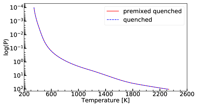
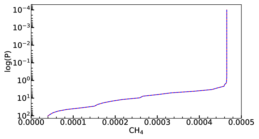
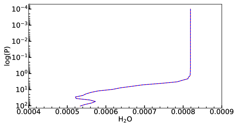
Figure 1: Temperature-pressure (TP) (top panel), CH₄ mixing ratio (middle panel), and H₂O (bottom panel) mixing ratio profiles of a quenched model atmosphere with $T_{\mathrm{eff}}$=1000 K and $\log g$=5.0 calculated by our well-tested premixed code (red, dashed lines) and our new quench-enabled code (blue, solid lines). The relative errors between our premixed models and our new quenched models are $\lesssim 10^{-4}$.

2.2.1 Model spectral resolution and accuracy of the code

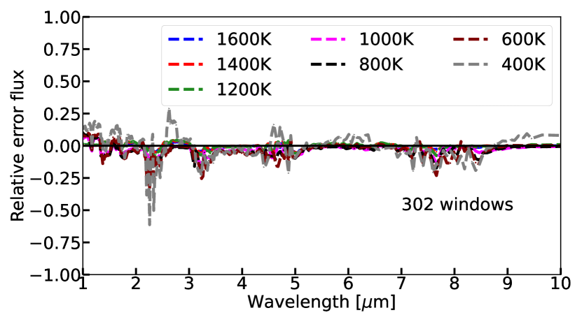
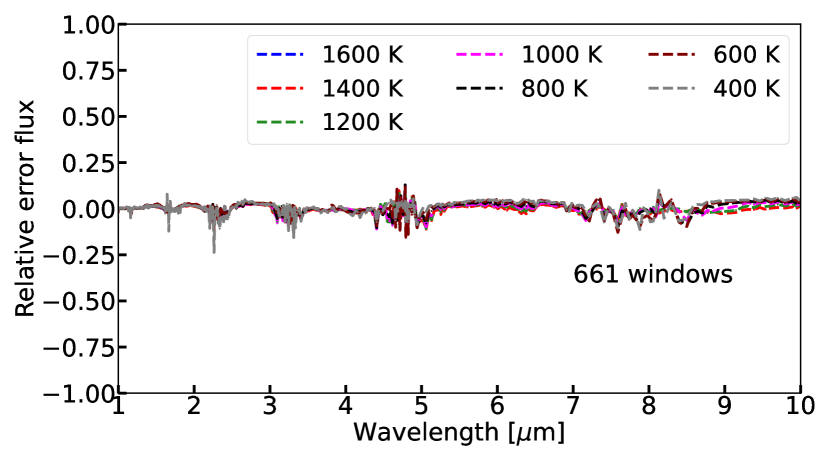
Figure 2: Relative flux error between our well-tested premixed model and our new quenched model for atmospheres. The top panel shows, at a fixed gravity (log $g$=5) $T_{\mathrm{eff}}$ values ranging from 400 K to 1600 K for 302 windows. The bottom panel shows the same as the top panel but for 661 windows. Increasing the number of windows from 302 to 661 windows decreased the average error in our model flux (by 0.001 at 1600 K and a factor of 2 at 400 K).

Amundsen et al. (2017) reported that the spectral resolution of the models could have an effect on the accuracy of the resorting-rebinning of k-coefficients method. Indeed, we found that using our code’s “native” resolution of 196 bins resulted in large discrepancies in the converged TP and composition profiles and spectra of our new code versus those of the well-tested premixed code. Increasing the number of bins progressively improved the accuracy (see Fig. 2). Increasing the number of wavelength bins though, increases the time the model atmosphere code needs to converge to a solution. We ran a number of test cases at different resolutions ranging from 196 to 890 windows and compared the increase in accuracy of the converged TP and composition profiles and spectra with the increase in code running time. Following this procedure we chose to run our grid in a resolution of 661 windows, with the higher density of points typically needed where H₂O and CH₄ opacities were the largest. As can be seen in Fig. 2 the accuracy of comparison to the premixed version depends on the temperature of the model atmosphere, with the colder quenched atmospheres ($\lesssim$ 600 K) showing a larger deviation from the premixed quenched atmospheres (top and middle panels) for the same chemistry.

2.2.2 Validating our code against previously published results

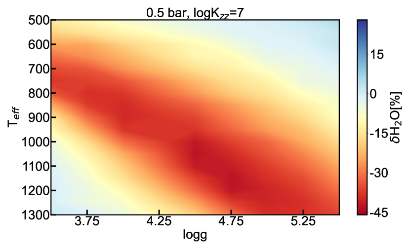
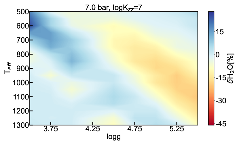
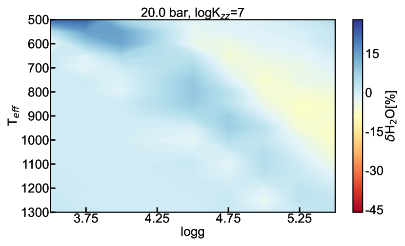
Figure 13: Relative change in H₂O at 0.5 bar (top panel), 7 bar (middle panel) and 20 bar (bottom panel) between a model with $\log K_{zz}$= 7 and the equilibrium chemistry model.

We also compared our output against published results from other groups. In Fig. 3 (top panel) we show spectra between 3 $\mu$m and 16 $\mu$m for our model atmospheres with $T_{\mathrm{eff}}$=900 K, $\log g$=5.5 and for the equilibrium chemistry (black line) and disequilibrium chemistry with $\log K_{zz}$=2 (green line), 4 (red line) and 7 (blue line) cases. For comparison, we also show post-processed disequilibrium spectra (following the same method as in Geballe et al., 2009) for the $\log K_{zz}$= 4 (dark red dashed-dotted line) and 7 (light blue dashed-dotted line) cases. The post-processed spectra are obtained from dis-equilibrium chemistry computed with the TP structure of the atmosphere in equilibrium. The spectra were binned down to a resolution of 200 for plot clarity. The middle panel is a zoom-in in the 3 $\mu$m to 6.5 $\mu$m region, where we overplotted the 900 K, $\log g=5.5$ and $\log K_{zz}=4$ ‘fast’ model of Hubeny & Burrows (2007) (gray, dashed line) from: www.astro.princeton.edu/~burrows/non/non.html. These figures are comparable to Figs.12-13 of Hubeny & Burrows (2007). Finally, the bottom panel shows the volume mixing ratios of our model atmospheres with log $g$=5.5 and $T_{\mathrm{eff}}$=800 K, 1000 K and 1200 K, and for the equilibrium chemistry models (dashed lines) and the disequilibrium chemistry models with $\log K_{zz}=4$ (in [$\mathrm{cm^{2}/s}$]; solid lines). This figure is comparable to Fig. 2 of Hubeny & Burrows (2007).

Our model atmospheres have comparable volume mixing ratio patterns to the model atmospheres of Hubeny & Burrows (2007). However, slight changes in the TP profiles during our iterative calculation of the TP and composition profiles resulted in slightly lower CO content than the equilibrium models even deeper than the CO quenching level, unlike the Hubeny & Burrows (2007) models. The CO absorption in the 4.7 $\mu$m window (middle panel) increased with increasing $\log K_{zz}$ in a comparable way to Hubeny & Burrows (2007).

Comparing the absolute values of our model spectra and composition profiles with the fast model of Hubeny & Burrows (2007) (middle panel of our Fig. 3 and comparison of bottom panel with their Fig. 2), we see that our models have more CO and less CH₄ than the Hubeny & Burrows (2007) fast model, as expected (see also Sect. 4.2 of Zahnle & Marley (2014)). The different opacities used by Hubeny & Burrows (2007) also cause differences in the spectra. Finally, in agreement with these authors, and as first pointed out and explained in (Saumon et al., 2006, end of section 5.3) for Gl 570D, we found that the NH₃ absorption at wavelengths $\gtrsim$10 $\mu$m is relatively insensitive to our $\log K_{zz}$, over the range of values investigated.

Finally, comparing our model disequilibrium spectra with the post-processed disequilibrium spectra we note an overall agreement between 3 $\mu$m and 16 $\mu$m. The most prominent difference is in the $\sim$10.5 $\mu$m NH₃ feature where our absorption is 30% deeper than for the post-processed spectra. In Fig. 4 (bottom panel) we show our disequilibrium model spectrum (blue lines) and the corresponding post-processed spectrum (cyan dashed line) for a $T_{\mathrm{eff}}$=800 K, $\log g$=5.0 model. In this case our $\sim$10.5 $\mu$m NH₃ feature is in agreement with the post-processed model. Both our models are cooler than the equilibrium models (and thus the post-processed models) by 30 K to 120 K throughout the atmosphere. At the pressure range probed by the NH₃ feature the change in temperature and NH₃ content of our atmosphere for the (900 K, 5.5) model is smaller than the change for the (800 K, 5.0) model. This results in a deeper NH₃ feature for our (900 K, 5.5) model, which is closer to the equilibrium feature than the post-processed model. Decoupling the temperature-pressure from the atmospheric chemistry calculation as in the post-processed spectra could thus lead to changes in the spectra for some $T_{\mathrm{eff}}$-$\log g$ combinations and impact our atmospheric characterization.

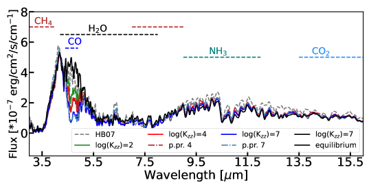
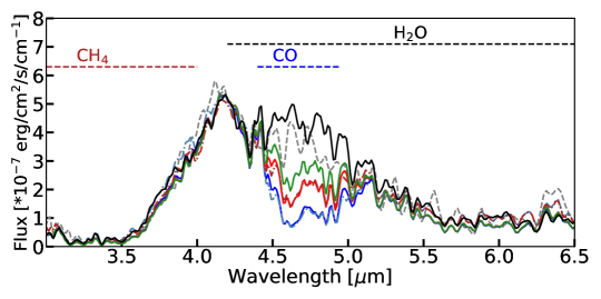
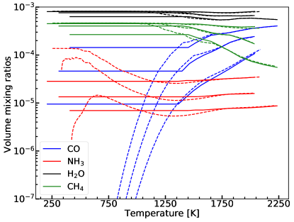
Figure 3: Top panel: 3$\mu$m - 16$\mu$m spectra of our 900 K, log $g$=5.5 model atmospheres with equilibrium chemistry (black line) and with disequilibrium chemistry with $\log K_{zz}$=2 (green line), 4 (red line) and 7 (blue line). We also show the corresponding post-processed disequilibrium spectra for $\log K_{zz}$=4 (dark red dashed-dotted line) and 7 (light blue dashed-dotted line) for reference. The spectra were binned down to a resolution of 200 for plot clarity. Middle panel: Same as middle panel, but zoomed in to wavelengths between 3 and 6$\mu$m. Here, we overplotted the corresponding Hubeny & Burrows (2007) fast model from: www.astro.princeton.edu/$∼$burrows/non/non.html (gray dashed line). Bottom panel: Volume mixing ratios for CH₄(green lines), H₂O (black lines), NH₃ (red lines) and CO (blue lines) for our disequilibrium chemistry models with $\log K_{zz}$=4 (solid lines) and equilibrium chemistry models (dashed lines) for atmospheres with $\log g$=5.5 and $T_{\mathrm{eff}}$=800 K, 1000 K and 1200 K. Note that the colder a model is, the lower its minimum temperature is (so the further to the left the line extends).

2.3 Gliese 570D

Finally, we tested the code against observations of late T-dwarf Gliese 570D. The T7.5 dwarf Gliese 570D (hereafter Gl570D) was observed by Geballe et al. (2001b), Burgasser et al. (2004), Cushing et al. (2006), and Geballe et al. (2009) and was shown to exhibit evidence of disequilibrium chemistry. Gl570D is now considered the archetypal cloud-free brown dwarf atmosphere in disequilibrium. Saumon et al. (2006) fitted the observations of Gl570D and retrieved a temperature of 800-820 K and log $g$=5.09-5.23. Using models of atmospheres with disequilibrium chemistry Saumon et al. (2006) obtained a good fit of the spectrum of Gl570D, including the 10.5$\mu$m NH₃ feature. Saumon et al. (2006) tested different possible sources for the NH₃ depletion in the atmosphere of Gl570D and concluded that it must be due to disequilibrium chemistry. Hubeny & Burrows (2007) also showed that a 800 K, $\log g$=5.0, $\log K_{zz}$=4 model gave a good fit to the 6 $\mu$m - 12 $\mu$m window observations. Line et al. (2015) performed a retrieval on the Gl570D spectra and retrieved a $T_{\mathrm{eff}}$ of 714${}^{+20}_{-23}$K and log $g$=4.76${}^{+0.27}_{-0.28}$.

We fit the spectrum of Gl570D using models at 700 K, 750 K, 800 K and 850 K and log $g$=4.5, 4.75, 5.00 and 5.25. In Fig. 4 we show our model spectra at ($T_{\mathrm{eff}}$, log $g$) = (800 K, 5.0) as representative of the best-fit cases of Saumon et al. (2006) and Hubeny & Burrows (2007). The top panel shows the NIR Gl570D observations dataset (black line), as well as the (800 K, 5.0) equilibrium model (red model) and our $\log K_{zz}$=4 model (blue line), while the bottom panel shows the mid-IR Gl570D observations dataset. We also show a post-processed disequilibrium spectrum for the (800 K, 5.0) model atmosphere with $\log K_{zz}$=4 (cyan, dashed line) for comparison. We binned down our model spectra to a variable resolution comparable to the observations for plot clarity. In agreement with Saumon et al. (2006) and Hubeny & Burrows (2007) our (800 K, 5.0) disequilibrium models gave the best fit to the observations of Gl570D across the 1.1 $\mu$m - 14 $\mu$m spectrum (smaller $\chi^{2}$ by a factor of $\sim$3) with the exception of the 2.0 $\mu$m - 2.2 $\mu$m window, where our disequilibrium models were underluminous in comparison to the observations ($\chi^{2}$ increased by a factor of $\sim$2.2). The (700 K, 5.0) models which are representative of the best-fit case of Line et al. (2015) (not shown here) had a poor fit in the 10.0 $\mu$m - 12 $\mu$m window, where NH₃ dominates, and a worst overall $\chi^{2}$ fit (larger by a factor of 1.8) than the 800 K model. The underluminosity of our models in the K-band and a mismatch for wavelengths shortward of 1.1 $\mu$m is due to inaccuracies in our alkali opacities database and, potentially, our CIA and other opacities in the K-band. Addressing these issues is part of ongoing work. The post-processed spectrum provides a good fit to the observations of Gl570D, and is slightly underluminous in comparison to the observations in the 2.0 $\mu$m - 2.2 $\mu$m window, like our self-consistently calculated spectrum. However, the TP profile of the post-processed spectrum is 15 K to 100 K hotter than our self-consistent TP profile in the pressure range probed by the NIR Gl570D spectrum. This could lead to erroneous conclusions about the atmospheric structure when we characterize an atmosphere with post-processed spectra.

In Fig. 5 we plot the CH₄ and NH₃ volume mixing ratios of our quenched atmosphere models (solid lines) against the corresponding equilibrium ratios (dashed-dotted lines) and the retrieved ratios of Line et al. (2015) (shaded areas) for our best-fit disequilibrium chemistry model at 800 K (top panel) and the 700 K model (bottom panel) that is representative of the best-fit model of Line et al. (2015). For both models the CH₄ content of our model atmospheres was within the range retrieved by Line et al. (2015). For NH₃ however, our best-fit model has a lower volume mixing ratio than what Line et al. (2015) retrieved. The NH₃ volume mixing ratio for the (700 K, 5.0) disequilibrium model was within the range retrieved by Line et al. (2015). We note, however, that the retrieval of Line et al. (2015) took into account only the 1.1-2.3 $\mu$m spectral range, while our best-fit model was also driven by the fit to the strong NH₃ feature in the 10.0-12 $\mu$m window. This suggests that for retrievals in the JWST era the inclusion of the longer wavelength observations will be important to better constrain the NH₃ content of an atmosphere.

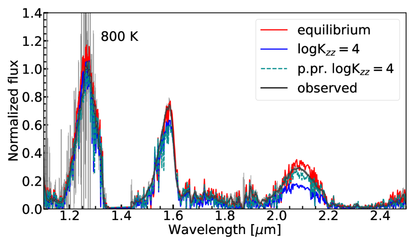
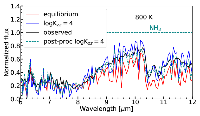
Figure 4: Observed spectrum (black solid line) with error bars (gray lines) of Gl570D and disequilibrium models for an atmosphere with $T_{\mathrm{eff}}$=800 K, $\log g$=5 representative of the best-fit models of Saumon et al. (2006) and Hubeny & Burrows (2007). The models are in equilibrium (red, solid line) or disequilibrium with $\log K_{zz}$= 4 (blue, solid line). We also show a post-processed disequilibrium spectrum with $\log K_{zz}$= 4 (cyan, dashed line) for comparison. Our model spectra were binned down to a variable resolution of 3,000 to 200 comparable to the observations for plot clarity. The error bars are overplotted in both spectra , but the error is too small to be visible in the NH₃ feature.

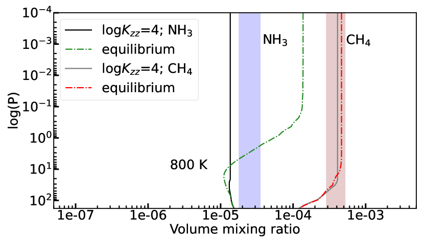
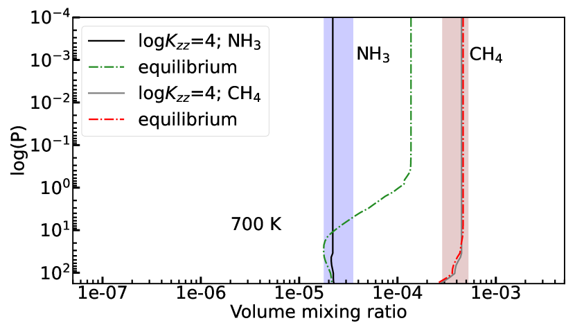
Figure 5: Top panel: Volume mixing ratios of CH₄ and NH₃ for our best-fit model for Gl570D with ($T_{\mathrm{eff}}$, $\log g$) = (800 K, 5.0) (solid lines) against the corresponding equilibrium ratios (dashed-dotted lines) and the retrieved ratios of Line et al. (2015) (shaded areas). Bottom panel: Same as top panel but for the (700 K, 5.0) model, representative of the best-fit model of Line et al. (2015) for Gl570D.

3 Quenched Atmospheres Grid

To examine the effects of quenching on our model atmospheres as a function of temperature ($T_{\mathrm{eff}}$), gravity (log $g$) and eddy diffusion parameter ($K_{zz}$) we have calculated a grid of models from $T_{\mathrm{eff}}$ 500 K to 1300 K (with steps of 50 K), log $g$ ranging from 3.0 to 5.5 (with steps of 0.25; cgs) and log $K_{zz}$=2, 4 and 7 (cgs). For a number of models we also run a case of $\log K_{zz}$=10. Our model atmospheres are cloud–free and have solar metallicity. The extension of the grid to cloudy atmospheres, and atmospheres of different metallicities will be part of future work.

For every model we created an output file for the Sonora grid with the TP and composition profiles for the following species: H₂, He, CH₄, CO, CO₂, NH₃, N₂, H₂O, TiO, VO, FeH, HCN, H, Na, K, PH₃ and H₂S. We then created high resolution emission spectra for these models using the radiative transfer code described in Morley et al. (2015).

In Sect. 3.1 we study the effect of quenching on the TP profiles of the atmospheres, in Sect. 3.2 we study the effect of quenching on the composition profiles and in Sects. 3.3 and 3.4 we study the effect of quenching on the spectra and colors of our model atmospheres.

3.1 TP profiles of quenched atmospheres

In Fig. 6 we show the TP profiles for atmospheres with $\log K_{zz}$=2 (black lines), 4 (purple, dashed lines) and 7 (red, dotted lines) and for the corresponding equilibrium chemistry model atmospheres (green, dashed–dotted lines). The atmospheres have [$T_{\mathrm{eff}}$,log $g$] of [1300 K, 5.00] (top panel), [800 K, 5.00] (middle panel) and [650 K, 5.00] (bottom panel).

Both $\log g$ and $T_{\mathrm{eff}}$ of an atmosphere affect the influence of quenching to the TP profile of the atmosphere. For all models, directly above the quenching level of CH₄-H₂O-CO the atmospheres are colder by $\gtrsim$100 K due to the relative change in the volume mixing ratio of absorbers such as CH₄ and H₂O. At a pressure of $\sim$7 bar the relative change of temperatures were: 18.26% ($\log K_{zz}$=2)–18.4% ($\log K_{zz}$=7) for the [500 K, 5.00] model, 7.9% ($\log K_{zz}$=2)–11.4% ($\log K_{zz}$=7) for the [800 K, 5.00] model, and -2.9% ($\log K_{zz}$=2)–6.3% ($\log K_{zz}$=7) for the [1300 K, 5.00] model. At a pressure of 0.5 bar the corresponding relative changes were: 14.5%–14.6%, 13.9%–16.0% and 10.0%–17.3%.

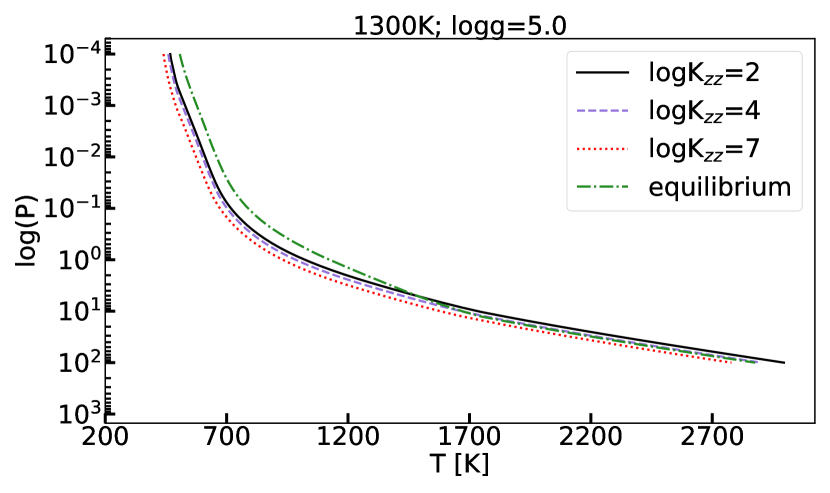
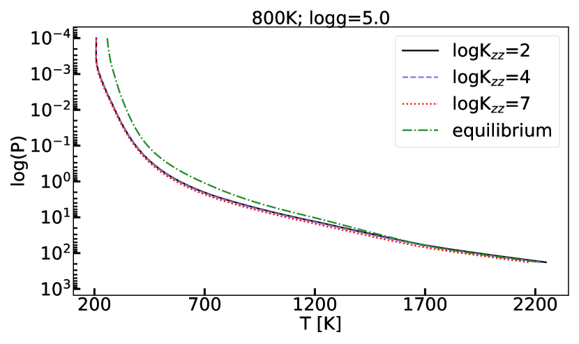
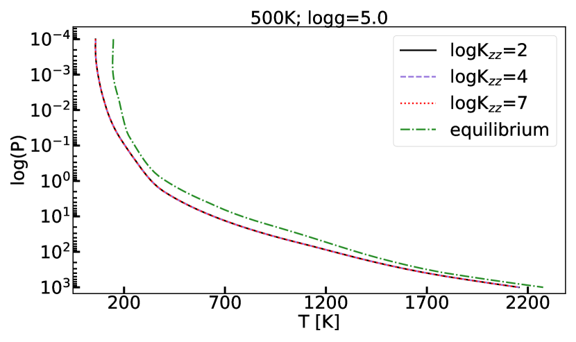
Figure 6: Temperature as a function of pressure for models at [500 K, 5.00] (bottom panel) and for equilibrium chemistry (green, dashed–dotted lines), or disequilibrium with $\log K_{zz}$=2 (black lines), 4 (purple, dashed lines) and 7 (red, dotted lines).

To study further the effect of $\log g$ and $T_{\mathrm{eff}}$ on the TP profile of a model atmosphere, in Fig. 7 we show the TP profiles for atmospheres with $\log g$=5.00, in disequilibrium (solid lines) with $\log K_{zz}$= 4 (top panel) and 7 (bottom panel) and $T_{\mathrm{eff}}$ of 650 K (red lines), 950 K (blue lines) and 1250 K (gray lines) with their corresponding equilibrium profiles (dashed lines); and in Fig. 8 we show the TP profiles for atmospheres with $T_{\mathrm{eff}}$=1000 K, $\log K_{zz}$= 4 (top panel) and 7 (bottom panel) and $\log g$ ranging from 3.0 (green lines) to 5.5 (gray lines).

For a constant gravity $\log g$=5.0 (Fig. 7), the colder a model atmosphere was (i.e., the lower its $T_{\mathrm{eff}}$ was), the colder its upper atmosphere became in reference to the equilibrium model both for $\log K_{zz}$= 4 and 7. For the $\log K_{zz}$= 7 models, the upper atmosphere (P$\lesssim$0.1 bar) cooled by 3.7%-20.9% for the $T_{\mathrm{eff}}$ $\gtrsim$1250 K and by 3.9%-24.8% for the $T_{\mathrm{eff}}$ $\gtrsim$650 K models. The deeper atmosphere cooled down as well, but to a smaller degree. For a constant temperature $T_{\mathrm{eff}}$=1000 K (Fig. 8), the higher the surface gravity of the atmosphere was, the smaller $\delta$T was at all pressures for both $\log K_{zz}$= 4 and 7. This is due to the TP profile of the atmosphere shifting from deeper to lower pressures in the atmosphere and moving nearly vertical to the CO/CH4 equilibrium lines (see Fig.2 of Zahnle & Marley (2014) for a reference CO/CH4 equilibrium line). This affects the opacities of our model atmospheres leading to the observed gravity dependence of $\delta$T.

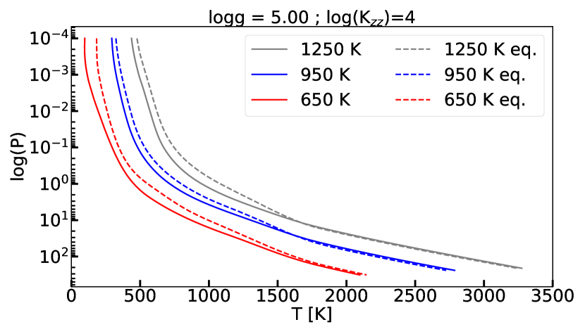
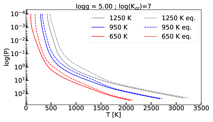
Figure 7: TP profiles for quenched (solid lines) and equilibrium (dashed lines) models for atmospheres with $\log g$=5.0 and $T_{\mathrm{eff}}$ of 1250 K (gray lines), 950 K (blue lines) and 650 K (red lines), and for $\log K_{zz}$= 4 (top panel) and 7 (bottom panel).

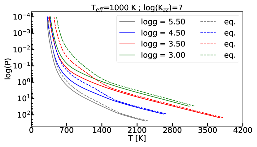
Figure 8: TP profiles for atmospheres with $T_{\mathrm{eff}}$=1000 K and $\log g$=3.0 (green lines), 3.5 (red lines), 4.5 (blue lines) and 5.5 (gray lines) and for $\log K_{zz}$= 4 (top panel) and 7 (bottom panel).

To complete our picture of the effect of $T_{\mathrm{eff}}$ and gravity on $\delta$T in Fig. 9 we show the absolute $\delta$T (=$T_{\mathrm{eq}}-T_{\mathrm{deq}}$) for all our grid models at 0.5 bar (top panels), 7 bar (middle panels) and 20.0 bar (bottom panels), for $\log K_{zz}$=7. The pressures were chosen as representative of the upper, mid and deeper atmosphere. For $\log K_{zz}$= 7 our model atmospheres were cooler than the equilibrium models. For $\log K_{zz}$= 2 (not shown here) our quenched model atmospheres were cooler than the equilibrium chemistry ones across most pressure layers, except at higher $T_{\mathrm{eff}}$ - low g models where at higher pressures the atmospheres heated up.

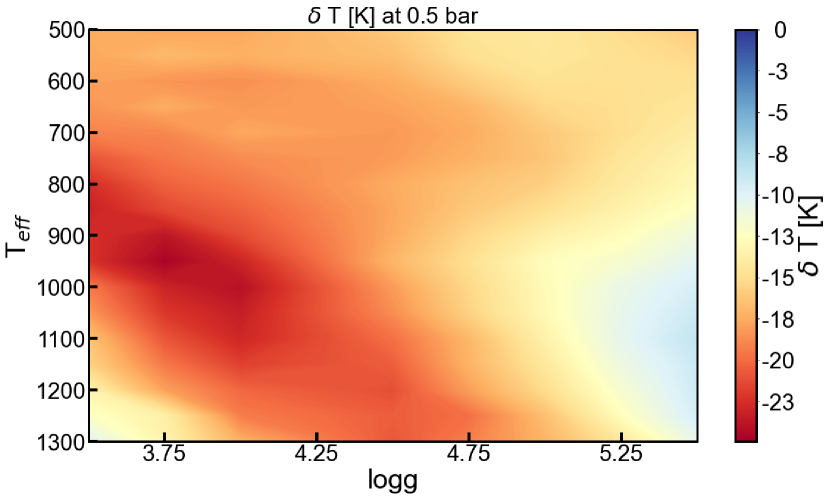
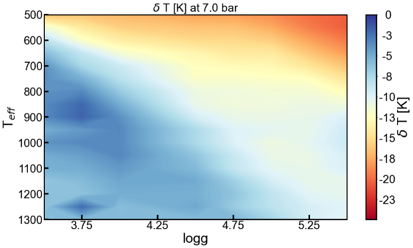
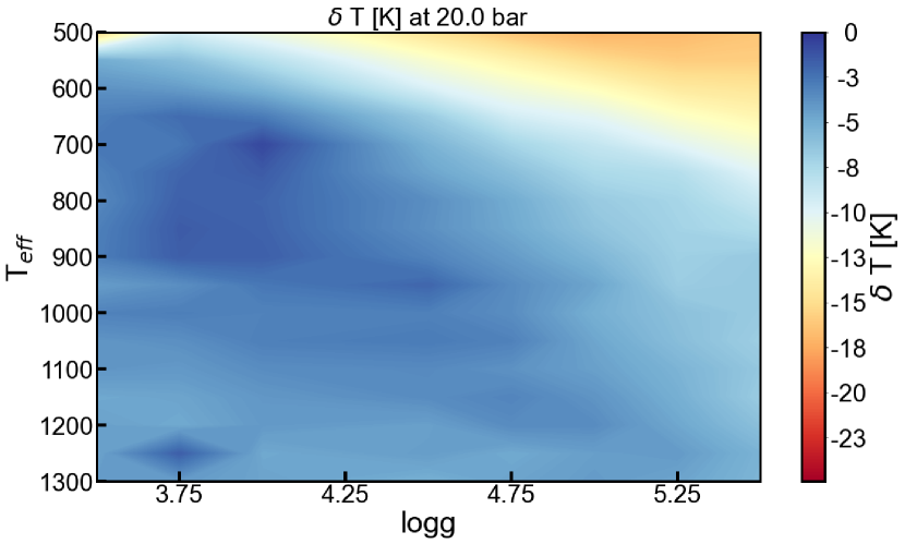
Figure 9: Relative $\delta$T as a function of $\log g$ and $T_{\mathrm{eff}}$ for models with $\log K_{zz}$=7 at 0.5 bar (top panels), 7 bar (middle panels) and 20 bar (bottom panels).

3.2 Composition profiles of quenched atmospheres

In Fig. 10 (top panel) we show the volume mixing ratio profile of H₂O for the quenched and equilibrium model atmospheres for a model atmosphere with $T_{\mathrm{eff}}$ = 800 K, $\log g$=5.0 and $\log K_{zz}$= 2 (black, solid line), 4 (purple, dashed line), 7 (red, dashed–dotted line) and 10 (green, dotted line). We also show (middle panel) the volume mixing ratio of H₂O for model atmospheres with $\log g$=5.0, $\log K_{zz}$= 4 and $T_{\mathrm{eff}}$ of 700 K (red lines), 1000 K (blue lines) and 1300 K (gray lines); and (bottom panel) the volume mixing ratio of H₂O for model atmospheres with $\log K_{zz}$ = 4, $T_{\mathrm{eff}}$ = 1000 K and $\log g$ of 3.0 (green lines), 3.5 (red lines), 4.5 (blue lines) and 5.5 (gray lines).

As expected, with increasing $\log K_{zz}$ our model atmospheres depart further from equilibrium chemistry, with the H₂O volume mixing ratio relatively reduced by 2% for $\log K_{zz}$= 2 to 17% for $\log K_{zz}$= 10. For a constant $\log g$ the departure from equilibrium chemistry depends on the temperature of our model atmospheres (Fig. 10, middle panel). In the upper atmosphere, for $\log K_{zz}$=4 the H₂O volume mixing ratio of our atmosphere was reduced by 2% at 700 K to 38.8% at 1300 K. Finally, as expected (see also Zahnle & Marley, 2014), for a constant temperature the departure from equilibrium chemistry depends strongly on the gravity of our model atmosphere (bottom panel of Fig. 10 and Fig. 11). The smaller $\log g$ is, the larger the depletion of H₂O higher up in the atmosphere is. Due to quenching happening higher up in the atmosphere, the H₂O profile of the atmosphere in deeper layers coincides with the equilibrium chemistry model profile. On the other hand, the larger $\log g$ is the larger the depletion of H₂O deeper in the atmosphere is. As an indication of the changes in the volume mixing ratio of other species with $\log g$ and $\log K_{zz}$, Fig. 11 shows the volume mixing ratio at 0.1 bar for H₂O (blue markers), CH₄ (red markers) and CO (green markers). Our model atmospheres have $T_{\mathrm{eff}}$ = 800 K, $\log g$= 5.0 (squares), 4.25 (circles) and 3.75 (diamonds) and different $\log K_{zz}$ values. The volume mixing ratio of all three species changes with $\log K_{zz}$ for both gravities. Similar to H₂O (bottom panel of Fig. 10), the smaller $\log g$ is, the larger the change in CH₄ and CO is with $\log K_{zz}$. As noted in Zahnle & Marley (2014) $\log g$ affects the $\log K_{zz}$ for which CO dominates the atmosphere.

Finally, Figs. 12 and 13 show the relative changes in the H₂O content of our model atmospheres as a function of $T_{\mathrm{eff}}$ and $\log g$, and for various $\log K_{zz}$ and pressures. These figures are indicative of the trends in the relative change of different species’ volume mixing ratios, and do not intend to show a complete picture of the grid.

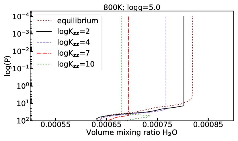
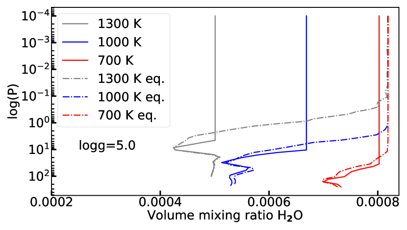
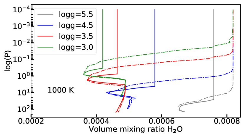
Figure 10: Top panel: Volume mixing ratio of H₂O of our model atmospheres and that of the corresponding equilibrium atmosphere, for atmospheres with $T_{\mathrm{eff}}$ = 800 K, $\log g$=5.0 and $\log K_{zz}$= 2(black, solid line), 4 (red, dashed–dotted line), 7 (red, dashed line) and 10 (green, dotted line). Middle panel: Volume mixing ratio of H₂O for our model atmospheres (solid lines) in comparison to the corresponding equilibrium atmosphere profiles (dashed lines) for atmospheres with $\log g$=5.0, $\log K_{zz}$=4 and $T_{\mathrm{eff}}$ of 1300 K (gray lines), 1000 K (blue lines) and 700 K (red lines). Bottom panel: Volume mixing ratio of H₂O for our model atmospheres (solid lines) in comparison to the corresponding equilibrium atmosphere profiles (dashed lines) for atmospheres with $T_{\mathrm{eff}}$ = 1000 K, $\log K_{zz}$=4 and $\log g$ of 3.0 (green lines),3.5 (red lines), 4.5 (blue lines) and 5.5 (gray lines).

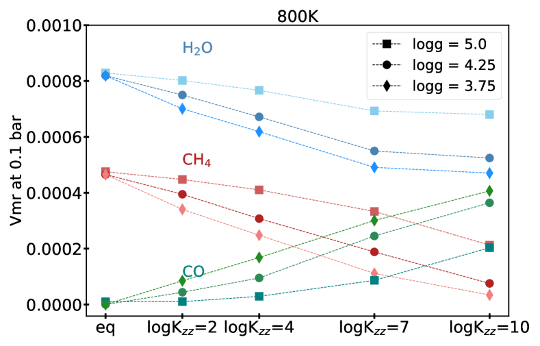
Figure 11: Volume mixing ratio of H₂O (blue), CH₄ (red) and CO (green) at 0.1 bar for different $\log K_{zz}$ values and for a model atmosphere with $T_{\mathrm{eff}}$ = 800 K and $\log g$=5.0 (squares), 4.25 (circles) and 3.75 (diamonds) .

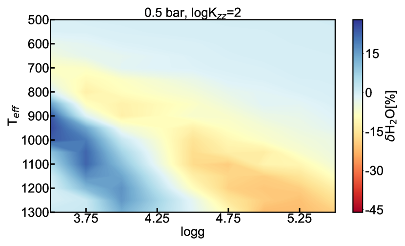
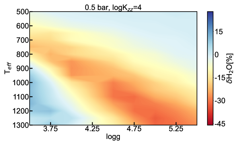
Figure 12: Relative change in H₂O at a pressure of 0.5 bar between a model with $\log K_{zz}$= 2 (top panel) or 4 (bottom panel) and the equilibrium chemistry model, as a function of gravity and effective temperature.

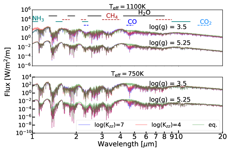
Figure 14: Quenching changes the composition and thus the spectrum of our model atmospheres. Here shown are spectra of a selection of our model atmospheres (top panel 1100 K and bottom panel 750 K) with log $g$=3.5 and 5.25, and log $K_{zz}$=4 (red line) or 7 (blue line) and the corresponding equilibrium model spectrum (green line). The spectra are shifted by an arbitrary amount for plot clarity and downsampled to a resolution of 800. Also shown are some of the major absorption bands for CH₄, CO, H₂O and NH₃, and CO₂.

3.3 Detection of CH4, CO and NH3 in quenched atmospheres

In Fig. 14 we plot spectra of our model atmospheres for $\log g$=3.5 and 5.25, $T_{\mathrm{eff}}$ of 750 K (top two spectra) or 1100 K (bottom two spectra) and $\log K_{zz}$=4 (red line) or 7 (blue line). We also plot the corresponding spectra of model atmospheres with equilibrium chemistry (green line). For plotting clarity we shifted our spectra by arbitrary amounts and binned our spectra down to a resolution of 500.

Quenching of CH₄, CO, H₂O and NH₃ affected the composition profiles of these species in our model atmospheres and thus the detectability of these species in the atmosphere. For $\log g$=5.25 and $T_{\mathrm{eff}}\gtrsim$ 1100 K the changes in the composition of our model atmospheres in reference to the equilibrium model were small for CH₄, H₂O and NH₃ resulting in non-detectable changes in the model spectra in the major absorption bands of these species. Notably, quenching affected the strong CO band around 4.7 $\mu$m resulting in a large difference ($\delta$F$\sim$40%-50% for $\log K_{zz}$=4 or 7 respectively at 1100 K, to $\delta$F$\sim$50%-60% at 750 K) for all atmospheres. In this Section we test the detectability of CH₄, CO, H₂O and NH₃ for our model atmospheres with JWST.

In Fig. 15 (top panel) we plot our model atmosphere spectra for atmospheres with $T_{\mathrm{eff}}$ ranging from 650 K to 1300 K and $\log g$=5.5. Red lines are used for the $\log K_{zz}$=4 models, blue lines for the $\log K_{zz}$=7 models and green lines for the equilibrium chemistry models. The spectra are plotted as they would be observed with JWST using NIRSPEC (covering the 0.97 $\mu$m - 5.14 $\mu$m range). Note that these spectra also cover the wavelength range observed with the NIRISS Single-Object Slitless Spectroscopy (NIRISS SOSS; covering the 0.6 $\mu$m - 2.8 $\mu$m range), but at a higher resolution, so we omit showing the NIRISS SOSS spectra here. We also plot the same models but for $\log g$=4.5 (middle panel) and 3.5 (bottom panel).

For high- and intermediate-gravity atmospheres ($\log g$=5.5 and 4.5) JWST NIRISS-SOSS could detect departures from equilibrium in the H₂O and CH₄ content of an atmosphere for the cooler atmospheres ($\lesssim$600 K), a small change in the NH₃ content might be detectable around $\sim$1.6$\mu$m, but no changes were observable for CO. This is due to the fact that the single CO absorption band in the NIRISS-SOSS wavelength range overlaps with absorption bands of other major species like CH₄ and H₂O. For the low gravities ($\log g$=3.5) JWST NIRISS-SOSS could be able to separate easier the different $\log K_{zz}$ cases in intermediate to cooler atmospheres ($T_{\mathrm{eff}}\lesssim$ 900 K). The inclusion of the 4-5 $\mu$m window with NIRSPec, allowed to detect deviations from equilibrium for the H₂O, CH₄ and possibly NH₃ content of our model atmospheres like NIRISS-SOSS did, but also allowed the detection of variation in the CO content of our model atmospheres around the 4.7 $\mu$m CO-absorption band, especially for the cooler atmospheres ($T_{\mathrm{eff}}\lesssim$ 900 K). Finally, a small change was potentially observable around 4.14 $\mu$m due to changes in the PH₃ content of the colder atmospheres. We note though, that the overlap with a H₂O and a CO absorption band may hinder this detection at low resolutions. The PH₃ feature could be easier detected for higher metallicity objects (Visscher et al., 2006; Miles et al., 2020). Exploring the effect of disequilibrium chemistry on atmospheres with non-solar metallicities will be part of future work.

Finally, we note that the use of MIRI spectroscopy would allow the detectability of NH₃ in disequilibrium through changes in the 10.5$\mu$m NH₃ feature. In particular, our 500 K and 550 K models at a medium resolution (not shown here) showed a decrease in the flux in the 10.5 $\mu$m NH₃ absorption feature by $\sim$40% and $\sim$30% in comparison to the equilibrium flux, allowing the detection of NH₃ in disequilibrium for these cooler model atmospheres.

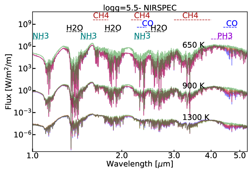
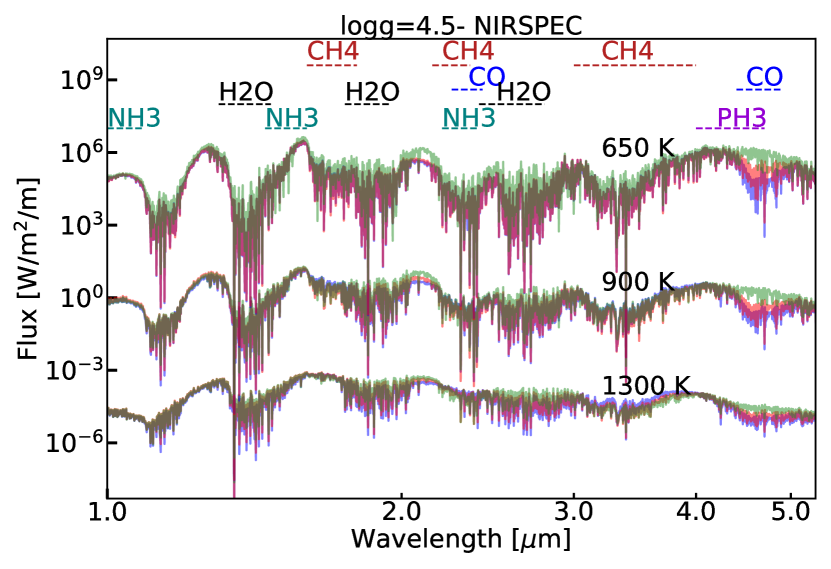
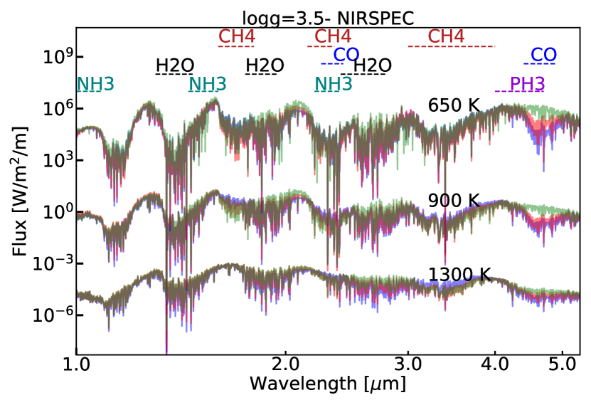
Figure 15: Spectra of a selection of our model atmospheres as they would be observed by JWST with NIRSPEC at high resolution (G140H + G235H + G395H) . Top panel: atmospheres with $\log g$=5.5 and $T_{\mathrm{eff}}$ ranging from 650 K to 1300 K. Green lines are atmospheres with equilibrium chemistry, while red and blue lines are quenched atmospheres with $\log K_{zz}$=4 or 7 respectively. Medium and lower panels: Same as top panel but for $\log g$=4.5 and 3.5 respectively.

3.4 Colors of quenched atmospheres

Quenching changed the composition of our model atmospheres and thus their spectra in comparison to the equilibrium models (see also Sect. 3.3). In this section we study the effect of quenching in the color of our model atmospheres. In particular, we study the effect of quenching on the color that JWST NIRCam would observe for our model atmospheres. We used NIRCam’s F115W filter (J-band), F162M (H), F210M (K) and F356W (L).

In Fig. 16 we show the Color Magnitude Diagram (CMD) for our model atmospheres in J-H (top panel), H-K (upper middle panel) and J-K (bottom panel) for $\mathrm{log}g$ = 3.5 , 4.25 and 5.25. We plot the equilibrium model CMDs (red-orange dots) and our disequilibrium model CMDs for $\log K_{zz}$= 7 (purple-magenta diamonds). Quenching clearly affected the colors of our model atmospheres.

In $H-K$ and $J-K$ all disequilibrium atmospheres are bluer than the equivalent equilibrium chemistry models for all $\log K_{zz}$. In $J-H$ the temperature and gravity of the atmosphere influenced the color change in reference to the equilibrium models. The colder atmospheres ($\lesssim$700 K) turned redder for all models and all $\log K_{zz}$. At intermediate temperatures (700 K$\lesssim T_{\mathrm{eff}}\lesssim$1050 K) atmospheres shifted bluer for $\log K_{zz}=2$ and 4, while they turned redder for $\log K_{zz}=7$. Finally the hotter ($\gtrsim$1100 K) atmospheres turned redder for $\log K_{zz}$= 7, while for $\log K_{zz}$= 2 and 4 they turned bluer, or had approximately the same color as the equilibrium models.

To explain the color differences between our equilibrium and disequilibrium chemistry models we focus on the $\log g$=5.25 models. For the hotter models ($\gtrsim$1,000 K) most pressure layers were depleted in H₂O, CH₄ and NH₃. Some layers appeared to have an overabundance of these species due the disequilibrium atmosphere following a different TP profile than the equilibrium one. For example, at 1300K the disequilibrium model had more H₂O than the equilibrium model deeper in the atmosphere ($\gtrsim$10 bar) and in a narrow pressure layer around $\sim$0.5 and $\sim$2 bar, but it was depleted in H₂O in all other layers. CH₄ was depleted at all pressures $\lesssim$ 1 bar and was overabundant for deeper layers. NH₃ was overabundant at all pressures.

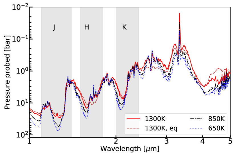
Figure 17: Different bands probe different pressures in an atmosphere. Here shown are the pressures probed at different wavelengths for our $\log K_{zz}$=4 models with $T_{\mathrm{eff}}=$ 1300 K (red line), 850 K (black line) and 650 K (blue line) and $\log g=5.25$. Also shown is the equilibrium 1300 K model (brown, dashed line) for comparison. The J, H and K band passes are also shown for convenience. The abundance profiles of the major absorbents in the pressures probed by the different bands differ between our equilibrium and disequilibrium model atmospheres. These differences lead to different amounts of absorption and thus colors for the disequilibrium and the equilibrium atmospheres.

On average, the J and H band probed the same pressure layers in our 1300 K model atmospheres. The H band (at a high resolution) though, probed a wider range of pressure across the band, varying from $\sim$1 bar at the edges, down to $\sim$15 bar in the center of the band (Fig. 17). The J band on the other hand, probed the $\sim$15-20 bar region throughout the band, with the exception of some narrow lines where lower pressures were probed and the wings of the band where pressures around $\sim$3.5 bar were probed. The pressures probed by both J and H bands were depleted in H₂O, had slightly overabundant NH₃, while CH₄ was slightly overabundant for J and depleted in pressures probed by the H band. This resulted in the J band being dimmer for the disequilibrium model than the equilibrium one ($\delta F\sim$14%), while the H band had comparable brightness for the disequilibrium and equilibrium models. This resulted in redder J-H colors for the disequilibrium model.

The disequilibrium model K band got dimmer than the equilibrium model K band ($\delta F\sim$33%), resulting in overall bluer J-K colors than the equilibrium chemistry models. The reason for the dimmer K band was that its longer wavelengths are dominated by a CH₄ and a NH₃ band, and its shorter ones by an H₂O band. The K band probed pressures between $\sim$0.5 and $\sim$4.5 bar were NH₃ was overabundant by $\sim$50%-150% (relative variation). In these pressures H₂O was slightly overabundant as well, while CH₄ was slightly underabundant. This resulted in a dimmer K-band for $\lambda\lesssim$ 2.15 $\mu$m. The longer wavelength part of the K band was slightly dimmer or comparable to the equilibrium model one, due to including an NH₃ and a CH₄ window. Finally, errors in our CIA opacity database could also affect our K band and result in further dimming as for Gl570D (see Sect. 2.3). Overall this resulted in a dimmer K-band (relative change of $\sim$34% vs $\sim$13% for the J-band for the $\log K_{zz}$= 7 model) and bluer J-K and H-K colors.

For intermediate models at $\sim$900 K and $\log g$=5.25, H₂O and CH₄ were depleted for most pressures except the deeper atmosphere (deeper than $\sim$10bar for $\log K_{zz}$= 4 to $\sim$30bar for $\log K_{zz}$= 7). Finally NH₃ was depleted for all pressures $\lesssim$ 10 bar. The pressure ranges probed by the J, H and K bands in our 900K model differ from those at 1300K. The J band for the 900K model probed pressures around 50 bar (see Fig. 17), which resulted in the J band being dimmer for the disequilibrium than the equilibrium models (relative $\delta F\lesssim$18%), since the pressure range probed covers areas where H₂O is overabundant by a few percent ($\sim$4%; all percentages are relative variations). The H band probed pressures around 15 bar. In the pressures probed by the H band, CH₄ was depleted by $\sim$20-30% and NH₃ was overabundant by $\sim$10%-30% (for $\log K_{zz}$= 4 and 7), which resulted in an overall dimmer H band (average relative $\delta F\sim$ 20%) and a slightly bluer J-H color for our disequilibrium atmosphere than the equilibrium atmosphere. Finally, the K band of our disequilibrium model became dimmer than the equilibrium one (average relative $\delta F\sim$ 46%) due to an overabundance of NH₃ and CH₄ in the pressures probed by the band. This resulted in bluer J-K colors for the disequilibrium atmospheres.

Finally, for the even colder models at $\sim$650 K, the pressures probed by the J, H and K bands are $\gtrsim$25 bar, which are overabundant in CH₄, NH₃ and H₂O, resulting in a dimmer J band (relative $\delta F\sim$ 48%), a less dim H band (relative $\delta F\sim$ 35%) and a dimmer K band (relative $\delta F\sim$ 81%) resulting in redder J-H colors and bluer J-K and H-K colors.

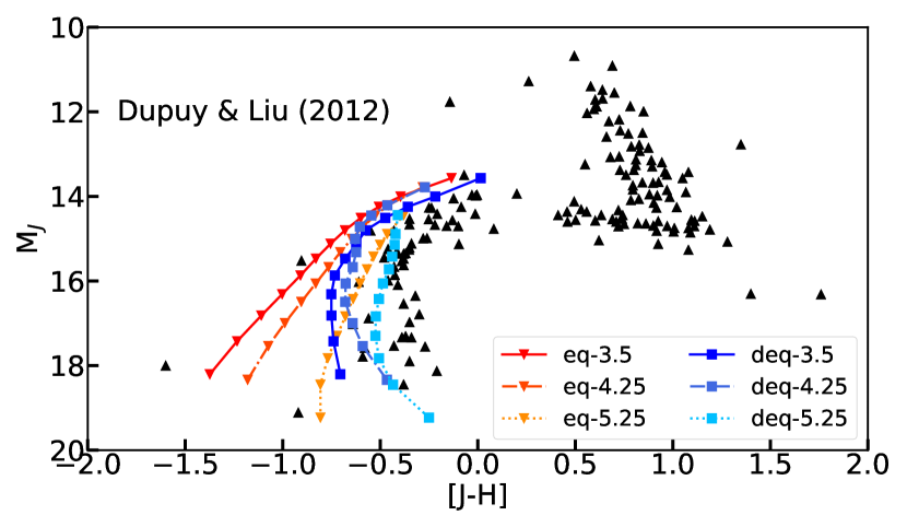
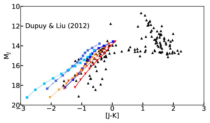
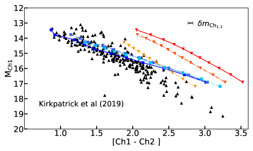
Figure 18: CMDs of our equilibrium and disequilibrium atmospheres with $\log K_{zz}$=7, and the MKO observations of Dupuy & Liu (2012) (top and middle panel) and Spitzer data from Kirkpatrick et al. (2019) (bottom panel) . Color and line coding are similar to Fig. 16. Note that for this plot we used the MKO (top and middle panel) and Spitzer IRAC filters (bottom panel) on our model spectra, to match the observations. For the IRAC data we also plot the average error bar ($\delta m$) in the photometry for reference.

In Fig. 18 we plot our M_J vs J-H and J-K CMD against the observations of Dupuy & Liu (2012) (top and middle panel), and the Spitzer IRAC M_Ch1 vs Ch1-Ch2 against the ensemble of T and Y dwarfs presented in Kirkpatrick et al. (2019). Note that for this plot we used the MKO and Spitzer IRAC filters on our model spectra, to match the data from Dupuy & Liu (2012) and Kirkpatrick et al. (2019). We also note that we don’t intend this plot as a characterization effort for any of the Dupuy & Liu (2012) or the Kirkpatrick et al. (2019) targets since both our disequilibrium and equilibrium models are cloud-free, solar metallicity models while a number of these targets are expected to be (at least partially) cloudy and could potentially have non-solar metallicities. Finally, to keep our plot consistent with the data we only plot models with $T_{\mathrm{eff}}\lesssim$ 1000 K for the Spitzer IRAC dataset.

The disequilibrium chemistry models turned the J-H colors of our atmospheres redder than the equilibrium chemistry models for the later T-type atmospheres. This is in agreement with observations. However, comparing our models with the Dupuy & Liu (2012) observations in the T-dwarf regime it can be seen that our models are still bluer than the data for intermediate and low gravities (3.5 and 4.25 here). All our model atmospheres are cloud-free. The introduction of clouds and hazes in an atmosphere is known to turn the colors of atmospheres redder (Morley et al., 2012). The color discrepancy between our model atmospheres and observations necessitates extending the disequilibrium chemistry model grid to cloudy atmospheres. This will be part of a future paper. Based on their J-H and H-K (not shown here) colors a number of the observed early T dwarfs reside in both the equilibrium and disequilibrium chemistry space. When J-H, J-K and H-K is taken into account, our disequilibrium chemistry models fit better the mid T and later dwarfs than the equilibrium models. Additionally, the disequilibrium chemistry models give a better fit to the Spitzer 3.6 $\mu$m and 4.5 $\mu$m (Ch1 and Ch12; bottom panel of Fig. 18) for most of the ensemble of T dwarfs presented in Kirkpatrick et al. (2019). For the latest T ($\gtrsim$T8.5) and Y dwarfs disequilibrium chemistry alone cannot provide a good match to the observed Spitzer colors. However, clouds are expected to play a crucial role in these atmospheres (Morley et al., 2012) and affect their colors. In a future paper we will extend the disequilibrium chemistry model grid to cloudy atmospheres and revisit this plot.

Our findings support the importance of disequilibrium chemistry for T type dwarfs, which was already suggested by Saumon et al. (2006, 2007) based on observations of Gl570D, 2MASSJ04151954-0935066 and 2MASSJ12171110-0311131. A number of the T dwarfs in our sample like 2MASSJ11145133-2618235 (Leggett et al., 2007a), ULASJ141623.94+134836.3 (Burgasser et al., 2010), 2MASSJ09393548-2448279 (Burgasser et al., 2008) and 2MASSJ12373919+6526148 (Liebert & Burgasser, 2007) have already been suggested to be in disequilibrium. For example, Burgasser et al. (2008) showed that the spectrum of 2M0939 (T8) was best fit with a $\log K_{zz}$=4 model. ULAS J1416+1348 (T7.5) was also found to be best-fit by a $\log K_{zz}$=4 model by Burgasser et al. (2010). On the other hand, 2M1237 (T7) and 2M1114 (T7.5) were observed to have faint K-bands which Liebert & Burgasser (2007) and Leggett et al. (2007a) attributed to a subsolar metallicity ([m/H]$\sim$-0.3 for 2M1114) or high gravity. These authors did not explore the possibility of disequilibrium chemistry for these targets. Long wavelength coverage spectra that help retrieve the abundances of multiple species would allow us to disentangle the effect of metallicity and disequilibrium chemistry for these targets.

4 Discussion and Conclusions

JWST will enable the imaged exoplanet and brown dwarf community to study in more detail a range of exoplanet and brown dwarf atmospheres and perform comparative studies of their properties as a function of atmospheric properties ($T_{\mathrm{eff}}$, $\log g$, metallicity etc). The long-wavelength-coverage, high quality spectra of exoplanet and brown dwarf atmospheres that JWST will acquire will allow us to probe simultaneously a wider range of pressures than ever before and constrain chemistry and cloud changes in atmospheres as a function of pressure. JWST will also provide us with time-resolved observations of imaged exoplanets and cooler brown dwarfs of comparable quality to what HST does for L/T transition brown dwarfs today(Kostov & Apai, 2013). This will allow us to constrain the time-variability of chemistry and clouds in these atmospheres. However, to do that accurately we will need models that properly account for vertical mixing in the atmosphere.

The departure of an atmosphere from equilibrium chemistry, i.e., how strong its vertical mixing is, depends on the atmosphere’s properties and the eddy diffusion coefficient ($\log K_{zz}$ in this paper) of an atmosphere. The latter is also an important parameter for constraining the cloud formation in the atmosphere (e.g., Marley et al., 2013), thus observational constrains of $\log K_{zz}$ are of high importance to the community. Recently, e.g., Miles et al. (2020) presented low resolution ground-based observations of seven late T to Y brown dwarfs and compared their observations against models of atmospheres with disequilibrium chemistry to constrain the $\log K_{zz}$ of these atmospheres. Miles et al. (2020) showed that $\log K_{zz}$ spans a range of values in these atmospheres from 4 to 8.5, and discussed how comparing these values against the maximum $\log K_{zz}$ predicted from theory can help constrain the existence of detached convective zones in warmer atmospheres. In the coming decade JWST will allow for the first time to constrain changes in $\log K_{zz}$ as a function of pressure in atmospheres and potential trends with atmospheric properties such as $T_{\mathrm{eff}}$ and $\log g$. Such observations will allow us to constrain in unprecedented detail the vertical structure of atmospheres, including the potential existence of detached convective zones predicted by theory (see, e.g., Marley & Robinson, 2015). The accuracy of our results though, will depend on the accuracy of our models. For this reason sets of models that use a self-consistent scheme to study the effect of quenching on atmospheres are necessary for the JWST era.

In this paper we presented an extension of the atmospheric structure code of M. S. Marley and collaborators (e.g., Marley et al. 2021 to calculate the TP and composition profiles of atmospheres in disequilibrium, in a self-consistent way (see Sect.2). We validated the new code against its well tested equilibrium chemistry version, as well as previously published results (Sect. 2.2), and tested the fit of our new non-equilibrium models against observations of Gl570D (Sect. 2.3), which is considered the archetypal cloud-free brown dwarf atmosphere with signs of disequilibrium chemistry. A number of differences between our models and the observed spectra were noted that are related to inaccuracies in our alkali opacity database for wavelengths shortward of 1.1 $\mu$m and, potentially, our CIA opacity in the K-band. Addressing these issues is part of ongoing work.

The extension of our code presented here, opens up the possibility to model more complex atmospheres with variable $\log K_{zz}$ profiles in the future. Flasar & Gierasch (1978) and later Wang et al. (2014), e.g., predicted that Jupiter and Saturn will show latitudinal variation of $\log K_{zz}$ due to the planet’s rotation. Wang et al. (2014), e.g., showed that the $\log K_{zz}(P)$ profiles in Jupiter should change with latitude, with the value of $\log K_{zz}$ changing by more than an order of magnitude for a given temperature layer between $0^{\circ}$ and $80^{\circ}$ latitude. The changes in Saturn were about two orders of magnitude. Similar variable profiles with pressure and latitude could exist in imaged atmospheres and they would affect the chemical profiles and cloud formation in these atmospheres. Additionally, the existence of detached convective zones in some atmospheres would locally change the $\log K_{zz}$ profile, making the use of a simple $\log K_{zz}$ profile as used in this paper inaccurate for the characterization of the three-dimensional structure of these atmospheres. Thus, updated models with variable $\log K_{zz}$ may be needed in the future.

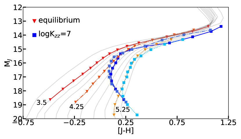
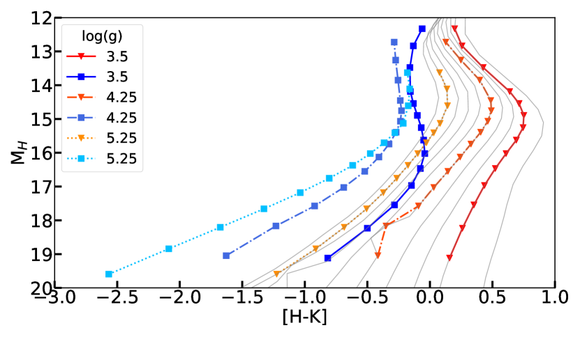
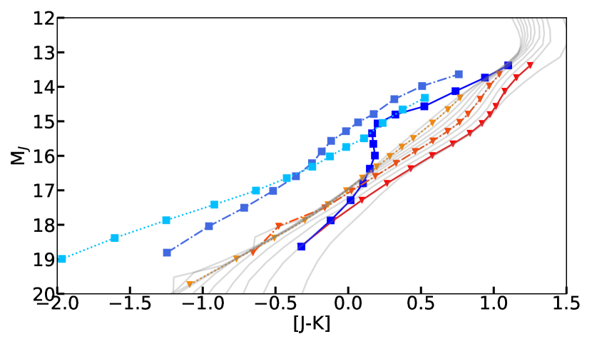
Figure 16: Color Magnitude Diagrams (CMDs) for three gravities ($\log g=3.5$ (solid lines), 4.25 (dashed-dotted lines) and 5.25 (dotted lines)) of our equilibrium atmospheres (red-orange triangles) and disequilibrium atmospheres with $\log K_{zz}$=7 (blue squares). Radii computed from our equilibrium model evolution (Marley et al. 2021). Our model atmospheres range from 500K to 1000K with a step of 50K, and 1000K to 1300K with a step of 100K. Our $J$, $H$ and $K$ correspond to JWST F115W, F162M, and F210M respectively. Overplotted with gray lines are the equilibrium tracks from the Sonora Bobcat models Marley et al. (2021). The gravities of the overplotted Bobcat models range from $\log g=3.0$ to $5.5$ with a step of 0.25.

In the JWST era the Direct Imaging community will have access to high resolution observations of imaged atmospheres in the near and mid infrared. In Sect. 3.3 we showed that using NIRISS and NIRSpec observations we should be able to distinguish between (at least the cloud-free) cooler atmospheres with disequilibrium or equilibrium chemistry. In particular, both NIRISS and NIRSpec should allow the detection of disequilibrium in H₂O, CH₄ and NH₃, while the longer wavelength observations of NIRSpec should also allow the detection of CO in disequilibrium. In Sect. 2.3 when we compared our best-fit model volume mixing ratio of NH₃ against the retrieved ratio of Line et al. (2015), we showed that omitting the 10 $\mu$m -12 $\mu$m observations could have affected their best-fit model. This suggests that in the JWST era MIRI MRS observations will also be important for accurate NH₃ retrievals.

NH₃ has been detected in disequilibrium in some cooler T dwarfs (Canty et al., 2015) and Y dwarfs (Cushing et al., 2011). Overall our coolest disequilibrium model at 500 K, for $\log g$= 5.0 was depleted in NH₃ (relative difference of -50%) as expected. This was detectable in the major NH₃ feature around 10.5 $\mu$m, which showed a lack of NH₃ in the quenched model atmosphere. However, in the deeper pressures probed in the 1.0-1.3 $\mu$m and 1.5-1.6 $\mu$m windows, which include NH₃ absorption windows, the cooling in the TP profile of our atmosphere (at those pressures) resulted in an overabundance of NH₃ which should be detectable for some atmospheres. We are currently extending our grid to cooler atmospheres (down to 200 K), in the realm of Y-dwarfs, where Cushing et al. (2011) reported a possible detection of NH₃ in the atmosphere of WISEP-J1738 (350 K - 400 K) in the 1.5-1.6 $\mu$m window. Fig. 19 shows an example of how NH₃ excess in our cooler atmospheres changed the H-band in a comparable way to the tentative detection on WISEP J1738+2732 by Cushing et al., 2011.

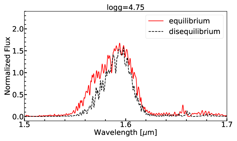
Figure 19: Normalized H-band for model atmospheres with $\log g$=4.75 at 350K. Solid line is an atmospheres with equilibrium chemistry and dashed line with $\log K_{zz}$=7. The models are binned down to a resolution of 1800 for plot clarity. The model in disequilibrium shows a comparable NH₃ enhancement to the tentative detection on WISEP J1738+2732 (Cushing et al., 2011).

A similar dependence on gravity appeared in our detection of CO, with the lower gravity models showing detectable disequilibrium CO absorption around 4.7 $\mu$m for the cooler atmospheres. Finally, for most of our model atmospheres the detection of CH₄ is easier at higher gravities than at lower gravities, (see Fig. 15) in agreement with observations that suggest that low gravity planetary mass objects are depleted in CH₄ in comparison to their brown dwarf analogues (that have a higher surface gravity).

In this paper we showed that, at least for cloud-free atmospheres, disequilibrium chemistry results in redder J-H colors for our model atmospheres (Sect. 3.4). For smaller values of $\log K_{zz}$ only the cooler quenched atmospheres ($\lesssim$ 700 K) turned red at all gravities. At $\log K_{zz}$ = 7 disequilibrium chemistry resulted in redder colors even for atmospheres as hot as 1200 K (Fig. 16 and Sect. 3.4). A number of brown dwarfs and planetary mass objects have been detected that are redder in J-H than their standard field counterparts, like WISEP J004701.06+680352.1 (W0047; Gizis et al., 2012), 2MASS J12073346-3932539, the planets of the HR8799 system (2M1207b Oppenheimer et al., 2013; Currie et al., 2011; Skemer et al., 2014) and others. Most of these atmospheres are expected to be cloudy. For example, both W0047 and 2M1207b show rotational variability which is related to cloud patchiness (Lew et al., 2016; Zhou et al., 2016), and planetary mass companion observations are best fit by cloudy models (e.g., Skemer et al., 2014). Clouds will affect the colors of the atmosphere, but a number of these atmospheres are also CH₄ depleted (Biller & Bonnefoy, 2018) hinting to disequilibrium chemistry in their atmospheres (see, e.g., Barman et al., 2015). Our cloud-free model atmospheres at the temperatures and gravities that are representative of the planets of the HR8799 system (900 K- 1100 K and $\log g$ $\lesssim$4) and for $\log K_{zz}$ = 7 (Barman et al., 2015) became redder in J-H with $\delta$[J-H] = 0.12 to 0.26. Observations of the HR8799 system planets found a color difference from field brown dwarfs that is comparable or larger than what our cloud-free atmospheres showed. Clouds and disequilibrium chemistry are expected to interplay in the atmosphere and affect its color. Clouds are expected to turn atmospheres redder and deplete some of the available chemical species changing the mixing ratio of species in the atmosphere. This hints to the importance of extending the Sonora grid to cloudy atmospheres with disequilibrium chemistry, which will be part of future work.

Finally, we compared the Color Magnitude Diagrams (CMD) of our disequilibrium and equilibrium models against MKO observations of brown dwarfs by Dupuy & Liu (2012) and Spitzer data from Kirkpatrick et al. (2019) (Sect. 3.4). We noted that our disequilibrium chemistry models give a better fit to photometry of mid to late T type brown dwarfs, supporting the importance of disequilibrium chemistry for T type dwarfs (Saumon et al., 2006, 2007). In particular, only disequilibrium models could fit the Spitzer colors of Kirkpatrick et al. (2019). The equilibrium models have more CH₄ and less CO than the observed atmospheres so they appear redder than the latter. On the other hand, disequilibrium chemistry increases the CO content of the atmosphere and reduces its CH₄ content (Fig. 15), which results to bluer colors in agreement with the observations. A number of these target atmospheres have already been suggested to be in disequilibrium. Previous fitting of spectra for some of these targets suggested that a subsolar metallicity or high gravity, may be responsible for their different colors, but the authors did not explore the possibility of disequilibrium chemistry for these targets. Refitting these observations with equilibrium and disequilibrium chemistry models at different metallicities would be of interest. Extending the Sonora grid to atmospheres of different metallicities with disequilibrium chemistry will be part of future work.

Following the Sonora bobcat models, our models will be archived in Zenodo under https://zenodo.org/record/4450269.

Acknowledgements. TK acknowledges the University of Central Florida Advanced Research Computing Center high-performance computing resources made available for conducting the research reported in this paper (https://arcc.ist.ucf.edu). Part of this work was performed under the auspices of the U.S. Department of Energy under Contract No. 89233218CNA000001. JJF, MSM, CVM, RL, and RSF acknowledge the support of NASA Exoplanets Research Program grant 80NSSC19K0446.

References

- Allard (2014) Allard, F. 2014, in IAU Symposium, Vol. 299, Exploring the Formation and Evolution of Planetary Systems, ed. M. Booth, B. C. Matthews, & J. R. Graham, 271–272
- Allard et al. (2012) Allard, F., Homeier, D., & Freytag, B. 2012, Philosophical Transactions of the Royal Society of London Series A, 370, 2765
- Amundsen et al. (2017) Amundsen, D. S., Tremblin, P., Manners, J., Baraffe, I., & Mayne, N. J. 2017, A&A, 598, A97
- Barman et al. (2015) Barman, T. S., Konopacky, Q. M., Macintosh, B., & Marois, C. 2015, ApJ, 804, 61
- Biller & Bonnefoy (2018) Biller, B. A. & Bonnefoy, M. Exoplanet Atmosphere Measurements from Direct Imaging, 101
- Buenzli et al. (2015) Buenzli, E., Saumon, D., Marley, M. S., Apai, D., Radigan, J., Bedin, L. R., Reid, I. N., & Morley, C. V. 2015, ApJ, 798, 127
- Burgasser et al. (2010) Burgasser, A. J., Cruz, K. L., Cushing, M., Gelino, C. R., Looper, D. L., Faherty, J. K., Kirkpatrick, J. D., & Reid, I. N. 2010, ApJ, 710, 1142
- Burgasser et al. (2006) Burgasser, A. J., Geballe, T. R., Leggett, S. K., Kirkpatrick, J. D., & Golimowski, D. A. 2006, ApJ, 637, 1067
- Burgasser et al. (2004) Burgasser, A. J., McElwain, M. W., Kirkpatrick, J. D., Cruz, K. L., Tinney, C. G., & Reid, I. N. 2004, AJ, 127, 2856
- Burgasser et al. (2008) Burgasser, A. J., Tinney, C. G., Cushing, M. C., Saumon, D., Marley, M. S., Bennett, C. S., & Kirkpatrick, J. D. 2008, ApJ, 689, L53
- Burningham et al. (2011) Burningham, B., Leggett, S. K., Homeier, D., Saumon, D., Lucas, P. W., Pinfield, D. J., Tinney, C. G., Allard, F., Marley, M. S., Jones, H. R. A., Murray, D. N., Ishii, M., Day-Jones, A., Gomes, J., & Zhang, Z. H. 2011, MNRAS, 414, 3590
- Burningham et al. (2017) Burningham, B., Marley, M. S., Line, M. R., Lupu, R., Visscher, C., Morley, C. V., Saumon, D., & Freedman, R. 2017, MNRAS, 470, 1177
- Canty et al. (2015) Canty, J. I., Lucas, P. W., Yurchenko, S. N., Tennyson, J., Leggett, S. K., Tinney, C. G., Jones, H. R. A., Burningham, B., Pinfield, D. J., & Smart, R. L. 2015, MNRAS, 450, 454
- Currie et al. (2011) Currie, T., Burrows, A., Itoh, Y., Matsumura, S., Fukagawa, M., Apai, D., Madhusudhan, N., Hinz, P. M., Rodigas, T. J., Kasper, M., Pyo, T.-S., & Ogino, S. 2011, ApJ, 729, 128
- Cushing et al. (2011) Cushing, M. C., Kirkpatrick, J. D., Gelino, C. R., Griffith, R. L., Skrutskie, M. F., Mainzer, A., Marsh, K. A., Beichman, C. A., Burgasser, A. J., Prato, L. A., Simcoe, R. A., Marley, M. S., Saumon, D., Freedman, R. S., Eisenhardt, P. R., & Wright, E. L. 2011, ApJ, 743, 50
- Cushing et al. (2006) Cushing, M. C., Roellig, T. L., Marley, M. S., Saumon, D., Leggett, S. K., Kirkpatrick, J. D., Wilson, J. C., Sloan, G. C., Mainzer, A. K., Van Cleve, J. E., & Houck, J. R. 2006, ApJ, 648, 614
- Drummond et al. (2016) Drummond, B., Tremblin, P., Baraffe, I., Amundsen, D. S., Mayne, N. J., Venot, O., & Goyal, J. 2016, A&A, 594, A69
- Dupuy & Liu (2012) Dupuy, T. J. & Liu, M. C. 2012, ApJS, 201, 19
- Fegley & Lodders (1996) Fegley, Bruce, J. & Lodders, K. 1996, ApJ, 472, L37
- Flasar & Gierasch (1978) Flasar, F. M. & Gierasch, P. J. 1978, Geophysical and Astrophysical Fluid Dynamics, 10, 175
- Fortney et al. (2008) Fortney, J. J., Lodders, K., Marley, M. S., & Freedman, R. S. 2008, ApJ, 678, 1419
- Fortney et al. (2005) Fortney, J. J., Marley, M. S., Lodders, K., Saumon, D., & Freedman, R. 2005, ApJL, 627, L69
- Geballe et al. (2009) Geballe, T. R., Saumon, D., Golimowski, D. A., Leggett, S. K., Marley, M. S., & Noll, K. S. 2009, ApJ, 695, 844
- Geballe et al. (2001a) Geballe, T. R., Saumon, D., Leggett, S. K., Knapp, G. R., Marley, M. S., & Lodders, K. 2001a, ApJ, 556, 373
- Geballe et al. (2001b) —. 2001b, ApJ, 556, 373
- Gizis et al. (2012) Gizis, J. E., Faherty, J. K., Liu, M. C., Castro, P. J., Shaw, J. D., Vrba, F. J., Harris, H. C., Aller, K. M., & Deacon, N. R. 2012, AJ, 144, 94
- Goody et al. (1989) Goody, R., West, R., Chen, L., & Crisp, D. 1989, J. Quant. Spec. Radiat. Transf., 42, 539
- Hubeny & Burrows (2007) Hubeny, I. & Burrows, A. 2007, ApJ, 669, 1248
- Kirkpatrick et al. (2019) Kirkpatrick, J. D., Martin, E. C., Smart, R. L., Cayago, A. J., Beichman, C. A., Marocco, F., Gelino, C. R., Faherty, J. K., Cushing, M. C., Schneider, A. C., Mace, G. N., Tinney, C. G., Wright, E. L., Lowrance, P. J., Ingalls, J. G., Vrba, F. J., Munn, J. A., Dahm, S. E., & McLean, I. S. 2019, ApJS, 240, 19
- Kitzmann et al. (2019) Kitzmann, D., Heng, K., Oreshenko, M., Grimm, S. L., Apai, D., Bowler, B. P., Burgasser, A. J., & Marley, M. S. 2019, arXiv e-prints, arXiv:1910.01070
- Kostov & Apai (2013) Kostov, V. & Apai, D. 2013, ApJ, 762, 47
- Kreidberg et al. (2014) Kreidberg, L., Bean, J. L., Désert, J.-M., Benneke, B., Deming, D., Stevenson, K. B., Seager, S., Berta-Thompson, Z., Seifahrt, A., & Homeier, D. 2014, Nature, 505, 69
- Leggett et al. (2007a) Leggett, S. K., Marley, M. S., Freedman, R., Saumon, D., Liu, M. C., Geballe, T. R., Golimowski, D. A., & Stephens, D. C. 2007a, ApJ, 667, 537
- Leggett et al. (2007b) Leggett, S. K., Saumon, D., Marley, M. S., Geballe, T. R., Golimowski, D. A., Stephens, D., & Fan, X. 2007b, ApJ, 655, 1079
- Lew et al. (2016) Lew, B. W. P., Apai, D., Zhou, Y., Schneider, G., Burgasser, A. J., Karalidi, T., Yang, H., Marley, M. S., Cowan, N. B., Bedin, L. R., Metchev, S. A., Radigan, J., & Lowrance, P. J. 2016, ApJL, 829, L32
- Liebert & Burgasser (2007) Liebert, J. & Burgasser, A. J. 2007, ApJ, 655, 522
- Line et al. (2015) Line, M. R., Teske, J., Burningham, B., Fortney, J. J., & Marley, M. S. 2015, ApJ, 807, 183
- Madhusudhan et al. (2016) Madhusudhan, N., Agúndez, M., Moses, J. I., & Hu, Y. 2016, Space Sci. Rev., 205, 285
- Marley et al. (2013) Marley, M. S., Ackerman, A. S., Cuzzi, J. N., & Kitzmann, D. Clouds and Hazes in Exoplanet Atmospheres, ed. S. J. Mackwell, A. A. Simon-Miller, J. W. Harder, & M. A. Bullock (The University of Arizona Press), 367–391
- Marley & Robinson (2015) Marley, M. S. & Robinson, T. D. 2015, ARA&A, 53, 279
- Marley et al. (2012) Marley, M. S., Saumon, D., Cushing, M., Ackerman, A. S., Fortney, J. J., & Freedman, R. 2012, ApJ, 754, 135
- Marley et al. (1996) Marley, M. S., Saumon, D., Guillot, T., Freedman, R. S., Hubbard, W. B., Burrows, A., & Lunine, J. I. 1996, Science, 272, 1919
- Marley et al. (2018) Marley, M. S., Saumon, D., Morley, C., & Fortney, J. J. 2018, Sonora 2018: Cloud-free, solar composition, solar C/O substellar atmosphere models and spectra [Data set]. Zenodo., http://doi.org/10.5281/zenodo.1309035
- Marley et al. (2021) Marley, M. S., Saumon, D., Visscher, C., Lupu, R., Freedman, R., Morley, M., Fortney, J. J., Seay, C., Smith, A. J. R. W., Teal, D. J., & Wang, R. 2021, ApJ, accepted July 2021
- Marley et al. (2002) Marley, M. S., Seager, S., Saumon, D., Lodders, K., Ackerman, A. S., Freedman, R. S., & Fan, X. 2002, ApJ, 568, 335
- Miles et al. (2020) Miles, B. E., Skemer, A. J. I., Morley, C. V., Marley, M. S., Fortney, J. J., Allers, K. N., Faherty, J. K., Geballe, T. R., Visscher, C., Schneider, A. C., Lupu, R., Freedman, R. S., & Bjoraker, G. L. 2020, AJ, 160, 63
- Morley et al. (2012) Morley, C. V., Fortney, J. J., Marley, M. S., Visscher, C., Saumon, D., & Leggett, S. K. 2012, ApJ, 756, 172
- Morley et al. (2015) Morley, C. V., Fortney, J. J., Marley, M. S., Zahnle, K., Line, M., Kempton, E., Lewis, N., & Cahoy, K. 2015, ApJ, 815, 110
- Morley et al (in preparation) Morley et al. in preparation, to be submitted
- Moses et al. (2016) Moses, J. I., Marley, M. S., Zahnle, K., Line, M. R., Fortney, J. J., Barman, T. S., Visscher, C., Lewis, N. K., & Wolff, M. J. 2016, ApJ, 829, 66
- Moses et al. (2011) Moses, J. I., Visscher, C., Fortney, J. J., Showman, A. P., Lewis, N. K., Griffith, C. A., Klippenstein, S. J., Shabram, M., Friedson, A. J., Marley, M. S., & Freedman, R. S. 2011, ApJ, 737, 15
- Noll et al. (1997) Noll, K. S., Geballe, T. R., & Marley, M. S. 1997, ApJ, 489, L87
- Oppenheimer et al. (2013) Oppenheimer, B. R., Baranec, C., Beichman, C., Brenner, D., Burruss, R., Cady, E., Crepp, J. R., Dekany, R., Fergus, R., Hale, D., Hillenbrand, L., Hinkley, S., Hogg, D. W., King, D., Ligon, E. R., Lockhart, T., Nilsson, R., Parry, I. R., Pueyo, L., Rice, E., Roberts, J. E., Roberts, L. C., J., Shao, M., Sivaramakrishnan, A., Soummer, R., Truong, T., Vasisht, G., Veicht, A., Vescelus, F., Wallace, J. K., Zhai, C., & Zimmerman, N. 2013, ApJ, 768, 24
- Phillips et al. (2020) Phillips, M. W., Tremblin, P., Baraffe, I., Chabrier, G., Allard, N. F., Spiegelman, F., Goyal, J. M., Drummond, B., & Hébrard, E. 2020, A&A, 637, A38
- Prinn & Barshay (1977) Prinn, R. G. & Barshay, S. S. 1977, Science, 198, 1031
- Saumon et al. (2006) Saumon, D., Marley, M. S., Cushing, M. C., Leggett, S. K., Roellig, T. L., Lodders, K., & Freedman, R. S. 2006, ApJ, 647, 552
- Saumon et al. (2007) Saumon, D., Marley, M. S., Leggett, S. K., Geballe, T. R., Stephens, D., Golimowski, D. A., Cushing, M. C., Fan, X., Rayner, J. T., Lodders, K., & Freedman, R. S. 2007, ApJ, 656, 1136
- Skemer et al. (2014) Skemer, A. J., Marley, M. S., Hinz, P. M., Morzinski, K. M., Skrutskie, M. F., Leisenring, J. M., Close, L. M., Saumon, D., Bailey, V. P., Briguglio, R., Defrere, D., Esposito, S., Follette, K. B., Hill, J. M., Males, J. R., Puglisi, A., Rodigas, T. J., & Xompero, M. 2014, ApJ, 792, 17
- Tsai et al. (2018) Tsai, S.-M., Kitzmann, D., Lyons, J. R., Mendonça, J., Grimm, S. L., & Heng, K. 2018, ApJ, 862, 31
- Visscher (2012) Visscher, C. 2012, The Astrophysical Journal, 757, 5
- Visscher et al. (2006) Visscher, C., Lodders, K., & Fegley, Bruce, J. 2006, ApJ, 648, 1181
- Visscher & Moses (2011) Visscher, C. & Moses, J. I. 2011, ApJ, 738, 72
- Wang et al. (2014) Wang, D., Gierasch, P., Lunine, J., & Mousis, O. 2014, in AAS/Division for Planetary Sciences Meeting Abstracts, Vol. 46, AAS/Division for Planetary Sciences Meeting Abstracts #46, 512.03
- Yang et al. (2016) Yang, H., Apai, D., Marley, M. S., Karalidi, T., Flateau, D., Showman, A. P., Metchev, S., Buenzli, E., Radigan, J., Artigau, É., Lowrance, P. J., & Burgasser, A. J. 2016, ApJ, 826, 8
- Zahnle & Marley (2014) Zahnle, K. J. & Marley, M. S. 2014, ApJ, 797, 41
- Zhou et al. (2016) Zhou, Y., Apai, D., Schneider, G. H., Marley, M. S., & Showman, A. P. 2016, ApJ, 818, 176