PropMix: Hard Sample Filtering and Proportional MixUp for Learning with Noisy Labels

Abstract

The most competitive noisy label learning methods rely on an unsupervised classification of clean and noisy samples, where samples classified as noisy are re-labelled and "MixMatched" with the clean samples. These methods have two issues in large noise rate problems: 1) the noisy set is more likely to contain hard samples that are incorrectly re-labelled, and 2) the number of samples produced by MixMatch tends to be reduced because it is constrained by the small clean set size. In this paper, we introduce the learning algorithm PropMix to handle the issues above. PropMix filters out hard noisy samples, with the goal of increasing the likelihood of correctly re-labelling the easy noisy samples. Also, PropMix places clean and re-labelled easy noisy samples in a training set that is augmented with MixUp, removing the clean set size constraint and including a large proportion of correctly re-labelled easy noisy samples. We also include self-supervised pre-training to improve robustness to high noisy label scenarios. Our experiments show that PropMix has state-of-the-art (SOTA) results on CIFAR-10/-100 (with symmetric, asymmetric and semantic label noise), Red Mini-ImageNet (from the Controlled Noisy Web Labels), Clothing1M and WebVision. In severe label noise benchmarks, our results are substantially better than other methods. The code is available at https://github.com/filipe-research/PropMix.

1 Introduction

Deep neural network models reached promising results in several computer vision applications recently (Aggarwal et al., 2021; Minaee et al., 2021; Grigorescu et al., 2020). Nevertheless, the superior performance depends on the availability of well-curated large-scale training sets with clean annotations (Litjens et al., 2017). The labeling process can produce noisy labels due to human failure, low-quality data, and challenging labelling tasks (Frénay and Verleysen, 2013). The problem is that noisy labels in the training set harms the learning process by reducing model generalization (Zhang et al., 2016). Developing methods that are robust to label noise is important to deal with real-world applications, where noisy annotations is often part of the training set.

A common approach to address this challenge is based on semi-supervised learning (SSL) methods (Ding et al., 2018; Ortego et al., 2019, 2020; Li et al., 2020), based on a 2-stage process formed by an unsupervised learning method to classify training samples as clean or noisy, followed by SSL that "MixMatches" (Berthelot et al., 2019) the labelled set formed by the samples classified as clean, and the re-labelled samples from the noisy set. There are two issues with such approach. First, samples classified as noisy can be easy or hard to be re-labelled, where the hard samples are unlikely to be correctly re-labelled, which can bias the training process. Second, MixMatch (Berthelot et al., 2019) relies on a one-to-one sampling between the clean and noisy sets, where the total number of samples is constrained by the clean set size. However, the clean set tends to be smaller and the noisy set tends to have more incorrectly re-labelled samples for larger noise rates–such fact impairs the robustness of SSL methods for large noise rate problems. We hypothesise that by filtering out hard noisy samples, we can reduce the risk of over-fitting those samples. Furthermore, by re-labelling the easy noisy samples and mixing them with the clean set with MixUp (Zhang et al., 2017) for training a classifier, we not only remove the constraint on the clean set size, but also use a noisy set with better chances to have correctly re-labelled samples, allowing the method to be more robust to large noise rate problems.

In this paper, we propose a new learning algorithm called PropMix that addresses the two points above. PropMix filters out hard noisy samples via a two-stage process, where the first stage classifies samples as clean or noisy using the loss values, and the second stage eliminates hard noisy samples using their classification confidence. Then, by re-labelling the easy noisy samples with the model output, adding these samples to the training set, and running a regular classification training with MixUp (Zhang et al., 2017), we show that PropMix is robust to a wide range of noise rates. To improve the feature representation and model confidence in high noise scenarios, we also add a self-supervised pre-training stage (He et al., 2019; Chen et al., 2020b; Gansbeke et al., 2020; Chen et al., 2020a). Empirical results on CIFAR-10/-100 (Krizhevsky et al., 2009) under symmetric, asymmetric and semantic noise, show that PropMix outperforms previous approaches. For high-noise rate problems in CIFAR-10/-100 (Li et al., 2020) and Red Mini-ImageNet from the Controlled Noisy Web Labels (Xu et al., 2021), PropMix presents the best results in the field by a substantial margin.

2 Prior Work

Recently proposed noisy label learning methods rely on the following strategies: robust loss functions (Ma et al., 2020; Wang et al., 2019a, b), sample selection (Han et al., 2018b), label cleansing Jaehwan et al. (2019); Yuan et al. (2018), sample weighting Ren et al. (2018), meta-learning (Han et al., 2018a), ensemble learning Miao et al. (2015) and semi-supervised learning (SSL) (Berthelot et al., 2019). The most successful approaches use SSL, combined with other methods (Jiang et al., 2018; Li et al., 2020; Liu et al., 2020a).

SSL methods (Li et al., 2020; Ortego et al., 2019) first classify samples as clean or noisy, where the noisy samples are re-labelled by the model, and these clean and noisy sets are combined with MixMatch (Berthelot et al., 2019). As mentioned before, SSL methods have two issues: 1) the training set size for the MixMatch stage is limited by the clean set size that reduces with increasing label noise, and 2) the noisy sample re-labelling accuracy also reduces with increasing label noise. Although the first point is not addressed by SSL methods, the second point is mitigated by replacing the cross entropy (CE) loss by the Mean Absolute Error (MAE) loss to fit the noisy samples. Although MAE has been shown to be robust to label noise (Ghosh et al., 2017), it tends to underfit the training set (Ma et al., 2020).

An alternative way to reduce the risk of overfitting incorrectly re-labelled noisy samples is by rejecting them altogether (Han et al., 2018b; Pleiss et al., 2020), but such rejection ignores the information present in noisy samples, which can decrease the effectiveness of the approach. Moreover, in high noise rate scenarios, the filtered clean set can be too small to train the model. The noisy set can be used after re-labelling the noisy samples (Wang et al., 2020; Li et al., 2020; Ortego et al., 2019), which works well for low noise rate problems, but as the noise rate increases, this approach is not effective given that the incorrectly re-labelled noisy samples tend to bias the training. The use of clean validation sets in a meta-learning approach (Algan and Ulusoy, 2021) can reduce this issue, but the existence of a clean validation set may be infeasible in real world applications. SELFIE (Song et al., 2019) proposes label correction to a subset of samples that present consistent prediction, while discarding samples that are less consistent. The main issue with SELFIE is that the classification of clean samples is based on a loss threshold that might include some relabeling in the predicted clean set, producing false positives. Our method proposes a hybrid approach. We claim that hard noisy samples are unlikely to have their label corrected, mainly in a high noise scenario. On the other hand, we can find easy noisy samples that are likely to be correctly relabelled and used in a supervised training. The main difference of existing filtering methods and our approach is that we filter out hard noisy samples, while keeping easy noisy samples to be relabelled and included in the training process. We show in the experiments that easy noisy samples can be relabelled correctly with high accuracy, whereas hard noisy samples are unlikely to be correctly relabelled and therefore should be removed from training.

3 Method

3.1 Problem Definition

Consider the training set be denoted by $\mathcal{D}=\{(\mathbf{x}_{i},\mathbf{y}_{i})\}_{i=1}^{|\mathcal{D}|}$, with $\mathbf{x}_{i}\in\mathcal{S}\subset\mathbb{R}^{H\times W\times 3}$ being the $i^{th}$ RGB image of size $H\times W$, and $\mathbf{y}_{i}\in\{0,1\}^{|\mathcal{Y}|}$ denoting a one-hot vector representing the given label, with $\mathcal{Y}\in\{1,...,|\mathcal{Y}|\}$ denoting the set of labels, and $\sum_{c\in\mathcal{Y}}\mathbf{y}_{i}(c)=1$. The hidden true label $\hat{\mathbf{y}}_{i}$ can differ from the given label $\mathbf{y}_{i}$ that is a result of noise process, represented by $\mathbf{y}_{i}\sim p(\mathbf{y}|\mathbf{x}_{i},\mathcal{Y},\hat{\mathbf{y}}_{i})$, with $p(\mathbf{y}(j)|\mathbf{x}_{i},\mathcal{Y},\hat{\mathbf{y}}_{i}(c))=\eta_{jc}(\mathbf{x}_{i})$, where the $j,c\in\mathcal{Y}$ are the classes, $\eta_{jc}(\mathbf{x}_{i})\in[0,1]$ the probability of flipping the class $c$ to $j$, and $\sum_{j\in\mathcal{Y}}\eta_{jc}(\mathbf{x}_{i})=1$. There are three common types of noise in the literature: symmetric (Kim et al., 2019), asymmetric (Patrini et al., 2017), and semantic (Lee et al., 2019b). The symmetric noise is a noisy type where the hidden label are flipped to a random class with a fixed probability $\eta$, where the true label is included into the label flipping options, which means that $\eta_{jc}(\mathbf{x}_{i})=\frac{\eta}{|\mathcal{Y}|-1},\forall j\in\mathcal{Y},\text{ such that }j\neq c$, and $\eta_{cc}(\mathbf{x}_{i})=1-\eta$. The asymmetric noise has its labels flipped between similar-looking object categories (Patrini et al., 2017), where $\eta_{jc}(\mathbf{x}_{i})$ depends only on the classes $j,c\in\mathcal{Y}$, but not on $\mathbf{x}_{i}$. Finally, the semantic noise (Lee et al., 2019b) is the noisy type where the label flipping depends both on the classes $j,c\in\mathcal{Y}$ and image $\mathbf{x}_{i}$.

3.2 PropMix

The proposed PropMix algorithm (Fig. 1) starts with a self-supervised pre-training  (Chen et al., 2020a; He et al., 2019; Chen et al., 2020b; Gansbeke et al., 2020). Then, we perform a supervised training, with a new filtering step to identify clean samples, easy noisy samples, and hard noisy samples, which are removed from training. The easy noisy samples are re-labelled and proportionally combined with clean samples using MixUp (Zhang et al., 2017) for supervised training.

The self-supervised pre-training estimates $\phi$ of the feature representation $f_{\phi}:\mathcal{S}\to\mathcal{Z}\subset\mathbb{R}^{d}$, by minimizing the contrastive loss (Chen et al., 2020a; He et al., 2019; Chen et al., 2020b):

$$\ell_{i,j}=-log\frac{exp(sim(\mathbf{z}_{i},\mathbf{z}_{j})/\tau)}{\sum_{k=1}^{2N}\mathds{1}_{[k\neq i]}exp(sim(\mathbf{z}_{i},\mathbf{z}_{k})/\tau)}$$ (1)

with $N$ denoting mini-batch size, $\mathbf{z}=f_{\phi}(\mathbf{x})$ represents the features extracted from input $\mathbf{x}$, with $\mathbf{z_{i}}$ and $\mathbf{z_{j}}$ being the feature vectors from two views of the same image (these views are obtained via different data augmentations of the same image), $\mathds{1}_{[k\neq i]}\in\{0,1\}$ being an indicator function, $\tau$ denoting the temperature parameter, and $sim(.)$ representing the cosine similarity. Following  (Gansbeke et al., 2020), we then learn a clustering classifier $p_{\theta}(.|f_{\phi}(\mathbf{x}))$. More precisely, we form an initial set of $K$ nearest neighbours (KNN) in $\mathcal{Z}$ for each training sample, producing the set $\mathcal{N}_{\mathbf{x}_{i}}=\{\mathbf{x}_{j}\}_{j=1}^{K}$ (for $\mathbf{x}_{j}\in\mathcal{D}$) for each sample $\mathbf{x}_{i}\in\mathcal{D}$ . We train $p_{\theta}(.|f_{\phi}(\mathbf{x}))$ with (Gansbeke et al., 2020):

$$\ell_{CLU}=\ell_{\mathcal{N}}+\lambda_{e}\ell_{e},$$ (2)

with $\ell_{\mathcal{N}}=-\frac{1}{|\mathcal{D}|}\sum_{i=1}^{|\mathcal{D}|}\sum_{\mathbf{x}_{j}\in\mathcal{N}_{\mathbf{x}_{i}}}q(z_{ji})\log\left(p_{\theta}(.|f_{\phi}(\mathbf{x}_{i}))^{\top}p_{\theta}(.|f_{\phi}(\mathbf{x}_{j}))\right)$, $q(z_{ji})=1$ if $\mathbf{x}_{i}$ and $\mathbf{x}_{j}$ have the same classification result (i.e., $\arg\max_{c\in\mathcal{Y}}p_{\theta}(c|f_{\phi}(\mathbf{x}_{i}))=\arg\max_{c\in\mathcal{Y}}p_{\theta}(c|f_{\phi}(\mathbf{x}_{j}))$), and $\ell_{e}=\frac{1}{|\mathcal{D}|}\sum_{c\in\mathcal{Y}}\sum_{\mathbf{x}\in\mathcal{D}}p_{\theta}(c|f_{\phi}(\mathbf{x}))\log p_{\theta}(c|f_{\phi}(\mathbf{x}))$ that maximises the entropy of the average classification and is weighted by $\lambda_{e}$. The weights from the feature map $f_{\phi}(\mathbf{x})$ are also updated in the clustering process using backpropagation.

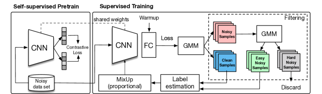
Figure 1: Our proposed PropMix has a self-supervised pre-training stage (Chen et al., 2020a; He et al., 2019; Chen et al., 2020b; Gansbeke et al., 2020), followed by a supervised training stage, where we first warm-up the classifier with a classification loss, using the pre-trained weights. Then, using the classification loss, we train a GMM to separate the samples into clean and noisy. Next, using classification confidence for the noisy set, we train a second GMM to separate the easy and hard noisy samples. The clean and easy noisy samples are proportionally combined in the MixUp for training.

After the pre-training, we warm-up the classifier by training it for a few epochs on the (noisy) training data set with the cross-entropy (CE) loss. The clean and noisy sets, $\mathcal{X},\mathcal{U}\subseteq\mathcal{D}$, are formed with (Arazo et al., 2019; Li et al., 2020; Lee et al., 2019b; Jiang et al., 2020):

$$\mathcal{X}=\left\{(\mathbf{x}_{i},\mathbf{y}_{i},w_{i}):w_{i}=p\left(\text{clean}|\ell_{i},\gamma\right)\geq\tau\right\},\quad\mathcal{U}=\left\{(\mathbf{x}_{i},\mathbf{y}_{i},w_{i}):w_{i}=p\left(\text{clean}|\ell_{i},\gamma\right)<\tau\right\},$$ (3)

with $\tau$ denoting a classification threshold, $\ell_{i}=-\mathbf{y}_{i}^{\top}\log p_{\theta}(.|f_{\phi}(\mathbf{x}_{i}))$, and $p\left(\text{clean}|\ell_{i},\gamma\right)$ being a function that estimates the probability that $(\mathbf{x}_{i},\mathbf{y}_{i})$ is a clean label sample. The function $p\left(\text{clean}|\ell_{i},\gamma\right)$ in Eq.3 is a bi-modal Gaussian mixture model (GMM) (Li et al., 2020), where $\gamma$ denotes the GMM parameters and the larger mean component is the noisy component whereas the smaller mean component is the clean component. Next, we obtain the sets of easy and hard noisy samples $\mathcal{U}_{E},\mathcal{U}_{H}\subseteq\mathcal{U}$, as follows:

$$\begin{split}\mathcal{U}_{E}&=\left\{(\mathbf{x}_{i},\mathbf{y}_{i}):p\left(\text{hard}|p_{\theta}(c_{i}^{*}|f_{\phi}(\mathbf{x})_{i}),\gamma\right)<\tau^{\prime}\right\},\\ \mathcal{U}_{H}&=\left\{(\mathbf{x}_{i},\mathbf{y}_{i}):p\left(\text{hard}|p_{\theta}(c_{i}^{*}|f_{\phi}(\mathbf{x}_{i})),\gamma\right)\geq\tau^{\prime}\right\},\end{split}$$ (4)

with $c_{i}^{*}=\operatorname*{arg\,max}_{c_{i}\in\mathcal{Y}}p_{\theta}(c_{i}|f_{\phi}(\mathbf{x}_{i}))$, $p\left(\text{hard}|p_{\theta}(c_{i}^{*}|f_{\phi}(\mathbf{x}_{i})),\gamma\right)$ being a function that estimates the probability that $(\mathbf{x}_{i},\mathbf{y}_{i})$ is a hard noisy label sample, and $\tau^{\prime}$ denoting the hard noisy sample threshold. The function $p\left(\text{hard}|p_{\theta}(c_{i}^{*}|f_{\phi}(\mathbf{x}_{i})),\gamma\right)$ in Eq. 4 is a GMM, where $\gamma$ denotes the GMM parameters and the smaller mean component is the hard noise component whereas the larger mean component is the easy noise component. We assume hard noisy samples have wrong label and wrong prediction, so we remove them from training.

Next, we perform $M$ data augmentations based on geometrical and visual transformations to increase the number of samples in $\mathcal{X}$ and $\mathcal{U}_{E}$, generating the augmented sets $\mathcal{X}^{\prime}=\{(\hat{\mathbf{x}}_{i},\hat{\mathbf{y}}_{i})\}_{i=1}^{|\mathcal{X}^{\prime}|}$ and $\mathcal{U}_{E}^{\prime}=\{(\hat{\mathbf{u}}_{i},\hat{\mathbf{q}}_{i})\}_{i=1}^{|\mathcal{U}_{E}^{\prime}|}$, with $\hat{\mathbf{x}}_{i}$ and $\hat{\mathbf{u}}_{i}$ being the augmented samples from $\mathcal{X}$ and $\mathcal{U}_{E}$, respectively, and $\hat{\mathbf{y}}_{i}$ and $\hat{\mathbf{q}}_{i}$ the label estimations defined as follows:

$$\hat{\mathbf{y}}_{i}=\text{TempShrp}(w_{i}\mathbf{y}_{i}+(1-w_{i})\mathbf{p}_{b};T),\quad\hat{\mathbf{q}}_{b}=\text{TempShrp}(\mathbf{q}_{b};T)$$ (5)

with $\mathbf{p}_{b}=\frac{1}{M}\sum\limits_{m=1}^{M}p_{\theta}(.|f_{\phi}(\hat{\mathbf{x}}_{i,m}))$, $\mathbf{q}_{b}=\frac{1}{M}\sum\limits_{m=1}^{M}p_{\theta}(.|f_{\phi}(\hat{\mathbf{u}}_{i}))$ , and TempShrp(.) being a temperature sharpening (Li et al., 2020).

The linear combination between the clean and easy noisy samples rely on MixUp (Zhang et al., 2017) data augmentation, which is different from the SOTA SSL approaches (Li et al., 2020) that use MixMatch (Berthelot et al., 2019) which has a training set size restricted by the clean set size. In particular, MixMatch-based methods select $B_{\mathcal{U}^{\prime}}=|\mathcal{X}^{\prime}|$ samples from the noisy set and $B_{\mathcal{X}^{\prime}}=|\mathcal{X}^{\prime}|$ samples from the clean set, so the MixUp proportion of samples from the noisy set is $\zeta=\frac{B_{\mathcal{U}^{\prime}}}{{B_{\mathcal{X}^{\prime}}+B_{\mathcal{U}^{\prime}}}}=0.5$, and the size of the MixMatch training set is $|\mathcal{X}^{\prime}|$. In our approach, we re-label the easy noisy samples in $\mathcal{U}^{\prime}_{E}$ and place them together with the clean samples in $\mathcal{X}^{\prime}$ for the MixUp data augmentation with $\mathcal{D}^{\prime}=\mathcal{X}^{\prime}\cup\mathcal{U}^{\prime}_{E}$. This operation enables us to obtain the proportionally mixed set $\hat{\mathcal{D}}=MixUp(\mathcal{D}^{\prime},\text{shuffled}(\mathcal{D}^{\prime}))$ where the proportion of samples from the noisy set, denoted by $\zeta=\frac{|\mathcal{U}^{\prime}_{E}|}{|\mathcal{X}^{\prime}|+|\mathcal{U}^{\prime}_{E}|}$, will be larger than $0.5$ for high noise rate problems.

To optimise the classification term we rely on the regularised CE loss (Li et al., 2020):

$$\mathcal{L}=\ell_{CE}+\lambda_{r}\ell_{r},$$ (6)

with $\ell_{CE}=-\frac{1}{|\mathcal{\hat{D}}|}\sum_{(\tilde{\mathbf{x}},\tilde{\mathbf{y}})\in\mathcal{\hat{D}}}\tilde{\mathbf{y}}^{\top}\log p_{\theta}(.|f_{\phi}(\tilde{\mathbf{x}}))$ and $\ell_{r}=KL\left[\pi_{|\mathcal{Y}|}\Bigg{|}\Bigg{|}\frac{1}{|\mathcal{\hat{D}}|}\sum_{(\mathbf{x},\mathbf{y})\in\mathcal{D}^{\prime}}p_{\theta}(.|f_{\phi}(\mathbf{x}))\right]$, where $\lambda_{r}$ weights the regularisation loss, and $\pi_{|\mathcal{Y}|}$ denotes a vector of $|\mathcal{Y}|$ dimensions with values equal to $1/|\mathcal{Y}|$. Different from SOTA semi-supervised methods (Li et al., 2020; Nishi et al., 2021), we do not have an additional loss for the noisy set because we assume that most of the samples in the noisy set have correct predictions (this is empirically shown in Sec. 4.3). A positive outcome from not using such additional loss for the noisy set is that we no longer need to manually set hyper-parameter values that depend on the noise rate of the problem, as is done by DivideMix (Li et al., 2020). The pseudo-code for the training of PropMix is shown in Algorithm 1 in the supplementary material.

4 Experiments

4.1 Data sets

We conduct our experiments on the data sets CIFAR-10, CIFAR-100 (Krizhevsky et al., 2009), Controlled Noisy Web Labels (CNWL) (Jiang et al., 2020), Clothing1M (Xiao et al., 2015) and WebVision (Li et al., 2017). CIFAR-10 and CIFAR-100 have 50k training and 10k testing images of size $32\times 32$ pixels, where CIFAR-10 has 10 classes and CIFAR-100 has 100 classes and all training and testing sets have equal number of images per classes. As CIFAR-10 and CIFAR-100 data sets originally do not contain label noise, we follow the literature (Li et al., 2020) and add the following synthetic noise types (see Sec. 3.1): symmetric (with noise rate $\eta\in\{0.2,0.5,0.8,0.9\}$, as defined in Sec. 3.1), asymmetric (using the mapping in (Li et al., 2020; Patrini et al., 2017), with $\eta_{jc}=0.4$), and semantic (Lee et al., 2019b) (with noisy labels based on a trained VGG (Simonyan and Zisserman, 2015), DenseNet (DN), and ResNet (RN)).

The CNWL dataset (Jiang et al., 2020) is a benchmark to study real-world web label noise in a controlled setting. Both images and labels are crawled from the web and the noisy labels are determined by matching images. The controlled setting provide different magnitudes of label corruption in real applications, varying from 0% to 80%. We study the red Mini-ImageNet that consists of 50k training images and 5k test images, with 100 classes. The original 84$\times$84-pixel images are resized to 32$\times$32 pixels. The noise rates are 20%, 60% and 80%, as used in (Xu et al., 2021).

Clothing1M consists of 1 million training images acquired from online shopping websites and it has 14 classes. As the images from the data set vary in size, we resized the images to $256\times 256$ for training, as used in Li et al. (2020); Han et al. (2019). The data set provide additional clean sets for training, validation, and testing of 50k, 14k and 10k images, respectively. For our experiments we do not use any of the clean training or validation sets, but we use the clean test set for evaluation.

WebVision contains 2.4 million images collected from the internet, with the same 1000 classes from ILSVRC12 (Deng et al., 2009) and images resized to $256\times 256$ pixels. It provides a clean test set of 50k images, with 50 images per class. We compare our model using the first 50 classes of the Google image subset, as used in Li et al. (2020); Chen et al. (2019).

4.2 Implementation

For CIFAR-10 and CIFAR-100 we used a 18-layer PreaAct-ResNet-18 (PRN18) (He et al., 2016) as our backbone model (Li et al., 2020). The models are trained with stochastic gradient descent (SGD) with momentum of 0.9, weight decay of 0.0005 and batch size of 64. For the self-supervised pre-training learning task, we adopt SimCLR (Chen et al., 2020a) with a batch size of 1024, SGD optimiser with a learning rate of 0.4, decay rate of 0.1, momentum of 0.9 and weight decay of 0.0001, and run it for 800 epochs. This pre-trained model produces feature representations of 128 dimensions. Using these representations we mine $K=20$ nearest neighbours (as in (Gansbeke et al., 2020)) for each sample to form the sets $\{\mathcal{N}_{\mathbf{x}_{i}}\}_{i=1}^{|\mathcal{D}|}$, defined in Sec. 3.2. In the supervised training stage, the model is trained with SGD with momentum of 0.9, weight decay of 0.0005 and batch size of 64. The learning rate is 0.02 which is reduced to 0.002 in the middle of the training. The WarmUp and total number of epochs is defined according to each data set, as defined in (Li et al., 2020). For CIFAR-10 and CIFAR-100, PRN18 is trained with a WarmUp stage of 30 epochs for CIFAR-10 and 10 epochs for CIFAR-100, and 300 epochs of final training. In our training, we also use a co-teaching approach, as in (Li et al., 2020; Liu et al., 2020a; Han et al., 2018b). We estimate noise rate with $|\mathcal{U}|/|\mathcal{D}|$, defined in Eq. 3 – if this ratio is larger than 50%, we use strong data augmentation with cutout (Cubuk et al., 2019), otherwise, we use standard augmentation (i.e., crop and flip).

For the semantic noise from (Lee et al., 2019b), we use DenseNet-100 (Iandola et al., 2014) as backbone, following (Lee et al., 2019b). The pre-training stage uses the same parameters as in CIFAR, except that we use a batch size of 512. In the supervised stage, we use the same protocol as (Lee et al., 2019b), which uses SGD with momentum 0.9, weight decay 10-4 and learning rate of 0.1 that is divided by 10 after epochs 40 and 80 for CIFAR-10 (which runs for 120 epochs in total), and after epochs 80, 120 and 160 for CIFAR-100 (runs for 200 epochs in total). The WarmUp epochs is the same as CIFAR-10/CIFAR-100.

For red Mini-Imagenet we use PRN18 as backbone, following (Xu et al., 2021). For the self-supervised pre-training task, we adopt SimCLR (Chen et al., 2020a) with batch size 128. All other parameters for the self-supervised pre-training are the same as described for CIFAR. For the supervised stage, we adopt the implementation of (Xu et al., 2021), where we train for 300 epochs, relying on SGD with learning rate of 0.02 (decreased by a factor of ten at epochs 200 and 250), momentum of 0.9 and weight decay of 5e-4.

For Clothing1M, we use ResNet-50 as backbone, following  (Li et al., 2020). In this protocol, a ResNet-50 with ImageNet (Deng et al., 2009) pre-trained weights is used and we decided to not use the self-supervised stage for this experiment because the model is already pre-trained. The ResNet-50 is trained for 80 epochs, including a WarmUp stage of 1 epoch, with a batch size of 32, SGD with a learning rate of 0.002 (divided by 10 at epoch 40), momentum of 0.9 and weight decay of 0.0001.

For Webvision, we use InceptionResNet-V2 as backbone, following (Li et al., 2020). For self-supervised pre-training, we adopt MoCo-v2 (4-GPU training) (Chen et al., 2020b), trained with 100 epochs, with a batch size of 128, SGD with a learning rate of 0.015 (divided by 10 at epoch 50), momentum of 0.9 and weight decay of 0.0001, and run it for 100 epochs with a WarmUp stage of 1 epoch. The feature representations learned from this process have 128 dimensions. All the other parameters were the same as described above for CIFAR.

4.3 PropMix Analysis

Fig. 2 shows the PropMix hard noisy sample filtering process for CIFAR-100 with 80% symmetric noise, at epoch 150 (i.e., half of the training epochs). The left histogram shows the clean and noisy classification from Eq. 3, while the right one shows the easy and hard noisy sample classification from Eq. (4). As can be seen, the use of confidence in Eq. (4), instead of the loss from Eq. 3, is an effective way to remove noisy samples with wrong prediction. We also evaluated the quality of the filtering stage using PropMix for CIFAR-100 under different symmetric noise rates. Fig. 3(a) and (b) show the precision and recall of the hard noisy sample filtering as a function of training epochs. These graphs show that the larger the noise, the higher the precision. For example, for 90% noise, the hard noise classification reaches 80% at the end of training. Fig. 3(c) shows the size of the noisy sample set during training. Fig. 3(d) compares the easy noise set re-labelling accuracy by PropMix with a baseline that does not filter out hard noisy samples. We can see that PropMix is substantially more accurate, which enables a more successful training with the easy noisy samples. We also evaluated the impact of the parameters $\tau$ and $\tau^{\prime}$ in the training. Fig. 4 shows the PropMix accuracy for CIFAR-10 (a-b) and CIFAR-100 (c-d) under different symmetric noise rates, varying the parameters $\tau$, which is related to the clean/noisy filtering from Eq. 3, and $\tau^{\prime}$, which related to hard noise filtering, from Eq. 4. Fig. 4(a,c) vary $\tau$ while fixing $\tau^{\prime}=0.5$, and Fig. 4(b,d) vary $\tau^{\prime}$ while fixing $\tau=0.5$. We can see that $\tau^{\prime}$ does not have a strong impact on the accuracy, which motivated us to use $\tau^{\prime}=0.5$ independently of the noise rate and data set. The parameter $\tau$ is shown to decrease accuracy at higher values. In PropMix we use $\tau=0.5$ as in other works Li et al. (2020).

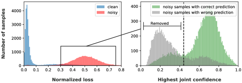
Figure 2: PropMix classification of easy and hard noisy samples. From the (normalized) loss of all samples, PropMix uses GMM to split clean and noisy samples, and then, using the largest classification confidence, it uses another GMM to split the hard and easy noisy samples. This example was run on CIFAR-100, 80% noise rate at epoch 150.

Figure 3: Evaluation of hard noisy sample filtering, for CIFAR-100, with 50% to 90% symmetric noise. Graphs in (a,b) show the precision and recall of the classification of hard noisy samples (i.e., noisy samples that are incorrectly labelled by the model), Graph (c) shows the estimated noise set size, and (d) shows the classification accuracy of the re-labelled easy noisy samples, compared to the baseline that does not filter out hard noisy samples.

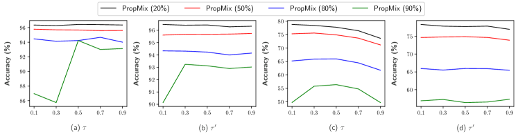
Figure 4: Evaluation of the parameters $\tau$ (clean sample threshold) and $\tau^{\prime}$ (hard noisy sample threshold), for CIFAR-10 and CIFAR-100, with 20% to 90% symmetric noise. Graphs in (a,b) show the best accuracy when training using PropMix with CIFAR-10, and graphs (c,d) show results for CIFAR-100, at different values of $\tau$ and $\tau^{\prime}$. Graph (a,c) vary the parameter $\tau$, while fixes $\tau^{\prime}$ at 0.5. Graph (b,d) vary the parameter $\tau^{\prime}$ while fixes $\tau$ at 0.5.

4.4 Comparison with State-of-the-Art

For CIFAR-10 and CIFAR-100, we evaluate our model using symmetric label noise ranging from 20% to 90%, and 40% asymmetric noise. We report both the best test accuracy across all epochs and the averaged test accuracy over the last 10 epochs of training, similar to (Li et al., 2020). Tab. 1 shows that for CIFAR-10 and CIFAR-100 data sets, our method obtains the best results for almost all evaluated noisy rates.

dataset		CIFAR-10					CIFAR-100
Noise type		sym.				asym.	sym.
Method/ noise ratio		20%	50%	80%	90%	40%	20%	50%	80%	90%
Cross-Entropy (Li et al., 2020)	Best	86.8	79.4	62.9	42.7	85.0	62.0	46.7	19.9	10.1
	Last	82.7	57.9	26.1	16.8	72.3	61.8	37.3	8.8	3.5
Coteaching+ (Yu et al., 2019)	Best	89.5	85.7	67.4	47.9	-	65.6	51.8	27.9	13.7
	Last	88.2	84.1	45.5	30.1	-	64.1	45.3	15.5	8.8
MixUp (Zhang et al., 2017)	Best	95.6	87.1	71.6	52.2	-	67.8	57.3	30.8	14.6
	Last	92.3	77.3	46.7	43.9	-	66.0	46.6	17.6	8.1
PENCIL (Yi and Wu, 2019)	Best	92.4	89.1	77.5	58.9	88.5	69.4	57.5	31.1	15.3
	Last	92.0	88.7	76.1	58.2	88.1	68.1	56.4	20.7	8.8
Meta-Learning (Li et al., 2019)	Best	92.9	89.3	77.4	58.7	89.2	68.5	59.2	42.4	19.5
	Last	92.0	88.8	76.1	58.3	88.6	67.7	58.0	40.1	14.3
M-correction (Arazo et al., 2019)	Best	94.0	92.0	86.8	69.1	87.4	73.9	66.1	48.2	24.3
	Last	93.8	91.9	86.6	68.7	86.3	73.4	65.4	47.6	20.5
MentorMix (Jiang et al., 2020)	Best	95.6	-	81.0	-	-	78.6	-	41.2	-
	Last	-	-	-	-	-	-	-	-	-
MOIT+ (Ortego et al., 2020)	Best	94.1	-	75.8	-	93.3	75.9	-	51.4	-
	Last	-	-	-	-	-	-	-	-	-
DivideMix (Li et al., 2020)	Best	96.1	94.6	93.2	76.0	93.4	77.3	74.6	60.2	31.5
	Last	95.7	94.4	92.9	75.4	92.1	76.9	74.2	59.6	31.0
ELR+ (Liu et al., 2020b)	Best	95.8	94.8	93.3	78.7	93.0	77.6	73.6	60.8	33.4
	Last	-	-	-	-	-	-	-	-	-
PropMix (Ours)	Best	96.44	95.77	93.94	93.48	94.89	77.41	74.56	67.34	58.57
	Last	96.09	95.53	93.77	93.20	94.64	76.99	73.71	66.75	58.32

Table 1: Test accuracy (%) for all competing methods on CIFAR-10 and CIFAR-100 under symmetric and asymmetric noises. Results from related approaches are as presented in (Li et al., 2020). Top methods within $1\%$ are in bold.

Tab. 2 shows the results for semantic noise (Lee et al., 2019b), which is harder and more realistic than the synthetic noise, where PropMix shows significantly more accurate results than any of the methods in (Lee et al., 2019b). In Tab. 5, we show that PropMix improves the SOTA by a large margin on the Red Mini-ImageNet semantic noise experiment from (Jiang et al., 2020).

Data set	CIFAR-10			CIFAR-100
Method/ noise ratio	DenseNet (32%)	ResNet (38%)	VGG (34%)	DenseNet (34%)	ResNet (37%)	VGG (37%)
D2L + RoG (Lee et al., 2019a)	68.57	60.25	59.94	31.67	39.92	45.42
CE + RoG (Lee et al., 2019a)	68.33	64.15	70.04	61.14	53.09	53.64
Bootstrap + RoG (Lee et al., 2019a)	68.38	64.03	70.11	54.71	53.30	53.76
Forward + RoG (Lee et al., 2019a)	68.20	64.24	70.09	53.91	53.36	53.63
Backward + RoG (Lee et al., 2019a)	68.66	63.45	70.18	54.01	53.03	53.50
PropMix (Ours)	84.25	82.51	85.74	60.98	58.44	60.01

Table 2: Test accuracy (%) for the semantic noise benchmark (Lee et al., 2019a), where baseline results are from (Lee et al., 2019a). The results with (*) were produced by locally running the published code provided by the authors. Top methods ($\pm 1\%$) are in bold.

We also evaluate PropMix on the noisy large-scale datasets WebVision (Li et al., 2017) and Clothing1M (Xiao et al., 2015). Tab. 5 shows competitive results compared to SOTA. As Clothing1M experimental protocol uses ImageNet pre-trained weights, the training could not benefit from PropMix strategy. Tab. 3 shows the Top-1/-5 test accuracy using the WebVision and ILSVRC12 test sets. Results show that PropMix is slightly better than the SOTA for WebVision test set. This suggests that our approach is also effective in large-scale, low noise rate problems.

4.5 Ablation Study

We show the ablation study of PropMix with CIFAR-10 and CIFAR-100 under symmetric and asymmetric noises at several rates. In Tab. 6, we show Self-superv. pre-train, which has the result from self-supervised training (with SCAN (Gansbeke et al., 2020)), where the result is the same across different noise rates because it never uses the noisy labels for training. SSL (DivideMix) (Li et al., 2020)) is current SOTA in noisy label learning, but it has worse accuracy in high noise rate problems (> 80% noise) than SCAN. Self-superv. pre-train+SSL (DivideMix) pre-trains DivideMix with SCAN to improve accuracy in high-noise rate problems, without affecting low-noise rate results. Just removing the MSE loss in Self-superv. pre-train+SSL (DivideMix) w/o MSE does not help much because the noisy samples from DivideMix is not accurately re-labelled. Adding our hard noisy sample filtering in Self-superv. pre-train+SSL (DivideMix) + filtering with MSE does not improve accuracy because DivideMix still uses MSE loss to train the easy noisy samples, which is unnecessary given that these samples are accurately re-labelled and can be trained with the CE loss. PropMix can achieve better results for high noise rates, using a simpler loss function (uses only CE loss) with less hyper-parameters, and removing hard noisy samples.

Method	Top-1	Top-5
F-correction (Patrini et al., 2017)	61.12	82.68
Decoupling (Malach and Shalev-Shwartz, 2017)	62.54	84.74
D2L (Ma et al., 2018)	62.68	84.00
MentorNet (Jiang et al., 2018)	63.00	81.40
Co-teaching (Han et al., 2018b)	63.58	85.20
Iterative-CV (Chen et al., 2019)	65.24	85.34
MentorMix (Jiang et al., 2020)	76.00	90.20
DivideMix (Li et al., 2020)	77.32	91.64
ELR+ (Liu et al., 2020a)	77.78	91.68
PropMix (Ours)	78.84	90.56

Table 3: Test accuracy (%) for WebVision (Li et al., 2017) by methods trained with 100 epochs. Baselines come from Li et al. (2020). Top methods within $1\%$ in bold.

Method/ noise ratio	20%	40%	60%	80%
Cross-entropy (Xu et al., 2021)	47.36	42.70	37.30	29.76
MixUp (Zhang et al., 2017)	49.10	46.40	40.58	33.58
DivideMix (Li et al., 2020)	50.96	46.72	43.14	34.50
MentorMix (Jiang et al., 2020)	51.02	47.14	43.80	33.46
FaMUS (Xu et al., 2021)	51.42	48.06	45.10	35.50
PropMix (Ours)	61.24	56.22	52.84	43.42

Table 4: Test accuracy (%) for Red Mini-ImageNet (Jiang et al., 2020). Results from baseline methods are as presented in (Xu et al., 2021). Top methods ($\pm 1\%$) are in bold.

Method	Test Accuracy
Cross-Entropy Li et al. (2020)	69.21
M-correction Arazo et al. (2019)	71.00
PENCILYi and Wu (2019)	73.49
DeepSelf Han et al. (2019)	74.45
CleanNet Lee et al. (2018)	74.69
DivideMix Li et al. (2020)	74.76
PropMix (ours)	74.30

Table 5: Test accuracy (%) for Clothing1M (Xiao et al., 2015) by methods trained with 80 epochs. Baselines come from Li et al. (2020). Top methods within $1\%$ are in bold.

dataset		CIFAR-10					CIFAR-100
Noise type		sym.				asym.	sym.
Method/ noise ratio		20%	50%	80%	90%	40%	20%	50%	80%	90%
Self-superv. pre-train (Gansbeke et al., 2020)		81.6	81.6	81.6	81.6	81.6	44.0	44.0	44.0	44.0
SSL (DivideMix) (Li et al., 2020)		96.1	94.6	93.2	76.0	93.4	77.3	74.6	60.2	31.5
Self-superv. pre-train + SSL (DivideMix)*		96.2	94.8	93.9	92.2	93.3	77.4	74.7	66.7	56.2
Self-superv. pre-train + SSL (DivideMix)* w/o MSE		96.2	95.2	91.4	85.1	93.3	77.2	73.9	62.6	52.1
Self-superv. pre-train + SSL (DivideMix)* + filtering with MSE		96.3	95.3	93.8	91.6	93.0	77.3	75.3	66.7	55.7
PropMix (Ours)		96.4	95.8	93.9	93.5	94.9	77.4	74.6	67.3	58.6

Table 6: In this ablation study we show the test accuracy (%) on CIFAR-10 and CIFAR-100 under symmetric and asymmetric noise problems. First, we show the results of self-supervised pre-training with SCAN (Gansbeke et al., 2020). Then we show the current SOTA SSL learning for noisy label DivideMix (Li et al., 2020). Next, we show the results of DivideMix pre-trained with SCAN. Then, we remove the MSE loss to train DivideMix re-labelled noisy samples, and add the hard noisy filtering stage (but keeping the MSE loss) to the pre-trained DivideMix. The last row shows our PropMix . The top results within $1\%$ are highlighted.

5 Conclusion and Future Work

We presented PropMix, a noisy label training algorithm to filter out hard noisy samples, remove samples with incorrect label and incorrect prediction from noisy set with the goal to keep the easy noisy samples that have a higher chance to be correctly re-labelled. PropMix reduces noisy-dependent parameters, while promoting the use of the entire filtered noisy set in a fully supervised training, with proportional MixUp data augmentation on the clean set. Our results on CIFAR-10/100, Red Mini-ImageNet, and WebVision outperform the SOTA methods, also demonstrating robustness to over-fitting in several noise rates with substantial improvement in high noise problems.

6 Acknowledgment

IR and GC gratefully acknowledge the support of the Australian Research Council through the Centre of Excellence for Robotic Vision CE140100016 and Future Fellowship (to GC) FT190100525. GC acknowledges the support by the Alexander von Humboldt-Stiftung for the renewed research stay sponsorship.

Appendix A PropMix Algorithm

SOTA noise-robust classifiers (Li et al., 2020; Nguyen et al., 2019; Liu et al., 2020a) are formed by an ensemble of two classifiers, where the classifier structure is the same, but their parameters are denoted by $\theta(1),\theta(2)\in\Theta$. The training for $\theta(1)$ influences $\theta(2)$ and vice-versa, where this can be achieved by co-training Li et al. (2020); Liu et al. (2020a) or student-teacher Nguyen et al. (2019) approaches. Our training relies on co-training. The estimation of class prediction for label estimation and evaluation are given by the average outputs of the models. The pseudo-code for the training of PropMix is shown in Algorithm 1.

1

Input: $\mathcal{D}$, number of epochs $E$, clean sample threshold $\tau$, hard sample threshold $\tau^{\prime}$

2

// Self-supervised pre-training

3 $f_{\phi}(\mathbf{x})$,$\{\mathcal{N}_{\mathbf{x}_{i}}\}_{i=1}^{|\mathcal{D}|}$ = PreTrain($\mathcal{D}$)

// Warm Up

4 $p_{\theta}(\mathbf{y}|\mathbf{x})$ = WarmUp($\mathcal{D}$,$f_{\phi}(\mathbf{x})$)

5 while $e<E$ do

       // Estimate sets of clean and noisy samples

6       for $i=\{1,...,|\mathcal{D}|\}$ do

7            Estimate $p(\text{clean}|\ell_{i},\gamma)$, with $\ell_{i}=-\mathbf{y}_{i}^{\top}\log p_{\theta}(.|\mathbf{x}_{i})$

8       end for

9      

10      $\mathcal{X},\mathcal{U}$=FormCleanNoisySets($\{p(\text{clean}|\ell_{i},\gamma)\}_{i=1}^{|\mathcal{D}|},\tau$)

      // Estimate sets of hard noisy and easy noisy samples

11       for $i=\{1,...,|\mathcal{U}|\}$ do

12            Estimate $p\left(\text{hard}|\mathbf{y}_{i}^{*}(c),\gamma\right)$, with $\mathbf{y}_{i}^{*}(c)=\operatorname*{arg\,max}_{c\in\mathcal{Y}}p\left(c|\mathbf{x}_{i}\right)$

13       end for

14      

15      $\mathcal{U}_{H},\mathcal{U}_{E}$=FormHardEasySets($\{p\left(\text{hard}|\mathbf{y}_{i}^{*}(c),\gamma\right)\}_{i=1}^{|\mathcal{U}|},\tau^{\prime}$) for b=1 to $B$ do

16            

17            $\{\hat{\mathbf{x}}_{b,m}\}_{m=1}^{M}$ = DataAugment($\mathbf{x}_{b}\in\mathcal{X},M$)

18             $\{\hat{\mathbf{u}}_{b,m}\}_{m=1}^{M}$ = DataAugment($\mathbf{u}_{b}\in\mathcal{U}_{E},M$)

19            $\mathbf{p}_{b}=\frac{1}{2M}\sum\limits_{m=1,k=1}^{M,2}f(\hat{\mathbf{x}}_{b,m};\theta(k))$

20             $\mathbf{q}_{b}=\frac{1}{2M}\sum\limits_{m=1,k=1}^{M,2}f(\hat{\mathbf{u}}_{b,m};\theta(k))$ $\hat{\mathbf{y}}_{b}=\text{TempShrp}(w_{b}\mathbf{y}_{b}+(1-w_{b})\mathbf{p}_{b};T)$

21             $\hat{\mathbf{q}}_{b}=\text{TempShrp}(\mathbf{q}_{b};T)$

22       end for

23      $\mathcal{\hat{X}}=\{\hat{\mathbf{x}}_{b,m},\hat{\mathbf{y}}_{b}\}_{m=1}^{M}$, $\mathcal{\hat{U}}_{E}=\{\hat{\mathbf{u}}_{b,m},\hat{\mathbf{q}}_{b}\}_{m=1}^{M}$

24       $\mathcal{\hat{D}}$ = ProportionalMixUp($\mathcal{\hat{X}},\mathcal{\hat{U}}_{E}$)

25       Update $\theta(k1)$, $\theta(k2)$ with $\mathcal{L}$ from (5)

26 end while

Algorithm 1 PropMix (PM)

References

- Aggarwal et al. (2021) Ravi Aggarwal, Viknesh Sounderajah, Guy Martin, Daniel SW Ting, Alan Karthikesalingam, Dominic King, Hutan Ashrafian, and Ara Darzi. Diagnostic accuracy of deep learning in medical imaging: a systematic review and meta-analysis. NPJ digital medicine, 4(1):1–23, 2021.
- Algan and Ulusoy (2021) Görkem Algan and Ilkay Ulusoy. Meta soft label generation for noisy labels. In 2020 25th International Conference on Pattern Recognition (ICPR), pages 7142–7148. IEEE, 2021.
- Arazo et al. (2019) Eric Arazo, Diego Ortego, Paul Albert, Noel O’Connor, and Kevin Mcguinness. Unsupervised label noise modeling and loss correction. In International Conference on Machine Learning, pages 312–321, 2019.
- Berthelot et al. (2019) David Berthelot, Nicholas Carlini, Ian Goodfellow, Nicolas Papernot, Avital Oliver, and Colin Raffel. MixMatch: A Holistic Approach to Semi-Supervised Learning. arXiv e-prints, art. arXiv:1905.02249, May 2019.
- Chen et al. (2019) Pengfei Chen, Benben Liao, Guangyong Chen, and Shengyu Zhang. Understanding and utilizing deep neural networks trained with noisy labels. arXiv preprint arXiv:1905.05040, 2019.
- Chen et al. (2020a) Ting Chen, Simon Kornblith, Mohammad Norouzi, and Geoffrey Hinton. A Simple Framework for Contrastive Learning of Visual Representations. arXiv e-prints, art. arXiv:2002.05709, February 2020a.
- Chen et al. (2020b) Xinlei Chen, Haoqi Fan, Ross Girshick, and Kaiming He. Improved Baselines with Momentum Contrastive Learning. arXiv e-prints, art. arXiv:2003.04297, March 2020b.
- Cubuk et al. (2019) Ekin D Cubuk, Barret Zoph, Dandelion Mane, Vijay Vasudevan, and Quoc V Le. Autoaugment: Learning augmentation strategies from data. In Proceedings of the IEEE/CVF Conference on Computer Vision and Pattern Recognition, pages 113–123, 2019.
- Deng et al. (2009) Jia Deng, Wei Dong, Richard Socher, Li-Jia Li, Kai Li, and Li Fei-Fei. Imagenet: A large-scale hierarchical image database. In 2009 IEEE conference on computer vision and pattern recognition, pages 248–255. Ieee, 2009.
- Ding et al. (2018) Yifan Ding, Liqiang Wang, Deliang Fan, and Boqing Gong. A semi-supervised two-stage approach to learning from noisy labels. In 2018 IEEE Winter Conference on Applications of Computer Vision (WACV), pages 1215–1224. IEEE, 2018.
- Frénay and Verleysen (2013) Benoît Frénay and Michel Verleysen. Classification in the presence of label noise: a survey. IEEE transactions on neural networks and learning systems, 25(5):845–869, 2013.
- Gansbeke et al. (2020) Wouter Van Gansbeke, Simon Vandenhende, Stamatios Georgoulis, Marc Proesmans, and Luc Van Gool. Scan: Learning to classify images without labels, 2020.
- Ghosh et al. (2017) Aritra Ghosh, Himanshu Kumar, and PS Sastry. Robust loss functions under label noise for deep neural networks. In Thirty-First AAAI Conference on Artificial Intelligence, 2017.
- Grigorescu et al. (2020) Sorin Grigorescu, Bogdan Trasnea, Tiberiu Cocias, and Gigel Macesanu. A survey of deep learning techniques for autonomous driving. Journal of Field Robotics, 37(3):362–386, 2020.
- Han et al. (2018a) Bo Han, Gang Niu, Jiangchao Yao, Xingrui Yu, Miao Xu, Ivor Tsang, and Masashi Sugiyama. Pumpout: A meta approach for robustly training deep neural networks with noisy labels. 2018a.
- Han et al. (2018b) Bo Han, Quanming Yao, Xingrui Yu, Gang Niu, Miao Xu, Weihua Hu, Ivor Tsang, and Masashi Sugiyama. Co-teaching: Robust training of deep neural networks with extremely noisy labels. In Advances in neural information processing systems, pages 8527–8537, 2018b.
- Han et al. (2019) Jiangfan Han, Ping Luo, and Xiaogang Wang. Deep self-learning from noisy labels. In Proceedings of the IEEE International Conference on Computer Vision, pages 5138–5147, 2019.
- He et al. (2016) Kaiming He, Xiangyu Zhang, Shaoqing Ren, and Jian Sun. Identity mappings in deep residual networks. In European conference on computer vision, pages 630–645. Springer, 2016.
- He et al. (2019) Kaiming He, Haoqi Fan, Yuxin Wu, Saining Xie, and Ross Girshick. Momentum Contrast for Unsupervised Visual Representation Learning. arXiv e-prints, art. arXiv:1911.05722, November 2019.
- Iandola et al. (2014) Forrest Iandola, Matt Moskewicz, Sergey Karayev, Ross Girshick, Trevor Darrell, and Kurt Keutzer. Densenet: Implementing efficient convnet descriptor pyramids. arXiv preprint arXiv:1404.1869, 2014.
- Jaehwan et al. (2019) Lee Jaehwan, Yoo Donggeun, and Kim Hyo-Eun. Photometric transformer networks and label adjustment for breast density prediction. In Proceedings of the IEEE International Conference on Computer Vision Workshops, pages 0–0, 2019.
- Jiang et al. (2018) Lu Jiang, Zhengyuan Zhou, Thomas Leung, Li-Jia Li, and Li Fei-Fei. Mentornet: Learning data-driven curriculum for very deep neural networks on corrupted labels. In International Conference on Machine Learning, pages 2304–2313, 2018.
- Jiang et al. (2020) Lu Jiang, Di Huang, Mason Liu, and Weilong Yang. Beyond synthetic noise: Deep learning on controlled noisy labels. ICML, 2020.
- Kim et al. (2019) Youngdong Kim, Junho Yim, Juseung Yun, and Junmo Kim. Nlnl: Negative learning for noisy labels. In Proceedings of the IEEE International Conference on Computer Vision, pages 101–110, 2019.
- Krizhevsky et al. (2009) Alex Krizhevsky, Geoffrey Hinton, et al. Learning multiple layers of features from tiny images. 2009.
- Lee et al. (2019a) Kimin Lee, Sukmin Yun, Kibok Lee, Honglak Lee, Bo Li, and Jinwoo Shin. Robust inference via generative classifiers for handling noisy labels. In International Conference on Machine Learning, pages 3763–3772. PMLR, 2019a.
- Lee et al. (2019b) Kimin Lee, Sukmin Yun, Kibok Lee, Honglak Lee, Bo Li, and Jinwoo Shin. Robust inference via generative classifiers for handling noisy labels. arXiv preprint arXiv:1901.11300, 2019b.
- Lee et al. (2018) Kuang-Huei Lee, Xiaodong He, Lei Zhang, and Linjun Yang. Cleannet: Transfer learning for scalable image classifier training with label noise. In Proceedings of the IEEE Conference on Computer Vision and Pattern Recognition, pages 5447–5456, 2018.
- Li et al. (2019) Junnan Li, Yongkang Wong, Qi Zhao, and Mohan S Kankanhalli. Learning to learn from noisy labeled data. In Proceedings of the IEEE Conference on Computer Vision and Pattern Recognition, pages 5051–5059, 2019.
- Li et al. (2020) Junnan Li, Richard Socher, and Steven C. H. Hoi. DivideMix: Learning with Noisy Labels as Semi-supervised Learning. arXiv e-prints, art. arXiv:2002.07394, February 2020.
- Li et al. (2017) Wen Li, Limin Wang, Wei Li, Eirikur Agustsson, and Luc Van Gool. Webvision database: Visual learning and understanding from web data. arXiv preprint arXiv:1708.02862, 2017.
- Litjens et al. (2017) Geert Litjens, Thijs Kooi, Babak Ehteshami Bejnordi, Arnaud Arindra Adiyoso Setio, Francesco Ciompi, Mohsen Ghafoorian, Jeroen Awm Van Der Laak, Bram Van Ginneken, and Clara I Sánchez. A survey on deep learning in medical image analysis. Medical image analysis, 42:60–88, 2017.
- Liu et al. (2020a) Sheng Liu, Jonathan Niles-Weed, Narges Razavian, and Carlos Fernandez-Granda. Early-learning regularization prevents memorization of noisy labels. arXiv preprint arXiv:2007.00151, 2020a.
- Liu et al. (2020b) Sheng Liu, Jonathan Niles-Weed, Narges Razavian, and Carlos Fernandez-Granda. Early-learning regularization prevents memorization of noisy labels. arXiv preprint arXiv:2007.00151, 2020b.
- Ma et al. (2018) Xingjun Ma, Yisen Wang, Michael E Houle, Shuo Zhou, Sarah Erfani, Shutao Xia, Sudanthi Wijewickrema, and James Bailey. Dimensionality-driven learning with noisy labels. In International Conference on Machine Learning, pages 3355–3364, 2018.
- Ma et al. (2020) Xingjun Ma, Hanxun Huang, Yisen Wang, Simone Romano, Sarah Erfani, and James Bailey. Normalized loss functions for deep learning with noisy labels. In International Conference on Machine Learning, pages 6543–6553. PMLR, 2020.
- Malach and Shalev-Shwartz (2017) Eran Malach and Shai Shalev-Shwartz. Decoupling" when to update" from" how to update". In Advances in Neural Information Processing Systems, pages 960–970, 2017.
- Miao et al. (2015) Qiguang Miao, Ying Cao, Ge Xia, Maoguo Gong, Jiachen Liu, and Jianfeng Song. Rboost: Label noise-robust boosting algorithm based on a nonconvex loss function and the numerically stable base learners. IEEE transactions on neural networks and learning systems, 27(11):2216–2228, 2015.
- Minaee et al. (2021) Shervin Minaee, Yuri Y Boykov, Fatih Porikli, Antonio J Plaza, Nasser Kehtarnavaz, and Demetri Terzopoulos. Image segmentation using deep learning: A survey. IEEE Transactions on Pattern Analysis and Machine Intelligence, 2021.
- Nguyen et al. (2019) Duc Tam Nguyen, Chaithanya Kumar Mummadi, Thi Phuong Nhung Ngo, Thi Hoai Phuong Nguyen, Laura Beggel, and Thomas Brox. Self: Learning to filter noisy labels with self-ensembling. arXiv preprint arXiv:1910.01842, 2019.
- Nishi et al. (2021) Kento Nishi, Yi Ding, Alex Rich, and Tobias Höllerer. Augmentation Strategies for Learning with Noisy Labels. arXiv e-prints, art. arXiv:2103.02130, March 2021.
- Ortego et al. (2019) Diego Ortego, Eric Arazo, Paul Albert, Noel E O’Connor, and Kevin McGuinness. Towards robust learning with different label noise distributions. arXiv preprint arXiv:1912.08741, 2019.
- Ortego et al. (2020) Diego Ortego, Eric Arazo, Paul Albert, Noel E O’Connor, and Kevin McGuinness. Multi-objective interpolation training for robustness to label noise. arXiv preprint arXiv:2012.04462, 2020.
- Patrini et al. (2017) Giorgio Patrini, Alessandro Rozza, Aditya Krishna Menon, Richard Nock, and Lizhen Qu. Making deep neural networks robust to label noise: A loss correction approach. In Proceedings of the IEEE Conference on Computer Vision and Pattern Recognition, pages 1944–1952, 2017.
- Pleiss et al. (2020) Geoff Pleiss, Tianyi Zhang, Ethan R Elenberg, and Kilian Q Weinberger. Identifying mislabeled data using the area under the margin ranking. arXiv preprint arXiv:2001.10528, 2020.
- Ren et al. (2018) Mengye Ren, Wenyuan Zeng, Bin Yang, and Raquel Urtasun. Learning to reweight examples for robust deep learning. In International Conference on Machine Learning, pages 4334–4343, 2018.
- Simonyan and Zisserman (2015) Karen Simonyan and Andrew Zisserman. Very deep convolutional networks for large-scale image recognition. ICLR, 2015.
- Song et al. (2019) Hwanjun Song, Minseok Kim, and Jae-Gil Lee. Selfie: Refurbishing unclean samples for robust deep learning. In International Conference on Machine Learning, pages 5907–5915. PMLR, 2019.
- Wang et al. (2019a) Xinshao Wang, Yang Hua, Elyor Kodirov, and Neil M Robertson. Imae for noise-robust learning: Mean absolute error does not treat examples equally and gradient magnitude’s variance matters. arXiv preprint arXiv:1903.12141, 2019a.
- Wang et al. (2020) Xinshao Wang, Yang Hua, Elyor Kodirov, and Neil M Robertson. Proselflc: Progressive self label correction for training robust deep neural networks. arXiv e-prints, pages arXiv–2005, 2020.
- Wang et al. (2019b) Yisen Wang, Xingjun Ma, Zaiyi Chen, Yuan Luo, Jinfeng Yi, and James Bailey. Symmetric cross entropy for robust learning with noisy labels. In Proceedings of the IEEE International Conference on Computer Vision, pages 322–330, 2019b.
- Xiao et al. (2015) Tong Xiao, Tian Xia, Yi Yang, Chang Huang, and Xiaogang Wang. Learning from massive noisy labeled data for image classification. In Proceedings of the IEEE conference on computer vision and pattern recognition, pages 2691–2699, 2015.
- Xu et al. (2021) Youjiang Xu, Linchao Zhu, Lu Jiang, and Yi Yang. Faster meta update strategy for noise-robust deep learning. In CVPR, 2021.
- Yi and Wu (2019) Kun Yi and Jianxin Wu. Probabilistic end-to-end noise correction for learning with noisy labels. In Proceedings of the IEEE Conference on Computer Vision and Pattern Recognition, pages 7017–7025, 2019.
- Yu et al. (2019) Xingrui Yu, Bo Han, Jiangchao Yao, Gang Niu, Ivor W Tsang, and Masashi Sugiyama. How does disagreement help generalization against label corruption? arXiv preprint arXiv:1901.04215, 2019.
- Yuan et al. (2018) Bodi Yuan, Jianyu Chen, Weidong Zhang, Hung-Shuo Tai, and Sara McMains. Iterative cross learning on noisy labels. In 2018 IEEE Winter Conference on Applications of Computer Vision (WACV), pages 757–765. IEEE, 2018.
- Zhang et al. (2016) Chiyuan Zhang, Samy Bengio, Moritz Hardt, Benjamin Recht, and Oriol Vinyals. Understanding deep learning requires rethinking generalization. arXiv preprint arXiv:1611.03530, 2016.
- Zhang et al. (2017) Hongyi Zhang, Moustapha Cisse, Yann N Dauphin, and David Lopez-Paz. mixup: Beyond empirical risk minimization. arXiv preprint arXiv:1710.09412, 2017.