Model, sample, and epoch-wise descents: exact solution of gradient flow in the random feature model

Abstract

Recent evidence has shown the existence of a so-called double-descent and even triple-descent behavior for the generalization error of deep-learning models. This important phenomenon commonly appears in implemented neural network architectures, and also seems to emerge in epoch-wise curves during the training process. A recent line of research has highlighted that random matrix tools can be used to obtain precise analytical asymptotics of the generalization (and training) errors of the random feature model. In this contribution, we analyze the whole temporal behavior of the generalization and training errors under gradient flow for the random feature model. We show that in the asymptotic limit of large system size the full time-evolution path of both errors can be calculated analytically. This allows us to observe how the double and triple descents develop over time, if and when early stopping is an option, and also observe time-wise descent structures. Our techniques are based on Cauchy complex integral representations of the errors together with recent random matrix methods based on linear pencils.

1 Introduction

Deep learning models have vastly increased in terms of number of parameters in the architecture and data sample sizes with recent applications using unprecedented numbers with as much as 175 billions parameters trained over billions of tokens [1]. Such massive amounts of data and growing training budgets have spurred research seeking empirical power laws to scale model sizes appropriately with available resources [2], and nowadays it is common wisdom among practitioners that "larger models are better". This ongoing trend has been challenging classical statistical modeling where it is thought that increasing the number of parameters past an interpolation threshold (at which the training error vanishes while the test error usually increases) is doomed to over-fit the data [3]. We refer to [4] for a recent extensive discussion on this contradictory state of affairs. Progress towards rationalizing this situation came from a series of papers [5, 6, 7, 8, 9, 10, 11] evidencing the existence of phases where increasing the number of parameters beyond the interpolation threshold can actually achieve good generalization, and the characteristic ${\rm U}$ curve of the bias-variance tradeoff is followed by a "descent" of the generalization error. This phenomenon has been called the double descent and was analytically corroborated in linear models [12, 13, 14, 15, 16] as well as random feature (RF) (or random feature regression) shallow network models [17, 18, 19, 20]. Many of these works provide rigorous proofs with precise asymptotic expressions of double descent curves. Further developments have brought forward rich phenomenology, for example, a triple-descent phenomenon [21] linked to the degree of non-linearity of the activation function. Further empirical evidence [22] has also shown that a similar effect occurs while training (ResNet18s on CIFAR10 trained using Adam) and has been called epoch-wise double descent. Moreover the authors of [22] extensively test various CIFAR data sets, architectures (CNNs, ResNets, Transformers) and optimizers (SGD, Adam) and classify their observations into three types of double descents: (i) model-wise double descent when the number of network parameters is varied; (ii) sample-wise double descent when the data set size is varied; and (iii) epoch-wise double descent which occurs while training. We wish to note that sample-wise double descent was derived long ago in precursor work on single layer perceptron networks [23, 24]. An important theoretical challenge is to unravel all these structures in a unified analytical way and understand how generalization error evolves in time.

In this contribution we achieve a detailed analytical analysis of the gradient flow dynamics of the RF model (or regression) in the high-dimensional asymptotic limit. The model was initially introduced in [25] as an approximation of kernel machines; more recently it has been recognized as an important playground for theoretical analysis of the model-wise double descent phenomenon, using tools from random matrix theory [17, 18, 26]. Following [17] we view the RF model as a $2$-layer neural network with fixed-random-first-layer-weights and dynamical second layer learned weights. The data is given by $n$ training pairs constituted of $d$-dimensional input vectors and output given by a linear function with additive gaussian noise. The data is fed through $N$ neurons with a non-linear activation function and followed by one linear neuron whose weights we learn by gradient descent over a quadratic loss function. The high-dimensional asymptotic limit is defined as the regime $n,d,N\to+\infty$ while the ratios tend to finite values $\frac{N}{d}\to\psi$ and $\frac{n}{d}\to\phi$. As the training loss is convex one expects that the least-squares predictor (with Moore-Penrose inversion) gives the long time behavior of gradient descent. This has led to the calculation of highly non-trivial analytical algebraic expressions for training and generalization errors which describe (model-wise and sample-wise) double and triple descent curves [17, 21]. However, to the best of our knowledge, there is no complete analytical derivation of the whole time evolution of the two errors.

We analyze the gradient flow equations in the high-dimensional regime and deduce the whole time evolution of the training and generalization errors. Numerical simulations show that the gradient flow is an excellent approximation of gradient descent in the high-dimensional regime as long as the step size is small enough (see Fig. 2). Main contributions presented in detail in Sect. 3 comprise:

a. Results 3.1 and 3.2 give expressions of the time evolution of the errors in terms of one and two-dimensional integrals over spectral densities whose Stieltjes transforms are given by a closed set of purely algebraic equations. The expressions lend themselves to numerical computation as illustrated in Fig. 1 and more extensively in Sect. 3 and the supplementary material.

b. Model and sample-wise double descents develop after some definite time at the interpolation threshold and are preceded by a dip or minimum before the spike develops. This indicates that early stopping is beneficial for some parameter regimes. A similar behavior also occurs for the triple descent. (See Figs. 3, 4 and the 3D version Fig. 1).

c. We observe two kinds of epoch-wise "descent" structures. The first is a double plateau monotonously descending structure at widely different time scales in the largely overparameterized regime (see Fig. 3). The second is an epoch-wise double descent similar to the one found in [22]. In fact, as in [22], rather than a spike, this double descent appears to be an elongated bump over a wide time scale (see Fig. 5 and the 3D version Fig. 1).

Let us say a few words about the techniques used in this work. We first translate the gradient flow equations for the learned weights of the second layer into a set of integro-differential equations for generating functions, as in [27], involving the resolvent of a random matrix (constructed out of the fixed first layer weights, the data, and the non-linear activation). The solution of the integro-differential equations and the time evolution of the errors can then be expressed in terms of Cauchy complex integral representation which has the advantage to decouple the time dependence and static contributions involving traces of algebraic combinations of standard random matrices (see [28] for related methods). This is the content of propositions 2.0.1 and 2.0.2. With a natural concentration hypothesis in the high-dimensional regime, it remains to carry out averages over the static traces involving random matrices. This is resolved using traces of sub-blocks from the inverse of a larger nontrivial block-matrix, a so-called linear pencil. To the best of our knowledge linear pencils have been introduced in the machine learning community only recently in [29]. This theory is developed in the context of random matrix theory in [30, 31] and [32] using operator valued free-probability. A side-contribution in the SM is also an independent (but non-rigorous) derivation of a basic result of this theory (a fixed point equation) using a replica symmetric calculation from statistical physics. The non-linearity of the activation function is addressed using the gaussian equivalence principle [33, 34, 29]. Finally, our analysis is not entirely mathematically controlled mainly due to the concentration hypothesis in Sect. 2.3 but comparison with simulations (see Fig. 2 and SM) confirm that the analytical results are exact.

In the conclusion we briefly discuss possible extensions of the present analysis and open problems among which is the comparison with a dynamical mean-field theory approach.

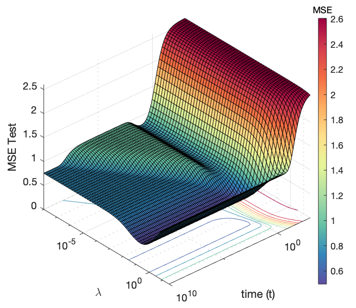
(a)

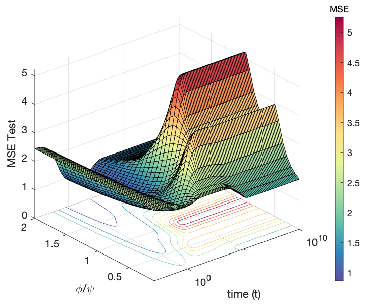
(b)

Figure 1: 3D plot of analytical test error evolution. See Figs. 5 and 4 (on the right) for parameter values.

2 Random feature model

2.1 Model description

Generative model and neural network:

We consider the problem of learning a linear function $f_{d}(x)=d^{-\frac{1}{2}}\beta^{T}x$ with $x,\beta\in\mathbb{R}^{d}$ column vectors. The vector $x$ is interpreted as a random input and $\beta$ as a random hidden vector; both with distribution $\mathcal{N}(0,I_{d})$, $I_{d}$ the $d\times d$ identity matrix. We assume having access to the hidden function through the noisy outputs $y=f_{d}(x)+\epsilon$ with additive gaussian noise $\epsilon\sim\mathcal{N}(0,s^{2})$, $s\in\mathbb{R}_{+}$. We suppose that we have $n$ data-points $(x_{i},y_{i})_{1\leq i\leq n}$. This data can be represented as the $n\times d$ matrix $X\in\mathbb{R}^{n\times d}$ where $x_{i}^{T}$ is the $i$-th row of $X$, and the column vector vector $Y\in\mathbb{R}^{n}$ with $i$-th entry $y_{i}$. Therefore, we have the matrix notation $Y=d^{-\frac{1}{2}}X\beta+\xi$ where $\xi\sim\mathcal{N}(0,s^{2}I_{n})$ and $I_{n}$ the $n\times n$ identity matrix.

We learn the data with a shallow $2$-layer neural network. There are $N$ hidden neurons with weight (column) vectors $\theta_{i}\in\mathbb{R}^{d}$, $i=1,\cdots,N$ each connected to the $d$ input neurons. Out of these we form the matrix (of the first layer connecting input and hidden neurons) $\Theta\in\mathbb{R}^{N\times d}$ where $\theta_{i}^{T}$ is the $i$-th row of $\Theta$ . Its entries are assumed independent and sampled through a standard gaussian distribution $\mathcal{N}(0,1)$; they are not learned but fixed once for all. The data-points in $X$ are applied linearly to the parameters $\Theta$, and the output $Z\in\mathbb{R}^{n\times N}$ of the first layer is the pointwise application of an activation function $\sigma:\mathbb{R}\to\mathbb{R}$, $Z=\sigma(d^{-\frac{1}{2}}X\Theta^{T})$. We use the notation $z_{i}^{T}$ to express the $i$-th row of $Z$. The second layer consists in a weight (column) vector $a_{t}\in\mathbb{R}^{N}$ to be learned, indexed by time $t\geq 0$, with components initially sampled at $t=0$ i.i.d $\mathcal{N}(0,r^{2})$, $r\in\mathbb{R}_{+}$. The prediction vector is expressed as $\hat{Y}_{t}=N^{-\frac{1}{2}}Za_{t}$.

We assume that the activation function belongs to $L^{2}(e^{-\frac{x^{2}}{2}}dx)$ with inner product denoted $\langle\,,\,\rangle$. It can be expanded on the basis of Hermite polynomials, so $\sigma\in\text{Span}\left((H_{e_{k}})_{k\geq 0}\right)$, where $H_{e_{k}}(x)=(-1)^{k}e^{\frac{x^{2}}{2}}\frac{d^{k}}{dx^{k}}e^{-\frac{x^{2}}{2}}$ (so $H_{e_{0}}(x)=1$, $H_{e_{1}}(x)=x$, $H_{e_{2}}(x)=x^{2}-1$, $H_{e_{3}}(x)=x^{3}-3x$, …). Furthermore we take $\sigma$ centered with $\langle\sigma,H_{e_{0}}\rangle=0$, and set $\mu=\langle\sigma,H_{e_{1}}\rangle$, $\nu^{2}=\langle\sigma,\sigma\rangle-\mu^{2}$. For instance, $\sigma=\text{id}$ has $(\mu,\nu)=(1,0)$ while $\sigma=\text{Relu}-\frac{1}{\sqrt{2\pi}}$ has $(\mu,\nu)=(\frac{1}{2},\frac{1}{2}(1-\frac{2}{\pi})^{1/2})\simeq(0.5,0.3)$. Finally, we recall that we are interested in the high dimensional regime where the parameters $N,n,d$ tend to infinity with the ratios $\frac{N}{d}\to\psi$ and $\frac{n}{d}\to\phi$.

Training and test errors:

For a new input $x_{0}\in\mathbb{R}^{d}$, we define the predictor $\hat{y}_{t}(x_{0})=\frac{1}{\sqrt{N}}z(x_{0})^{T}a_{t}$ where $z(x_{0})=\sigma(\frac{1}{\sqrt{d}}\Theta x_{0})$. We will further define the standard training and test errors with a penalization term $\lambda>0$ and the quadratic loss:

$$\mathcal{H}^{\text{train}}(a)=\frac{1}{n}\left\lVert Y-\hat{Y}\right\rVert^{2}+\frac{\lambda}{N}\left\lVert a\right\rVert^{2},\quad\mathcal{H}^{\text{test}}(a)=\mathbb{E}_{x_{0}\sim\mathcal{N}(0,1)}{\left[(y(x_{0})-\hat{y}(x_{0}))^{2}\right]}$$ (1)

Note that because of the $\lambda$-penalization term, in this context, the training error can be above the test error in some configurations of parameters. Also, we will slightly abuse this notation throughout the paper by using $\mathcal{H}^{\text{train}}_{t},\mathcal{H}^{\text{test}}_{t}$ to designate $\mathcal{H}^{\text{train}}(a_{t}),\mathcal{H}^{\text{test}}(a_{t})$.

Gradient flow:

Minimizing the training error of this shallow-network is equivalent to a standard Tikhonov regularization problem with a design matrix $Z$ for which the optimal weights are given by $a_{\infty}=(\frac{Z^{T}Z}{N}+\frac{n}{N}\lambda I_{N})^{-1}\frac{Z^{T}}{\sqrt{N}}Y$. The errors generated by the predictors with weights $a_{\infty}$ have been analytically calculated in the high-dimensional regime in [17] and further analyzed in [21]. Here we study the whole time evolution of the gradient flow and thus introduce an additional time dimension in our model. Of course as $t\to+\infty$ one recovers the errors generated by the predictors with weights $a_{\infty}$. The output vector $a_{t}$ is updated through the ordinary differential equation $\frac{da_{t}}{dt}=-\eta\nabla_{a}\mathcal{H}^{\text{train}}(a_{t})$ with a fixed learning rate parameter $\eta>0$. As $\eta$ can be absorbed in the time parameter, from now on we consider without loss of generality that $\eta=\frac{n}{2}$. Setting $\delta=\lambda\frac{n}{N}$, we find that the gradient flow for $a_{t}$ is a first order linear matrix differential equation,

$$\frac{da_{t}}{dt}=-\left(\frac{Z^{T}Z}{N}+\delta I_{N}\right)a_{t}+\frac{Z^{T}Y}{\sqrt{N}}.$$ (2)

Recall the initial condition $a_{0}$ is a vector with i.i.d $\mathcal{N}(0,r^{2})$ components.

2.2 Cauchy integral representations of the training and test errors

An important step of our analysis is the representation of $\mathcal{H}^{\text{train}}$ and $\mathcal{H}^{\text{test}}$ in terms of Cauchy contour integrals in the complex plane. To this end we decompose both errors in elementary contributions and derive contour integrals for each of them. Details are found in section 4 and the SM.

We begin with the test error which is more complicated. We have

$$\mathcal{H}^{\text{test}}_{t}=1+s^{2}-2\mu g(t)+\mu^{2}h(t)+\nu^{2}l(t)+o_{d}(1)$$ (3)

where $\lim_{d\to+\infty}o_{d}(1)=0$ with high probability, and $g(t)=\frac{\beta^{T}}{\sqrt{d}}\frac{\Theta^{T}}{\sqrt{d}}\frac{a_{t}}{\sqrt{N}}$, $h(t)=\|\frac{\Theta^{T}}{\sqrt{d}}\frac{a_{t}}{\sqrt{N}}\|^{2}$, and $l(t)=\|\frac{a_{t}}{\sqrt{N}}\|^{2}$. To describe Cauchy’s integral representation of the elementary functions $g$, $h$, $l$ we introduce the resolvent $R(z)=(\frac{Z^{T}Z}{N}-zI_{N})^{-1}$ for all $z\in\mathbb{C}\setminus\text{Sp}(\frac{Z^{T}Z}{N})$.

Proposition 2.0.1 (Test error)

Let $\mathcal{R}_{z}$ be the functional acting on holomorphic functions $f:\mathbb{C}\setminus\text{Sp}(\frac{Z^{T}Z}{N})\rightarrow\mathbb{C}$ as $\mathcal{R}_{z}\{f(z)\}=-\oint_{\Gamma}\frac{\mathrm{d}z}{2\pi i}f(z)$ over a contour $\Gamma$ encircling the spectrum $\text{Sp}(\frac{Z^{T}Z}{N})$ in the counterclockwise direction. Similarly, let $\mathcal{R}_{x,y}$ be the functional acting on two-variable holomorphic functions $f:(\mathbb{C}\setminus\text{Sp}(\frac{Z^{T}Z}{N}))^{2}\rightarrow\mathbb{C}$ as $\mathcal{R}_{x,y}\{f(x,y)\}=\oint_{\Gamma}\oint_{\Gamma}\frac{\mathrm{d}x}{2\pi i}\frac{\mathrm{d}y}{2\pi i}f(x,y)$. Let $G_{t}(z)=\frac{\beta^{T}}{\sqrt{d}}\frac{\Theta^{T}}{\sqrt{d}}R(z)\frac{a_{t}}{\sqrt{N}}$ and $K(z)=\frac{\beta^{T}}{\sqrt{d}}\frac{\Theta^{T}}{\sqrt{d}}R(z)\frac{Z^{T}Y}{N}$. We have for all $t\geq 0$

$$g(t)=\mathcal{R}_{z}\left\{e^{-t(z+\delta)}G_{0}(z)+\frac{1-e^{-t(z+\delta)}}{z+\delta}K(z)\right\}.$$ (4)

Let $L_{t}(z)=\frac{a_{t}^{T}}{\sqrt{N}}R(z)\frac{a_{t}}{\sqrt{N}}$ and $U_{t}(z)=\frac{Y^{T}Z}{N}R(z)\frac{a_{t}}{\sqrt{N}}$ and $V(z)=\frac{Y^{T}Z}{N}R(z)\frac{Z^{T}Y}{N}$. For all $t\geq 0$

$$l(t)\!=\!\mathcal{R}_{z}\!\left\{e^{-2t(z+\delta)}L_{0}(z)\!+\!2e^{-t(z+\delta)}\left(\frac{1-e^{-t(z+\delta)}}{\delta+z}\right)U_{0}(z)\!+\!\left(\frac{1-e^{-t(\delta+z)}}{\delta+z}\right)^{2}V(z)\right\}\!.$$ (5)

Let $H_{t}(x,y)=\frac{a_{t}^{T}}{\sqrt{N}}R(x)\frac{\Theta\Theta^{T}}{d}R(y)\frac{a_{t}}{\sqrt{N}}$, $Q_{t}(x,y)=\frac{a_{t}^{T}}{\sqrt{N}}R(x)\frac{\Theta\Theta^{T}}{d}R(y)\frac{Z^{T}Y}{N}$ and $W(x,y)=\frac{Y^{T}Z}{N}R(x)\frac{\Theta\Theta^{T}}{d}R(y)\frac{Z^{T}Y}{N}$. For all $t\leq 0$

$$h(t) =\mathcal{R}_{x,y}\left\{e^{-t(2\delta+x+y)}\left(\frac{e^{t(\delta+y)}-1}{\delta+y}Q_{0}(x,y)+\frac{e^{t(\delta+x)}-1}{\delta+x}Q_{0}(y,x)\right)\right\}$$

$$+\mathcal{R}_{x,y}\left\{\frac{1-e^{-t(x+\delta)}}{x+\delta}\frac{1-e^{-t(y+\delta)}}{y+\delta}W(x,y)\right\}+\mathcal{R}_{x,y}\left\{e^{-t(x+y+2\delta)}H_{0}(x,y)\right\}.$$ (6)

A similar but much simpler representation holds for the training error.

Proposition 2.0.2 (Training error)

With the same definitions than in proposition 2.0.1 we have

$$\mathcal{H}^{\text{train}}_{t}\!=\!\frac{\left\lVert Y\right\rVert^{2}}{n}\!+\!\frac{1}{c}\mathcal{R}_{z}\!\left\{(z+\delta)e^{-2t(z+\delta)}L_{0}(z)\!-\!2e^{-2t(z+\delta)}U_{0}(z)\!-\!\frac{1-e^{-2t(\delta+z)}}{\delta+z}V(z)\!\right\}.$$ (7)

2.3 High-dimensional framework

The Cauchy integral representation involves a set of one-variable functions $\mathcal{S}_{1}=\{G_{0},K,L_{0},U_{0},V\}:\mathbb{C}\setminus\text{Sp}(\frac{Z^{T}Z}{N})\to\mathbb{C}$ and a set of two-variable functions $\mathcal{S}_{2}=\{H_{0},W,Q_{0}\}:\mathbb{C}\setminus\text{Sp}(\frac{Z^{T}Z}{N}))^{2}\to\mathbb{C}$ so that $g$, $h$, $l$ and thus also $\mathcal{H}^{\text{test}}$ and $\mathcal{H}^{\text{train}}$ are actually functions of $(t;\mathcal{S}_{1},\mathcal{S}_{2})$. Thus we can write for instance: $\mathcal{H}^{\text{test}}(a_{t})=\mathcal{H}^{\text{test}}(t;\mathcal{S}_{1},\mathcal{S}_{2})$. We simplify the problem by considering the high-dimensional regime where $N,n,d\to\infty$ with ratios $\frac{N}{d}\to\psi$, $\frac{n}{d}\to\phi$ tending to fixed values of order one. In this regime we expect that the functions in $\mathcal{S}_{1}$ and $\mathcal{S}_{2}$ concentrate and can therefore be replaced by their averages over randomness. These averages can be carried out using recent progress in random matrix theory [30], [31], and we are able to compute pointwise asymptotic values of the functions in $\mathcal{S}_{1}$, $\mathcal{S}_{2}$, and eventually substitute them in the Cauchy integral representations for the training and test error. In general, rigorously showing concentration of the various functions involved is not easy and we will make the following assumptions:

Assumptions 2.1

In the high dimensional limit with $d,N,n\to\infty$ and $\frac{N}{d}\to\psi$, $\frac{n}{d}\to\phi$:

1. The random functions in $\mathcal{S}_{1}$, $\mathcal{S}_{2}$ are assumed to concentrate. We let $\bar{\mathcal{S}}_{1}=\{\bar{G}_{0},\bar{K},\bar{L}_{0},\bar{U}_{0},\bar{V}\}$ and $\bar{\mathcal{S}}_{2}=\{\bar{H}_{0},\bar{W},\bar{Q}_{0}\}$ be the pointwise limit of the functions.

2. There exists a bounded subset $\mathcal{C}\subset\mathbb{R}^{+}$ such that the functions in $\bar{\mathcal{S}}_{1}$ and $\bar{\mathcal{S}}_{2}$ are holomorphic on $\mathbb{C}\setminus\mathcal{C}$ and $(\mathbb{C}\setminus\mathcal{C})^{2}$ respectively

3. The gaussian equivalence principle (see sect. 4.2) can be applied to the limiting quantities.

It is common that the closure of the spectrum of suitably normalized random matrices concentrates on a deterministic set. Thus the bounded set $\mathcal{C}$ can be understood as the limit of the finite interval $[0,\lim_{d}\max\text{Sp}(\frac{Z^{T}Z}{N})]$. In the sequel we will distinguish the theoretical high-dimensional regime from the finite dimensional regime using the upper-bar notation.

Definition 2.1 (High-dimensional framework)

Under the assumptions 2.1, we define the theoretical test error $\bar{\mathcal{H}}^{\text{test}}_{t}=\mathcal{H}^{\text{test}}(t;\bar{\mathcal{S}}_{1},\bar{\mathcal{S}}_{2})$ and the theoretical training error $\bar{\mathcal{H}}^{\text{train}}_{t}=\mathcal{H}^{\text{train}}(t;\bar{\mathcal{S}}_{1},\bar{\mathcal{S}}_{2})$

We conjecture that $\lim_{d}\mathcal{H}^{\text{train}}_{t}=\bar{\mathcal{H}}^{\text{train}}_{t}$ and $\lim_{d}\mathcal{H}^{\text{test}}_{t}=\bar{\mathcal{H}}^{\text{test}}_{t}$ at all time $t\in\mathbb{R}$. We verify that this conjecture stands experimentally for sufficiently large $d$ on different configurations (see additional figures in the SM). This also lends experimental support on the assumption 2.1. Furthermore we conjecture that the $d\to+\infty$ and $t\to\infty$ limits commute, namely $\lim_{d}\lim_{t}\mathcal{H}^{\text{train}}_{t}=\lim_{t}\bar{\mathcal{H}}^{\text{train}}_{t}$ and $\lim_{d}\lim_{t}\mathcal{H}^{\text{test}}_{t}=\lim_{t}\bar{\mathcal{H}}^{\text{test}}_{t}$.

3 Results and insights

3.1 Main results

In this section we provide the main results of this work: analytical formulas tracking the test and training errors during gradient flow of the random feature model for all times in the high-dimensional theoretical framework.

Result 3.1

Under the assumption 2.1, the theoretical test and training errors of definition 2.1 are given for all times $t\geq 0$ by the formulas

$$\bar{\mathcal{H}}^{\text{test}}_{t}=1+s^{2}-2\mu\bar{g}(t)+\mu^{2}\bar{h}(t)+\nu^{2}\bar{l}(t),$$ (8)

$$\bar{\mathcal{H}}^{\text{train}}_{t}=1+s^{2}+\frac{1}{c}\int_{\mathbb{R}}\left[(\delta+\omega)e^{-2t(\omega+\delta)}\rho_{\bar{L}_{0}}(\omega)-\frac{1-e^{-2t(\delta+\omega)}}{\delta+\omega}\rho_{\bar{V}}(\omega)\right]\mathrm{d}\omega,$$ (9)

with $c=\frac{\phi}{\psi}$, $\delta=c\lambda$, and the functions $\bar{g}$, $\bar{h}$, $\bar{l}$ given by

$$\bar{g}(t)=\int_{\mathbb{R}}\frac{1-e^{-t(\omega+\delta)}}{\omega+\delta}\rho_{\bar{K}}(\omega)\mathrm{d}\omega,$$ (10)

$$\bar{l}(t)=\int_{\mathbb{R}}\left[e^{-2t(\omega+\delta)}\rho_{\bar{L}_{0}}(\omega)+\left(\frac{1-e^{-t(\omega+\delta)}}{\omega+\delta}\right)^{2}\rho_{\bar{V}}(\omega)\right]\mathrm{d}\omega,$$ (11)

$$\bar{h}(t)=\iint_{\mathbb{R}^{2}}\left[e^{-t(u+v+2\delta)}\rho_{\bar{H}_{0}}(u,v)+\frac{1-e^{-t(u+\delta)}}{u+\delta}\frac{1-e^{-t(v+\delta)}}{v+\delta}\rho_{\bar{W}}(u,v)\right]\mathrm{d}u\mathrm{d}v,$$ (12)

where the measures $\rho_{\bar{K}},\rho_{\bar{L}_{0}},\rho_{\bar{V}},\rho_{\bar{H}_{0}},\rho_{\bar{W}}$ (are possibly signed) are characterized by their Stieltjes transforms given by $\bar{K},\bar{L}_{0},\bar{V},\bar{H}_{0},\bar{W}$

$$\begin{cases}\bar{K}(x)=t_{1}^{x},\quad\bar{L}_{0}(x)=r^{2}g_{1}^{x},\quad\bar{V}(x)=s^{2}\left(1+xg_{1}^{x}\right)+\left(c-h_{4}^{x}\right),\\ \bar{H}_{0}(x,y)=r^{2}q_{1},\quad\bar{W}(x,y)=s^{2}cq_{4}+q_{2}\end{cases}$$ (13)

where for each $x,y\in\mathbb{C}^{+}$ (the upper half complex plane) $g_{1}^{x},h_{4}^{x},t_{1}^{x},g_{1}^{y},h_{4}^{y},t_{1}^{y}$ and $q_{1},q_{2},q_{4},q_{5}$ (which depend symmetrically on $(x,y)$, e.g., $q_{1}=q_{1}^{x,y}=q_{1}^{y,x}$) are solutions of a purely algebraic system of equations (see SM for the criterion to select the relevant solution)

$$\left\{\begin{array}[]{l}0=\mu\psi g_{1}^{x}h_{4}^{x}-t_{1}^{x}\\ 0=\mu\psi g_{1}^{y}h_{4}^{y}-t_{1}^{y}\\ 0=(c-1-xg_{1}^{x})\left(c-\mu^{2}\phi g^{x}_{1}h^{x}_{4}\right)-ch^{x}_{4}\\ 0=(c-1-yg_{1}^{y})\left(c-\mu^{2}\phi g^{y}_{1}h^{y}_{4}\right)-ch^{y}_{4}\\ 0=1-g^{x}_{1}\left(\mu^{2}h^{x}_{4}+(c-1-xg_{1}^{x})\nu^{2}-x\right)\\ 0=1-g^{y}_{1}\left(\mu^{2}h^{y}_{4}+(c-1-yg_{1}^{y})\nu^{2}-y\right)\\ 0=-\mu^{2}g^{y}_{1}q_{2}+\mu^{2}h^{x}_{4}q_{1}+\mu g^{y}_{1}t^{x}_{1}+\mu g^{y}_{1}t^{y}_{1}-cg^{y}_{1}q_{4}\nu^{2}-g^{y}_{1}-q_{1}x+q_{1}\nu^{2}\left(c-g^{x}_{1}x-1\right)\\ 0=\mu\left(\phi-\psi g^{x}_{1}x-\psi\right)\left(-\mu g^{x}_{1}q_{2}+\mu h^{y}_{4}q_{1}+g^{x}_{1}t^{y}_{1}\right)+cq_{4}(1-\mu t_{1}^{y})-q_{2}\\ 0=-\mu^{2}\phi g^{x}_{1}(1-\mu t_{1}^{x})q_{4}+\mu^{2}q_{5}\left(c-g^{y}_{1}y-1\right)-\nu^{2}\phi g^{x}_{1}q_{4}-\phi q_{4}+q_{1}\nu^{2}\left(\phi-\psi g^{y}_{1}y-\psi\right)\\ 0=\psi(\mu^{2}\phi g^{x}_{1}g^{y}_{1}q_{4}+\psi g^{x}_{1}g^{y}_{1}+q_{1})(1-\mu t_{1}^{y})-\mu^{2}\psi g^{x}_{1}q_{5}\left(c-g^{x}_{1}x-1\right)-q_{5}\end{array}\right.$$

We can also deduce the limiting training error and test errors in the infinite time limit:

Result 3.2

In the limit $t\to\infty$ we find:

$$\lim_{t\to\infty}\bar{\mathcal{H}}^{\text{test}}_{t}\!=\!1+s^{2}-2\mu\bar{K}(-\delta)+\mu^{2}\bar{W}(-\delta,-\delta)+\nu^{2}\frac{\mathrm{d}\bar{V}}{\mathrm{d}x}(-\delta),\,\,\lim_{t\to\infty}\bar{\mathcal{H}}^{\text{train}}_{t}\!=\!1+s^{2}-\frac{1}{c}\bar{V}(-\delta)$$

Interestingly, in the limit $t\to\infty$, the expressions become simpler and completely algebraic in the sense that we do not need to compute integrals (or double-integrals) over the supports of the eigenvalue distributions. It is not obvious to see on the analytical expressions that the result is the same as the algebraic expressions obtained in [17] but Fig. 2 shows an excellent match with simulation experiments. We note here that checking that two sets of complicated algebraic equations are equivalent is in general a non-trivial problem of computational algebraic geometry [35].

3.2 Insights and illustrations of results

The set of analytical formulas allows to compute numerically the measures $\rho_{K},\rho_{L_{0}},\rho_{V},\rho_{H_{0}},\rho_{W}$ and in turn the full time evolution of the test and training errors. The result matches the simulation of a large random feature model where $d$ is taken large as can be seen on Figs. 2 for the infinite time limit (experimental check of result 3.2) and additional figures in the SM (experimental check of result 3.1). Below we illustrate numerical computations obtained with analytical formulas of result 3.1 for various sets of parameters $(t,\mu,\nu,\psi,\phi,r,s,\lambda)$. For instance, we can freely choose two of these parameters and plot the generalization error in 3D as in Fig. 1, or as a heat-map in the following. We describe three important phenomena which are observed with our analysis.

Double descent and early-stopping benefits: while [17] mostly analyze the minimum least-squares estimator of the random feature model which displays the double-descent at $\psi=\phi$, we are predicting the whole time evolution of the gradient flow as in Fig. 3. We clearly observe the double-descent curve at $t=10^{10}$ for $\psi=\phi$; but we now notice that if we stop the training earlier, say at times $1<t<10$, the generalization error performs better than the minimum least squares estimator. Actually, in the time interval $t\in(1,10)$ for $\psi\approx\phi$ the test error even has a dip or minimum just before the spike develops. We also notice a two-steps descent structure with the test error which is non-existent in the training error and materializes long after the training error has stabilized in the overparameterized regime $\psi\gg\phi$. This is also reminiscent but not entirely similar to the abrupt grokking phenomenon described in [36].

Triple descent: We can observe a triple descent phenomenon materialized by two spikes as seen in Fig. 2 at $t=\infty$ (we also check that the theoretical result matches very well the empirical prediction of the minimum least squares estimator both for training and test errors). This triple descent phenomenon is already contained in the formulas of [17] (although not discussed in this reference) and has been analyzed in detail in [21]. The test error contains a so-called linear spike for $\phi=1$ ($n=d$) and a non-linear spike for $\psi=\phi$ ($N=n$). The two spikes are often not seen together as this requires certain conditions to be met, and they tend to materialize together for specific values $\mu$, $\nu$ of the activation function where $\mu\gg\nu$. Here we further observe the evolution through time of the triple descent and the two spikes and how they develop in Fig. 4. There, we notice that the linear-spike seems to appear earlier than the non-linear one.

Epoch-wise descent structures: Important phenomena that we uncover here are two time-wise "descent structures". (i) As can be seen in Fig. 3, the test error develops a double plateau structure at widely different time scales in the over-parameterized regime ($\psi\gg\phi$) while there seems to be only one time scale for the training error. This kind of double plateau descent is different from the "usual" double-descent. (ii) Moreover, on Fig. 5 for well chosen parameters (in particular for noises with $s$ and $r$ "larger" and $\psi=2\phi$), we can also observe an elongated bump (rather than a thin spike) for small $\lambda$’s. Notice the logarithmic time-scale which clearly shows that here we need to wait exponentially longer to attain the "second descent" after the bump. This is very reminiscent of the epoch-wise double descent described in [22] for deep networks (which happens on similar time scales).

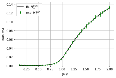
(a)

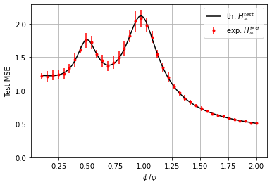
(b)

Figure 2: Large time limit. Analytical training error and test error profile with parameters $(\mu,\nu,\psi,r,s,\lambda)=(10,1,2,1,0.5,0.01)$ compared with experimental least squares MSE with $40$ data-points with $d=5000$ (average of 10 instances with confidence bar at $2\sigma$)

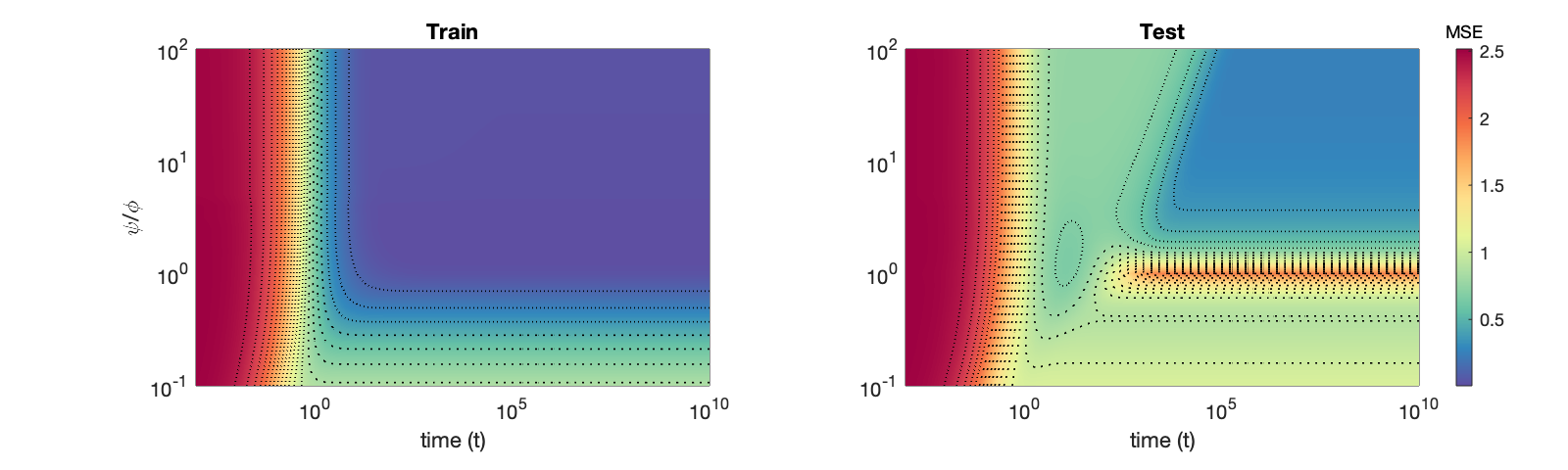
Figure 3: Model-wise double descent. Analytical training error and test error evolution with parameters $(\mu,\nu,\phi,r,s,\lambda)=(0.5,0.3,3,2.,0.4,0.001)$. Note that we vary the number of model parameters ($\psi$).

Figure 4: Sample-wise descents. Analytical training error and test error evolution with parameters $(\mu,\nu,\psi,r,s,\lambda)=(0.9,0.1,2,1,0.8,0.0001)$. Note that we vary the number of samples ($\phi$).

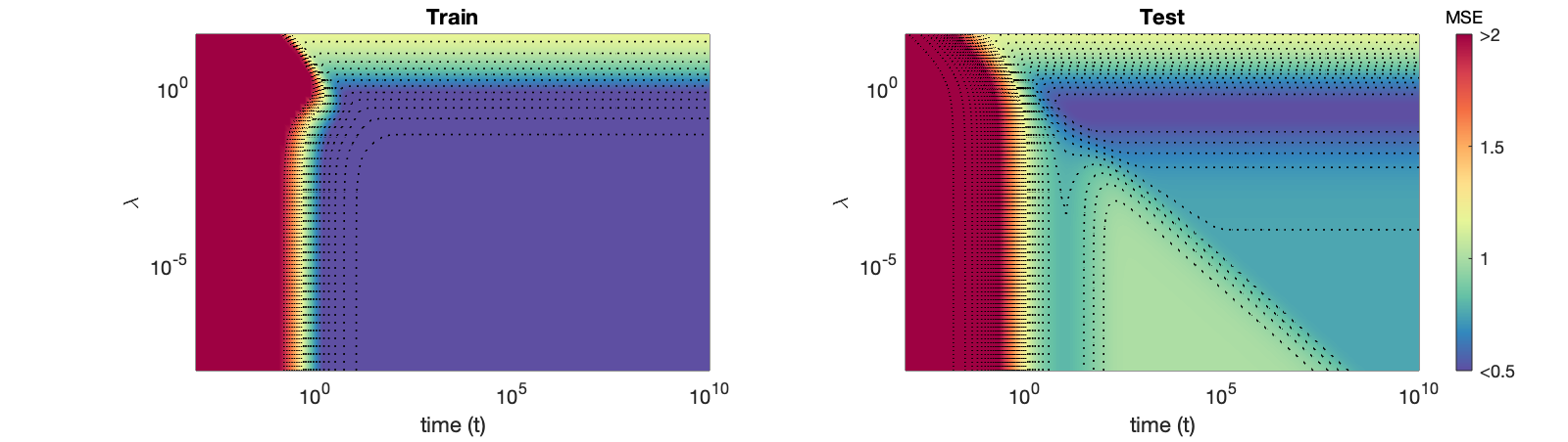
Figure 5: Epoch-wise descent structures. Analytical test error evolution with respect to different values of $\lambda$ $(\mu,\nu,\psi,\phi,r,s)=(0.5,0.3,6,3,2.0,0.5)$. Here the ratio of number of parameters and samples is fixed.

4 Sketch of proofs and analytical derivations

The analysis is threefold. Firstly, we decompose the training and test errors in elementary terms and establish Cauchy’s integral representation for each of them, as provided in proposition 2.0.1. A crucial advantage of this form is that it dissociates a scalar time-wise component and static matrix terms. Secondly, we switch to the high-dimensional framework where the matrix terms are substituted by their limit using the gaussian equivalence principle. Thirdly, we can compute the expectations of matrix terms thanks to a random matrix technique based on linear pencils. In this section we only sketch the main ideas for each step and provide details in the supplementary material.

4.1 Cauchy’s integral representation

We sketch the derivation for the test error and leave details to appendices. The derivation for the training error is entirely found in the SM. Expanding the square in Equ. (1) and carrying out averages we find Equ. (3) for $\mathcal{H}^{\text{test}}_{t}$ with $g(t)=\frac{\beta^{T}}{\sqrt{d}}\frac{\Theta^{T}}{\sqrt{d}}\frac{a_{t}}{\sqrt{N}}$, $h(t)=\|\frac{\Theta^{T}}{\sqrt{d}}\frac{a_{t}}{\sqrt{N}}\|^{2}$, and $l(t)=\|\frac{a_{t}}{\sqrt{N}}\|^{2}$ (see SM for this derivation).

We show how to derive the Cauchy integral representation for $g(t)$. For $h(t)$, $l(t)$ the steps are similar and found in SM. Let us consider the function $(t,z)\mapsto G_{t}(z)$ as in 2.0.1. Then we have the relation $g(t)=\frac{-1}{2i\pi}\oint_{\Gamma}\mathrm{d}zG_{t}(z)$ where $\Gamma$ is a loop in $\mathbb{C}$ enclosing the spectrum of $\frac{Z^{T}Z}{N}$. This can easily be seen by decomposing the symmetric $\frac{Z^{T}Z}{N}$ in an orthonormal basis $v_{1},\ldots,v_{N}$ with the eigenvalues $\lambda_{1},\ldots,\lambda_{N}$: then we have $G_{t}(z)=\sum_{i=1}^{N}\frac{1}{\lambda_{i}-z}\left(\frac{\beta^{T}}{\sqrt{d}}\frac{\Theta^{T}}{\sqrt{d}}v_{i}v_{i}^{T}\frac{a_{t}}{\sqrt{N}}\right)$ and because $\lambda_{i}$ are all encircled by $\Gamma$, we find $-\oint_{\Gamma}\frac{\mathrm{d}z}{2\pi i}G_{t}(z)=\sum_{i=1}^{N}\frac{\beta^{T}}{\sqrt{d}}\frac{\Theta^{T}}{\sqrt{d}}v_{i}v_{i}^{T}\frac{a_{t}}{\sqrt{N}}=g(t)$. Now, the ODE derived for $a_{t}$ in (2), can be written slightly differently using the fact that $\frac{Z^{T}Z}{N}=R(z)^{-1}+zI$ for any $z$ outside $\text{Sp}(\frac{Z^{T}Z}{N})$. Namely, $\frac{da_{t}}{dt}=\frac{Z^{T}Y}{\sqrt{N}}-R(z)^{-1}a_{t}-(z+\delta)a_{t}$. Then, we can derive an integro-differential equation for $G_{t}(z)$ involving $g(t)$ and $K(z)$:

$$\frac{\partial_{t}G_{t}(z)}{\partial t}=K(z)-g(t)-(z+\delta)G_{t}(z)$$ (14)

In the following, we let $\mathcal{L}$ be the Laplace transform operator $(\mathcal{L}f)(p)=\int_{0}^{+\infty}dt\,e^{-pt}f(t)$, $\operatorname{Re}p$ large enough. Note that the contour integral is performed over a compact set $\Gamma$ so for $\operatorname{Re}p$ large enough, by Fubini’s theorem, the operations $\mathcal{L}$ and $\mathcal{R}_{z}$ commute. Applying $\mathcal{L}$ to (14) and rearranging terms we find for $\operatorname{Re}(p+z+\delta)\neq 0$:

$$\mathcal{L}G_{p}(z)=\frac{G_{0}(z)}{p+z+\delta}+\frac{K(z)}{p(p+z+\delta)}-\frac{\mathcal{L}g(p)}{p+z+\delta}$$ (15)

Now, we can always choose $\Gamma$ such that $-(p+\delta)$ is outside of the contour if we assume $\operatorname{Re}(p+\delta)>0$ (since $\min_{i}\lambda_{i}\geq 0$). Thus, applying $\mathcal{R}_{z}$ to (15) nullifies the last term because the pole is outside $\Gamma$, and using commutativity $\mathcal{R}_{z}\mathcal{L}G_{p}=\mathcal{L}\mathcal{R}_{z}G_{p}$,

$$\mathcal{R}_{z}\mathcal{L}G_{p}=\mathcal{L}\mathcal{R}_{z}\left\{e^{-t(z+\delta)}G_{0}(z)+\frac{1-e^{-t(z+\delta)}}{z+\delta}K(z)\right\}=\mathcal{L}g(p).$$ (16)

Finally, using the inverse Laplace transform leads to (4).

4.2 Gaussian equivalence principle

The matrix terms must be estimated in the limit $d\to\infty$ with $\{\beta,a_{0},\xi,\Theta,X\}$ all independently distributed. As per assumptions 2.1 all the matrix terms in $\mathcal{S}_{1},\mathcal{S}_{2}$ are assumed to concentrate. So for instance we assume that the following limit exists $\bar{K}(z)\equiv\lim_{d\to\infty}K(z)=\lim_{d\to\infty}\mathbb{E}_{\beta,\xi,\Theta,X}[K(z)]$. Using cyclicity of the trace we easily perform averages over $\beta,\xi$ to find

$$\bar{K}(z)=\lim_{d}\mathbb{E}_{\beta,\Theta,X}\text{Tr}\left[\frac{\Theta^{T}}{\sqrt{d}}R(z)\frac{Z^{T}X}{N}\frac{\beta\beta^{T}}{d}\right]=\lim_{d}\frac{1}{d}\mathbb{E}_{\beta,\Theta,X}\text{Tr}\left[\frac{\Theta^{T}}{\sqrt{d}}R(z)\frac{Z^{T}X}{N}\right].$$ (17)

After these reductions, the expressions of all functions in $\bar{\mathcal{S}}_{1},\bar{\mathcal{S}}_{2}$ essentially involve products of random matrices $\Theta$, $X$ and pointwise applications of the non-linear activation $\sigma$. This can be further reduced to simpler algebraic expressions using the gaussian equivalence principle. This principle states that: there exists a standard gaussian random matrix $\Omega\in\mathbb{R}^{n\times N}$ independent of $\{X,\Theta\}$ such that in the infinite dimensional limit we can make the substitution $Z=\sigma\left(d^{-1/2}X\Theta^{T}\right)\longrightarrow\mu d^{-1/2}X\Theta^{T}+\nu\Omega$ in the expressions of all functions in $\bar{\mathcal{S}}_{1},\bar{\mathcal{S}}_{2}$. This approach is quite general and is well described in [29, 37] (and formerly in [33] and [34]). Thus it remains to compute expectations of traces containing only products, and inverses of products and sums, of gaussian matrices.

4.3 Expectations over random matrices using linear pencils

We explain how to compute the limit of (17) once the gaussian equivalence principle has been applied. A powerful approach is to design a so-called linear pencil. In the present context this is a suitable block-matrix containing gaussian random matrices and multiples of the identity matrix, for which full block-inversion gives back the products of terms in the traces that are being sought. This approach has been described in [30, 31, 38]. We have found a suitable linear pencil which contains fortuitously all the terms required in $\bar{\mathcal{S}}_{1},\bar{\mathcal{S}}_{2}$. It is described by the $13\times{13}$ block-matrix $M$, and pursuing with our example, we get for instance with the block $(7,12)$ that $\lim_{d}K(y)=\lim_{d}\frac{1}{d}{\rm Tr}[(M^{-1})^{(7,12)}]$

$$\begin{array}[]{c}M\!=\!\!\left[\!\begin{array}[]{ccccccccccccc}-xI&-\mu\frac{\Theta}{\sqrt{d}}&-I&0&0&0&\frac{\Theta}{\sqrt{d}}&0&0&0&0&0&0\\ 0&I&0&\frac{X^{T}}{\sqrt{N}}&0&0&0&0&0&0&0&0&0\\ 0&0&I&\nu\frac{\Omega^{T}}{\sqrt{N}}&0&0&0&0&0&0&0&0&0\\ 0&0&0&I&\frac{X}{\sqrt{N}}&\nu\frac{\Omega}{\sqrt{N}}&0&0&0&0&0&0&0\\ \mu\frac{\Theta^{T}}{\sqrt{d}}&0&0&0&I&0&0&0&0&0&0&0&0\\ I&0&0&0&0&I&0&0&0&0&0&0&0\\ 0&0&0&0&0&0&I&0&0&0&0&0&\frac{\Theta^{T}}{\sqrt{d}}\\ 0&0&0&0&0&0&0&I&0&\nu\frac{\Omega^{T}}{\sqrt{N}}&0&0&0\\ 0&0&0&0&0&0&0&0&I&\frac{X^{T}}{\sqrt{N}}&0&0&0\\ 0&0&0&0&0&0&0&0&0&I&\nu\frac{\Omega}{\sqrt{N}}&\frac{X}{\sqrt{N}}&0\\ 0&0&0&0&0&0&0&0&0&0&I&0&-I\\ 0&0&0&0&0&0&0&0&0&0&0&I&-\mu\frac{\Theta^{T}}{\sqrt{d}}\\ 0&0&0&0&0&0&0&I&\mu\frac{\Theta}{\sqrt{d}}&0&0&0&-yI\\ \end{array}\!\right]\end{array}$$

Next, the great advantage of the linear pencil is that (as described in [30, 31, 38]) it allows to write a fixed point equation $F(G)=G$ for a "small" $13\times{13}$ matrix $G$ with scalar matrix elements. We also provide in the SM an independent derivation of the fixed point equations using the replica method (a technique from statistical physics [39]).The components of $G$ are linked to the limiting traces of the blocks of $M^{-1}$ as in $[G]_{2,7}=\bar{K}(z)$. The action of $F$ can be completely described as an algebraic function leading to (a priori) $13\times 13=169$ equations over the matrix elements of $G$. The number of equations can be immediately reduced to $39$ because many elements vanish, and with the help of a computer algebra system the number of equations can be further brought down to $10$. We refer to the SM for all the details about the method.

5 Conclusion

We believe that our analysis could be extended to study the learning of non-linear functions, the effect of multilayered structures, and potentially different layers such as convolutions, as long as they are not learned. A challenging task is to extend the present methods to learned multilayers. A further question is the application of our analysis in teacher-student scenarios with realistic datasets (See [40, 37]).

Finally we wish to point out that a comparison of the approach of the present paper (and the similar but simpler one of [27]) with the dynamical mean-field theory (DMFT) approach of statistical physics remains to be investigated. DMFT has a long history originating in studies of complex systems (turbulent fluids, spin glasses) where one eventually derives a set of complicated integro-differential equations for suitable correlation and response functions capturing the whole dynamics of the system (we refer to the recent book [41] and references therein). This is a powerful formalism but the integral equations must usually be solved entirely numerically which itself is not a trivial task. For problems close to the present context (neural networks,generalized linear models, phase retrieval) DMFT has been developed in the recent works [42, 43, 44, 45, 46]. We think that comprehensively comparing this formalism with the present approach is an interesting open problem. It would be desirable to connect the DMFT equations to our closed form solutions for the training and generalization errors expressed in terms of a set of algebraic equations of suitable Stieltjes transforms.

Appendix A Test Error substitutions

The test error $\mathcal{H}^{\text{test}}_{t}$ in (1) can be expanded into smaller terms

$$\mathcal{H}^{\text{test}}_{t} =\mathbb{E}_{x_{0}}[y(x_{0})^{2}]-2\mathbb{E}_{x_{0}}[y(x_{0})\hat{y}_{t}(x_{0})]+\mathbb{E}_{x_{0}}[\hat{y}_{t}(x_{0})^{2}]$$

$$=\mathbb{E}_{x_{0}}[y(x_{0})^{2}]-2\frac{\beta^{T}}{\sqrt{d}}\mathbb{E}_{x_{0}}[x_{0}z(x_{0})^{T}]\frac{a_{t}}{\sqrt{N}}+\frac{a_{t}^{T}}{\sqrt{N}}\mathbb{E}_{x_{0}}[z(x_{0})z(x_{0})^{T}]\frac{a_{t}}{\sqrt{N}}.$$ (18)

The random noise $\epsilon$ from $y(x_{0})$ only impacts the first term on the right hand side with $\mathbb{E}_{x_{0}}[y(x_{0})^{2}]=1+s^{2}$. Using further $q(t)=\frac{\beta^{T}}{\sqrt{d}}\mathbb{E}_{x_{0}}[x_{0}z(x_{0})^{T}]\frac{a_{t}}{\sqrt{N}}$ and $p(t)=\frac{a_{t}^{T}}{\sqrt{N}}\mathbb{E}_{x_{0}}[z(x_{0})z(x_{0})^{T}]\frac{a_{t}}{\sqrt{N}}$, we write $\mathcal{H}^{\text{test}}_{t}=1+s^{2}-2q(t)+p(t)$.

We provide analytical arguments to justify the formula (3) showing that:

$$q(t)=\mu g(t)+o_{d}(1)$$ (19)

$$p(t)=\mu^{2}h(t)+\nu^{2}l(t)+o_{d}(1)$$ (20)

with

$$g(t)=\frac{\beta^{T}}{\sqrt{d}}\frac{\Theta^{T}}{\sqrt{d}}\frac{a_{t}}{\sqrt{N}},\quad l(t)=\left\lVert\frac{a_{t}}{\sqrt{N}}\right\rVert^{2},\quad h(t)=\left\lVert\frac{\Theta^{T}}{\sqrt{d}}\frac{a_{t}}{\sqrt{N}}\right\rVert^{2}$$ (21)

and where $\lim_{d\to+\infty}o_{d}(1)=0$ with probability tending to one when $d\to+\infty$. The arguments below are based further on the prior assumption that the $(\theta_{i}/\sqrt{d})$ are sampled uniformly on the hyper-sphere of radius $1$. We will assume further that these results can be extended in our setting with $\theta_{i}$ sampled from a gaussian distribution. Notice that this is a reasonable assumption because $\left\lVert\theta_{i}\right\rVert^{2}/d$ is a $\chi^{2}$ distribution of mean $1$ and variance $\frac{2}{d}$.

A.1 limit of $q(t)$

We decompose our activation function as $\sigma(x)=\mu x+\nu\sigma^{\perp}(x)$ where $\sigma^{\perp}\in\text{Span}(H_{e_{i}})_{i\geq 2}$. In other words, we have $\mathbb{E}_{G}[\sigma^{\perp}(G)]=\mathbb{E}_{G}[\sigma^{\perp}(G)G]=0$ and $\mathbb{E}_{G}[\sigma^{\perp}(G)^{2}]=1$. Notice that conditional on $(\theta_{i})_{i}$ sampled on the sphere of radius $\sqrt{d}$, we have for all $i\in\{1,\ldots,N\}$ that $u_{i}\equiv\frac{\theta_{i}^{T}x_{0}}{\sqrt{d}}\underset{x_{0}}{\sim}\mathcal{N}(0,1)$, and for all $j\in\{1,\ldots,N\}$, we have $\text{Cov}(u_{i},u_{j})=\frac{\theta_{i}^{T}\theta_{j}}{d}=\left[\frac{\Theta\Theta^{T}}{d}\right]_{i,j}$. Similarly, for any $l\in\{1,\ldots,d\}$ we have $\text{Cov}(u_{j},[x_{0}]_{l})=\frac{[\theta_{j}]_{l}}{\sqrt{d}}$.. Now, using the Mehler-Kernel formula, we have

$$\mathbb{E}_{x_{0}}\left[[x_{0}]_{l}[z(x_{0})]_{j}\right]=\sum_{k\geq 0}\frac{1}{k!}\left(\text{Cov}(u_{j},[x_{0}]_{l})\right)^{k}\mathbb{E}_{x_{0}}\left[x_{0}H_{e_{k}}(x_{0})\right]\mathbb{E}_{u_{j}}\left[\sigma(u_{j})H_{e_{k}}(u_{j})\right]$$ (22)

which does not vanish only for $k=1$ due to the first expectation on the RHS. Thus

$$\mathbb{E}_{x_{0}}\left[[x_{0}]_{l}[z(x_{0})]_{j}\right]=\frac{[\theta_{j}]_{l}}{\sqrt{d}}\mu$$ (23)

and hence we find that $q(t)=\frac{\beta^{T}}{\sqrt{d}}\mathbb{E}_{x_{0}}\left[x_{0}z(x_{0})^{T}\right]\frac{a_{t}}{\sqrt{N}}=\mu\frac{\beta^{T}}{\sqrt{d}}\frac{\Theta^{T}}{\sqrt{d}}\frac{a_{t}}{\sqrt{N}}$.

The result ought not be exact anymore when $(\theta_{i})$ are sampled from a normal distribution, and we make the assumption that we can account for a correction term $o_{d}(1)$ which goes to $0$ as $d$ grows to infinity, hence $q(t)=\mu g(t)+o_{d}(1)$ in general.

A.2 limit of $p(t)$

Similarly for $p(t)$, we evaluate the kernel $U_{i,j}=\mathbb{E}_{x_{0}}\left[[z(x_{0})]_{i}[z(x_{0})]_{j}\right]$ for which the Mehler-Kernel formula provides

$$\begin{array}[]{rcl}U_{i,j}&=&\sum_{k\geq 0}\frac{1}{k!}\left(\text{Cov}(u_{i},u_{j})\right)^{k}\mathbb{E}_{u_{i}}\left[\sigma(u_{i})H_{e_{k}}(u_{i})\right]^{2}\\ &=&\mu^{2}\text{Cov}(u_{i},u_{j})+\nu^{2}\sum_{k\geq 2}\frac{\left(\text{Cov}(u_{i},u_{j})\right)^{k}}{k!}\mathbb{E}_{u_{i}}\left[\sigma^{\perp}(u_{i})H_{e_{k}}(u_{i})\right]^{2}.\\ \end{array}$$ (24)

Intuitively, the terms $\left(\text{Cov}(u_{i},u_{j})\right)^{k}$ for $k\geq 2$ are on a smaller order in $d$ compared to $\text{Cov}(u_{i},u_{j})$ when $i\neq j$. We refer the reader to Lemma C.7 in [17] where it is shown with some additional assumptions on $\sigma$ (weakly differentiable with $\exists c_{0},c_{1},\forall x>0,|\sigma(x)|,|\sigma^{\prime}(x)|\leq c_{0}e^{c_{1}x}$) that:

$$\mathbb{E}_{\Theta}~\left[\left\lVert U-\mu^{2}\frac{\Theta\Theta^{T}}{d}-\nu^{2}I_{N}\right\rVert_{\text{op}}\right]=o_{d}(1).$$ (25)

Therefore, we can bound:

$$\begin{array}[]{rcl}|p(t)-\mu^{2}h(t)-\nu^{2}l(t)|&=&\left\lvert\left\langle\frac{a_{t}^{T}}{\sqrt{N}},\left(U-\mu^{2}\frac{\Theta\Theta^{T}}{d}-\nu^{2}\right)\frac{a_{t}^{T}}{\sqrt{N}}\right\rangle\right\rvert\\ &\leq&\left\lVert\frac{a_{t}}{\sqrt{N}}\right\rVert\cdot\left\lVert U-\mu^{2}\frac{\Theta\Theta^{T}}{d}-\nu^{2}I_{N}\right\rVert_{\text{op}}\cdot\left\lVert\frac{a_{t}}{\sqrt{N}}\right\rVert\\ &=&l(t)\left\lVert U-\mu^{2}\frac{\Theta\Theta^{T}}{d}-\nu^{2}I_{N}\right\rVert_{\text{op}}.\end{array}$$ (26)

As per the general assumptions 2.1, $l(t)$ concentrates to a finite quantity $\bar{l}(t)$ at all times as $d$ grows to infinity (that $\bar{l}(t)$ is finite is explicitly checked by the anlytical computations of the generalization error). Thus by Markov’s inequality we have at any fixed time $t$, $|p(t)-\mu^{2}h(t)-\nu^{2}l(t)|=o_{d}(1)$ with probability tending to one as $d\to+\infty$.

Notice also that we assume as before that $o_{d}(1)$ also contains the correction added when $(\theta_{i})$ are sampled from a normal distribution.

Appendix B Cauchy’s integral representation formula

In this section we complete the proof of propositions 2.0.1 and 2.0.2. We show how to derive the Cauchy integral representation of the two functions $l(t)$ and $h(t)$ by similar analysis of Sect. 4.1 for the representation of $g(t)$.

B.1 Representation formula for $l(t)$

We define the function $L_{t}(z)=\frac{a_{t}^{T}}{\sqrt{N}}R(z)\frac{a_{t}}{\sqrt{N}}$ and the auxiliary functions $U_{t}(z)=\frac{Y^{T}Z}{N}R(z)\frac{a_{t}}{\sqrt{N}}$ and $V(z)=\frac{Y^{T}Z}{N}R(z)\frac{Z^{T}Y}{N}$. We find a set of 2 integro-differential equations using the gradient flow equation for $\frac{\mathrm{d}a_{t}}{\mathrm{d}t}$ (as in the derivation of 14)

$$\begin{array}[]{c}{\displaystyle\frac{1}{2}\frac{\partial L_{t}(z)}{\partial t}=U_{t}(z)-l(t)-(z+\delta)L_{t}(z)}\\[8.0pt] {\displaystyle\frac{\partial_{t}U_{t}(z)}{\partial t}=V(z)-\mathcal{R}_{z}U_{t}-(z+\delta)U_{t}(z)}\end{array}$$ (27)

Similarly $G_{t}(z)$ and $g(t)$, we also have that $l(t)=-\oint_{\Gamma}\frac{\mathrm{d}z}{2i\pi}L_{t}(z)=\mathcal{R}_{z}L_{t}$. So we get a pair of integro-differential equations in this case (wheras for $G_{t}(z)$ we had only one such equation). However, we have one additional differential equation in this case. Pursuing with the Laplace transform operator the equations (27) become

$$\begin{array}[]{c}\mathcal{L}L_{p}(z)=\frac{1}{\frac{1}{2}p+z+\delta}\left(\frac{1}{2}L_{0}(z)+\mathcal{L}U_{p}(z)-\mathcal{L}l(p)\right)\\[8.0pt] \mathcal{L}U_{p}(z)=\frac{1}{p+z+\delta}\left(U_{0}(z)+\frac{V(z)}{p}-\mathcal{L}\mathcal{R}_{z}U_{p}\right)\end{array}$$ (28)

and re-injecting $\mathcal{L}U_{p}$ from the second equation into the first equation we find

$$\mathcal{L}L_{p}(z)=\frac{1}{\frac{1}{2}p+z+\delta}\left(\frac{L_{0}(z)}{2}-\mathcal{L}l(p)\right)+\frac{1}{(\frac{1}{2}p+z+\delta)(p+z+\delta)}\left(U_{0}(z)+\frac{V(z)}{p}-\mathcal{L}\mathcal{R}_{z}U_{p}\right).$$ (29)

With similar considerations as before, with $p$ large enough to have $-\delta$ is outside the loop $\Gamma$, we see the terms $\mathcal{L}l(p)$ and $\mathcal{L}\mathcal{R}_{z}U_{p}$ don’t contribute to the former equation when the operator $\mathcal{R}_{z}$ is applied

$$\mathcal{R}_{z}\mathcal{L}L_{p}(z)=\mathcal{R}_{z}\left\{\frac{1}{2}\frac{L_{0}(z)}{\frac{1}{2}p+z+\delta}+\frac{1}{(\frac{1}{2}p+z+\delta)(p+z+\delta)}\left(U_{0}(z)+\frac{V(z)}{p}\right)\right\}.$$ (30)

Finally, there remains to use the commutativity of $\mathcal{R}_{z}$ and $\mathcal{L}$ (for $\operatorname{Re}p$ large enough by Fubini’s theorem) and compute the inverse Laplace transforms to find

$$l(t)=\mathcal{R}_{z}\left\{e^{-2t(z+\delta)}\left[L_{0}(z)+2\frac{e^{t(\delta+z)}-1}{\delta+z}U_{0}(z)+\left(\frac{e^{t(\delta+z)}-1}{\delta+z}\right)^{2}V(z)\right]\right\}$$ (31)

Expanding further the terms individually

$$l(t)=\mathcal{R}_{z}\left\{e^{-2t(z+\delta)}L_{0}(z)+2e^{-t(z+\delta)}\left(\frac{1-e^{-t(z+\delta)}}{\delta+z}\right)U_{0}(z)+\left(\frac{1-e^{-t(\delta+z)}}{\delta+z}\right)^{2}V(z)\right\}.$$ (32)

We end-up (as for $g(t)$) with an expression where the time dependence is decoupled from random matrix expressions.

B.2 Representation formula for $h(t)$

The last term requires additional considerations. We will now use a double contour $\Gamma_{x},\Gamma_{y}$ enclosing the eigenvalues of $\frac{Z^{T}Z}{\sqrt{N}}$ and such that $\Gamma_{x}\cap\Gamma_{y}=\emptyset$. We consider the operators $\mathcal{R}_{x},\mathcal{R}_{y}$ associated to each contour. Contrary to the previous two representations, when computing the multiple derivatives $h^{(k)}(t)$, due to the $\Theta$ matrix in $h(t)$, there appears pairs of matrices $\frac{Z^{T}Z}{\sqrt{N}}$. In terms of generating functions, this translates into a "2-variable resolvent" functions

$$H_{t}(x,y)=\frac{a_{t}^{T}}{\sqrt{N}}R(x)\frac{\Theta\Theta^{T}}{d}R(y)\frac{a_{t}}{\sqrt{N}},$$ (33)

which has the property $h(t)=\mathcal{R}_{x,y}H_{t}$, and two auxiliary functions

$$Q_{t}(x,y)=\frac{a_{t}^{T}}{\sqrt{N}}R(x)\frac{\Theta\Theta^{T}}{d}R(y)\frac{Z^{T}Y}{N},\quad{\rm and}\quad W(x,y)=\frac{Y^{T}Z}{N}R(x)\frac{\Theta\Theta^{T}}{d}R(y)\frac{Z^{T}Y}{N}.$$ (34)

Using the former method for equation (27) leads to the following integro-differential equations:

$$\begin{array}[]{l}{\displaystyle\frac{\partial H_{t}(x,y)}{\partial t}=Q_{t}(x,y)+Q_{t}(y,x)-\mathcal{R}_{x}H_{t}(y)-\mathcal{R}_{y}H_{t}(x)-(x+y+2\delta)H_{t}(x,y)}\\[8.0pt] {\displaystyle\frac{\partial Q_{t}(x,y)}{\partial t}=W(x,y)-\mathcal{R}_{x}Q_{t}(y)-(x+\delta)Q_{t}(x,y)}\end{array}$$ (35)

Then the Laplace transform on the first equation reads

$$\mathcal{L}H_{p}(x,y)=\frac{1}{p+x+y+2\delta}\left[H_{0}(x,y)+\mathcal{L}\left\{Q_{t}(x,y)+Q_{t}(y,x)-\mathcal{R}_{x}H_{t}(y)-\mathcal{R}_{y}H_{t}(x)\right\}\right].$$ (36)

Notice that $\mathcal{R}_{x}$ and $\mathcal{R}_{y}$ commute with each other as being integrals over a compact set $\Gamma_{x},\Gamma_{y}$ respectively. So by Fubini we can name indifferently $\mathcal{R}_{x,y}=\mathcal{R}_{x}\mathcal{R}_{y}=\mathcal{R}_{y}\mathcal{R}_{x}$. Notice also that $\mathcal{R}_{x}H_{t}(y)$ is not a function of $x$ anymore, thus for $p$ large enough to have $|2\delta+x+y|>0$ for all $(x,y)\in\Gamma_{x}\times\Gamma_{y}$, we find

$$\mathcal{R}_{x,y}\left\{\frac{\mathcal{R}_{x}H_{t}(y)}{p+x+y+2\delta}\right\}=\mathcal{R}_{y}\left\{\mathcal{R}_{x}\left\{\frac{\mathcal{R}_{x}H_{t}(y)}{p+x+y+2\delta}\right\}~\right\}=\mathcal{R}_{y}\{0\}=0.$$ (37)

Symmetrically, the same statement can be made for $\mathcal{R}_{y}H_{t}(x)$, so applying the operator $\mathcal{R}_{x,y}$ and the result (37) to (36) we find

$$\mathcal{R}_{x,y}\mathcal{L}H_{p}(x,y)=\mathcal{R}_{x,y}\left\{\frac{H_{0}(x,y)+\mathcal{L}Q_{p}(x,y)+\mathcal{L}Q_{p}(y,x)}{p+x+y+2\delta}\right\}.$$ (38)

Finally, we have $\mathcal{R}_{x,y}\mathcal{L}H_{p}(x,y)=\mathcal{L}\mathcal{R}_{x,y}H_{p}(x,y)=\mathcal{L}h(p)$. The Laplace transform of the second equation of (35) provides

$$\mathcal{L}Q_{p}(x,y)=\frac{1}{p+x+\delta}\left(Q_{0}(x,y)+\frac{W(x,y)}{p}-\mathcal{R}_{x}\mathcal{L}Q_{p}(y)\right).$$ (39)

Before injecting this equation into (38) (and its symmetrical result in $x$ and $y$), notice that one term will not contribute under the operator $\mathcal{R}_{x,y}$

$$\mathcal{R}_{x,y}\left\{\frac{\mathcal{R}_{x}\mathcal{L}Q_{p}(y)}{(p+x+y+2\delta)(p+x+\delta)}\right\}=\mathcal{R}_{y}\{0\}=0$$ (40)

and finally, using $W(x,y)=W(y,x)$, we obtain

$$\mathcal{L}h(p)=\mathcal{R}_{x,y}\left\{\frac{1}{p+x+y+2\delta}\left(H_{0}(x,y)+\frac{Q_{0}(x,y)+\frac{W(x,y)}{p}}{p+x+\delta}+\frac{Q_{0}(y,x)+\frac{W(x,y)}{p}}{p+y+\delta}\right)\right\}.$$ (41)

Eventually, applying inverse Laplace transform we get the representation

$$\begin{array}[]{rcl}h(t)&=&\mathcal{R}_{x,y}\left\{e^{-t(x+y+2\delta)}H_{0}(x,y)\right\}\\ &+&\mathcal{R}_{x,y}\left\{e^{-t(2\delta+x+y)}\left(\frac{e^{t(\delta+y)}-1}{\delta+y}Q_{0}(x,y)+\frac{e^{t(\delta+x)}-1}{\delta+x}Q_{0}(y,x)\right)\right\}\\ &+&\mathcal{R}_{x,y}\left\{\frac{1-e^{-t(x+\delta)}}{x+\delta}\frac{1-e^{-t(y+\delta)}}{y+\delta}W(x,y)\right\}\end{array}$$ (42)

B.3 Remark on the consistency with the minimum least squares estimator

It can be seen, at least formally, that the integral representation formula correctly retrieves the minimum least-squares estimator formulas in the limit $t\to\infty$. Indeed, commuting $\lim_{t}$ and $\mathcal{R}_{z}$ we find

$$\lim_{t\to+\infty}g(t) =\mathcal{R}_{z}\left\{~\frac{1}{z+\delta}K(z)\right\}=\sum_{i=1}^{N}\frac{\beta^{T}}{\sqrt{d}}v_{i}\mathcal{R}_{z}\left\{\frac{1}{(\lambda_{i}+z)(z+\delta)}\right\}v_{i}^{T}\frac{Z^{T}Y}{N}$$

$$=\sum_{i=1}^{N}\frac{\beta^{T}}{\sqrt{d}}\frac{v_{i}v_{i}^{T}}{(\lambda_{i}-\delta)}\frac{Z^{T}Y}{N}=K(-\delta).$$ (43)

On the other hand, we expect

$$\lim_{t\to+\infty}g(t)=\lim_{t}\frac{\beta^{T}}{\sqrt{d}}\frac{\Theta^{T}}{\sqrt{d}}a_{t}=\frac{\beta^{T}}{\sqrt{d}}\frac{\Theta^{T}}{\sqrt{d}}a_{\infty}$$ (44)

with $a_{\infty}$ defined as the minimum least-squares estimator. Thus, we clearly have:

$$\frac{\beta^{T}}{\sqrt{d}}\frac{\Theta^{T}}{\sqrt{d}}a_{\infty}=\frac{\beta^{T}}{\sqrt{d}}\frac{\Theta^{T}}{\sqrt{d}}\left(\frac{Z^{T}Z}{N}+\delta I\right)^{-1}\frac{Z^{T}}{\sqrt{N}}\frac{Y}{\sqrt{N}}=K(-\delta)$$ (45)

The same calculations can be done on each term $h(t),l(t)$.

B.4 Representation formula for the training error

The derivation of $\mathcal{H}^{\text{train}}_{t}$ is quite straightforward based on the previous terms derived for the test error. Firstly, expanding the expression of $\mathcal{H}^{\text{train}}_{t}$ we get:

$$\mathcal{H}^{\text{train}}_{t}=\frac{1}{n}\left\lVert~Y-Z\frac{a_{t}}{\sqrt{N}}\right\rVert^{2}+\lambda\left\lVert\frac{a_{t}}{\sqrt{N}}\right\rVert^{2}=\frac{\left\lVert Y\right\rVert^{2}}{n}-\frac{2}{n}Y^{T}\frac{Za_{t}}{\sqrt{N}}+\frac{1}{n}\left\lVert\frac{Za_{t}}{\sqrt{N}}\right\rVert^{2}+\frac{\delta}{c}\left\lVert\frac{a_{t}}{\sqrt{N}}\right\rVert^{2}$$ (46)

Reusing the function $U_{t}(z)$ from Sect. B.1, and defining $u(t)=\mathcal{R}_{z}U_{t}(z)=\frac{1}{N}Y^{T}\frac{Za_{t}}{\sqrt{N}}$ and $\tilde{h}(t)=\frac{1}{N}\left\lVert\frac{Za_{t}}{\sqrt{N}}\right\rVert^{2}$, we get:

$$\mathcal{H}^{\text{train}}_{t}=\frac{\left\lVert Y\right\rVert^{2}}{n}+\frac{1}{c}\left(-2u(t)+\tilde{h}(t)+\delta l(t)\right)$$ (47)

Furthermore, reusing the differential equation found for $U_{t}(z)$, a simpler solution can be extracted for $u(t)$:

$$u(t)=\mathcal{R}_{z}~\left\{e^{-t(z+\delta)}U_{0}(z)+\frac{1-e^{-t(z+\delta)}}{z+\delta}V(z)~\right\}$$ (48)

The second term $\tilde{h}(t)$ can also be derived from the expression $L_{t}(z)$ which is also defined in appendix B.1. We find $\tilde{h}(t)=\mathcal{R}_{z}\{~zL_{t}(z)\}$. Hence the terms $\delta l(t)$ and $\tilde{h}(t)$ can be grouped together with $\tilde{h}(t)+\delta l(t)=\mathcal{R}_{z}\{~(z+\delta)L_{t}(z)\}$. Expanding from the expression of $\mathcal{R}_{z}\mathcal{L}L_{t}(z)$ we find

$$(\tilde{h}+\delta l)(t)=\mathcal{R}_{z}\biggl{\{} (z+\delta)e^{-2t(z+\delta)}L_{0}(z)+2e^{-t(z+\delta)}\left(1-e^{-t(z+\delta)}\right)U_{0}(z)$$

$$+\frac{\left(1-e^{-t(\delta+z)}\right)^{2}}{\delta+z}V(z)\biggr{\}}.$$ (49)

Remarkably, all the terms can be summed together in (47) and we retrieve a simpler expression

$$\mathcal{H}^{\text{train}}_{t}\!=\!\frac{\left\lVert Y\right\rVert^{2}}{n}+\frac{1}{c}\mathcal{R}_{z}\left\{\!(z+\delta)e^{-2t(z+\delta)}L_{0}(z)-2e^{-2t(z+\delta)}U_{0}(z)-\frac{1-e^{-2t(\delta+z)}}{\delta+z}V(z)\!\right\}.$$ (50)

Appendix C High-dimensional limit

In this appendix we use assumption 2.1 in section 2.3 to compute limiting expressions of traces.

As $d\to\infty$, the mean of $a_{0}$ or $\beta$ converges two $0$. Let’s consider the auxiliary functions $U_{0}(z),G_{0}(z),Q_{0}(x,y)$. These three terms have only occurrence of $a_{0}$ and $\beta$ on each side of the matrix-vector multiplication composition (notice $\beta$ is also included in the term $Y$): they can be written in the form $F(H)=\frac{a_{0}^{T}}{\sqrt{N}}H\frac{\beta}{\sqrt{d}}$ where $H$ is a random matrix independent of $a_{0},\beta$. For instance we have $G_{0}(z)=F\left(R(z)\frac{\Theta}{\sqrt{d}}\right)$. As the mean of $F(H)$ is precisely $0$, assuming concentration, we have that these terms go to $0$ when $d~\to~\infty$. The same considerations can be applied to the term $\xi$ from $Y$.

Besides, when a vector such as $a_{0}$ is expressed on both side of another expression such as $F(H)=\frac{a_{0}^{T}}{\sqrt{N}}H\frac{a_{0}}{\sqrt{N}}$, it can still be rewritten as the trace $F(H)=\text{Tr}\left[H\frac{a_{0}a_{0}^{T}}{N}\right]$ so that we can effectively use the independence of $H$ with $a_{0}$ and compute the expectation $\mathbb{E}_{a_{0}}[F(H)]=\frac{r^{2}}{N}\text{Tr}\left[H\right]$. Hence if $F(H)$ concentrates as $N\to~\infty$, we can replace it by $\lim_{N}\frac{r^{2}}{N}\text{Tr}\left[H\right]$.

In the sequel we will adopt the following notation. For any sequence of matrices $(M_{k})\in\mathbb{R}^{k\times k}$ we set $\text{Tr}_{k}\left[M_{k}\right]=\lim_{k\to\infty}\frac{1}{k}\text{Tr}\left[M_{k}\right]$.

Therefore, in general, applying the concentration arguments above, we can substitute the limiting expressions with the following terms

$$L_{0}(z)=\frac{a_{0}^{T}}{\sqrt{N}}R(z)\frac{a_{0}}{\sqrt{N}}\underset{d\to\infty}{\longrightarrow}r^{2}~{}\text{Tr}_{N}\left[R(z)\right]$$ (51)

$$K(z)=\frac{\beta^{T}}{\sqrt{d}}\frac{\Theta^{T}}{\sqrt{d}}R(z)\frac{Z^{T}Y}{N}\underset{d\to\infty}{\longrightarrow}\text{Tr}_{d}\left[\frac{\Theta^{T}}{\sqrt{d}}R(z)\frac{Z^{T}}{\sqrt{N}}\frac{X}{\sqrt{N}}\right]$$ (52)

$$H_{0}(x,y)=\frac{a_{0}^{T}}{\sqrt{N}}R(x)\frac{\Theta\Theta^{T}}{d}R(y)\frac{a_{0}}{\sqrt{N}}\underset{d\to\infty}{\longrightarrow}r^{2}~{}\text{Tr}_{N}\left[R(x)\frac{\Theta\Theta^{T}}{d}R(y)\right]$$ (53)

$$V(z)=\frac{Y^{T}Z}{N}R(z)\frac{Z^{T}Y}{N}\underset{d\to\infty}{\longrightarrow}\text{Tr}_{d}\left[~\frac{X^{T}}{\sqrt{N}}\frac{Z}{\sqrt{N}}R(z)\frac{Z^{T}}{\sqrt{N}}\frac{X}{\sqrt{N}}\right]+s^{2}\text{Tr}_{N}\left[~\frac{Z}{\sqrt{N}}R(z)\frac{Z^{T}}{\sqrt{N}}\right]$$ (54)

$$W(x,y)\underset{d\to\infty}{\longrightarrow}\text{Tr}_{d}\left[\frac{X^{T}}{\sqrt{N}}~\frac{Z}{\sqrt{N}}R(x)\frac{\Theta\Theta^{T}}{d}R(y)\frac{Z^{T}}{\sqrt{N}}\frac{X}{\sqrt{N}}\right]+s^{2}\text{Tr}_{N}\left[\frac{Z}{\sqrt{N}}R(x)\frac{\Theta\Theta^{T}}{d}R(y)\frac{Z^{T}}{\sqrt{N}}\right]$$ (55)

As for the training error, all the required terms are given by $V(z),L_{0}(z),U_{0}(z)$, of which only $V(z),L_{0}(z)$ contributes to the result as $d\to\infty$

Finally, we apply the gaussian equivalence principle with the substitution described in 4.2 with the linearization $Z\to Z_{\text{lin}}$ with $Z_{\text{lin}}\equiv\frac{\mu}{\sqrt{d}}X\Theta^{T}+\nu\Omega$. This substitution is applied throughout all the occurrences of $Z$, including in the resolvents $z\to R(z)$.

Appendix D Linear Pencil

D.1 Main matrix

The main approach of the linear-pencil method is to design a block-matrix $M_{x,y}=\sum_{i,j}E_{i,j}\otimes M_{x,y}^{(i,j)}$ where the blocks $M_{x,y}^{(i,j)}$ are either a gaussian random matrix or a scalar matrix, and $E_{i,j}$ is the matrix with matrix elements $(E_{i,j})_{k,l}=\delta_{ki}\delta_{lj}$. The subscripts indicate explicitly the dependence on two complex variables $(x,y)\in\mathbb{C}^{2}$. Importantly, this matrix is inverted using block-inversion formula to have an expression of the form $M_{x,y}^{-1}=\sum_{i,j}E_{i,j}\otimes(M_{x,y}^{-1})^{(i,j)}$ such that some blocks $(M_{x,y}^{-1})^{(i,j)}$ match the different matrix terms in equations (51).

In order to define our main linear pencil matrix, we first need to introduce some additional upper-level blocks: $U^{T}=[\frac{X}{\sqrt{N}},\nu\frac{\Omega}{\sqrt{N}}]$ and $V^{T}=[\mu\frac{\Theta}{\sqrt{d}},I]$. In addition, in order to keep a consistent symmetry and structure to our block-matrix, we will use the following blocks in reverse order: $\bar{U}^{T}=[\nu\frac{\Omega}{\sqrt{N}},\frac{X}{\sqrt{N}}]$ and $\bar{V}^{T}=[I,\mu\frac{\Theta}{\sqrt{d}}]$. Furthermore, we let $K_{x}=(-xI+\frac{Z_{\text{lin}}^{T}Z_{\text{lin}}}{\sqrt{N}})^{-1}$ and $L_{x}=(-xI+UU^{T}VV^{T})^{-1}$ and $R_{x}=(-xI+VV^{T}UU^{T})^{-1}$ and $\tilde{K}_{x}=(-xI+\frac{Z_{\text{lin}}Z_{\text{lin}}^{T}}{\sqrt{N}})^{-1}$. The following identities (which can be obtained with the push-through identity) provide additional relations which can be used later:

$$\frac{Z_{\text{lin}}}{\sqrt{N}}=U^{T}V$$ (56)

$$L_{x}UU^{T}=U\tilde{K}_{x}U^{T}$$ (57)

$$VV^{T}L_{x}=VK_{x}V^{T}$$ (58)

$$-x\tilde{K}_{x}=I-\left(-xI+\frac{Z_{\text{lin}}Z_{\text{lin}}^{T}}{N}\right)^{-1}\frac{Z_{\text{lin}}Z_{\text{lin}}^{T}}{N}=I-\frac{Z_{\text{lin}}}{\sqrt{N}}K_{x}\frac{Z_{\text{lin}}^{T}}{\sqrt{N}}$$ (59)

We define our main block-matrix consisting in $13\times 13$ blocks where the upper-level blocks $U,V,\bar{U},\bar{V}$ are to be considered as "flattened":

$$M_{x,y}=\left[\begin{array}[]{c|ccc||c|ccc|c}-xI&-V^{T}&0&0&\frac{\Theta}{\sqrt{d}}&0&0&0&0\\ \hline\cr 0&I&U&0&0&0&0&0&0\\ 0&0&I&U^{T}&0&0&0&0&0\\ V&0&0&I&0&0&0&0&0\\ \hline\cr\hline\cr 0&0&0&0&I&0&0&0&\frac{\Theta^{T}}{\sqrt{d}}\\ \hline\cr 0&0&0&0&0&I&\bar{U}&0&0\\ 0&0&0&0&0&0&I&\bar{U}^{T}&0\\ 0&0&0&0&0&0&0&I&-\bar{V}\\ \hline\cr 0&0&0&0&0&\bar{V}^{T}&0&0&-yI\\ \end{array}~\right]$$ (60)

This is precisely the block-matrix $M$ given at the end of Sect. 4.

D.2 Linear-pencil inversion and relation to the matrix terms

The inverse of $M_{x,y}$ can be computed by splitting it into higher-level blocks. These blocks are highlighted with the lines and double-lines depicted in equation (60): the block-matrix is split into a $2\times 2$ block-matrix recursively in order to apply the block-matrix inversion formula recursively. Starting with the higher level split:

$$M_{x,y}=\left[\begin{array}[]{c||c}M_{1,1}&M_{1,2}\\ \hline\cr\hline\cr 0&M_{2,2}\end{array}~\right]\Longrightarrow M_{x,y}^{-1}=\left[\begin{array}[]{c||c}M_{1,1}^{-1}&-M_{1,1}^{-1}M_{1,2}M_{2,2}^{-1}\\ \hline\cr\hline\cr 0&M_{2,2}^{-1}\end{array}~\right]$$ (61)

It is now quite straightforward algebra to proceed with the remaining blocks. Starting with $M_{1,1}$:

$$M_{1,1}^{-1}=\left[\begin{array}[]{cccc}K_{x}&K_{x}V^{T}&-K_{x}\frac{Z_{\text{lin}}^{T}}{\sqrt{N}}&K_{x}\frac{Z_{\text{lin}}^{T}}{\sqrt{N}}U^{T}\\ -U\frac{Z_{\text{lin}}}{\sqrt{N}}K_{x}&-xL_{x}&xL_{x}U&-xL_{x}UU^{T}\\ \frac{Z_{\text{lin}}}{\sqrt{N}}K_{x}&\frac{Z_{\text{lin}}}{\sqrt{N}}V^{T}L_{x}&-x\tilde{K}_{x}&x\tilde{K}_{x}U^{T}\\ -VK_{x}&-VV^{T}L_{x}&V\frac{Z_{\text{lin}}^{T}}{\sqrt{N}}\tilde{K}_{x}&-xR_{x}\end{array}~\right]$$ (62)

For $M_{2,2}$, with an additional split:

$$M_{2,2}=\left[\begin{array}[]{c|c}I&N_{1,2}\\ \hline\cr 0&N_{2,2}\end{array}~\right]\Longrightarrow M_{2,2}^{-1}=\left[\begin{array}[]{c|c}I&-N_{1,2}N_{2,2}^{-1}\\ \hline\cr 0&N_{2,2}^{-1}\end{array}~\right]$$ (63)

A straightforward algebra calculation provides the result of $M_{2,2}^{-1}$:

$$M_{2,2}^{-1}=\left[\begin{array}[]{ccccc}I&\frac{\Theta^{T}}{\sqrt{d}}K_{y}\bar{V}^{T}&-\frac{\Theta^{T}}{\sqrt{d}}K_{y}\frac{Z_{\text{lin}}^{T}}{\sqrt{N}}&\frac{\Theta^{T}}{\sqrt{d}}K_{y}\frac{Z_{\text{lin}}^{T}}{\sqrt{N}}\bar{U}^{T}&-\frac{\Theta^{T}}{\sqrt{d}}K_{y}\\ 0&-y\bar{R}_{y}&y\bar{U}\tilde{K}_{y}&-y\bar{U}\bar{U}^{T}\bar{L}_{y}&\bar{U}\frac{Z_{\text{lin}}}{\sqrt{N}}K_{y}\\ 0&\tilde{K}_{y}\frac{Z_{\text{lin}}}{\sqrt{N}}\bar{V}^{T}&-y\bar{K}_{y}&y\bar{U}^{T}\bar{L}_{y}&-\frac{Z_{\text{lin}}}{\sqrt{N}}K_{y}\\ 0&-\bar{L}_{y}\bar{V}\bar{V}^{T}&\bar{L}_{y}\bar{V}\frac{Z_{\text{lin}}^{T}}{\sqrt{N}}&-y\bar{L}_{y}&\bar{V}K_{y}\\ 0&-K_{y}\bar{V}^{T}&K_{y}\frac{Z_{\text{lin}}^{T}}{\sqrt{N}}&-K_{y}\frac{Z_{\text{lin}}^{T}}{\sqrt{N}}\bar{U}^{T}&K_{y}\\ \end{array}~\right]$$ (64)

Finally, using $Q=K_{x}\frac{\Theta\Theta^{T}}{d}K_{y}$ we obtain the third block of $M_{x,y}$:

$$\begin{array}[]{c}-M_{1,1}^{-1}M_{1,2}M_{2,2}^{-1}=\left[\begin{array}[]{ccccc}-K_{x}\frac{\Theta}{\sqrt{d}}&-Q\bar{V}^{T}&Q\frac{Z_{\text{lin}}^{T}}{\sqrt{N}}&-Q\frac{Z_{\text{lin}}^{T}\bar{U}^{T}}{\sqrt{N}}&Q\\ \frac{UZ_{\text{lin}}}{\sqrt{N}}K_{x}\frac{\Theta}{\sqrt{d}}&\frac{UZ_{\text{lin}}}{\sqrt{N}}Q\bar{V}^{T}&-\frac{UZ_{\text{lin}}}{\sqrt{N}}Q\frac{Z_{\text{lin}}^{T}}{\sqrt{N}}&\frac{UZ_{\text{lin}}}{\sqrt{N}}Q\frac{Z_{\text{lin}}^{T}\bar{U}^{T}}{\sqrt{N}}&-\frac{UZ_{\text{lin}}}{\sqrt{N}}Q\\ -\frac{Z_{\text{lin}}}{\sqrt{N}}K_{x}\frac{\Theta}{\sqrt{d}}&-\frac{Z_{\text{lin}}}{\sqrt{N}}Q\bar{V}^{T}&\frac{Z_{\text{lin}}}{\sqrt{N}}Q\frac{Z_{\text{lin}}^{T}}{\sqrt{N}}&-\frac{Z_{\text{lin}}}{\sqrt{N}}Q\frac{Z_{\text{lin}}^{T}\bar{U}^{T}}{\sqrt{N}}&\frac{Z_{\text{lin}}}{\sqrt{N}}Q\\ VK_{x}\frac{\Theta}{\sqrt{d}}&VQ\bar{V}^{T}&-VQ\frac{Z_{\text{lin}}^{T}}{\sqrt{N}}&VQ\frac{Z_{\text{lin}}^{T}\bar{U}^{T}}{\sqrt{N}}&-VQ\end{array}~\right]\end{array}$$ (65)

Notice now that all the matrix terms in equations (51) are actually contained in some of the blocks of our matrix (note that $\text{Tr}_{d}\left[\frac{X^{T}X}{n}\right]=1$):

$$\bar{L}_{0}(y)=r^{2}\text{Tr}_{N}\left[K_{y}\right]$$ (66)

$$\bar{K}(y)=\text{Tr}_{d}\left[\frac{\Theta^{T}}{\sqrt{d}}K_{y}\frac{Z_{\text{lin}}^{T}}{\sqrt{N}}\bar{U}^{T}\right]_{1,2}$$ (67)

$$\bar{H}_{0}(x,y)=r^{2}\text{Tr}_{N}\left[Q\right]$$ (68)

$$\bar{W}(x,y)=s^{2}\frac{\phi}{\psi}\text{Tr}_{n}\left[\frac{Z_{\text{lin}}}{\sqrt{N}}Q\frac{Z_{\text{lin}}^{T}}{\sqrt{N}}\right]+\text{Tr}_{d}\left[\frac{UZ_{\text{lin}}}{\sqrt{N}}Q\frac{Z_{\text{lin}}^{T}\bar{U}^{T}}{\sqrt{N}}\right]_{1,2}$$ (69)

$$\bar{V}(x)=s^{2}\frac{\phi}{\psi}\text{Tr}_{n}\left[I_{n}+x\tilde{K}_{x}\right]+\left(\text{Tr}_{d}\left[xL_{x}UU^{T}\right]_{1,1}+\text{Tr}_{d}\left[\frac{X^{T}X}{N}\right]\right)$$ (70)

Or equivalently, with the block coordinates of the inverse matrix $M_{x,y}^{-1}$:

$$\bar{L}_{0}(y)=r^{2}\text{Tr}_{N}\left[(M_{x,y}^{-1})^{(13,13)}\right]$$ (71)

$$\bar{K}(y)=\text{Tr}_{d}\left[(M_{x,y}^{-1})^{(7,12)}\right]$$ (72)

$$\bar{H}_{0}(x,y)=r^{2}\text{Tr}_{N}\left[(M_{x,y}^{-1})^{(1,13)}\right]$$ (73)

$$\bar{W}(x,y)=s^{2}\frac{\phi}{\psi}\text{Tr}_{n}\left[(M_{x,y}^{-1})^{(4,10)}\right]+\text{Tr}_{d}\left[(M_{x,y}^{-1})^{(2,12)}\right]$$ (74)

$$\bar{V}(x)=s^{2}\frac{\phi}{\psi}\left(1-\text{Tr}_{n}\left[(M_{x,y}^{-1})^{(4,4)}\right]\right)+\left(-\text{Tr}_{d}\left[(M_{x,y}^{-1})^{(2,5)}\right]+\frac{\phi}{\psi}\right)$$ (75)

In the next section we show how to derive further each trace of the squared matrices from the block matrix $M_{x,y}$. In order to deal with self-adjoint matrices, we double the dimensions with $\tilde{M}_{x,y}$:

$$\tilde{M}_{x,y}=\left[\begin{array}[]{cc}0&M_{x,y}\\ M_{x,y}^{\dagger}&0\end{array}\right]$$ (76)

and find the inverse:

$$\tilde{M}_{x,y}^{-1}=\left[\begin{array}[]{cc}0&(M_{x,y}^{\dagger})^{-1}\\ M_{x,y}^{-1}&0\end{array}\right]$$ (77)

D.3 Structural terms of the limiting traces

The matrix $M_{x,y}$ is a block-matrix constituted with either gaussian random matrices, or constant matrices (proportional to $I$). More precisely, letting $S$ be the matrix of the coefficients of the constant blocks of $M_{x,y}$ (and $\tilde{S}$ for $\tilde{M}_{x,y}$), and $A$ the random blocks part ($\tilde{A}$ respectively) we write : $\tilde{M}_{x,y}=\sum_{i,j}E_{i,j}\otimes\tilde{M}_{x,y}^{(i,j)}$ where $\tilde{M}_{x,y}^{(i,j)}=\tilde{S}^{(i,j)}+\tilde{A}^{(i,j)}$ is the block of size $(N_{i},N_{j})$. Also notice that letting $\mathbb{L}=\{(i,j)|~N_{i}=N_{j}\}$, the fact that the constant blocks are supposed to be proportional to an identity matrix implies that: $\forall(i,j)\notin\mathbb{L}\implies\tilde{S}^{(i,j)}=0=z_{i,j}0_{N_{i},N_{j}}$ with $0_{N_{i},N_{j}}$ the zero-matrix of size $N_{i}\times N_{j}$ and otherwise $\forall(i,j)\in\mathbb{L}\implies\tilde{S}^{(i,j)}=z_{i,j}I_{N_{i}}$ with $\tilde{B}=(z_{i,j})$ the matrix of size $26\times 26$.

Now we want to find a matrix $\tilde{G}\in\mathbb{R}^{26\times 26}$ such that

$$[\tilde{G}]_{i,j}=\text{Tr}_{N_{i}}\left[(\tilde{M}_{x,y}^{-1})^{(i,j)}\right],\quad\forall(i,j)\in\mathbb{L},$$ (78)

An important theorem in [38] (chapter 9, equ. (9.5) and theorem 2), which we show again in the next section, states that there is a solution $\tilde{G}$ of the equation

$$\tilde{B}\tilde{G}=I+\eta(\tilde{G})\tilde{G}$$ (79)

which satisfies (78). In this equation $\eta(\tilde{G})$ is the matrix mapping defined element-wise as:

$$[\eta(\tilde{G})]_{i,j}=\delta_{\mathbb{L}}(i,j)\cdot\sum_{k,l\in\mathbb{L}}\sigma(i,k;l,j)\cdot[\tilde{G}]_{k,l}$$ (80)

and where $\sigma$ satisfies the relation for all $(i,k,l,j)$ such that $N_{i}=N_{j}$ and $N_{k}=N_{l}$ (and keeping in mind that the $N_{k}$ are growing with the dimension $d$):

$$\forall(r,s)\in\{1,\ldots,N_{i}\}\times\{1,\ldots,N_{j}\},r\neq s\implies\sigma(i,k;l,j)=\lim_{d~\to\infty}N_{k}\cdot\mathbb{E}\left[[\tilde{A}^{(i,k)}]_{r,s}[\tilde{A}^{(l,j)}]_{s,r}\right]$$ (81)

We remark that the setting here, and in particular equation (79), is in fact more general than in [38] (chapter 9, equ. (9.5)) and we provide an independent and self-contained (formal) derivation of (79) in Appendix E using the replica method.

For example, we have $M_{x,y}^{(5,1)}=\mu\frac{\Theta^{T}}{\sqrt{d}}$ of size $d\times{N}$ and $M_{x,y}^{(1,7)}=\frac{\Theta}{\sqrt{d}}$ of size $N\times{d}$. So this is $\tilde{M}_{x,y}^{(5,14)}=\mu\frac{\Theta^{T}}{\sqrt{d}}$ and $\tilde{M}_{x,y}^{(1,20)}=\frac{\Theta}{\sqrt{d}}$, with $N_{5}=N_{20}=d$ and $N_{14}=N_{1}=N$. For $r=1,s=2$ (or any other suitable indices) we find:

$$\sigma(5,14;1,20)=\lim_{d\to\infty}\mu\frac{N}{d}\mathbb{E}\left[[\Theta]_{1,2}^{2}~\right]=\mu\psi$$

In fact, a careful inspection of all the blocks in row $5$ and all the blocks in column $20$ shows that we have $[\eta(\tilde{G})]_{5,20}=\mu\psi[\tilde{G}]_{14,1}$.

Calculating all the terms of $\eta(\tilde{G})$ is quite cumbersome, but it can be done automatically with the help of a computer algebra system. Still, this approach yields many equations for each $26\times{26}$ terms of $\tilde{G}$. However, some initial structure can also be provided for this matrix. Looking back at $\tilde{M}_{x,y}^{-1}$, it is clear that some blocks will have the same limiting traces (potentially seen using the aforementioned push-through identities). For instance, $(M_{1,1}^{-1})^{(1,1)}=K_{x}=-(M_{1,1}^{-1})^{(6,1)}$ (expanding the $U,V$ blocks), so $(M_{x,y}^{-1})^{(1,1)}=-(M_{x,y}^{-1})^{(6,1)}$, in other words $(\tilde{M}_{x,y}^{-1})^{(14,1)}=-(\tilde{M}_{x,y}^{-1})^{(19,1)}$, and thus we expect $[\tilde{G}]_{14,1}=-[\tilde{G}]_{19,1}$. Non-squared blocks can also be mapped to $0$ in $\tilde{G}$. In the end, taking every block into account, $\tilde{G}$ is expected to be of the form:

$$\tilde{G}=\left[\begin{array}[]{c|c}0&G^{\dagger}\\ \hline\cr G&0\end{array}\right]$$ (82)

with

$$G=\left[\begin{array}[]{c|c|c}G_{1,1}&G_{1,2}&G_{1,3}\\ \hline\cr 0&1&G_{2,3}\\ \hline\cr 0&0&G_{3,3}\end{array}\right]$$ (83)

(which has $13\times 13$ scalar matrix elements) where:

$$G_{1,3}=\left[\begin{array}[]{cc|c|cc|c}-q_{1}&0&0&-\nu q_{6}^{yx}&0&q_{1}\\ \hline\cr 0&\mu q_{7}^{yx}&0&0&q_{2}&0\\ \nu q_{6}^{xy}&0&0&\nu^{2}q_{3}&0&-\nu q_{6}^{xy}\\ \hline\cr 0&0&q_{4}&0&0&0\\ \hline\cr 0&\mu^{2}q_{5}&0&0&\mu q_{7}^{xy}&0\\ q_{1}&0&0&\nu q_{6}^{yx}&0&-q_{1}\\ \end{array}\right]$$ (84)

$$G_{1,1}=\left[\begin{array}[]{c|cc|c|cc}g_{1}^{x}&0&g_{1}^{x}&0&0&\nu g_{2}^{x}\\ \hline\cr 0&h_{1}^{x}&0&0&h_{4}^{x}&0\\ -\nu g_{2}^{x}&0&h_{2}^{x}&0&0&\nu^{2}h_{5}^{x}\\ \hline\cr 0&0&0&g_{3}^{x}&0&0\\ \hline\cr 0&-\mu^{2}h_{3}^{x}&0&0&h_{1}^{x}&0\\ -g_{1}^{x}&0&-g_{1}^{x}&0&0&h_{2}^{x}\end{array}\right]$$ (85)

$$G_{3,3}=\left[\begin{array}[]{cc|c|cc|c}h_{2}^{y}&0&0&\nu^{2}h_{5}^{y}&0&\nu g_{2}^{y}\\ 0&h_{1}^{y}&0&0&h_{4}^{y}&0\\ \hline\cr 0&0&g_{3}^{y}&0&0&0\\ \hline\cr-g_{1}^{y}&0&0&h_{2}^{y}&0&g_{1}^{y}\\ 0&-\mu^{2}h_{3}^{y}&0&0&h_{1}^{y}&0\\ \hline\cr-g_{1}^{y}&0&0&-\nu g_{2}^{y}&0&g_{1}^{y}\\ \end{array}\right]$$ (86)

$$G_{1,2}=\left[\begin{array}[]{c}0\\ \hline\cr t_{1}^{x}\\ 0\\ \hline\cr 0\\ \hline\cr\mu h_{3}^{x}\\ 0\\ \end{array}\right]~{}~{}~{}~{}G_{2,3}=\left[\begin{array}[]{cc|c|cc|c}0&\mu h_{3}^{y}&0&0&t_{1}^{y}&0\end{array}\right]$$ (87)

All (non-vanishing) matrix elements depend on the complex variables $x$ and $y$. This is indicated by the upper-script notation with $x,y,xy,yx$. Some quantities depend only on $x$, some only on $y$, and some on both $x$ and $y$. Among the ones that depend on both variables the quantities $q_{6}^{xy},q_{6}^{yx},q_{7}^{xy},q_{7}^{yx}$ are non-symmetric, while $q_{1},q_{2},q_{3},q_{4},q_{5}$ are symmetric (e.g., $q_{1}^{x,y}=q_{1}^{y,x}$). We choose not to use the upper-script notation for the symmetric quantities in order to distinguish them from the non-symmetric ones.

Eventually, with a careful mapping between $\tilde{M}_{x,y}^{-1}$ and $\tilde{G}$ in equations (66), only $g_{1}^{x},t_{1}^{x},h_{4}^{x},g_{3}^{x}$ and the symmetric terms $q_{1},q_{2},q_{4}$ are needed and equations (66) take the form:

$$\bar{L}_{0}(x)=r^{2}g_{1}^{x}$$ (88)

$$\bar{K}(x)=t_{1}^{x}$$ (89)

$$\bar{H}_{0}(x,y)=r^{2}q_{1}$$ (90)

$$\bar{W}(x,y)=s^{2}\frac{\phi}{\psi}q_{4}+q_{2}$$ (91)

$$\bar{V}(x)=s^{2}\frac{\phi}{\psi}\left(1-g_{3}^{x}\right)+\left(\frac{\phi}{\psi}-h_{4}^{x}\right)$$ (92)

D.4 Solution of the fixed point equation

The fixed-point equations as described in (79) for the given matrices $\tilde{S},\eta(\tilde{G}),\tilde{G}$ is a priori a system of $26\times 26$ algebraic equations. are computed using Sympy in python, a symbolic calculation tool. In effect this is really a fixed point equation for $G$ a priori involving $13\times 13$ algebraic equations. It turns out that many matrix elements vanish and (using the symbolic calculation tool Sympy in python) we can extract a system of 39 algebraic equations which are given in the following:

$$0 =g^{x}_{1}\left(-\mu^{2}h^{x}_{4}+x\right)-g^{x}_{2}\nu+1$$ (93)

$$0 =g^{x}_{1}\left(-\mu^{2}h^{x}_{4}+x\right)+h^{x}_{2}$$ (94)

$$0 =g^{x}_{2}\nu\left(-\mu^{2}h^{x}_{4}+x\right)+h^{x}_{5}\nu^{2}$$ (95)

$$0 =-g^{y}_{1}\left(\mu^{2}q_{2}-\mu t^{x}_{1}-\mu t^{y}_{1}+1\right)+\nu q^{xy}_{6}-q_{1}\left(-\mu^{2}h^{x}_{4}+x\right)$$ (96)

$$0 =-g^{y}_{2}\nu\left(\mu^{2}q_{2}-\mu t^{x}_{1}-\mu t^{y}_{1}+1\right)+\nu^{2}q_{3}-\nu q^{yx}_{6}\left(-\mu^{2}h^{x}_{4}+x\right)$$ (97)

$$0 =g^{y}_{1}\left(\mu^{2}q_{2}-\mu t^{x}_{1}-\mu t^{y}_{1}+1\right)-\nu q^{xy}_{6}+q_{1}\left(-\mu^{2}h^{x}_{4}+x\right)$$ (98)

$$0 =\frac{\mu^{2}\phi g^{x}_{3}h^{x}_{3}}{\psi}-h^{x}_{1}+1$$ (99)

$$0 =\frac{\phi g^{x}_{3}h^{x}_{1}}{\psi}-h^{x}_{4}$$ (100)

$$0 =-\frac{\mu\phi g^{x}_{3}h^{x}_{3}}{\psi}-t^{x}_{1}$$ (101)

$$0 =\frac{\mu^{2}\phi g^{x}_{3}q_{5}}{\psi}+\frac{\mu^{2}\phi h^{y}_{3}q_{4}}{\psi}-\mu q^{yx}_{7}$$ (102)

$$0 =\frac{\mu\phi g^{x}_{3}q^{xy}_{7}}{\psi}+\frac{\phi h^{y}_{1}q_{4}}{\psi}-q_{2}$$ (103)

$$0 =-\frac{\phi g^{x}_{1}g^{x}_{3}\nu^{2}}{\psi}+g^{x}_{2}\nu$$ (104)

$$0 =-\frac{\phi g^{x}_{1}g^{x}_{3}\nu^{2}}{\psi}-h^{x}_{2}+1$$ (105)

$$0 =\frac{\phi g^{x}_{3}h^{x}_{2}\nu^{2}}{\psi}-h^{x}_{5}\nu^{2}$$ (106)

$$0 =-\frac{\phi g^{y}_{1}\nu^{2}q_{4}}{\psi}+\frac{\phi g^{x}_{3}\nu^{2}q_{1}}{\psi}-\nu q^{xy}_{6}$$ (107)

$$0 =\frac{\phi g^{x}_{3}\nu^{3}q^{yx}_{6}}{\psi}+\frac{\phi h^{y}_{2}\nu^{2}q_{4}}{\psi}-\nu^{2}q_{3}$$ (108)

$$0 =\frac{\phi g^{y}_{1}\nu^{2}q_{4}}{\psi}-\frac{\phi g^{x}_{3}\nu^{2}q_{1}}{\psi}+\nu q^{xy}_{6}$$ (109)

$$0 =g^{x}_{3}\left(\frac{\mu^{2}h^{x}_{3}}{\psi}-g^{x}_{1}\nu^{2}-1\right)+1$$ (110)

$$0 =g^{y}_{3}\left(\frac{\mu^{2}q_{5}}{\psi}+\nu^{2}q_{1}\right)+q_{4}\left(\frac{\mu^{2}h^{x}_{3}}{\psi}-g^{x}_{1}\nu^{2}-1\right)$$ (111)

$$0 =-\mu^{2}\psi g^{x}_{1}h^{x}_{1}-\mu^{2}h^{x}_{3}$$ (112)

$$0 =-\mu^{2}\psi g^{x}_{1}h^{x}_{4}-h^{x}_{1}+1$$ (113)

$$0 =-\mu^{2}\psi g^{x}_{1}t^{x}_{1}+\mu\psi g^{x}_{1}+\mu h^{x}_{3}$$ (114)

$$0 =-\mu^{3}\psi g^{x}_{1}q^{yx}_{7}-\mu^{2}\psi g^{x}_{1}h^{y}_{3}+\mu^{2}\psi h^{y}_{1}q_{1}-\mu^{2}q_{5}$$ (115)

$$0 =-\mu^{2}\psi g^{x}_{1}q_{2}+\mu^{2}\psi h^{y}_{4}q_{1}+\mu\psi g^{x}_{1}t^{y}_{1}-\mu q^{xy}_{7}$$ (116)

$$0 =-g^{x}_{2}\nu-h^{x}_{2}+1$$ (117)

$$0 =\mu\psi g^{y}_{1}h^{y}_{1}+\mu h^{y}_{3}$$ (118)

$$0 =\mu\psi g^{y}_{1}h^{y}_{4}-t^{y}_{1}$$ (119)

$$0 =-\frac{\phi g^{y}_{1}g^{y}_{3}\nu^{2}}{\psi}-h^{y}_{2}+1$$ (120)

$$0 =\frac{\phi g^{y}_{3}h^{y}_{2}\nu^{2}}{\psi}-h^{y}_{5}\nu^{2}$$ (121)

$$0 =\frac{\phi g^{y}_{1}g^{y}_{3}\nu^{2}}{\psi}-g^{y}_{2}\nu$$ (122)

$$0 =\frac{\mu^{2}\phi g^{y}_{3}h^{y}_{3}}{\psi}-h^{y}_{1}+1$$ (123)

$$0 =\frac{\phi g^{y}_{3}h^{y}_{1}}{\psi}-h^{y}_{4}$$ (124)

$$0 =g^{y}_{3}\left(\frac{\mu^{2}h^{y}_{3}}{\psi}-g^{y}_{1}\nu^{2}-1\right)+1$$ (125)

$$0 =-g^{y}_{2}\nu-h^{y}_{2}+1$$ (126)

$$0 =-\mu^{2}\psi g^{y}_{1}h^{y}_{1}-\mu^{2}h^{y}_{3}$$ (127)

$$0 =-\mu^{2}\psi g^{y}_{1}h^{y}_{4}-h^{y}_{1}+1$$ (128)

$$0 =-g^{y}_{1}\left(-\mu^{2}h^{y}_{4}+y\right)-h^{y}_{2}$$ (129)

$$0 =-g^{y}_{2}\nu\left(-\mu^{2}h^{y}_{4}+y\right)-h^{y}_{5}\nu^{2}$$ (130)

$$0 =g^{y}_{1}\left(-\mu^{2}h^{y}_{4}+y\right)-g^{y}_{2}\nu+1$$ (131)

D.5 Reduction of the solutions

The previous system of equations can be reduced further by substitutions with a computer algebra system. We find the variables $g_{3}^{x},t_{1}^{x},h_{4}^{x},g_{1}^{x},h_{1}^{x}$ are linked through the algebraic system:

$$\left\{\begin{array}[]{l}0=1+g^{x}_{1}\left(-\mu^{2}h^{x}_{4}-\frac{\phi}{\psi}g^{x}_{3}u^{2}+x\right)\\ 0=-h^{x}_{4}+g^{x}_{3}\left(-\mu^{2}\phi g^{x}_{1}h^{x}_{4}+\frac{\phi}{\psi}\right)\\ 0=\frac{\phi}{\psi}(1-g^{x}_{3})-g^{x}_{1}x-1\\ 0=\mu\psi g_{1}^{x}h_{4}^{x}-t_{1}^{x}\\ 0=1-h_{1}^{x}-\mu t_{1}^{x}\end{array}\right.$$ (132)

Notice this system can be shrinked further down to $3$ equations to get to the main result in 3.1 using the substitution $h_{1}^{x}$ with the 5 equation and $g_{3}^{x}$ with the 3 equation. Also, by symmetry we find the same equations for $g_{3}^{y},t_{1}^{y},h_{4}^{y},g_{1}^{y},h_{1}^{y}$.

For the other variables, a set of equations link $q_{1},q_{2},q_{4},q_{5}$. Notice there can many different representations depending on the reductions that are applied. Here we only show the example which has been used throughout the computations:

$$\left\{\begin{array}[]{l}0=-\mu^{2}g^{y}_{1}q_{2}+\mu^{2}h^{x}_{4}q_{1}+\mu g^{y}_{1}t^{x}_{1}+\mu g^{y}_{1}t^{y}_{1}-\frac{\phi g^{y}_{1}q_{4}\nu^{2}}{\psi}-g^{y}_{1}-q_{1}x+\frac{q_{1}\nu^{2}\left(\phi-\psi g^{x}_{1}x-\psi\right)}{\psi}\\ 0=\mu\left(\phi-\psi g^{x}_{1}x-\psi\right)\left(-\mu g^{x}_{1}q_{2}+\mu h^{y}_{4}q_{1}+g^{x}_{1}t^{y}_{1}\right)+\frac{\phi h^{y}_{1}q_{4}}{\psi}-q_{2}\\ 0=-\mu^{2}g^{x}_{1}h^{x}_{1}q_{4}+\frac{\mu^{2}q_{5}\left(\phi-\psi g^{y}_{1}y-\psi\right)}{\phi\psi}-g^{x}_{1}q_{4}\nu^{2}-q_{4}+\frac{q_{1}\nu^{2}\left(\phi-\psi g^{y}_{1}y-\psi\right)}{\phi}\\ 0=\mu^{2}\phi g^{x}_{1}g^{y}_{1}h^{y}_{1}q_{4}-\frac{\mu^{2}g^{x}_{1}q_{5}\left(\phi-\psi g^{x}_{1}x-\psi\right)}{\psi}+\psi g^{x}_{1}g^{y}_{1}h^{y}_{1}+h^{y}_{1}q_{1}-\frac{q_{5}}{\psi}\end{array}\right.$$ (133)

In conclusion, we can obtain 3 systems with $(4,5,5)$-equations or 3 systems with $(4,3,3)$-equations (so a total of 10), as in the main result 3.1 (as discussed above these various systems are all equivalent and depend on the applied reductions).

The solutions are not necessarily unique and one has to choose the appropriate ones with care. In our experimental results using Matlab with the "vpasolve" function, conditioning on $\operatorname{Im}g_{1}^{x}>0$ and $\operatorname{Im}g_{3}^{x}>0$ provided a unique solution to (132) for $x\in\mathbb{R}_{+}$ (or $x\in\mathbb{R}\times i[0,\epsilon]$ for $\epsilon$ close to $0$ ); while conditioning on $g_{1}^{x},g_{3}^{x}\in\mathbb{R}_{+}$ provided a unique solution to (132) for $x\in\mathbb{R}_{-}$. We remind that we use $x\in\mathbb{R}_{-}$ exclusively in the time limit $t\to\infty$ in result 3.2 while we use $x\in\mathbb{R}_{+}$ in the situation of result 3.1. In addition, we found that selecting the appropriate solutions for $x$ and $y$ as just described for (132) also led to a unique solution for 133 in our experiments.

Appendix E Linear pencil method from the replica trick argument

A general approach to solve random matrix problems is to use the replica method, and historically this goes back to [39]. In this appendix we show how to derive the fixed point equation (79) and (81) as well as (78) in appendix D. Such equations have been rigorously proved thanks to combinatorial methods in the recent literature on random matrix theory (see [38], chapter 9, equ. (9.5)), but here we give a self-contained derivation using the replica trick, similar in spirit to [39]. Although our derivation is far from rigorous it does covers linear pencils with a more general structure than in [38], chapter 9, which are needed for our purposes.

Setting the replica calculation.

Let $(N_{1},\ldots,N_{d})~\in\mathbb{N}^{d}$ for some $d~\in\mathbb{N}$, and $N=\sum_{i=1}^{d}N_{i}$. and let’s consider a symmetric block matrix, called the "linear pencil", with $M=\sum_{i,j}E_{i,j}\otimes M^{(i,j)}$ such that $M^{(i,j)}$ is a matrix of size $N_{i}\times N_{j}$ and $E_{i,j}$ the matrix with elements $(E_{i,j})_{kl}=\delta_{ki}\delta_{lj}$. We assume that we can decompose $M=R+S$ with two block-matrices $R$ and $S$ such that the blocks $R^{(i,j)}$ are sum of independent real gaussian random matrices (with possibly their transpose) and $S^{(i,j)}=0$ if $N_{i}\neq N_{j}$ or a scalar matrix $S^{(i,j)}=z_{i,j}\cdot I_{N_{i}}$ if $N_{i}=N_{j}$ (with $I_{N_{i}}$ the $N_{i}\times N_{i}$ identity). Given the list of squares-blocks $\mathbb{L}=\{i,j|N_{i}=N_{j}\}$, we let $B=(z_{i,j})$ be the matrix of the scalar coefficients in $\mathbb{C}$ where it is assumed $z_{i,j}=0$ when $(i,j)\notin\mathbb{L}$.

Now we have defined a standard linear pencil. As a side remark, note also that we can accomodate random blocks $R^{(i,j)}$ which are symmetric gaussian random matrices (i.e., the lower and upper triangular parts are not independent) because we can always decompose them into the sum of two random matrices, $R^{(i,j)}=Y+Y^{\intercal}$.

In general, let $\{Y_{k}\}_{1\leq k\leq K}$ be a list of $K$ independent gaussian random matrices with i.i.d elements of variance $N^{-1}$, and various heights and widths among $\{N_{i}\times N_{j}$, $i,j\in\{1,\cdots,d\}\}$. These will constitute the random blocks of $R^{(i,j)}$ as follows. Given $i,j$ we define the set $\mathbb{S}_{i,j}=\{k|\text{width}(Y_{k})=N_{i},\text{height}(Y_{k})=N_{j}\}$. We have for some coefficients $\alpha_{i,j}^{k}$,

$$R=\sum_{i,j=1}^{d}\sum_{k\in\mathbb{S}_{i,j}}\alpha^{k}_{i,j}(E_{i,j}\otimes Y_{k}+E_{j,i}\otimes Y_{k}^{\intercal}).$$ (134)

Notice $\alpha_{i,j}^{k}$ is not necessarily symmetric under exchange of $i$ and $j$, but $R=R^{\intercal}$ is still guaranteed to be symmetric (however, if $\alpha_{i,j}^{k}$ is symmetric for all $k$, then it implies all the random blocks are themselves symmetric). Similarly, we have the scalar block,

$$S=\sum_{(i,j)\in\mathbb{L}}^{d}z_{i,j}(E_{i,j}\otimes I_{N_{i}}).$$ (135)

Now, let’s define $I=\mathbb{E}_{\{Y_{k}\}}\log\det(M)$. Then using the replica trick,

$$I=-2\mathbb{E}\log\left[\det(M)^{-\frac{1}{2}}\right]\simeq\lim_{n~\to 0}2\mathbb{E}\left[\frac{1-\det(M)^{-\frac{n}{2}}}{n}\right].$$ (136)

We will first compute the term $J=\mathbb{E}\det(M)^{-\frac{n}{2}}$ for integers $n\geq 1$.

Calculation of $J$ for integer $n\geq 1$.

We start with the Gaussian representation of the determinant

$$J=\mathbb{E}\left[\prod_{a=1}^{n}\int_{\mathbb{R}^{N}}\frac{\mathrm{d}x}{(2\pi)^{\frac{N}{2}}}\exp\left(-\frac{1}{2}x^{\intercal}Mx\right)\right].$$ (137)

We have

$$J=\int_{\mathbb{R}^{n\times N}}\exp\left(-\frac{1}{2}\sum_{a=1}^{n}x^{a\intercal}Sx^{a}\right)\mathbb{E}\left[\exp\left(-\frac{1}{2}\sum_{a=1}^{n}x^{a\intercal}Rx^{a}\right)\right]\prod_{a=1}^{n}\frac{\mathrm{d}x^{a}}{(2\pi)^{\frac{N}{2}}}$$ (138)

where $a=1,\dots,n$ is called the "replica index". Setting $x^{\intercal}=[x_{1}|~\ldots|x_{d}]$ where each $x_{i}$ is of size $N_{i}$,

$$x^{\intercal}Rx=\sum_{i,j=1}^{d}\left[x_{i}^{\intercal}\left(\sum_{k\in\mathbb{S}_{i,j}}\alpha_{i,j}^{k}Y_{k}\right)x_{j}+x_{j}^{\intercal}\left(\sum_{k\in\mathbb{S}_{i,j}}\alpha_{i,j}^{k}Y_{k}^{\intercal}\right)x_{i}\right].$$ (139)

Then defining the set $\mathbb{S}^{-1}_{k}=\{(i,j)|N_{i}=\text{width}(Y_{k}),N_{j}=\text{height}(Y_{k})\}$ (for a given $k$)

$$x^{\intercal}Rx=\sum_{k=1}^{K}\sum_{(i,j)\in\mathbb{S}_{k}^{-1}}2\alpha_{i,j}^{k}(x_{i}^{\intercal}Y_{k}x_{j})$$ (140)

an expanding the inner products we can further write down

$$x^{\intercal}Rx=2\sum_{k=1}^{K}\sum_{r,s}[Y_{k}]_{r,s}\sum_{(i,j)\in\mathbb{S}_{k}^{-1}}\alpha_{i,j}^{k}[x_{i}]_{r}[x_{j}]_{s}$$ (141)

Thus

$$\mathbb{E}\left[\exp\left(-\frac{1}{2}\sum_{a=1}^{n}x^{a\intercal}Rx^{a}\right)\right]=\prod_{k,r,s}\mathbb{E}\left[\exp\left(-[Y_{k}]_{r,s}\sum_{\begin{subarray}{c}1\leq a\leq n\\ (i,j)\in\mathbb{S}_{k}^{-1}\end{subarray}}\alpha_{i,j}^{k}[x_{i}^{a}]_{r}[x_{j}^{a}]_{s}\right)\right]$$ (142)

and using the moment generating function of the normal distribution, with $\mathbb{E}[Y_{k}]_{r,s}^{2}=\frac{1}{N}$, we obtain

$$\mathbb{E}\left[\exp\left(-\frac{1}{2}\sum_{a=1}^{n}x^{a\intercal}Rx^{a}\right)\right]=\exp\left(\frac{1}{2N}\sum_{k,r,s}\left(\sum_{\begin{subarray}{c}1\leq a\leq n\\ (i,j)\in\mathbb{S}_{k}^{-1}\end{subarray}}\alpha_{i,j}^{k}[x_{i}^{a}]_{r}[x_{j}^{a}]_{s}\right)^{2}\right).$$ (143)

But now, we can expand the square using the set $\mathbb{T}=\{(i,j,k,l)\in\{1,\ldots,d\}^{4}|(N_{i},N_{j})=(N_{k},N_{l})\}$:

$$\sum_{k,r,s}\left(\sum_{\begin{subarray}{c}1\leq a\leq n\\ (i,j)\in\mathbb{S}_{k}^{-1}\end{subarray}}\alpha_{i,j}^{k}[x_{i}^{a}]_{r}[x_{j}^{a}]_{s}\right)^{2}=\sum_{\begin{subarray}{c}1\leq a\leq n\\ 1\leq b\leq n\end{subarray}}\sum_{\begin{subarray}{c}i_{a},j_{a},i_{b},j_{b}\\ \in\mathbb{T}\end{subarray}}(x_{i_{a}}^{a}\cdot x_{i_{b}}^{b})(x_{j_{a}}^{a}\cdot x_{j_{b}}^{b})\sum_{k\in\mathbb{S}_{i_{a},j_{a}}}\alpha_{i_{a},j_{a}}^{k}\alpha_{i_{b},j_{b}}^{k}.$$ (144)

Notice the symmetry with the indices

$$\sum_{\begin{subarray}{c}i_{a},j_{a},i_{b},j_{b}\\ \in\mathbb{T}\end{subarray}}(x_{i_{a}}^{a}\cdot x_{i_{b}}^{b})(x_{j_{a}}^{a}\cdot x_{j_{b}}^{b})\sum_{k\in\mathbb{S}_{i_{a},j_{a}}}\alpha_{i_{a},j_{a}}^{k}\alpha_{i_{b},j_{b}}^{k}=\sum_{\begin{subarray}{c}j_{a},i_{a},j_{b},i_{b}\\ \in\mathbb{T}\end{subarray}}(x_{i_{a}}^{a}\cdot x_{i_{b}}^{b})(x_{j_{a}}^{a}\cdot x_{j_{b}}^{b})\sum_{k\in\mathbb{S}_{j_{a},i_{a}}}\alpha_{j_{a},i_{a}}^{k}\alpha_{j_{b},i_{b}}^{k}.$$ (145)

Therefore, defining $\sigma_{i,j}^{l,k}\equiv\sum_{t\in\mathbb{S}_{i,j}}\alpha_{i,j}^{t}\alpha_{k,l}^{t}+\sum_{t\in\mathbb{S}_{j,i}}\alpha_{j,i}^{t}\alpha_{l,k}^{t}$

$$\sum_{\begin{subarray}{c}i_{a},j_{a},i_{b},j_{b}\\ \in\mathbb{T}\end{subarray}}(x_{i_{a}}^{a}\cdot x_{i_{b}}^{b})(x_{j_{a}}^{a}\cdot x_{j_{b}}^{b})\sum_{k\in\mathbb{S}_{i_{a},j_{a}}}\alpha_{i_{a},j_{a}}^{k}\alpha_{i_{b},j_{b}}^{k}=\frac{1}{2}\sum_{\begin{subarray}{c}i_{a},j_{a},i_{b},j_{b}\\ \in\mathbb{T}\end{subarray}}(x_{i_{a}}^{a}\cdot x_{i_{b}}^{b})(x_{j_{a}}^{a}\cdot x_{j_{b}}^{b})\sigma_{i_{a},j_{a}}^{j_{b},i_{b}}.$$ (146)

We remark for further use the symmetry property $\sigma_{i,j}^{l,k}=\sigma_{j,i}^{k,l}$.

Now, notice also that we have $x^{\intercal}Bx=\sum_{(i,j)\in\mathbb{L}}z_{i,j}(x_{i}\cdot x_{j})$, so

$$J=\int_{\mathbb{R}^{n\times N}}\!\!\exp\biggl{(}-\frac{1}{2}\sum_{\begin{subarray}{c}1\leq a\leq n\\ (i,j)\in\mathbb{L}\end{subarray}}z_{i,j}(x_{i}^{a}\cdot x_{j}^{a})+\frac{1}{4N}\sum_{\begin{subarray}{c}1\leq a\leq n\\ 1\leq b\leq n\end{subarray}}\sum_{\begin{subarray}{c}i_{a},j_{a},i_{b},j_{b}\\ \in\mathbb{T}\end{subarray}}(x_{i_{a}}^{a}\cdot x_{i_{b}}^{b})(x_{j_{a}}^{a}\cdot x_{j_{b}}^{b})\sigma_{i_{a},j_{a}}^{j_{b},i_{b}}\biggr{)}\!\!\prod_{a=1}^{n}\frac{\mathrm{d}x^{a}}{(2\pi)^{\frac{N}{2}}}$$ (147)

Now, let’s define the "overlaps" $q_{i,j}^{a,b}=\frac{1}{N}x^{a}_{i}\cdot x^{b}_{j}$ for $i,j~\in\mathbb{L}$ and $1\leq a,b\leq n$, and $0$ otherwise, then

$$J=\int_{q}\int_{\mathbb{R}^{n\times N}}\left(\prod_{a=1}^{n}\frac{\mathrm{d}x^{a}}{(2\pi)^{\frac{N}{2}}}\right)\left(\prod_{\begin{subarray}{c}(i,j)\in\mathbb{L}\\ 1\leq a\leq b\leq n\end{subarray}}\mathrm{d}q^{a,b}_{i,j}\delta\left(q^{a,b}_{i,j}-\frac{x_{i}^{a}\cdot x_{i}^{b}}{N}\right)\right)e^{N\Xi(q)}$$ (148)

with

$$\Xi(q)=-\frac{1}{2}\sum_{a=1}^{n}\sum_{(i,j)\in\mathbb{L}}z_{i,j}q_{i,j}^{a,a}+\frac{1}{4}\sum_{\begin{subarray}{c}1\leq a\leq n\\ 1\leq b\leq n\end{subarray}}\sum_{\begin{subarray}{c}i_{a},j_{a},i_{b},j_{b}\\ \in\mathbb{T}\end{subarray}}q_{i_{a},i_{b}}^{a,b}q_{j_{a},j_{b}}^{a,b}\sigma_{i_{a},j_{a}}^{j_{b},i_{b}}.$$ (149)

Eventually, with a Fourier transform representation of the Dirac distribution and a change of variable to have real integrands

$$J=\int_{\hat{q}}\int_{q}\int_{\mathbb{R}^{n\times N}}\left(\prod_{a=1}^{n}\frac{\mathrm{d}x^{a}}{(2\pi)^{\frac{N}{2}}}\right)\left(\prod_{\begin{subarray}{c}(i,j)\in\mathbb{L}\\ 1\leq a\leq b\leq n\end{subarray}}\mathrm{d}q^{a,b}_{i,j}\mathrm{d}\hat{q}^{a,b}_{i,j}\frac{N}{2\pi i}e^{-\hat{q}^{a,b}_{i,j}(Nq^{a,b}_{i,j}-x^{a}_{i}\cdot x_{j}^{b})}\right)e^{N\Xi(q)}.$$ (150)

So for some constant $C$ we have (the constant turns out to be unimportant in the high-dimensional limit)

$$J=C\int_{\hat{q}}\int_{q}\left(\prod_{\begin{subarray}{c}i,j\\ 1\leq a\leq b\leq n\end{subarray}}^{n}\mathrm{d}q^{a,b}_{i,j}\mathrm{d}\hat{q}^{a,b}_{i,j}\right)e^{N(\Gamma(q,\hat{q})+\Xi(q))+\psi(\hat{q}))}$$ (151)

where

$$\Gamma(q,\hat{q})=-\sum_{(i,j)\in\mathbb{L}}\sum_{1\leq a\leq b\leq n}\hat{q}_{i,j}^{a,b}q_{i,j}^{a,b}$$ (152)

and

$$\psi(\hat{q})=\frac{1}{N}\log\int_{\mathbb{R}^{n\times N}}\left(\prod_{\begin{subarray}{c}1\leq a\leq n\\ 1\leq k\leq d\end{subarray}}\frac{\mathrm{d}x^{a}_{k}}{(2\pi)^{\frac{N_{k}}{2}}}\right)e^{\sum_{(i,j)\in\mathbb{L}}\sum_{1\leq a\leq b\leq n}\hat{q}_{i,j}^{a,b}(x_{i}^{a}\cdot x_{j}^{b})}.$$ (153)

Notice that for $\psi(\hat{q})$ we can further expand the terms over components of $x_{k}^{a}=[x_{k}^{a}]_{r=1}^{N_{k}}$

$$\psi(\hat{q})=\frac{1}{N}\log\int_{\mathbb{R}^{n\times N}}\left(\prod_{\begin{subarray}{c}1\leq a\leq n\\ 1\leq k\leq d\end{subarray}}\prod_{r=1}^{N_{k}}\frac{\mathrm{d}[x^{a}_{k}]_{r}}{\sqrt{2\pi}}\right)\exp\left(\sum_{\begin{subarray}{c}(i,j)\in\mathbb{L}\\ 1\leq a\leq b\leq n\end{subarray}}\sum_{r=1}^{N_{i}}\hat{q}_{i,j}^{a,b}[x_{i}^{a}]_{r}[x_{j}^{b}]_{r}\right).$$ (154)

Now setting $\phi(q,\hat{q})=\Gamma(q,\hat{q})+\Xi(q)+\psi(\hat{q})$, the saddle point method provides for $N$ large enough

$$\frac{\log{J}}{N}\simeq\text{Extr}(\phi(q,\hat{q})).$$ (155)

Replica symmetric ansatz.

Before computing the extremum we make the "replica symmteric ansatz": we assume for all $(i,j)$, $q^{a,b}_{i,j}=q_{i,j}\delta_{a,b}\delta_{(i,j)\in\mathbb{L}}$ and $\hat{q}^{a,b}_{i,j}=-\frac{1}{2}\hat{q}_{i,j}\delta_{a,b}\delta_{(i,j)\in\mathbb{L}}$. As shown here with this ansatz $\phi(q,\hat{q})$ will become tractable. We have

$$\Gamma(q,\hat{q})=\frac{n}{2}\sum_{(i,j)\in\mathbb{L}}q_{i,j}\hat{q}_{i,j}.$$ (156)

Furthermore, we can calculate $\psi(\hat{q})$ noticing that

$$\psi(\hat{q})=\frac{1}{N}\log\int_{\mathbb{R}^{n\times N}}\left(\prod_{\begin{subarray}{c}1\leq a\leq n\\ 1\leq k\leq d\end{subarray}}\prod_{r=1}^{N_{k}}\frac{\mathrm{d}[x^{a}_{k}]_{r}}{\sqrt{2\pi}}\right)\exp\left(-\frac{1}{2}\sum_{(i,j)\in\mathbb{L}}\hat{q}_{i,j}\sum_{r=1}^{N_{i}}\sum_{1\leq a\leq n}[x_{i}^{a}]_{r}[x_{j}^{a}]_{r}\right),$$ (157)

so

$$\psi(\hat{q})=\frac{n}{N}\log\int_{\mathbb{R}^{N}}\left(\prod_{1\leq k\leq d}\prod_{r=1}^{N_{k}}\frac{\mathrm{d}[x_{k}]_{r}}{\sqrt{2\pi}}\right)\exp\left(-\frac{1}{2}\sum_{(i,j)\in\mathbb{L}}\hat{q}_{i,j}\sum_{r=1}^{N_{i}}[x_{i}]_{r}[x_{j}]_{r}\right).$$ (158)

But notice also that we can group the terms. Defining the "equivalence class of $i$" as the set $\bar{i}=\{j|N_{i}=N_{j}\}$, we get

$$\psi(\hat{q})=\frac{n}{N}\log\int_{\mathbb{R}^{N}}\prod_{1\leq i\leq d}\prod_{r=1}^{N_{i}}\left(\frac{\mathrm{d}[x_{i}]_{r}}{\sqrt{2\pi}}\prod_{j\in\bar{i}}e^{-\frac{1}{2}\hat{q}_{i,j}[x_{i}]_{r}[x_{j}]_{r}}\right).$$ (159)

But now, since the equivalence classes forms a partition $\mathcal{P}$ of $\{1,\ldots,d\}$, we have

$$\psi(\hat{q})=\frac{n}{N}\log\int_{\mathbb{R}^{N}}\prod_{\bar{k}\in\mathcal{P}}\prod_{i\in\bar{k}}\prod_{r=1}^{N_{k}}\left(\frac{\mathrm{d}[x_{i}]_{r}}{\sqrt{2\pi}}\prod_{j\in\bar{k}}e^{-\frac{1}{2}\hat{q}_{i,j}[x_{i}]_{r}[x_{j}]_{r}}\right).$$ (160)

Hence

$$\psi(\hat{q})=\frac{n}{N}\log\prod_{\bar{k}\in\mathcal{P}}\left[\int_{\mathbb{R}^{|\bar{k}|}}\prod_{i\in\bar{k}}\left(\frac{\mathrm{d}y_{i}}{\sqrt{2\pi}}\prod_{j\in\bar{k}}e^{-\frac{1}{2}\hat{q}_{i,j}y_{i}y_{j}}\right)\right]^{N_{k}}$$ (161)

Or written in a slightly different way

$$\psi(\hat{q})=n\sum_{\bar{k}\in\mathcal{P}}\frac{N_{k}}{N}\log\left[\int_{\mathbb{R}^{|\bar{k}|}}\left(\prod_{i\in\bar{k}}\frac{\mathrm{d}y_{i}}{\sqrt{2\pi}}\right)e^{-\frac{1}{2}\sum_{(i,j)\in\bar{k}}\hat{q}_{i,j}y_{i}y_{j}}\right].$$ (162)

We define the overlap matrix $\hat{Q}=(\hat{q}_{i,j})$ and the sub-matrix $\hat{Q}^{\bar{k}}=(\hat{Q}_{i,j})_{(i,j)\in\bar{k}}$. Recalling that for a multivariate gaussian distribution

$$\int_{\mathbb{R}^{|\bar{k}|}}\left(\prod_{i\in\bar{k}}\frac{\mathrm{d}y_{i}}{\sqrt{2\pi}}\right)e^{-\frac{1}{2}\sum_{(i,j)\in\bar{k}}\hat{q}_{i,j}y_{i}y_{j}}=\left(\det\hat{Q}^{\bar{k}}\right)^{-\frac{1}{2}}$$ (163)

we find

$$\psi(\hat{q})=-\frac{n}{2}\sum_{\bar{k}\in\mathcal{P}}\frac{N_{k}}{N}\log\det\hat{Q}^{\bar{k}}$$ (164)

Finally, for the term $\Xi(q)$ we obtain

$$\Xi(q)=-\frac{n}{2}\sum_{(i,j)\in\mathbb{L}}z_{i,j}q_{i,j}+\frac{n}{4}\sum_{\begin{subarray}{c}(i,j,k,l)\in\mathbb{T}\end{subarray}}q_{i,k}q_{j,l}\sigma_{i,j}^{l,k}.$$ (165)

Summarizing, we have found

$$\phi(q,\hat{q}) =\frac{n}{2}\Bigg{\{}-\sum_{(i,j)\in\mathbb{L}}z_{i,j}q_{i,j}+\frac{1}{2}\sum_{\begin{subarray}{c}i,j,k,l\\ \in\mathbb{T}\end{subarray}}q_{i,k}q_{j,l}\sigma_{i,j}^{l,k}+\sum_{(i,j)\in\mathbb{L}}q_{i,j}\hat{q}_{i,j}-\sum_{\bar{k}\in\mathcal{P}}\frac{N_{k}}{N}\log\det\hat{Q}^{\bar{k}}\Biggr{\}}$$

$$\equiv\frac{n}{2}\tilde{\phi}(q,\hat{q}).$$ (166)

Derivation of fixed point equation (79).

Now we will have to take derivatives to find the extremum of $\phi(q,\hat{q})$ or equivalently $\tilde{\phi}(q,\hat{q})$. In order to perform the derivatives it is useful to recall that for a symmetric matrix $X$ we have

$$\frac{\partial\log\det X}{\partial[X]_{i,j}}=\frac{1}{\det X}\frac{\partial\det X}{\partial[X]_{i,j}}=[X^{-1}]_{ji}=[X^{-1}]_{i,j}.$$ (167)

Therefore, we have for any $(i,j)\in\mathbb{L}$ (using the symmetry of $\sigma_{i,j}^{l,k}$)

$$\frac{\partial\tilde{\phi}(q,\hat{q})}{\partial\hat{q}_{i,j}}=0\Longrightarrow q_{i,j}=\frac{N_{i}}{N}[(\hat{Q}^{\bar{i}})^{-1}]_{i,j}$$ (168)

$$\frac{\partial\tilde{\phi}(q,\hat{q})}{\partial q_{i,j}}=0\Longrightarrow z_{i,j}=\hat{q}_{i,j}+\sum_{(k,l)\in\mathbb{L}}q_{k,l}\sigma_{i,k}^{l,j}$$ (169)

In matrix form, using the matrix $G$ with matrix elements $G_{i,j}=\frac{N}{N_{i}}Q_{i,j}$, and given an equivalence class $\bar{k}$ we have

$$Q^{\bar{k}}=\frac{N_{k}}{N}(\hat{Q}^{\bar{k}})^{-1}$$ (170)

$$B^{\bar{k}}=\hat{Q}^{\bar{k}}+\eta^{\bar{k}}\left(G\right)$$ (171)

where for any given matrix $D\in\mathbb{R}^{d\times{d}}$, the matrices $B^{\bar{k}}$, $\eta^{\bar{k}}(D)$ are the restriction of $B$, $\eta(D)$ on the subspace spanned by the basis $\mathcal{B}^{\bar{k}}$ (that is, on all the indices $(i,j)\in\bar{k}\times\bar{k}$), and $\eta(D)$ is defined such that for any $(i,j)\in\mathbb{L}$

$$\left[\eta(D)\right]_{i,j}=\sum_{(u,v)\in\mathbb{L}}\frac{N_{u}}{N}[D]_{u,v}\sigma_{i,u}^{v,j}.$$ (172)

So for any $k\in\{1,\ldots,d\}$ we have

$$B^{\bar{k}}=\left(\frac{N}{N_{k}}Q^{\bar{k}}\right)^{-1}+\eta^{\bar{k}}\left(G\right)$$ (173)

Hence using only $G$, because $G^{\bar{k}}=\frac{N}{N_{k}}Q^{\bar{k}}$, we obtain

$$B^{\bar{k}}G^{\bar{k}}=I_{|\bar{k}|}+\eta^{\bar{k}}(G)G^{\bar{k}}.$$ (174)

Notice now that $X\in\mathbb{R}^{|\bar{k}|}\mapsto\hat{Q}^{\bar{k}}X$ is related to the endomorphism restriction of $X\mapsto\hat{Q}X$ in the vector space spanned by the canonical basis $\mathcal{B}^{\bar{k}}=(e_{i})_{i\in\bar{k}}$. In other words, we have that $\mathbb{R}^{d}=\bigoplus_{\bar{k}\in\mathcal{P}}\mathcal{B}^{\bar{k}}$, and that the subspaces $\mathcal{B}^{\bar{k}}$ are stable under action of $\hat{Q}$, but also under action of $B$ as there is also the constraint that $\forall(i,j)\notin\mathbb{L},z_{i,j}=0$. Similarly this is the case also for $\eta$, since by definition of $\eta$, we have $[\eta(D)]_{i,j}=0$ for any $(i,j)\notin\mathbb{L}$. In other words, assuming the partition formed by the equivalence classes $\bar{i}=\{j|N_{j}=N_{i}\}$ is $\mathcal{P}=\{\bar{k}_{1},\ldots,\bar{k}_{p}\}$, there exists a matrix $P\in\mathbb{R}^{d\times d}$ such that

$$P^{-1}BP=\left(\begin{array}[]{c|c|c|c}B^{\bar{k_{1}}}&0&\ldots&0\\ \hline\cr 0&B^{\bar{k_{2}}}&\ldots&0\\ \hline\cr\vdots&\vdots&\ddots&\vdots\\ \hline\cr 0&0&\ldots&B^{\bar{k_{p}}}\\ \end{array}~\right),~{}~{}~{}P^{-1}GP=\left(\begin{array}[]{c|c|c|c}G^{\bar{k_{1}}}&0&\ldots&0\\ \hline\cr 0&G^{\bar{k_{2}}}&\ldots&0\\ \hline\cr\vdots&\vdots&\ddots&\vdots\\ \hline\cr 0&0&\ldots&G^{\bar{k_{p}}}\\ \end{array}~\right)$$ (175)

and similarly with the same matrix $P$

$$P^{-1}\eta(D)P=\left(\begin{array}[]{c|c|c|c}\eta^{\bar{k_{1}}}(D)&0&\ldots&0\\ \hline\cr 0&\eta^{\bar{k_{1}}}(D)&\ldots&0\\ \hline\cr\vdots&\vdots&\ddots&\vdots\\ \hline\cr 0&0&\ldots&\eta^{\bar{k_{p}}}(D)\\ \end{array}~\right)$$ (176)

Therefore, since we have for all $\bar{k}\in\mathcal{P}$ the equation (174), this is equivalent to having $(P^{-1}BP)(P^{-1}GP)=I_{d}+(P^{-1}\eta(D)P)(P^{-1}GP)$, in other words, this is equivalent to

$$BG=I_{d}+\eta(G)G$$ (177)

At this point we have derived the important fixed point equation (79).

Derivation of equation (78).

Notice that we also have (because $M$ is symmetric)

$$\frac{\partial I}{\partial z_{i,j}}=\sum_{r,s=1}^{N}\mathbb{E}\frac{\partial[M]_{r,s}}{\partial z_{i,j}}\frac{\partial\log\det M}{\partial[M]_{r,s}}=\sum_{r,s=1}^{N}\mathbb{E}\frac{\partial[S]_{r,s}}{\partial z_{i,j}}[M^{-1}]_{r,s}=\mathbb{E}\text{Tr}\left[(M^{-1})^{(i,j)}\right]$$ (178)

But on the other hand, with $(q^{*},\hat{q}^{*})$ the extrema of $\tilde{\phi}$

$$I=2\lim_{n\to 0}\frac{1-\mathbb{E}J}{n}\simeq 2\lim_{n\to 0}\frac{1-e^{-N\frac{n}{2}\tilde{\phi}(q^{*},\hat{q}^{*})}}{n}=-N\tilde{\phi}(q^{*},\hat{q}^{*}).$$ (179)

But notice that $\phi$ and $q,q^{*}$ are also themselves functions of $B$, in other words

$$\frac{I}{N}\simeq-\tilde{\phi}(q^{*}(B),\hat{q}^{*}(B),B),$$ (180)

and hence using chain rule, and remembering that $\frac{\partial\tilde{\phi}}{\partial q_{i,j}}=\frac{\partial\tilde{\phi}}{\partial\hat{q}_{i,j}}=0$ in $q^{*},\hat{q}^{*}$, we have

$$\frac{1}{N}\frac{\partial I}{\partial z_{i,j}}=-\sum_{r,s=1}^{d}\frac{\partial[B]_{r,s}}{\partial z_{i,j}}\frac{\partial\tilde{\phi}}{\partial[B]_{r,s}}(q^{*},\hat{q}^{*},B)+0+0=q_{i,j}^{*}=\frac{N_{i}}{N}[G^{*}]_{i,j}.$$ (181)

Eventually we obtain

$$[G^{*}]_{i,j}=\lim_{N\to\infty}\frac{1}{N_{i}}\mathbb{E}\text{Tr}\left[(M^{-1})^{(i,j)}\right]$$ (182)

which is (78).

Derivation of equation (81).

Regarding $\sigma_{i,j}^{l,k}$, notice that we can express the random block $R^{(i,j)}$ in the following way

$$R^{(i,j)}=\sum_{t\in\mathbb{S}_{(i,j)}}\alpha^{t}_{i,j}Y_{t}+\sum_{t\in\mathbb{S}_{(j,i)}}\alpha^{t}_{j,i}Y_{t}^{\intercal}$$ (183)

so, provided $r,s$ are chosen such that $r\neq s$, we find

$$N\cdot\mathbb{E}\left[[R^{(i,j)}]_{r,s}[R^{(l,k)}]_{s,r}\right]=\sum_{t\in\mathbb{S}_{(i,j)}}\alpha_{i,j}^{t}\alpha_{k,l}^{t}+\sum_{t\in\mathbb{S}_{(j,i)}}\alpha_{j,i}^{t}\alpha_{l,k}^{t}=\sigma_{i,j}^{l,k}$$ (184)

which is nothing else than (81).

A note on correlated random matrices.

To extend further the result, notice that we can always construct standard gaussian random blocks, say $R^{(i,j)}$ and $R^{(l,k)}$, such that they have a priori some covariance $v$ with $v=\mathbb{E}\left[[R^{(i,j)}]_{r,s}[R^{(l,k)}]_{s,r}\right]]$. While we stated a result where these blocks are built from a sum of $(Y_{k})$ which are standard gaussian random matrices, notice that it is always possible to use two independent standard random matrices $Y_{1},Y_{2}$, and define: $R^{(i,j)}=vY_{1}+\sqrt{1-v^{2}}Y_{2}$ and $R^{(k,l)}=Y_{1}^{T}$. Therefore, the result remains valid even in the general case where we only suppose that the blocks in $R$ are distributed following a gaussian distribution, with potentially some entry-wise covariance and using equation (184) as the definition of $\sigma_{i,j}^{l,k}$.

Appendix F Numerical results

All the experiments are run on a standard desktop configuration:

1. Matlab R2019b is used to generate the heatmaps or 3D landscapes. Most exemples can be generated in less than 12h on a standard machine.

2. The experimental comparisons run on a standard instance of a Google collaboratory notebook in less than a few hours.

F.1 Numerical computations

We take equation (4) as an example of how to proceed with the numerical experiments. Specifically we consider the second integral in the Cauchy integral representation of $g(t)$

$$g_{2}(t)=-\frac{1}{2i\pi}\oint_{\Gamma}\mathrm{d}z\left\{\frac{1-e^{-t(z+\delta)}}{z+\delta}K(z)\right\}.$$ (185)

We choose a contour with $\lambda^{*}=\max\text{Sp}\frac{Z^{T}Z}{N}$ with two positive fixed constants $\epsilon,\Delta$:

$$\Gamma=\{\gamma\lambda^{*}\pm i\Delta|-\epsilon\leq\gamma\leq 1~+\epsilon\}\cup\{\epsilon\lambda^{*}+\gamma i\Delta|-1\leq\gamma\leq 1~\}\cup\{-\epsilon+\gamma i\Delta|-1\leq\gamma\leq 1~\}$$ (186)

Now, the integrand is continuous in $\lambda^{\star}+\epsilon$ and $-\epsilon$ for $\epsilon$ small enough. So taking the limit $\epsilon\to 0$ and $\Delta\to 0$

$$g(t)=\lim_{\Delta\to 0}\frac{1}{2i\pi}\int_{0}^{\lambda^{*}}\biggl{\{}\frac{1-e^{-t(r+\delta+i\Delta)}}{r+\delta+i\Delta}K(r+i\Delta)-\frac{1-e^{-t(r+\delta)-i\Delta}}{r+\delta-i\Delta}K(r-i\Delta)\biggr{\}}dr$$ (187)

which is simply

$$g(t)=\int_{0}^{\lambda^{*}}\frac{1-e^{-t(r+\delta)}}{r+\delta}\lim_{\Delta\to 0}\frac{1}{2i\pi}\biggl{\{}K(r+i\Delta)-K(r-i\Delta)\biggr{\}}dr$$ (188)

Obviously the inward term is also given by the limit $\lim_{\Delta\to 0}\frac{1}{\pi}\operatorname{Im}K(r+i\Delta)$. So this all there is to compute from the former algebraic equations are appropriate imaginary parts. This can be done by taking a discretized interval $0\leq r_{1}\leq\ldots\leq r_{K}\leq\lambda^{*}$, and solving the algebraic equations for the imaginary value $\operatorname{Im}t_{1}^{x}$ for $x=r_{i}$, $i=1,\cdots,K$.

We proceed similarly with the terms containing two complex variables $x$ and $y$ (or two resolvents). For instance for $W(x,y)$ one uses the limit in $\Delta_{x},\Delta_{y}\to 0$ of $\rho(x,y)$ where

$$\rho(x,y)= \lim_{\Delta_{x}\to 0}\lim_{\Delta_{y}\to 0}\biggl{[}\frac{-1}{4\pi^{2}}\biggl{\{}W(r_{x}+i\Delta_{x},r_{y}+i\Delta_{y})-W(r_{x}+i\Delta_{x},r_{y}-i\Delta_{y})\biggr{\}}$$

$$-\frac{-1}{4\pi^{2}}\biggl{\{}W(r_{x}-i\Delta_{x},r_{y}+i\Delta_{y})-W(r_{x}-i\Delta_{x},r_{y}-i\Delta_{y})\biggr{\}}\biggr{]}$$ (189)

or equivalenlty

$$\rho(x,y)=\lim_{\Delta_{x},\Delta_{y}\to 0}\frac{1}{2\pi^{2}}\operatorname{Re}\biggl{\{}W(r_{x}+i\Delta_{x},r_{y}-i\Delta_{y})-W(r_{x}+i\Delta_{x},r_{y}+i\Delta_{y})\biggr{\}}$$ (190)

F.2 Technical considerations

Dirac distributions with 1-variable functions:

It happens that the limiting distribution $\frac{Z^{T}Z}{N}$ may contain a mixture of a Dirac peak at $0$ and a continuous measure. For instance, $K(z)$ may contain a branch cut in the interval $\mathcal{C}^{*}=[\lambda_{1},\lambda^{*}]$ with $\lambda_{0}=0<\lambda_{1}<\lambda^{*}<\infty$ along with an isolated pole in $0$ with: $K(z)=\frac{\alpha}{0-z}+K_{c}(z)$ (where $K_{c}:\mathbb{C}\setminus\mathcal{C}^{*}\to\mathbb{C}$). For instance, equation (188) becomes:

$$g(t)=\alpha\frac{1-e^{-t\delta}}{\delta}+\int_{\lambda_{0}}^{\lambda^{*}}\mathrm{d}r\frac{1-e^{-t(\delta+r)}}{r+\delta}\lim_{\Delta\to 0}\frac{1}{\pi}\operatorname{Im}K_{c}(r+i\Delta)$$ (191)

The weight $\alpha$ can be retrieved by computing $\alpha=\lim_{\epsilon\to 0^{+}}(-i\epsilon)K(i\epsilon)=\lim_{\epsilon\to 0^{+}}\epsilon\operatorname{Im}K(i\epsilon)$.

Dirac distributions with 2-variables functions:

Similarly, we can have an isolated pole at $0$ for $x,y$ for $W(x,y)$. In that case, we can write down $W(x,y)$ as for instance:

$$W(x,y)=\frac{\alpha_{xy}}{(0-x)(0-y)}+\frac{\alpha_{x}}{0-x}W_{y}(y)+\frac{\alpha_{y}}{0-y}W_{x}(x)+W_{xy}(x,y)$$ (192)

where $W_{x},W_{y}$ are defined on $\mathbb{C}\setminus\mathcal{C}^{*}\to\mathbb{C}$ and $W_{xy}:(\mathbb{C}\setminus\mathcal{C}^{*})^{2}\to\mathbb{C}$. Firstly, We can easily find $\alpha_{xy}$ with:

$$\alpha_{xy}=\lim_{\epsilon\to 0^{+}}(-\epsilon^{2})\operatorname{Re}W(i\epsilon,i\epsilon)$$ (193)

Secondly, all the considered 2-variables functions are symmetrical with respect to $x$ and $y$: $W(x,y)=W(y,x)$ which implies that $\alpha_{x}=\alpha_{y}$ and $W_{x}(r)=W_{y}(r)$ for all $r\in\mathbb{C}\setminus\mathcal{C}^{*}$. Therefore, if we have $\gamma_{t}(z)=\frac{1-e^{-t(\delta+z)}}{z+\delta}$, we have to compute:

$$\begin{split}\mathcal{R}_{x,y}\left\{\gamma_{t}(x)\gamma_{t}(y)W(x,y)\right\}=\gamma_{t}(0)^{2}\alpha_{xy}+\iint_{[\lambda_{0},\lambda^{*}]^{2}}\gamma_{t}(u)\gamma_{t}(v)\rho(u,v)\mathrm{d}u\mathrm{d}v\\ +2\gamma_{t}(0)\int_{\lambda_{0}}^{\lambda^{*}}\mathrm{d}r\gamma_{t}(r)\lim_{\Delta\to 0^{+}}\frac{\alpha_{x}}{2i\pi}\biggl{\{}W_{y}(r+i\Delta)-W_{y}(r-i\Delta)\biggr{\}}\end{split}$$ (194)

But because we don’t have access to $\alpha_{x}$ nor $W_{y}$ directly, we can use the full form:

$$\begin{split}\mathcal{R}_{x,y}\left\{\gamma_{t}(x)\gamma_{t}(y)W(x,y)\right\}=\gamma_{t}(0)^{2}\alpha_{xy}+\iint_{[\lambda_{0},\lambda^{*}]^{2}}\gamma_{t}(u)\gamma_{t}(v)\rho(u,v)\mathrm{d}u\mathrm{d}v\\ +2\gamma_{t}(0)\int_{\lambda_{0}}^{\lambda^{*}}\mathrm{d}r\gamma_{t}(r)\lim_{\Delta\to 0^{+}}\lim_{\epsilon\to 0^{+}}\frac{-i\epsilon}{2i\pi}\biggl{\{}W(i\epsilon,r+i\Delta)-W(i\epsilon,r-i\Delta)\biggr{\}}\end{split}$$ (195)

This comes from the fact that for $\epsilon\to 0$ we have: $W(i\epsilon,r+i\Delta)\sim\frac{\alpha_{x}}{-i\epsilon}W_{y}(r+i\Delta)$. Because we expect a real result, we ought to have numerically:

$$\begin{split}\mathcal{R}_{x,y}\left\{\gamma_{t}(x)\gamma_{t}(y)W(x,y)\right\}=\gamma_{t}(0)^{2}\alpha_{xy}+\iint_{[\lambda_{0},\lambda^{*}]^{2}}\gamma_{t}(u)\gamma_{t}(v)\rho(u,v)\mathrm{d}u\mathrm{d}v\\ +\gamma_{t}(0)\int_{\lambda_{0}}^{\lambda^{*}}\mathrm{d}r\gamma_{t}(r)\lim_{\Delta\to 0^{+}}\lim_{\epsilon\to 0^{+}}\frac{\epsilon}{\pi}\operatorname{Re}\biggl{\{}W(i\epsilon,r-i\Delta)-W(i\epsilon,r+i\Delta)\biggr{\}}\end{split}$$ (196)

1-variable distributions in 2-variables functions

Finally, it can happen that the 2-variables functions $W(x,y)$ actually generates a distribution $\rho(u,v)=\rho_{c}(u,v)+\mu(u)\delta(v-u)$ which may be the sum of a continuous measure $\rho_{c}(u,v)$ as described above, and another measure $\mu(u)\delta(v-u)=\delta(u-v)\mu(v)$.

F.3 Additional heatmaps

We provide additional heatmaps that complement those of Sect. 3. Notice that all the heat-maps are always derived from a 3D mesh comprising $30\times 100$ points as in Fig. 12.

Instead of fixing $\lambda$, we can rescale it and fix $\delta=c\lambda$. As we have seen, the $\lambda$ parameter seems to affect the length of the time scale on the first plateau. Rescaling it as seen in Fig. 6, the interpolation threshold time scale becomes constant in the over-parametrized regime at fixed $\delta$, and the results are consistent with what is observed empirically in [22].

We notice also that under the configuration in Fig. 7 where $r=0$ (the noise of the second layer vanishes), the second plateau seems to vanish with the test error.

One of the effects of a large $\lambda$ is that it removes the double descent on the test error, which is consistent with the description in [17]. Another effect is that it seems to add an additional "two-stage decrease" in the training error as can be seen in Fig. 9 and also in the experiments in Figs. 15, 16.

Note that the previous figures are perfomed for the activation function $\sigma(x)=\text{Relu}(x)-\frac{1}{\sqrt{2\pi}}$ while Figs. 10 and 11 are displayed other activation functions, $\sigma(x)=\tanh(x)$ and $\sigma(x)=\tanh(5x)$. We can see that the epoch-wise structures are more marked when the slope of the activation function is bigger in the second case.

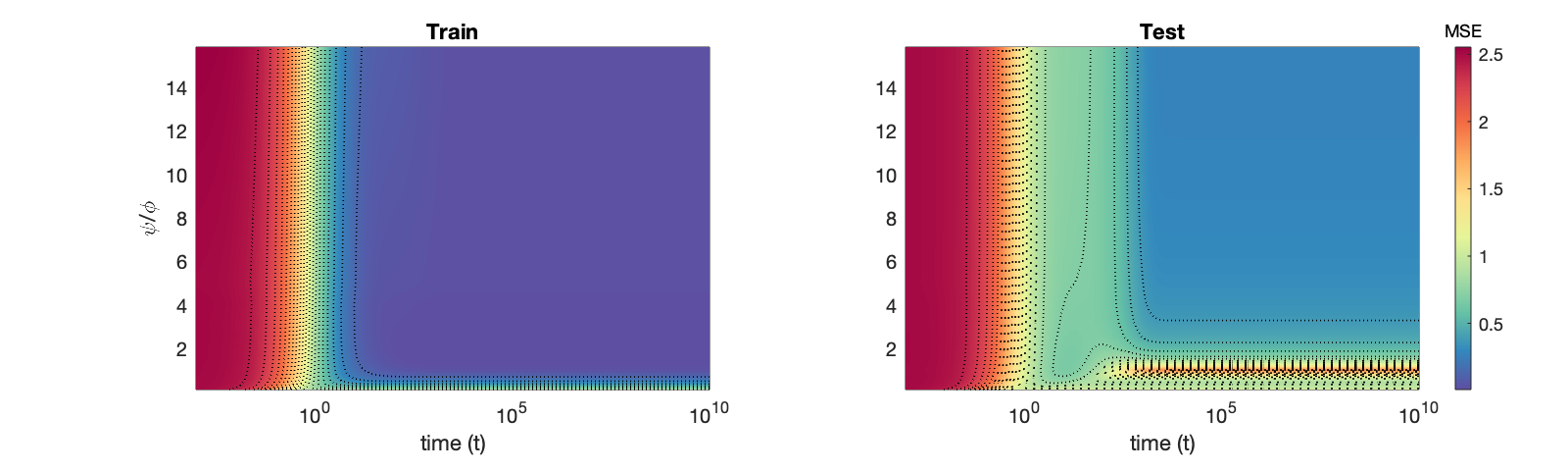
Figure 6: Analytical training error and test error evolution at fixed $\delta$ with parameters $(\mu,\nu,\phi,r,s,\delta)=(0.5,0.3,3,2.,0.4,0.001)$

Figure 7: Analytical training error and test error evolution with parameters $(\mu,\nu,\phi,r,s,\lambda)=(0.5,0.3,3,0,0.4,0.001)$

Figure 8: Analytical training error and test error evolution with parameters $(\mu,\nu,\phi,r,s,\lambda)=(0.5,0.3,0.5,2,0.1,0.003)$

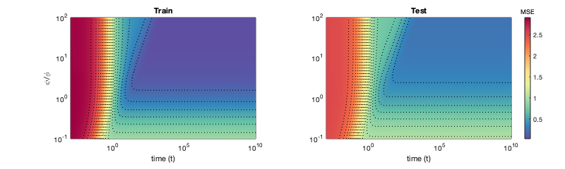
Figure 9: Analytical training error and test error evolution with parameters $(\mu,\nu,\phi,r,s,\lambda)=(0.5,0.3,3,0,0.4,0.1)$

Figure 10: Analytical training error and test error evolution with parameters corresponding to $\sigma(x)=\tanh(x)$ with $(\mu,\nu,\phi,r,s,\lambda)=(0.61,0.15,3,0,0.4,0.001)$

Figure 11: Analytical training error and test error evolution with parameters corresponding to $\sigma(x)=\tanh(5x)$ with $(\mu,\nu,\phi,r,s,\lambda)=(0.79,0.47,3,2,0.4,0.001)$

Figure 12: Analytical training error with parameters $(\mu,\nu,\phi,r,s,\lambda)=(0.5,0.3,3,2.,0.4,0.001)$

F.4 Comparison with experimental simulations

We have already shown on figure 2 in Sect. 3 that the analytical formulas for the training and generalization errors match the experimental curves in the limit of $t\to+\infty$. Here we provide additional evidence that this is also the case for the whole time-evolution in Figs. 13 and 14 as the dimension $d$ increases.

In 15, 16, we can see that the epoch-wise descent structures of the training error and test error can be captured correctly experimentally for long time. Note that we have taken $d=100$ small enough to be able to run these experiments for such a long timescale.

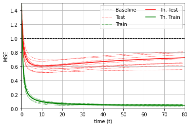
(a)

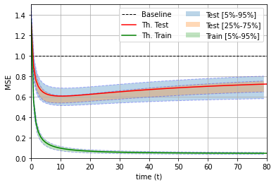
(b)

Figure 13: Analytical training error and test error profile with parameters $(\mu,\nu,\phi,\psi,r,s,\lambda)=(0.5,0.3014,1.4,1.8,1.0,0,0.01)$ compared to 10 experimental runs ($\sigma=\text{Relu}-\frac{1}{\sqrt{2\pi}}$) with $d=200$ and $\mathrm{d}t=0.01$

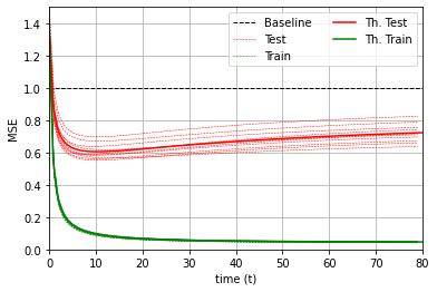
(a)

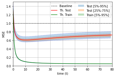
(b)

Figure 14: Analytical training error and test error profile with parameters $(\mu,\nu,\phi,\psi,r,s,\lambda)=(0.5,0.3014,1.4,1.8,1.0,0,0.01)$ compared to 10 experimental runs ($\sigma=\text{Relu}-\frac{1}{\sqrt{2\pi}}$) with $d=1000$ and $\mathrm{d}t=0.01$

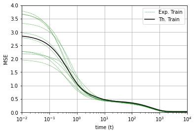
Figure 15: Analytical training error with parameters $(\mu,\nu,\phi,\psi,r,s,\lambda)=(0.5,0.3,300,3,2,0.4,0.1)$ compared to 10 experimental runs ($\sigma=\text{Relu}-\frac{1}{\sqrt{2\pi}}$) with $d=100$ and $\mathrm{d}t=0.01$

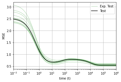
Figure 16: Analytical test error with parameters $(\mu,\nu,\phi,\psi,r,s,\lambda)=(0.5,0.3,6,3,2,0.4,0.0001)$ compared to 10 experimental runs with $d=100$ and $\mathrm{d}t=0.01$ for $0\leq t\leq 10^{4}$ and $\mathrm{d}t=0.1$ for $10^{4}\leq t\leq 10^{6}$

References

- [1] Tom Brown, Benjamin Mann, Nick Ryder, Melanie Subbiah, Jared D Kaplan, Prafulla Dhariwal, Arvind Neelakantan, Pranav Shyam, Girish Sastry, Amanda Askell, Sandhini Agarwal, Ariel Herbert-Voss, Gretchen Krueger, Tom Henighan, Rewon Child, Aditya Ramesh, Daniel Ziegler, Jeffrey Wu, Clemens Winter, Chris Hesse, Mark Chen, Eric Sigler, Mateusz Litwin, Scott Gray, Benjamin Chess, Jack Clark, Christopher Berner, Sam McCandlish, Alec Radford, Ilya Sutskever, and Dario Amodei. Language models are few-shot learners. In H. Larochelle, M. Ranzato, R. Hadsell, M. F. Balcan, and H. Lin, editors, Advances in Neural Information Processing Systems, volume 33, pages 1877–1901. Curran Associates, Inc., 2020.
- [2] Jared Kaplan, Sam McCandlish, Tom Henighan, Tom B. Brown, Benjamin Chess, Rewon Child, Scott Gray, Alec Radford, Jeffrey Wu, and Dario Amodei. Scaling laws for neural language models. arXiv, page 2001.08361v1, 2020.
- [3] Trevor Hastie, Robert Tibshirani, and Jerome Friedman. The Elements of Statistical Learning. Springer Series in Statistics. Springer New York Inc., New York, NY, USA, 2001.
- [4] Chiyuan Zhang, Samy Bengio, Moritz Hardt, Benjamin Recht, and Oriol Vinyals. Understanding deep learning requires rethinking generalization. ICLR 2017, arXiv abs/1611.03530, 2016.
- [5] Mikhail Belkin, Daniel Hsu, Siyuan Ma, and Soumik Mandal. Reconciling modern machine-learning practice and the classical bias-variance trade-off. Proceedings of the National Academy of Sciences, 116:201903070, 07 2019.
- [6] Mikhail Belkin, Siyuan Ma, and Soumik Mandal. To understand deep learning we need to understand kernel learning. In Jennifer Dy and Andreas Krause, editors, Proceedings of the 35th International Conference on Machine Learning, volume 80 of Proceedings of Machine Learning Research, pages 541–549. PMLR, 10–15 Jul 2018.
- [7] Mikhail Belkin, Alexander Rakhlin, and Alexandre B. Tsybakov. Does data interpolation contradict statistical optimality? In Kamalika Chaudhuri and Masashi Sugiyama, editors, Proceedings of the Twenty-Second International Conference on Artificial Intelligence and Statistics, volume 89 of Proceedings of Machine Learning Research, pages 1611–1619. PMLR, 16–18 Apr 2019.
- [8] Mikhail Belkin, Daniel Hsu, and Ji Xu. Two models of double descent for weak features. SIAM Journal on Mathematics of Data Science, 2(4):1167–1180, Jan 2020.
- [9] S Spigler, M Geiger, S d’Ascoli, L Sagun, G Biroli, and M Wyart. A jamming transition from under- to over-parametrization affects generalization in deep learning. Journal of Physics A: Mathematical and Theoretical, 52(47):474001, Oct 2019.
- [10] Mario Geiger, Arthur Jacot, Stefano Spigler, Franck Gabriel, Levent Sagun, Stéphane d’Ascoli, Giulio Biroli, Clément Hongler, and Matthieu Wyart. Scaling description of generalization with number of parameters in deep learning. Journal of Statistical Mechanics: Theory and Experiment, 2020(2):023401, feb 2020.
- [11] Madhu S. Advani, Andrew M. Saxe, and Haim Sompolinsky. High-dimensional dynamics of generalization error in neural networks. Neural Networks, 132:428–446, 2020.
- [12] Trevor Hastie, Andrea Montanari, Saharon Rosset, and Ryan J. Tibshirani. Surprises in High-Dimensional Ridgeless Least Squares Interpolation. arXiv e-prints, page arXiv:1903.08560, March 2019.
- [13] Michal Derezinski, Feynman T Liang, and Michael W Mahoney. Exact expressions for double descent and implicit regularization via surrogate random design. In H. Larochelle, M. Ranzato, R. Hadsell, M. F. Balcan, and H. Lin, editors, Advances in Neural Information Processing Systems, volume 33, pages 5152–5164. Curran Associates, Inc., 2020.
- [14] Vidya Muthukumar, Kailas Vodrahalli, Vignesh Subramanian, and Anant Sahai. Harmless interpolation of noisy data in regression. IEEE Journal on Selected Areas in Information Theory, 1(1):67–83, 2020.
- [15] Peter L. Bartlett, Philip M. Long, Gábor Lugosi, and Alexander Tsigler. Benign overfitting in linear regression. Proceedings of the National Academy of Sciences, 117(48):30063–30070, 2020.
- [16] Zeyu Deng, Abla Kammoun, and Christos Thrampoulidis. A model of double descent for high-dimensional binary linear classification. Information and Inference: A Journal of the IMA, 04 2021. iaab002.
- [17] Song Mei and Andrea Montanari. The generalization error of random features regression: Precise asymptotics and double descent curve. arXiv e-prints, page arXiv:1908.05355, August 2019.
- [18] Zhenyu Liao, Romain Couillet, and Michael W Mahoney. A random matrix analysis of random Fourier features: beyond the Gaussian kernel, a precise phase transition, and the corresponding double descent. In 34th Conference on Neural Information Processing Systems (NeurIPS 2020), Vancouver, Canada, December 2020.
- [19] Federica Gerace, Bruno Loureiro, Florent Krzakala, Marc Mezard, and Lenka Zdeborova. Generalisation error in learning with random features and the hidden manifold model. In Hal Daumé III and Aarti Singh, editors, Proceedings of the 37th International Conference on Machine Learning, volume 119 of Proceedings of Machine Learning Research, pages 3452–3462. PMLR, 13–18 Jul 2020.
- [20] Stéphane D’Ascoli, Maria Refinetti, Giulio Biroli, and Florent Krzakala. Double trouble in double descent: Bias and variance(s) in the lazy regime. In Hal Daumé III and Aarti Singh, editors, Proceedings of the 37th International Conference on Machine Learning, volume 119 of Proceedings of Machine Learning Research, pages 2280–2290. PMLR, 13–18 Jul 2020.
- [21] Stéphane d’Ascoli, Levent Sagun, and Giulio Biroli. Triple descent and the two kinds of overfitting: where and why do they appear? In H. Larochelle, M. Ranzato, R. Hadsell, M. F. Balcan, and H. Lin, editors, Advances in Neural Information Processing Systems, volume 33, pages 3058–3069. Curran Associates, Inc., 2020.
- [22] Preetum Nakkiran, Gal Kaplun, Yamini Bansal, Tristan Yang, Boaz Barak, and Ilya Sutskever. Deep double descent: Where bigger models and more data hurt. In International Conference on Learning Representations, 2020.
- [23] Manfred Opper. Statistical Mechanics of Generalization, pages 922–925. MIT Press, Cambridge, MA, USA, 1998.
- [24] A. Engel and C. Van den Broeck. Statistical Mechanics of Learning. Cambridge University Press, 2001.
- [25] Ali Rahimi and Benjamin Recht. Random features for large-scale kernel machines. In J. Platt, D. Koller, Y. Singer, and S. Roweis, editors, Advances in Neural Information Processing Systems, volume 20. Curran Associates, Inc., 2008.
- [26] Arthur Jacot, Berfin Simsek, Francesco Spadaro, Clement Hongler, and Franck Gabriel. Implicit regularization of random feature models. In Hal Daumé III and Aarti Singh, editors, Proceedings of the 37th International Conference on Machine Learning, volume 119 of Proceedings of Machine Learning Research, pages 4631–4640. PMLR, 13–18 Jul 2020.
- [27] Antoine Bodin and Nicolas Macris. Rank-one matrix estimation: analytic time evolution of gradient descent dynamics. In Mikhail Belkin and Samory Kpotufe, editors, Proceedings of Thirty Fourth Conference on Learning Theory, volume 134 of Proceedings of Machine Learning Research, pages 635–678. PMLR, 15–19 Aug 2021.
- [28] Zhenyu Liao and Romain Couillet. The dynamics of learning: A random matrix approach. In International Conference on Machine Learning, pages 3072–3081. PMLR, 2018.
- [29] Ben Adlam and Jeffrey Pennington. The neural tangent kernel in high dimensions: Triple descent and a multi-scale theory of generalization. In Hal Daume III and Aarti Singh, editors, Proceedings of the 37th International Conference on Machine Learning, volume 119 of Proceedings of Machine Learning Research, pages 74–84. PMLR, 13–18 Jul 2020.
- [30] Reza Rashidi Far, Tamer Oraby, Wlodzimierz Bryc, and Roland Speicher. Spectra of large block matrices. arXiv e-prints, page cs/0610045, October 2006.
- [31] J. W. Helton, R. R. Far, and R. Speicher. Operator-valued semicircular elements: Solving a quadratic matrix equation with positivity constraints. International Mathematics Research Notices, 2007(9):rnm086–rnm086, 2007.
- [32] J William Helton, Tobias Mai, and Roland Speicher. Applications of realizations (aka linearizations) to free probability. Journal of Functional Analysis, 274(1):1–79, 2018.
- [33] Jeffrey Pennington and Pratik Worah. Nonlinear random matrix theory for deep learning. In Isabelle Guyon, Ulrike von Luxburg, Samy Bengio, Hanna M. Wallach, Rob Fergus, S. V. N. Vishwanathan, and Roman Garnett, editors, Advances in Neural Information Processing Systems 30: Annual Conference on Neural Information Processing Systems 2017, December 4-9, 2017, Long Beach, CA, USA, pages 2637–2646, 2017.
- [34] S. Péché. A note on the Pennington-Worah distribution. Electronic Communications in Probability, 24(none):1 – 7, 2019.
- [35] David A. Cox, John Little, and Donal O’Shea. Ideals, Varieties, and Algorithms: An Introduction to Computational Algebraic Geometry and Commutative Algebra, 3/e (Undergraduate Texts in Mathematics). Springer-Verlag, Berlin, Heidelberg, 2007.
- [36] Alethea Power, Yuri Burda, Harri Edwards, Igor Babuschkin, and Vedant Misra. Grokking: Generalization beyond overfitting on small algorithmic datasets. In ICLR MATH-AI Workshop, 2021.
- [37] Ben Adlam, Jake Levinson, and Jeffrey Pennington. A Random Matrix Perspective on Mixtures of Nonlinearities for Deep Learning. arXiv e-prints, page arXiv:1912.00827, December 2019.
- [38] James A Mingo and Roland Speicher. Free probability and random matrices, volume 35. Springer, 2017.
- [39] Samuel F Edwards and Raymund C Jones. The eigenvalue spectrum of a large symmetric random matrix. Journal of Physics A: Mathematical and General, 9(10):1595, 1976.
- [40] Bruno Loureiro, Cédric Gerbelot, Hugo Cui, Sebastian Goldt, Florent Krzakala, Marc Mézard, and Lenka Zdeborová. Capturing the learning curves of generic features maps for realistic data sets with a teacher-student model. arXiv preprint arXiv:2102.08127, 2021.
- [41] G. Parisi, P. Urbani, and F. Zamponi. Theory of Simple Glasses: Exact Solutions in Infinite Dimensions. Cambridge University Press, 2020.
- [42] H. Sompolinsky, A. Crisanti, and H. J. Sommers. Chaos in random neural networks. Phys. Rev. Lett., 61:259–262, Jul 1988.
- [43] A. Crisanti and H. Sompolinsky. Path integral approach to random neural networks. Phys. Rev. E, 98:062120, Dec 2018.
- [44] Elisabeth Agoritsas, Giulio Biroli, Pierfrancesco Urbani, and Francesco Zamponi. Out-of-equilibrium dynamical mean-field equations for the perceptron model. Journal of Physics A: Mathematical and Theoretical, 51(8):085002, Jan 2018.
- [45] Francesca Mignacco, Florent Krzakala, Pierfrancesco Urbani, and Lenka Zdeborová. Dynamical mean-field theory for stochastic gradient descent in gaussian mixture classification. In H. Larochelle, M. Ranzato, R. Hadsell, M. F. Balcan, and H. Lin, editors, Advances in Neural Information Processing Systems, volume 33, pages 9540–9550. Curran Associates, Inc., 2020.
- [46] Francesca Mignacco, Pierfrancesco Urbani, and Lenka Zdeborová. Stochasticity helps to navigate rough landscapes: comparing gradient-descent-based algorithms in the phase retrieval problem. Machine Learning: Science and Technology, 2021.