Resolution-vs.-Accuracy Dilemma in Machine Learning Modeling of Electronic Excitation Spectra

Abstract

In this study, we explore the potential of machine learning for modeling molecular electronic spectral intensities as a continuous function in a given wavelength range. Since presently available chemical space datasets provide excitation energies and corresponding oscillator strengths for only a few valence transitions, here, we present a new dataset—bigQM7$\rm{\omega}$ —with 12,880 molecules containing up to 7 CONF atoms and report ground state and excited state properties. A publicly accessible web-based data-mining platform is presented to facilitate on-the-fly screening of several molecular properties including harmonic vibrational and electronic spectra. We present all singlet electronic transitions from the ground state calculated using the time-dependent density functional theory framework with the $\omega$B97XD exchange-correlation functional and a diffuse-function augmented basis set. The resulting spectra predominantly span the X-ray to deep-UV region (10–120 nm). To compare the target spectra with predictions based on small basis sets, we bin spectral intensities and show good agreement is obtained only at the expense of the resolution. Compared to this, machine learning models with latest structural representations trained directly using $<10\%$ of the target data recover the spectra of the remaining molecules with better accuracies at a desirable $<1$ nm wavelength resolution.

I Introduction

The future of chemistry research hinges on the progress in data-driven autonomous discoveriesSteiner et al. (2019); Christensen et al. (2021); Stach et al. (2021). The performance of intelligent infrastructures necessary for such endeavors, such as chemputersGromski et al. (2020), can be tremendously enhanced when augmenting experimental data used for their training with accurate ab initio resultsLi et al. (2021); Bai et al. (2019). For designing opto-electronically important molecules such as dye-sensitized solar cellsMathew et al. (2014); Abreha et al. (2019), sunscreensSampedro (2011); Losantos et al. (2017), or organic photovoltaicsHachmann et al. (2011); Pyzer-Knapp et al. (2015), the corresponding target properties are excitation energies and the associated spectral intensities. Additionally, successful molecular design also requires information about thermodynamic/dynamic/kinetic stabilities, molecular lifetimes, solubility, and other experimental factors pertaining to molecular characterization. Accelerated discoveries based on molecular design workflows require a seamless supply of accurate theoretical results. To this end, machine learning (ML) models trained on results from ab initio predictions have emerged as their rapid and accurate surrogatesRupp et al. (2012); Ramakrishnan and von Lilienfeld (2017); von Lilienfeld (2018).

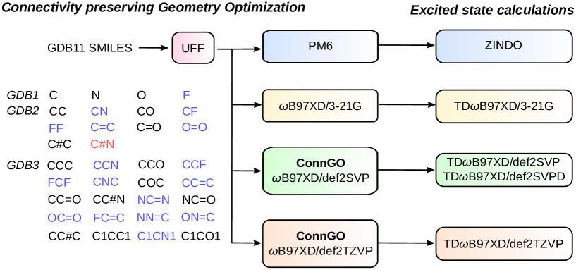
Figure 1: bigQM7$\rm{\omega}$ chemical space design: Molecular composition and data generation workflows. From the GDB11 dataset, SMILES descriptors for all molecules with up to 7 CONF atoms were collected. For the GDB1-GDB3 subsets, CHONF molecules present in GDB11 but absent in GDB17 are shown in blue. HCN that is present in GDB17, but absent in GDB11 is shown in red. Initial geometries were obtained with UFF that are subsequently optimized at the PM7 and $\omega$B97XD/3-21G levels. $\omega$B97XD geometry optimizations with large basis sets (def2SVP and def2TZVP) were done using the ConnGO workflow. TDDFT single point calculations were done using the DFT equilibrium geometries, while ZINDO calculations were done at PM6 geometries.

ML models have been shown to accurately forecast a multitude of globalRupp et al. (2012); Ramakrishnan and von Lilienfeld (2015); Ramakrishnan et al. (2015a) and quasi-atomic molecular propertiesRupp et al. (2015); Gerrard et al. (2020); Gupta et al. (2021). For atomization or bonding energies, their prediction uncertainties are comparable to that of hybrid density functional theory (DFT) approximationsHansen et al. (2015); Ramakrishnan and von Lilienfeld (2017); Faber et al. (2018); Qiao et al. (2020); Unke and Meuwly (2019); Schütt et al. (2017); Faber et al. (2017). They have also successfully modeled non-adiabatic molecular dynamicsPrezhdo (2021), vibrational spectraLam et al. (2020); Kananenka et al. (2019), electronic coupling elementsÇaylak et al. (2019), excitonsVela et al. (2021), electronic densitiesGrisafi et al. (2018), excited states in diverse chemical spacesRamakrishnan et al. (2015b); Tapavicza et al. (2021); Çaylak and Baumeier (2021), as well as excited-state potential energy surfaces (PES)Westermayr and Marquetand (2020a, b); Tapavicza et al. (2021); Dral and Barbatti (2021); Rankine and Penfold (2021). A key difference in the performance of ML in the latter two application domains is that ambiguities due to atomic indices and size-extensivity that affect the quality of structural representations for chemical space explorationsHansen et al. (2013); von Lilienfeld et al. (2015) do not arise in PES modeling or dipole surface modelingHuang et al. (2005); Behler (2015); Manzhos and Carrington Jr (2020) resulting in better learning rates.

ML models of global molecular energies (atomization/formation energies, etc.) with a robust structural representation benefit from the well-known mapping between the ground state electronic energy and the corresponding minimum energy geometry established by the Hohenberg–Kohn theoremHohenberg and Kohn (1964). The Runge–Gross theorem provides a similar mapping between the time-dependent potential and the time-evolved total electron densityRunge and Gross (1984). However, the target quantities in ML modeling of excited states are state-specific stemming from local molecular regions. For quasi-atomic properties such as ¹³C NMR shielding constantsRupp et al. (2015); Gerrard et al. (2020); Gupta et al. (2021); Rankine and Penfold (2021) or K-edge X-ray absorption spectroscopyRupp et al. (2015); Rankine and Penfold (2021), a representation encoding the local environment of the query atom results in better learning rates. Similarly, quasi-particle density-of-states—interpreted as intensities in a photo-emission spectrum—have also been successfully modeledMahmoud et al. (2020); Westermayr and Maurer (2021). However, for valence electronic excitations that are also local, the corresponding molecular substructure varies non-trivially across the chemical space. Hence, intensities based on oscillator strengths derived from many-electron excited state wave functions obeying dipole selection rules exhibit slow learning ratesTapavicza et al. (2021). Determining the characteristic chromophore responsible for the electronic excitations is non-trivial for chemical space datasets such as QM9Ramakrishnan et al. (2014) that exhibit large structural diversity. This complexity, in turn, hinders the development of local descriptors that can map to the composition or structure of the chromophore and its environment. Hence, we are limited to using global structural representations for ML modeling of electronic excited state properties. This limitation becomes evident from the modest performances of ML models of excitation energiesRamakrishnan et al. (2015b); Tapavicza et al. (2021), and their zero-order approximations, the frontier molecular orbital (MO) energiesFaber et al. (2018); Liu et al. (2021); Mazouin et al. (2021); Çaylak and Baumeier (2021).

Table 1: Comparison of volume, variety and veracity of selected small molecules chemical space datasets. Size, composition and methods (only DFT or post-DFT) used for data generation are listed.

Details	QM7	QM7b	QM9a	bigQM7$\rm{\omega}$
Origin	GDB13	GDB13	GDB17	GDB11
Elements	CHONS	CHONSCl	CHONF	CHONF
Size	7165	7211	133885	12880
Geometry optimization	PBE0/tight tier-2	PBE/tight tier-2	B3LYP/6-31G(2df,p)	$\omega$B97XD/3-21G
				$\omega$B97XD/def2SVP
				$\omega$B97XD/def2TZVP
Frequencies			B3LYP/6-31G(2df,p)	$\omega$B97XD/3-21G
				$\omega$B97XD/def2SVP
				$\omega$B97XD/def2TZVP
Excited states		$E_{1}$	$E_{1}$, $E_{2}$, $f_{1}$, $f_{2}$	all states
		GW/tight tier-2	RICC2/def2TZVP	TD$\omega$B97XD/3-21G
			TDPBE0/def2SVP	TD$\omega$B97XD/def2SVP
			TDPBE0/def2TZVP	TD$\omega$B97XD/def2TZVP
			TDCAMB3LYP/def2TZVP	TD$\omega$B97XD/def2SVPD

• Contains 3993/22786 molecules with up to 7/ 8 CONF atoms. Excited state data are available for the 22786 subset Ref.33.

In this study, we: (i) Present a high-quality chemical space dataset, bigQM7$\rm{\omega}$ , containing ground-state properties and electronic spectra of 12,880 molecules containing up to 7 CONF atoms modeled at the $\omega$B97XD level with different basis sets. (ii) Demonstrate the resolution-vs-accuracy dilemma in modeling spectroscopic intensities. (iii) Present ML models trained on the bigQM7$\rm{\omega}$ dataset for an accurate reconstruction of the electronic spectra of allowed transitions in a given wavelength domain.

II Chemical Space Design

II.1 The bigQM7$\rm{\omega}$ dataset

Pioneering efforts in small molecular chemical space design have culminated in the graph-based generated dataset, GDB11Fink et al. (2005); Fink and Reymond (2007), containing 0.9 billion molecules with up to 11 CONF atoms. GDB11 provides simplified-molecular-input-line-entry-system (SMILES) string-based descriptors encoding molecular graphs. Larger datasets, GDB13Blum and Reymond (2009) and GDB17Ruddigkeit et al. (2012) have since been created containing 13 and 17 heavy atoms, respectively. Synthetic feasibility and drug-likeness criteria eliminated several molecules in GDB13 and GDB17. Starting with the SMILES descriptors of GDB13, QM7Rupp et al. (2012) and QM7bMontavon et al. (2013) quantum chemistry datasets emerged, provisioning computed equilibrium geometries and several molecular properties. Recently, QM7 has been extended by including non-equilibrium geometries for each molecule resulting in QM7-XHoja et al. (2021). Similarly, the QM9 datasetRamakrishnan et al. (2014) used SMILES from the GDB17 library reporting structures and properties of 134k molecules with up to 9 CONF atoms.

In the present work, we explore molecules with up to 7 CONF atoms. We begin with the GDB11 set of SMILES because several important molecules such as ethylene and acetic acid present in GDB11 were filtered out in GDB13 and GDB17. Our new dataset contains 12883 molecules—almost twice as large as the QM7 sets. The breakdown for subsets with 1/2/3/4/5/6/7 heavy atoms is 4/9/20/80/352/1850/10568. The previous datasets QM7, QM7b, and QM9 have been generated using yesteryear’s quantum chemistry workhorses: PBEPerdew et al. (1996), PBE0Adamo and Barone (1999), and B3LYPBecke (1993). Here, we use the range-separated hybrid DFT method, $\omega$B97XDChai and Head-Gordon (2008) that is gaining widespread popularity for its excellent accuracy. Hence, we name this dataset as bigQM7$\rm{\omega}$ , with the last character emphasizing the DFT approximation utilized. The high-throughput workflow used for generating bigQM7$\rm{\omega}$ is shown in Fig. 1 and Table 1 puts the new dataset in perspective by comparing with other popular datasets of similar constitution. While bigQM7$\rm{\omega}$ is smaller than QM9, it provides a better coverage of molecules for the same number of CONF atoms. Further, bigQM7$\rm{\omega}$ also provides excited state data collected at various theoretical levels, hence, comprehensively covering the property domain. A summary of properties of bigQM7$\rm{\omega}$ , made available in the form of structured datasetsKayastha and Ramakrishnan (2021a), is provided in Table 2. As unstructured datasets, we provide raw input/output filesKayastha and Ramakrishnan (2021b) to kindle future endeavors. For example, for ML modeling of forces, properties of non-equilibrium geometries may be extracted from these raw data.

Table 2: Structured content of the bigQM7$\rm{\omega}$ datasetKayastha and Ramakrishnan (2021a).

PM6

Equilibrium geometries (Å)

All molecular orbital energies (hartree)

Total electronic and atomization energies (hartree)

$\omega$B97XD/(3-21G, def2SVP, def2TZVP)

Equilibrium geometries (Å)

All molecular orbital energies (hartree)

Atomization energies (hartree)

All harmonic frequencies (cm-1)

Zero-point vibrational energy (kcal/mol)

Mulliken charges, atomic polar tensor charges ($e$)

Dipole moment (debye)

Polarizability (bohr3)

Radial expectation value (bohr2)

Internal energy at 0 K and 298.15 K (hartree)

Enthalpy at 298.15 K (hartree)

Free energy at 298.15 K (hartree)

Total heat capacity (Cal/mol/K)

ZINDO, TD$\omega$B97XD/(3-21G, def2SVP, def2TZVP, def2SVPD)

Excitation energy of all states (eV, nm)

Oscillator strengths of all excitations (dimensionless)

Transition dipole moment of all excitations (au)

II.2 Computational Details

Initial structures of the 12883 molecules in bigQM7$\rm{\omega}$ were generated from SMILES by relaxing with the universal force field (UFF)Rappé et al. (1992) employing tight convergence criteria using OpenBabelO’Boyle et al. (2011). As a guideline for quantum chemistry big data generation, a previous study proposed connectivity preserving geometry optimizations (ConnGO) to eliminate structural ambiguities due to rearrangements encountered in automated high-throughput calculationsSenthil et al. (2021). Accordingly, we used a 3-tier ConnGO workflow to generate geometries at the $\omega$B97XDChai and Head-Gordon (2008) DFT level using def2SVP and def2TZVP basis setsWeigend and Ahlrichs (2005). Geometry optimizations at the simpler levels such as PM6 and $\omega$B97XD/3-21G were performed without ConnGO, directly starting from the UFF structures. For $\omega$B97XD/def2SVP final geometries, we used HF/STO3G and $\omega$B97XD/3-21G as intermediate tier-1 and tier-2 levels, respectively. Similarly, for $\omega$B97XD/def2TZVP, HF/STO3G and $\omega$B97XD/def2SVP were lower tiers. In each tier, ConnGO compares the optimized geometry with the covalent bonding connectivities encoded in the initial SMILES and detects molecules undergoing rearrangements. For this purpose, we used the ConnGO thresholds: 0.2 Å for the maximum absolute deviation in covalent bond length and a mean percentage absolute deviation of 6%. In DFT calculations, tight optimization thresholds and ultrafine grids were used for evaluating the exchange-correlation (XC) energy. A few molecules required relaxing the optimization thresholds for monotonic convergence towards a minimum. All final geometries were confirmed to be local minima through harmonic frequency analysis. For molecules that are highly symmetric or with multiple triple bonds, converging to minima was only possible with the verytight optimization threshold and superfine grids. At both $\omega$B97XD/def2SVP and $\omega$B97XD/def2TZVP levels, 3 molecules with the SMILES O=c1cconn1, N=c1nconn1, O=c1nconn1, failed the ConnGO connectivity tests. Further investigation revealed these molecules to contain an -NNO- substructure in a 6-membered ring facilitating dissociation as previously noted in  Ref.66. After removing these molecules, the size of bigQM7$\rm{\omega}$ stands at 12880.

We performed vertical excited-state calculations at Zerner’s intermediate neglect of differential overlap (ZINDO)Ridley and Zerner (1973) and TD$\omega$B97XD levels. ZINDO calculations were done on PM6 minimum energy geometries, while TD$\omega$B97XD with 3-21G, def2SVP, and def2TZVP basis sets, at the corresponding ground state equilibrium geometries. We also performed TD$\omega$B97XD calculations with the diffuse function augmented basis set, def2SVPD, on $\omega$B97XD/def2SVP geometries. All electronic structure calculations were performed using the Gaussian suite of programsFrisch et al. (2016). The number of excited states accessible to the TDDFT formalism is limited by the number of electrons and the size of the orbital basis set. With the finite basis set used in this study, the spectrum is practically discrete. To ensure that all the singlet-type electronic bound states are calculated, we set an upper bound of 10,000 for the number of states in the TDDFT single point calculations with the keyword nstates=10000. For benchmarking the quality of TDDFT excitation spectra, we also performed similarity transformed equation-of-motion coupled cluster with singles doubles excitation (STEOM-CCSD)Nooijen and Bartlett (1997) and the aug-cc-pVTZ basis set as implemented in OrcaNeese (2012, 2018).

III Machine Learning Modeling of Full Electronic Spectra

Kernel ridge regression (KRR) based ML (KRR-ML) enables accurate predictions through an exact global optimization of a convex modelSchölkopf et al. (2002); Rupp et al. (2012); Ramakrishnan and von Lilienfeld (2017). In KRR-ML the target property, $t_{q}$, of an out-of-sample query, $q$, is estimated as the linear combination of kernel (or radial basis) functions, each centered on a training entry. Formally, with a suitable choice of the kernel function, KRR approaches the target when the training set is sufficiently large

$$t_{q}=\lim_{N\rightarrow\infty}\sum_{i=1}^{N}c_{i}k({\bf d}_{q}-{\bf d}_{i}).$$ (1)

The coefficients, $\{c_{i}\}$, are obtained by regression over the training data. The kernel function, $k(\cdot)$, captures the similarity in the representations of the query, $q$, and all $N$ training examples. For ground state energetics, the Faber-Christensen-Huang-Lilienfeld (FCHL) formalism in combination with KRR-ML has been shown to perform better than other structure-based representationsFaber et al. (2018); Christensen et al. (2020). However, for excitation energies and frontier MO gaps, FCHL’s performance drops compared to the spectral London-Axilrod-Teller-Muto (SLATM) representationHuang and von Lilienfeld (2020). In this study, we compare the performance of FCHL and SLATM for modeling the full-electronic spectrum. SLATM delivers best accuracies with the Laplacian kernel, $k(\textbf{d}_{q},\textbf{d}_{i})=\exp(-|\textbf{d}_{q}-\textbf{d}_{i}|_{1}/\sigma)$, where $\sigma$ defines the length scale of the kernel function and $|\cdot|_{1}$ denotes $L_{1}$ norm. For the FCHL formalism, we found an optimal kernel width of $\sigma=5$ through scanning and a cutoff distance of 20 Å was used to sufficiently capture the structural features of the longest molecule in the bigQM7$\rm{\omega}$ dataset, heptane.

The kernel width, $\sigma$, is traditionally determined through cross-validation. For multi-property modeling $\sigma$ can be estimated using the ‘single-kernel’ approachRamakrishnan and von Lilienfeld (2015), where $\sigma$ is estimated as a function of the largest descriptor difference in a sample of the training set, $\sigma={\rm max}\{d_{ij}\}/{\rm log}(2)$. Previous worksRamakrishnan and von Lilienfeld (2015); Gupta et al. (2021); Kayastha and Ramakrishnan (2021c) have shown single-kernel modeling to agree with cross-validated results with in the uncertainty arising due to training set shuffles, especially for large training set sizes. KRR with a single-kernel facilitates seamless modeling of multiple molecular properties using standard linear solvers

$$[{\bf K}+\zeta{\bf I}][{\bf c}_{1},{\bf c}_{2},\ldots]=[{\bf p}_{1},{\bf p}_{2},\ldots],$$ (2)

where ${\bf p}_{j}$ is $j$-th property vector and ${\bf c}_{j}$ is the corresponding regression coefficient vector. We use Cholesky decomposition that offers the best scaling of $2N^{3}/6$ for dense kernel matrices of size $N$Van Loan and Golub (1996). The diagonal elements of the kernel matrix are shifted by a positive hyperparameter, $\zeta$ to regularize the fit, i.e., prevent over-fitting. We note in passing that conventionally the regularization strength is denoted by the symbol $\lambda$, which we reserve in this study for wavelength. Another role of $\zeta$ is to make the kernel matrix positive definite if there is linear dependency in the feature space arising either due to redundant training entries or due to poor choice of representations. Even though we have ensured that our dataset is devoid of redundant entries, and the representations used here accurately map to the molecular structure, we cannot a priori rule out weak linear dependencies arising from numerical reasons. Hence, we condition the kernel matrix by setting $\zeta$ to a small value of $10^{-4}$. We generated SLATM representation vectors and the FCHL kernel using the QML codeChristensen et al. (2017), and performed all other ML calculations using in-house programs written in Fortran. All ML errors reported in this study are based on 20 shuffles of the data to prevent selection bias for small training set sizes. In all learning curves the error bars due to shuffles are vanishingly small for large training set sizes, hence the corresponding envelopes are not shown. Further, both SLATM and FCHL models were generated using geometries relaxed using UFF in order for the out-of-sample querying to be rapid.

The property (${\bf p}_{i}$ vector in Eq. 2) modeled in this study corresponds to sum of binned oscillator strength of electronic transitions from the ground state. Conventionally, the band intensity due to the $k-$th excitation is the molar absorption coefficient that is proportional to the corresponding oscillator strength, $f_{0\rightarrow k}$, denoted shortly as $f_{k}$Turro et al. (2017). In order to model a full spectrum in a given wavelength range, one can consider each value of $f_{k}$ (in atomic units, a.u.) as a separate target quantity. However, the number of states is not uniform in a dataset such as bigQM7$\rm{\omega}$ . Further, in practice, one is interested in an integrated oscillator strengths within a small resolution, $\Delta\lambda$. Hence, we uniformly divide the spectral range in powers of 2, $\Delta\lambda=\lambda_{\rm spectrum}/N_{\rm bin}$, where $N_{\rm bin}=1,2,4,\ldots$ is the number of bins. For the small organic molecules such as those in bigQM7$\rm{\omega}$ , we set spectral range to $\lambda_{\rm spectrum}$ to 120 nm capturing most of the excitations. For wavelengths $>120$ nm the bigQM7$\rm{\omega}$ dataset provides too few examples, hence, data in this long wavelength domain is inadequate for ML modeling. The target for ML is the sum of $f_{k}$ in a bin

$$p_{i}(\lambda_{i})=\sum_{k=1}^{\rm all\,states}f_{k}(\lambda_{k}),$$ (3)

where $i$ is the bin index, and $\lambda_{i}$ is the central wavelength of the bin. The oscillator strength of $k$-th excitation from the ground state falls in the $i$-th bin if $\lambda_{k}\in\left(\lambda_{i}-\Delta\lambda/2,\lambda_{i}+\Delta\lambda/2\right]$. Since we consider $f_{k}$ in a.u., $p_{i}$ are also in the same units. We explore the performance of ML models for various number of bins. For the limiting case, $\Delta\lambda=\lambda_{\rm spectrum}$, the target property is the sum of oscillator strengths of all excitations in the selected spectral range, i.e., all the intensities are in one bin. The maximum number of bins explored is 128, which results in a spectral resolution of 0.94 nm (=120/128). In this case, Cholesky decomposition is performed using equation Eq. 2) with 128 columns on the right side, while the number of rows correspond to the training set size.

Mean absolute error:

In this study, our target property is the TD$\omega$B97XD-level binned oscillator strength defined in Eq. 3. Given reference-level TD$\omega$B97XD spectra, the error in the spectra predicted with another model (different theory or ML) can be quantified using the standard metric, mean absolute error (MAE):

$${\rm MAE}(\Delta\lambda)=\frac{1}{N_{\rm mol}}\sum_{a=1}^{N\rm{{}_{mol}}}\sum_{i=1}^{N\rm{{}_{bin}}}|p^{\rm ref.}_{a,i}-p^{\rm pred.}_{a,i}|,$$ (4)

where $N_{\rm mol}$ is the number of molecules under consideration. For a given resolution (i.e. bin width), $\Delta\lambda$, the error per molecule is defined by summing the absolute deviations over all bins. For properties such as atomization energy, the desired target accuracy in MAEs is well-established to be 1 kcal/mol. However, for oscillator strengths of the entire spectra such an accuracy threshold is not established. Further, relative/percentage errors cannot be defined for oscillator strengths because of the possibility of vanishing denominators. Similarly, a correlation metric such as the Pearson-$r$ is not defined for comparing spectra at the limiting case of one bin as it is unreliable for comparing spectra with fewer bins. Hence, we introduce a new accuracy metric to compare normalized $p_{i}$ across two methods and quantify the prediction score on a scale similar to that of percentage error.

Accuracy metric for normalized spectra:

For the $a$-th molecule, $\tilde{p}_{i,a}$ is the normalized oscillator strength for the $i$-th bin defined as $\tilde{p}_{i,a}={p}_{i,a}/\sum_{i}{p}_{i,a}$. For two spectra binned at a common resolution, $\Delta\lambda$, the accuracy metric for normalized spectra ($\Phi$) is given by:

$${\rm\Phi}_{a}(\Delta\lambda)=100\times\left[1-\sum_{i=1}^{N\rm{{}_{bin}}}|\tilde{p}^{\rm ref.}_{i,a}-\tilde{p}^{\rm pred.}_{i,a}|\right].$$ (5)

When the reference and target property vectors are the same, the accuracy is maximum, $\Phi=100$. For a sample with $N_{\rm mol}$ molecule, an overall prediction accuracy ($\overline{{\rm\Phi}}$) can be obtained as an average

$$\overline{{\rm\Phi}}(\Delta\lambda)=\frac{1}{N_{\rm mol}}\sum_{a=1}^{N\rm{{}_{mol}}}{\rm\Phi}_{a}(\Delta\lambda).$$ (6)

IV Results and Discussions

IV.1 TDDFT Modeling of Excited States

A prerequisite for ML modeling is the availability of training data generated with accurate theoretical levels for the properties of interest. In practice, it is also desirable that the theoretical levels offer a sustainable high-throughput rate for data generation. The more recent ‘mountaineering efforts’ have reported extended excited states benchmarks of highly accurate wavefunction methods for carefully selected sets of few hundred moleculesLoos et al. (2018, 2020a, 2020b). Another popular dataset for benchmarking excited state properties was developed by Schreiber et al.Schreiber et al. (2008). These studies have explored a wide range of correlated excited state methods including the very accurate fourth-order coupled-cluster (CC4) method that approaches the full configuration interaction limit very closely. However, even for the lower order methods such as third-order coupled-cluster (CC3), excited state modeling becomes challenging for a large set of molecules.

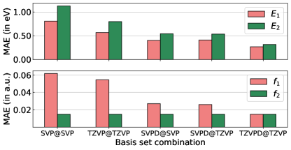
Figure 2: Errors in TD$\omega$B97XD predictions of the lowest two excitations, with various basis sets, compared to STEOM-CCSD/aug-cc-pVTZ. Results are presented for the smallest 33 molecules in bigQM7$\rm{\omega}$ with up to three CONF atoms. Mean absolute errors (MAEs) are reported for excitation energies ($E_{1}$, $E_{2}$) in the top panel, and oscillator strengths ($f_{1}$, $f_{2}$) in the bottom panel. The basis sets combination are denoted as: (TDDFT single point)@(DFT structure relaxation).

For the low-lying excited states of small molecules, equations-of-motion coupled cluster with singles doubles (EOM-CCSD)Korona and Werner (2003) and approximate second-order coupled-cluster (CC2) deliver a mean error of 0.10–0.15 eV compared to higher-level wave function methodsAdamo and Barone (1999); Laurent and Jacquemin (2013); Jacquemin et al. (2008, 2009); Loos et al. (2018, 2020a); Chrayteh et al. (2020); Loos et al. (2020b). While these methods can be made more economical by using the resolution-of-identity (RI) technique, as in RICC2Send et al. (2011) or domain-based local pseudo-natural orbital (DLPNO) variant of EOM-CCSDBerraud-Pache et al. (2020), they have known limitations when modeling the full electronic spectra of thousands of molecules. Formally, the total number of electronic states accounted for by these wave function methods scales as $\mathcal{O}(N_{o}^{2}N_{v}^{2})$, where $N_{o}$ and $N_{v}$ are the numbers of occupied and virtual MOs. Even for a small molecule such as benzene with a triple-zeta basis set, the size of the resulting electronic Hamiltonian is of the order of millions. It is well known that the iterative eigensolvers used for such large scale problems converge poorly for higher eigenvalues restricting their usage only to the lowest few electronic statesMurray et al. (1992). Hence, as of now, large scale computations of full electronic spectra across a chemical space dataset are amenable only at the time-dependent (TD) DFT-levelCasida et al. (1998); Casida and Huix-Rotllant (2012) that show an $\mathcal{O}(N_{o}N_{v})$ scaling.

While DFT offers a suitable high-throughput data generation rate, its accuracy for geometries and properties is dependent on the exchange-correlation (XC) functional. The chemical space dataset, QM9, was designed using the hybrid generalized gradient approximation (hGGA), B3LYP, with 6-31G(2$df$,$p$) basis set because of their use in the G$n$ family of composite wavefunction methodsCurtiss et al. (2011). For thermochemistry energies, B3LYP has an error of 4–5 kcal/molCurtiss et al. (2005). A recent benchmark studyDas et al. (2021) has shown the range-separated hGGAs from the $\omega$B97 familyChai and Head-Gordon (2008) to have errors in the 2–3 kcal/mol window; their performance is second only to the G$n$ methods. While curating the QM9 dataset, the dispersion corrected variant of $\omega$B97, namely $\omega$B97XD, predicted high-veracity geometries less prone to rearrangements in automated high-throughput workflowsSenthil et al. (2021). Hence, we resort to $\omega$B97XD for geometry optimization and its time-dependent variant for modeling the complete electronic excitation spectra.

The electronic excitations of the molecules in our dataset are predominantly in the deep-ultraviolet (deep-UV) to X-ray region. Since the popular flavors of TDDFT depend on the adiabatic approximation where the orbitals are relaxed to first-order as a linear response, they often fail to describe the electronic wavefunction of high-lying excited states that can substantially differ from that of the ground stateHait and Head-Gordon (2021). Such effects may be anticipated especially for excitations of long-range charge-transfer character, Rydberg-typeTozer and Handy (2000) or excitations of core electronsDreuw et al. (2003). Additionally, electronic states of doubly excited character are not accessible to the linear-response formalism of TDDFTYanai et al. (2004). However, as yet, remedies for improving TDDFT for pathological situations have not been tested over chemical space datasets. Furthermore, some of the new methods such as the orbital optimized DFT also suffer from algorithmic errors resulting in variational collapse to a low-lying stateHait and Head-Gordon (2021).

To probe the effect of basis sets on the TDDFT-level excited state properties, we selected the smallest 33 molecules with up to 3 heavy atoms as a benchmark set. Accurate modeling of oscillator strengths and high-lying electronic states require basis sets augmented with diffuse functions in order to achieve semi-quantitative accuracy. Hence, in Fig. 2, we explore $\omega$B97XD’s performance for excitation properties computed at def2SVP (SVP), def2TZVP (TZVP), def2SVPD (SVPD), and def2TZVPD (TZVPD). We use the lowest two excitation energies ($E_{1}$ and $E_{2}$) and the corresponding oscillator strengths ($f_{1}$ and $f_{2}$) with the accurate STEOM-CCSD/aug-cc-pVTZ method as the reference. Unsurprisingly, def2SVP has the largest errors across all excitation properties followed by def2TZVP, def2SVPD, and def2TZVPD. Including diffuse functions results in errors that are almost half of those from basis sets devoid of diffuse functions. The errors for all four properties obtained with the def2SVPD basis set are very similar irrespective of whether the corresponding geometries were determined with def2SVP or def2TZVP basis sets. Even though def2TZVPD offers the best accuracies, we find the computational cost for determining the full spectra of all molecules in bigQM7$\rm{\omega}$ to be very high.

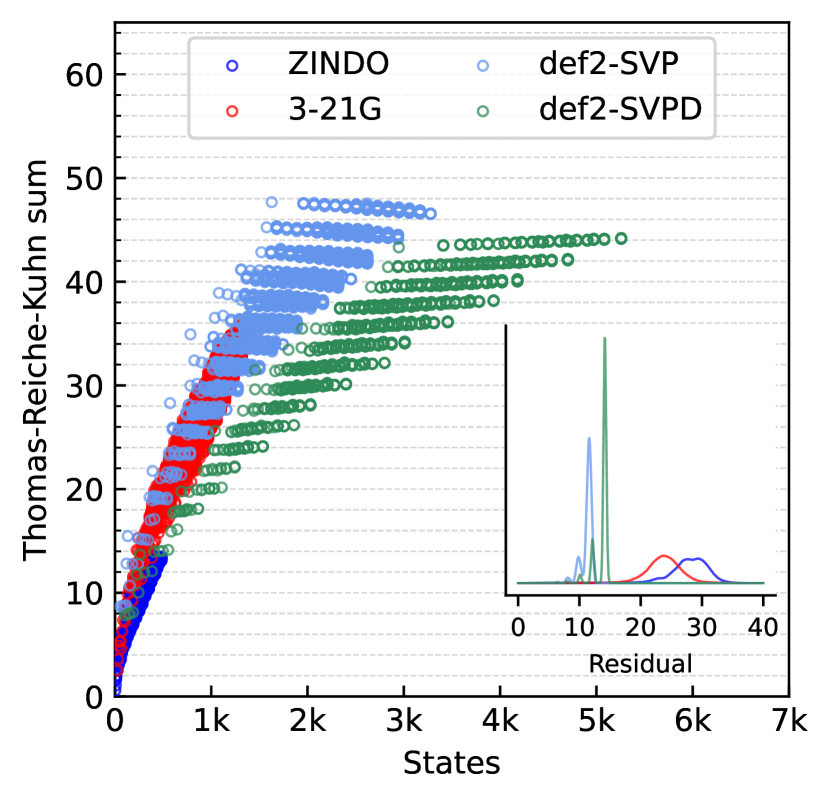
Figure 3: Basis set effect on oscillator strength sums for bigQM7$\rm{\omega}$ molecules at TD$\omega$B97XD. Sum of oscillator strengths of all states is plotted against number of allowed excitations from the ground electronic state with 3-21G, def2SVP and def2SVPD basis sets. ZINDO values are also shown for comparison. Horizontal lines mark the Thomas-Reiche-Kuhn limit an exact excited state method must coincide with. The inset shows the distribution of deviation of oscillator strength sums from total number of electrons.

Hence, we resort to the def2SVPD basis set that is cost-effective for the excited state calculations. The final target-level data used for training ML models were obtained at the TD$\omega$B97XD/def2SVPD level using geometries calculated at the $\omega$B97XD/def2SVP level. While TD$\omega$B97XD/def2SVPD level excitation spectra is by no means quantitatively accurate, for high-throughput explorations of medium-sized molecules, it still preserves broad trends that can be learned through structure-property relationships.

We also compare the performance of different methods for predicting the Thomas–Reiche–Kuhn (TRK) sum, $\sum_{k}f_{k}$. For an exact excited state method, this sum according to the TRK theorem must converge to the number of electronsTurro et al. (2017). In quantum chemistry, unfortunately, this condition is satisfied only at the full-CI limit, when all excitations (singles, doubles, triples, and so on) are accounted for at the basis set limit. ZINDO and the TD$\omega$B97XD methods are not expected to satisfy the TRK limit. We illustrate this aspect in Fig. 3 where the TRK-sum is plotted as a function of total number of states accessible. ZINDO deviates the most from the TD$\omega$B97XD/def2SVPD target because the number of excited states available is limited by two factors. Firstly, core electrons are not included in ZINDO. Secondly, semi-empirical models are implicitly based on a minimal basis set.

TDDFT modeling with 3-21G improves $\sum_{k}f_{k}$ and the total number of states compared to ZINDO. With the def2SVP and def2SVPD basis sets, $\sum_{k}f_{k}$ quantizes at even numbers with a separation of about 2. For the large basis set, def2SVPD, the number of accessible states increases, while the TRK-sum drops below the def2SVP values. We investigated the reason for this trend using methane and found the def2- basis sets to show somewhat oscillatory convergence with the basis set size. For methane, the def2SVP/def2SVPD values are 8.78/8.12, the larger basis set value agreeing better with the aug-cc-pV5Z basis set limit value of 7.82. Residual errors in ZINDO/TDDFT TRK-sums from total number of electrons are shown in the inset to Fig. 3.

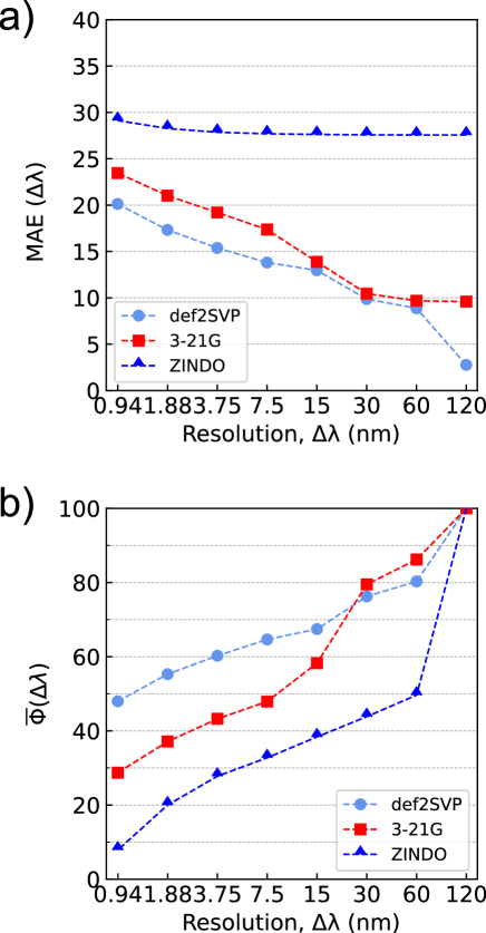
Figure 4: Accuracy metrics for binned oscillator strengths in the $\lambda\leq 120$ nm range for all molecules in bigQM7$\rm{\omega}$ : a) Mean absolute error, MAE$(\Delta\lambda)$, in atomic units (a.u.) as defined in Eq. 4, b) Mean accuracy metric for normalized spectra, $\overline{{\rm\Phi}}(\Delta\lambda)$, as defined in Eq. 6. Results are shown for ZINDO, $\omega$B97XD/3-21G and $\omega$B97XD/def2SVP for approximating $\omega$B97XD/def2SVPD level values.

IV.2 Resolution-vs.-Accuracy Trade-off

Typically, uncertainties of hybrid-DFT approximations compared to higher-level wavefunction methods are used as threshold accuracies for gauging the performance of ML models. For the bigQM7$\rm{\omega}$ dataset, along with the conventional MAE metric, we also explore a dimensionless accuracy metric for normalized spectra, $\Phi$ (see Eq. 5) and its average. Even though the electronic spectra of molecules in bigQM7$\rm{\omega}$ span a wavelength range until 850 nm, $>99\%$ of the spectra lie in the deep UV to X-ray range ($10-120$ nm). Such a trend has been noted before for small organic moleculesZheng et al. (2016). Hence in this study, we fix the spectral range ($\lambda_{\rm spectrum}$) to 0–120 nm and bin oscillator strengths at various wavelength resolutions ($\Delta\lambda$) according to Eq. 3. For a given $\Delta\lambda$, we compare MAE and $\overline{\Phi}$ of predictions from ZINDO, $\omega$B97XD/3-21G, or $\omega$B97XD/def2SVP levels with that of the $\omega$B97XD/def2SVPD values (see Fig. 4). For atomization energies and low-lying excitation energies, these values are 3–4 kcal/mol, and 0.2–0.3 eVLoos et al. (2020b), respectively. For oscillator strengths, such a threshold has not been established, especially for chemical space datasets.

In Fig. 4a, the MAE of ZINDO shows a smaller variation with $\Delta\lambda$. For the extreme case of $\Delta\lambda=120$ nm, where the oscillator strengths of all states are summed in a bin, ZINDO’s MAE saturates to about 27.5 a.u implying a systematic error in ZINDO. For the desired resolution of 0.94 nm, ZINDO’s error increases only slightly. The MAEs improve for the spectra calculated with $\omega$B97XD/3-21G. For the single bin case, the 3-21G results also indicate a systematic error albeit of a smaller magnitude compared to ZINDO. The errors are further quenched for the def2SVP basis set, which for a resolution of $\Delta\lambda=0.94$ nm has an MAE of about 20 a.u. Overall, the MAE-vs-$\Delta\lambda$ dependency becomes stronger in the order: ZINDO ¡ $\omega$B97XD/3-21G ¡ $\omega$B97XD/def2SVP. This trend is in agreement with the magnitude of TRK-sum as predicted by these methods, see Fig. 3. In general, a similar trend is noted also for individual oscillator strengths.

As pointed out in Section-III, for the limiting case of $\Delta\lambda=120$ nm, when all oscillator strengths are summed in one bin, the $\Phi$ is 100 for ZINDO, $\omega$B97XD/3-21G, and $\omega$B97XD/def2SVP methods compared to the target $\omega$B97XD/def2SVPD (see Fig. 4b). With increasing resolution, the methods diverge from the target, ZINDO showing the largest deviation from $\omega$B97XD/def2SVPD. For a desirable resolution of 1% of $\lambda_{\rm spectrum}$, $\Delta\lambda\thickapprox 1$ nm, 3-21G and def2SVP predictions result in $\Phi$s of $30-50$ compared to the target, while ZINDO has a worse score $\thickapprox 10$. The reason for poor $\Phi$s of ZINDO predictions at small resolution is because core states are absent in ZINDO, limiting the spectral range to $>19.8$ nm. In contrast, the density of the states at the target TD$\omega$B97XD level is high in the short wavelength domain. Applying bin-specific systematic corrections can improve both the accuracy metrics for all three methods: ZINDO, $\omega$B97XD/3-21G, and $\omega$B97XD/def2SVP. However, such corrections may not result in uniform improvement throughout the spectral range. For instance, at short wavelength regions where the TD$\omega$B97XD spectra are sharp, ZINDO lacks these lines. However, systematic corrections may result in vanishing MAE for the wrong reason. On the other hand, the effect of such corrections will be less severe for the normalized metric, $\overline{\Phi}$. Hence, we do not apply bin-specific systematic corrections in this analyses. Overall, at the desired resolution of 0.94 nm, among the methods inspected here, the one with larger MAE has the smaller accuracy metric, $\overline{\Phi}$ and vice versa.

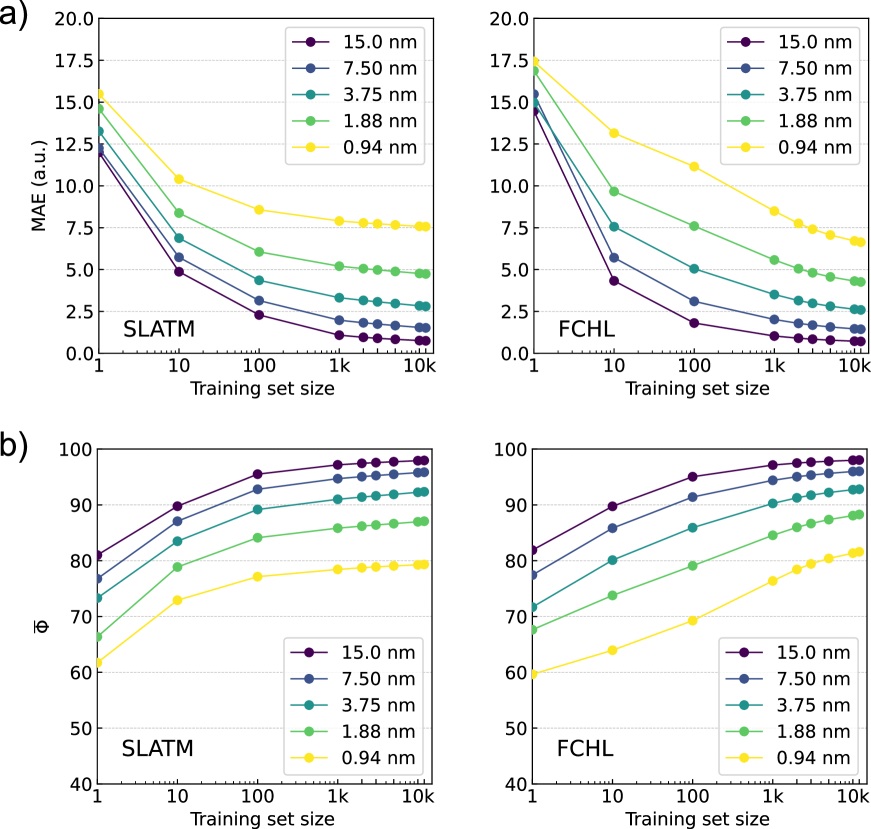
Figure 5: Learning rates based on accuracy metrics for out-of-sample predictions of $\omega$B97XD/def2SVPD level binned oscillator strengths (in the $\leq 120$ nm region) for the bigQM7$\rm{\omega}$ dataset: Panel a reports MAE in a.u. and Panel b reports $\overline{{\rm\Phi}}$ as functions of training set size for ML models trained using the single-kernel approach with SLATM (left) and FCHL (right) representations generated using UFF-level geometries.

IV.3 Reconstruction of electronic spectra with ML models

In Fig. 5, we report learning rates based on MAE and $\Phi$ for predicting binned oscillator strengths (defined in Eq.3) using KRR-FCHL and KRR-SLATM models for various training set sizes and spectral resolutions. For poor resolutions, we find small MAEs and large $\Phi$s already at the offset of learning curves. For large training set sizes and at all resolutions FCHL slightly outperforms SLATM. While the SLATM model saturates to an MAE of $\thickapprox$7.5 a.u. and $\overline{\Phi}\thickapprox 80$ for 0.94 nm resolution FCHL model shows improved learning rates, suggesting its scope for modeling full-electronic spectra of larger datasets. These findings indicate that it is possible to employ ML modeling for reconstructing electronic spectra at a high-resolution. Since the ML models were trained on $p_{i}$ (binned oscillator strengths), the predicted spectra can be compared with the reference TD$\omega$B97XD spectra similarly binned. The prediction error of the reconstructed spectrum may be quantified either as a sum of absolute differences, or using the accuracy metric upon normalizing the binned intensities. The definitions of the error metric do not influence the ML-reconstruction of the spectra, but they serve merely to quantify the mean prediction accuracy.

The spectra reconstructed with these models do not contain any state-specific information, but rather indicate the intensity of dipole absorption in a finite wavelength window. At the limit of very small $\Delta\lambda$, these bins will correspond to individual transitions. It is worth noting that for a resolution of 0.94 nm, TD$\omega$B97XD/def2SVP spectra agree with that of the target-level only with a score of $\thickapprox 47$. The $\Phi$ drops even further for TD$\omega$B97XD/3-21G ($\thickapprox 29$) and ZINDO ($\thickapprox 9$) levels. The learning rates in our evaluatory $\Delta$-MLRamakrishnan et al. (2015a) calculations using ZINDO, TD$\omega$B97XD/3-21G, or even TD$\omega$B97XD/def2SVP baseline spectra were inferior than modeling directly on the TD$\omega$B97XD/def2SVPD target. Hence, all ML models were trained directly on the target.

In Fig. 6, we present the entire spectrum of an out-of-sample molecule, cyclohexanone, reconstructed using FCHL-ML models with 1k training examples at three different wavelength resolutions–3.75 nm, 1.88 nm, and 0.94 nm. Since the ML models were trained using geometries at the UFF level, these out-of-sample predictions were performed with in a matter of seconds. As a part of the supplementary material, we provide a sample code for generating the spectrum using a trained FCHL models (see Data Availability). For $\Delta\lambda=3.75$ nm, the ML-reconstructed spectrum agrees with the target TD$\omega$B97XD spectrum with a $\Phi$ of 86.5. This accuracy drops for higher resolutions due to the fine details present in the target spectrum. Also, with increase in resolution we note a reduction in the spectral heights in order to conserve the total area under the spectrum. For the desired value of $\Delta\lambda=0.94$ nm, the spectrum of cyclohexanone is reconstructed with a score of 72.6 which is slightly lower than the mean score reported for out-of-sample predictions in Fig. 5.

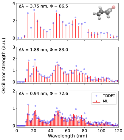
Figure 6: Electronic excitation spectrum of of cyclohexanone, reconstructed at 3.75 nm, 1.88 nm, and 0.94 nm resolutions using a 1k FCHL-KRR-ML model trained on binned oscillator strengths ($p_{i}$ in Eq.3) at the TD$\omega$B97XD/def2SVPD target-level. Accuracy metric for normalized spectra, $\Phi$, compared to TD$\omega$B97XD reference values calculated according to Eq. 5 are also given.

Further, for the highest resolution explored here, we present the ML reconstructed spectra for three more randomly drawn out-of-sample molecules in Fig. 7. For all these molecules, the prediction is better than for cyclohexanone and are illustrative of the model’s mean out-of-sample performance. While the reference TD$\omega$B97XD-level binned oscillator strengths are always $>0$, the predicted values are not bound, hence, we notice small negative intensities for 5,5‐dimethyl‐4,5‐dihydro‐1H‐pyrazole. For all four out-of-sample molecules considered here, the spectral intensities are low for $\lambda>100$ nm because of the corresponding excitations in this region is sparse. We believe that ML strategy for spectral reconstruction reported in this study will hold even at the interesting long-wavelength domain when these models are trained on adequate examples.

V Data-mining in MolDis

The dataset collected in lieu of this study, justifies an endeavor to make it accessible to the wider community. While unstructured datasets require an additional step of data extraction, a data-mining platform allows us to rapidly perform multi-property querying and screening. Our data-mining platform MolDisKrishnan et al. is well-suited to cater to such requirements and hence, we are hosting property-oriented mining platforms for minimum energy ground-state structures of 12880 molecules obtained at the $\omega$B97XD/def2SVP & $\omega$B97XD/def2TZVP levels at https://moldis.tifrh.res.in/datasets.html with both ground-state and excited-state properties.

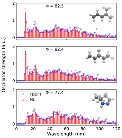
Figure 7: Electronic excitation spectrum of three randomly selected molecules—(3Z)‐5‐fluoro‐4‐methylpenta‐1,3‐diene, 1‐fluoropentan‐3‐ol, and 5,5‐dimethyl‐4,5‐dihydro‐1H‐pyrazole — reconstructed at 0.94 nm resolution using a 1k FCHL-KRR-ML. The model was trained on TD$\omega$B97XD/def2SVPD electronic spectra in the $\lambda\leq 120$ nm wavelength range. Accuracy metric for normalized spectra, $\Phi$, compared to TD$\omega$B97XD reference values calculated according to Eq. 5 are also given.

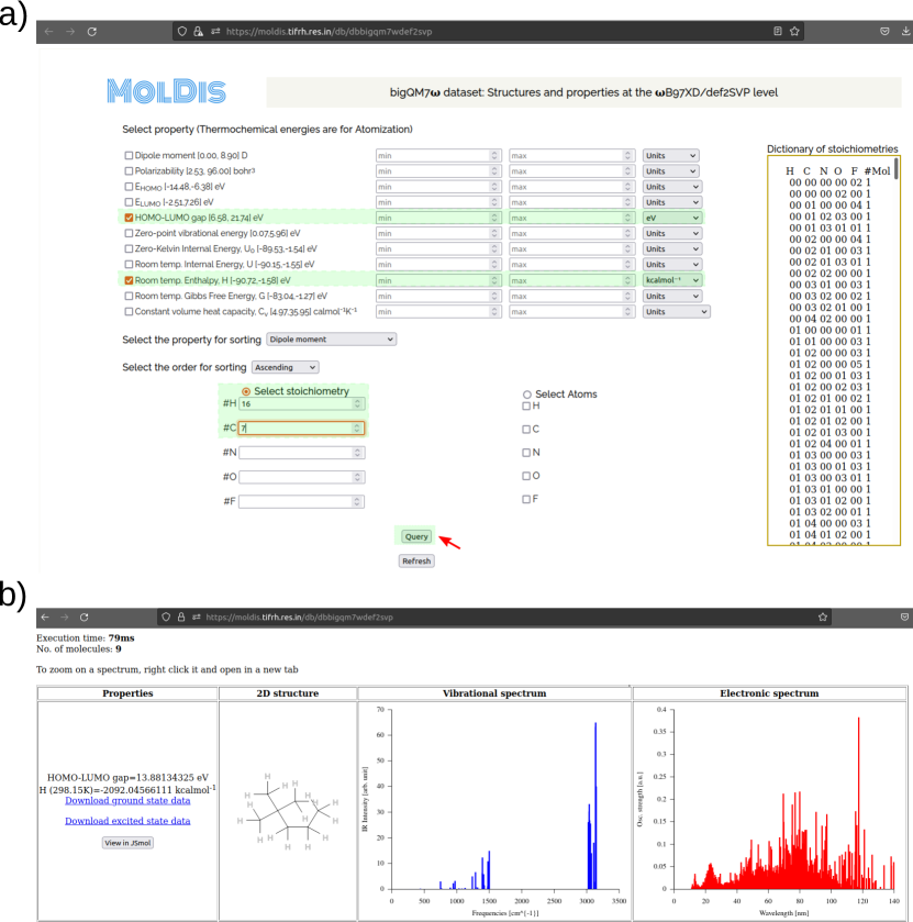
Figure 8: Screenshots of the web-based data-mining platform for querying the bigQM7$\omega$ dataset: (a) query page and (b) results page. The example shows how to query the HOMO-LUMO gap and room temperature atomization enthalpy of hydrocarbons with the C₇H₁₆ stoichiometry. Separate links are provided at https://moldis.tifrh.res.in/datasets.html for accessing minimum energy geometries, ground state properties, and vibrational spectra at the $\omega$B97XD/def2SVP and $\omega$B97XD/def2TZVP levels. Electronic spectra calculated at the TD$\omega$B97XD/def2SVPD are also provided.

In Fig. 8, we present a representative property query in the MolDis platform and the corresponding results. On accessing the def2SVP tab in the bigQM7$\omega$ Datasets page, we arrive at the corresponding query page. As noted in Fig. 8a, there are 11 ground state properties—dipole moment, polarizability, $E_{\rm HOMO}$, $E_{\rm LUMO}$, $E_{\rm LUMO-HOMO}$, zero-point vibrational energy, zero-Kelvin internal energy ($U_{0}$), room temperature internal energy ($U$), room temperature enthalpy ($H$), room temperature Gibbs free energy ($G$), and constant volume heat capacity ($C_{v}$)—with available property ranges reported next to them. For a query, users need to enter values with in the property range with appropriate units selected and click on the Query button. The search can be further customized upon including multiple properties in the query and display them in ascending or descending order with respect to any property from the corresponding drop-down window. We have also enabled an option to query based on composition. In the bottom half of Fig. 8a, users can select either a set of atoms or any valid stoichiometry as listed on the right side of the query page. Upon making a successful query, users are presented with results (Fig. 8b), where the Cartesian coordinates, vibrational and electronic spectra are provided along with the magnitudes of queried properties in desired units. A JSMol applet enables visitors to visualize the structures on their browser upon clicking the “View in JSMol” button. Further, upon a fruitful query, both ground-state and excited-state properties for every molecule is presented to the visitor as downloadable files on the results page (Fig. 8b). This platform allows access to ab initio properties collected via high-throughput chemical space investigations to the community in a user-friendly fashion, hence, widening the applicability scope of the bigQM7$\rm{\omega}$ dataset.

VI Conclusions

In this work we present the new chemical space dataset, bigQM7$\rm{\omega}$ , containing 12880 molecules with up to 7 atoms of CONF. Geometry optimizations of the bigQM7$\rm{\omega}$ molecules have been performed with the ConnGO workflow ensuring veracity in the covalent bonding connectivities encoded in their SMILES representation. Minimum energy geometries and harmonic vibrational wavenumbers are reported at the accurate, range-separated hybrid DFT level $\omega$B97XD using def2SVP and def2TZVP basis sets. This level was selected because it has been previously shown to result in efficient geometry predictions for chemical space datasetsSenthil et al. (2021). We report electronic excited state results at the TD$\omega$B97XD level using the def2SVPD basis set containing diffuse functions that are necessary for improved modeling of oscillator strengths, and high-lying states in general. Even for the low-lying excited states of the bigQM7$\rm{\omega}$ molecules, we found TD$\omega$B97XD/def2SVPD to deliver more accurate results than the $\omega$B97XD/def2TZVP combination when benchmarked against STEOM-CCSD/aug-cc-pVTZ reference values. For all molecules, full electronic spectra are calculated covering all possible excitations allowed by the TD$\omega$B97XD framework. For the small molecules H₂O, NH₃, and CH₄ the resulting number of excited states modeled amounts to 188, 156 and 136, respectively, while for large molecules such as toluene or $n$-heptane the total number of excited states reported is 3222 and 5258, respectively. Our preliminary findings have shown that generating the TD$\omega$B97XD results with the even larger basis set def2TZVPD to require several-fold increase in CPU time. However, when aiming at only a few low-lying states, our results can be improved when using approximate correlated methods such as DLPNO-STEOM-CCSD(T) or RI-CC2.

For ML modeling of the full electronic spectra, we propose an approach using locally integrated spectral intensities at various wavelength resolutions. We illustrate the existence of a resolution-vs.-accuracy dilemma for comparing full electronic spectra from different methods. The mapping between the electronic spectra and the global molecular structure-based representations improves only when the intensities are binned at a finite resolution. Semi-quantitative agreement between methods is reached only at the expense of resolution. Compared to this, ML models deliver better accuracies at a sub-nm resolution when training on fraction of the dataset. For accurate reconstruction of full electronic spectra across chemical space with a resolution of $<1$ nm, we recommend FCHL-KRR-ML. Further, it may be possible to improve the ML model’s performance in the long wavelength region using varying resolutions at different spectral regions. However, testing this idea requires new datasets comprising adequate data at the desired wavelength domain.

Our goal is to provide a proof-of-concept for ML modeling of binned electronic spectra and demonstrate accurate spectral reconstruction. Unfortunately, the size of the dataset limits the rigor of quantum mechanical methods and basis sets used to estimate the target spectra for ML models. While we used range-separated hybrid DFT with moderately large basis sets containing diffuse functions, inherent deficiencies in the method challenge the accuracy of the target. Further, the small size of the molecules in bigQM7$\rm{\omega}$ implied excitations modeled are in the far UV region. However, ML modeling reproduced target spectra at accuracies lower than that arising from deficiencies in the quantum mechanical methods. This suggests that replacing the target with properties estimated from high-fidelity methods will be adequately captured through ML modeling.

Improvements of ML modeling of excited state requires development of new local descriptors that can map to the chromophores responsible for excitation. For this, an automated protocol to characterize electronic excited-states should be developed for high-throughput chemical space design frameworks. This allows the opportunity to explore chemically diverse photochemically interesting molecules, such as dyes, active in the UV/visible domain and investigate chromophore’s/auxochrome’s influence on spectra. Another possibility is to cluster the electronic spectral data according to chromophores Ramakrishnan et al. (2015b); Mazouin et al. (2021) or by unsupervised learningCheng et al. (2022). However, one must ensure that for generating accurate models, each cluster must be adequately represented in the training set. In order to facilitate further studies, we provide all data generated for this study in public domains.

VII Data Availability

Structures, ground state properties and electronic spectra of the bigQM7$\rm{\omega}$ dataset are available at https://moldis-group.github.io/bigQM7w, see  Ref.62. Input and output files of corresponding calculations are deposited in the NOMAD repository (https://dx.doi.org/10.17172/NOMAD/2021.09.30-1), see  Ref.63. A data-mining platform is available at https://moldis.tifrh.res.in/index.html.

VIII Acknowledgments

We acknowledge support of the Department of Atomic Energy, Government of India, under Project Identification No. RTI 4007. All calculations have been performed using the Helios computer cluster, which is an integral part of the MolDis Big Data facility, TIFR Hyderabad (http://moldis.tifrh.res.in).

IX Author Contributions

PK and RR conceptualised the project and methodology. SC and RR were involved in writing, reviewing, and editing the manuscript. SC and RR maintain the project content in GitHub and MolDis. All authors were involved in data generation/curation, analysis and visualization. Software development, resource/funding acquisition were done by RR. RR supervised PK and SC.

Conflicts of interest

“There are no conflicts to declare”.

References

- Steiner et al. (2019) S. Steiner, J. Wolf, S. Glatzel, A. Andreou, J. M. Granda, G. Keenan, T. Hinkley, G. Aragon-Camarasa, P. J. Kitson, D. Angelone, et al., Science 363, 1 (2019).
- Christensen et al. (2021) M. Christensen, L. P. Yunker, F. Adedeji, F. Häse, L. M. Roch, T. Gensch, G. dos Passos Gomes, T. Zepel, M. S. Sigman, A. Aspuru-Guzik, et al., Commun. Chem. 4, 1 (2021).
- Stach et al. (2021) E. Stach, B. DeCost, A. G. Kusne, J. Hattrick-Simpers, K. A. Brown, K. G. Reyes, J. Schrier, S. Billinge, T. Buonassisi, I. Foster, et al., Matter 4, 2702 (2021).
- Gromski et al. (2020) P. S. Gromski, J. M. Granda, and L. Cronin, Trends in Chemistry 2, 4 (2020).
- Li et al. (2021) X. Li, P. M. Maffettone, Y. Che, T. Liu, L. Chen, and A. I. Cooper, Chem. Sci. 12, 10742 (2021).
- Bai et al. (2019) Y. Bai, L. Wilbraham, B. J. Slater, M. A. Zwijnenburg, R. S. Sprick, and A. I. Cooper, J. Am. Chem. Soc. 141, 9063 (2019).
- Mathew et al. (2014) S. Mathew, A. Yella, P. Gao, R. Humphry-Baker, B. F. Curchod, N. Ashari-Astani, I. Tavernelli, U. Rothlisberger, M. K. Nazeeruddin, and M. Grätzel, Nat. Chem. 6, 242 (2014).
- Abreha et al. (2019) B. G. Abreha, S. Agarwal, I. Foster, B. Blaiszik, and S. A. Lopez, J. Phys. Chem. Lett. 10, 6835 (2019).
- Sampedro (2011) D. Sampedro, Phys. Chem. Chem. Phys. 13, 5584 (2011).
- Losantos et al. (2017) R. Losantos, I. Funes-Ardoiz, J. Aguilera, E. Herrera-Ceballos, C. García-Iriepa, P. J. Campos, and D. Sampedro, Angew. Chem. 129, 2676 (2017).
- Hachmann et al. (2011) J. Hachmann, R. Olivares-Amaya, S. Atahan-Evrenk, C. Amador-Bedolla, R. S. Sánchez-Carrera, A. Gold-Parker, L. Vogt, A. M. Brockway, and A. Aspuru-Guzik, J. Phys. Chem. Lett. 2, 2241 (2011).
- Pyzer-Knapp et al. (2015) E. O. Pyzer-Knapp, K. Li, and A. Aspuru-Guzik, J. Phys. Chem. Lett. 25, 6495 (2015).
- Rupp et al. (2012) M. Rupp, A. Tkatchenko, K.-R. Müller, and O. A. von Lilienfeld, Phys. Rev. Lett. 108, 058301 (2012).
- Ramakrishnan and von Lilienfeld (2017) R. Ramakrishnan and O. A. von Lilienfeld, Rev. Comput. Chem. 30, 225 (2017).
- von Lilienfeld (2018) O. A. von Lilienfeld, Angew. Chem. Int. Ed. 57, 4164 (2018).
- Ramakrishnan and von Lilienfeld (2015) R. Ramakrishnan and O. A. von Lilienfeld, CHIMIA 69, 182 (2015).
- Ramakrishnan et al. (2015a) R. Ramakrishnan, P. O. Dral, M. Rupp, and O. A. von Lilienfeld, J. Chem. Theory Comput. 11, 2087 (2015a).
- Rupp et al. (2015) M. Rupp, R. Ramakrishnan, and O. A. von Lilienfeld, J. Phys. Chem. Lett. 6, 3309 (2015).
- Gerrard et al. (2020) W. Gerrard, L. A. Bratholm, M. J. Packer, A. J. Mulholland, D. R. Glowacki, and C. P. Butts, Chem. Sci. 11, 508 (2020).
- Gupta et al. (2021) A. Gupta, S. Chakraborty, and R. Ramakrishnan, Mach. Learn.: Sci. Technol 2, 035010 (2021).
- Hansen et al. (2015) K. Hansen, F. Biegler, R. Ramakrishnan, W. Pronobis, O. A. von Lilienfeld, K.-R. Müller, and A. Tkatchenko, J. Phys. Chem. Lett. 6, 2326 (2015).
- Faber et al. (2018) F. A. Faber, A. S. Christensen, B. Huang, and O. A. von Lilienfeld, J. Chem. Phys. 148, 241717 (2018).
- Qiao et al. (2020) Z. Qiao, M. Welborn, A. Anandkumar, F. R. Manby, and T. F. Miller III, J. Chem. Phys. 153, 124111 (2020).
- Unke and Meuwly (2019) O. T. Unke and M. Meuwly, J. Chem. Theory Comput. 15, 3678 (2019).
- Schütt et al. (2017) K. Schütt, P.-J. Kindermans, H. E. Sauceda Felix, S. Chmiela, A. Tkatchenko, and K.-R. Müller, Advances in neural information processing systems 30, 1 (2017).
- Faber et al. (2017) F. A. Faber, L. Hutchison, B. Huang, J. Gilmer, S. S. Schoenholz, G. E. Dahl, O. Vinyals, S. Kearnes, P. F. Riley, and O. A. von Lilienfeld, J. Chem. Theory Comput. 13, 5255 (2017).
- Prezhdo (2021) O. V. Prezhdo, Acc. Chem. Res. 54, 4239 (2021), pMID: 34756013, https://doi.org/10.1021/acs.accounts.1c00525 .
- Lam et al. (2020) J. Lam, S. Abdul-Al, and A.-R. Allouche, J. Chem. Theory Comput. 16, 1681 (2020).
- Kananenka et al. (2019) A. A. Kananenka, K. Yao, S. A. Corcelli, and J. Skinner, J. Chem. Theory Comput. 15, 6850 (2019).
- Çaylak et al. (2019) O. Çaylak, A. Yaman, and B. Baumeier, J. Chem. Theory Comput. 15, 1777 (2019).
- Vela et al. (2021) S. Vela, A. Fabrizio, K. R. Briling, and C. Corminboeuf, J. Phys. Chem. Lett. 12, 5957 (2021).
- Grisafi et al. (2018) A. Grisafi, A. Fabrizio, B. Meyer, D. M. Wilkins, C. Corminboeuf, and M. Ceriotti, ACS Cent. Sci. 5, 57 (2018).
- Ramakrishnan et al. (2015b) R. Ramakrishnan, M. Hartmann, E. Tapavicza, and O. A. von Lilienfeld, J. Chem. Phys. 143, 084111 (2015b).
- Tapavicza et al. (2021) E. Tapavicza, G. F. von Rudorff, D. O. De Haan, M. Contin, C. George, M. Riva, and O. A. von Lilienfeld, Environ. Sci. Technol. 55, 8447– (2021).
- Çaylak and Baumeier (2021) O. Çaylak and B. Baumeier, J. Chem. Theory Comput. 17, 4891 (2021).
- Westermayr and Marquetand (2020a) J. Westermayr and P. Marquetand, J. Chem. Phys. 153, 154112 (2020a).
- Westermayr and Marquetand (2020b) J. Westermayr and P. Marquetand, Chem. Rev. 121, 9873–9926 (2020b).
- Dral and Barbatti (2021) P. O. Dral and M. Barbatti, Nat. Rev. Chem. 5, 388 (2021).
- Rankine and Penfold (2021) C. D. Rankine and T. J. Penfold, J. Phys. Chem. A 125, 4276 (2021).
- Hansen et al. (2013) K. Hansen, G. Montavon, F. Biegler, S. Fazli, M. Rupp, M. Scheffler, O. A. von Lilienfeld, A. Tkatchenko, and K.-R. Muller, J. Chem. Theory Comput. 9, 3404 (2013).
- von Lilienfeld et al. (2015) O. A. von Lilienfeld, R. Ramakrishnan, M. Rupp, and A. Knoll, Int. J. Quantum Chem. 115, 1084 (2015).
- Huang et al. (2005) X. Huang, B. J. Braams, and J. M. Bowman, J. Chem. Phys. 122, 044308 (2005).
- Behler (2015) J. Behler, Int. J. Quantum Chem. 115, 1032 (2015).
- Manzhos and Carrington Jr (2020) S. Manzhos and T. Carrington Jr, Chem. Rev. 121, 10187–10217 (2020).
- Hohenberg and Kohn (1964) P. Hohenberg and W. Kohn, Phys. Rev. 136, B864 (1964).
- Runge and Gross (1984) E. Runge and E. K. Gross, Phys. Rev. Lett. 52, 997 (1984).
- Mahmoud et al. (2020) C. B. Mahmoud, A. Anelli, G. Csányi, and M. Ceriotti, Phys. Rev. B 102, 235130 (2020).
- Westermayr and Maurer (2021) J. Westermayr and R. J. Maurer, Chem. Sci. 12, 10755 –10764 (2021).
- Ramakrishnan et al. (2014) R. Ramakrishnan, P. O. Dral, M. Rupp, and O. A. von Lilienfeld, Sci. Data 1, 1 (2014).
- Liu et al. (2021) Z. Liu, L. Lin, Q. Jia, Z. Cheng, Y. Jiang, Y. Guo, and J. Ma, J. Chem. Inf. Model. 61, 1066 (2021).
- Mazouin et al. (2021) B. Mazouin, A. A. Schöpfer, and O. A. von Lilienfeld, arXiv preprint arXiv:2110.02596 , 1 (2021).
- Fink et al. (2005) T. Fink, H. Bruggesser, and J.-L. Reymond, Angew. Chem. Int. Ed. 44, 1504 (2005).
- Fink and Reymond (2007) T. Fink and J.-L. Reymond, J. Chem. Inf. Model. 47, 342 (2007).
- Blum and Reymond (2009) L. C. Blum and J.-L. Reymond, J. Am. Chem. Soc. 131, 8732 (2009).
- Ruddigkeit et al. (2012) L. Ruddigkeit, R. Van Deursen, L. C. Blum, and J.-L. Reymond, J. Chem. Inf. Model. 52, 2864 (2012).
- Montavon et al. (2013) G. Montavon, M. Rupp, V. Gobre, A. Vazquez-Mayagoitia, K. Hansen, A. Tkatchenko, K.-R. Müller, and O. A. von Lilienfeld, New J. Phys. 15, 095003 (2013).
- Hoja et al. (2021) J. Hoja, L. M. Sandonas, B. G. Ernst, A. Vazquez-Mayagoitia, R. A. DiStasio Jr, and A. Tkatchenko, Sci. Data 8, 1 (2021).
- Perdew et al. (1996) J. P. Perdew, K. Burke, and M. Ernzerhof, Phys. Rev. Lett. 77, 3865 (1996).
- Adamo and Barone (1999) C. Adamo and V. Barone, J. Chem. Phys. 110, 6158 (1999).
- Becke (1993) A. D. Becke, J. Chem. Phys. 98, 1372 (1993).
- Chai and Head-Gordon (2008) J.-D. Chai and M. Head-Gordon, Phys. Chem. Chem. Phys. 10, 6615 (2008).
- Kayastha and Ramakrishnan (2021a) P. Kayastha and R. Ramakrishnan, “bigQM7: A high-quality dataset of ground-state properties and excited state spectra of 12880 molecules containing up to 7 atoms of CONF,” (2021a).
- Kayastha and Ramakrishnan (2021b) P. Kayastha and R. Ramakrishnan, “bigQM7: Unstructured data on NOMAD repository,” (2021b).
- Rappé et al. (1992) A. K. Rappé, C. J. Casewit, K. Colwell, W. A. Goddard III, and W. M. Skiff, J. Am. Chem. Soc. 114, 10024 (1992).
- O’Boyle et al. (2011) N. M. O’Boyle, M. Banck, C. A. James, C. Morley, T. Vandermeersch, and G. R. Hutchison, J. Cheminformatics 3, 1 (2011).
- Senthil et al. (2021) S. Senthil, S. Chakraborty, and R. Ramakrishnan, Chem. Sci. 12, 5566 (2021).
- Weigend and Ahlrichs (2005) F. Weigend and R. Ahlrichs, Phys. Chem. Chem. Phys. 7, 3297 (2005).
- Ridley and Zerner (1973) J. Ridley and M. Zerner, Theor. Chim. Acta 32, 111 (1973).
- Frisch et al. (2016) M. Frisch, G. Trucks, H. Schlegel, G. Scuseria, M. Robb, J. Cheeseman, G. Scalmani, V. Barone, G. Petersson, H. Nakatsuji, et al., “Gaussian 16,” (2016).
- Nooijen and Bartlett (1997) M. Nooijen and R. J. Bartlett, J. Chem. Phys. 107, 6812 (1997).
- Neese (2012) F. Neese, Rev.: Comput. Mol. Sci 2, 73 (2012).
- Neese (2018) F. Neese, WIREs Comput. Mol. Sci. 8, e1327 (2018).
- Schölkopf et al. (2002) B. Schölkopf, A. J. Smola, F. Bach, et al., Learning with kt vector machines, regularization, optimization, and beyond (MIT press, 2002).
- Christensen et al. (2020) A. S. Christensen, L. A. Bratholm, F. A. Faber, and O. Anatole von Lilienfeld, J. Chem. Phys. 152, 044107 (2020).
- Huang and von Lilienfeld (2020) B. Huang and O. A. von Lilienfeld, Nat. Chem. 12, 945 (2020).
- Kayastha and Ramakrishnan (2021c) P. Kayastha and R. Ramakrishnan, Mach. Learn.: Sci. Technol 2, 035035 (2021c).
- Van Loan and Golub (1996) C. F. Van Loan and G. Golub, Matrix computations (Johns Hopkins studies in mathematical sciences) (The Johns Hopkins University Press, 1996).
- Christensen et al. (2017) A. Christensen, F. Faber, B. Huang, L. Bratholm, A. Tkatchenko, K. Muller, and O. von Lilienfeld, “QML: A python toolkit for quantum machine learning,” (2017).
- Turro et al. (2017) N. J. Turro, V. Ramamurthy, and J. C. Scaiano, Modern molecular photochemistry of organic molecules (Viva Books University Science Books, Sausalito, 2017).
- Loos et al. (2018) P.-F. Loos, A. Scemama, A. Blondel, Y. Garniron, M. Caffarel, and D. Jacquemin, J. Chem. Theory Comput. 14, 4360 (2018).
- Loos et al. (2020a) P.-F. Loos, F. Lipparini, M. Boggio-Pasqua, A. Scemama, and D. Jacquemin, J. Chem. Theory Comput. 16, 1711 (2020a).
- Loos et al. (2020b) P.-F. Loos, A. Scemama, M. Boggio-Pasqua, and D. Jacquemin, J. Chem. Theory Comput. 16, 3720 (2020b).
- Schreiber et al. (2008) M. Schreiber, M. R. Silva-Junior, S. P. Sauer, and W. Thiel, The Journal of chemical physics 128, 134110 (2008).
- Korona and Werner (2003) T. Korona and H.-J. Werner, J. Chem. Phys. 118, 3006 (2003).
- Laurent and Jacquemin (2013) A. D. Laurent and D. Jacquemin, Int. J. Quantum Chem. 113, 2019 (2013).
- Jacquemin et al. (2008) D. Jacquemin, E. A. Perpete, G. E. Scuseria, I. Ciofini, and C. Adamo, J. Chem. Theory Comput. 4, 123 (2008).
- Jacquemin et al. (2009) D. Jacquemin, V. Wathelet, E. A. Perpete, and C. Adamo, J. Chem. Theory Comput. 5, 2420 (2009).
- Chrayteh et al. (2020) A. Chrayteh, A. Blondel, P.-F. Loos, and D. Jacquemin, J. Chem. Theory Comput. 17, 416 (2020).
- Send et al. (2011) R. Send, M. Kühn, and F. Furche, J. Chem. Theory Comput. 7, 2376 (2011).
- Berraud-Pache et al. (2020) R. Berraud-Pache, F. Neese, G. Bistoni, and R. Izsák, J. Chem. Theory Comput. 16, 564 (2020).
- Murray et al. (1992) C. W. Murray, S. C. Racine, and E. R. Davidson, J. Comput. Phys. 103, 382 (1992).
- Casida et al. (1998) M. E. Casida, C. Jamorski, K. C. Casida, and D. R. Salahub, J. Chem. Phys. 108, 4439 (1998).
- Casida and Huix-Rotllant (2012) M. E. Casida and M. Huix-Rotllant, Annu. Rev. Phys. Chem. 63, 287 (2012).
- Curtiss et al. (2011) L. A. Curtiss, P. C. Redfern, and K. Raghavachari, Wiley Interdiscip. Rev. Comput. Mol. Sci. 1, 810 (2011).
- Curtiss et al. (2005) L. A. Curtiss, P. C. Redfern, and K. Raghavachari, J. Chem. Phys. 123, 124107 (2005).
- Das et al. (2021) S. K. Das, S. Chakraborty, and R. Ramakrishnan, J. Chem. Phys. 154, 044113 (2021).
- Hait and Head-Gordon (2021) D. Hait and M. Head-Gordon, J. Phys. Chem. Lett. 12, 4517 (2021).
- Tozer and Handy (2000) D. J. Tozer and N. C. Handy, Phys. Chem. Chem. Phys. 2, 2117 (2000).
- Dreuw et al. (2003) A. Dreuw, J. L. Weisman, and M. Head-Gordon, J. Chem. Phys. 119, 2943 (2003).
- Yanai et al. (2004) T. Yanai, D. P. Tew, and N. C. Handy, Chem. Phys. Lett. 393, 51 (2004).
- Zheng et al. (2016) L. Zheng, N. F. Polizzi, A. R. Dave, A. Migliore, and D. N. Beratan, J. Phys. Chem. A 120, 1933 (2016).
- (102) S. Krishnan, A. Ghosh, M. Gupta, P. Kayastha, S. Senthil, S. K. Das, K. S. Chandra, C. Sabyasachi, A. Gupta, and R. Ramakrishnan, “MolDis: A Big Data Analytics Platform for Molecular Discovery,” https://moldis.tifrh.res.in/.
- Cheng et al. (2022) L. Cheng, J. Sun, and T. F. Miller III, arXiv preprint arXiv:2204.09831 , 1 (2022).