An analysis on metric-driven multi-target sensor management: GOSPA versus OSPA

Abstract

This paper presents an analysis on sensor management using a cost function based on a multi-target metric, in particular, the optimal subpattern-assignment (OSPA) metric, the unnormalised OSPA (UOSPA) metric and the generalised OSPA (GOSPA) metric ($\alpha=2$). We consider the problem of managing an array of sensors, where each sensor is able to observe a region of the surveillance area, not covered by other sensors, with a given sensing cost. We look at the case in which there are far-away, independent potential targets, at maximum one per sensor region. In this set-up, the optimal action using GOSPA is taken for each sensor independently, as we may expect. On the contrary, as a consequence of the spooky effect at a distance in optimal OSPA/UOSPA estimation, the optimal actions for different sensors using OSPA and UOSPA are entangled.

I Introduction

Surveillance in a large area is often carried out by multiple sensors that have different fields of view and possibly different sensing capabilities [1]. In order to maximise sensing resources, sensors may be equipped with different sensing modes and may be able to move to observe different regions. The objective of sensor management is therefore to decide the actions of the sensors (e.g., sensing mode or movement) to maximise surveillance performance [2]. How to measure surveillance performance depends on the task at hand and may comprise different aspects, such as tracking accuracy, the number of false targets and detection performance.

Sensor management problems in dynamic systems are usually posed as partially observed Markov decision processes (POMDPs) [2, 3]. In this setting, the aim is to select the action that minimises the expected value of a cost function (or maximise an expected reward) in a certain time window. Myopic sensor management refers to making the best decision only considering the current time step, without looking at possible costs in the future. This approach can be improved, with an increase in computational complexity, by non-myopic sensor management, which considers the expected cost for each action across several future time steps.

In surveillance, targets may appear, move and disappear in the area of interest [4], and sensor management has to balance decisions regarding exploration, exploitation, and sensing costs [1]. That is, shall we use resources to track the already detected targets better or explore new areas in search of new targets? From a POMDP perspective, the solution to this problem requires the posterior density of the set of targets for each sensing action, as it contains all information over detected and undetected targets. For example, these two types of information are explicit in the Poisson multi-Bernoulli mixture filter [5, 6, 7]. We also require a suitable cost function that is able to measure performance and therefore drives the sensor actions in an appropriate way.

In the literature, there are different types of cost functions. For example, the posterior Cramér-Rao lower bound (PCRLB) [8, 9, 10] is a bound on the mean square error, so a cost function based on it must be extended with complementary criteria to deal with an unknown and variable number of targets. Information-theoretic approaches maximise the expected gain in information of the posterior w.r.t. the predicted density [1, 11, 12, 13]. While these approaches can work well, they have the drawback that it is not very clear what maximising the information gain means in practice.

Multiple target filtering performance is usually evaluated via metrics on sets of targets. Therefore, metric-driven sensor management, in which the cost function is related to a metric, provides a clear interpretation of what the objective is, and also measurable results in terms of performance evaluation. In this respect, the optimal subpattern assignment metric (OSPA) is a widely-used metric [14, 15]. A sensor management algorithm based on the OSPA metric was proposed in [16].

However, the OSPA metric does not penalise the main errors of interest in most multi-target estimation tasks: localisation error for properly detected targets, and number of missed and false targets [17]. A metric designed to penalise these errors is the generalised OSPA (GOSPA) metric [18], which also avoids the spooky effect in optimal estimation using OSPA [19]. An algorithm for GOSPA-based sensor management with one potential target is provided in [20, Chap. 6].

This paper provides a theoretical analysis on metric-driven (myopic) sensor management, in particular comparing OSPA, unnormalised OSPA and the GOSPA metrics. We tackle a problem in which we manage a collection of sensors, each of which should decide whether or not to measure a single potential target, which is independent and far away from the rest of the targets, with a certain sensing cost. The results show that the GOSPA metric provides optimal actions that are separable. That is, each sensor makes its own decisions, which is the expected result in this type of problem. On the contrary, the optimal actions for the OSPA and UOSPA metrics are entangled in the sense that the optimal action of a sensor depends on far-away independent potential targets, outside its field of view. The underlying reason for this entanglement is the spooky effect at a distance in optimal OSPA and UOSPA estimation, in which the optimal estimation of a potential target is affected by far away, independent potential targets.

The rest of the paper is organised as follows. Section II presents the problem formulation. Section III presents an analysis with one potential target, and Section IV with $N$ potential targets. Conclusions are drawn in Section V.

II Problem formulation

We tackle the problem of (myopic) sensor management in multi-target systems by using a cost function based on a multi-target metric.

II-A Metrics

Let $c$ and $p$ be two real numbers such that $c>0$ and $1\leq p<\infty$. We use $d\left(\cdot,\cdot\right)$ to denote a metric on the single target space, which is typically $\mathbb{R}^{n_{x}}$, and $d^{\left(c\right)}\left(\cdot,\cdot\right)=\min\left(d\left(\cdot,\cdot\right),c\right)$. The set of all permutations of $\left\{1,...,n\right\}$ where $n\in\mathbb{N}$ is $\prod_{n}$. Any element $\pi\in\prod_{n}$ is written as $\pi=\left(\pi\left(1\right),..,\pi\left(n\right)\right)$. Also, let $X=\left\{x_{1},...,x_{\left|X\right|}\right\}$ and $Y=\left\{y_{1},...,y_{\left|Y\right|}\right\}$ denote two finite sets of targets, with $\left|X\right|\leq\left|Y\right|$, and $\left|X\right|$ being the cardinality (number of elements) of set $X$.

Definition 1.

The OSPA metric between $X$ and $Y$ for $\left|Y\right|>0$ is [14, 15]

$$d_{p}^{\left(c\right)}\left(X,Y\right)$$

$$=\min_{\pi\in\prod_{\left|Y\right|}}\left(\frac{1}{\left|Y\right|}\sum_{i=1}^{\left|X\right|}d^{\left(c\right)}\left(x_{i},y_{\pi\left(i\right)}\right)^{p}+c^{p}\left(\left|Y\right|-\left|X\right|\right)\right)^{1/p}.$$

For $\left|Y\right|=0$ and $\left|X\right|=0$, $d_{p}^{\left(c\right)}\left(\emptyset,\emptyset\right)=0$. $\boxempty$

The UOSPA metric corresponds to OSPA without the division by $\left|Y\right|$ and is proportional to the metric in [21].

Compared to the OSPA/UOSPA metrics, the GOSPA metric has an additional parameter $\alpha$ that controls the cardinality mismatch penalty. Importantly, only for $\alpha=2$, the GOSPA metric can be written in terms of costs corresponding to localisation errors for properly detected targets, missed and false targets, which are usually the penalties of interest in multiple target estimation.

Let $\gamma$ be an assignment set between $\left\{1,...,\left|X\right|\right\}$ and $\left\{1,...,\left|Y\right|\right\}$, which meets $\gamma\subseteq\left\{1,...,\left|X\right|\right\}\times\left\{1,...,\left|Y\right|\right\}$, $\left(i,j\right),\left(i,j^{\prime}\right)\in\gamma\rightarrow j=j^{\prime}$, and $\left(i,j\right),\left(i^{\prime},j\right)\in\gamma\rightarrow i=i^{\prime}$. The last two properties ensure that every $i$ and $j$ gets at most one assignment. We denote the set of all possible $\gamma$ as $\Gamma$.

Definition 2.

The GOSPA metric ($\alpha=2$) between $X$ and $Y$ is [18, Prop. 1]

$$d_{p}^{\left(c,2\right)}\left(X,Y\right)$$

$$=\min_{\gamma\in\Gamma}\left(\sum_{\left(i,j\right)\in\gamma}d^{p}\left(x_{i},y_{j}\right)+\frac{c^{p}}{2}\left(\left|X\right|+\left|Y\right|-2\left|\gamma\right|\right)\right)^{1/p}.\boxempty$$ (1)

The first term in (1) represents the localisation errors (to the $p$-th power) for assigned targets (properly detected ones), which meet $\left(i,j\right)\in\gamma$. The terms $\frac{c^{p}}{2}\left(\left|X\right|-\left|\gamma\right|\right)$ and $\frac{c^{p}}{2}\left(\left|Y\right|-\left|\gamma\right|\right)$ represent the costs (to the $p$-th power) for missed and false targets.

II-B Metric-driven sensor management

As we focus on myopic sensor management, which only involves a single time step, we do not include the time index in the notation for simplicity. At the current time step, before observing the current measurements, all information of interest about the current set $X$ of targets is contained in its predicted density $p\left(\cdot\right)$, which represents the density of the current state given past measurements.

In the sensor management problem we consider, at each time step, we must take an action $a\in\mathbb{A}$, where $\mathbb{A}$ is the possible sets of actions, that affects the way we observe the current set of targets. Mathematically, we can write that the conditional density of the set $Z$ of measurements at the current time step depends on $X$ and $a$, such that $p\left(Z|X;a\right)$. Given an action $a$ and an observation $Z$, the posterior is [4]

$$p\left(X|Z;a\right) =\frac{p\left(Z|X;a\right)p\left(X\right)}{p\left(Z;a\right)}$$ (2)

where the normalising constant is

$$p\left(Z;a\right) =\int p\left(Z|X;a\right)p\left(X\right)\delta X.$$ (3)

The objective is to determine the best action $a$ by minimising a cost function involving the current time step. Multiple target tracking algorithms are usually evaluated via metrics, so in order to improve their performance in this sense, the cost function should include the mean square error, or a variant [18, Prop. 2], for each action.

Given the posterior (2), we can obtain a multi-target estimate $\hat{X}\left(Z,a\right)$. The resulting mean square GOSPA (MSGOSPA) error given $Z$ and action $a$ is

$$\mathrm{E}\left[\left(d_{2}^{\left(c,2\right)}\left(X,\hat{X}\left(Z,a\right)\right)\right)^{2}|Z;a\right]$$

$$=\int\left(d_{2}^{\left(c,2\right)}\left(X,\hat{X}\left(Z,a\right)\right)\right)^{2}p\left(X|Z;a\right)\delta X.$$ (4)

The lowest MSGOSPA error is achieved if we select $\hat{X}\left(Z,a\right)$ to be the estimator that minimises (4). That is, if $\hat{X}\left(Z,a\right)$ is the optimal minimum MSGOSPA (MMSGOSPA) error estimator. The resulting MMSGOSPA error, given $Z$, is

$$\mathrm{MMSGOSPA}\left(Z,a\right)$$

$$\;=\min_{\hat{X}\left(Z,a\right)}\mathrm{E}\left[\left(d_{2}^{\left(c,2\right)}\left(X,\hat{X}\left(Z,a\right)\right)\right)^{2}|Z;a\right].$$ (5)

The action that minimises the MMSGOSPA error, averaged over all $Z$, meets

$$\underset{a}{\arg\min}\int\mathrm{MMSGOSPA}\left(Z,a\right)p\left(Z;a\right)\delta Z.$$ (6)

In practice, different actions may have different sensing costs, e.g., associated to energy consumption, so we can add a sensing cost that penalises each action. Combining the above results with an additive sensor cost, the optimal action is then calculated as in the following lemma.

Lemma 1.

The action $\hat{a}$ that minimises the mean square GOSPA error with an additive sensing cost $s\left(a\right)$ meets

$$\hat{a} =\underset{a}{\arg\min}\,c\left(a\right)$$ (7)

$$c\left(a\right) =\int\mathrm{MMSGOSPA}\left(Z,a\right)p\left(Z;a\right)\delta Z+s\left(a\right)$$ (8)

where $\mathrm{MMSGOSPA}\left(Z,a\right)$ is the minimum mean square GOSPA error conditioned on $Z$, which is given by (5).

The result in Lemma 1 directly extends to OSPA and UOSPA by using the corresponding metric. In most cases, it is intractable to obtain the optimal action $\hat{a}$, as even the optimal estimator, which is required to obtain the MMSGOSPA is intractable. Therefore, in practice, we have to develop algorithms to approximate (7). In this paper however, we analyse two cases in which the optimisation (7) is closed-form, to be able to draw conclusions without approximations.

III Analysis I: One potential target

We analyse the problem of deciding whether we should measure or not a single potential target. We consider that the prior is a Bernoulli density of the form

$$p\left(X\right) =\begin{cases}1-r&X=\emptyset\\ r\delta\left(x-\overline{x}\right)&X=\left\{x\right\}\\ 0&\mathrm{otherwise}\end{cases}$$ (9)

where $r\in\left[0,1\right]$ is the probability of existence, $\delta\left(\cdot\right)$ is a Dirac delta and $\overline{x}$ is the mean location if the target exist. It should be noted that we consider that the location of the target is known to obtain closed-form expressions. The same conclusions of this analysis hold if the single-target density is a Gaussian with a small variance, compared to $c$.

The first action, $a=0$, represents that we do not observe the area where the target lies. This can be represented mathematically by setting $p\left(Z;0\right)=\delta_{\emptyset}\left(Z\right)$, which represents a multi-target Dirac delta centered at $\emptyset$ [4] and indicates that we measure $Z=\emptyset$ with probability one.

The second action, $a=1$, represents that we observe the area where the target lies. In the standard measurement model [4], observing an area does not directly imply that the target is observed. In our analysis, under action $a=1$, we assume

• A1 A target with state $x$ may be detected with a probability $p^{D}$ and generates a measurement $z$ with density $l\left(z|x\right)$, and may be misdetected with probability $1-p^{D}$.

• A2 There is no clutter.

We consider that clutter in non-existent for tractability. We also consider that the sensing costs are $s\left(0\right)=0$, and $s\left(1\right)=s$ where $s\geq 0$.

We prove in Appendix A that the cost $c\left(a\right)$, with the GOSPA metric, for actions 0 and 1 is

$$c\left(0\right) =\frac{c^{2}}{2}t\left(r\right)$$ (10)

$$c\left(1\right) =\frac{c^{2}}{2}t\left(\frac{r\left(1-p^{D}\right)}{1-rp^{D}}\right)\left(1-rp^{D}\right)+s$$ (11)

where

$$t\left(r\right) =\begin{cases}r&r<0.5\\ 1-r&r\geq 0.5.\end{cases}$$ (12)

It should be noted that the costs do not depend on $l\left(z|x\right)$. The critical part of the measurement model is $p^{D}$. The costs $c\left(0\right)$ and $c\left(1\right)$ for the OSPA and UOSPA metrics are also (10) and (11) but using $c^{2}$ instead of $\frac{c^{2}}{2}$. Therefore, the three metrics behave analogously to solve this sensor management problem and we focus on the GOSPA case. Major differences between the metrics will arise when we consider two potential targets, as will be analysed in Section IV.

We can compute the optimal action, which is given by (7), in closed form. As proved in Appendix A, for $s>0$, we measure the target (action $\hat{a}=1$) if the probability $r$ of existence and the sensing cost $s$ meet

$$\frac{2s}{c^{2}p^{D}}< r<\frac{\frac{c^{2}}{2}-s}{c^{2}\left(1-\frac{1}{2}p^{D}\right)}$$ (13)

$$s <\frac{c^{2}p^{D}}{4}.$$ (14)

If (13) and (14) are not met, the optimal action is not to measure the target $\hat{a}=0$. For $s=0$, cost $c\left(1\right)$ is never higher than $c\left(0\right)$ so one can always choose $\hat{a}=1$. It is interesting to note that for sufficiently low sensing costs, according to (14), we only take action if the probability of existence is not too low or too high. That is, we measure the target if we are not very confident whether the target exists or not, and we therefore gain valuable information by measuring it.

We proceed to illustrate these results in two examples.

Example 1.

This example analyses the effect of varying $s$ and $r$ to select the optimal action $\hat{a}$. We use $c=10$, $p^{D}=0.7$ and $s\in\left\{0,10,20\right\}$. The resulting costs $c\left(a\right)$ against $r$ are shown in Figure 1. We should first recall that for a given $r$, the best action $\hat{a}$ is the one with lowest cost. For $s=0$, we have that for $r$ less than 0.77, the optimal action is $\hat{a}=1$. For $r$ higher than 0.77, both actions have equal cost. The explanation is that, once $r$ is high enough, the optimal estimation for both actions and when we receive no measurement or a target detection, is always to estimate $\hat{X}\left(Z,a\right)=\left\{\overline{x}\right\}$, and therefore, using (8), we have $c\left(0\right)=c\left(1\right)$.

If $s$ increases, the curve for $c\left(1\right)$ is shifted upwards along the $y$-axis. For $s=20$, choosing $a=1$ becomes too costly and it is best not to measure the target for any $r$. For $s=10$, we measure the target if the probability of existence is within a certain interval, given by (13). The optimal action against $r$ and $s$ is shown in Figure 2. $\diamondsuit$

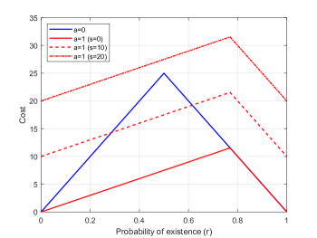
Figure 1: Cost $c\left(a\right)$ (for GOSPA) as a function of the probability $r$ of existence for $a=0$ and $a=1$, $p^{D}=0.7$, and $s\in\left\{0,10,20\right\}$.

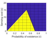
Figure 2: Optimal action (for GOSPA) as a function of the probability $r$ of existence and sensing cost $s$ for $p^{D}=0.6$ (left) and $p^{D}=0.7$ (right). Action $a=0$ is shown in blue and $a=1$ in yellow. As $p^{D}$ decreases, the size of the area to take action $1$ decreases because of a reduction in the value of making an observation.

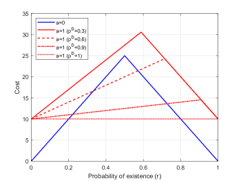
Figure 3: Cost $c\left(a\right)$ (for GOSPA) as a function of the probability $r$ of existence for $a=0$ and $a=1$, $s=10$, and $p^{D}\in\left\{0.3,0.6,0.9,1\right\}$.

Example 2.

This example analyses the effect of varying $p_{D}$ and $r$ to select the optimal action $\hat{a}$. We set $s=10$ and $p^{D}\in\left\{0.3,0.6,0.9,1\right\}$ and the resulting costs against $r$ are shown in Figure 3. For $p^{D}=1$, $c\left(1\right)$ is a constant equal to $s$, as there is no estimation error. Even for $p_{D}=1$, it is sometimes best not to take action 0 and not measure the target, if $r$ is sufficiently low or sufficiently high. As $p^{D}$ decreases, the slope of the first segment of $c\left(1\right)$ increases, and the range of values of $r$ in which it is best to take action $1$ decreases. For $p^{D}=0.3$, the best action is not to measure for all values of $r$. That is, the information we expect to obtain from measuring is not sufficient to compensate the sensing cost $s$. $\diamondsuit$

IV Analysis II: $N$ potential targets

We analyse the problem of deciding whether we should measure or not $N$ potential targets far away from each other. The prior is multi-Bernoulli with known target locations such that [4]

$$p\left(X\right) =\sum_{X_{1}\uplus...\uplus X_{N}=X}\prod_{i=1}^{N}f_{i}\left(X_{i}\right),$$ (15)

$$f_{i}\left(X\right) =\begin{cases}1-r_{i}&X=\emptyset\\ r_{i}\delta\left(x-\overline{x}_{i}\right)&X=\left\{x\right\}\\ 0&\mathrm{otherwise}\end{cases}$$ (16)

where $r_{i}$ is the probability of existence of the $i$-th Bernoulli and $\overline{x}_{i}$ is the location of the $i$-th Bernoulli component. All Bernoulli components are far from each other $d\left(\overline{x}_{i},\overline{x}_{j}\right)>c$ for $i\neq j$.

An action is represented as $a=\left[a_{1},...,a_{N}\right]$ where $a_{i}\in\left\{0,1\right\}$ with $a_{i}=0$ if we do not observe the $i$-th Bernoulli and $a_{i}=1$ if we observe it. We assume an additive sensor cost

$$s\left(a\right) =s\sum_{i=1}^{N}a_{i}$$ (17)

where $s$ is the cost of activating a single sensor.

In this analysis, under action $a=1$, we assume A1, A2 and

• A3 If $l\left(z|\overline{x}_{i}\right)>0$ then $l\left(z|\overline{x}_{j}\right)=0$ for $i\neq j.$

A3 implies that targets do not generate measurements in the areas of other targets.

We prove in Appendix B that the cost $c\left(a\right)$, with the GOSPA metric, is

$$c\left(a\right) =\sum_{i=1}^{N}c_{i}\left(a_{i}\right)$$ (18)

$$c_{i}\left(0\right) =\frac{c^{2}}{2}t\left(r_{i}\right)$$ (19)

$$c_{i}\left(1\right) =\frac{c^{2}}{2}t\left(\frac{r_{i}\left(1-p^{D}\right)}{1-r_{i}p^{D}}\right)\left(1-r_{i}p^{D}\right)+s.$$ (20)

The cost for GOSPA is additive over the Bernoulli components, which implies that the optimal actions are computed independently for each Bernoulli using (13) and (14).

For OSPA and UOSPA, there is not such a simplification. One should use Lemma 1 by evaluating all possible estimates and actions. In Appendix B, we provide more simplified expressions for 2 Bernoulli components, which are used for the following illustrative example.

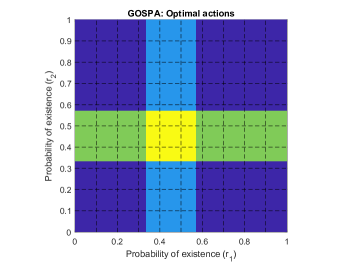
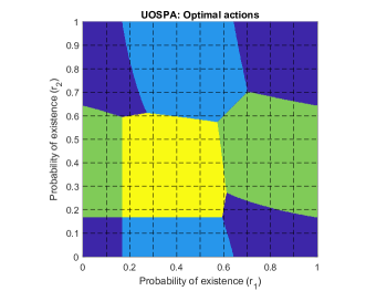
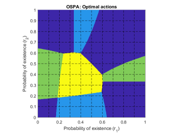
Figure 4: Optimal actions for GOSPA, UOSPA and OSPA metrics against the existence probabilities of two Bernoulli components. The colours for the optimal actions are: dark blue $a=\left(0,0\right)$, light blue $a=\left(1,0\right)$, green $a=\left(0,1\right)$ and yellow $a=\left(1,1\right)$. For GOSPA, the decision of whether to measure a target or not is taken independently of the other. For UOSPA and OSPA, there is coupling in the optimal actions.

Example 3.

This example analyses the optimal actions for $N=2$ Bernoulli components against the probability of existences. We use $c=10$, $p^{D}=0.6$ and $s=10$. The resulting optimal actions against $r_{1}$ and $r_{2}$ are shown in Figure 4. The optimal action is independent for each target using GOSPA. This is what is expected in most sensor systems observing non-overlapping, distant regions and whose sensor cost is additive. Note that the costs for each action for each target are similar to the ones in Figure 3. That is, we measure a given target if its probability of existence is not too low or too high, with optimal action indicated by (13) and (14).

When we use UOSPA and OSPA, there is influence of far-away independent targets on the optimal sensing mode for a sensor covering a different surveillance area. That is, for a given $r_{1}$, the sensing action $a_{1}$ for this target depends on $r_{2}$, the probability of existence of the other target. The choice of the optimal action is clearly counterintuitive for some choices of $r_{1}$ and $r_{2}$. For example, fixing $r_{2}=0.6$, the optimal action as a function of $r_{1}$ for both OSPA and UOSPA is shown in Figure 5. For OSPA, starting with $r_{1}=0$, we measure target 2. Then, as $r_{1}$ increases, we stop measuring target 2, even though nothing has changed related to target 2. If $r_{1}$ keeps increasing, we measure both targets. Then, we first stop measuring target 2, and then we stop measuring both targets. $\diamondsuit$

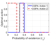
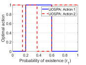
Figure 5: Optimal action as a function of $r_{1}$ fixing $r_{2}=0.6$ for OSPA and UOSPA. As opposed to GOSPA, a change in $r_{1}$ modifies the optimal action for both sensors.

The explanation of this behaviour of the optimal actions is that in order to minimise a metric-driven sensor management problem, we must consider the optimal estimators, as these minimise the corresponding error. UOSPA and OSPA optimal estimators suffer from spooky effect at a distance, in which the optimal estimation of a target is affected by the probability of existence of far-away independent targets. This effect translates to metric-driven sensor management by producing counterintuitive effects in the optimal actions. Though not included in this analysis, the complete OSPA metric [22] also suffers from spooky effect in optimal estimation, and entanglement of optimal actions in sensor management.

V Conclusion

This paper has presented two closed-form analyses for multi-target sensor management based on metrics. In a sensor management task that should be in principle separable for each sensor, only the GOSPA metric preserves this property. With GOSPA-driven sensor management, we aim to minimise localisation errors and the number of missed and false targets. This is an intuitive objective to drive sensor actions. This metric is also suitable to perform sensor management in large areas due to spatial separability.

On the contrary, even in separable sensor management problems, OSPA and UOSPA seek more complicated policies in which the optimal decision of a sensor is influenced by far away, independent potential targets. This paper therefore encourages the use of GOSPA for metric-driven sensor management for usual multiple target estimation tasks. The approach can also be extended to non-myopic sensor management with a metric for sets of trajectories [23], or the sum of the multi-target metric errors in a window of future time steps.

Appendix A

In this appendix, we provide the proofs of Analysis I in Section III. In particular, we prove the cost equations (10) and (11), and the optimal action equations, see (13) and (14).

The proof of (10) and (11) requires the following calculations: density of the measurement (3), posterior density (2), optimal estimate $\hat{X}\left(Z,a\right)$ and $\mathrm{MMSGOSPA}\left(Z,a\right)$, and finally evaluation of (8).

A-A Density of the measurement

We calculate $p\left(Z;a\right)$ in (3) for $a=1$ and $a=0$. For $a=0$,

$$p\left(Z;0\right) =\delta_{\emptyset}\left(Z\right).$$ (21)

For $a=1$, we have

$$p\left(Z;1\right) =\int f\left(Z|X;1\right)f\left(X\right)\delta X$$

$$=\left(1-r\right)f\left(Z|\emptyset;1\right)+rf\left(Z|\left\{\overline{x}\right\};1\right)$$

$$=\begin{cases}1-rp^{D}&Z=\emptyset\\ rp^{D}l\left(z|\overline{x}\right)&Z=\left\{z\right\}\\ 0&\mathrm{otherwise}\end{cases}$$ (22)

where we have used (9) and the properties of the measurement model. Note that $Z=\emptyset$ if the target does not exist, which occurs with probability $1-r$, or the target exists but is not detected, which occurs with probability $r\left(1-p^{D}\right)$.

A-B Posterior density

We calculate $p\left(X|Z;a\right)$ in (2) for $a=1$ and $a=0$. For $a=0$, the measurement $Z=\emptyset$ with probability one, and the posterior is equal to the prior

$$p\left(X|\emptyset;0\right) =p\left(X\right)$$

where $p\left(X\right)$ is given by (9). For $a=1$, we have two cases: $Z=\emptyset$ and $Z=\left\{z\right\}$. Applying Bayes’ rule, we obtain

$$p\left(X|\emptyset;1\right) =\frac{1}{1-r+r\left(1-p^{D}\right)}$$

$$\>\times\begin{cases}1-r&X=\emptyset\\ r\left(1-p^{D}\right)\delta\left(x-\overline{x}\right)&X=\left\{x\right\}\\ 0&\mathrm{otherwise}.\end{cases}$$

For $Z=\left\{z\right\}$, we obtain

$$p\left(X|\left\{z\right\};1\right) =\begin{cases}\delta\left(x-\overline{x}\right)&X=\left\{x\right\}\\ 0&\mathrm{otherwise}.\end{cases}$$

A-C Optimal estimate for GOSPA

The optimal estimate for GOSPA when the posterior is multi-Bernoulli with deterministic target state was calculated in [19]. We detect a target if its probability of existence is higher than 0.5, or misdetect it otherwise. We therefore have

$$\hat{X}\left(\emptyset,0\right) =\begin{cases}\emptyset&r<0.5\\ \left\{\overline{x}\right\}&\mathrm{otherwise}\end{cases}$$

$$\hat{X}\left(\emptyset,1\right) =\begin{cases}\emptyset&\frac{1-r}{1-rp^{D}}<0.5\\ \left\{\overline{x}\right\}&\mathrm{otherwise}\end{cases}$$

$$\hat{X}\left(\left\{z\right\},1\right) =\left\{\overline{x}\right\}.$$

A-D Action costs

We first calculate $\mathrm{MMSGOSPA}\left(Z,a\right)$ in (5), which corresponds to substituting the above optimal estimates into the MSGOSPA error, see [19, Eq.(5)], to obtain

$$\mathrm{MMSGOSPA}\left(\emptyset,0\right) =\frac{c^{2}}{2}t\left(r\right)$$ (23)

$$\mathrm{MMSGOSPA}\left(\emptyset,1\right) =\frac{c^{2}}{2}t\left(\frac{1-r}{1-rp^{D}}\right)$$

$$=\frac{c^{2}}{2}t\left(\frac{r\left(1-p^{D}\right)}{1-rp^{D}}\right)$$ (24)

$$\mathrm{MMSGOSPA}\left(\left\{z\right\},1\right) =0$$ (25)

where function $t\left(\cdot\right)$ is defined in (12).

We finish the proof of $c\left(0\right)$ and $c\left(1\right)$ ((10) and (11)) by substituting (21), (22) and (23)-(25) into (8).

A-E Optimal action

We proceed to calculate the optimal action $\hat{a}$. Function $t\left(\cdot\right)$ is a piece-wise function, which implies that (10) and (11) are piece-wise as well. Cost $c\left(0\right)$ has two segments $r<0.5$ and $r\geq 0.5$. The cost $c\left(1\right)$ has two segments

$$r<\frac{1}{2-p^{D}},\quad r\geq\frac{1}{2-p^{D}}.$$ (26)

We then have four segments in $r$ for which we should compute the minimum between $c\left(0\right)$ and $c\left(1\right)$. However, it is met that

$$\frac{1}{2-p^{D}} \geq 0.5$$ (27)

which implies that we actually have three regions of interest: $r<0.5$, $0.5\leq r<\frac{1}{2-p^{D}}$ and $r\geq\frac{1}{2-p^{D}}$.

A-E1 Region 1

For $r<0.5$, we have

$$c\left(0\right)=\frac{c^{2}}{2}r,\quad c\left(1\right)=\frac{c^{2}}{2}r\left(1-p^{D}\right)+s.$$ (28)

We take action 1 if $c\left(1\right)<c\left(0\right)$, which implies that

$$r >\frac{2s}{c^{2}p^{D}}.$$ (29)

A-E2 Region 2

For $0.5\leq r<\frac{1}{2-p^{D}}$, we have

$$c\left(0\right) =\frac{c^{2}}{2}\left(1-r\right)$$ (30)

$$c\left(1\right) =\frac{c^{2}}{2}r\left(1-p^{D}\right)+s.$$ (31)

We take action 1 if

$$r <\frac{\frac{c^{2}}{2}-s}{c^{2}\left(1-\frac{1}{2}p^{D}\right)}.$$ (32)

A-E3 Region 3

For $r_{1}>\frac{1}{2-p^{D}}$, we have

$$c\left(0\right) =\frac{c^{2}}{2}\left(1-r\right)$$ (33)

$$c\left(1\right) =\frac{c^{2}}{2}\left(1-r\right)+s.$$ (34)

The costs are the same for $s=0$. We never take action 1 for $s>0$. Putting all the results together, we finish the proof of the expression for the optimal action in (13) and (14).

Appendix B

In this appendix, we prove the results of Analysis II using GOSPA in Section IV.

B-A Density of the measurement

The density of the measurement set for action $a$ is

$$p\left(Z;a\right) =\sum_{Z_{1}\uplus...\uplus Z_{N}=Z}\prod_{i=1}^{N}p_{i}\left(Z_{i};a_{i}\right)$$ (35)

$$p_{i}\left(Z;1\right) =\begin{cases}1-r_{i}p^{D}&Z=\emptyset\\ r_{i}p^{D}l\left(z|\overline{x}_{i}\right)&Z=\left\{z\right\}\\ 0&\mathrm{otherwise}\end{cases}$$ (36)

$$p_{i}\left(Z;0\right) =\delta_{\emptyset}\left(Z\right).$$ (37)

These equations extend the results for one Bernoulli, and are analogous to the multi-Bernoulli filter prediction step [5].

B-B Posterior density

A measurement set $Z$ can be written as $Z=Z_{1}\uplus...\uplus Z_{N}$ where $Z_{i}=\emptyset$ if target located at $\overline{x}_{i}$ has not been detected and $Z_{i}=\left\{z\right\}$ with $z\sim l\left(\cdot|\overline{x}_{i}\right)$ if the target is detected. As targets are far away and $l\left(\cdot|\overline{x}_{i}\right)$ meets A3, given $Z$, we can recover $Z_{1},...,Z_{N}$ such that $Z=Z_{1}\uplus...\uplus Z_{N}$.

The posterior $p\left(X|Z;a\right)$ for $Z=Z_{1}\uplus...\uplus Z_{N}$ can be written as

$$p\left(X|Z;a\right) =\sum_{X_{1}\uplus...\uplus X_{N}=X}\prod_{i=1}^{N}p_{i}\left(X_{i}|Z_{i};a_{i}\right)$$ (38)

where, for $a_{i}=0$,

$$p_{i}\left(X_{i}|\emptyset;0\right) =p\left(X\right)$$ (39)

and, for $a_{i}=1$,

$$p_{i}\left(X_{i}|\emptyset;1\right) =\frac{1}{1-r_{i}+r_{i}\left(1-p^{D}\right)}$$

$$\>\times\begin{cases}1-r_{i}&X=\emptyset\\ r_{i}\left(1-p^{D}\right)\delta\left(x-\overline{x}_{i}\right)&X=\left\{x\right\}\\ 0&\mathrm{otherwise}.\end{cases}$$ (40)

For $Z=\left\{z\right\}$, we obtain

$$p_{i}\left(X_{i}|\left\{z\right\};1\right) =\begin{cases}\delta\left(x-\overline{x}_{i}\right)&X=\left\{x\right\}\\ 0&\mathrm{otherwise}.\end{cases}$$ (41)

This result can be obtained from the Poisson multi-Bernoulli mixture update [5, 6] and the multi-Bernoulli mixture update [24]. Due to A3, only the local hypotheses that link the $i$-th Bernoulli with $Z_{i}\neq\emptyset$ or with $Z_{i}=\emptyset$ exist.

B-C Optimal estimate and cost for GOSPA

The estimate that minimises the MSGOSPA error for measurement $Z$ and action $a$ is [19]

$$\hat{X}\left(Z,a\right) =\hat{X_{1}}\left(Z_{1},a_{1}\right)\cup...\cup\hat{X}_{N}\left(Z_{N},a_{N}\right)$$

$$\hat{X}_{i}\left(\emptyset,0\right) =\begin{cases}\emptyset&r_{i}<0.5\\ \left\{\overline{x}_{i}\right\}&\mathrm{otherwise}\end{cases}$$

$$\hat{X}_{i}\left(\emptyset,1\right) =\begin{cases}\emptyset&\frac{1-r_{i}}{1-r_{i}p^{D}}<0.5\\ \left\{\overline{x}_{i}\right\}&\mathrm{otherwise}\end{cases}$$

$$\hat{X}_{i}\left(\left\{z\right\},1\right) =\left\{\overline{x}_{i}\right\}.$$

The MSGOSPA error is additive for each Bernoulli [19]. Then, the cost $c\left(a\right)$ for GOSPA becomes (18) and (20), where $t\left(\cdot\right)$ is defined in (12) and we have used the result obtained for one Bernoulli component.

Appendix C

The expressions for the optimal estimate and action cost for general $N$ for OSPA and UOSPA are more complex than for GOSPA. We develop the expression (8) to be able to obtain the optimal action for the case $N=2$. We focus on the OSPA case, and then point out how to extend it to UOSPA.

C-A Minimum mean square error

We denote a possible (optimal) estimate of the set of targets using existence variables $\hat{e}_{1}$ and $\hat{e}_{2}$, where $\hat{e}_{i}=1$ if the $i$-th Bernoulli component is detected and zero otherwise. The estimated set is

$$\hat{X} =\left\{\overline{x}_{i}:\hat{e}_{i}=1,\,i\in\left\{1,2\right\}\right\}.$$ (42)

The MSOSPA error of this estimate when the posterior existence of the Bernoullis are $r_{1}$ and $r_{2}$ is [19]

$$\mathrm{MSOSPA}\left(r_{1},r_{2},\hat{e}_{1},\hat{e}_{2}\right)$$

$$=\begin{cases}c^{2}\left(1-\sum_{i=1}^{2}\left[\hat{e}_{i}r_{i}\sum_{n=0}^{1}\frac{\rho_{-i}\left(n\right)}{\max\left(n+1,\hat{n}\right)}\right]\right)&\hat{n}>0\\ c^{2}\left(1-\rho\left(0\right)\right)&\hat{n}=0\end{cases}$$ (43)

where $\hat{n}=\hat{e}_{1}+\hat{e}_{2}$ is the number of detected targets, $\rho\left(\cdot\right)$ is the cardinality distribution of the multi-Bernoulli density (15) and $\rho_{-i}\left(\cdot\right)$ is the cardinality distribution of the multi-Bernoulli density without the $i$-th Bernoulli component.

The resulting MMSOSPA is

$$\mathrm{MMSOSPA}\left(r_{1},r_{2}\right) =\min_{\hat{e}_{1},\hat{e}_{2}}\mathrm{MSOSPA}\left(r_{1},r_{2},\hat{e}_{1},\hat{e}_{2}\right)$$

where the minimum can be computed by evaluating the four possible $\left(\hat{e}_{1},\hat{e}_{2}\right)$.

We proceed to compute the factor in (7) corresponding to OSPA for each action, which is denoted as

$$c_{m}\left(a\right) =\int\mathrm{MMSOSPA}\left(Z,a\right)p\left(Z;a\right)\delta Z.$$ (44)

It should be noted that with a slight abuse of notation we use $\mathrm{MMSOSPA}\left(r_{1},r_{2}\right)$ and $\mathrm{MMSOSPA}\left(Z,a\right)$ to denote the MMSOSPA as a function of the Bernoulli existences involved in the calculation, or as a function of $Z$ and $a$. To compute (44), we need the density of the measurement and the posterior, which are given by (35) and (38), respectively.

C-B Action $a=\left[0,0\right]$

The density of the measurement is $f\left(Z|\left[0,0\right]\right)=\delta_{\emptyset}\left(Z\right)$ and the posterior is equal to the prior. Therefore,

$$c_{m}\left(\left[0,0\right]\right) =\mathrm{MMSOSPA}\left(r_{1},r_{2}\right).$$ (45)

C-C Action $a=\left[1,0\right]$

In this case, set $Z_{2}=\emptyset$ with probability one. Therefore, the integral over $Z$ in (44) is over a Bernoulli component with density (36). Then, we have

$$c_{m}\left(\left[1,0\right]\right) =\left(1-r_{1}p^{D}\right)\mathrm{MMSOSPA}\left(\frac{r_{1}\left(1-p^{D}\right)}{1-r_{1}p^{D}},r_{2}\right)$$

$$+r_{1}p^{D}\mathrm{MMSOSPA}\left(1,r_{2}\right).$$ (46)

The cost for action $a=\left[0,1\right]$ is analogous to (46) but interchanging $r_{1}$ and $r_{2}$.

C-D Action $a=\left[1,1\right]$

The density of the measurement is multi-Bernoulli with probabilities of existence $r_{1}p^{D}$ and $r_{2}p^{D}$. We integrate over the four possible cases (detection and misdetection of the two targets)

$$c_{m}\left(\left[1,1\right]\right) =\left(1-r_{1}p^{D}\right)\left(1-r_{2}p^{D}\right)$$

$$\times\mathrm{MMSOSPA}\left(\frac{r_{1}\left(1-p^{D}\right)}{1-r_{1}p^{D}},\frac{r_{2}\left(1-p^{D}\right)}{1-r_{2}p^{D}}\right)$$

$$+r_{1}p^{D}\left(1-r_{2}p^{D}\right)\mathrm{MMSOSPA}\left(1,\frac{r_{2}\left(1-p^{D}\right)}{1-r_{2}p^{D}}\right)$$

$$+r_{2}p^{D}\left(1-r_{1}p^{D}\right)\mathrm{MMSOSPA}\left(\frac{r_{1}\left(1-p^{D}\right)}{1-r_{1}p^{D}},1\right).$$

We can now compute the optimal action using Lemma 1. The UOSPA costs are obtained by using the MSUOSPA [19, Eq. (6)] instead MSOSPA in (43).

References

- [1] C. M. Kreucher, A. O. Hero III, K. D. Kastella, and M. R. Morelande, “An information-based approach to sensor management in large dynamic networks,” Proc. of the IEEE, vol. 95, no. 5, pp. 978–999, May 2007.
- [2] A. O. Hero III, D. A. Castañón, D. Cochran, and K. Kastella, Foundations and Applications of Sensor Management. Springer, 2008.
- [3] S. Thrun, W. Burgard, and D. Fox, Probabilistic Robotics. MIT Press, 2005.
- [4] R. P. S. Mahler, Advances in Statistical Multisource-Multitarget Information Fusion. Artech House, 2014.
- [5] J. L. Williams, “Marginal multi-Bernoulli filters: RFS derivation of MHT, JIPDA and association-based MeMBer,” IEEE Trans. Aeros. and Elect. Syst., vol. 51, no. 3, pp. 1664–1687, July 2015.
- [6] A. F. García-Fernández, J. L. Williams, K. Granström, and L. Svensson, “Poisson multi-Bernoulli mixture filter: direct derivation and implementation,” IEEE Trans. Aeros. and Elect. Syst., vol. 54, no. 4, pp. 1883–1901, Aug. 2018.
- [7] P. Boström-Rost, D. Axehill, and G. Hendeby, “Sensor management for search and track using the Poisson multi-Bernoulli mixture filter,” IEEE Trans. Aeros. and Elect. Syst., 2021.
- [8] M. Hernandez, “Performance bounds for target tracking: computationally efficient formulations and associated applications,” in Integrated tracking, classification and sensor management, M. Mallick, V. Krishnamurthy, and B. N. Vo, Eds., 2013.
- [9] R. Tharmarasa, T. Kirubarajan, M. L. Hernandez, and A. Sinha, “PCRLB-based multisensor array management for multitarget tracking,” IEEE Trans. Aeros. and Elect. Syst., vol. 43, no. 2, pp. 539–555, April 2007.
- [10] K. L. Bell, C. J. Baker, G. E. Smith, J. T. Johnson, and M. Rangaswamy, “Cognitive radar framework for target detection and tracking,” IEEE Journal of Selected Topics in Signal Processing, vol. 9, no. 8, pp. 1427–1439, Dec. 2015.
- [11] E. H. Aoki, A. Bagchi, P. Mandal, and Y. Boers, “A theoretical look at information-driven sensor management criteria,” in International Conference on Information Fusion, 2011, pp. 1180–1187.
- [12] B. Ristic, B.-N. Vo, and D. Clark, “A note on the reward function for PHD filters with sensor control,” IEEE Trans. Aeros. and Elect. Syst., vol. 47, no. 2, pp. 1521–1529, April 2011.
- [13] M. Beard, B.-T. Vo, B.-N. Vo, and S. Arulampalam, “Void probabilities and Cauchy-Schwarz divergence for generalized labeled multi-Bernoulli models,” IEEE Transactions on Signal Processing, vol. 65, no. 19, pp. 5047–5061, Oct. 2017.
- [14] D. Schuhmacher and A. Xia, “A new metric between distributions of point processes,” Advances in Applied Probability, vol. 40, no. 3, pp. 651–672, Sep. 2008.
- [15] D. Schuhmacher, B.-T. Vo, and B.-N. Vo, “A consistent metric for performance evaluation of multi-object filters,” IEEE Transactions on Signal Processing, vol. 56, no. 8, pp. 3447–3457, Aug. 2008.
- [16] A. K. Gostar, R. Hoseinnezhad, A. Bab-Hadiashar, and F. Papi, “OSPA-based sensor control,” in International Conference on Control, Automation and Information Sciences, 2015, pp. 214–218.
- [17] O. E. Drummond and B. E. Fridling, “Ambiguities in evaluating performance of multiple target tracking algorithms,” in Proceedings of the SPIE conference, 1992, pp. 326–337.
- [18] A. S. Rahmathullah, A. F. García-Fernández, and L. Svensson, “Generalized optimal sub-pattern assignment metric,” in 20th International Conference on Information Fusion, 2017, pp. 1–8.
- [19] A. F. García-Fernández and L. Svensson, “Spooky effect in optimal OSPA estimation and how GOSPA solves it,” in Proceedings on the 22nd International Conference on Information Fusion, 2019.
- [20] L. Úbeda-Medina, “Robust techniques for multiple target tracking and fully adaptive radar,” Ph.D. dissertation, Universidad Politécnica de Madrid, 2018. [Online]. Available: http://oa.upm.es/53209/
- [21] P. Barrios, M. Adams, K. Leung, F. Inostroza, G. Naqvi, and M. E. Orchard, “Metrics for evaluating feature-based mapping performance,” IEEE Transactions on Robotics, vol. 33, no. 1, pp. 198–213, Feb. 2017.
- [22] T. Vu, “A complete optimal subpattern assignment (COSPA) metric,” in 23rd International Conference on Information Fusion, 2020, pp. 1–8.
- [23] A. F. García-Fernández, A. S. Rahmathullah, and L. Svensson, “A metric on the space of finite sets of trajectories for evaluation of multi-target tracking algorithms,” IEEE Transactions on Signal Processing, vol. 68, pp. 3917–3928, 2020.
- [24] A. F. García-Fernández, Y. Xia, K. Granström, L. Svensson, and J. L. Williams, “Gaussian implementation of the multi-Bernoulli mixture filter,” in Proceedings of the 22nd International Conference on Information Fusion, 2019.