Abstract

Attention based models such as Transformers involve pairwise interactions between data points, modeled with a learnable attention matrix. Importantly, this attention matrix is normalized with the SoftMax operator, which makes it row-wise stochastic. In this paper, we propose instead to use Sinkhorn’s algorithm to make attention matrices doubly stochastic. We call the resulting model a Sinkformer. We show that the row-wise stochastic attention matrices in classical Transformers get close to doubly stochastic matrices as the number of epochs increases, justifying the use of Sinkhorn normalization as an informative prior. On the theoretical side, we show that, unlike the SoftMax operation, this normalization makes it possible to understand the iterations of self-attention modules as a discretized gradient-flow for the Wasserstein metric. We also show in the infinite number of samples limit that, when rescaling both attention matrices and depth, Sinkformers operate a heat diffusion. On the experimental side, we show that Sinkformers enhance model accuracy in vision and natural language processing tasks. In particular, on 3D shapes classification, Sinkformers lead to a significant improvement.

1 Introduction

The Transformer (Vaswani et al.,, 2017), an architecture that relies entirely on attention mechanisms (Bahdanau et al.,, 2014), has achieved state of the art empirical success in natural language processing (NLP) (Brown et al.,, 2020; Radford et al.,, 2019; Wolf et al.,, 2019) as well as in computer vision (Dosovitskiy et al.,, 2020; Zhao et al.,, 2020; Zhai et al.,, 2021; Lee et al.,, 2019). As the key building block of the Transformer, the self-attention mechanism takes the following residual form (Yun et al.,, 2019) given a $n$-sequence $(x_{1},x_{2},...,x_{n})$, embedded in dimension $d$:

$$x_{i}\leftarrow x_{i}+\sum^{n}_{j=1}K^{1}_{i,j}W_{V}x_{j},$$ (1)

where ${K^{1}}\coloneqq\texttt{SoftMax}(C)$ with $C_{i,j}\coloneqq({W_{Q}x_{i}})^{\top}{W_{K}x_{j}}$ $=x_{i}^{\top}W_{Q}^{\top}W_{K}x_{j}$. Here, $W_{Q},W_{K}\in\mathbb{R}^{m\times d}$ and $W_{V}\in\mathbb{R}^{d\times d}$ are the query, key and value matrices. The SoftMax operator can be seen as a normalization of the matrix $K^{0}\coloneqq\exp(C)$ as follows: $K^{1}_{ij}\coloneqq K^{0}_{ij}/\sum_{l=1}^{n}K^{0}_{il}$ for all $i$ and $j$. Importantly, the matrix $K^{1}$ is row-wise stochastic: its rows all sum to $1$.

In this work, we propose to take the normalization process further by successively normalizing the rows and columns of $K^{0}$. This process is known to provably converge to a doubly stochastic matrix (i.e., whose rows and columns both sum to $1$) and is called Sinkhorn’s algorithm (Sinkhorn,, 1964; Cuturi,, 2013; Peyré et al.,, 2019). We denote the resulting doubly stochastic matrix $K^{\infty}$. Intuitively, such a normalization relies on a democratic principle where all points are matched one to another with different degrees of intensity, so that more interactions are considered than with the SoftMax normalization, as shown in Figure 1.

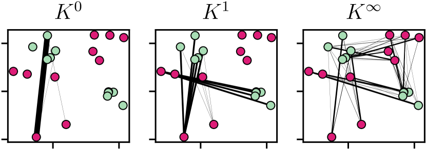
Figure 1: Illustration of the different normalizations of attention matrices. We form two point clouds $(W_{Q}x_{i})_{1\leq i\leq 10}$ (green) and $(W_{K}x_{j})_{1\leq i\leq 10}$ (red). For $k\in\{0,1,\infty\}$, the width of the line connecting $x_{i}$ to $x_{j}$ is $K^{k}_{i,j}$. We only display connections with $K^{k}_{i,j}\geq 10^{-12}$. For $K^{0}$, one interaction dominates. For $K^{1}$ (SoftMax), one cluster is ignored. For $K^{\infty}$ (Sinkhorn), all points are involved in an interaction.

We call our Transformer variant where the SoftMax is replaced by Sinkhorn a Sinkformer. Since Sinkhorn’s first iteration coincides exactly with the SoftMax, Sinkformers include Transformers as a special case. Our modification is differentiable, easy to implement using deep learning libraries, and can be executed on GPUs for fast computation. Because the set of row-wise stochastic matrices contains the set of doubly stochastic matrices, the use of doubly stochastic matrices can be interpreted as a prior. On the experimental side, we confirm that doubly stochastic attention leads to better accuracy in several learning tasks. On the theoretical side, doubly stochastic matrices also give a better understanding of the mathematical properties of self-attention maps.

To summarize, we make the following contributions.

• We show empirically that row-wise stochastic matrices seem to converge to doubly stochastic matrices during the learning process in several classical Transformers (Figure 2). Motivated by this finding, we then introduce the Sinkformer, an extension of the Transformer in which the SoftMax is replaced by the output of Sinkhorn’s algorithm. In practice, our model is parametrized by the number of iterations in the algorithm, therefore interpolating between the Transformer and the Sinkformer.

• On the theoretical side, we show that Transformers and Sinkformers can be viewed as models acting on discrete distributions, and we show under a symmetry assumption that Sinkformers can be seen in the infinite depth limit as a Wasserstein gradient flow for an energy minimization (Proposition 2). We also show that the classical Transformer with the SoftMax operator cannot be interpreted as such a flow (Proposition 3). To the best of our knowledge, this is the first time such a connection is established. We also prove that in the infinite number of particles limit (when $n$ goes to infinity), the iterations of Sinkformers converge to the heat equation (Theorem 1), while the corresponding equation for Transformers is nonlinear and nonlocal (Proposition 4).

• On the experimental side, we show that Sinkformers lead to a significant accuracy gain compared to Transformers on the ModelNet 40 3D shapes classification task. We then demonstrate better performance of Sinkformers on the NLP IMDb dataset for sentiment analysis and IWSLT’14 German to English neural machine translation tasks. Sinkformers also achieve a better accuracy than Vision Transformers on image classification tasks. Therefore, the proposed method is capable of enhancing the performance of transformers in a wide range of applications.

2 Background and related work

Transformers.

Proposed by Vaswani et al., (2017), the Transformer is a fully attention-based architecture. Originally designed to process sequences for natural language processing (NLP), many variants have since been developed such as Vision Transformers (Dosovitskiy et al.,, 2020; Zhai et al.,, 2021), Set Transformers (Lee et al.,, 2019) or Point Cloud Transformers (Zhao et al.,, 2020). The Transformer and its variants are based on an encoder-decoder structure, where the decoder can have a more or less complex form. The encoder is fully self-attention based. After embedding and concatenating with positional encoding the original input sequence, the encoder uses a series of residual blocks that iterates relation (1) followed by a feed forward neural network applied to each $x_{i}$ independently. In its most complex form such as in neural machine translation, the decoder combines a self-attention based mechanisms and a cross attention one, meaning that it is given access to the encoder via another multi-head attention block.

Sinkhorn and Attention.

To the best of our knowledge, using Sinkhorn’s algorithm in Transformers has been done once in a different context (Tay et al.,, 2020). The authors propose to learn efficient and sparse attention using a differentiable algorithm for sorting and rearranging elements in the input sequence. For this purpose, they introduce a sorting network to generate a doubly-stochastic matrix (that can be seen as a relaxed version of a permutation matrix) and use it to sort the sequence in a differentiable fashion. Mialon et al., (2021) propose an embedding for sets of features in $\mathbb{R}^{d}$ based on Sinkhorn’s algorithm, by using the regularized optimal transport plan between data points and a reference set. Niculae et al., (2018) use doubly stochastic attention matrices in LSTM-based encoder-decoder networks but they use Frank-Wolfe or active set methods to compute the attention matrix. None of these works use Sinkhorn on self-attention maps in Transformers and provide its theoretical analysis, as we do.

Impact of bi-normalization.

Theoretical properties of kernels $\mathcal{K}$, which attention is an instance of, can also be studied through the operator $f\mapsto f-\mathcal{K}f$. Bi-normalization of kernels over manifolds have already been studied in the literature, on uniform measures (Singer,, 2006), weighted measures (Hein et al.,, 2007) and in a more general setup with associated diffusion operators (Ting et al.,, 2011). Milanfar, (2013) proposes to approximate smoothing operators by doubly stochastic matrices using Sinkhorn’s updates, leading to better performance in data analysis and signal processing. Importantly, the works of Marshall and Coifman, (2019) and Wormell and Reich, (2021) exactly introduce a normalization that is based on Sinkhorn’s algorithm. They prove that this method models a Langevin diffusion and leads to the approximation of a symmetric operator. They also show that convergence to this operator is faster with Sinkhorn normalization than with the SoftMax normalization. In section 5, we adopt a similar point of view with a parametrized cost and show that different normalizations result in different partial differential equations (PDEs) in the infinite number of particles limit.

Infinite depth limit.

Studying deep residual neural networks (ResNets) (He et al.,, 2016) in the infinitesimal step-size regime (or infinite depth limit) has recently emerged as a new framework for analyzing their theoretical properties. The ResNet equation

$$x_{i}\leftarrow x_{i}+T(x_{i})$$ (2)

can indeed be seen as a discretized Euler scheme with unit step size of the ordinary differential equation (ODE) $\dot{x_{i}}=T(x_{i})$ (Weinan,, 2017; Chen et al.,, 2018; Teh et al.,, 2019; Sun et al.,, 2018; Weinan et al.,, 2019; Lu et al.,, 2018; Ruthotto and Haber,, 2019; Sander et al.,, 2021). In section 4, we adopt this point of view on residual attention layers in order to get a better theoretical understanding of attention mechanisms. This is justified by the fact that, for instance, GPT-3 (Brown et al.,, 2020) has 96 layers.

Neural networks on measures.

The self-attention mechanism (1) acts on sets $\{x_{i}\}_{i}$ where the ordering of the elements does not matter. An equivalent way to model such invariant architectures is to consider them as acting on probability measures or point clouds of varying cardinality (De Bie et al.,, 2019; Vuckovic et al.,, 2021; Zweig and Bruna,, 2021). Specifically, a collection of points $(x_{i})_{1\leq i\leq n}$, where $x_{i}\in\mathbb{R}^{d}$, can also be seen as a discrete measure on $\mathbb{R}^{d}$: $\mu\coloneqq\frac{1}{n}\sum_{i=1}^{n}\delta_{x_{i}}\in\mathcal{M}(\mathbb{R}^{d})$, where $\mathcal{M}(\mathbb{R}^{d})$ is the set of probability measures on $\mathbb{R}^{d}$. A map $T_{\mu}$ then acts on $\mu$ through $F(\mu)\coloneqq\frac{1}{n}\sum_{i=1}^{n}\delta_{T_{\mu}(x_{i})}$. One notable interest of such a point of view is to consider the evolution of non ordered sets of points. Another is to consider the mean field (or large sample) limit, that is when $n\to\infty$, to conduct theoretical analysis (Zweig and Bruna,, 2021) as when analyzing the SGD properties in the mean-field limit (Song et al.,, 2018).

3 Sinkformers

We now introduce Sinkformers, a modification of any Transformer by replacing the SoftMax operator in the attention modules by Sinkhorn’s algorithm.

Attention matrices during training.

In Transformers, attention matrices are row-wise stochastic. A natural question is how the sum over columns evolve during training. On $3$ different models and $3$ different learning tasks, we calculated the sum over columns of attention matrices in Transformers. We find out that the learning process makes the attention matrices more and more doubly stochastic, as shown in Figure 2.

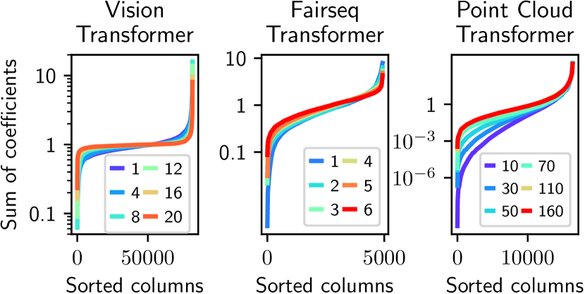
Figure 2: Sum over columns of attention matrices at different training epochs (color) when training, from left to right, a ViT on MNIST (section 6.4), a fairseq Transformer on IWSLT’14 (section 6.3), and a Point Cloud Transformer on Model Net 40 (section 6.1). The majority of columns naturally sum closely to $1$.

Thus, row-wise stochastic attention matrices seem to approach doubly stochastic matrices during the learning process in classical Transformers. Therefore, it seems natural to impose double stochasticity as a prior and study theoretically and experimentally the resulting model. A process to obtain such matrices which extends the SoftMax is Sinkhorn’s algorithm.

Sinkhorn’s algorithm.

Given a matrix $C\in\mathbb{R}^{n\times n}$, and denoting $K^{0}\in\mathbb{R}^{n\times n}$ such that $K^{0}=\exp(C)$, Sinkhorn’s algorithm (Sinkhorn,, 1964; Cuturi,, 2013; Peyré et al.,, 2019) iterates, starting from $K^{0}$:

$$K^{l+1}=\left\{\begin{array}[]{r@{\hspace{1mm}}l}\hskip 2.84526pt&N_{R}(K^{l})\quad\text{if $l$ is even}\\ \hskip 2.84526pt&N_{C}(K^{l})\quad\text{if $l$ is odd},\end{array}\right.$$ (3)

where $N_{R}$ and $N_{C}$ correspond to row-wise and column-wise normalizations: $(N_{R}(K))_{i,j}\coloneqq\frac{K_{i,j}}{\sum_{l=1}^{n}K_{i,l}}$ and $(N_{C}(K))_{i,j}\coloneqq\frac{K_{i,j}}{\sum_{l=1}^{n}K_{l,j}}$. We denote the resulting scaled matrix limit $K^{\infty}\coloneqq\texttt{Sinkhorn}(C)$. Note that it is doubly stochastic in the sense that $K^{\infty}\mathbb{1}_{n}=\mathbb{1}_{n}$ and ${K^{\infty}}^{\top}\mathbb{1}_{n}=\mathbb{1}_{n}$. The operations in (3) are perfectly suited for being executed on GPUs (Charlier et al.,, 2021; Cuturi,, 2013).

Sinkformers.

For simplicity, we consider a one head attention block that iterates equation (1). Note that $K^{1}\coloneqq\texttt{SoftMax}(C)$ is precisely the output of Sinkhorn’s algorithm (3) after $1$ iteration. In this paper, we propose to take Sinkhorn’s algorithm several steps further until it approximately converges to a doubly stochastic matrix $K^{\infty}$. This process can be easily implemented in practice, simply by plugging Sinkhorn’s algorithm into self-attention modules in existing architectures, without changing the overall structure of the network. We call the resulting drop-in replacement of a Transformer a Sinkformer. It iterates

$$x_{i}\leftarrow x_{i}+\sum^{n}_{j=1}K^{\infty}_{i,j}W_{V}x_{j}.$$ (4)

In the next two sections 4 and 5, we investigate the theoretical properties of Sinkformers. We exhibit connections with energy minimization in the space of measures and the heat equation, thereby proposing a new framework for understanding attention mechanisms. All our experiments are described in Section 6 and show the benefits of using Sinkformers in a wide variety of applications.

Computational cost and differentiation.

Turning a Transformer into a Sinkformer simply relies on replacing the SoftMax by Sinkhorn, i.e., substituting $K^{1}$ with $K^{\infty}$. In practice, we use a finite number of Sinkhorn iterations and therefore use $K^{l}$, where $l$ is large enough so that $K^{l}$ is almost doubly stochastic. Doing $l$ iterations of Sinkhorn takes $l$ times longer than the SoftMax. However, this is not a problem in practice because Sinkhorn is not the main computational bottleneck and because only a few iterations of Sinkhorn are sufficient (typically $3$ to $5$) to converge to a doubly stochastic matrix. As a result, the practical training time of Sinkformers is comparable to regular Transformers, as detailed in our experiments.

Sinkhorn is perfectly suited for backpropagation (automatic differentiation), by differentiating through the operations of (3). The Jacobian of an optimization problem solution can also be computed using the implicit function theorem (Griewank and Walther,, 2008; Krantz and Parks,, 2012; Blondel et al.,, 2021) instead of backpropagation if the number of iterations becomes a memory bottleneck. Together with Sinkhorn, implicit differentiation has been used by Luise et al., (2018) and Cuturi et al., (2020).

Invariance to the cost function.

Recall that in practice one has $C_{i,j}=({W_{Q}x_{i}})^{\top}{W_{K}x_{j}}$. An important aspect of Sinkformers is that their output is unchanged if the cost is modified with non interacting terms, as the next proposition shows.

Proposition 1.

Let $C\in\mathbb{R}^{n\times n}$. Consider, for $(f,g)\in\mathbb{R}^{n}\times\mathbb{R}^{n}$ the modified cost function $\tilde{C}_{i,j}\coloneqq C_{i,j}+f_{i}+g_{j}$. Then $\texttt{Sinkhorn}(C)=\texttt{Sinkhorn}(\tilde{C})$.

A proof is available in Appendix A. A consequence of this result is that one can consider the cost $\tilde{C}_{i,j}\coloneqq-\frac{1}{2}\|{W_{Q}x_{i}}-{W_{K}x_{j}}\|^{2}$ instead of $C_{i,j}=({W_{Q}x_{i}})^{\top}{W_{K}x_{j}}$, without affecting $K^{\infty}$. A Transformer using the cost $\tilde{C}$ is referred to as L2 self-attention, and is Lipschitz under some assumptions (Kim et al.,, 2021) and can therefore be used as an invertible model (Behrmann et al.,, 2019). For instance, we use $\tilde{C}$ in Proposition 4.

4 Attention and gradient flows

In this section, we make a parallel between self-attention modules in Sinkformers and gradient flows in the space of measures. We denote $\mathcal{M}(\mathbb{R}^{d})$ the probability measures on $\mathbb{R}^{d}$ and $\mathcal{C}(\mathbb{R}^{d})$ the continuous functions on $\mathbb{R}^{d}$. We denote $\nabla$ the gradient operator, $\mathrm{div}$ the divergence, and $\Delta$ the Laplacian, that is $\Delta=\mathrm{div}(\nabla)$.

Residual maps for attention.

We consider a one-head attention block operating with different normalizations. We consider the continuous counterparts of the attention matrices seen in the previous section. We denote $c(x,x^{\prime})\coloneqq{(W_{Q}x)}^{\top}W_{K}x^{\prime}$ and $k^{0}\coloneqq\exp(c)$. For some measure $\mu\in\mathcal{M}(\mathbb{R}^{d})$, we define the SoftMax operator on the cost $c$ by $k^{1}(x,x^{\prime})=\texttt{SoftMax}(c)(x,x^{\prime})\coloneqq\frac{k^{0}(x,x^{\prime})}{\int k^{0}(x,y)d\mu(y)}$. Similarly, we define Sinkhorn’s algorithm as the following iterations, starting from $k^{0}=\exp(c)$:

$$k^{l+1}(x,x^{\prime})=\left\{\begin{array}[]{r@{\hspace{2mm}}l}\hskip 5.69054pt&\frac{k^{l}(x,x^{\prime})}{\int k^{l}(x,y)d\mu(y)}\quad\text{if $l$ is even}\\ \hskip 5.69054pt&\frac{k^{l}(x,x^{\prime})}{\int k^{l}(y,x)d\mu(y)}\quad\text{if $l$ is odd}.\end{array}\right.$$ (5)

We denote $k^{\infty}\coloneqq\texttt{Sinkhorn}(c)$ the resulting limit. Note that if $\mu$ is a discrete measure supported on a $n$ sequence of particles $(x_{1},x_{2},...,x_{n})$, $\mu=\frac{1}{n}\sum_{i=1}^{n}\delta_{x_{i}}$, then for all $(i,j)$, $k^{0}(x_{i},x_{j})=K^{0}_{i,j}$, $k^{1}(x_{i},x_{j})=K^{1}_{i,j}$ and $k^{\infty}(x_{i},x_{j})=K^{\infty}_{i,j}$, so that $k^{0}$, $k^{1}$ and $k^{\infty}$ are indeed the continuous equivalent of the matrices $K^{0}$, $K^{1}$ and $K^{\infty}$ respectively.

Infinitesimal step-size regime.

In order to better understand the theoretical properties of attention matrices in Transformers and Sinkformers, we omit the feed forward neural networks acting after each attention block. We consider a succession of attention blocks with tied weights between layers and study the infinite depth limit where the output is given by solving a neural ODE (Chen et al.,, 2018). In this framework, iterating the Transformer equation (1), the ResNet equation (2) and the Sinkformer equation (4) corresponds to a Euler discretization with step-size $1$ of the ODEs

$$\dot{x}_{i}=T_{\mu}(x_{i})~{}\text{for all }i,$$ (6)

where $x_{i}(t)$ is the position of $x_{i}$ at time $t$. For an arbitrary measure $\mu\in\mathcal{M}(\mathbb{R}^{d})$, these ODEs can be equivalently written as a continuity equation (Renardy and Rogers,, 2006)

$$\partial_{t}\mu+\mathrm{div}(\mu T_{\mu})=0.$$ (7)

When $T_{\mu}$ is defined by the ResNet equation (2), $T_{\mu}=T$ does not depend on $\mu$. It defines an advection equation where the particles do not interact and evolve independently. When $T_{\mu}$ is defined by the Transformer equation (1) or Sinkformer equation (4), $T_{\mu}$ has a dependency in $\mu$ and the particles interact: the local vector field depends on the position of the other particles. More precisely we have in this case $T^{1}_{\mu}(x)=\int k^{1}(x,x^{\prime})W_{V}x^{\prime}d\mu(x^{\prime})$ for the Transformer and $T^{\infty}_{\mu}(x)=\int k^{\infty}(x,x^{\prime})W_{V}x^{\prime}d\mu(x^{\prime})$ for the Sinkformer. It is easily seen that when $\mu$ is discrete we recover the operators in equation (1) and (4).

Wasserstein gradient flows.

A particular case of equation (7) is when $T_{\mu}$ is a gradient with respect to the Wasserstein metric $W_{2}$. Let $\mathcal{F}$ be a function on $\mathcal{M}(\mathbb{R}^{d})$. As is standard, we suppose that $\mathcal{F}$ admits a first variation at all $\mu$: there exists a function $\frac{\delta\mathcal{F}}{\delta\mu}(\mu)$ such that $\frac{d}{d\varepsilon}\mathcal{F}(\mu+\varepsilon\rho)_{|\varepsilon=0}=\int\frac{\delta\mathcal{F}}{\delta\mu}(\mu)d\rho$ for every perturbation $\rho$ (Santambrogio,, 2017). The Wasserstein gradient of $\mathcal{F}$ at $\mu$ is then $\nabla_{W}\mathcal{F}(\mu)\coloneqq\nabla(\frac{\delta\mathcal{F}}{\delta\mu}(\mu))$. The minimization of $\mathcal{F}$ on the space of measures corresponds to the PDE (7) with $T_{\mu}=-\nabla_{W}\mathcal{F}(\mu)$. This PDE can be interpreted as ruling the evolution of the measure $\mu$ of particles initially distributed according to some measure $\mu_{0}$, for which the positions $x(t)$ follow the flow $\dot{x}=-\nabla_{W}\mathcal{F}(\mu)(x)$, that minimizes the global energy $\mathcal{F}$. It corresponds to a steepest descent in Wasserstein space (Jordan et al.,, 1998). In Proposition 2, we show in the symmetric kernel case that Sinkformers correspond to a Wasserstein gradient flow for some functional $\mathcal{F}^{\infty}$, while Transformers do not.

Particular case.

An example is when $T_{\mu}$ does not depend on $\mu$ and writes $T_{\mu}=-\nabla E$ where $E:\mathbb{R}^{d}\to\mathbb{R}$. Under regularity assumptions, a solution of (7) then converges to a local minimum of $E$. This fits in the implicit deep learning framework (Bai et al.,, 2019), where a neural network is seen as solving an optimization problem. A typical benefit of implicit models is that the iterates $x_{i}$ do not need to be stored during the forward pass of the network because gradients can be calculated using the implicit function theorem: it bypasses the memory storage issue of GPUs (Wang et al.,, 2018; Peng et al.,, 2017; Zhu et al.,, 2017) during automatic differentiation. Another application is to consider neural architectures that include an argmin layer, for which the output is also formulated as the solution of a nested optimization problem (Agrawal et al.,, 2019; Gould et al.,, 2016, 2019).

Flows for attention.

Our goal is to determine the PDEs (7) defined by the proposed attention maps. We consider the symmetric case, summarized by the following assumption:

Assumption 1.

${W_{K}}^{\top}W_{Q}={W_{Q}}^{\top}W_{K}=-W_{V}$

Assumption 1 means we consider symmetric kernels (by imposing ${W_{K}}^{\top}W_{Q}={W_{Q}}^{\top}W_{K}$), and that when differentiating $x\mapsto\exp(c(x,x^{\prime}))$, we obtain $-\exp(c)W_{V}$. We show that, under this assumption, the PDEs defined by $k^{0}$ and $k^{\infty}$ correspond to Wasserstein gradient flows, whereas it is not the case for $k^{1}$. A particular case of imposing ${W_{K}}^{\top}W_{Q}={W_{Q}}^{\top}W_{K}$ is when $W_{Q}=W_{K}$. This equality setting is studied by Kim et al., (2021), where the authors show that it leads to similar performance for Transformers. Since imposing ${W_{K}}^{\top}W_{Q}={W_{Q}}^{\top}W_{K}$ is less restrictive, it seems to be a natural assumption. Imposing $W_{Q}^{\top}W_{K}=-W_{V}$ is more restrictive, and we detail the expressions for the PDEs associated to $k^{0},k^{1},k^{\infty}$ without this assumption in Appendix A. We have the following result.

Proposition 2 (PDEs associated to $k^{0},k^{1},k^{\infty}$).

Suppose Assumption 1. Let $\mathcal{F}^{0}$ and $\mathcal{F}^{\infty}$ $:\mathcal{M}(\mathbb{R}^{d})\to\mathbb{R}$ be such that $\mathcal{F}^{0}(\mu)\coloneqq\frac{1}{2}\int k^{0}d(\mu\otimes\mu)$ and $\mathcal{F}^{\infty}(\mu)\coloneqq-\frac{1}{2}\int k^{\infty}\log(\frac{k^{\infty}}{k^{0}})d(\mu\otimes\mu)$. Then $k^{0}$, $k^{1}$ and $k^{\infty}$ respectively generate the PDEs $\frac{\partial\mu}{\partial t}+\mathrm{div}(\mu T_{\mu}^{k})=0$ with $T_{\mu}^{0}\coloneqq-\nabla_{W}\mathcal{F}^{0}(\mu)$, $T_{\mu}^{1}\coloneqq-\nabla[\log(\int k^{0}(\cdot,x^{\prime})d\mu(x^{\prime}))]$ and $T_{\mu}^{\infty}\coloneqq-\nabla_{W}\mathcal{F}^{\infty}(\mu)$.

A proof is given in Appendix A. Proposition 2 shows that $k^{0}$ and $k^{\infty}$ correspond to Wasserstein gradient flows. In addition, the PDE defined by $k^{1}$ does not correspond to such a flow. More precisely, we have the following result.

Proposition 3 (The SoftMax normalization does not correspond to a gradient flow).

One has that $T_{\mu}^{1}=-\nabla[\log(\int k^{0}(\cdot,x^{\prime})d\mu(x^{\prime}))]$ is not a Wasserstein gradient.

A proof is given in Appendix A, based on the lack of symmetry of $T_{\mu}^{1}$. As a consequence of these results, we believe this variational formulation of attention mechanisms for Sinkformers (Proposition 2) provides a perspective for analyzing the theoretical properties of attention-based mechanisms in light of Wasserstein gradient flow theory (Santambrogio,, 2017). Moreover, it makes it possible to interpret Sinkformers as argmin layers, which is promising in terms of theoretical and experimental investigations, and which is not possible for Transformers, according to Proposition 3.

Our results are complementary to the one of Dong et al., (2021), where the authors show that, with no skip connections and without the feed forward neural network acting after each attention block, the output of a Transformer converges doubly exponentially with depth to a rank-1 matrix. On the contrary, we propose a complementary analysis by taking skip-connections into account, as is standard in Transformers. Precisely because we consider such connections, we end up with very different behaviors. Indeed, as shown in the next section, our analysis reveals that the relative signs for $W_{K}$, $W_{Q}$ and $W_{V}$ imply very different behavior, such as aggregation or diffusion. The dynamics obtained when considering skip connections are therefore richer than a rank collapse phenomenon.

5 Attention and diffusion

In this section, we use the same notations as in section 4. We consider the mean-field limit, where the measure $\mu$ has a density with respect to the Lebesgue measure. We are interested in how the density of particles evolves for an infinite depth self-attention network with tied weights between layers. We consider Assumption 1 and suppose that $W_{K}^{\top}W_{Q}$ is positive semi-definite. For a bandwidth $\varepsilon>0$, let ${k^{\infty}_{\varepsilon}}=\texttt{Sinkhorn}({c}/{\varepsilon})$, that is the attention kernel for the Sinkformer with the cost ${c}/{\varepsilon}$. The mapping ${T}^{\infty}_{\mu,\varepsilon}:x\mapsto\frac{1}{\varepsilon}\int{k^{\infty}_{\varepsilon}}(x,x^{\prime})W_{V}x^{\prime}d\mu(x^{\prime})$ corresponds to the continuous version of the Sinkformer where we re-scale $W_{Q}W_{K}^{T}=-W_{V}$ by ${\varepsilon}$. To better understand the dynamics of attention, we study the asymptotic regime in which the bandwidth $\varepsilon\to 0$. In this regime, one can show that $\forall x\in\mathbb{R}^{d}$, $\varepsilon T^{\infty}_{\mu,\varepsilon}(x)\to W_{V}x$ (details in Appendix A). Thus, to go beyond first order, we study the modified map $\overline{T}^{\infty}_{\mu,\varepsilon}={T}^{\infty}_{\mu,\varepsilon}-\frac{1}{\varepsilon}W_{V}.$ A natural question is the limit of this quantity when $\varepsilon\to 0$, and what the PDE defined by this limit is. We have the following theorem.

Theorem 1 (Sinkformer’s PDE).

Let $\mu\in\mathcal{M}(\mathbb{R}^{d})$. Suppose that $\mu$ is supported on a compact set and has a density $\rho\in\mathcal{C}^{3}(\mathbb{R}^{d})$. Suppose assumption 1 and that $W_{K}^{\top}W_{Q}$ is positive semi-definite. Then one has in $L^{2}$ norm as $\varepsilon\to 0$,

$$\overline{T}^{\infty}_{\mu,\varepsilon}\to\overline{T}^{\infty}_{\mu,0}\coloneqq-\frac{\nabla\rho}{\rho}.$$

In this limit, the PDE $\partial_{t}\rho+\mathrm{div}(\rho\overline{T}^{\infty}_{\mu,0})=0$ rewrites

$$\partial_{t}\rho=\Delta\rho.$$ (8)

A proof is available in Appendix A, making use of Theorem 1 from Marshall and Coifman, (2019). We recover in Equation (8) the well-known heat equation.

We want to compare this result with the one obtained with the SoftMax normalization. In order to carry a similar analysis, we make use of a Laplace expansion result (Tierney et al.,, 1989; Singer,, 2006). However, the kernel ${k}^{1}_{\varepsilon}=\texttt{SoftMax}(c/\varepsilon)$ is not suited for using Laplace method because it does not always have a limit when $\varepsilon\to 0$. Thus, we consider the modified cost as in Proposition 1, $\tilde{c}(x,x^{\prime})=-\frac{\|W_{Q}x-W_{K}x^{\prime}\|^{2}}{2}$. The kernel $\tilde{k}^{1}_{\varepsilon}=\texttt{SoftMax}(\tilde{c}/\varepsilon)$, for which we can now apply Laplace expansion result, then corresponds to the L2 self-attention formulation (Kim et al.,, 2021). Note that thanks to Proposition 1, $\tilde{k}^{\infty}_{\varepsilon}={k}^{\infty}_{\varepsilon}$: Sinkorn’s algorithm will have the same output for both costs. To simplify the expressions derived, we assume that $W_{Q}$ and $W_{K}$ are in $\mathbb{R}^{d\times d}$ and are invertible. Similarly to the analysis conducted for Sinkformers, we consider the mapping ${T}^{1}_{\mu,\varepsilon}:x\mapsto\frac{1}{\varepsilon}\int{\tilde{k}^{1}_{\varepsilon}}(x,x^{\prime})W_{V}x^{\prime}d\mu(x^{\prime})$. When $\varepsilon\to 0$, we show that $\forall x\in\mathbb{R}^{d}$, $\varepsilon T^{1}_{\mu,\varepsilon}(x)\to-W_{Q}^{\top}W_{Q}x$ (details in Appendix A). Thus, we consider $\overline{T}^{1}_{\mu,\varepsilon}={T}^{1}_{\mu,\varepsilon}+\frac{1}{\varepsilon}\mathrm{W_{Q}^{\top}W_{Q}}$. We have the following result.

Proposition 4 (Transformer’s PDE).

Let $\mu\in\mathcal{M}(\mathbb{R}^{d})$. Suppose that $\mu$ is supported on a compact set and has a density $\rho\in\mathcal{C}^{1}(\mathbb{R}^{d})$. Suppose assumption 1 and that $W_{Q}$ and $W_{K}$ are in $\mathbb{R}^{d\times d}$ and are invertible. Then one has $\forall x\in\mathbb{R}^{d}$,

$$\overline{T}^{1}_{\mu,\varepsilon}(x)\to\overline{T}^{1}_{\mu,0}(x)\coloneqq-W^{\top}_{Q}W^{-1}_{K}\frac{\nabla\rho}{\rho}(W^{-1}_{K}W_{Q}x).$$

In this limit, the PDE $\partial_{t}\rho+\mathrm{div}(\rho\overline{T}^{1}_{\mu,0})=0$ rewrites

$$\partial_{t}\rho=\mathrm{div}(W^{\top}_{Q}W^{-1}_{K}\frac{\nabla\rho}{\rho}(W^{-1}_{K}W_{Q}\cdot)\rho)$$ (9)

A proof is given in Appendix A. While equation (8) corresponds to the heat equation, equation (9) is different. First, it is nonlinear in $\rho$. Second, it is nonlocal since the evolution of the density at $x$ depends on the value of this density at location $W^{-1}_{K}W_{Q}x$. Note that the linear and local aspect of Sinkformer’s PDE on the one hand, and the nonlinear and nonlocal aspect of Transformer’s PDE on the other hand, remain true without assuming ${W_{Q}}^{\top}W_{K}=-W_{V}$ (details in Appendix A).

6 Experiments

We now demonstrate the applicability of Sinkformers on a large variety of experiments with different modalities. We use Pytorch (Paszke et al.,, 2017) and Nvidia Tesla V100 GPUs. Our code is open-sourced and is available at this address: https://github.com/michaelsdr/sinkformers. All the experimental details are given in Appendix C.

Practical implementation.

In all our experiments, we use existing Transformer architectures and modify the SoftMax operator in attention modules with Sinkhorn’s algorithm, which we implement in $\log$ domain for stability (details in Appendix B).

6.1 ModelNet 40 classification

The ModelNet 40 dataset (Wu et al.,, 2015) is composed of 40 popular object categories in 3D. Transformers for point clouds and sets have been applied to the ModelNet 40 classification in several works, such as Set Transformers (Lee et al.,, 2019) or Point Cloud Transformers (Guo et al.,, 2021).

Set Sinkformers.

Set Transformers (Lee et al.,, 2019) also have an encoder decoder structure with different possibilities for defining attention-based set operations. We propose to focus on the architecture that uses Induced Self Attention Block (ISAB), which bypasses the quadratic time complexity of Self Attention Blocks (SAB). More details about this architecture can be found in (Lee et al.,, 2019). We reproduce the ModelNet 40 classification experiment using $5000$ uniformly sampled points for each shape and use a Set Transformer and a Set Sinkformer with two ISAB layers in the encoder and a decoder composed of a SAB and a Pooling by Multihead Attention (PMA) module. While the reported test accuracy is of $87.8\%$ using a Set Transformer, we obtain as our best accuracy when performing $21$ iterations of Sinkhorn algorithm within our Sinkformer of $89.1\%$. Results are summarized in Table 1.

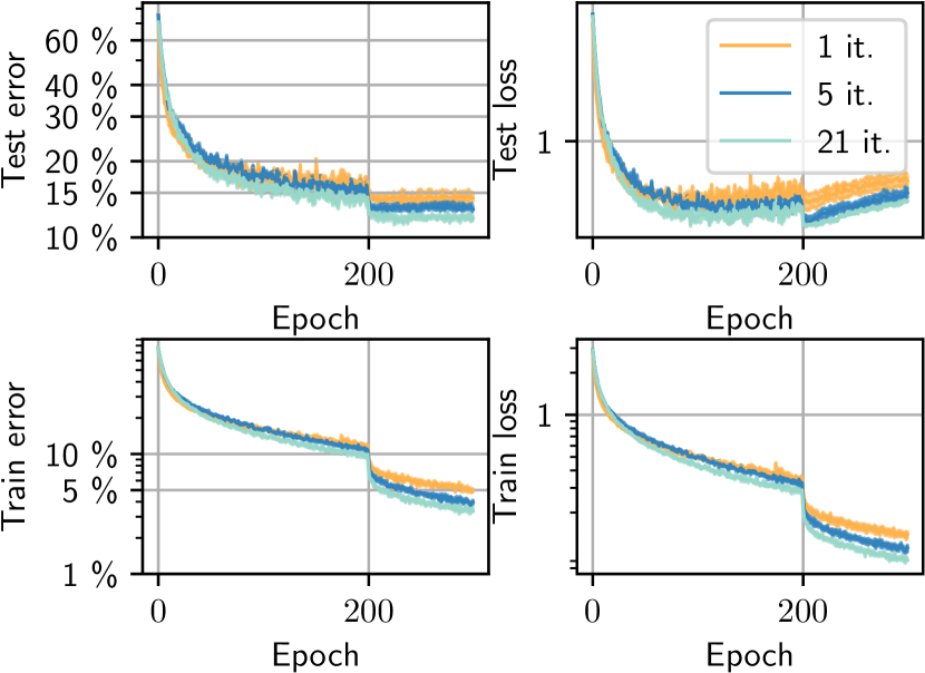
Figure 3: Classification error and loss on ModelNet 40 when training a Set Transformer and a Set Sinkformer with different number of iterations in Sinkhorn’s algorithm.

Figure 4: Learning curves when training a Transformer and a Sinkformer on the Sentiment Analysis task on the IMDb Dataset.

Moreover, we show in Figure 3 the learning curves corresponding to this experiment. Interestingly, the number of iterations within Sinkhorn’s algorithm increases the accuracy of the model. Note that we only consider an odd number of iterations since we always want to have row-wise stochastic attention matrices to be consistent with the properties of the SoftMax.

Point Cloud Transformers.

We also train Point Cloud Transformers (Guo et al.,, 2021) on ModelNet 40. This architecture achieves accuracy comparable to the state of the art on this dataset. We compare best and median test accuracy over $4$ runs. Results are reported in Table 1, where we see that while the best test-accuracy is narrowly achieved for the Transformer, the Sinkformer has a slightly better median accuracy.

Table 1: Test accuracy for ModelNet 40 over 4 runs for each model.

Model Best Median Mean Worst   Set Transformer $87.8\%$ $86.3\%$ $85.8\%$ $84.7\%$ Set Sinkformer $\mathbf{89.1}\%$ $\mathbf{88.4}\%$ $\mathbf{88.3}\%$ $\mathbf{88.1}\%$   Point Cloud Transformer $\mathbf{93.2}\%$ $92.5\%$ ${92.5}\%$ $92.3\%$ Point Cloud Sinkformer $93.1\%$ $\mathbf{92.8}\%$ $\mathbf{92.7}\%$ $\mathbf{92.5}\%$

6.2 Sentiment Analysis

We train a Transformer (composed of an attention-based encoder followed by a max-pooling layer) and a Sinkformer on the IMDb movie review dataset (Maas et al.,, 2011) for sentiment analysis. This text classification task consists of predicting whether a movie review is positive or negative. The learning curves are shown in Figure 4, with a gain in accuracy when using a Sinkformer. In this experiment, Sinkhorn’s algorithm converges perfectly in 3 iterations (the resulting attention matrices are doubly stochastic), which corresponds to the green curve. The Sinkformer only adds a small computational overhead, since the training time per epoch is $4$m $02$s for the Transformer against $4$m $22$s for the Sinkformer.

6.3 Neural Machine Translation

We train a Transformer and its Sinkformer counterpart using the fairseq (Ott et al.,, 2019) sequence modeling toolkit on the IWSLT’14 German to English dataset (Cettolo et al.,, 2014). The architecture used is composed of an encoder and a decoder, both of depth $6$. We plug Sinkhorn’s algorithm only into the encoder part. Indeed, in the decoder, we can only pay attention to previous positions in the output sequence. For this reason, we need a mask that prevents a straightforward application of Sinkhorn’s algorithm. We demonstrate that even when using the hyper-parameters used to optimally train the Transformer, we achieve a similar BLEU (Papineni et al.,, 2002) over $6$ runs. We first train a Transformer for $30$ epochs. On the evaluation set, we obtain a BLEU of $34.43$. We then consider a Sinkformer with the weights of the trained Transformer. Interestingly, even this un-adapted Sinkformer provides a median BLEU score of $33.81$. We then divide the learning rate by $10$ and retrain for $5$ additional epochs both the Transformer and the Sinkformer to obtain a median BLEU of respectively $34.68$ and $34.73$ (Table 2). Importantly, the runtime for one training epoch is almost the same for both models: $2$m $48$s (Transformer) against $2$m $52$s (Sinkformer).

Table 2: Median BLEU score over 6 runs on the IWSLT’14 German to English dataset. The score ^⋆ is when evaluating the Sinkformer with the weights of the trained Transformer.

Model Epoch 30 Epoch 35   Transformer $34.43$ $34.68$ Sinkformer $33.81^{\mathbf{\star}}$ $\mathbf{34.73}$

6.4 Vision Transformers

Vision Transformers (ViT) (Dosovitskiy et al.,, 2020) have recently emerged as a promising architecture for achieving state of the art performance on computer vision tasks (Zhai et al.,, 2021), using only attention based mechanisms by selecting patches of fixed size in images and feeding them into an attention mechanism.

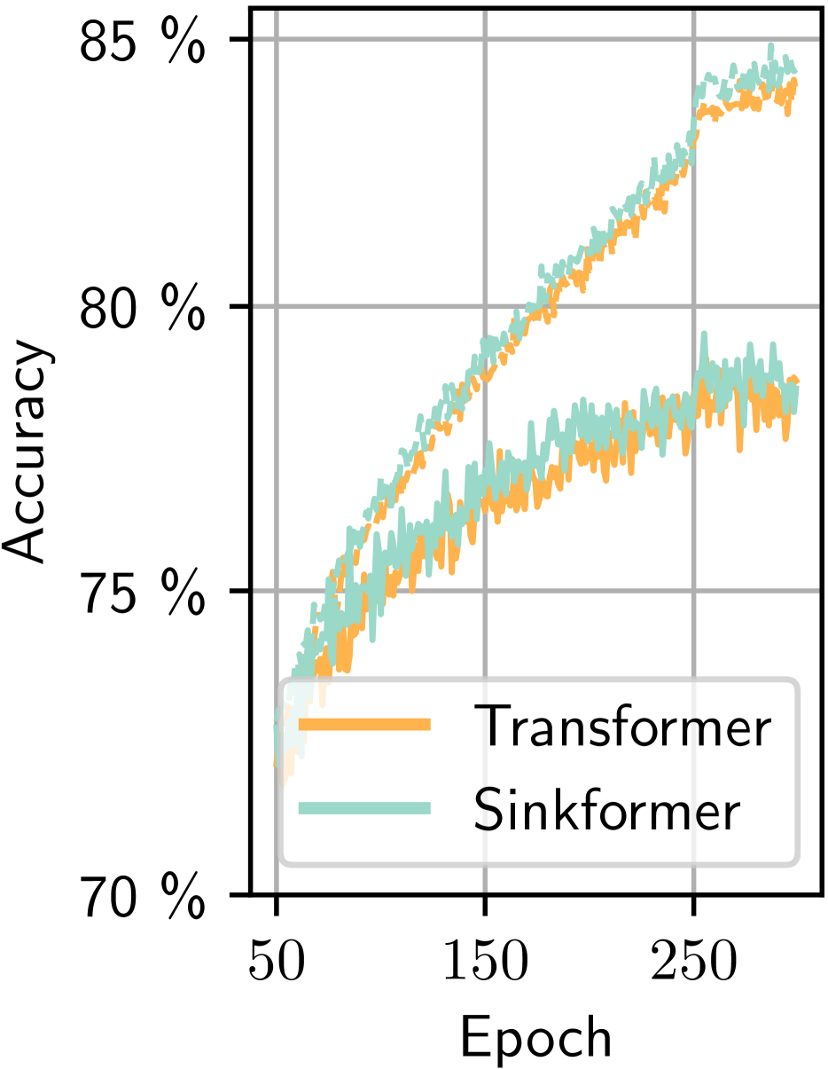
Figure 5: Train (dotted) and test (plain) accuracy as a function of the number of epochs when training a ViT and its Sinkformer counterpart on the cats and dogs classification task (median over 5 runs).

Cats and dogs classification.

We train a ViT and its Sinkformer counterpart on a binary cats and dogs image classification task. The evolution of the train and test accuracy is displayed in Figure 5. The median test accuracy is $79.0\%$ for the Transformer against $79.5\%$ for the Sinkformer, whereas the maximum test accuracy is $80.0\%$ for the Transformer against $80.5\%$ for the Sinkformer. We also use $3$ iterations in Sinkhorn’s algorithm which leads to a negligible computational overhead (training time per epoch of 3m 25s for the Sinkformer against 3m 20s for the Transformer).

Impact of the patch size on the final accuracy.

We consider a one-layer and one-head self-attention module on the MNIST dataset, with no additional layer. The purpose is to isolate the self-attention module and study how its accuracy is affected by the choice of the patch size. Results are displayed in Figure 6. We recall that a MNIST image is of size $28\times 28$. When taking only one patch of size $28$, both models are equivalent because the attention matrix is of size $1$. However, when the patch size gets smaller, the two models are different and the Sinkformer outperforms the Transformer.

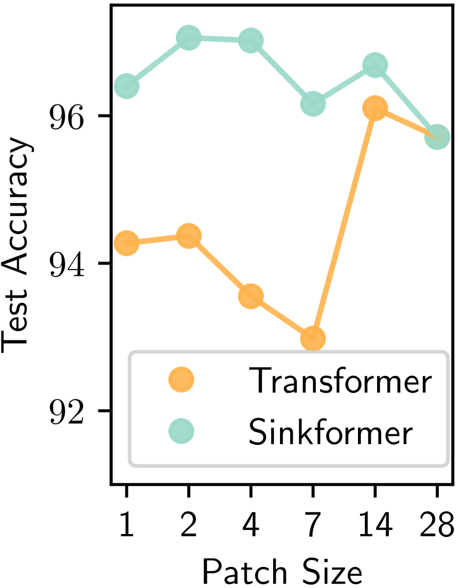
Figure 6: Final test accuracy when training a one layer and one head self attention module on the MNIST dataset, with no feedforward neural network, when varying the patch size (median over 5 runs).

Conclusion

In this paper, we presented the Sinkformer, a variant of the Transformer in which the SoftMax, which leads to row-wise stochastic attention, is replaced by Sinkhorn’s algorithm, which leads to doubly stochastic attention. This new model is motivated by the empirical finding that attention matrices in Transformers get closer and closer to doubly stochastic matrices during the training process. This modification is easily implemented in practice by simply replacing the SoftMax in the attention modules of existing Transformers without changing any parameter in the network. It also provides a new framework for theoretically studying attention-based mechanisms, such as the interpretation of Sinkformers as Wasserstein gradient flows in the infinitesimal step size regime or as diffusion operators in the mean-field limit. On the experimental side, Sinkformers lead to better accuracy in a variety of experiments: classification of 3D shapes, sentiment analysis, neural machine translation, and image classification.

Appendix

In Section A we give the proofs of all the Propositions and the Theorem. In Section B we present the implementation details of Sinkformers. Section C gives details for the experiments in the paper.

Appendix A Proofs

A.1 Invariance to the cost function - Proof of Proposition 1

Proof.

We use the variational formulation for Sinkhorn (Peyré et al.,, 2019):

$$\texttt{Sinkhorn}(C)=\operatorname{argmin}_{K\mathbb{1}_{n}=K^{\top}\mathbb{1}_{n}=\mathbb{1}_{n}}\mathrm{KL}(K|K^{0})$$

with

$$\mathrm{KL}(K|K^{0})=\sum_{i,j}K_{i,j}\log(\frac{K_{i,j}}{K^{0}_{i,j}}),$$

where $K^{0}_{i,j}=\exp(C_{i,j})$.

We let $\tilde{C}_{i,j}=C_{ij}+f_{i}+g_{j}$. We have for $K\in U\coloneqq\{K|K\mathbb{1}_{n}=K^{\top}\mathbb{1}_{n}=\mathbb{1}_{n}\}$ that $\mathrm{KL}(K|e^{\tilde{C}})=\sum_{i,j}K_{i,j}\log(\frac{K_{i,j}}{e^{C_{i,j}+f_{i}+g_{j}}})$. This gives

$$\mathrm{KL}(K|e^{\tilde{C}})=\sum_{i,j}K_{i,j}[\log(\frac{K_{i,j}}{e^{C_{i,j}}})-f_{i}-g_{j}]=\sum_{i,j}K_{i,j}[\log(\frac{K_{i,j}}{e^{C_{i,j}}})]-\sum_{i}f_{i}-\sum_{j}g_{j}$$

so that

$$\mathrm{KL}(K|e^{\tilde{C}})=\mathrm{KL}(K|e^{{C}})-\sum_{i}f_{i}-\sum_{j}g_{j}.$$

This shows that $\mathrm{KL}(K|e^{\tilde{C}})$ and $\mathrm{KL}(K|e^{{C}})$ have the same argmin on $U$ which implies that $\texttt{Sinkhorn}(C)=\texttt{Sinkhorn}(\tilde{C})$.

∎

A.2 PDEs associated with $\mathbf{k^{0},k^{1},k^{\infty}}$ - Proof of Proposition 2

Proof.

Recall that for $p\in\{0,1,\infty\}$, we have $T_{\mu}^{p}(x)=\int k^{p}(x,x^{\prime})W_{V}x^{\prime}d\mu(x^{\prime})$.

For $h\in\mathcal{C}(\mathbb{R}^{d}\times\mathbb{R}^{d})$ consider

$$\mathcal{H}(\mu)=\int h(x,y)d\mu(x)d\mu(y).$$

Then we have (Santambrogio,, 2017)

$$\frac{\delta\mathcal{H}}{\delta\mu}(\mu)=\int(h(x,.)+h(.,x))d\mu(x).$$

We can now derive the different gradient expressions for $T_{\mu}^{0}$, $T_{\mu}^{1}$ and $T_{\mu}^{\infty}$.

For $T_{\mu}^{0}$: under Assumption 1, we have that $f(x,x^{\prime})=e^{C(x,x^{\prime})}$ is symmetric. This gives

$$\frac{\delta\mathcal{F}}{\delta\mu}(\mu)=\int f(.,x^{\prime})d\mu(x^{\prime})$$

and by differentiation under the integral, under sufficient regularity assumptions on $\mu$, this gives

$$\nabla_{W}(\mathcal{F}^{0})(x)=\int\nabla_{x}f(x,x^{\prime})d\mu(x^{\prime})=\int f(x,x^{\prime})\nabla_{x}c(x,x^{\prime})d\mu(x^{\prime}).$$

Since $\nabla_{x}c(x,x^{\prime})=-W_{V}x^{\prime}$, we get

$$\nabla_{W}(\mathcal{F}^{0})(x)=-\int e^{c(x,x^{\prime})}W_{V}x^{\prime}d\mu(x^{\prime}).$$

For $\mu=\frac{1}{n}\sum_{i=1}^{n}\delta_{x_{i}}$ this is exactly

$$\nabla_{W}(\mathcal{F}^{0})(x)=-\sum^{n}_{j=1}K^{0}_{i,j}W_{V}x_{j}.$$

For $T_{\mu}^{1}$: we have

$$\nabla[\log(\int e^{c(.,x^{\prime})}d\mu(x^{\prime}))](x)=\int\frac{\nabla_{x}c(x,x^{\prime})e^{c(x,x^{\prime})}}{\int e^{c(x,y)}d\mu(y)}d\mu(x^{\prime})=-\int\frac{e^{c(x,x^{\prime})}W_{V}x^{\prime}}{\int e^{c(x,y)}d\mu(y)}d\mu(x^{\prime}).$$

For $T_{\mu}^{2}$: one has the dual formulation for $\mathcal{F}^{\infty}$ (Peyré et al.,, 2019):

$$2\mathcal{F}^{\infty}(\mu)=-\underset{f}{\max}\;\int_{\mathbb{R}^{d}}(f+f^{c})\text{d}\mu$$ (10)

where we denote the soft $c$ transform as

$$f^{c}(x^{\prime})\coloneqq-\log\left(\int e^{f(x)+c(x,x^{\prime})}\text{d}\mu(x)\right),$$ (11)

which actually depends on $\mu$ and $c$. One has for an optimal pair $f=f^{c}$ (Peyré et al.,, 2019). In addition, one has $k^{\infty}(x,x^{\prime})=e^{c(x,x^{\prime})+f(x)+f(x^{\prime})}$. The Wasserstein gradient of $\mathcal{F}^{\infty}$ is then

$$\nabla_{W}\mathcal{F}^{\infty}(\mu)=-\nabla f$$

where $f$ is an optimal solution of (10) (which is unique up to a constant). The gradient of $f$ can be obtained using (11) and the fact that $f=f^{c}$:

$$\nabla f(x)=-\int e^{f(x)+f(x^{\prime})+c(x,x^{\prime})}\nabla_{x}c(x,x^{\prime})d\mu(x^{\prime})=-\int k^{\infty}(x,x^{\prime})\nabla_{x}c(x,x^{\prime})d\mu(x^{\prime}).$$

This finally gives

$$\nabla_{W}\mathcal{F}^{\infty}(\mu):x\mapsto-\int k^{\infty}(x,x^{\prime})W_{v}x^{\prime}\text{d}\mu(x^{\prime}),$$ (12)

that is what we wanted to show. ∎

A.3 The SoftMax normalization does not correspond to a gradient flow - Proof of Proposition 3

Proof.

Suppose by contradiction that $T_{\mu}^{1}=-\nabla[\log(\int k^{0}(\cdot,x^{\prime})d\mu(x^{\prime}))]$ is a Wasserstein gradient. This implies that there exists a function $F$ such that, $\forall\mu\in\mathcal{M}(\mathbb{R}^{d})$ and $\forall x\in\mathbb{R}^{d}$,

$$\frac{\delta F}{\delta\mu}(\mu)(x)=\log(\int k^{0}(\cdot,x^{\prime})d\mu(x^{\prime})).$$

We therefore have

$$\frac{\delta^{2}F}{\delta\mu^{2}}(\mu)(x,x^{\prime})=\frac{k^{0}(x,x^{\prime})}{\int k^{0}(x,y)d\mu(y)},$$

$\forall x,x^{\prime}\in\mathbb{R}^{d}$. However, $\frac{\delta^{2}F}{\delta\mu^{2}}(\mu)$ is symmetric for all $\mu\in\mathcal{M}(\mathbb{R}^{d})$. The relationship $\frac{\delta^{2}F}{\delta\mu^{2}}(\mu)(x,x^{\prime})=\frac{\delta^{2}F}{\delta\mu^{2}}(\mu)(x^{\prime},x)$ then implies that for all $\mu$, $x$ and $x^{\prime}$ such that $k^{0}(x,x^{\prime})\neq 0$ we have

$$\int k^{0}(x,y)d\mu(y)=\int k^{0}(x^{\prime},y)d\mu(y).$$

Taking $\mu=\delta_{y}$ gives $k^{0}(x,y)=k^{0}(x^{\prime},y)$, which by symmetry implies that $k^{0}$ is a constant.

This is a contradiction since $k^{0}(x,x^{\prime})=\exp(x^{\top}W_{Q}^{\top}W_{K}x^{\prime})$. ∎

A.4 Sinkformer’s PDE - Proof of Theorem 1

Proof.

Since $W_{Q}^{\top}W_{K}$ is positive-definite we write it $W_{Q}^{\top}W_{K}=A^{2}$ where $A$ is positive-definite. Note that thanks to Proposition 1, if $\kappa_{\varepsilon}(x,x^{\prime})=\exp(-\frac{\|x-x^{\prime}\|^{2}}{2\varepsilon})$, one has under Assumption 1 that $\kappa^{\infty}_{\varepsilon}(Ax,Ax^{\prime})=k^{\infty}_{\varepsilon}(x,x^{\prime})$. For $x\in\mathbb{R}^{d}$, we have

$$\overline{T}^{\infty}_{\mu,\varepsilon}(A^{-1}x)=\frac{1}{\varepsilon}(\int\kappa^{\infty}_{\varepsilon}(x,Ax^{\prime})W_{V}x^{\prime}\rho(x^{\prime})dx^{\prime}-W_{V}A^{-1}x).$$

We perform the change of variable $y=Ax^{\prime}$. This gives

$$\overline{T}^{\infty}_{\mu,\varepsilon}(A^{-1}x)=\frac{1}{\varepsilon}(\int\kappa^{\infty}_{\varepsilon}(x,y)W_{V}A^{-1}y\rho(A^{-1}y)C_{A}dy-W_{V}A^{-1}x),$$

where $C_{A}$ depends only on $A$. We then apply Theorem 1 from Marshall and Coifman, (2019) with $f=W_{V}A^{-1}$, $q(x)=\rho(A^{-1}x)$ and $w=\frac{1}{C_{A}}$, to obtain that

$$\overline{T}^{\infty}_{\mu,\varepsilon}(A^{-1}\cdot)\to\frac{2\nabla f\nabla(q^{1/2})}{q^{1/2}}=W_{V}A^{-1}\frac{\nabla q}{q}$$

in $L^{2}$ norm. Since $q(x)=\rho(A^{-1}x)$ we have obtained that $\frac{\nabla q}{q}=A^{-1}\frac{\nabla\rho}{\rho}(A^{-1}\cdot)$ so that

$$\overline{T}^{\infty}_{\mu,\varepsilon}(A^{-1}x)\to W_{V}A^{-2}\frac{\nabla\rho}{\rho}(A^{-1}x)=W_{V}(W_{Q}^{\top}W_{K})^{-1}\frac{\nabla\rho}{\rho}(A^{-1}x).$$

In other words,

$$\overline{T}^{\infty}_{\mu,\varepsilon}\to W_{V}(W_{Q}^{\top}W_{K})^{-1}\frac{\nabla\rho}{\rho},$$

which is exactly what we wanted to show. Note that when $W_{V}=-W_{Q}^{\top}W_{K}$ this gives the expected result. The general form for the PDE is then

$$\partial_{t}\rho=\mathrm{div}(-W_{V}(W_{Q}^{\top}W_{K})^{-1}\frac{\nabla\rho}{\rho}\times\rho)$$

which gives

$$\partial_{t}\rho=\Delta\rho$$

if $W_{V}=-W_{Q}^{\top}W_{K}$. ∎

A.5 Transformer’s PDE - Proof of Proposition 4

Proof.

Let $x\in\mathbb{R}^{d}$ and consider

$$g_{\varepsilon}(x)=\varepsilon T^{1}_{\mu,\varepsilon}(W^{-1}_{Q}x)=\frac{\int e^{-\frac{\|x-W_{K}x^{\prime}\|^{2}}{2\varepsilon}}W_{V}x^{\prime}\rho(x^{\prime})dx^{\prime}}{\int e^{-\frac{\|x-W_{K}x^{\prime}\|^{2}}{2\varepsilon}}\rho(x^{\prime})dx^{\prime}}.$$

We perform the change of variable $y=W_{K}x^{\prime}$. This gives:

$$g_{\varepsilon}(x)=\frac{\int e^{-\frac{\|x-y\|^{2}}{2\varepsilon}}W_{V}W^{-1}_{K}y\rho(W^{-1}_{K}y)dy}{\int e^{-\frac{\|x-y^{\prime}\|^{2}}{2\varepsilon}}\rho(W^{-1}_{K}y)dy}.$$

Using the Laplace expansion result from Singer, (2006), we obtain that

$$g_{\varepsilon}(x)=W_{V}W^{-1}_{K}\frac{x\rho(W^{-1}_{K}x)+\frac{\varepsilon}{2}\Delta(x\rho(W^{-1}_{K}x))+o(\varepsilon)}{\rho(W^{-1}_{K}x)+\frac{\varepsilon}{2}\Delta(\rho(W^{-1}_{K}x))+o(\varepsilon).}$$

By doing a Taylor expansion for the denominator, we find

$$g_{\varepsilon}(x)=W_{V}W^{-1}_{K}(x+\frac{\varepsilon}{2}\frac{\Delta(x\rho(W^{-1}_{K}x)}{\rho(W^{-1}_{K}x)}+o(\varepsilon))(1-\frac{\varepsilon}{2}\frac{\Delta(\rho(W^{-1}_{K}x))}{\rho(W^{-1}_{K}x)}+o(\varepsilon))$$

and

$$g_{\varepsilon}(x)=W_{V}W^{-1}_{K}(x+\varepsilon\frac{\nabla(\rho(W^{-1}_{K}x))}{\rho(W^{-1}_{K}x)}+o(\varepsilon).)$$

Since $\overline{T}^{1}_{\mu,\varepsilon}={T}^{1}_{\mu,\varepsilon}+\frac{1}{\varepsilon}W_{Q}^{\top}W_{Q}=\frac{1}{\varepsilon}(g_{\varepsilon}(W_{Q}x)+W_{Q}^{\top}W_{Q}x)$ and because $W_{V}W^{-1}_{K}=-{W_{Q}}^{\top}W_{K}W^{-1}_{K}=-W^{\top}_{Q}$ we have

$$\overline{T}^{1}_{\mu,\varepsilon}=-W^{\top}_{Q}W^{-1}_{K}\frac{\nabla\rho(W^{-1}_{K}W_{Q}x))}{\rho(W^{-1}_{K}W_{Q}x)}+o(1)$$

which is exactly the expected result. ∎

Appendix B Implementation details

We implement Sinkhorn’s algorithm in log domain for stability. Given a matrix $K^{0}\in\mathbb{R}^{n\times n}$ such that $K^{0}_{i,j}=e^{C_{i,j}}$ for some $C\in\mathbb{R}^{n\times n}$, Sinkhorn’s algorithm (3) approaches $(f,g)\in\mathbb{R}^{n}\times\mathbb{R}^{n}$ such that $K^{\infty}=\mathrm{diag}(e^{f^{\infty}})K^{0}\mathrm{diag}(e^{g^{\infty}})$ by iterating in $\log$ domain, starting from $g^{0}=\mathbb{0}_{n}$,

$$\begin{split}f^{l+1}&=\log(\mathbb{1}_{n}/n)-\log({Ke^{g^{l}}})\quad\text{if $l$ is even}\\ g^{l+1}&=\log(\mathbb{1}_{n}/n)-\log({K^{\top}e^{f^{l}}})\quad\text{if $l$ is odd}.\end{split}$$ (13)

This allows for fast and accurate computations, where $\log({Ke^{g^{l}}})$ and $\log({K^{\top}e^{f^{l}}})$ are computed using log-sum-exp.

Appendix C Experimental details

C.1 ModelNet 40 classification

Set Transformers.

For our experiments on ModelNet using Set Transformers, we first prepossess the ModelNet 40 dataset. We then uniformly sample $5000$ points from each element in the dataset. Our architecture is composed of two ISAB layers in the encoder and a decoder composed of a SAB and a Pooling by Multihead Attention (PMA) module. For the training, we use a batch-size of $64$ and we use Adam (Kingma and Ba,, 2014). The training is done over $300$ epochs. The initial learning rate is $10^{-3}$ and is decayed by a factor $10$ after $200$ epochs.

Point Cloud Transformers.

For our experiments on ModelNet using Point Clouds Transformers, we uniformly sample $1024$ points from each element in the dataset. For the training, we use a batch-size of $32$ and we use SGD (Ruder,, 2016). The training is done over $300$ epochs. The initial learning rate is $10^{-4}$ and is decayed by a factor $10$ after $250$ epochs.

C.2 Sentiment Analysis

We use the code available at the repository nlp-turorial, where a pretrained Transformer is fine-tuned on the IMDb dataset. In our experiment, we reset the parameters of the pretrained Transformer and train it from scratch on the IMDb dataset. We use an architecture of depth $6$, with $8$ heads. For the training, we use a batch-size of $32$ and we use Adam. The training is done over $15$ epochs. The initial learning rate is $10^{-4}$ and is decayed by a factor $10$ after $12$ epochs.

C.3 Neural Machine Translation

We use the Transformer from fairseq and the command for training it on the IWSLT’14 dataset. When fine-tuning a Sinkformer, we simply divide the original learning rate by $10$.

C.4 Vision Transformers

Cats and dogs classification.

This experiment is done on the cats and dogs dataset. For this experiment, we use a batch-size of $64$ and Adam. We use an architecture of depth $6$, with $8$ heads, and select a patch-size of $16$. The training is done over $300$ epochs. The initial learning rate is $5\times 10^{-5}$ and divided by $10$ after $250$ epochs.

Impact of the patch size on the final accuracy.

For this experiment, we use a batch-size of $100$ and Adam. We use an architecture of depth $1$, with $1$ heads, without non-linearity, and select different values for the patch-size. The training is done over $45$ epochs. The initial learning rate is $1\times 10^{-3}$ (resp. $2\times 10^{-3}$) for the Transformer (resp. Sinkformer) and divided by $10$ after $35$ epochs and again by $10$ after $41$ epochs.

References

- Agrawal et al., (2019) Agrawal, A., Amos, B., Barratt, S., Boyd, S., Diamond, S., and Kolter, Z. (2019). Differentiable convex optimization layers. arXiv preprint arXiv:1910.12430.
- Bahdanau et al., (2014) Bahdanau, D., Cho, K., and Bengio, Y. (2014). Neural machine translation by jointly learning to align and translate. arXiv preprint arXiv:1409.0473.
- Bai et al., (2019) Bai, S., Kolter, J. Z., and Koltun, V. (2019). Deep equilibrium models. Advances in Neural Information Processing Systems, 32:690–701.
- Behrmann et al., (2019) Behrmann, J., Grathwohl, W., Chen, R. T., Duvenaud, D., and Jacobsen, J.-H. (2019). Invertible residual networks. In International Conference on Machine Learning, pages 573–582. PMLR.
- Blondel et al., (2021) Blondel, M., Berthet, Q., Cuturi, M., Frostig, R., Hoyer, S., Llinares-López, F., Pedregosa, F., and Vert, J.-P. (2021). Efficient and modular implicit differentiation. arXiv preprint arXiv:2105.15183.
- Brown et al., (2020) Brown, T. B., Mann, B., Ryder, N., Subbiah, M., Kaplan, J., Dhariwal, P., Neelakantan, A., Shyam, P., Sastry, G., Askell, A., et al. (2020). Language models are few-shot learners. arXiv preprint arXiv:2005.14165.
- Cettolo et al., (2014) Cettolo, M., Niehues, J., Stüker, S., Bentivogli, L., and Federico, M. (2014). Report on the 11th iwslt evaluation campaign, iwslt 2014. In Proceedings of the International Workshop on Spoken Language Translation, Hanoi, Vietnam, volume 57.
- Charlier et al., (2021) Charlier, B., Feydy, J., Glaunès, J., Collin, F.-D., and Durif, G. (2021). Kernel operations on the gpu, with autodiff, without memory overflows. Journal of Machine Learning Research, 22(74):1–6.
- Chen et al., (2018) Chen, T. Q., Rubanova, Y., Bettencourt, J., and Duvenaud, D. K. (2018). Neural ordinary differential equations. In Advances in neural information processing systems, pages 6571–6583.
- Cuturi, (2013) Cuturi, M. (2013). Sinkhorn distances: Lightspeed computation of optimal transport. Advances in neural information processing systems, 26:2292–2300.
- Cuturi et al., (2020) Cuturi, M., Teboul, O., Niles-Weed, J., and Vert, J.-P. (2020). Supervised quantile normalization for low rank matrix factorization. In International Conference on Machine Learning, pages 2269–2279. PMLR.
- De Bie et al., (2019) De Bie, G., Peyré, G., and Cuturi, M. (2019). Stochastic deep networks. In International Conference on Machine Learning, pages 1556–1565. PMLR.
- Dong et al., (2021) Dong, Y., Cordonnier, J.-B., and Loukas, A. (2021). Attention is not all you need: Pure attention loses rank doubly exponentially with depth. arXiv preprint arXiv:2103.03404.
- Dosovitskiy et al., (2020) Dosovitskiy, A., Beyer, L., Kolesnikov, A., Weissenborn, D., Zhai, X., Unterthiner, T., Dehghani, M., Minderer, M., Heigold, G., Gelly, S., et al. (2020). An image is worth 16x16 words: Transformers for image recognition at scale. arXiv preprint arXiv:2010.11929.
- Gould et al., (2016) Gould, S., Fernando, B., Cherian, A., Anderson, P., Cruz, R. S., and Guo, E. (2016). On differentiating parameterized argmin and argmax problems with application to bi-level optimization. arXiv preprint arXiv:1607.05447.
- Gould et al., (2019) Gould, S., Hartley, R., and Campbell, D. (2019). Deep declarative networks: A new hope. arXiv preprint arXiv:1909.04866.
- Griewank and Walther, (2008) Griewank, A. and Walther, A. (2008). Evaluating derivatives: principles and techniques of algorithmic differentiation. SIAM.
- Guo et al., (2021) Guo, M.-H., Cai, J.-X., Liu, Z.-N., Mu, T.-J., Martin, R. R., and Hu, S.-M. (2021). Pct: Point cloud transformer. Computational Visual Media, 7(2):187–199.
- He et al., (2016) He, K., Zhang, X., Ren, S., and Sun, J. (2016). Deep residual learning for image recognition. In Proceedings of the IEEE conference on computer vision and pattern recognition, pages 770–778.
- Hein et al., (2007) Hein, M., Audibert, J.-Y., and Luxburg, U. v. (2007). Graph laplacians and their convergence on random neighborhood graphs. Journal of Machine Learning Research, 8(6).
- Jordan et al., (1998) Jordan, R., Kinderlehrer, D., and Otto, F. (1998). The variational formulation of the fokker–planck equation. SIAM journal on mathematical analysis, 29(1):1–17.
- Kim et al., (2021) Kim, H., Papamakarios, G., and Mnih, A. (2021). The lipschitz constant of self-attention. In International Conference on Machine Learning, pages 5562–5571. PMLR.
- Kingma and Ba, (2014) Kingma, D. P. and Ba, J. (2014). Adam: A method for stochastic optimization. arXiv preprint arXiv:1412.6980.
- Krantz and Parks, (2012) Krantz, S. G. and Parks, H. R. (2012). The implicit function theorem: history, theory, and applications. Springer Science & Business Media.
- Lee et al., (2019) Lee, J., Lee, Y., Kim, J., Kosiorek, A., Choi, S., and Teh, Y. W. (2019). Set transformer: A framework for attention-based permutation-invariant neural networks. In International Conference on Machine Learning, pages 3744–3753. PMLR.
- Lu et al., (2018) Lu, Y., Zhong, A., Li, Q., and Dong, B. (2018). Beyond finite layer neural networks: Bridging deep architectures and numerical differential equations. In International Conference on Machine Learning, pages 3276–3285. PMLR.
- Luise et al., (2018) Luise, G., Rudi, A., Pontil, M., and Ciliberto, C. (2018). Differential properties of sinkhorn approximation for learning with wasserstein distance. arXiv preprint arXiv:1805.11897.
- Maas et al., (2011) Maas, A. L., Daly, R. E., Pham, P. T., Huang, D., Ng, A. Y., and Potts, C. (2011). Learning word vectors for sentiment analysis. In Proceedings of the 49th Annual Meeting of the Association for Computational Linguistics: Human Language Technologies, pages 142–150, Portland, Oregon, USA. Association for Computational Linguistics.
- Marshall and Coifman, (2019) Marshall, N. F. and Coifman, R. R. (2019). Manifold learning with bi-stochastic kernels. IMA Journal of Applied Mathematics, 84(3):455–482.
- Mialon et al., (2021) Mialon, G., Chen, D., d’Aspremont, A., and Mairal, J. (2021). A trainable optimal transport embedding for feature aggregation and its relationship to attention. In ICLR 2021-The Ninth International Conference on Learning Representations.
- Milanfar, (2013) Milanfar, P. (2013). Symmetrizing smoothing filters. SIAM Journal on Imaging Sciences, 6(1):263–284.
- Niculae et al., (2018) Niculae, V., Martins, A., Blondel, M., and Cardie, C. (2018). Sparsemap: Differentiable sparse structured inference. In International Conference on Machine Learning, pages 3799–3808. PMLR.
- Ott et al., (2019) Ott, M., Edunov, S., Baevski, A., Fan, A., Gross, S., Ng, N., Grangier, D., and Auli, M. (2019). fairseq: A fast, extensible toolkit for sequence modeling. In Proceedings of NAACL-HLT 2019: Demonstrations.
- Papineni et al., (2002) Papineni, K., Roukos, S., Ward, T., and Zhu, W.-J. (2002). Bleu: a method for automatic evaluation of machine translation. In Proceedings of the 40th annual meeting of the Association for Computational Linguistics, pages 311–318.
- Paszke et al., (2017) Paszke, A., Gross, S., Chintala, S., Chanan, G., Yang, E., DeVito, Z., Lin, Z., Desmaison, A., Antiga, L., and Lerer, A. (2017). Automatic differentiation in pytorch.
- Peng et al., (2017) Peng, C., Zhang, X., Yu, G., Luo, G., and Sun, J. (2017). Large kernel matters–improve semantic segmentation by global convolutional network. In Proceedings of the IEEE conference on computer vision and pattern recognition, pages 4353–4361.
- Peyré et al., (2019) Peyré, G., Cuturi, M., et al. (2019). Computational optimal transport: With applications to data science. Foundations and Trends® in Machine Learning, 11(5-6):355–607.
- Radford et al., (2019) Radford, A., Wu, J., Child, R., Luan, D., Amodei, D., Sutskever, I., et al. (2019). Language models are unsupervised multitask learners. OpenAI blog, 1(8):9.
- Renardy and Rogers, (2006) Renardy, M. and Rogers, R. C. (2006). An introduction to partial differential equations, volume 13. Springer Science & Business Media.
- Ruder, (2016) Ruder, S. (2016). An overview of gradient descent optimization algorithms. arXiv preprint arXiv:1609.04747.
- Ruthotto and Haber, (2019) Ruthotto, L. and Haber, E. (2019). Deep neural networks motivated by partial differential equations. Journal of Mathematical Imaging and Vision, pages 1–13.
- Sander et al., (2021) Sander, M. E., Ablin, P., Blondel, M., and Peyré, G. (2021). Momentum residual neural networks. In Proceedings of the 38th International Conference on Machine Learning, volume 139 of Proceedings of Machine Learning Research, pages 9276–9287. PMLR.
- Santambrogio, (2017) Santambrogio, F. (2017). Euclidean, metric, and Wasserstein gradient flows: an overview. Bulletin of Mathematical Sciences, 7(1):87–154.
- Singer, (2006) Singer, A. (2006). From graph to manifold laplacian: The convergence rate. Applied and Computational Harmonic Analysis, 21(1):128–134.
- Sinkhorn, (1964) Sinkhorn, R. (1964). A relationship between arbitrary positive matrices and doubly stochastic matrices. The annals of mathematical statistics, 35(2):876–879.
- Song et al., (2018) Song, M., Montanari, A., and Nguyen, P. (2018). A mean field view of the landscape of two-layers neural networks. Proceedings of the National Academy of Sciences, 115:E7665–E7671.
- Sun et al., (2018) Sun, Q., Tao, Y., and Du, Q. (2018). Stochastic training of residual networks: a differential equation viewpoint. arXiv preprint arXiv:1812.00174.
- Tay et al., (2020) Tay, Y., Bahri, D., Yang, L., Metzler, D., and Juan, D.-C. (2020). Sparse sinkhorn attention. In International Conference on Machine Learning, pages 9438–9447. PMLR.
- Teh et al., (2019) Teh, Y., Doucet, A., and Dupont, E. (2019). Augmented neural odes. Advances in Neural Information Processing Systems 32 (NIPS 2019), 32(2019).
- Tierney et al., (1989) Tierney, L., Kass, R. E., and Kadane, J. B. (1989). Fully exponential laplace approximations to expectations and variances of nonpositive functions. Journal of the american statistical association, 84(407):710–716.
- Ting et al., (2011) Ting, D., Huang, L., and Jordan, M. (2011). An analysis of the convergence of graph laplacians. arXiv preprint arXiv:1101.5435.
- Vaswani et al., (2017) Vaswani, A., Shazeer, N., Parmar, N., Uszkoreit, J., Jones, L., Gomez, A. N., Kaiser, Ł., and Polosukhin, I. (2017). Attention is all you need. In Advances in neural information processing systems, pages 5998–6008.
- Vuckovic et al., (2021) Vuckovic, J., Baratin, A., and Combes, R. T. d. (2021). On the regularity of attention. arXiv preprint arXiv:2102.05628.
- Wang et al., (2018) Wang, L., Ye, J., Zhao, Y., Wu, W., Li, A., Song, S. L., Xu, Z., and Kraska, T. (2018). Superneurons: Dynamic gpu memory management for training deep neural networks. In Proceedings of the 23rd ACM SIGPLAN Symposium on Principles and Practice of Parallel Programming, pages 41–53.
- Weinan, (2017) Weinan, E. (2017). A proposal on machine learning via dynamical systems. Communications in Mathematics and Statistics, 5(1):1–11.
- Weinan et al., (2019) Weinan, E., Han, J., and Li, Q. (2019). A mean-field optimal control formulation of deep learning. Research in the Mathematical Sciences, 6(1):10.
- Wolf et al., (2019) Wolf, T., Debut, L., Sanh, V., Chaumond, J., Delangue, C., Moi, A., Cistac, P., Rault, T., Louf, R., Funtowicz, M., et al. (2019). Huggingface’s transformers: State-of-the-art natural language processing. arXiv preprint arXiv:1910.03771.
- Wormell and Reich, (2021) Wormell, C. L. and Reich, S. (2021). Spectral convergence of diffusion maps: Improved error bounds and an alternative normalization. SIAM Journal on Numerical Analysis, 59(3):1687–1734.
- Wu et al., (2015) Wu, Z., Song, S., Khosla, A., Yu, F., Zhang, L., Tang, X., and Xiao, J. (2015). 3d shapenets: A deep representation for volumetric shapes. In Proceedings of the IEEE conference on computer vision and pattern recognition, pages 1912–1920.
- Yun et al., (2019) Yun, C., Bhojanapalli, S., Rawat, A. S., Reddi, S. J., and Kumar, S. (2019). Are transformers universal approximators of sequence-to-sequence functions? arXiv preprint arXiv:1912.10077.
- Zhai et al., (2021) Zhai, X., Kolesnikov, A., Houlsby, N., and Beyer, L. (2021). Scaling vision transformers. arXiv preprint arXiv:2106.04560.
- Zhao et al., (2020) Zhao, H., Jiang, L., Jia, J., Torr, P., and Koltun, V. (2020). Point transformer. arXiv preprint arXiv:2012.09164.
- Zhu et al., (2017) Zhu, J.-Y., Park, T., Isola, P., and Efros, A. A. (2017). Unpaired image-to-image translation using cycle-consistent adversarial networks. In Proceedings of the IEEE international conference on computer vision, pages 2223–2232.
- Zweig and Bruna, (2021) Zweig, A. and Bruna, J. (2021). A functional perspective on learning symmetric functions with neural networks. In International Conference on Machine Learning, pages 13023–13032. PMLR.