QCD-based estimate of direct $CP$ asymmetry
in charm decays

Abstract

I discuss the calculation of the direct CP-asymmetry in $D\to\pi^{+}\pi^{-}$ and $D\to K^{+}K^{-}$ decays with the method of QCD light-cone sum rules. The main result is the upper limit for the difference of the two asymmetries $\left|\Delta a_{CP}^{dir}\right|<0.020\pm 0.003\%$ which is significantly smaller than the recent measurement of this quantity by the LHCb collaboration.

1 Introduction

The $CP$ asymmetry measured by LHCb collaboration [1] in the single Cabibbo suppressed decays $D\to\pi^{+}\pi^{-}$ and $D\to K^{+}K^{-}$ remains a challenge for the theory. A quantitative estimate of this asymmetry in the Standard Model (SM) involves hadronic matrix elements with two energetic mesons in the final state that are not accessible yet with the lattice QCD methods. Hence, even approximate estimates of the $CP$ asymmetry obtained using other QCD based methods are useful, in order to trace or at least constrain the possible beyond SM contributions (see e.g., [2]).

Here I will discuss a calculation [3] of the direct CP-asymmetry in $D\to\pi^{+}\pi^{-}$ and $D\to K^{+}K^{-}$ decays with the method of light-cone sum rules (LCSRs). As shown in section 2, for each of these decays it is sufficient to calculate the CKM suppressed part of the decay amplitude with the penguin topology. In section 3, I briefly explain the idea of the LCSR method in a simplified version with a two-point correlation function. Section 4 presents the actual LCSR for the penguin hadronic matrix element, obtained with a more involved procedure using the three-point correlation function. We transfer to charm decays the method of LCSRs for $B\to\pi\pi$ decays initiated in [4] and developed further in [5, 6]. Our numerical result for the upper bound of the difference of direct CP asymmetries $\Delta a_{CP}$ is compared with the LHCb measurement [1]. In conclusion, I discuss the uncertainties and perspectives of our method.

2 Relating direct CP-asymmetry to the penguin amplitude

At the quark level, the single Cabibbo suppressed decays $D\to\pi\pi$ and $D\to K\bar{K}$ are generated by the effective Hamiltonian

$$H_{eff}=\frac{G_{F}}{\sqrt{2}}\Big{\{}\lambda_{d}\big{(}c_{1}~{}O_{1}^{d}+c_{2}~{}O_{2}^{d}\big{)}+\lambda_{s}\big{(}c_{1}~{}O_{1}^{s}+c_{2}~{}O_{2}^{s}\big{)}-\lambda_{b}\!\!\!\!\sum\limits_{i=3,...,6,8g}c_{i}O_{i}\Big{\}}\,,$$ (1)

where the operators $O_{1}^{d}=\left(\bar{u}\Gamma_{\mu}d\right)\left(\bar{d}\Gamma^{\mu}c\right)$ ,  $O_{2}^{d}=\left(\bar{d}\Gamma_{\mu}d\right)\left(\bar{u}\Gamma^{\mu}c\right)$ are multiplied with the Wilson coefficients $c_{1,2}$ and in $O^{s}_{1}\,,~{}O^{s}_{2}$ the $d$ quark is replaced by $s$ quark. Here, $\lambda_{q}=V_{uq}V_{cq}^{*},~{}~{}(q=d,s,b)$ are the relevant combinations of the CKM parameters.

Separating the contributions of the ${\cal O}^{d}_{1,2}$ and ${\cal O}^{s}_{1,2}$ operators and introducing a compact notation

$${\cal O}^{q}\equiv\sum_{i=1,2}c_{i}O_{i}^{q}\,~{}~{}(q=d,s),$$

we have for the decay amplitudes (in the units of $G_{F}/\sqrt{2}$):

$$A(D^{0}\to\pi^{+}\pi^{-})=\lambda_{d}\langle\pi^{+}\pi^{-}|{\cal O}^{d}|D^{0}\rangle+\lambda_{s}\langle\pi^{+}\pi^{-}|{\cal O}^{s}|D^{0}\rangle\,,$$ (2)

$$A(D^{0}\to K^{+}K^{-})=\lambda_{s}\langle K^{+}K^{-}|{\cal O}^{s}|D^{0}\rangle+\lambda_{d}\langle K^{+}K^{-}|{\cal O}^{d}|D^{0}\rangle\,.$$ (3)

Note that both decay amplitudes contain hadronic matrix elements with "penguin topology”

$$\langle\pi^{+}\pi^{-}|{\cal O}^{s}|D^{0}\rangle\equiv{\cal P}_{\pi\pi}^{s}\,,~{}~{}~{}~{}\langle K^{+}K^{-}|{\cal O}^{d}|D^{0}\rangle\equiv{\cal P}_{KK}^{d}\,,$$ (4)

in which the quark operator contains a $\bar{q}q$ pair with a flavour $q=s$ or $d$ absent in the valence content of the initial and final hadronic states. This definition is somewhat more general than specifying certain quark-flow diagrams (quark topologies).

Furthermore, using the CKM unitarity in SM: $\sum_{q=d,s,b}\lambda_{q}=0\,,$ we find it convenient to eliminate $\lambda_{d}=-(\lambda_{s}+\lambda_{b})\,,$ so that the amplitudes (2) and (3) are written in the form

$$A(D^{0}\to\pi^{+}\pi^{-}) = -\lambda_{s}{\cal A}_{\pi\pi}\Big{\{}1+\frac{\lambda_{b}}{\lambda_{s}}\Big{(}1+r_{\pi}\exp(i\delta_{\pi})\Big{)}\Big{\}}\,,$$ (5)

$$A(D^{0}\to K^{+}K^{-}) = \lambda_{s}{\cal A}_{KK}\Big{\{}1-\frac{\lambda_{b}}{\lambda_{s}}r_{K}\exp(i\delta_{K})\Big{\}}\,,$$ (6)

with the notation

$${\cal A}_{\pi\pi}=\langle\pi^{+}\pi^{-}|{\cal O}^{d}|D^{0}\rangle-\langle\pi^{+}\pi^{-}|{\cal O}^{s}|D^{0}\rangle\,,~{}~{}{\cal A}_{KK}=\langle K^{+}K^{-}|{\cal O}^{s}|D^{0}\rangle-\langle K^{+}K^{-}|{\cal O}^{d}|D^{0}\rangle\,,$$ (7)

and

$$r_{\pi}=\left|\frac{{\cal P}_{\pi\pi}^{s}}{{\cal A}_{\pi\pi}}\right|\,,~{}~{}r_{K}=\left|\frac{{\cal P}_{KK}^{d}}{{\cal A}_{KK}}\right|\,,~{}\delta_{\pi(K)}=arg[{\cal P}_{\pi\pi(KK)}^{s(d)}]-arg[{\cal A}_{\pi\pi(KK)}]\,.$$ (8)

In (5) and (6) only the contributions proportional to $\lambda_{b}$, with $\mbox{Im}(\lambda_{b})\neq 0$, contain the CP-violating phase. The conditions for a nonvanishing direct $CP$ asymmetry are clearly fulfilled: both decay amplitudes consist of two parts with different weak and strong phases. Defining this asymmetry as

$$a_{CP}^{dir}(f)=\frac{\Gamma(D^{0}\to f)-\Gamma(\bar{D}^{0}\to\bar{f})}{\Gamma(D^{0}\to f)+\Gamma(\bar{D}^{0}\to\bar{f})}\,,~{}~{}~{}f=\pi^{+}\pi^{-},\,K^{+}K^{-}\,,$$ (9)

and using (5) and (6), we obtain:

$$a_{CP}^{dir}(K^{+}K^{-})=\frac{-2r_{b}r_{K}\sin\delta_{K}\sin\gamma}{1-2r_{b}r_{K}\cos\gamma\cos\delta_{K}+r_{b}^{2}r_{K}^{2}}\,,$$ (10)

$$a_{CP}^{dir}(\pi^{+}\pi^{-})=\frac{2r_{b}r_{\pi}\sin\delta_{\pi}\sin\gamma}{1+2r_{b}\cos\gamma(1+r_{\pi}\cos\delta_{\pi})+r_{b}^{2}(1+2r_{\pi}\cos\delta_{\pi}+r_{\pi}^{2})}\,,$$ (11)

were the ratio of the CKM matrix elements is parameterized as

$$\frac{\lambda_{b}}{\lambda_{s}}\equiv r_{b}e^{-i\gamma},~{}~{}r_{b}=\Bigg{|}\frac{V_{ub}V_{cb}^{*}}{V_{us}V_{cs}^{*}}\Bigg{|}\,.$$ (12)

Furthermore, it is important that $|\lambda_{b}|\ll|\lambda_{s,d}|$, hence both equations (10) and (11) can be expanded in $r_{b}$ retaining the first power. As well known, a more "clean" observable (after the time integration) than the individual $CP$ asymmetries (10) and (11) is their difference:

$$\Delta a_{CP}^{dir} = a_{CP}^{dir}(K^{+}K^{-})-a_{CP}^{dir}(\pi^{+}\pi^{-})$$ (13)

$$= -2r_{b}\sin\gamma(r_{K}\sin\delta_{K}+r_{\pi}\sin\delta_{\pi})+O(r_{b}^{2})\,,$$

where the hadronic input is reduced to the two ratios and two phase differences defined in (8). At first sight, it seems that we have unnecessarily complicated our task defining the combinations ${\cal A}_{\pi\pi}$ and ${\cal A}_{KK}$ of the hadronic matrix elements. In fact, the key point is that, due to the smallness of $|\lambda_{b}|$, from (5) and (6) we have, to a good approximation,

$$-\lambda_{s}{\cal A}_{\pi\pi}\simeq A(D^{0}\to\pi^{+}\pi^{-})\,,~{}~{}~{}\lambda_{s}{\cal A}_{KK}\simeq A(D^{0}\to K^{+}K^{-})\,.$$

Thus, the denominators of the ratios $r_{K}$ and $r_{\pi}$ are obtained from the experimentally measured widths of these two decays. The estimate of direct $CP$ asymmetries (10) and (11) in SM is then reduced to the calculation of the two hadronic matrix elements ${\cal P}_{\pi\pi}^{s}$ and ${\cal P}_{KK}^{d}$ defined in (4).

3 Outline of the LCSR method

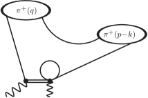
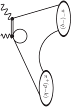
Figure 1: The diagram illustrating OPE for the correlation function (14) for the spacelike (left) and timelike (right) invariant variable $P^{2}=(p-k-q)^{2}$. Shown are the $s$-quark loop and the virtual $c$ quark (double line). The wavy lines denote external momenta $(p-q)$ and $k$ flowing, respectively, to the interpolating current and from the weak operator vertex.

These hadronic matrix elements were calculated in [3], employing the LCSR method formulated and applied to the $B\to\pi\pi$ decay in [4, 5, 6]. Let me first outline a somewhat simplified version of that method, in which the starting object is a two-point correlation function. Considering e.g., the $D\to\pi\pi$ decay, we introduce:

$$\Pi_{\pi\pi}((p-q)^{2},P^{2})=i\int\!d^{4}x\,e^{-i(p-q)x}\!\langle\pi^{+}(p-k)|T\{{\cal O}^{s}(0)j_{5}^{(D)}(x)\}|\pi^{+}(q)\rangle\,,$$ (14)

where $j_{5}^{(D)}=m_{c}\bar{c}i\gamma_{5}u$ is the $D^{0}$-meson interpolating current . Its product with the four-quark effective operator is sandwiched between the initial and final on-shell pion states, so that $(p-k)^{2}=q^{2}=m_{\pi}^{2}$ . Note that, as explained in detail in [4], an artificial four-momentum $k$ is added, flowing from the weak operator vertex. The invariant variables $(p-q)^{2}$ and $P^{2}=(p-k-q)^{2}$ are spacelike and large,

$$|P^{2}|,\,|(p-q)^{2}|\gg\Lambda_{QCD}^{2}$$ (15)

and, for simplicity, $p^{2}=0$, $k^{2}=0$ are chosen. In this region of invariant variables the propagating $c$ quark is far off shell and the operator product expansion (OPE) near the light-cone $x^{2}\sim 0$ is valid for (14), starting from the bilocal light-quark-antiquark operator, schematically

$$T\{{\cal O}^{s}(0)j_{5}^{(D)}(x)\}=C_{\Gamma}(x^{2})\bar{u}(x)\Gamma u(0)+\dots\,,$$ (16)

where the ellipsis denotes all other operators and $\Gamma$ denotes the relevant Dirac structure. Using (16), we reduce (14) to a convolution

$$\Pi_{\pi\pi}((p-q)^{2},P^{2}) = \Pi^{(OPE)}_{\pi\pi}((p-q)^{2},P^{2})$$ (17)

$$= i\int\!d^{4}x\,e^{-i(p-q)x}C_{\Gamma}(x^{2})\langle\pi^{+}(p-k)|T\{\bar{u}(x)\Gamma u(0)\}|\pi^{+}(q)\rangle+\dots\,.$$

Diagrammatically, it is shown in Fig. 1, where the short-distance part contains the $s$-quark loop and $c$-quark propagator. The long-distance part emerges as a pion-to-pion matrix element of a bilocal quark-antiquark operator. In the local limit , $x\to 0$, this matrix element reduces to a certain pion form factor at spacelike momentum, $P^{2}<0$.

Let us assume that we are able to obtain $\Pi_{\pi\pi}((p-q)^{2},P^{2})$ from the OPE (17), computing the short distance part perturbatively and combining it with a known parameterization of the hadronic matrix element. The latter is a process independent quantity, hence, it is conceivable that it can be determined independently, e.g. inferred from a dedicated LCSR . Then, the next step is an analytical continuation of the correlation function (14) from large spacelike to large timelike values of $P^{2}$, more specifically to $P^{2}=m_{D}^{2}$, so that the invariant mass of the dipion state is equal to the $D$-meson mass, while the spacelike variable $(p-q)^{2}$ remains fixed. We encounter the vacuum-to-dipion matrix element

$$\Pi_{\pi\pi}((p-q)^{2},m_{D}^{2})=i\int\!d^{4}x\,e^{-i(p-q)x}\!\langle\pi^{+}(p-k)\pi^{-}(-q)|T\{{\cal O}^{s}(0)j_{5}^{(D)}(x)\}|0\rangle\,.$$ (18)

The timelike and spacelike asymptotics of the same correlation function coincide, hence from (17) we have:

$$\Pi_{\pi\pi}((p-q)^{2},m_{D}^{2})\simeq\Pi^{(OPE)}_{\pi\pi}((p-q)^{2},P^{2}=m_{D}^{2})\,.$$ (19)

Note that a complex phase can be generated by the continuation of the OPE result, in our case, e.g., due to the discontinuity of $s$-quark loop in the timelike region. That this phase reproduces the strong phase of the final state dipion interaction is a rather strong assumption. A weaker version of (19) is the equality of the absolute values of both sides. Another form of the relation between timelike and spacelike asymptotics emerges if we write down dispersion relations in the variable $P^{2}$ for both sides of (17). Equating them at large $P^{2}\to-\infty$ yields the asymptotic equality of the hadronic and OPE spectral densities: $\mbox{Im}\Pi_{\pi\pi}((p-q)^{2},s)\simeq\mbox{Im}\Pi^{(OPE)}_{\pi\pi}((p-q)^{2},s)$ at $s\to\infty$, which is a manifestation of the local quark-hadron duality. To demonstrate that the approximation (19) is valid for simpler hadronic matrix elements such as the pion electromagnetic form factor, we refer to [9], where the absolute values of the pion timelike and spacelike form factors (the former measured and the latter calculated from a dedicated LCSR) are compared. We observe that local duality works at large dipion invariant masses, starting from 2.5 - 3.0 GeV, that is, in the ballpark of the $D$ meson mass.

The last step is to employ the dispersion relation for the amplitude $\Pi_{\pi\pi}((p-q)^{2},m_{D}^{2})$ in the variable $(p-q)^{2}$. Inserting the total set of hadronic states with $D$-meson quantum numbers, we obtain:

$$\Pi_{\pi\pi}((p-q)^{2},m_{D}^{2})=\frac{f_{D}m_{D}^{2}\langle\pi^{+}(p)\pi^{-}(-q)|{\cal O}^{s}|D(p-q)\rangle}{m_{D}^{2}-(p-q)^{2}}+\int\limits_{s_{h}}^{\infty}\,ds\frac{\rho^{(D)}_{h}(s)}{s-(p-q)^{2}}\,,$$ (20)

where the ground-state contribution contains the $D\to\pi\pi$ matrix element of ${\cal O}^{s}$ multiplied by the $D$-meson decay constant and $\rho^{(D)}_{h}(s)$ denotes the hadronic spectral density of excited and continuum states. Importantly, due to the choice $P^{2}=(p-q-k)^{2}=(p-q)^{2}=m_{D}^{2}$, the fictitious momentum $k$ vanishes in the pole term . Matching this dispersion relation to the OPE and applying the (semi-local) quark-hadron duality in the $D$-meson channel:

$$\int\limits_{s_{h}}^{\infty}\!\!ds\frac{\rho^{(D)}_{h}(s)}{s-(p-q)^{2}}=\frac{1}{\pi}\int\limits_{s_{0}}^{\infty}\!\!ds\,\frac{\mbox{Im}\Pi^{(OPE)}_{\pi\pi}(s,m_{D}^{2})}{s-(p-q)^{2}}\,,$$ (21)

we obtain, after the standard Borel transformation $(p-q)^{2}\to M^{2}$, the LCSR for the $D\to\pi\pi$ amplitude with penguin topology:

$${\cal P}_{\pi\pi}^{s}=\frac{e^{m_{D}^{2}/M^{2}}}{f_{D}m_{D}^{2}}\frac{1}{\pi}\int\limits_{m_{b}^{2}}^{s_{0}^{D}}\!\!ds\,e^{-s/M^{2}}\mbox{Im}\Pi^{(OPE)}_{\pi\pi}(s,m_{D}^{2})\,.$$ (22)

Replacing in the correlation function (17) $\pi\to K$ and ${\cal O}^{s}\to{\cal O}^{d}$, we repeat the same procedure and obtain the LCSR for the penguin amplitude ${\cal P}_{KK}^{d}$.

The procedure based on the two-point correlation function was presented here mainly to illustrate two main elements of the LCSR method for weak nonleptonic decays: the transition to timelike region and the sum rule in the $D$ meson channel. The actual calculation of $D\to\pi\pi$ amplitudes with penguin topology in [3] essentially uses both these elements, however, starts from a three-point correlation function, following [4], and, more specifically , using the calculation of $B\to 2\pi$ amplitudes with the $c$-quark penguin topology [5]. The additional operator in the correlation function is the pion interpolating current. It is needed because the pion-to-pion matrix element entering OPE such as the one in (17) is not directly accessible. One calculates this matrix element using an additional QCD sum rule in the pion channel.

Before we turn to this calculation in more details, let me parenthetically mention that the two-point correlation function was employed in [6] to obtain LCSR for the annihilation contribution with hard-gluon exchange in $B\to\pi\pi$ decays. In this case the pion-to-pion matrix element was factorized into two light-cone distribution amplitudes of the pion convoluted with perturbatively calculated short-distance part.

4 Penguin amplitudes from LCSR

As explained in the previous section, to access the penguin amplitude ${\cal P}_{\pi\pi}^{s}$ in $D\to\pi^{+}\pi^{-}$ decay, we introduce the three-point vacuum-to-pion correlation function

$$F_{\alpha}(p,q,k)=i^{\,2}\int\!d^{4}x\,e^{-i(p-q)x}\!\int\!d^{4}y\,e^{-i(p-k)y}\langle 0|T\{j_{\alpha 5}^{(\pi)}(y){\cal O}^{s}(0)j_{5}^{(D)}(x)\}|\pi^{+}(q)\rangle$$

$$=F((p-k)^{2},(p-q)^{2},P^{2})(p-k)_{\alpha}+\dots\,,$$ (23)

where $j_{\alpha 5}^{(\pi)}=\bar{u}\gamma_{\alpha}\gamma_{5}d$ is the pion interpolating current and we isolate the relevant invariant amplitude. The light-cone OPE of this function and of the analogous one for $D\to K^{+}K^{-}$ (obtained replacing $d\to s,s\to d$ and $\pi\to K$ in the above) are accessible in terms of the pion and, respectively, kaon DAs of the growing twist, similar to the simpler correlation functions used to determine the $D\to\pi$ and $D\to K$ form factors (see e.g. [10] ). This expansion is valid in the region (15), assuming that the new variable $(p-k)^{2}$ is also spacelike and large. Transforming the four-quark operators with a colour Fierz transformation:

$$c_{1}O_{1}^{s}+c_{2}O^{s}_{2}=2c_{1}\widetilde{O}_{2}^{s}+\left(\frac{c_{1}}{3}+c_{2}\right)O^{s}_{2}\,,~{}~{}\widetilde{O}_{2}^{s}=\left(\bar{s}\Gamma_{\mu}\frac{\lambda^{a}}{2}s\right)\left(\bar{u}\Gamma^{\mu}\frac{\lambda^{a}}{2}c\right)\,,$$ (24)

we realize that the colour-octet operator provides the dominant contribution. Hence, up to NLO corrections, ${\cal P}_{\pi\pi}^{s}=2c_{1}\langle\pi^{+}\pi^{-}|\widetilde{O}_{2}^{s}|D^{0}\rangle$, and, analogously, ${\cal P}^{d}_{KK}=2c_{1}\langle K^{+}K^{-}|\widetilde{O}_{2}^{d}|D^{0}\rangle$. The relevant OPE diagrams are presented and discussed in detail in [3] (see also [5]), They are reduced to the short-distance parts (loop and propagators) convoluted with the pion DAs of growing twist and multiplicity. In particular, the $s$-quark pair with a small virtuality, emitted from the weak vertex is not described by the loop diagram, but forms a part of four-particle pion DAs. Such contributions are suppressed by inverse powers of large scales and are neglected.

The OPE result for the correlation function (23) is equated to the dispersion relation in the variable $(p-k)^{2}$. Furthermore, using the quark-hadron (semilocal) duality we isolate the contribution of the pion. After Borel transformation, $(p-k)^{2}\to M^{{}^{\prime}2}$, we obtain

$$\Pi_{\pi\pi}((p-q)^{2},P^{2})=\left(\frac{-i}{f_{\pi}}\right)\frac{1}{\pi}\int\limits_{0}^{s_{0}^{\pi}}\!\!ds\,e^{-s/M^{{}^{\prime}2}}\mbox{Im}_{s}F^{(OPE)}_{\pi\pi}(s,(p-q)^{2},P^{2})\,,$$ (25)

where, as usual in the sum rules for a heavy-meson to pion transitions, the chiral symmetry is adopted with a massless pion. The above sum rule yields the pion-to-pion correlation function defined in (14) in the spacelike region (15). Accordingly, the subsequent steps for this correlation function repeat the ones described in the previous section. The resulting LCSR for ${\cal P}^{s}_{\pi\pi}$ has the same form as (22) but with a double integral and double imaginary part in the variables $(p-k)^{2}$, $(p-q)^{2}$. Explicit expressions of this sum rule and its analog for ${\cal P}^{d}_{KK}$ are given in [3].

5 Results and discussion

The numerical analysis of LCSRs for the hadronic matrix elements ${\cal P}_{\pi\pi}^{s}$ and ${\cal P}_{KK}^{d}$ needs inputs of three types: (1) the QCD parameters such as $\alpha_{s}$, the quark masses $m_{c}$ and $m_{s}$, (hence, we can assess the $SU(3)_{fl}$-symmetry violation), whereas $m_{u}=m_{d}=0$; (2) the set of pion and kaon DAs of twist 2,3 and, finally (3) the Borel parameter intervals and effective thresholds in channels of the pion ($M^{\prime}$ and $s_{0}^{\pi}$, $s_{0}^{K}$) and $D$-meson ($M$ and $s_{0}^{D}$). The adopted values of all these parameters, including also the effective coefficient $c_{1}$, can be found in [3]. Our final numerical results obtained from LCSR are

$$\frac{G_{F}}{\sqrt{2}}|{\cal P}_{\pi\pi}^{s}|=(1.96\pm 0.23)\times 10^{-7}\mbox{GeV}\,,~{}~{}~{}\frac{G_{F}}{\sqrt{2}}|{\cal P}_{KK}^{d}|=(2.86\pm 0.56)\times 10^{-7}\mbox{GeV}\,,$$ (26)

The quoted uncertainties are only parametrical. Using experimentally measured branching fractions [11] of $D^{0}\to\pi^{+}\pi^{-}$ and $D^{0}\to K^{+}K^{-}$, we obtain

$$r_{\pi}=\frac{|{\cal P}_{\pi\pi}^{s}|}{|{\cal A}_{\pi\pi}|}=0.093\pm 0.011\,,\qquad r_{K}=\frac{|{\cal P}_{KK}^{d}|}{|{\cal A}_{KK}|}=0.075\pm 0.015\,.$$

The direct CP asymmetries are obtained using the CKM parameter averages from [11]: $r_{b}\,sin\gamma=0.64\times 10^{-3}$. The resulting upper limits on the direct asymmetries and their difference (independent of strong phases) are

$$\left|a_{CP}^{dir}(\pi^{-}\pi^{+})\right|<0.012\pm 0.001\%,~{}~{}\left|a_{CP}^{dir}(K^{-}K^{+})\right|<0.009\pm 0.002\%,$$

$$\left|\Delta a_{CP}^{dir}\right|<0.020\pm 0.003\%\,.$$ (27)

The latter turns out to be substantially smaller than the most recent measurement by LHCb collaboration [1]:

$$\Delta a^{dir}_{CP}=(-0.154\pm 0.029)\,.$$ (28)

Leaving aside this tension and its interpretation (see e.g. [2]), let us discuss the accuracy of our prediction and the perspectives of improving it.

The accuracy of LCSR, (apart from the input parameter variation within the adopted intervals) is determined by the missing higher-twist terms (starting from twist 4). In future, it is possible to add them to OPE, but they are usually small, as e.g., in the LCSRs for $D\to\pi,K$ form factors. The $O(\alpha_{s}^{2})$ corrections not included in our calculation are probably also small, but technically difficult to compute. Furthermore, since we used analytical expressions from [5], certain terms of $O(s^{\pi,K}_{0}/m_{D}^{2})$ are neglected, restoring them demands dedicated calculation. It is however not conceivable that adding higher twists, NLO terms and neglected power corrections to the LCSR will shift the result in (27) by a large factor.

The potentially most important source of uncertainty not fully accounted in (27) is the use of local quark-hadron duality. The timelike scale $m_{D}^{2}$ might still be somewhat small for the onset of asymptotics, and an enhancement due to intermediate scalar resonances $f_{0}(J^{P}=0^{+})$ decaying to $\pi\pi$ and $K\bar{K}$ is not excluded (see e.g., [12], [13]). One possibility to study the effect of resonances is to match the LCSR calculation at spacelike $P^{2}$ to the dispersion relation saturated by resonances. This will introduce a certain model dependence . Another perspective is to extend the applications of the LCSR method to other hadronic decays of bottom and charmed hadrons, e.g. we plan to use it for the two-body decays of heavy baryons [15].

Acknowledgements

I thank Hua-Yu Jiang for a useful discussion. This research was supported by the DFG (German Research Foundation) under the grant 396021762 - TRR 257.

References

- [1] R. Aaij et al. [LHCb], Phys. Rev. Lett. 122 (2019) no.21, 211803 [arXiv:1903.08726 [hep-ex]].
- [2] M. Chala, A. Lenz, A. V. Rusov and J. Scholtz, JHEP 07 (2019), 161 [arXiv:1903.10490 [hep-ph]].
- [3] A. Khodjamirian and A. A. Petrov, Phys. Lett. B 774 (2017), 235-242 [arXiv:1706.07780 [hep-ph]].
- [4] A. Khodjamirian, Nucl. Phys. B 605 (2001), 558-578 [arXiv:hep-ph/0012271 [hep-ph]].
- [5] A. Khodjamirian, T. Mannel and B. Melic, Phys. Lett. B 571 (2003), 75-84 [arXiv:hep-ph/0304179 [hep-ph]].
- [6] A. Khodjamirian, T. Mannel, M. Melcher and B. Melic, Phys. Rev. D 72 (2005), 094012 [arXiv:hep-ph/0509049 [hep-ph]].
- [7] B. Blok and M. A. Shifman, Nucl. Phys. B 389 (1993), 534-548 [arXiv:hep-ph/9205221 [hep-ph]].
- [8] M. Diehl, Phys. Rept. 388 (2003), 41-277 [arXiv:hep-ph/0307382 [hep-ph]].
- [9] S. Cheng, A. Khodjamirian and A. V. Rusov, Phys. Rev. D 102 (2020) no.7, 074022 [arXiv:2007.05550 [hep-ph]].
- [10] A. Khodjamirian, C. Klein, T. Mannel and N. Offen, Phys. Rev. D 80 (2009), 114005 [arXiv:0907.2842 [hep-ph]].
- [11] P. A. Zyla et al. [Particle Data Group], PTEP 2020 (2020) no.8, 083C01
- [12] A. Soni, [arXiv:1905.00907 [hep-ph]].
- [13] S. Schacht and A. Soni, [arXiv:2110.07619 [hep-ph]].
- [14] A. Khodjamirian, T. Mannel, A. A. Pivovarov and Y. M. Wang, JHEP 09 (2010), 089 [arXiv:1006.4945 [hep-ph]].
- [15] S. Cheng, H. Y. Jiang, A. Khodjamirian and F. S. Yu, work in progress