A Preconditioned Iterative Interior Point Approach
to the Conic Bundle Subproblem

Abstract

The conic bundle implementation of the spectral bundle method for large scale semidefinite programming solves in each iteration a semidefinite quadratic subproblem by an interior point approach. For larger cutting model sizes the limiting operation is collecting and factorizing a Schur complement of the primal-dual KKT system. We explore possibilities to improve on this by an iterative approach that exploits structural low rank properties. Two preconditioning approaches are proposed and analyzed. Both might be of interest for rank structured positive definite systems in general. The first employs projections onto random subspaces, the second projects onto a subspace that is chosen deterministically based on structural interior point properties. For both approaches theoretic bounds are derived for the associated condition number. In the instances tested the deterministic preconditioner provides surprisingly efficient control on the actual condition number. The results suggest that for large scale instances the iterative solver is usually the better choice if precision requirements are moderate or if the size of the Schur complemented system clearly exceeds the active dimension within the subspace giving rise to the cutting model of the bundle method.

Keywords: low rank preconditioner, quadratic semidefinite programming, nonsmooth optimization, interior point method
MSC 2020: 90C22, 65F08; 90C06, 90C25, 90C20, 65K05

1 Introduction

In semidefinite programming the ever increasing number of applications [3, 39, 7, 26] leads to a corresponding increase in demand for reliable and efficient solvers for linear programs over symmetric cones. In general, interior point methods are the method of choice. Yet, if the order of some semidefinite matrix variables gets large and the affine matrix functions involved do not allow to use decomposition or factorization approaches such as proposed in [30, 5, 8], general interior point methods are no longer applicable. The limiting factors are typically memory requirements and computation times connected with forming and factorizing a Schur complemented system matrix of the interior point KKT system. Large scale second order cone variables do not cause such problems, this is indeed specific to semidefinite settings. In such cases, the spectral bundle method of [25] offers a viable alternative.

The spectral bundle method reformulates the semidefiniteness condition via a penalty term on the extremal eigenvalues of a corresponding affine matrix function and assumes these eigenvalues to be efficiently computable by iterative methods. In each step it selects a subspace close to the current active eigenspace. Then the next candidate point is determined as the proximal point with respect to the extremal eigenvalues of the affine matrix function projected onto this subspace. The proximal point is the optimal solution to a quadratic semidefinite subproblem whose matrix variable is of the order of the dimension of the approximating subspace. If the subspace is kept small, this allows to find approximately optimal solutions in reasonable time. In order to reach solutions of higher precision it seems unavoidable to go beyond the full active eigenspace [22, 10]. In the current implementation within the callable library ConicBundle [19], which also supports second order cone and nonnegative variables, the quadratic subproblem is solved by an interior point approach. Again for each of its KKT systems the limiting work consists in collecting and factorizing a Schur complement matrix whose order is typically the square of the dimension of the active eigenspace. The main question addressed here is whether it is possible to stretch these limits by developing a suitably preconditioned iterative solver that allows to circumvent the collection and factorization of this Schur complement. The focus is thus not on the spectral bundle method itself but on solving KKT systems of related quadratic semidefinite and more generally quadratic conic programs by iterative methods. While the motivating and most general semidefinite case dominates in this work, natural extensions to second order and nonnegative cones will also be mentioned, because future applications may well expect and require support for arbitrary combinations of conic variables. Even though the methodology will be developed and discussed for low rank properties that arise in the ConicBundle setting, some of the considerations and ideas should be transferable to general conic quadratic optimization problems whose quadratic term consists of a positive diagonal plus a low rank Gram matrix or maybe even to general positive definite systems of this form.

Here is an outline of the paper and its main contributions. Section 2 provides the necessary background on the bundle philosophy underlying ConicBundle and derives the KKT system of the bundle subproblem. The core of the work is presented in Section 3 on low rank preconditioning for a Gram-matrix plus positive diagonal. For slightly greater generality, denote the cone of positive (semi)definite matrices of order $m$ by $\mathbb{S}^{m}_{++}\ (\mathbb{S}^{m}_{+})$ and let the system matrix be given in the form

$$H=D+VV^{\top}\qquad\text{ with }D\in\mathbb{S}^{m}_{++},V\in\mathbb{R}^{m\times n},$$

where it is tacitly assumed that $D^{-1}$ times vector and $V$ times vector are efficiently computable. Typically $n\leq m$ but whenever $n$ is sizable one would like to approximate $V$ by a matrix $\hat{V}\in\mathbb{R}^{m\times k}$ with significantly smaller $k<n$ to obtain a preconditioner $\hat{H}=D+\hat{V}\hat{V}^{\top}$ whose inverse, by a low rank update, reads $\hat{H}^{-1}=D^{-1}-D^{-1}\hat{V}(I_{k}+\hat{V}^{\top}D^{-1}\hat{V})^{-1}\hat{V}^{\top}D^{-1}$. Comparing this to the inverse of $H$, the goal is to capture the large eigenvalues of $V^{\top}D^{-1}V$, more precisely the directions belonging to large singular values of $D^{-\frac{1}{2}}V$. By the singular value decomposition (SVD) this can be achieved by the projection onto a subspace, say $D^{-\frac{1}{2}}VP$ for a suitably chosen orthogonal $P\in\mathbb{R}^{n\times k}$. Because the full SVD is computationally too expensive, two other approaches will be developed and analyzed here. In the first, Section 3.1, the orthogonal $P$ is generated by a Gaussian matrix $\Omega\in\mathbb{R}^{n\times k}$. In the second, Section 3.2, some knowledge about the interior point method leading to $V$ will be exploited in order to form $P$ deterministically.

The projection onto a random subspace may be motivated geometrically by interpreting the Gram matrix $VV^{\top}$ as the inner products of the row vectors of $V$. The result of Johnson-Lindenstrauss, cf. [1, 9], allows to approximate this with low distortion by a projection onto a low dimensional subspace. In matrix approximations this idea seems to have first appeared in [34]. In connection with preconditioning a recent probabilistic approach is described in [27] in the context of controlling the error of a LU preconditioner. [17] gives an excellent introduction to probabilistic algorithms for constructing approximate matrix decompositions and provides useful bounds. Building directly on their techniques we provide deterministic and probabilistic bounds on the condition number of the random subspace preconditioned system in theorems 6 and 7. In comparison to the moment analysis of the Ritz values of the preconditioned matrix presented in Theorem 4, the bounds seem to fall below expectation and are maybe still improvable. Random projections do not require any problem specific structural insights, but it remains open how to choose the subspace dimension in order to obtain an efficient preconditioner.

In contrast, identifying the correct subspace seems to work well for the deterministic preconditioning routine. It exploits structural properties of the KKT system’s origin in interior point methods. Within interior point methods iterative approaches have been investigated in quite a number of works, in conjunction with semidefinite optimization see e. g. [38, 31]. These methods were mostly designed for exploiting sparsity rather than low rank structure. During the last months of this work an approach closely related to ours appeared in [16]. It significantly extends ideas of [40] for a deterministic preconditioning variant. It assumes the rank of the optimal solution to be known in advance and provides a detailed analysis for this case. Their ideas and arguments heavily influenced the condition number analysis of our approach presented in theorems 2 and 9. In contrast to [16], our algorithmic approach does not require any a priori knowledge on the rank of the optimal solution. Rather, Theorem 9 and Lemma 12 motivate an estimate on the singular value induced by certain directions associated with active interior point variables, that seems to offer a good indicator for the relevance of the corresponding subspace.

In Section 4 the performance of the preconditioning approaches is illustrated relative to the direct solver on sequences of KKT systems that arise in solving three large scale instances within ConicBundle. The deterministic approach turns out to be surprisingly effective in identifying a suitable subspace. It provides good control on the condition number and reduces the number of matrix vector multiplications significantly. The selected instances are also intended to demonstrate the differences in the potential of the methods depending on the problem characteristics. Roughly, the direct solver is mainly attractive if the model is tiny, if significant parts of the Schur complement can be precomputed for all KKT systems of the same subproblem or if precision requirements get exceedingly high with the entire bundle model being strongly active. In general, however, the iterative approach with deteriministic preconditioner can be expected to lead to significant savings in computation time in large scale applications. In order to demonstrate that this KKT systems based analysis suitably reflects the performance of the solvers within the bundle method, the section closes with reporting preliminary experiments on randomly generated Max-Cut instances where ConicBundle is run for each solver separately with exactly the same parameter settings that were developed and tuned for the direct solver. In Section 5 the paper ends with some concluding remarks.

Notation. For matrices or vectors $A,B\in\mathbb{R}^{m\times n}$ the (trace) inner product is denoted by $\left\langle{A},{B}\right\rangle=\mathop{\rm tr}B^{\top}A=\sum_{ij}A_{ij}B_{ij}$. $A\circ B=(A_{ij}B_{ij})$ denotes the elementwise or Hadamard product. $A_{i,\bullet}$ refers to the row-vector of the $i$-th row of $A$ and $A_{\bullet,j}$ to the column-vector of the $j$-th column of $A$. For some ordered index set $J\subseteq\{1,\dots,n\}$ the submatrix $A_{\bullet,J}$ consists of the respective columns. Consider symmetric matrices $A,B\in\mathbb{S}^{n}$ of order $n$. For representing these as vectors, the operator $\mathop{\rm svec}A=(A_{11},\sqrt{2}A_{21},\dots,\sqrt{2}A_{n1},A_{22},\sqrt{2}A_{32},\dots,A_{nn})^{\top}$ stacks the columns of the lower triangle with offdiagonal elements multiplied by $\sqrt{2}$ so that $\left\langle{A},{B}\right\rangle=\mathop{\rm svec}(A)^{\top}\mathop{\rm svec}(B)$. For matrices $F,G\in\mathbb{R}^{k\times n}$ the symmetric Kronecker product $\otimes\unkern_{\unkern s}$ is defined by $(F\otimes\unkern_{\unkern s}G)\mathop{\rm svec}(A)=\frac{1}{2}\mathop{\rm svec}(FAG^{\top}+GAF^{\top})$. The Loewner partial order $A\succeq B$ ($A\succ B$) refers to $A-B\in\mathbb{S}^{n}_{+}$ ($A-B\in\mathbb{S}^{n}_{++})$ being positive semidefinite (positive definite). The eigenvalues of $A$ are denoted by $\lambda_{\max}(A)=\lambda_{1}(A)\geq\dots\geq\lambda_{n}(A)=\lambda_{\min}(A)$. The norm $\|\cdot\|$ refers to the Euclidean norm for vectors and to the spectral norm for matrices. $I_{n}$ ($I$) denotes the identity matrix of order $n$ (or of appropriate size), the canonical unit vectors $e_{i}$ refer to the $i$-th column of $I$. Unless stated explicitly otherwise, $\mathbbm{1}$ denotes the vector of all ones of appropriate size. $\mathbb{E}$ refers to the expected value of a random variable, $\mathop{\mathrm{Var}}$ to its variance and ${\mathcal{N}}(\mu,\sigma^{2})$ to the normal or Gaussian distribution with mean $\mu$ and standard deviation $\sigma$.

2 The KKT system of the ConicBundle Subproblem

The general setting of bundle methods deals with minimizing a (typically closed) convex function $f\colon\mathbb{R}^{m}\to\overline{\mathbb{R}}:=\mathbb{R}\cup\{\infty\}$ over a closed convex ground set $C\subseteq\mathop{\mathrm{dom}}f$ of simple structure like $\mathbb{R}^{m}$, a box or a polyhedron,

$$\text{minimize}~{}f(y)~{}~{}\text{ subject to }~{}y\in C.$$

Typically, $f$ is given by a first order oracle, i. e., a routine that returns for a given $\bar{y}\in C$ the function value $f(\bar{y})$ and an arbitrary subgradient $g\in\partial f(\bar{y})$ from the subdifferential of $f$ in $\bar{y}$. Value $f(\bar{y})$ and subgradient $g$ give rise to a supporting hyperplane to the epigraph of $f$ in $(\bar{y},f(\bar{y}))$. The algorithm collects these affine minorants in the bundle to form a cutting model of $f$. It will be convenient to arrange the value at zero and the gradient in a pair $\omega=(\gamma=f(\bar{y})-\left\langle{g},{\bar{y}}\right\rangle,g)$ and to denote, for $y\in\mathbb{R}^{m}$, the minorant’s value in $y$ by $\omega(y):=\gamma+\left\langle{g},{y}\right\rangle$.

Let $\mathcal{W}_{f}=\{\omega=(\gamma,g)\in\mathbb{R}^{1+m}\colon\gamma+\left\langle{g},{y}\right\rangle\leq f(y),y\in\mathbb{R}^{m}\}$ denote the set of all affine minorants of $f$. For closed $f$ we have $f(y)=\sup_{\omega\in\mathcal{W}_{f}}\omega(y)$. Any compact subset $W\subseteq\mathcal{W}_{f}$ gives rise to a minorizing cutting model of $f$,

$$W(y):=\max_{\omega\in W}\omega(y)\leq f(y),\quad y\in\mathbb{R}^{m}.$$

At the beginning of iteration $k=0,1,\dots$ the bundle method’s state is described by a current stability center $\hat{y}_{k}\in\mathbb{R}^{m}$, a compact cutting model $W_{k}\subseteq\mathcal{W}_{f}$, and a proximity term, here the square of a norm $\|\cdot\|_{{\mathfrak{H}}_{k}}^{2}:=\left\langle{\cdot},{{\mathfrak{H}}_{k}\cdot}\right\rangle$ with positive definite ${\mathfrak{H}}_{k}$ (this Fraktur $H$ will form the core of the final system matrix $H$). The method determines the next candidate $y_{k+1}\in\mathbb{R}^{m}$ as minimizer of the augmented model or bundle subproblem

$$y_{k+1}=\mathop{\rm argmin}_{y\in C}W_{k}(y)+\tfrac{1}{2}\|y-\hat{y}_{k}\|_{{\mathfrak{H}}_{k}}^{2}.$$ (1)

Solving this bundle subproblem may be viewed as determining a saddle point $(y_{k+1},\bar{\omega}_{k+1}=(\bar{\gamma}_{k+1},\bar{g}_{k+1}))\in C\times\mathop{\rm conv}W_{k}$, which exists for any closed convex $C$ by [36], Theorems 37.3 and 37.6, due to the strong convexity in $y$ and the compactness of $W_{k}$,

$$\bar{\omega}_{k+1}(y_{k+1})+\tfrac{1}{2}\|y_{k+1}-\hat{y}_{k}\|_{{\mathfrak{H}}_{k}}^{2} = \inf_{y\in C}\sup_{\omega=(\gamma,g)\in W_{k}}\gamma+\left\langle{g},{y}\right\rangle+\tfrac{1}{2}\|y-\hat{y}_{k}\|_{{\mathfrak{H}}_{k}}^{2}$$

$$= \sup_{\omega\in\mathop{\rm conv}W_{k}}\inf_{y\in C}\omega(y)+\tfrac{1}{2}\|y-\hat{y}_{k}\|_{{\mathfrak{H}}_{k}}^{2}.$$

Strong convexity in $y$ ensures uniqueness of $y_{k+1}$. First order optimality with respect to $y$ implies

$$\bar{g}_{k+1}+{\mathfrak{H}}_{k}(y_{k+1}-\hat{y}_{k})\in-N_{C}(y_{k+1}),$$

where $N_{C}(y)$ denotes the normal cone to $C$ at $y\in C$. In the unconstrained case of $C=\mathbb{R}^{m}$ the aggregate $\bar{\omega}_{k+1}$ is also unique. Whether unique or not, the aggregate will refer to the solution $\bar{\omega}_{k+1}\in\mathop{\rm conv}W_{k}$ produced by the algorithmic approach for solving (1). The progress predicted by the model is $f(\hat{y}_{k})-\bar{\omega}_{k+1}(y_{k+1})=f(\hat{y}_{k})-W_{k}(y_{k+1})$. Actual progress will be compared to a threshold value which arises from damping the progress predicted by the model by some $\kappa\in(0,1)$

$$\vartheta_{k+1}=\kappa[f(\hat{y}_{k})-\bar{\omega}_{k+1}(y_{k+1})].$$

Next, $f$ is evaluated at $y_{k+1}$ by calling the oracle which returns $f(y_{k+1})$ and a new minorant $\omega_{k+1}$ with $\omega_{k+1}(y_{k+1})=f(y_{k+1})$. If progress in objective value is sufficiently large in comparison to the progress predicted by the model, i. e.,

$$f(\hat{y}_{k})-f(y_{k+1})\geq\vartheta_{k+1},$$

the method executes a descent step which moves the center of stability to the new point, $\hat{y}_{k+1}=y_{k+1}$. Otherwise, in a null step, the center remains unchanged, $\hat{y}_{k+1}=\hat{y}_{k}$, but the new minorant $\omega_{k+1}$ is used to improve the model. In fact, the requirement $\{\bar{\omega}_{k+1},\omega_{k+1}\}\subseteq W_{k+1}$ ensures convergence of the function values $f(\hat{y}_{k})$ to $f^{*}=\inf_{y\in C}f(y)$ under mild technical conditions on ${\mathfrak{H}}_{k+1}$. For these it suffices, e. g. to fix $0<\underline{\lambda}\leq\bar{\lambda}$ and to choose $\underline{\lambda}I\preceq{\mathfrak{H}}_{k+1}\preceq\bar{\lambda}I$ following a descent step and ${\mathfrak{H}}_{k}\preceq{\mathfrak{H}}_{k+1}\preceq\bar{\lambda}I$ following a null step, see [6].

The decisive elements for an efficient implementation are the following:

• the choice of the cutting model $W_{k}$,

• the choice of the proximal term, in our case of ${\mathfrak{H}}_{k}$,

• the solution method for the bundle subproblem (1) with corresponding structural requirements on supported ground sets $C$.

and their interplay. While most bundle implementations employ polyhedral cutting models combined with a suitable active set QP approach, the ConicBundle callable library [19] is primarily designed for (nonnegative combinations of) conic cutting models built from symmetric cones. In particular the cone of positive semidefinite matrices and the second order cone lead to nonpolyhedral models that change significantly in each step. In solving (1) for these models, interior point methods are currently the best option available, but with these methods the cost of assembling the coefficients and solving the subproblem dominates the work per iteration for most applications. This paper explores possibilities to replace the classical Schur complement approach for computing the Newton step by an iterative approach in order to improve applicability to large scale problems.

As the main focus of this work is on solving problem (1) for a single iteration, we will refrain from giving the iteration index $k$ in the following. In order to describe the main structure of the primal dual KKT system for (1), let us briefly sketch the conic cutting models employed. These build on combinations of the cone of nonnegative vectors, the second order cone and the cone of positive semidefinite matrices, each with a specific trace vector for measuring the “size” of its elements,

$$x\in\mathbb{R}^{n}_{+} :=\{x\in\mathbb{R}^{n}\colon x_{i}\geq 0,i=1,\dots,n\} \Leftrightarrow\colon x\geq 0, \text{trace vector }\mathbbm{1}_{n}=\left[\begin{smallmatrix}1\\[-4.30554pt] \vdots\\ 1\end{smallmatrix}\right],$$

$$x\in{{\mathcal{Q}}^{n}} :=\left\{\left({{x_{1}}\atop{\bar{x}}}\right)\in\mathbb{R}^{n}\colon x_{1}\geq\|\bar{x}\|\right\} \Leftrightarrow\colon x\unrhd 0, \text{trace vector }e_{1}=\left[\begin{smallmatrix}1\\ 0\\[-4.30554pt] \vdots\\ 0\end{smallmatrix}\right],$$

$$X\in\mathbb{S}^{n}_{+} :=\left\{X\in\mathbb{S}^{n}\colon\lambda_{\min}(X)\geq 0\right\} \Leftrightarrow\colon X\succeq 0, \text{trace matrix }I_{n}.$$

Cartesian products of these are described by a triple $t=(n,q,s)$ with $n\in\mathbb{N}_{0}$, $q\in\mathbb{N}^{n_{q}}$, $s\in\mathbb{N}^{n_{s}}$ for some $n_{q}\in\mathbb{N}_{0}$, $n_{s}\in\mathbb{N}_{0}$ specifying the cone

$$\mathcal{S}^{t}_{+}:=\mathbb{R}_{+}^{n}\times\bigtimes_{i=1}^{n_{q}}{{\mathcal{Q}}^{q_{i}}}\times\bigtimes_{i=1}^{n_{s}}\mathbb{S}_{+}^{s_{i}}.$$ (2)

The cone $\mathcal{S}^{t}_{+}$ will be regarded as a full dimensional cone in $\mathbb{R}^{t}:=\mathbb{R}^{n(t)}$ with $n(t)=n+\mathbbm{1}^{\top}q+\sum_{i=1}^{n_{s}}{s_{i}+1\choose 2}$. Whenever convenient, an $x\in\mathcal{S}^{t}_{+}$ or $\mathbb{R}^{t}$ will be split into

$$x=(\xi^{\top},(x^{(1)})^{\top},\dots,(x^{(n_{q})})^{\top},\mathop{\rm svec}(X^{(1)})^{\top},\dots,\mathop{\rm svec}(X^{(n_{s})})^{\top})^{\top}$$ (3)

in the natural way. Indices or elements may be omitted if the corresponding counters $n$, $n_{q}$, $n_{s}$ happen to be 0 or 1. The trace $\mathop{\rm tr}(\cdot)$ of an element $x\in S_{t}$ is defined to be

$$\mathop{\rm tr}x:=\left\langle{\mathbbm{1}_{t}},{x}\right\rangle:=\left\langle{\mathbbm{1}},{\xi}\right\rangle+\sum_{i=1}^{n_{q}}\left\langle{e_{1}},{x^{(i)}}\right\rangle+\sum_{i=1}^{n_{s}}\left\langle{I},{X^{(i)}}\right\rangle.$$

In ConicBundle each cutting model may be considered to be specified by a tuple $M=(t,{\tau},K,{\mathcal{B}},\underline{\omega})$ via

$$W_{M}(y)=\max_{\begin{array}[]{c}x\in\mathcal{S}^{t}_{+}\\ \tau-\left\langle{\mathbbm{1}_{t}},{x}\right\rangle\in K\end{array}}[\underline{\omega}(y)+\left\langle{{\mathcal{B}}(y)},{x}\right\rangle]$$

where

$$t=(n,q,s)$$ specifies the cone as above,

$$\tau>0$$ gives the trace value or trace upper bound,

$$K\in\{\{0\},\mathbb{R}_{+}\}$$ specifies constant or bounded trace,

$$\begin{array}[]{@{}r@{\;}r@{\,}c@{\,}l}\mathcal{B}\colon&\mathbb{R}^{m}&\to&\mathbb{R}^{n(t)}\\ &y&\mapsto&\mathcal{B}(y)=B_{0}+By\end{array}$$ represents the bundle as affine function,

$$\underline{\omega}=(\underline{\gamma},\underline{g}) \text{ provides a constant offset subgradient}.$$

For example, the standard polyhedral model for $h$ subgradients $\omega_{i}=(\gamma_{i},g_{i})$, $i=1,\dots,h$ is obtained for $M=(t=(h,0,0),\tau=1,K=\{0\},(B_{0}=\left[\begin{smallmatrix}\gamma_{1}\\[-4.30554pt] \vdots\\ \gamma_{h}\end{smallmatrix}\right],B=\left[\begin{smallmatrix}g_{1}^{\top}\\[-4.30554pt] \vdots\\ g_{h}^{\top}\end{smallmatrix}\right]),\underline{\omega}=0)$. Indeed, maximizing $\left\langle{{\mathcal{B}}(y)},{x}\right\rangle$ over $\xi\in\mathbb{R}^{h}_{+}$ with $\mathbbm{1}^{\top}\xi=1$ finds the best convex combination of the subgradients at $y$. In polyhedral models ${\mathcal{B}}$ may well be sparse (consider e. g. Lagrangean relaxations of multi-commodity flow problems like in the train time-tabling application described in [13, 14]), but in combination with positive semidefinite models large parts of ${\mathcal{B}}$ will be dense (see [25]; for concreteness, consider $f(y)=\lambda_{\max}(\sum_{i=1}^{m}A_{i}y_{i})$ with $A_{i}\in\mathbb{S}^{n}$ and let the spectral bundle be described by $h^{\prime}$ orthonormal columns $P\in\mathbb{R}^{n\times h^{\prime}}$ that approximately span the eigenspace to large eigenvalues, then $h={h^{\prime}+1\choose 2}$ and $B_{\bullet,i}=\mathop{\rm svec}(P^{\top}A_{i}P)$ for $i=1,\dots,m$). Therefore we will not assume any specific structure in the bundle ${\mathcal{B}}$.

Depending on the variable metric heuristic in use, see [22, 23] for typical choices in ConicBundle, the proximal term may either be a positive multiple of $I_{m}$ or it may be of the form ${\mathfrak{H}}=D_{\mathfrak{H}}+V_{\mathfrak{H}}V_{\mathfrak{H}}^{\top}\in\mathbb{S}^{n}_{+}$, where $D_{\mathfrak{H}}$ is a diagonal matrix with strictly positive diagonal entries and $V_{\mathfrak{H}}\in\mathbb{R}^{m\times h_{\mathfrak{H}}}$ specifies a rank $h_{\mathfrak{H}}$ contribution. If $V_{\mathfrak{H}}$ is present, it typically consists of dense orthogonal columns.

The final ingredient is the basic optimization set $C$, which may have a polyhedral description of the form

$$C=\{y\colon\underline{a}\leq Ay\leq\overline{a},\underline{y}\leq y\leq\overline{y}\},$$

where $A\in\mathbb{R}^{h_{A}\times m}$, $\underline{a}\in(\mathbb{R}\cup\{-\infty\})^{h_{A}},\overline{a}\in(\mathbb{R}\cup\{\infty\})^{h_{A}}$, $\underline{y}\in(\mathbb{R}\cup\{-\infty\})^{m},\overline{y}\in(\mathbb{R}\cup\{\infty\})^{m}$ are given data. If $A$ is employed in applications, we expect the number of rows $h_{A}$ of $A$ to be small in comparison to $m$. The set $C$ is tested for feasibility in advance, but no preprocessing is applied.

In order to reduce the indexing load in this presentation, we consider problem (1) for a single model $(t,{\tau},K,\mathcal{B},\underline{\omega}=(\underline{\gamma},\underline{g}))$. Putting $b=-{\mathfrak{H}}\hat{y}+\underline{g}$ and $\delta=\frac{1}{2}\left\langle{{\mathfrak{H}}\hat{y}},{\hat{y}}\right\rangle+\underline{\gamma}$ the bundle problem may be written in the form

$$\min_{\begin{array}[]{c}Ay-w=0\\ \underline{a}\leq w\leq\overline{a}\\ \underline{y}\leq y\leq\overline{y}\end{array}}\max_{\begin{array}[]{c}x\in\mathcal{S}^{t}_{+}\\ {\tau}-\left\langle{\mathbbm{1}_{t}},{x}\right\rangle-\sigma=0\\ \sigma\in K\end{array}}\left[\frac{1}{2}\left\langle{{\mathfrak{H}}y},{y}\right\rangle+\left\langle{b},{y}\right\rangle+\left\langle{B_{0}},{x}\right\rangle+\left\langle{By},{x}\right\rangle+\delta\right].$$ (4)

The existence of saddle points is guaranteed by compactness of the $x$-set and by strong convexity for $y$ due to ${\mathfrak{H}}\succ 0$, see e. g. [28]. For the purpose of presentation, the primal dual KKT system for solving the saddle point problem (4) is built for $\underline{a}<\overline{a}$, $\underline{y}<\overline{y}$ and $K=\mathbb{R}_{+}$. The extension to the equality cases follows quite naturally and will be commented on at appropriate places. Throughout we will assume that $A,A^{\top}$ and $B,B^{\top}$ are given by matrix-vector multiplication oracles. $A$ is assumed to have few rows, $B$ may actually have a large number of columns, ${\mathfrak{H}}$ is a positive diagonal plus low rank, but no further structural information is assumed to be available.

The original spectral bundle approach of [25] was designed for the unconstrained case $C=\mathbb{R}^{m}$ which allows direct elimination of $y$ by convex optimality. Setting up the maximization problem for $x$ then requires forming the typically dense Schur complement $B{\mathfrak{H}}^{-1}B^{\top}$. For increasing bundle sizes this is in fact the limiting operation within each bundle iteration. The aim of developing an iterative approach for (4) is therefore not only to allow for general $C$ but also to circumvent the explicit computation of this Schur complement.

For setting up a primal-dual interior point approach for solving (4), the dual variables to constraints on the minimizing side will be denoted by $s\in\mathbb{R}^{h_{A}}$, $s_{\underline{a}},s_{\overline{a}}\in\mathbb{R}^{h_{A}}_{+}$, $s_{\underline{y}},s_{\overline{y}}\in\mathbb{R}^{m}_{+}$, the dual variables to the constraints on the maximizing side will be $z\in\mathcal{S}^{t}_{+}$ and $\zeta\in K^{*}=\mathbb{R}_{+}$.

$$\begin{array}[]{c}\begin{array}[]{ccccccccccc}{\mathfrak{H}}y&+&A^{\top}s&+&B^{\top}x&&&+&s_{\overline{y}}-s_{\underline{y}}&=&-b\\ Ay&&&&&&&-&w&=&0\\ By&&&&&-&\mathbbm{1}_{t}\zeta&+&z&=&-B_{0}\\ &&&-&\left\langle{\mathbbm{1}_{t}},{x}\right\rangle&&&-&\sigma&=&-{\tau}\\ &-&s&&&&&+&s_{\overline{a}}-s_{\underline{a}}&=&0\\ \end{array}\\ \\ \begin{array}[]{ccc@{\qquad\qquad}ccc}(w-\underline{a})\circ s_{\underline{a}}&=&\mu\mathbbm{1}&(\overline{a}-w)\circ s_{\overline{a}}&=&\mu\mathbbm{1}\\ (y-\underline{y})\circ s_{\underline{y}}&=&\mu\mathbbm{1}&(\overline{y}-y)\circ s_{\overline{y}}&=&\mu\mathbbm{1}\\ x\circ_{t}z&=&\mu\mathbbm{1}_{t}&\sigma\zeta&=&\mu.\end{array}\end{array}$$ (5)

In this, “$\circ$” denotes the componentwise Hadamard product and “$\circ_{t}$” a canonical generalization to the cone $\mathcal{S}^{t}_{+}$, employing the arrow operator for second order cone parts and (typically symmetrized) matrix products for semidefinite parts.

In solving this by Newton’s method, the linearization of the first perturbed complementarity line yields

$$\Delta s_{\underline{a}} =\mu(w-\underline{a})^{-1}-s_{\underline{a}}-\Delta w\circ s_{\underline{a}}\circ(w-\underline{a})^{-1}$$

$$\Delta s_{\overline{a}} =\mu(\overline{a}-w)^{-1}-s_{\overline{a}}+\Delta w\circ s_{\overline{a}}\circ(\overline{a}-w)^{-1}$$

For writing the difference $\Delta s_{\overline{a}}-\Delta s_{\underline{a}}$ compactly it is advantageous to introduce

$$d_{w} :=s_{\overline{a}}\circ(\overline{a}-w)^{-1}+s_{\underline{a}}\circ(w-\underline{a})^{-1}$$

$$c_{w} :=(\overline{a}-w)^{-1}-(w-\underline{a})^{-1}$$

so that

$$\Delta s_{\overline{a}}-\Delta s_{\underline{a}}=\Delta w\circ d_{w}+s_{\underline{a}}-s_{\overline{a}}-\mu c_{w}.$$

Likewise, for the second perturbed complementarity line, introduce

$$d_{y} :=s_{\overline{y}}\circ(\overline{y}-y)^{-1}+s_{\underline{y}}\circ(y-\underline{y})^{-1}$$

$$c_{y} :=(\overline{y}-y)^{-1}-(y-\underline{y})^{-1}$$

to obtain

$$\Delta s_{{\overline{y}}}-\Delta s_{{\underline{y}}}=\Delta y\circ d_{y}+s_{\underline{y}}-s_{\overline{y}}-\mu c_{y}.$$

For dealing with the conic complementarity “$\circ_{t}$” we employ the symmetrization operators ${\mathcal{E}}_{t}$ and ${\mathcal{F}}_{t}$ of [37] in diagonal block form corresponding to ${\mathcal{S}}^{t}_{+}$, which give rise to a symmetric positive definite ${\mathfrak{X}}_{t}={\mathcal{E}}_{t}^{-1}{\mathcal{F}}_{t}\succ 0$ with diagonal block structure according to ${\mathcal{S}}^{t}_{++}$. With this the last perturbed complementarity line results in

$$\begin{array}[]{ccl}\Delta z&=&-{\mathfrak{X}}_{t}^{-1}\Delta x+\mu x^{-1}-z,\\ \Delta\sigma&=&-\zeta^{-1}\sigma\Delta\zeta+\mu\zeta^{-1}-\sigma.\end{array}$$

Employing the linearization of the defining equation for $s$,

$$\Delta s_{\overline{a}}-\Delta s_{\underline{a}}=\Delta s+s+s_{\underline{a}}-s_{\overline{a}},$$

the variable $\Delta w$ may now be eliminated via

$$\Delta w=d_{w}^{-1}\circ\Delta s+d_{w}^{-1}\circ s+\mu d_{w}^{-1}\circ c_{w}.$$

Put $D_{y}:=\mathop{\rm Diag}(d_{y})>0$ and $D_{w}:=\mathop{\rm Diag}(d_{w})>0$, then the Newton step is obtained by solving the system

$$\left[\begin{array}[]{cccc}{\mathfrak{H}}+D_{y}&A^{\top}&B^{\top}&0\\ A&-D_{w}^{-1}&0&0\\ B&0&-{\mathfrak{X}}_{t}^{-1}&-\mathbbm{1}_{t}\\ 0&0&-\mathbbm{1}_{t}^{\top}&\zeta^{-1}\sigma\end{array}\right]\left(\begin{array}[]{c}\Delta y\\ \Delta s\\ \Delta x\\ \Delta\zeta\end{array}\right)=\left(\begin{array}[]{c}r_{y}\\ r_{s}\\ r_{x}\\ r_{\zeta}\end{array}\right),$$ (6)

with right hand side

$$\left(\begin{array}[]{c}r_{y}\\ r_{s}\\ r_{x}\\ r_{\zeta}\end{array}\right)=\left(\begin{array}[]{ccl}-({\mathfrak{H}}y+B^{\top}x+A^{\top}s+b)&+&\mu c_{y}\\ -(Ay-w)+d_{w}^{-1}\circ s&+&\mu d_{w}^{-1}\circ c_{w}\\ -(By+B_{0}-\mathbbm{1}_{t}\zeta)&-&\mu x^{-1}\\ -({\tau}-\left\langle{\mathbbm{1}_{t}},{x}\right\rangle)&+&\mu\zeta^{-1}\end{array}\right).$$

The right hand side may be modified as usual to obtain predictor and corrector right hand sides, but this will not be elaborated on here. Note, for $K=\{0\}$ the same system works with $\sigma=0$ and without the centering terms associated with $\zeta$ in $r_{\zeta}$. Likewise, whenever line $i$ of $A$ corresponds to an equation, i. e., $\underline{a}_{i}=\overline{a}_{i}$, the respective entry of $d_{w}^{-1}$ has to be replaced by zero.

Eq. (6) is a symmetric indefinite system, that could be solved by appropriate iterative methods directly. So far, however, we were not able to conceive suitable general preconditioning approaches for exploiting the given structural properties in the full system. Surprisingly, a viable path seems to be offered by the traditional Schur complement approach after all. The resulting system allows to perform matrix vector multiplications at minimal additional cost and is frequently positive definite.

To see this, first take the Schur complement with respect to the ${\mathfrak{X}}_{t}^{-1}$ block,

$$\left[\begin{array}[]{@{}c@{\quad}c@{\quad}c@{\ }}{\mathfrak{H}}+D_{y}+B^{\top}{\mathfrak{X}}_{t}B&A^{\top}&-B^{\top}{\mathfrak{X}}_{t}\mathbbm{1}_{t}\\ A&-D_{w}^{-1}&0\\ -(B^{\top}{\mathfrak{X}}_{t}\mathbbm{1}_{t})^{\top}&0&\zeta^{-1}\sigma+\mathbbm{1}_{t}^{\top}{\mathfrak{X}}_{t}\mathbbm{1}_{t}\\ \end{array}\right].$$

Assuming $d_{w}>0$ (no equality constraint rows in $A$), eliminate the second and third block with further Schur complements and split $B^{\top}{\mathfrak{X}}_{t}B=B^{\top}{\mathfrak{X}}_{t}^{\frac{1}{2}}{\mathfrak{X}}_{t}^{\frac{1}{2}}B$,

$$H=\left[{\mathfrak{H}}+D_{y}+B^{\top}{\mathfrak{X}}_{t}^{\frac{1}{2}}(I-\tfrac{{\mathfrak{X}}_{t}^{\frac{1}{2}}\mathbbm{1}_{t}({\mathfrak{X}}_{t}^{\frac{1}{2}}\mathbbm{1}_{t})^{\top}}{\zeta^{-1}\sigma+\mathbbm{1}_{t}^{\top}{\mathfrak{X}}_{t}\mathbbm{1}_{t}}){\mathfrak{X}}_{t}^{\frac{1}{2}}B+A^{\top}D_{w}A\right].$$ (7)

Also in the equality case of $\sigma=0$ the matrix $I-\tfrac{{\mathfrak{X}}^{\frac{1}{2}}\mathbbm{1}_{t}({\mathfrak{X}}^{\frac{1}{2}}\mathbbm{1}_{t})^{\top}}{\zeta^{-1}\sigma+\mathbbm{1}_{t}^{\top}{\mathfrak{X}}_{t}\mathbbm{1}_{t}}\succeq 0$ is positive semidefinite, so the resulting system is positive definite. Equality constraints in $A$ induce zero diagonal elements in $D_{w}$ (or in $-D_{w}^{-1}$). In this case the corresponding rows will not be eliminated and give rise to an indefinite system of the form $\left[\begin{smallmatrix}H&\tilde{A}^{\top}\\ \tilde{A}&0\end{smallmatrix}\right]$ with a large positive definite block $H$ and hopefully few further rows in $\tilde{A}$. For such systems it is well studied how to employ a preconditioner for $H$ to solve the full indefinite system with e. g.  MINRES, see [12].

The cost of multiplying the full KKT matrix of (6) by a vector is roughly the same as that of multiplying $H$ by a vector. Indeed, the same multiplications arise for ${\mathfrak{H}}+D_{y},A,A^{\top},B,B^{\top}$. So it remains to compare the cost of a multiplication by $\left[\begin{smallmatrix}-{\mathfrak{X}}^{-1}&-\mathbbm{1}_{t}\\ -\mathbbm{1}_{t}^{\top}&\zeta^{-1}\sigma\end{smallmatrix}\right]$ to a multiplication by ${\mathfrak{X}}_{t}^{\frac{1}{2}}(I-\tfrac{{\mathfrak{X}}_{t}^{\frac{1}{2}}\mathbbm{1}_{t}({\mathfrak{X}}_{t}^{\frac{1}{2}}\mathbbm{1}_{t})^{\top}}{\zeta^{-1}\sigma+\mathbbm{1}_{t}^{\top}{\mathfrak{X}}_{t}\mathbbm{1}_{t}}){\mathfrak{X}}_{t}^{\frac{1}{2}}={\mathfrak{X}}_{t}-\tfrac{{\mathfrak{X}}_{t}\mathbbm{1}_{t}({\mathfrak{X}}_{t}\mathbbm{1}_{t})^{\top}}{\zeta^{-1}\sigma+\mathbbm{1}_{t}^{\top}{\mathfrak{X}}_{t}\mathbbm{1}_{t}}$. Recall that ${\mathfrak{X}}_{t}$ is a block diagonal matrix with a separate block for each cone $\mathbb{R}_{+}$, ${{\mathcal{Q}}^{q_{i}}}$, $\mathbb{S}^{s_{i}}_{+}$ specified by $t$ and the cost of multiplying by ${\mathfrak{X}}_{t}$ or ${\mathfrak{X}}_{t}^{-1}$ is identical. Thus the only difference are the multiplications by $\mathbbm{1}_{t}$ in the first case and by the precomputed vector ${\mathfrak{X}}_{t}\mathbbm{1}_{t}$ in the second. The vector ${\mathfrak{X}}_{t}\mathbbm{1}_{t}$ may be formed at almost negligible cost along with setting up ${\mathfrak{X}}_{t}$. So there is no noteworthy difference in the cost of matrix vector multiplications between the two systems and no structural advantages are lost when working with $H$ instead of the full system. We will therefore concentrate on developing a preconditioner for $H$.

For this note that $H$ of (7) arises from adding a Gram matrix to a positive diagonal,

$$H=D+VV^{\top},$$

where (recall ${\mathfrak{H}}=D_{\mathfrak{H}}+V_{\mathfrak{H}}V_{\mathfrak{H}}^{\top}$)

$$D=D_{\mathfrak{H}}+D_{y}\quad\text{and}\quad V=\left[V_{\mathfrak{H}},A^{\top}D_{w}^{\frac{1}{2}},B^{\top}{\mathfrak{X}}_{t}^{\frac{1}{2}}(I-\tfrac{{\mathfrak{X}}_{t}^{\frac{1}{2}}\mathbbm{1}_{t}({\mathfrak{X}}_{t}^{\frac{1}{2}}\mathbbm{1}_{t})^{\top}}{\zeta^{-1}\sigma+\mathbbm{1}_{t}^{\top}{\mathfrak{X}}_{t}\mathbbm{1}_{t}})^{\frac{1}{2}}\right].$$ (8)

Note that the multiplication of $V$ with a vector requires only a little bit more than half the number of operations of multiplying $H$ (or the full KKT matrix) with a vector. This suggests to explore possibilities of finding low rank approximations of $V$ for preconditioning.

3 Low rank preconditioning a Gram-matrix plus positive diagonal

Consider a matrix

$$H=D+VV^{\top}$$

with a positive definite matrix $D\in\mathbb{S}^{m}_{++}$ and $V\in\mathbb{R}^{m\times n}$. In our application $D$ is diagonal, but the results apply for general $D\succ 0$. This is applicable in practice as long as $D^{-1}$ can be applied efficiently to vectors. Matrix $V$ is assumed to be given by a matrix-vector multiplication oracle, i. e., $V$ and $V^{\top}$ may be multiplied by vectors but the matrix does not have to be available explicitly.

For motivating the following preconditioning approaches, first consider (without actually computing it) the singular value decomposition of

$$D^{-\frac{1}{2}}V=Q_{H}\left[\begin{array}[]{c}\Sigma\\ 0\end{array}\right]P_{H}^{\top}$$

with orthogonal $Q_{H}\in\mathbb{R}^{m\times m}$, diagonal $\Sigma=\mathop{\rm Diag}(\sigma_{1},\dots,\sigma_{n})$ ordered nonincreasingly by $\sigma_{1}\geq\cdots\geq\sigma_{n}\geq 0$ and orthogonal $P_{H}\in\mathbb{R}^{n\times n}$ (for convenience, it is assumed that $n\leq m$). Then

$$H=D^{\frac{1}{2}}Q_{H}\left[\begin{array}[]{cc}I_{n}+\Sigma^{2}&0\\ 0&I_{m-n}\end{array}\right]Q_{H}^{\top}D^{\frac{1}{2}},$$

$$H^{-1}=D^{-\frac{1}{2}}Q_{H}\left[\begin{array}[]{cc}(I_{n}+\Sigma^{2})^{-1}&0\\ 0&I_{m-n}\end{array}\right]Q_{H}^{\top}D^{-\frac{1}{2}}.$$

When $\Sigma$ is replaced by the $k$ largest singular values, this gives rise to a good “low rank” preconditioner, see Theorem 1 below. Computing the full matrix $D^{-\frac{1}{2}}V$ and its singular value decomposition will in general be too costly or even impossible. Instead the general idea is to work with $D^{-\frac{1}{2}}V\Omega$ for some random or deterministic choice of $\Omega\in\mathbb{R}^{n\times k}$.

Multiplying by a random $\Omega$ may be thought of as giving rise to a subspace approximation in the style of Johnson-Lindenstrauss, cf. [1, 9], and this formed the starting point of this investigation. The actual randomized approach and analysis, however, mainly builds on [17] and the bounding techniques presented there. For the deterministic preconditioning variant the recent work [16] provided strong guidance for analyzing the condition number.

Here, $\Omega$ will mostly consist of orthonormal columns. Yet it is instructive to consider more general cases, as well. An arbitrary $\Omega\in\mathbb{R}^{n\times k}$ gives rise to the preconditioner

$${{\hat{H}({\Omega})}}:=D+V\Omega\Omega^{\top}V=D^{\frac{1}{2}}Q_{H}\left[\begin{array}[]{cc}I_{n}+\Sigma P_{H}^{\top}\Omega\Omega^{\top}P_{H}\Sigma&0\\ 0&I_{m-n}\end{array}\right]Q_{H}^{\top}D^{\frac{1}{2}}.$$ (9)

Putting ${\hat{G}({\Omega})}:=D^{\frac{1}{2}}Q_{H}\left[\begin{smallmatrix}I_{n}+\Sigma P_{H}^{\top}\Omega\Omega^{\top}P_{H}\Sigma&0\\ 0&I_{m-n}\end{smallmatrix}\right]^{\frac{1}{2}}$ we have ${{\hat{H}({\Omega})}={\hat{G}({\Omega})}{\hat{G}({\Omega})}^{\top}}$. The preconditioner is better the closer ${{\hat{G}({\Omega})}}^{-1}H{{\hat{G}({\Omega})}}^{-T}$ is to the identity. In the analysis of convergence rates, see e. g. [12], this enters via the condition number

$$\kappa_{\Omega}:=\frac{\lambda_{\max}({{\hat{G}({\Omega})}}^{-1}H{{\hat{G}({\Omega})}}^{-T})}{\lambda_{\min}({{\hat{G}({\Omega})}}^{-1}H{{\hat{G}({\Omega})}}^{-T})}=\frac{\lambda_{\max}(H^{\frac{1}{2}}{{\hat{H}({\Omega})}}^{-1}H^{\frac{1}{2}})}{\lambda_{\min}(H^{\frac{1}{2}}{{\hat{H}({\Omega})}}^{-1}H^{\frac{1}{2}})}=\frac{\lambda_{\max}({{\hat{H}({\Omega})}}^{-\frac{1}{2}}H{{\hat{H}({\Omega})}}^{-\frac{1}{2}})}{\lambda_{\min}({{\hat{H}({\Omega})}}^{-\frac{1}{2}}H{{\hat{H}({\Omega})}}^{-\frac{1}{2}})}.$$

In this, the equations follow from $BB^{\top}$ and $B^{\top}B$ having the same eigenvalues for $B\in\mathbb{R}^{n\times n}$.

Theorem 1

Let $H=D+VV^{\top}\in\mathbb{S}^{m}_{++}$ with positive definite $D\in\mathbb{S}^{m}_{++}$ and $V\in\mathbb{R}^{m\times n}$ with $n<m$ and singular value decomposition $D^{-\frac{1}{2}}V=Q_{H}\Sigma P_{H}^{\top}$, $Q_{H}^{\top}Q_{H}=I_{m}$, $P_{H}^{\top}P_{H}=I_{n}$, $\Sigma=\mathop{\rm Diag}(\sigma_{1}\geq\dots\geq\sigma_{n})\in\mathbb{S}^{n}_{+}$. For $\Omega\in\mathbb{R}^{n\times k}$ the preconditioner ${{\hat{H}({\Omega})}}$ of (9) results in condition number

$$\kappa_{\Omega} = \frac{\max\{1,\lambda_{\max}((I_{n}+\Sigma^{2})^{\frac{1}{2}}(I_{n}+\Sigma P_{H}^{\top}\Omega\Omega^{\top}P_{H}\Sigma)^{-1}(I_{n}+\Sigma^{2})^{\frac{1}{2}})\}}{\min\{1,\lambda_{\min}((I_{n}+\Sigma^{2})^{\frac{1}{2}}(I_{n}+\Sigma P_{H}^{\top}\Omega\Omega^{\top}P_{H}\Sigma)^{-1}(I_{n}+\Sigma^{2})^{\frac{1}{2}})\}}$$

$$= \frac{\max\{1,\lambda_{\max}((I_{n}+\Sigma^{2})^{-\frac{1}{2}}(I_{n}+\Sigma P_{H}^{\top}\Omega\Omega^{\top}P_{H}\Sigma)(I_{n}+\Sigma^{2})^{-\frac{1}{2}})\}}{\min\{1,\lambda_{\min}((I_{n}+\Sigma^{2})^{-\frac{1}{2}}(I_{n}+\Sigma P_{H}^{\top}\Omega\Omega^{\top}P_{H}\Sigma)(I_{n}+\Sigma^{2})^{-\frac{1}{2}})\}}$$

In particular, for $0\leq k<n$ and $\Omega=(P_{H})_{\bullet,[1,\dots,k]}$ the condition number’s value is $1+\sigma_{k+1}^{2}$.

Proof.  For ${\hat{G}({\Omega})}$ as above direct computation yields

$${{\hat{G}({\Omega})}}^{-1}H{{\hat{G}({\Omega})}}^{-T} = \left[\begin{smallmatrix}I_{n}+\Sigma\Omega\Omega^{\top}\Sigma&0\\ 0&I_{m-n}\end{smallmatrix}\right]^{-\frac{1}{2}}\left[\begin{smallmatrix}I_{n}+\Sigma^{2}&0\\ 0&I_{m-n}\end{smallmatrix}\right]\left[\begin{smallmatrix}I_{n}+\Sigma\Omega\Omega^{\top}\Sigma&0\\ 0&I_{m-n}\end{smallmatrix}\right]^{-\frac{1}{2}}$$

$$= \left[\begin{smallmatrix}(I_{n}+\Sigma\Omega\Omega^{\top}\Sigma)^{-\frac{1}{2}}(I_{n}+\Sigma^{2})(I_{n}+\Sigma\Omega\Omega^{\top}\Sigma)^{-\frac{1}{2}}&0\\ 0&I_{m-n}\end{smallmatrix}\right].$$

The eigenvalues of $(I_{n}+\Sigma\Omega\Omega^{\top}\Sigma)^{-\frac{1}{2}}(I_{n}+\Sigma^{2})(I_{n}+\Sigma\Omega\Omega^{\top}\Sigma)^{-\frac{1}{2}}$ coincide with those of $(I_{n}+\Sigma^{2})^{\frac{1}{2}}(I_{n}+\Sigma\Omega\Omega^{\top}\Sigma)^{-1}(I_{n}+\Sigma^{2})^{\frac{1}{2}}$, because for $B=(I_{n}+\Sigma\Omega\Omega^{\top}\Sigma)^{-\frac{1}{2}}(I_{n}+\Sigma^{2})^{\frac{1}{2}}$ the two matrices are $BB^{\top}$ and $B^{\top}B$. This gives rise to the first line. The second follows because for positive definite $A$ there holds $\lambda_{\max}(A)=1/\lambda_{\min}(A^{-1})$ and $\lambda_{\min}(A)=1/\lambda_{\max}(A^{-1})$.  

Consider now a subspace spanned by $k$ orthonormal columns collected in some matrix $P_{\ell}\in\mathbb{R}^{n\times k}$ which hopefully generates most of the large directions of $D^{-\frac{1}{2}}V$. In this orthonormal case a simpler bound on the condition number may be obtained by following the argument of Th. 5.1 in [16].

Theorem 2

Let $H=D+VV^{\top}$ with positive definite $D\in\mathbb{S}^{m}_{++}$ and general $V\in\mathbb{R}^{m\times n}$, let $P=[{\bar{P}},{\underline{P}}]\in\mathbb{R}^{n\times n}$, $PP^{\top}=I_{n}$. Preconditioner ${{\hat{H}({\bar{P}})}}=D+V{\bar{P}}{\bar{P}}^{\top}V^{\top}$ has condition number $\kappa_{{\bar{P}}}\leq 1+\lambda_{\max}({{\hat{H}({\bar{P}})}}^{-\frac{1}{2}}V{\underline{P}}\,{\underline{P}}^{\top}V^{\top}{{\hat{H}({\bar{P}})}}^{-\frac{1}{2}})$. Equality holds if and only if $\mathop{\rm rank}(V{\underline{P}})<m$.

Proof.  Because $H=D+[V{\bar{P}},V{\underline{P}}][V{\bar{P}},V{\underline{P}}]^{\top}={{\hat{H}({\bar{P}})}}+V{\underline{P}}\,{\underline{P}}^{\top}V^{\top}$ we have

$${{\hat{H}({\bar{P}})}}^{-\frac{1}{2}}H{{\hat{H}({\bar{P}})}}^{-\frac{1}{2}}=I_{m}+{{\hat{H}({\bar{P}})}}^{-\frac{1}{2}}V{\underline{P}}\,{\underline{P}}^{\top}V^{\top}{{\hat{H}({\bar{P}})}}^{-\frac{1}{2}}.$$

The second summand is positive semidefinite with minimum eigenvalue 0 if and only if $\mathop{\rm rank}(V{\underline{P}})<m$. Thus,

$$\lambda_{\min}({{\hat{H}({\bar{P}})}}^{-\frac{1}{2}}H{{\hat{H}({\bar{P}})}}^{-\frac{1}{2}}) \geq 1,$$

$$\lambda_{\max}({{\hat{H}({\bar{P}})}}^{-\frac{1}{2}}H{{\hat{H}({\bar{P}})}}^{-\frac{1}{2}}) = 1+\lambda_{\max}({{\hat{H}({\bar{P}})}}^{-\frac{1}{2}}V{\underline{P}}\,{\underline{P}}^{\top}V^{\top}{{\hat{H}({\bar{P}})}}^{-\frac{1}{2}}).$$

By $\kappa({{\hat{H}({\bar{P}})}}^{-\frac{1}{2}}H{{\hat{H}({\bar{P}})}}^{-\frac{1}{2}})=\frac{\lambda_{\max}({{\hat{H}({\bar{P}})}}^{-\frac{1}{2}}H{{\hat{H}({\bar{P}})}}^{-\frac{1}{2}})}{\lambda_{\min}({{\hat{H}({\bar{P}})}}^{-\frac{1}{2}}H{{\hat{H}({\bar{P}})}})}$ the result is proved.  

Building on these two theorems we first analyze randomized approaches that do not make any assumptions on structural properties of $D^{-\frac{1}{2}}V$ but only require a multiplication oracle. Afterwards we present a deterministic approach that exploits some knowledge of the bundle subproblem and the interior point algorithm. The corresponding routines supply a $\hat{V}=V\Omega$. The actual preconditioning routine, Alg. 3 below, does not use ${{\hat{H}({\Omega})}}$ directly, but a truncated preconditioner ${{\hat{H}({\Omega\hat{P}})}}$ that drops all singular values of $D^{-\frac{1}{2}}V\Omega$ that are less than one. The inverse is then formed via a Woodbury-formula, see [29, §0.7.4]. Note, depending on the expected number of calls to the routine and the structure preserved in $\hat{V}$, it may or may not pay off to also precompute $\hat{V}\hat{P}$. For diagonal $D$ and dense $\hat{V}$ the cost of applying this preconditioner is $O(m+mk+k\hat{k})$.

Algorithm 3 (Preconditioning by truncated ${{\hat{H}({\Omega})}}=D+V\Omega(V\Omega)^{\top}$)

Input: $v\in\mathbb{R}^{m}$, $D\in\mathbb{S}^{n}_{++}$, precomputed $\hat{V}=V\Omega\in\mathbb{R}^{n\times k}$ and, for $\hat{V}^{\top}D^{-1}\hat{V}=P\mathop{\rm Diag}(\hat{\lambda}_{1}\geq\dots\geq\hat{\lambda}_{k})P^{\top}$, $\hat{k}=\max\{0,i\colon\hat{\lambda}_{i}\geq 1\}$, $\hat{\Lambda}=\mathop{\rm Diag}(\hat{\lambda}_{1},\dots,\hat{\lambda}_{\hat{k}})$, $\hat{P}=P_{\bullet,[1,\dots,\hat{k}]}$.
Output: ${{\hat{H}({\Omega\hat{P}})}}^{-1}v$.

1. $v\leftarrow D^{-1}v$.

2. If $\hat{k}>0$ set $v\leftarrow v-D^{-1}\hat{V}\hat{P}(I+\hat{\Lambda})^{-1}\hat{P}^{\top}\hat{V}^{\top}v$.

3. return $v$.

3.1 Preconditioning by Random Subspaces

For the random subspace approach fix some $k\in\mathbb{N}$ with $2\leq k<n$. At first consider $\Omega$ to be an $n\times k$ random matrix whose elements are independently identically distributed by the normal distribution $\mathcal{N}(0,\frac{1}{k})$. For this $\Omega$ consider the low rank approximation $D^{-\frac{1}{2}}V\Omega=Q_{H}\left[\begin{array}[]{@{\,}c@{\,}}\Sigma\\ 0\end{array}\right]P_{H}^{\top}\Omega$. Because the normal distribution is invariant under orthogonal transformations, we may assume $P_{H}=I$ and analyze the setting $Q_{H}\left[\begin{array}[]{@{\,}c@{\,}}\Sigma\\ 0\end{array}\right]\Omega$ giving rise to the low rank approximation by the random matrix

$${{\hat{H}({\Omega})}}=D^{\frac{1}{2}}Q_{H}\left[\begin{array}[]{cc}I_{n}+\Sigma\Omega\Omega^{\top}\Sigma&0\\ 0&I_{m-n}\end{array}\right]Q_{H}^{\top}D^{\frac{1}{2}}.$$

In view of Theorem 1 such a preconditioner is good if $(I+\Sigma^{2})^{-\frac{1}{2}}(I+\Sigma\Omega\Omega^{\top}\Sigma)(I+\Sigma^{2})^{-\frac{1}{2}}$ is close to the identity. Based on the Johnson-Lindenstrauss interpretation, it seems likely that large portions of the spectrum will be close to one. This can be justified to some extent by studying the moments of the Ritz values.

Theorem 4

Let $\Omega\in\mathbb{R}^{n\times k}$ have its elements i.i.d. according to the normal distribution $\mathcal{N}(0,\frac{1}{k})$, then for any $x\in\mathbb{R}^{n}$ the quadratic form

$$q(x)=x^{\top}(I+\Sigma^{2})^{-\frac{1}{2}}(I+\Sigma\Omega\Omega^{\top}\Sigma)(I+\Sigma^{2})^{-\frac{1}{2}}x$$

has expected value $\mathbb{E}(q(x))=\|x\|^{2}$ and variance $\mathop{\mathrm{Var}}(q(x))=\frac{2}{k}\big{(}\sum_{i=1}^{n}\frac{\sigma_{i}^{2}}{1+\sigma_{i}^{2}}x_{i}^{2}\big{)}^{2}$.

Proof.  Let $\Omega=(\omega_{ij})$ with i.i.d. elements $\omega_{ij}$ from $\mathcal{N}(0,\frac{1}{k})$. Recall that $\mathbb{E}(\omega_{ij})=0$, $\mathbb{E}(\omega_{ij}^{2})=\frac{1}{k}$, $\mathbb{E}(\omega_{ij}^{3})=0$, $\mathbb{E}(\omega_{ij}^{4})=3/k^{2}$ and that for independent random variables $X,Y$ there holds $\mathbb{E}(XY)=\mathbb{E}(X)\mathbb{E}(Y)$.

The expected value of the quadratic form evaluates to

$$\mathbb{E}\bigg{(}x^{\top}(I+\Sigma^{2})^{-\frac{1}{2}}(I+\Sigma\Omega\Omega^{\top}\Sigma)(I+\Sigma^{2})^{-\frac{1}{2}}x\bigg{)}=$$

$$= \sum_{i=1}^{n}\frac{1}{1+\sigma_{i}^{2}}x_{i}^{2}+\mathbb{E}\bigg{(}\sum_{h=1}^{k}\big{(}\sum_{i=1}^{n}\frac{\sigma_{i}}{\sqrt{1+\sigma_{i}^{2}}}\omega_{hi}x_{i}\big{)}^{2}\bigg{)}$$

$$= \sum_{i=1}^{n}\frac{1}{1+\sigma_{i}^{2}}x_{i}^{2}+\sum_{h=1}^{k}\sum_{i=1}^{n}\frac{\sigma_{i}^{2}}{1+\sigma_{i}^{2}}x_{i}^{2}\mathbb{E}\omega_{hi}^{2}$$

$$= \sum_{i=1}^{n}x_{i}^{2}\bigg{(}\frac{1}{1+\sigma_{i}^{2}}+\frac{\sigma_{i}^{2}}{1+\sigma_{i}^{2}}\sum_{h=1}^{k}\mathbb{E}\omega_{hi}^{2}\bigg{)}$$

$$= \sum_{i=1}^{n}x_{i}^{2}\bigg{(}\frac{1}{1+\sigma_{i}^{2}}+\frac{\sigma_{i}^{2}}{1+\sigma_{i}^{2}}\sum_{h=1}^{k}\frac{1}{k}\bigg{)}=\sum_{i=1}^{n}x_{i}^{2}=\|x\|^{2}.$$

For determining the variance, the second moment may be computed as follows.

$$\mathbb{E}\bigg{(}\bigg{[}\sum_{h=1}^{k}\big{(}\sum_{i=1}^{n}\frac{\sigma_{i}}{\sqrt{1+\sigma_{i}^{2}}}\omega_{hi}x_{i}\big{)}^{2}\bigg{]}^{2}\bigg{)}=$$

$$= \mathbb{E}\bigg{(}\bigg{[}\sum_{h=1}^{k}\sum_{i=1}^{n}\sum_{i^{\prime}=1}^{n}\frac{\sigma_{i}}{\sqrt{1+\sigma_{i}^{2}}}\frac{\sigma_{i^{\prime}}}{\sqrt{1+\sigma_{i^{\prime}}^{2}}}\omega_{hi}x_{i}\omega_{hi^{\prime}}x_{i^{\prime}}\bigg{]}^{2}\bigg{)}$$

$$= \mathbb{E}\bigg{(}\sum_{h,h^{\prime}=1}^{k}~{}\sum_{i,i^{\prime},j,j^{\prime}=1}^{n}$$

$$\phantom{\mathbb{E}\bigg{(}}\frac{\sigma_{i}}{\sqrt{1+\sigma_{i}^{2}}}\frac{\sigma_{i^{\prime}}}{\sqrt{1+\sigma_{i^{\prime}}^{2}}}\frac{\sigma_{j}}{\sqrt{1+\sigma_{j}^{2}}}\frac{\sigma_{j^{\prime}}}{\sqrt{1+\sigma_{j^{\prime}}^{2}}}x_{i}x_{i^{\prime}}x_{j}x_{j^{\prime}}\omega_{hi}\omega_{hi^{\prime}}\omega_{h^{\prime}j}\omega_{h^{\prime}j^{\prime}}\bigg{)}.$$

In the cases of $h\neq h^{\prime}$ only terms with $i=i^{\prime}$ and $j=j^{\prime}$ are not zero. These evaluate to $\mathbb{E}\omega_{hi}^{2}\mathbb{E}\omega_{h^{\prime}j}^{2}=\frac{1}{k^{2}}$ giving

$$\frac{k(k-1)}{k^{2}}\sum_{i=1}^{n}\sum_{j=1}^{n}\frac{\sigma_{i}^{2}}{1+\sigma_{i}^{2}}x_{i}^{2}\frac{\sigma_{j}^{2}}{1+\sigma_{j}^{2}}x_{j}^{2}.$$

For each $h=h^{\prime}$ there remain $(i=i^{\prime}=j=j^{\prime})$ with value $\mathbb{E}\omega_{hi}^{4}=\frac{3}{k^{2}}$,

$$\frac{3k}{k^{2}}\sum_{i=1}^{n}\bigg{(}\frac{\sigma_{i}^{2}}{1+\sigma_{i}^{2}}\bigg{)}^{2}x_{i}^{4},$$

and the three pairings $(i=i^{\prime},j=j^{\prime})$, $(i=j,i^{\prime}=j^{\prime})$ and $(i=j^{\prime},i^{\prime}=j)$ each with value $\frac{1}{k^{2}}$,

$$\frac{3k}{k^{2}}\sum_{i\neq j}\frac{\sigma_{i}^{2}}{1+\sigma_{i}^{2}}x_{i}^{2}\frac{\sigma_{j}^{2}}{1+\sigma_{j}^{2}}x_{j}^{2}.$$

Summing up these three expressions yields

$$\mathbb{E}\bigg{(}\bigg{[}\sum_{h=1}^{k}\big{(}\sum_{i=1}^{n}\frac{\sigma_{i}}{\sqrt{1+\sigma_{i}^{2}}}\omega_{hi}x_{i}\big{)}^{2}\bigg{]}^{2}\bigg{)}=\frac{k^{2}+2k}{k^{2}}\bigg{(}\sum_{i=1}^{n}\frac{\sigma_{i}^{2}}{1+\sigma_{i}^{2}}x_{i}^{2}\bigg{)}^{2}.$$

The result now follows from the usual $\mathop{\mathrm{Var}}X=\mathbb{E}(X^{2})-(\mathbb{E}X)^{2}$ for any random variable $X$.  

This suggests that even for relatively small $k$ the behavior of the preconditioned system may be expected to be reasonably close to the identity for a large portion of the directions. The result, however, does not seem to open a path towards good bounds on the condition number.

A first possibility is offered by Theorem 2. Recall that for an arbitrary matrix $A\in\mathbb{R}^{m\times n}$ the projector

$$\mathbf{P}_{A}=A(A^{\top}A)^{\dagger}A^{\top}$$

projects any vector of $\mathbb{R}^{m}$ onto the range space of $A$ and $\mathbf{P}$ depends only on this range space. Computationally it may be determined by a $QR$-decomposition of $A=Q_{A}R_{A}$ with orthogonal $Q_{A}\in\mathbb{R}^{m\times n^{\prime}}$ for $n^{\prime}=\mathop{\rm rank}(A)$ via $\mathbf{P}_{A}=Q_{A}Q_{A}^{\top}$. The formula allows one to verify $\mathbf{P}_{A}=\mathbf{P}_{A}^{\top}$, $\mathbf{P}_{A}\mathbf{P}_{A}=\mathbf{P}_{A}$ and $\mathbf{P}_{A}A=A$ by direct computation. Furthermore, for any $B\in\mathbb{R}^{n\times h}$ there holds $\mathbf{P}_{AB}\preceq\mathbf{P}_{A}\preceq I_{m}$ because of the containment relations between the ranges.

In the following $\Omega\Omega^{\top}$ in ${{\hat{H}({\Omega})}}$ will be replaced by the projector $\mathbf{P}_{\Omega}$. The random low rank approximation to be considered reads

$${{\hat{H}({\mathbf{P}_{\Omega}})}}=D^{\frac{1}{2}}Q_{H}\left[\begin{array}[]{cc}I_{n}+\Sigma\mathbf{P}_{\Omega}\Sigma&0\\ 0&I_{m-n}\end{array}\right]Q_{H}^{\top}D^{\frac{1}{2}}.$$

The following deterministic result holds for any matrix $\Omega\in\mathbb{R}^{n\times k}$.

Corollary 5

Let $H=D+VV^{\top}\in\mathbb{R}^{m}$ with positive definite $D\in\mathbb{S}^{m}_{++}$ and $V\in\mathbb{R}^{m\times n}$. Given $\Omega\in\mathbb{R}^{n\times k}$, let $\mathbf{P}_{\Omega}=\Omega(\Omega^{\top}\Omega)^{\dagger}\Omega^{\top}$. For the preconditioner ${{\hat{H}({\mathbf{P}_{\Omega}})}}$ the condition number satisfies $\kappa_{\mathbf{P}_{\Omega}}\leq 1+\|D^{-\frac{1}{2}}V(I-\mathbf{P}_{\Omega})\|^{2}$, where $\|\cdot\|$ denotes the spectral norm.

Proof.  Let $\mathbf{P}_{\Omega}={\bar{P}}{\bar{P}}^{\top}$ with ${\bar{P}}\in\mathbb{R}^{n\times k^{\prime}}$ for some $k^{\prime}\leq k$ and ${\bar{P}}^{\top}{\bar{P}}=I_{k^{\prime}}$. Add orthonormal columns ${\underline{P}}$ so that $P=[{\bar{P}},{\underline{P}}]$ satisfies $PP^{\top}=I_{n}$. Note, $I-\mathbf{P}_{\Omega}={\underline{P}}\,{\underline{P}}^{\top}$ is the projector onto the orthogonal complement. Use this choice in Theorem 2, then ${{\hat{H}({\mathbf{P}_{\Omega}})}}={{\hat{H}({\bar{P}})}}\succeq D$. Observe that by $D\in\mathbb{S}^{m}_{++}$ for any $\lambda\geq 0$, $A\in\mathbb{S}^{m}$ the relation $D^{-\frac{1}{2}}AD^{-\frac{1}{2}}\preceq\lambda I_{m}$ is equivalent to $A\preceq\lambda D$ and implies $A\preceq\lambda(D+V{\bar{P}}{\bar{P}}^{\top}V^{\top})=\lambda{{\hat{H}({\bar{P}})}}$ which is equivalent to ${{\hat{H}({\bar{P}})}}^{-\frac{1}{2}}A{{\hat{H}({\bar{P}})}}^{-\frac{1}{2}}\preceq\lambda I_{m}$. Therefore

$$\lambda_{\max}({\hat{H}({\bar{P}})}^{-\frac{1}{2}}V{\underline{P}}\,{\underline{P}}^{\top}V^{\top}{{\hat{H}({\bar{P}})}}^{-\frac{1}{2}})\leq\lambda_{\max}(D^{-\frac{1}{2}}V{\underline{P}}\,{\underline{P}}^{\top}V^{\top}D^{-\frac{1}{2}})=\|D^{-\frac{1}{2}}V(I-\mathbf{P}_{\Omega})\|^{2}.$$

 

While this bound is rather straight forward to derive, it does not seem strong enough to observe a reduced influence of the largest singular values of $D^{-\frac{1}{2}}V$. Indeed, in its derivation only the diagonal of ${{\hat{H}({\mathbf{P}_{\Omega}})}}$ was considered and the influence of $V\Omega$ is lost.

In order to obtain stronger bounds, the rather involved techniques laid out in [17] seem to be required. The next steps and results follow their arguments closely. This time the ${{\hat{H}({\mathbf{P}_{\Omega}})}}$-part is kept inverted in the analysis of the condition number.

Because $I+\Sigma{\mathbf{P}_{\Omega}}\Sigma\preceq I+\Sigma^{2}$ there holds

$$(I+\Sigma^{2})^{\frac{1}{2}}(I+\Sigma{\mathbf{P}_{\Omega}}\Sigma)^{-1}(I+\Sigma^{2})^{\frac{1}{2}}\succeq I.$$

By Theorem 1 the condition number is bounded by

$$\kappa_{{\mathbf{P}_{\Omega}}}\leq\lambda_{\max}((I+\Sigma^{2})^{\frac{1}{2}}(I+\Sigma{\mathbf{P}_{\Omega}}\Sigma)^{-1}(I+\Sigma^{2})^{\frac{1}{2}})$$

and will attain it, whenever $n<m$. In terms of $\Omega$, the best possible outcome is an event resulting in ${\mathbf{P}_{\Omega}}=\left[\begin{array}[]{@{\,}cc@{\,}}I_{k}&{0}\\ 0&{0}\end{array}\right]$ (see, e. g. [29, 7.4.52]). It corresponds to the truncated SVD and gives $\kappa_{\left[\begin{smallmatrix}I_{k}&{0}\\ 0&{0}\end{smallmatrix}\right]}=1+\sigma_{k+1}^{2}$. Aiming for something more realistic, one hopes for a good coverage of the first $k$ singular values when oversampling with ${{\mathfrak{p}}}$ additional columns.

The first step in the analysis is to obtain a deterministic bound for a fixed $\Omega\in\mathbb{R}^{n\times(k+{{\mathfrak{p}}})}$ as outlined in [17, §9.2].

Theorem 6

Given $\sigma_{1}\geq\dots\geq\sigma_{n}\geq 0$ and a matrix $\Omega\in\mathbb{R}^{n\times(k+{{\mathfrak{p}}})}$ with $k\leq n$ so that the first $k$ rows of $\Omega$ are linearly independent, split $\Sigma=\left[\begin{array}[]{@{\,}cc@{\,}}\Sigma_{1}&0\\ 0&\Sigma_{2}\end{array}\right]$ into blocks $\Sigma_{1}=\mathop{\rm Diag}(\sigma_{1},\dots,\sigma_{k})$ and $\Sigma_{2}=\mathop{\rm Diag}(\sigma_{k+1},\dots,\sigma_{n})$ and $\Omega=\left[\begin{array}[]{@{\,}c@{\,}}\Omega_{1}\\ \Omega_{2}\end{array}\right]$ into the first $k$ rows $\Omega_{1}\in\mathbb{R}^{k\times(k+{{\mathfrak{p}}})}$ and the last $n-k$ rows $\Omega_{2}\in\mathbb{R}^{(n-k)\times k+{{\mathfrak{p}}}}$. Then

$$\lambda_{\max}((I+\Sigma^{2})^{\frac{1}{2}}(I+\Sigma{\mathbf{P}_{\Omega}}\Sigma)^{-1}(I+\Sigma^{2})^{\frac{1}{2}})\leq 2+\sigma_{k+1}^{2}+\|(I+\Sigma_{2}^{2})^{\frac{1}{2}}\Omega_{2}\Omega_{1}^{\dagger}\|^{2}.$$

Proof.  By assumption $\Omega_{1}$ has full row rank and the range space of the matrix

$$Z=\Omega\cdot\Omega_{1}^{\dagger}=\left[\begin{array}[]{@{\,}c@{\,}}I_{k}\\ F=\Omega_{2}\Omega_{1}^{\dagger}\end{array}\right]\in\mathbb{R}^{n\times k}$$

is contained in the range space of $\Omega$. Hence ${\mathbf{P}_{Z}}\preceq{\mathbf{P}_{\Omega}}$ and

$$\lambda_{\max}((I+\Sigma^{2})^{\frac{1}{2}}(I+\Sigma{\mathbf{P}_{\Omega}}\Sigma)^{-1}(I+\Sigma^{2})^{\frac{1}{2}})\leq\lambda_{\max}((I+\Sigma^{2})^{\frac{1}{2}}(I+\Sigma{\mathbf{P}_{Z}}\Sigma)^{-1}(I+\Sigma^{2})^{\frac{1}{2}}).$$ (10)

The projector ${\mathbf{P}_{Z}}$ computes to

$${\mathbf{P}_{Z}}=\left[\begin{array}[]{@{\,}c@{\,}}I\\ F\end{array}\right]\left[\begin{array}[]{@{\,}c@{\,}}I+F^{\top}F\end{array}\right]^{-1}\left[\begin{array}[]{@{\,}c@{\,}}I\\ F\end{array}\right]^{\top}.$$

Use this in the Woodbury-formula for inverses of rank adjustments [29, §0.7.4] for $(I+\Sigma{\mathbf{P}_{Z}}\Sigma)^{-1}$ to obtain

$$(I+\Sigma{\mathbf{P}_{Z}}\Sigma)^{-1} = I-\left[\begin{array}[]{@{\,}c@{\,}}\Sigma_{1}\\ \Sigma_{2}F\end{array}\right]\left[\begin{array}[]{@{\,}c@{\,}}I+F^{\top}F+\Sigma_{1}^{2}+F^{\top}\Sigma_{2}^{2}F\end{array}\right]^{-1}\left[\begin{array}[]{@{\,}c@{\,}}\Sigma_{1}\\ \Sigma_{2}F\end{array}\right]^{\top}$$ (16)

$$= I-\left[\begin{array}[]{@{\,}c@{\,}}\Sigma_{1}\\ \Sigma_{1}F\end{array}\right]\left[\begin{array}[]{@{\,}c@{\,}}I+\Sigma_{1}^{2}+F^{\top}(I+\Sigma_{2}^{2})F\end{array}\right]^{-1}\left[\begin{array}[]{@{\,}c@{\,}}\Sigma_{1}\\ \Sigma_{2}F\end{array}\right]^{\top}$$ (22)

$$\preceq I-\left[\begin{array}[]{@{\,}c@{\,}}\Sigma_{1}\\ \Sigma_{2}F\end{array}\right]\left[\begin{array}[]{@{\,}c@{\,}}I+\Sigma_{1}^{2}+\|(I+\Sigma_{2}^{2})^{\frac{1}{2}}F\|^{2}I\end{array}\right]^{-1}\left[\begin{array}[]{@{\,}c@{\,}}\Sigma_{1}\\ \Sigma_{2}F\end{array}\right]^{\top}.$$ (28)

The last line follows, because $\|(I+\Sigma_{2}^{2})^{\frac{1}{2}}F\|^{2}=\lambda_{\max}(F^{\top}(I+\Sigma_{2}^{2})F)=:\bar{\lambda}$ and therefore $F^{\top}(I+\Sigma_{2}^{2})F\preceq\bar{\lambda}I$ giving

$$I+\Sigma_{1}^{2}+F^{\top}(I+\Sigma_{2}^{2})F\preceq I+\Sigma_{1}^{2}+\bar{\lambda}I\quad\Leftrightarrow\quad(I+\Sigma_{1}^{2}+F^{\top}(I+\Sigma_{2}^{2})F)^{-1}\succeq(I+\Sigma_{1}^{2}+\bar{\lambda}I)^{-1},$$

so the relation is implied by semidefinite scaling. Put $\Lambda=(I+\Sigma_{1}^{2}+\bar{\lambda}I)$ and note that the second diagonal block of (28) asserts $\Sigma_{2}F\Lambda^{-1}F^{\top}\Sigma_{2}\preceq I$, then

$$S:=(I+\Sigma^{2})^{\frac{1}{2}}(I+\Sigma{\mathbf{P}_{\Omega}}\Sigma)^{-1}(I+\Sigma^{2})^{\frac{1}{2}}\overset{\eqref{eq:lmaxle}\eqref{eq:invpreceq}}{\preceq}$$

$$\preceq (I+\Sigma^{2})^{\frac{1}{2}}\left[\begin{array}[]{@{\,}cc@{\,}}I-\Sigma_{1}\Lambda^{-1}\Sigma_{1}&-\Sigma_{1}\Lambda^{-1}F^{\top}\Sigma_{2}\\ -\Sigma_{2}F\Lambda^{-1}\Sigma_{1}&I-\Sigma_{2}F\Lambda^{-1}F^{\top}\Sigma_{2}\end{array}\right](I+\Sigma^{2})^{\frac{1}{2}}$$

$$\preceq (I+\Sigma^{2})^{\frac{1}{2}}\left[\begin{array}[]{@{\,}cc@{\,}}(\Lambda-\Sigma_{1}^{2})\Lambda^{-1}&-\Sigma_{1}\Lambda^{-1}F^{\top}\Sigma_{2}\\ -\Sigma_{2}F\Lambda^{-1}\Sigma_{1}&I\end{array}\right](I+\Sigma^{2})^{\frac{1}{2}}\quad:=\bar{S}.$$

Employing [17, Prop. 8.3] now results in

$$\lambda_{\max}(S)\leq\lambda_{\max}(\bar{S})\leq\|(I+\Sigma_{1}^{2})(\Lambda-\Sigma_{1}^{2})\Lambda^{-1}\|+\|I+\Sigma_{2}^{2}\|.$$

The last term evaluates to $\lambda_{\max}(I+\Sigma_{2}^{2})=1+\sigma_{k+1}^{2}$. For the second last term substituting in the definitions of $\Lambda$ and $\bar{\lambda}$ yields

$$\|(I+\Sigma_{1}^{2})(\Lambda-\Sigma_{1}^{2})\Lambda^{-1}\|=$$

$$= (1+\|(I+\Sigma_{2}^{2})^{\frac{1}{2}}\Omega_{2}\Omega_{1}^{\dagger}\|^{2})\cdot\max_{i\in\{1,\dots,k\}}\frac{1+\sigma_{i}^{2}}{1+\sigma_{i}^{2}+\|(I+\Sigma_{2}^{2})^{\frac{1}{2}}\Omega_{2}\Omega_{1}^{\dagger}\|^{2}}$$

$$= \max_{i\in\{1,\dots,k\}}\frac{1+\sigma_{i}^{2}+\|(I+\Sigma_{2}^{2})^{\frac{1}{2}}\Omega_{2}\Omega_{1}^{\dagger}\|^{2}+\sigma_{i}^{2}\|(I+\Sigma_{2}^{2})^{\frac{1}{2}}\Omega_{2}\Omega_{1}^{\dagger}\|^{2}}{1+\sigma_{i}^{2}+\|(I+\Sigma_{2}^{2})^{\frac{1}{2}}\Omega_{2}\Omega_{1}^{\dagger}\|^{2}}$$

$$\leq 1+\min\{\sigma_{1}^{2},\|(I+\Sigma_{2}^{2})^{\frac{1}{2}}\Omega_{2}\Omega_{1}^{\dagger}\|^{2}\}.$$

 

The current bound falls somewhat short of expectation because of the identity in $\|(I+\Sigma_{2}^{2})^{\frac{1}{2}}\Omega_{2}\Omega_{1}^{\dagger}\|^{2}$. By Theorem 1 and $I_{n}\preceq I_{n}+\Sigma{\mathbf{P}_{\Omega}}\Sigma\preceq I_{n}+\Sigma^{2}$, the use of projectors will never result in condition numbers larger than $1+\sigma_{1}^{2}$, so the influence of the dimension seems to be too dominant in this. Maybe a better bound is achievable by a more sophisticated argument.

The deterministic bound allows to also make use of the probabilistic bounds on $\|(I+\Sigma_{2}^{2})^{\frac{1}{2}}\Omega_{2}\Omega_{1}^{\dagger}\|$ for standard Gaussian $n\times(k+{\mathfrak{p}})$ matrices $\Omega$ (i. e., matrix elements are independently ${\mathcal{N}}(0,1)$ distributed) given in [17]. These shed some light on the advantage of employing oversampling by ${{\mathfrak{p}}}$ additional random vectors in $\Omega$. In our application, oversampling corresponds to computing the singular values of $D^{-\frac{1}{2}}V\mathbf{P}_{\Omega}$ for $k+{{\mathfrak{p}}}$ columns in order to get better control on the $k$ largest singular values of $D^{-\frac{1}{2}}V$ by the preconditioner ${{\hat{H}({\mathbf{P}_{\Omega}})}}$.

Theorem 7

In the setting of Theorem 6 let $\Omega$ be drawn as a standard Gaussian $n\times(k+{\mathfrak{p}})$ matrix. Then

$$\mathbb{E}\,\lambda_{\max}\big{(}(I+\Sigma^{2})^{\frac{1}{2}}(I+\Sigma{\mathbf{P}_{\Omega}}\Sigma)^{-1}(I+\Sigma^{2})^{\frac{1}{2}}\big{)}$$

$$\leq 2+\sigma_{k+1}^{2}+\bigg{(}\sqrt{\frac{k}{{{\mathfrak{p}}}-1}}(1+\sigma_{k+1}^{2})+\frac{e\sqrt{k+{{\mathfrak{p}}}}}{{{\mathfrak{p}}}}\big{(}\sum_{i=k+1}^{n}(1+\sigma_{i}^{2})\big{)}^{\frac{1}{2}}\bigg{)}^{2}.$$

Furthermore, if $p\geq 4$ then for all $u,t\geq 1$ the probability for

$$\lambda_{\max}\big{(}(I+\Sigma^{2})^{\frac{1}{2}}(I+\Sigma{\mathbf{P}_{\Omega}}\Sigma)^{-1}(I+\Sigma^{2})^{\frac{1}{2}}\big{)}$$

$$> 2+\sigma_{k+1}^{2}+\bigg{(}t\big{[}\sqrt{\tfrac{3k}{{{\mathfrak{p}}}+1}}+u\tfrac{e\sqrt{k+{{\mathfrak{p}}}}}{{{\mathfrak{p}}}+1}\big{]}(1+\sigma_{k+1}^{2})+t\tfrac{e\sqrt{k+{{\mathfrak{p}}}}}{{{\mathfrak{p}}}+1}\big{(}\sum_{i=k+1}^{n}(1+\sigma_{i}^{2})\big{)}^{\frac{1}{2}}\bigg{)}^{2}$$

is at most $2t^{-{{\mathfrak{p}}}}+e^{-u^{2}/2}$.
The same bounds hold for the condition number $\kappa_{{\mathbf{P}_{\Omega}}}$.

Proof.  A central and complex step in [17, proof of Th. 10.2] is to establish the relation

$$\mathbb{E}\|(I+\Sigma_{2}^{2})^{\frac{1}{2}}\Omega_{2}\Omega_{1}^{\dagger}\|\leq\sqrt{\frac{k}{{{\mathfrak{p}}}-1}}\|(1+\Sigma_{2}^{2})^{\frac{1}{2}}\|+\frac{e\sqrt{k+{{\mathfrak{p}}}}}{{{\mathfrak{p}}}}\|(I+\Sigma_{2}^{2})^{\frac{1}{2}}\|_{F}$$

which directly yields the bound on the expected value via Theorem 6.

Likewise, in [17, proof of Th. 10.8] the authors derive for ${{\mathfrak{p}}}\geq 4$ and $u,t\geq 1$

$$\begin{array}[]{r@{\;}l}\mathbb{P}\bigg{\{}\|(I+\Sigma_{2}^{2})^{\frac{1}{2}}\Omega_{2}\Omega_{1}^{\dagger}\|>&\|(I+\Sigma_{2}^{2})^{\frac{1}{2}}\|\sqrt{\frac{3k}{{{\mathfrak{p}}}+1}}\cdot t+\|(I+\Sigma_{2}^{2})^{\frac{1}{2}}\|_{F}\frac{e\sqrt{k+{{\mathfrak{p}}}}}{{{\mathfrak{p}}}+1}\cdot t\\ &+\|(I+\Sigma_{2}^{2})^{\frac{1}{2}}\|\frac{e\sqrt{k+{{\mathfrak{p}}}}}{{{\mathfrak{p}}}+1}\cdot ut\bigg{\}}\leq 2t^{-{{\mathfrak{p}}}}+e^{-u^{2}/2}.\end{array}$$

 

Again, the presence of the identity in the deterministic bound of Theorem 6 has a major impact also in these probabilistic bounds. Indeed, one would hope that a better deterministic bound helps to prove stronger decay.

Without some a priori knowledge of the singular values of $D^{-\frac{1}{2}}V\in\mathbb{R}^{m\times n}$ it is difficult to determine a suitable number of columns for $\Omega$, i. e., a suitable dimension of the random subspace. For huge $m$ the Johnson-Lindenstrauss result as presented in [9] suggests that for $k$ at most $4(\varepsilon^{2}/2-\varepsilon^{3}/3)^{-1}\ln m$ a suitably chosen random $\Omega\in\mathbb{R}^{n\times k}$ results in a distortion of $1\pm\varepsilon$ with sufficiently high probability. This roughly translates to that each matrix element of $D^{-\frac{1}{2}}VV^{\top}D^{-\frac{1}{2}}$ and $D^{-\frac{1}{2}}V\Omega\Omega^{\top}V^{\top}D^{-\frac{1}{2}}$ differs by at most this factor. When considering the sizes of $m$ aimed for here — the dimension of the design space will be a few thousands to a few hundred thousands — this number is still too large for efficient computations even for a moderate $\varepsilon=0.1$. Indeed, the burden of forming the preconditioner and of applying it would exceed the gain by far. [17] propose an algorithmic variant for identifying a significant drop in singular values, but this requires successive matrix vector multiplications and these are quite costly in practice. In preliminary experiments with a number of tentative randomized variants, those relating the number of columns to the number of matrix-vector multiplications of the previous solve seemed reasonable. It will turn out, however, that even the cost of this is too high and the gain too small in comparison to the deterministic approach of the next section. The latter appears to capture the important directions quite well and offers better possibilities to exploit structural properties of the data. Due to the rather clear superiority of the deterministic approach, the numerical experiments of Section 4 will only present results for one particular randomized variant that performed best among the tentative versions. It attempts to identify the most relevant subspace by storing and extending the important directions generated in the previous round. For completeness and reproducability, its details are given in Alg. 8, but in view of the rather disencouraging results we refrain from further discussions.

Algorithm 8 (Randomized subspace selection forming $\hat{V}=V{\hat{P}}$)

Input: $V\in\mathbb{R}^{m\times n}$, $D\in\mathbb{S}^{n}_{++}$, previous relevant subspace $P_{old}\in\mathbb{R}^{n\times\underline{k}}$ (initially $\underline{k}=0$), previous number of multiplications $n_{mult}$, previous $\hat{k}$ of Alg. 3
Output: $\hat{V}$ (and stores $P_{old}$)

1. If ($\underline{k}=0$) then

   1. set $k=\min\{n,3+2\hat{k},\lceil\sqrt{n_{mult}\frac{n_{mult}+n}{4}}-\frac{n_{mult}}{2}\rceil\}$,

   2. generate a standard Gaussian $\Omega\in\mathbb{R}^{n\times k}$ and set ${\hat{P}}\leftarrow\Omega$,

   else

   1. set $k_{+}=\max\{3,\lfloor\frac{\sqrt{n_{mult}}}{2}\rfloor-\underline{k}\}$,

   2. generate a standard Gaussian $\Omega\in\mathbb{R}^{n\times k_{+}}$ and set ${\hat{P}}\leftarrow[P_{old},\Omega]$.

2. Orthonormalize ${\hat{P}}$, reset $k$ to its number of columns, set $\hat{V}=V{\hat{P}}$.

3. Compute eigenvalue decomposition $\hat{V}^{\top}D^{-1}\hat{V}=P\mathop{\rm Diag}(\hat{\lambda}_{1}\geq\dots\geq\hat{\lambda}_{k})P^{\top}$.

4. Compute threshold $\bar{\lambda}=\max\{10,e^{\frac{1}{10}\ln\hat{\lambda}_{1}-\frac{9}{10}\ln\hat{\lambda}_{k}}\}$ (enforce $\hat{\lambda}_{k}>0$).

5. Set $\underline{k}\leftarrow\min\big{\{}k,\max\{3,i>3\colon\hat{\lambda}_{i}>\bar{\lambda}\}\big{\}}$ and set $P_{old}\leftarrow{\hat{P}}P_{\bullet,[1,\dots,\underline{k}]}$.

6. Return $\hat{V}$.

3.2 A Deterministic Subspace Selection Approach

In the conic bundle method, $H=D+VV^{\top}$ of Theorem 2 is of the form described in (8). An inspection of the column blocks of this $V$ suggests to concretize the bound of Theorem 2 for interior point related applications to Theorem 9 below. In this, $B^{\top}X^{\frac{1}{2}}$ may be thought of as an adapted factorization variant of block $B^{\top}{\mathfrak{X}}_{t}^{\frac{1}{2}}(I-\tfrac{{\mathfrak{X}}_{t}^{\frac{1}{2}}\mathbbm{1}_{t}({\mathfrak{X}}_{t}^{\frac{1}{2}}\mathbbm{1}_{t})^{\top}}{\zeta^{-1}\sigma+\mathbbm{1}_{t}^{\top}{\mathfrak{X}}_{t}\mathbbm{1}_{t}})^{\frac{1}{2}}$ in (8) with $X={{\mathfrak{X}}_{t}^{\frac{1}{2}}(I-\tfrac{{\mathfrak{X}}_{t}^{\frac{1}{2}}\mathbbm{1}_{t}({\mathfrak{X}}_{t}^{\frac{1}{2}}\mathbbm{1}_{t})^{\top}}{\zeta^{-1}\sigma+\mathbbm{1}_{t}^{\top}{\mathfrak{X}}_{t}\mathbbm{1}_{t}}){\mathfrak{X}}_{t}^{\frac{1}{2}}}$. Alternatively, for the full $V$, consider $X$ as consisting of the three diagonal blocks $I$, $D_{w}$ and ${{\mathfrak{X}}_{t}^{\frac{1}{2}}(I-\tfrac{{\mathfrak{X}}_{t}^{\frac{1}{2}}\mathbbm{1}_{t}({\mathfrak{X}}_{t}^{\frac{1}{2}}\mathbbm{1}_{t})^{\top}}{\zeta^{-1}\sigma+\mathbbm{1}_{t}^{\top}{\mathfrak{X}}_{t}\mathbbm{1}_{t}}){\mathfrak{X}}_{t}^{\frac{1}{2}}}$ with suitably adapted $B$ and note that in the resulting bound each diagonal block of $X$ is added separately.

Theorem 9

Given $D\in\mathbb{S}^{m}_{++}$ and $B\in\mathbb{R}^{n\times m}$, let $X\in\mathbb{S}^{n}_{+}$ have eigenvalue decomposition $X=[{\bar{P}},{\underline{P}}]\left[\begin{smallmatrix}{\bar{\Lambda}}&0\\ 0&{\underline{\Lambda}}\end{smallmatrix}\right][{\bar{P}},{\underline{P}}]^{\top}$ with $[{\bar{P}},{\underline{P}}]^{\top}[{\bar{P}},{\underline{P}}]=I_{n}$ and diagonal ${\bar{\Lambda}}\in\mathbb{S}^{k}_{+}$, ${\underline{\Lambda}}\in\mathbb{S}^{n-k}_{+}$. Put $V=B^{\top}X^{\frac{1}{2}}$. For $H=D+VV^{\top}$ and preconditioner ${{\hat{H}({\bar{P}})}}=D+V{\bar{P}}{\bar{P}}^{\top}V^{\top}$ the condition number is bounded by

$$\kappa_{{\bar{P}}}\leq 1+\sum_{i=1}^{n-k}({\underline{\Lambda}})_{ii}\|B^{\top}({\underline{P}})_{\bullet,i}\|^{2}_{D^{-1}}\leq 1+(n-k)\bar{\rho}\bar{\beta}^{2}.$$

where $\bar{\rho}=\max_{i=1,\dots,n-k}({\underline{\Lambda}})_{ii}$ and $\bar{\beta}=\max_{i=1,\dots,n}\|B_{i,\bullet}\|_{D^{-1}}$.

Proof.  We show $\lambda_{\max}({{\hat{H}({\bar{P}})}}^{-\frac{1}{2}}V{\underline{P}}\,{\underline{P}}^{\top}V^{\top}{{\hat{H}({\bar{P}})}}^{-\frac{1}{2}})\leq\sum_{i=1}^{n-k}({\underline{\Lambda}})_{ii}\|B^{\top}({\underline{P}})_{\bullet,i}\|^{2}_{D^{-1}}$, then the statement follows by Theorem 2. Note that $V{\underline{P}}\,{\underline{P}}^{\top}V^{\top}=B^{\top}{\underline{P}}\,{\underline{\Lambda}}\,{\underline{P}}^{\top}B$. Furthermore, if $\lambda\geq 0$ satisfies $B^{\top}B\preceq\lambda D$, it also satisfies $B^{\top}B\preceq\lambda(D+V{\bar{P}}{\bar{P}}^{\top}V^{\top})$, therefore

$$\lambda_{\max}({{\hat{H}({\bar{P}})}}^{-\frac{1}{2}}V{\underline{P}}\,{\underline{P}}^{\top}V^{\top}{{\hat{H}({\bar{P}})}}^{-\frac{1}{2}}) \leq \lambda_{\max}(D^{-\frac{1}{2}}B^{\top}{\underline{P}}\,{\underline{\Lambda}}\,{\underline{P}}^{\top}BD^{-\frac{1}{2}})$$

$$\leq \mathop{\rm tr}(D^{-\frac{1}{2}}B^{\top}{\underline{P}}\,{\underline{\Lambda}}\,{\underline{P}}^{\top}BD^{-\frac{1}{2}})$$

$$= \mathop{\rm tr}({\underline{\Lambda}}\,{\underline{P}}^{\top}BD^{-1}B^{\top}{\underline{P}})$$

$$= \sum_{i=1}^{n-k}({\underline{\Lambda}})_{ii}\|B^{\top}({\underline{P}})_{\bullet,i}\|^{2}_{D^{-1}}\leq 1+(n-k)\bar{\rho}\bar{\beta}^{2}.$$

 

Note, the proof weakens ${{\hat{H}({\bar{P}})}}$ to $D$, so the bound cannot be expected to be strong. Yet, it provides a good rule of thumb on which columns of $D^{-\frac{1}{2}}BX^{\frac{1}{2}}$ should be included, namely those with large value $\Lambda_{ii}\|B^{\top}({\underline{P}})_{\bullet,i}\|^{2}_{D^{-1}}$.

In interior point methods the spectral decomposition and the size of the eigenvalues of $X$ of Theorem 9 strongly depend on the current iteration, in particular on the value of the barrier parameter $\mu$. Therefore it is worth to set up a new preconditioner for each new KKT system. In order to do so in a computationally efficient way, the following dynamic selection heuristic for ${\bar{P}}$ with respect to $V$ of (8) tries to either pick columns of $V$ directly by including unit vectors in ${\bar{P}}$ or to at least take linear combinations of few columns of $V$ in order to reduce the cost of matrix-vector multiplications and to preserve potential structural proprieties. So instead of forming ${\bar{P}}$, the heuristic builds $\hat{V}=V{\bar{P}}$ directly by appending (linear combinations of selected) columns of $V$ to $\hat{V}$. Also, it will often only employ approximations of the eigenvalues $\lambda_{i}$ together with approximations $p_{i}$ of the eigenvectors of the $X$ described in Theorem 9. Generally, it will include those in $\hat{V}$ for which an estimate of $\lambda_{i}\|B^{\top}p_{i}\|_{D^{-1}}^{2}$ exceeds a given bound $\underline{\rho}$. In order to reduce the number of matrix vector multiplications, $\|B^{\top}p_{i}\|^{2}_{D^{-1}}$ will only be computed for those $p_{i}$ with $\big{(}\sum_{j=1}^{n}(p_{i})_{j}^{2}\|(B^{\top})_{\bullet,j}\|_{D^{-1}}\big{)}^{2}\geq\underline{\rho}$ where the column norms of $B^{\top}$ are precomputed for each KKT systems. The implementation uses $\underline{\rho}=10$. Next the selections are explained by going through $V$ of (8) step by step for each of its three column groups $V_{{{\mathfrak{H}}}}$, $A^{\top}D_{w}^{\frac{1}{2}}$ and $B^{\top}{\mathfrak{X}}_{t}^{\frac{1}{2}}(I-\tfrac{{\mathfrak{X}}_{t}^{\frac{1}{2}}\mathbbm{1}_{t}({\mathfrak{X}}_{t}^{\frac{1}{2}}\mathbbm{1}_{t})^{\top}}{\zeta^{-1}\sigma+\mathbbm{1}_{t}^{\top}{\mathfrak{X}}_{t}\mathbbm{1}_{t}})^{\frac{1}{2}}$. Concerning the third group, it will become clear in the discussion of the semidefinite part that in practice it is advantageous to replace the square root ${\mathfrak{X}}_{t}^{\frac{1}{2}}$ in the factorization of ${\mathfrak{X}}_{t}$ by a more general, possibly nonsymmetric factorization ${\mathfrak{X}}_{t}={\mathfrak{F}}_{t}{\mathfrak{F}}_{t}^{\top}$. The matrix ${\mathfrak{F}}_{t}$ will have the same block structure and leads to a similar rank one correction by the transformed trace vector ${\mathfrak{F}}_{t}^{\top}\mathbbm{1}_{t}$,

$${\mathfrak{X}}_{t}-\tfrac{{\mathfrak{X}}_{t}\mathbbm{1}_{t}({\mathfrak{X}}_{t}\mathbbm{1}_{t})^{\top}}{\zeta^{-1}\sigma+\mathbbm{1}_{t}^{\top}{\mathfrak{X}}_{t}\mathbbm{1}_{t}}={\mathfrak{F}}_{t}(I-\tfrac{{\mathfrak{F}}_{t}^{\top}\mathbbm{1}_{t}({\mathfrak{F}}_{t}^{\top}\mathbbm{1}_{t})^{\top}}{\zeta^{-1}\sigma+\mathbbm{1}_{t}^{\top}{\mathfrak{F}}_{t}{\mathfrak{F}}_{t}^{\top}\mathbbm{1}_{t}})^{\frac{1}{2}}(I-\tfrac{{\mathfrak{F}}_{t}^{\top}\mathbbm{1}_{t}({\mathfrak{F}}_{t}^{\top}\mathbbm{1}_{t})^{\top}}{\zeta^{-1}\sigma+\mathbbm{1}_{t}^{\top}{\mathfrak{F}}_{t}{\mathfrak{F}}_{t}^{\top}\mathbbm{1}_{t}})^{\frac{1}{2}}{\mathfrak{F}}_{t}^{\top}.$$

Algorithm 10 (Deterministic column selection heuristic forming $\hat{V}$)

Input: $D_{\mathfrak{H}}$, $V_{\mathfrak{H}}$, $D_{y}$, $A$, $D_{w}$, $B$, ${\mathfrak{X}}_{t}$, $\zeta$, $\sigma$ specifying $D$ and $V\in\mathbb{R}^{m\times n}$ of (8)
Output: $\hat{V}\in\mathbb{R}^{m\times n^{\prime}}$ for some $n^{\prime}\leq n$ with $\hat{V}=V{\bar{P}}$, ${\bar{P}}^{\top}{\bar{P}}=I_{n^{\prime}}$.

1. Initialize $\hat{V}\leftarrow 0\in\mathbb{R}^{m\times 0}$, $\underline{\rho}:={10}$.

2. Find ${\mathcal{J}}_{V_{{\mathfrak{H}}}}=\{j\colon\|(V_{{\mathfrak{H}}})_{\bullet,j}\|_{D^{-1}}^{2}\geq\underline{\rho}\}$ and set $\hat{V}\leftarrow[\hat{V},(V_{{\mathfrak{H}}})_{\bullet,{\mathcal{J}}_{V_{{\mathfrak{H}}}}}]$.

3. Find ${\mathcal{J}}_{A}=\{j\colon(D_{w})_{jj}\|(A^{\top})_{\bullet,j}\|_{D^{-1}}^{2}\geq\underline{\rho}\}$ and set $\hat{V}\leftarrow[\hat{V},(A^{\top}D_{w})_{\bullet,{\mathcal{J}}_{A}}]$.

4. Compute ${\mathfrak{F}}_{t}^{\top}\mathbbm{1}_{t}$, $\eta=\zeta^{-1}\sigma+\mathbbm{1}_{t}^{\top}{\mathfrak{F}}_{t}{\mathfrak{F}}_{t}^{\top}\mathbbm{1}_{t}$, $B^{\top}{\mathfrak{F}}_{t}^{\top}\mathbbm{1}_{t}$ and for each conic diagonal block of ${\mathfrak{X}}_{t}$ call append_“cone”_columns$(\hat{V})$ with corresponding parameters.

5. Return $\hat{V}$.

The first group of columns $V_{{\mathfrak{H}}}\in\mathbb{R}^{m\times h_{{\mathfrak{H}}}}$ matches, in the notation of Theorem 9, (a subblock of) $B^{\top}=V_{{\mathfrak{H}}}$ and (a diagonal block) $X=I_{h_{{\mathfrak{H}}}}$. The heuristic appends those columns $j$ to $\hat{V}$ that satisfy $\|(V_{{\mathfrak{H}}})_{\bullet,j}\|^{2}_{D^{-1}}\geq\underline{\rho}$.

For the second group of columns $A^{\top}D_{w}^{\frac{1}{2}}$, Theorem 9 applies to $B^{\top}=A^{\top}$ and $X=D_{w}=\mathop{\rm Diag}(d_{1},\dots,d_{h_{A}})$. Thus, column $j$ is appended to $\hat{V}$ if $d_{j}\|(A^{\top})_{\bullet,j}\|_{D^{-1}}^{2}\geq\underline{\rho}$.

With the comment above regarding ${\mathfrak{F}}_{t}$, the third column group is formed by a term $B^{\top}{\mathfrak{F}}_{t}(I-\tfrac{{\mathfrak{F}}_{t}^{\top}\mathbbm{1}_{t}({\mathfrak{F}}_{t}^{\top}\mathbbm{1}_{t})^{\top}}{\zeta^{-1}\sigma+\mathbbm{1}_{t}^{\top}{\mathfrak{X}}_{t}\mathbbm{1}_{t}})^{\frac{1}{2}}$ for each cutting model (we assume just one here). With respect to Theorem 9, $B$ is just right and $X$ is the positive (semi-)definite matrix ${\mathfrak{X}}_{t}-\tfrac{{\mathfrak{X}}_{t}\mathbbm{1}_{t}({\mathfrak{X}}_{t}\mathbbm{1}_{t})^{\top}}{\zeta^{-1}\sigma+\mathbbm{1}_{t}^{\top}{\mathfrak{X}}_{t}\mathbbm{1}_{t}}={\mathfrak{F}}_{t}(I-\tfrac{{\mathfrak{F}}_{t}\mathbbm{1}_{t}({\mathfrak{F}}_{t}\mathbbm{1}_{t})^{\top}}{\zeta^{-1}\sigma+\mathbbm{1}_{t}^{\top}{\mathfrak{F}}_{t}{\mathfrak{F}}_{t}^{\top}\mathbbm{1}_{t}}){\mathfrak{F}}^{\top}$. Recall that ${\mathfrak{X}}_{t}$ is a block diagonal matrix with the structure of the diagonal blocks governed by the linearization of the perturbed complementarity conditions of the various cones. The overarching rank one modification by ${\mathfrak{F}}_{t}\mathbbm{1}_{t}$ couples the blocks within the same cutting model and reappears in some form in each block together with $\eta=\zeta^{-1}\sigma+\mathbbm{1}_{t}^{\top}{\mathfrak{X}}_{t}\mathbbm{1}_{t}$. Observe that with $\|{\mathfrak{F}}_{t}^{\top}\mathbbm{1}_{t}\|^{2}=\mathbbm{1}_{t}^{\top}{\mathfrak{X}}_{t}\mathbbm{1}_{t}$

$$(I-\tfrac{{\mathfrak{F}}_{t}^{\top}\mathbbm{1}_{t}({\mathfrak{F}}_{t}^{\top}\mathbbm{1}_{t})^{\top}}{\eta})^{\frac{1}{2}}=I-\big{(}1-\tfrac{\sqrt{\zeta^{-1}\sigma}}{\sqrt{\eta}}\big{)}\tfrac{{\mathfrak{F}}_{t}^{\top}\mathbbm{1}_{t}}{\|{\mathfrak{F}}_{t}^{\top}\mathbbm{1}_{t}\|}\tfrac{({\mathfrak{F}}_{t}^{\top}\mathbbm{1}_{t})^{\top}}{\|{\mathfrak{F}}_{t}^{\top}\mathbbm{1}_{t}\|}.$$

For each column $p$ of ${\bar{P}}$ computing $B^{\top}{\mathfrak{F}}_{t}(I-\tfrac{{\mathfrak{F}}_{t}^{\top}\mathbbm{1}_{t}({\mathfrak{F}}_{t}^{\top}\mathbbm{1}_{t})^{\top}}{\eta})^{\frac{1}{2}}p$ splits into

$$B^{\top}{\mathfrak{F}}_{t}p-\left\langle{{\mathfrak{F}}_{t}^{\top}\mathbbm{1}_{t}},{p}\right\rangle\tfrac{1}{\mathbbm{1}_{t}^{\top}{\mathfrak{X}}_{t}\mathbbm{1}_{t}}\big{(}1-\tfrac{\sqrt{\zeta^{-1}\sigma}}{\sqrt{\eta}}\big{)}B^{\top}{\mathfrak{X}}_{t}\mathbbm{1}_{t}.$$

Thus, by keeping the support of $p$ restricted to single blocks, the proper column computations can be kept restricted to the respective block. This also holds for the coefficient $\left\langle{{\mathfrak{F}}_{t}^{\top}\mathbbm{1}_{t}},{p}\right\rangle$. The overarching vector $B^{\top}{\mathfrak{X}}_{t}\mathbbm{1}_{t}$ needs to be evaluated only once and can be added to the columns afterwards. The latter step only requires the respective coefficients but not the vectors of ${\bar{P}}$. This allows to speed up the process of forming $\hat{V}$ considerably. Therefore, when forming the conceptional ${\bar{P}}$ in the heuristic, the influence of ${\mathfrak{F}}_{t}^{\top}\mathbbm{1}_{t}$ on eigenvalues and eigenvectors of the blocks will mostly be considered as restricted to each single block. Next the actual selection procedure is described for ${\mathfrak{X}}_{t}$ blocks corresponding to cones $\mathbb{R}^{h}_{+}$ (Alg. 11) and $\mathbb{S}^{h}_{+}$ (Alg. 13) with Nesterov-Todd-scaling [32, 37].

Algorithm 11 (append_$\mathbb{R}^{h}_{+}$_columns$(\hat{V})$)

Input: column indices $J\in\mathbb{N}^{h}$ and $x\circ z^{-1}$ of this block in ${\mathfrak{X}}_{t}$, $B^{\top}_{\bullet,J}$, $\mathbbm{1}_{t}^{\top}{\mathfrak{X}}_{t}\mathbbm{1}_{t}$, $B^{\top}{\mathfrak{X}}_{t}\mathbbm{1}_{t}$, $\eta=\zeta^{-1}\sigma+\mathbbm{1}_{t}^{\top}{\mathfrak{X}}_{t}\mathbbm{1}_{t}$, $D$, threshold $\underline{\rho}$.
Output: updated $\hat{V}$.

1. For each $i=1,\dots,h$ with $(\frac{x_{i}}{z_{i}}-\frac{1}{\eta}\frac{x_{i}^{2}}{z_{i}^{2}})\|(B^{\top})_{\bullet,J(i)}\|_{D^{-1}}^{2}\geq\underline{\rho}$ set

   $$\alpha\leftarrow\sqrt{\tfrac{x_{i}}{z_{i}}}\tfrac{1}{\mathbbm{1}_{t}^{\top}{\mathfrak{X}}_{t}\mathbbm{1}_{t}}\big{(}1-\tfrac{\sqrt{\zeta^{-1}\sigma}}{\sqrt{\eta}}\big{)},$$

   $$\hat{b}_{i}=\sqrt{\tfrac{x_{i}}{z_{i}}}(B^{\top})_{\bullet,J(i)}-\alpha B^{\top}{\mathfrak{X}}_{t}\mathbbm{1}_{t},$$

   and if $\|\hat{b}_{i}\|_{D^{-1}}^{2}>\underline{\rho}$ set $\hat{V}\leftarrow[\hat{V},\hat{b}_{i}].$

For Alg. 11 consider, within the cone specified by $t$, a block with indices $J\in\mathbb{N}^{h}$ representing a nonnegative cone $\mathbb{R}^{h}_{+}$ with primal dual pair $(x,z)$. The corresponding “diagonal block” in ${\mathfrak{X}}_{t}$ is of the form $\mathop{\rm Diag}(x\circ z^{-1})$ and for ${\mathfrak{F}}_{t}$ it is $\mathop{\rm Diag}(x\circ z^{-1})^{\frac{1}{2}}$. The relevant part of the trace vector ${\mathfrak{X}}_{t}\mathbbm{1}_{t}$ reads $\mathop{\rm Diag}(x\circ z^{-1})\mathbbm{1}=x\circ z^{-1}$. Considering the influence of the trace vector as restricted to this block alone gives $\mathop{\rm Diag}(x\circ z^{-1})-\frac{1}{\eta}(x\circ z^{-1})(x\circ z^{-1})^{\top}$ with the correct overarching $\eta=\zeta^{-1}\sigma+\mathbbm{1}_{t}^{\top}{\mathfrak{X}}_{t}\mathbbm{1}_{t}$. The eigenvectors to large eigenvalues of this matrix have their most important coordinates associated with the largest diagonal entries. The heuristic appends the columns $B^{\top}{\mathfrak{X}}_{t}^{\frac{1}{2}}(I-\tfrac{{\mathfrak{X}}_{t}^{\frac{1}{2}}\mathbbm{1}_{t}({\mathfrak{X}}_{t}^{\frac{1}{2}}\mathbbm{1}_{t})^{\top}}{\eta})^{\frac{1}{2}}e_{J(i)}$ to $\hat{V}$ for those $e_{J(i)}$ with $(\frac{x_{i}}{z_{i}}-\frac{1}{\eta}\frac{x_{i}^{2}}{z_{i}^{2}})\|(B^{\top})_{\bullet,J(i)}\|_{D^{-1}}^{2}\geq\underline{\rho}$.

Note that in interior point methods $x_{i}z_{i}\approx\mu$ for barrier parameter $\mu\searrow 0$ and $x_{i}\to x_{i}^{opt}$, $z_{i}\to z_{i}^{opt}$. Due to $\eta\geq\frac{x_{i}}{z_{i}}$ with $\eta$ mostly much larger, the estimated value roughly behaves like $\frac{x_{i}^{2}}{\mu}\|(B^{\top})_{\bullet,J(i)}\|_{D^{-1}}^{2}$ and, indeed, by experience it seems that columns are almost exclusively included only for active $x_{i}^{opt}>0$ and only as $\mu$ gets small enough. When computing high precision solutions with small $\mu$, the rank of the preconditioner can thus be expected to match the number of active subgradients in the cutting model. Theorem 9 suggests that in iterative methods these columns have to be included in some form in order to obtain reliable convergence behavior.

Alg. 13 below deals with a positive semidefinite cone $\mathbb{S}^{h}_{+}$ with Nesterov-Todd-scaling. For the current purposes it suffices to know that the diagonal block of ${\mathfrak{X}}_{t}$ indexed by appropriate $J\in\mathbb{N}^{h+1\choose 2}$ is of the form $W\otimes\unkern_{\unkern s}W$ for a positive definite $W\in\mathbb{S}^{h}_{++}$; see [37] for its efficient computation and for an appendix of convenient rules for computing with symmetric Kronecker products. The next result derives the eigenvectors and eigenvalues when considering the rank one correction restricted to this block.

Lemma 12

Let $W=P_{W}\Lambda_{W}P_{W}^{\top}$ with $\Lambda_{W}=\mathop{\rm Diag}(\lambda^{W}_{1}\geq\dots\geq\lambda^{W}_{h}>0)$ and $P_{W}^{\top}P_{W}=I_{h}$, $P_{W}=[w_{1},\dots,w_{h}]$. Furthermore let $U=\Lambda_{W}^{2}-\frac{1}{\eta}(\Lambda_{W}^{2}\mathbbm{1})(\Lambda_{W}^{2}\mathbbm{1})^{\top}$ have eigenvalue decomposition $U=P_{U}\Lambda_{U}P_{U}^{\top}$ with $P_{U}^{\top}P_{U}=I_{h}$. The eigenvalues of $W\otimes\unkern_{\unkern s}W-\frac{1}{\eta}\big{(}(W\otimes\unkern_{\unkern s}W)\mathop{\rm svec}(I_{n})\big{)}\big{(}(W\otimes\unkern_{\unkern s}W)\mathop{\rm svec}(I_{h})\big{)}^{\top}$ are $\lambda^{U}_{i}=(\Lambda_{U})_{ii}$ with eigenvectors $\sum_{j=1}^{h}(P_{U})_{ji}\mathop{\rm svec}(w_{j}w_{j}^{\top})$ for $i=1,\dots,h$ and $\lambda_{i}^{W}\lambda^{W}_{j}$ with eigenvectors $\frac{1}{\sqrt{2}}\mathop{\rm svec}(w_{i}w_{j}^{\top}+w_{j}w_{j}^{\top})$ for $1\leq i<j\leq h$.

Proof.  By [2] the eigenvalues of $(W\otimes\unkern_{\unkern s}W)$ are $\lambda^{W}_{i}\lambda^{W}_{j}$ for $1\leq i\leq j\leq h$ with orthonormal eigenvectors

$$\begin{array}[]{r@{\;\,}l@{\quad\text{for }}l}w_{ii}:=&\mathop{\rm svec}(w_{i}w_{i}^{\top})&1\leq i=j\leq h,\\ w_{ij}:=&\frac{1}{\sqrt{2}}\mathop{\rm svec}(w_{i}w_{j}^{\top}+w_{j}w_{i}^{\top})&1\leq i<j\leq h.\end{array}$$ (31)

To see this e. g. for $i<j$ observe $w_{ij}^{\top}w_{ij}=\frac{1}{2}[2\left\langle{w_{i}w_{j}^{\top}},{w_{i}w_{j}^{\top}}\right\rangle+2\left\langle{w_{i}w_{j}^{\top}},{w_{j}w_{i}^{\top}}\right\rangle]$ and $(W\otimes\unkern_{\unkern s}W)w_{ij}=\frac{1}{\sqrt{2}}\mathop{\rm svec}(Ww_{i}w_{j}^{\top}W+Ww_{j}w_{i}^{\top}W)=\lambda^{W}_{i}\lambda^{W}_{j}w_{ij}$.

From $(W\otimes\unkern_{\unkern s}W)\mathop{\rm svec}(I_{h})=\mathop{\rm svec}(W^{2})=\sum_{i=1}^{h}(\lambda^{W}_{i})^{2}w_{ii}$ one obtains

$$\begin{array}[]{r@{\;}l@{\quad\text{for }}l}\mathop{\rm svec}(W^{2})^{\top}w_{ii}=&(\lambda_{i}^{W})^{2}&i=1,\dots,h,\\ \mathop{\rm svec}(W^{2})^{\top}w_{ij}=&0&1\leq i<j\leq h.\end{array}$$

The eigenvector-sorting $P_{\otimes\unkern_{\unkern s}}=[w_{11},w_{22},\dots,w_{hh},w_{12},w_{13},\dots,w_{h-1,h}]$ gives

$$W\otimes\unkern_{\unkern s}W-\frac{1}{\eta}\mathop{\rm svec}(W^{2})\mathop{\rm svec}(W^{2})^{\top}=P_{\otimes\unkern_{\unkern s}}\left[\begin{smallmatrix}U&0&\cdots&0\\ 0&\lambda^{W}_{1}\lambda^{W}_{2}&\ddots&\vdots\\ \vdots&\ddots&\ddots&0\\ 0&\cdots&0&\lambda^{W}_{h-1}\lambda^{W}_{h}\end{smallmatrix}\right]P_{\otimes\unkern_{\unkern s}}^{\top}$$

The result now follows by direct computation.  

For semidefinite blocks, numerical experience indicates that it is indeed worth to determine the eigenvalue decomposition of $U$ as in Lemma 12. Finding the eigenvalues and eigenvectors roughly requires the same amount of work as forming $W$ and is of no concern. With $J\in\mathbb{N}^{h+1\choose 2}$ denoting the column indices of this block within $B^{\top}$, columns to corresponding eigenvectors are computed by $(\Lambda_{U}^{\frac{1}{2}})_{ii}\cdot(B^{\top})_{\bullet,J}\sum_{j=1}^{h}(P_{U})_{ji}w_{jj}$ or $\sqrt{\lambda^{W}_{i}\lambda^{W}_{j}}(B^{\top})_{\bullet,J}w_{ij}$. This involves linear combinations of ${h+1\choose 2}$ columns and is computationally expensive if the order $h$ of $W$ gets large. Indeed, when testing all columns by their correct norms $\|(B^{\top})_{\bullet,J}w_{ij}\|_{D^{-1}}^{2}$, too much time is spent in forming the preconditioner. Therefore the heuristic Alg. 13 first selects candidate eigenvectors to use for ${\bar{P}}$ via the rough estimate $\sum_{{\hat{\imath}}=1}^{h\choose 2}(w_{ij})_{\hat{\imath}}^{2}\|(B^{\top})_{\bullet,J({\hat{\imath}})}\|_{D^{-1}}^{2}=\|w_{ij}\|_{\mathop{\rm Diag}(BD^{-1}B^{\top})_{J}}^{2}$. For the selected eigenvectors it then computes the precise values after the following transformation that is only seemingly involved.

In order to also account for the possibly overarching contribution of ${\mathfrak{F}}_{t}\mathbbm{1}_{t}$ it is advantageous to find a representation equivalent to $B^{\top}X^{\frac{1}{2}}{\bar{P}}$ with orthonormal columns in ${\bar{P}}$ as in Theorem 9 for a suitable factorization of $X$ other than its square root. For this, let $V_{W}=P_{W}\Lambda_{W}^{\frac{1}{2}}$, then $W\otimes\unkern_{\unkern s}W=(V_{W}\otimes\unkern_{\unkern s}V_{W})(V_{W}^{\top}\otimes\unkern_{\unkern s}V_{W}^{\top})$. Because $(V_{W}^{\top}\otimes\unkern_{\unkern s}V_{W}^{\top})\mathop{\rm svec}I=\mathop{\rm svec}(V_{W}^{\top}V_{W})=\mathop{\rm svec}\Lambda_{W}$ and $(V_{W}\otimes\unkern_{\unkern s}V_{W})=(P_{W}\otimes\unkern_{\unkern s}P_{W})(\Lambda_{W}^{\frac{1}{2}}\otimes\unkern_{\unkern s}\Lambda_{W}^{\frac{1}{2}})$, the notation of Lemma 12 and its proof allows to rephrase the semidefinite block of ${\mathfrak{X}}_{t}-\tfrac{{\mathfrak{X}}_{t}\mathbbm{1}_{t}({\mathfrak{X}}_{t}\mathbbm{1}_{t})^{\top}}{\eta}$ as

$$W\otimes\unkern_{\unkern s}W-\frac{(W\otimes\unkern_{\unkern s}W)\mathop{\rm svec}(I)\mathop{\rm svec}(I)^{\top}(W\otimes\unkern_{\unkern s}W)}{\eta}=$$

$$= (V_{W}\otimes\unkern_{\unkern s}V_{W})(I-\frac{\mathop{\rm svec}(\Lambda_{W})\mathop{\rm svec}(\Lambda_{W})^{\top}}{\eta})(V_{W}\otimes\unkern_{\unkern s}V_{W})^{\top}$$

$$= (P_{W}\otimes\unkern_{\unkern s}P_{W})(\Lambda_{W}^{\frac{1}{2}}\otimes\unkern_{\unkern s}\Lambda_{W}^{\frac{1}{2}})(I-\frac{\mathop{\rm svec}(\Lambda_{W})\mathop{\rm svec}(\Lambda_{W})^{\top}}{\eta})(\Lambda_{W}^{\frac{1}{2}}\otimes\unkern_{\unkern s}\Lambda_{W}^{\frac{1}{2}})(P_{W}\otimes\unkern_{\unkern s}P_{W})^{\top}$$

$$= P_{\otimes\unkern_{\unkern s}}\left[\begin{smallmatrix}U&0&\cdots&0\\ 0&\lambda^{W}_{1}\lambda^{W}_{2}&\ddots&\vdots\\ \vdots&\ddots&\ddots&0\\ 0&\cdots&0&\lambda^{W}_{h-1}\lambda^{W}_{h}\end{smallmatrix}\right]P_{\otimes\unkern_{\unkern s}}^{\top}$$

$$= (P_{W}\otimes\unkern_{\unkern s}P_{W})FF^{\top}(P_{W}\otimes\unkern_{\unkern s}P_{W})^{\top},$$

where

$$F=(\Lambda_{W}^{\frac{1}{2}}\otimes\unkern_{\unkern s}\Lambda_{W}^{\frac{1}{2}})(I-\frac{\mathop{\rm svec}(\Lambda_{W})\mathop{\rm svec}(\Lambda_{W})^{\top}}{\eta})^{\frac{1}{2}}.$$

This suggests to put $V=B^{\top}P_{\otimes\unkern_{\unkern s}}F$ and to derive the columns corresponding to ${\bar{P}}$ via the singular value decomposition of $F=Q_{F}\Sigma_{F}P_{F}^{\top}$. Lemma 12 provides the squared singular values $\Sigma_{F}^{2}$ and the eigenvectors give the left-singular vectors in $Q_{F}$. For $e_{ij}:=\frac{1}{\sqrt{2}}\mathop{\rm svec}(e_{i}e_{j}^{\top}+e_{j}e_{i}^{\top})$ there holds $\mathop{\rm svec}(\lambda_{W})^{\top}e_{ij}=0$, so the right-singular vectors corresponding to $\sqrt{\lambda_{i}\lambda_{j}}$ read $(P_{F})_{\bullet,ij}=e_{ij}$. The remaining right-singular vectors of $P_{F}$ may be computed via $P_{F}=F^{\top}Q_{F}\Sigma_{F}^{-1}$. In this it is sufficient and convenient to consider only the $U$ block, i. e., the support restricted to the $ii$-coordinates. Denote the columns of $P_{U}=[u_{1},\dots,u_{h}]$ in Lemma 12 by $u_{j}$ for $j=1,\dots,h$, then the corresponding right-singular vectors $u^{F}_{j}\in\mathbb{R}^{h}$ read for $\Lambda_{W}=\mathop{\rm Diag}(\lambda^{W})$ and $\Lambda_{U}=\mathop{\rm Diag}(\lambda^{U}_{1},\dots,\lambda^{U}_{h})$

$$u^{F}_{j} = (I-\tfrac{\lambda^{W}(\lambda^{W})^{\top}}{\eta})^{\frac{1}{2}}\Lambda_{W}\cdot u_{j}\cdot\tfrac{1}{\sqrt{\lambda^{U}_{j}}}$$

$$= \tfrac{1}{\sqrt{\lambda^{U}_{j}}}\bigg{(}\Lambda_{W}u_{j}-\frac{\sqrt{\eta}-\sqrt{\eta-\|\lambda^{W}\|^{2}}}{\sqrt{\eta}\|\lambda^{W}\|^{2}}\left\langle{\lambda^{W}},{\Lambda_{W}u_{j}}\right\rangle\lambda^{W}\bigg{)}.$$

By expanding the $U$ block to the correct positions, the right-singular vector to singular value $\sqrt{\lambda^{U}_{j}}$ is $(P_{F})_{\bullet,{jj}}=\mathop{\rm svec}(\mathop{\rm Diag}(u_{j}^{F}))$ for $j=1,\dots,h$.

With these preparations the selected semidefinite columns are appended to $\hat{V}$ as follows. First note that the semidefinite block with coordinates $J$ of the factor ${\mathfrak{F}}_{t}$ is $(V_{W}\otimes\unkern_{\unkern s}V_{W})$, which is nonsymmetric in general. The transformed trace vector ${\mathfrak{F}}_{t}^{\top}\mathbbm{1}_{t}$ reads $({\mathfrak{F}}_{t}^{\top}\mathbbm{1}_{t})_{J}=(V_{W}^{\top}\otimes\unkern_{\unkern s}V_{W}^{\top})\mathop{\rm svec}I=\mathop{\rm svec}(\Lambda_{W})$. If column $p_{ij}^{F}$ of $P^{F}$ with $1\leq i\leq j\leq h$ is selected for ${\bar{P}}$ by the heuristic, the column to be appended to $\hat{V}$ reads

$$(B^{\top})_{\bullet,J}(V_{W}\otimes\unkern_{\unkern s}V_{W})p_{ij}^{F}-\left\langle{\mathop{\rm svec}{\Lambda_{W}}},{p_{ij}^{F}}\right\rangle\tfrac{1}{\mathbbm{1}_{t}^{\top}{\mathfrak{X}}_{t}\mathbbm{1}_{t}}\big{(}1-\tfrac{\sqrt{\zeta^{-1}\sigma}}{\sqrt{\eta}}\big{)}B^{\top}{\mathfrak{X}}_{t}\mathbbm{1}_{t}.$$

If the selected indices satisfy $i<j$, the vector $p_{ij}^{F}$ is just $e_{ij}=\frac{1}{\sqrt{2}}\mathop{\rm svec}(e_{i}e_{j}^{\top}+e_{j}e_{i}^{\top})$. By $(V_{W}\otimes\unkern_{\unkern s}V_{W})e_{ij}=\frac{\sqrt{\lambda_{i}^{W}\lambda_{j}^{W}}}{\sqrt{2}}\mathop{\rm svec}(w_{i}w_{j}^{\top}+w_{j}w_{i}^{\top})=\sqrt{\lambda_{i}^{W}\lambda_{j}^{W}}w_{ij}$ and $\left\langle{\mathop{\rm svec}{\Lambda_{W}}},{e_{ij}}\right\rangle=0$ the column computation simplifies to

$$\sqrt{\lambda_{i}^{W}\lambda_{j}^{W}}(B^{\top})_{\bullet,J}w_{ij}=\sqrt{2\lambda_{i}^{W}\lambda_{j}^{W}}\big{[}w_{i}^{\top}{\mathop{\rm svec}}^{-1}([B^{\top}]_{k,J})w_{j}\big{]}_{k=1,\dots,n}.$$

Typically, several mixed eigenvectors $w_{ij}$ have the same index $i$ corresponding to a large value $\lambda_{i}^{W}$, so it quickly pays off to precompute $w_{i}^{\top}\mathop{\rm svec}^{-1}([B^{\top}]_{k,J})$ and to use these $h$-vectors for each $w_{j}$. For ease of presentation this implementational detail is not described in Alg. 13. Also, this is not helpful for the non-mixed vectors $p_{jj}^{F}=\mathop{\rm svec}(\mathop{\rm Diag}(u_{j}^{F}))$, because

$$(V_{W}\otimes\unkern_{\unkern s}V_{W})p_{jj}^{F}=(V_{W}\otimes\unkern_{\unkern s}V_{W})\sum_{i=1}^{h}(u_{j}^{F})_{i}\mathop{\rm svec}{e_{i}e_{i}^{\top}}=\sum_{i=1}^{h}(u_{j}^{F})_{i}\lambda^{W}_{i}w_{ii}$$

consists of a linear combination over all $w_{ii}$. Fortunately, throughout our experiments, only few of the non-mixed vectors are among those selected for preconditioning. A possible explanation for this might be that with respect to the selected bundle subspace the large non-mixed terms reflect the rank of the currently strongly active eigenspace while large mixed terms reflect its ongoing interaction with the eigenspace of moderately active or inactive eigenvalues. The transformed trace vector coefficient for $p_{jj}^{F}$ evaluates to $\left\langle{\Lambda_{W}},{\mathop{\rm Diag}(u_{j}^{F})}\right\rangle=\left\langle{\lambda^{W}},{u_{j}^{F}}\right\rangle$. With this, the algorithm for appending semidefinite columns reads as follows.

Algorithm 13 (append_$\mathbb{S}^{h}_{+}$_columns$(\hat{V})$)

Input: column indices $J\in\mathbb{N}^{h+1\choose 2}$ and Nesterov-Todd scaling matrix $W\succ 0$ of this block in ${\mathfrak{X}}_{t}$, $B^{\top}_{\bullet,J}$, $\mathbbm{1}_{t}{\mathfrak{X}}_{t}\mathbbm{1}_{t}$, $B^{\top}{\mathfrak{X}}_{t}\mathbbm{1}_{t}$, $\eta=\zeta^{-1}\sigma+\mathbbm{1}_{t}^{\top}{\mathfrak{X}}_{t}\mathbbm{1}_{t}$, $D$, threshold $\underline{\rho}$
Output: updated $\hat{V}$.

1. Compute norms $\|(B^{\top})_{\bullet,J(i)}\|_{D^{-1}}$, set $\hat{\rho}=\underline{\rho}/\max_{i=1,\dots,{h+1\choose 2}}\|(B^{\top})_{\bullet,J(i)}\|_{D^{-1}}^{2}$,
   compute eigenvalue decomposition $W=P_{W}\Lambda_{W}P_{W}^{\top}$, $\Lambda_{W}=\mathop{\rm Diag}(\lambda^{W})$ with $\lambda^{W}_{1}\geq\dots\geq\lambda^{W}_{h}$, let $w_{ij}$ be defined by (31).

2. If $(\lambda^{W}_{1})^{2}<\hat{\rho}$ do nothing and return $\hat{V}$.

3. Compute $U=\Lambda_{W}^{2}-\frac{1}{\eta}(\lambda^{W})(\lambda^{W})^{\top}$, eigenvalue decomposition $U=P_{U}\Lambda_{U}P_{U}^{\top}$,
   with $P=[u_{1},\dots,u_{h}]$.

4. For each ${\hat{\imath}}=1,\dots,h$ with $(\Lambda_{U})_{{\hat{\imath}}{\hat{\imath}}}\geq\hat{\rho}$ do:
   Compute $\hat{w}_{{\hat{\imath}}{\hat{\imath}}}=\sum_{i=1}^{h}(u_{\hat{\imath}})_{i}w_{ii}$ ($\in\mathbb{R}^{h+1\choose 2}$).
   If $(\Lambda_{U})_{{\hat{\imath}}{\hat{\imath}}}\sum_{j=1}^{h+1\choose 2}(\hat{w}_{{\hat{\imath}}{\hat{\imath}}})_{j}^{2}\|(B^{\top})_{\bullet,J(j)}\|_{D^{-1}}^{2}\geq\underline{\rho}$ then:

   1. Compute $u_{{\hat{\imath}}}^{F}$ according to (3.2) and set

      $$\alpha\leftarrow\left\langle{\lambda^{W}},{u_{\hat{\imath}}^{F}}\right\rangle\tfrac{1}{\mathbbm{1}_{t}^{\top}{\mathfrak{X}}_{t}\mathbbm{1}_{t}}\big{(}1-\tfrac{\sqrt{\zeta^{-1}\sigma}}{\sqrt{\eta}}\big{)},$$

      $$\hat{b}_{{\hat{\imath}}{\hat{\imath}}}=(B^{\top})_{\bullet,J}\sum_{i=0}^{h}(u_{\hat{\imath}}^{F})_{i}\lambda^{W}_{i}w_{ii}-\alpha B^{\top}{\mathfrak{X}}_{t}\mathbbm{1}_{t}.$$

   2. If $\|\hat{b}_{{\hat{\imath}}{\hat{\imath}}}\|_{D^{-1}}^{2}\geq\underline{\rho}$ set $\hat{V}\leftarrow[\hat{V},\hat{b}_{{\hat{\imath}}{\hat{\imath}}}]$.

5. For each $1\leq{\hat{\imath}}<{\hat{\jmath}}\leq h$ with $\lambda^{W}_{{\hat{\imath}}}\lambda^{W}_{{\hat{\jmath}}}>\hat{\rho}$ do:
   If $\sqrt{\lambda^{W}_{{\hat{\imath}}}\lambda^{W}_{{\hat{\jmath}}}}\sum_{j=1}^{h+1\choose 2}(\hat{w}_{{\hat{\imath}}{\hat{\jmath}}})_{j}^{2}\|(B^{\top})_{\bullet,J(j)}\|_{D^{-1}}^{2}\geq\underline{\rho}$ set
   

   $$\hat{b}_{{\hat{\imath}}{\hat{\jmath}}}=\sqrt{\lambda^{W}_{{\hat{\imath}}}\lambda^{W}_{{\hat{\jmath}}}}(B^{\top})_{\bullet,J}w_{{\hat{\imath}}{\hat{\jmath}}}$$

   and if $\|\hat{b}_{{\hat{\imath}}{\hat{\jmath}}}\|_{D^{-1}}^{2}\geq\underline{\rho}$ set $\hat{V}\leftarrow[\hat{V},\hat{b}_{{\hat{\imath}}{\hat{\jmath}}}]$.

6. Return $\hat{V}$.

As for the linear case it can be argued that for small barrier parameter $\mu$ the number of selected columns corresponds at least to the order of the active submatrix in the cutting model. Thus if $\hat{h}\leq h$ eigenvalues of $X\in\mathbb{S}^{h}_{+}$ converge to positive values in the optimum, the heuristic will end up with selecting at least ${\hat{h}+1\choose 2}$ columns once $\mu$ gets small.

For second order cones ${{\mathcal{Q}}^{h}}$ the structural properties of the arrow operator and the Nesterov-Todd-direction allow to restrict considerations to just two directions per cone for preconditioning, but as the computational experiments do not involve second order cones this will not be discussed here.

4 Numerical Experiments

The purpose of the numerical experiments is to explore and compare the behavior and performance of the pure and preconditioned iterative variants to the original direct solver on KKT instances that arise in the course of solving large scale instances by the conic bundle method.

It has to be emphasized that the experiments are by no means designed and intended to investigate the efficiency of the conic bundle method with internal iterative solver. Indeed, many aspects of the ConicBundle code [19] such as the cutting model selection routines, the path following predictor-corrector approach and the internal termination criteria have been tuned to work reasonably well with the direct solver. As the theory suggests and the results support, the performance of iterative methods depends more on the size of the active set than on the size of the model. Thus somewhat larger models might be better in connection with iterative solvers. Also, the predictor-corrector approach is particularly efficient if setting up the KKT system is expensive. For iterative methods with deterministic preconditioning this hinges on the cost of forming the preconditioner which gets expensive once the barrier parameter gets small. Furthermore iterative methods might actually profit from staying in a rather narrow neighborhood of the central path. Therefore many implementational decisions need to be reevaluated for iterative solvers. This is out of scope for this paper. Hence, the experiments only aim to highlight the relative performance of the solvers on sequences of KKT systems that currently arise in ConicBundle. For the sole purpose of demonstrating the relevance of this KKT system based analysis, Section 4.4 will present a comparison on the performance of ConicBundle when employing the KKT solver variants without any further adaptations of parameters.

The KKT system oriented experiments will report on the performance for three different instances: the first, denoted by MC, is a classical semidefinite relaxation of Max-Cut on a graph with 20000 nodes as described in [15, 25], the second, BIS, is a semidefinite Minimum-Bisection relaxation improved by dynamic separation of odd cycle cutting planes on the support of the Boeing instance KKT_traj33 giving a graph on 20006 nodes explained in [18], and the third, MMBIS, refers to a min-max-bisection problem problem shifting the edge weights so as to minimize a restricted maximum cut on a graph of 12600 nodes. All three have a single semidefinite cutting model which consists of a semidefinite cone with up to one nonnegative variable, so the model cone ${\mathcal{S}}^{t}_{+}$ of (2) typically has $t=(1,[],[h])$ for some $h\in\mathbb{N}$. In the Max-Cut instance the design variables are unconstrained, in the Bisection instance the design variables corresponding to the cutting planes are sign constrained ($D_{y}$ is needed) and in the min-max-bisection problem some design variables have bounds and there are linear equality and inequality constraints ($D_{y}$, $D_{w}$ and $A$ appear). Throughout, the proximal term is a multiple of the identity for a dynamic weight, i. e., ${\mathfrak{H}}_{k}=u_{k}I$ with $u_{k}>0$ controlled as in [20].

In each case ConicBundle is run with default settings for the internal constrained QP solver with direct KKT solver for the bundle subproblems. Whenever a new KKT system arises, it is solved consecutively but independently on the same machine by

• (DS) the original direct solver,

• (IT) MINRES without preconditioning (the implementation follows [12]),

• (RP) MINRES with randomized preconditioning (Alg. 3 with Alg. 8),

• (DP) MINRES with deterministic preconditioning (Alg. 3 with Alg. 10).

Only the results of the direct solver are then used to continue the algorithm. Note, for nonsmooth optimization problems tiny deviations in the solution of the subproblem may lead to huge differences in the subsequent path of the algorithm. Therefore running the bundle method with different solvers would quickly lead to incomparable KKT systems. That the chosen approach does not impair the validity of the conclusions regarding the performance of the solvers within the bundle method will be demonstrated in Section 4.4.

The details of the direct solver DS are of little relevance at this point. Suffice it to say that its main work consists in Schur complementing the ${\mathfrak{H}}$ and $\zeta^{-1}\sigma$ blocks of the KKT system (6) into the joined $\mathop{\rm Diag}(D_{w}^{-1},{\mathfrak{X}}_{t}^{-1})$ block and factorizing this. In the Max-Cut setting (no $D_{y}$), the ${\mathfrak{H}}$ block is constant throughout each bundle subproblem. In this case the Schur complement is precomputed once for each bundle subproblem — thus for several KKT systems — and this makes this approach extremely efficient as long as the order $h$ of the semidefinite model is small. Precomputation is no longer possible if $D_{y}$ is needed which is the case in the two other instances. Finally, if $A$ is also present, the system to be factorized in every iteration gets significantly larger. These differences motivated the choice of the instances and explain part of the strong differences in the performance of the solvers.

For Max-Cut and Bisection the iterative solver could exploit the positive definiteness of the system by employing conjugate gradients instead of MINRES. The min-max-bisection problem comprises equality constraints in $A$, so the system is no longer positive definite and conjugate gradients are not applicable. Employing MINRES for all three facilitates the comparison, in particular as MINRES seemed to perform numerically better on the other instances as well. MINRES computes the residual norm with respect to the inverse of the preconditioner and the implementation uses this norm for termination. To safeguard against effects due to the changes in this norm, the relative precision requirement $\min\{10^{-6},10^{-2}\mu\}$ of ConicBundle is multiplied, in the notation of Alg. 3, by the factor $\big{(}\sqrt[m]{\prod_{i=1}^{\hat{k}}(1+\hat{\lambda}_{i})^{-1}}\cdot\min_{i}(D^{-1})_{i}\big{)}^{\frac{1}{2}}$.

The results on the three instances will be presented in eight plots per instance. The first four compare all four solvers, the last four plots are devoted to information that is only relevant for iterative solvers, so DS will not appear in these.

1. Plot “time per subproblem (seconds)” gives for each of the four methods a box plot on the seconds (in logarithmic scale) required to solve the subproblems. For each subproblem this is the sum of the time required for initializing/forming and solving all KKT systems of this subproblem. This is needed, because in the case of Max-Cut instance MC, the direct solver DS forms the Schur complement of the ${\mathfrak{H}}$-block only once per subproblem and this is also accounted for here.

2. Plot “subproblem time (seconds) per iteration” displays the same cumulative time per subproblem in seconds (in logarithmic scale) for each successive iteration so that the development in solution time is aligned to the progress of the bundle method.

3. Plot “time per subproblem vs. bundle size” serves to highlight the dependence of the solution time on the size of the cutting model (number of rows of $B$). For this the subproblems are grouped in the bundle size ranges $(0,50]$, $(50,500]$, $(500,1500]$, $(1500,\infty]$. Instead of infinity the actual observed maximum is listed in the bottom line of the plot.

4. Plot “time per subproblem vs. last $\mu$” illustrates the dependence of the solution time on the last barrier parameter $\mu$ for which the subproblem has to be solved. Roughly this corresponds to the precision required for the subproblem. Because of the comparatively small number of subproblems and the strongly differing ranges of last $\mu$ values results are presented for a subdivision of the subproblems into four groups of equal cardinality (up to integer division) sorted according to the $\mu$ value of their respective last KKT system. The minimum $\mu$ of each group is given in the bottom line of the plot.

5. Plot “time per KKT system (seconds)” compares exclusively the iterative methods on the KKT systems belonging to the four different ranges of the barrier parameter $\mu$ as collected over all subproblems. The first three box plots give the box plot statistics on the seconds (in logarithmic scale) spent in solving KKT systems for barrier parameter values $\mu\geq 100$, the next three for $100>\mu\geq 1$, etc. Note, DS would require the same time for all KKT systems of the same subproblem, because its solution time does not depend on $\mu$ or the associated required relative precision described above.

6. Plot “matrix vector multiplications per KKT system” shows box plots on the number of matrix-vector multiplications (in logarithmic scale) needed by MINRES, again subdivided into the same ranges of barrier parameter values.

7. Plot “KKT system condition number estimate” presents the box plot statistics of an estimate of the condition number (in logarithmic scale) for the same ranges of the barrier parameter. The estimate is obtained by a limited number of Lanczos iterations on the respective (non-)preconditioned system of the ${\mathfrak{H}}$ block; a possibly remaining equality part of $A$ is ignored in this. Computation times for the condition number are not included in the time measurement listed above.

8. Plot “preconditioning columns per KKT system” gives the box plot statistics of the number of columns $\hat{k}$ in Alg. 3 for RP and DP for the usual ranges of the barrier parameter.

In all box plots, the width of the boxes indicates the relative size of the number of instances in the group, the horizontal lines of the boxes give the values of the upper quartile, the median and the lower quartile. The upper whisker shows the largest value below upper quartile$+1.5\cdot$IQR, where IQR$=$(upper quartile $-$ lower quartile) is the interquartile range. The lower whisker displays the smallest value above lower quartile$-1.5\cdot$IQR. The stars show maximum and minimum value.

Computation times refer to a virtualized compute server of 40 Intel Xeon Processor (Cascadelake) cores with 600 GB RAM under Ubuntu 18.04. This virtual machine is hosted on hardware consisting of two processors Intel(R) Xeon(R) Gold 6240R CPU with 2.40GHz with 24 cores and 768 GB RAM. The code, however, is purely sequential and does not exploit any parallel computation possibilities.

4.1 Max-Cut (Instance MC, Figure 1)

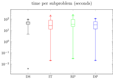
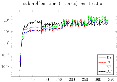
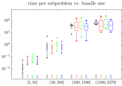
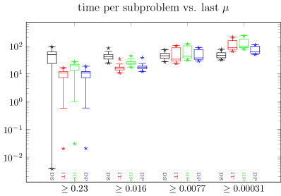
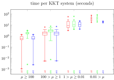
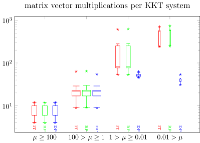
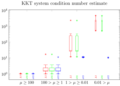
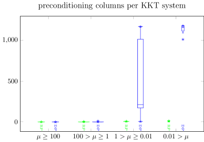
Figure 1: Instance MC, 338 subproblems, 2832 KKT systems. In order to highlight the dependence on the barrier parameter $\mu$ with corresponding precision requirements the results for KKT systems are grouped into $\mu$-value ranges $(\infty,100]$, $(100,1]$, $(1,0.01]$, $(0.01,0)$.

The graph was randomly generated ([35], call rudy -rnd_graph 20000 1 1 for 20000 nodes, edge density one percent, seed value 1). The semidefinite relaxation gives rise to an unconstrained problem with $20000$ variables. Each variable influences one of the diagonal elements of the Laplace matrix of the graph with cost one and the task is to minimize the maximum eigenvalue of the Laplacian times the number of nodes, see [25] for the general problem description.

For graphs of this type but smaller size like 5000 or 10000 nodes the direct solver DS still seemed to perform better, so rather large sizes are needed to see some advantage of iterative methods. Other than that the relative behavior of the solvers was similar also for the smaller sizes. The jaggies within subproblem time in the second plot are due to the reduction of the model to its active part after each descent step while the model typically increases in size during null steps. During the very first iterations the bundle is tiny and DS is the best choice. Once the bundle size increases sufficiently, the iterative methods dominate. Over time, as precision requirements get higher and the choice of the bundle subspace converges, the advantage of iterative methods decreases. In the final phase of high precision the direct solver may well be more attractive again.

The plots also show that for this instance (and presumably for most instances of this random type) the performance of IT (MINRES without preconditioning) is almost as good as DP (deterministic preconditioning) while RP (randomized preconditioning) is not competitive. Note that the condition number does not grow excessively for IT in this instance. Deterministic preconditioning succeeds in keeping the condition number almost exactly at the intended value 10. For smaller values of $\mu$, so for higher precision requirements, DP requires distinctly fewer matrix-vector multiplications, but it then also selects a large number of columns. In comparison to no preconditioning DP helps to improve stability but does not lead to significantly better computation times except maybe for the very last phase of the algorithm with high precision requirements.

4.2 Minimum Bisection (Instance BIS, Figure 2)

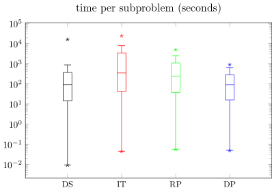
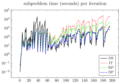
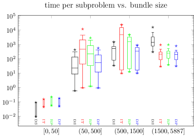
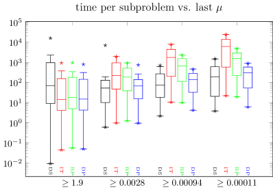
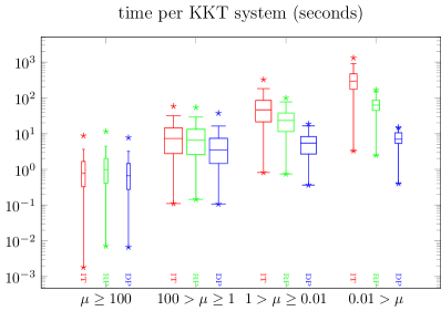
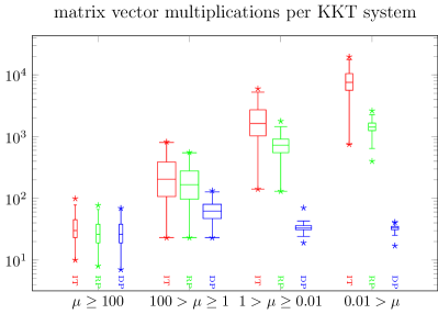
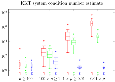
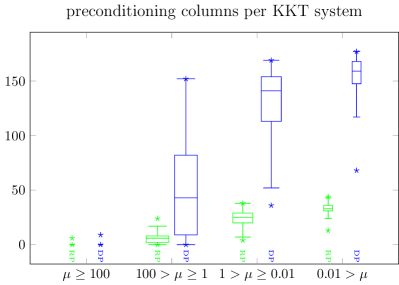
Figure 2: Instance BIS, 195 subproblems, 6180 KKT systems. In order to highlight the dependence on the barrier parameter $\mu$ with corresponding precision requirements the results for KKT systems are grouped into $\mu$-value ranges $(\infty,100]$, $(100,1]$, $(1,0.01]$, $(0.01,0)$.

The semidefinite relaxation of minimum bisection is similar in nature to max-cut, but in addition to the single diagonal elements there is a variable with coefficient matrix of all ones. Furthermore, variables with sparse coefficient matrices corresponding to odd cycles in the underlying graph are added dynamically in rounds, see [18] for the general framework and also for the origin of the instance KKT_traj33 with 20006 nodes and roughly 260000 edges.

Again, after the very first iterations the iterative methods turn out to perform distinctly better in the initial phase of the algorithm. Iterative methods get less attractive as precision requirements increase. The model size is often rather small (a bit larger than the active set of about 150 columns) which is favorable for DS. Indeed, additional output information of the log file indicates that the performance of DS drops off whenever the cutting model is significantly larger than that.

While for this instance RP is better than IT, the advantage of DP over the other iterative variants is quite apparent and its superiority also increases with precision requirements and smaller $\mu$. In fact, for DP the condition number and the number of matrix-vector multiplications decrease again for smaller $\mu$. Possible causes might be that the active set is easier to identify correctly. Due to the reduction in matrix-vector multiplications, computation time does not increase for DP in spite of a growing number of columns in the preconditioner.

4.3 A Min-Max-Bisection Problem (Instance MMBIS, Figure 3)

This problem arose in the context of an unpublished attempt to optimize vaccination rates for five population groups $N_{1}\dot{\cup}\dots\dot{\cup}N_{5}=N$ in a virtual town of $n=|N|$ inhabitants. Briefly, within the town $k$ anonymous people are assumed to be infectious. There is vaccine for at most $\underline{n}$ people. The aim is to reduce the spreading rate of the disease by vaccinating each person with the respective group’s probability. The task of determining these vaccination rates motivated the following ad hoc model which would be hard to justify rigorously. In a graph $G=(N,E)$ each edge $ij=\{i,j\}\in E$ with $i\in N_{\hat{\imath}}$, $j\in N_{\hat{\jmath}}$ has a weight $\hat{w}_{{\hat{\imath}}{\hat{\jmath}}}$ representing the infectiousness of the typical contact for these two persons of the respective groups. It will be convenient to define the weighted Laplacians $L_{{\hat{\imath}}{\hat{\jmath}}}=\hat{w}_{{\hat{\imath}}{\hat{\jmath}}}\sum_{ij\in E,i\in N_{\hat{\imath}},j\in N_{\hat{\jmath}}}(e_{i}-e_{j})(e_{i}-e_{j})^{\top}$. In this simplified approach, vaccination rates $v_{\hat{\imath}},v_{\hat{\jmath}}$ of the node groups reduce a nominal infectiousness $\hat{w}_{{\hat{\imath}}{\hat{\jmath}}}$ between these groups by the factor $y_{{\hat{\imath}}{\hat{\jmath}}}\geq\max\{0,1-v_{\hat{\imath}}-v_{\hat{\jmath}}\}$. The spreading probability to be minimized is considered proportional to the restricted max-cut value

$$\displaystyle\max_{{\mathcal{I}}\subset N,|{\mathcal{I}}|=k}\sum y_{{\hat{\imath}}{\hat{\jmath}}}\hat{w}_{{\hat{\imath}}{\hat{\jmath}}}\cdot|\{ij\in E\colon i\in{\mathcal{I}}\cap N_{\hat{\imath}},j\in N_{\hat{\jmath}}\setminus{\mathcal{I}}\}|=$$

$$=\displaystyle\max_{x\in\{-1,1\}^{n}\atop(\mathbbm{1}^{\top}x)^{2}=(n-2k)^{2}}\frac{1}{4}x^{\top}\bigg{(}\sum_{{\hat{\imath}}\leq{\hat{\jmath}}}y_{{\hat{\imath}}{\hat{\jmath}}}L_{{\hat{\imath}}{\hat{\jmath}}}\bigg{)}x,$$

For determining the vaccination rates the combinatorial problem is replaced by the usual (dual) semidefinite relaxation

$$\begin{array}[]{rl}\text{minimize}&\frac{n}{4}\lambda_{\max}(\sum_{{\hat{\imath}}\leq{\hat{\jmath}}}y_{{\hat{\imath}}{\hat{\jmath}}}L_{{\hat{\imath}}{\hat{\jmath}}}-\mathop{\rm Diag}(d)-u\mathbbm{1}\mathbbm{1}^{\top})+\mathbbm{1}^{\top}d+(n-2k)^{2}u\\ \text{subject to}&y_{{\hat{\imath}}{\hat{\jmath}}}\geq 1-v_{\hat{\imath}}-v_{\hat{\jmath}},\qquad{\hat{\imath}}\leq{\hat{\jmath}},\\ &\sum_{{\hat{\imath}}}|N_{\hat{\imath}}|v_{\hat{\imath}}=\underline{n},\\ &d\in\mathbb{R}^{n},u\in\mathbb{R},y\geq 0,v\geq 0.\end{array}$$

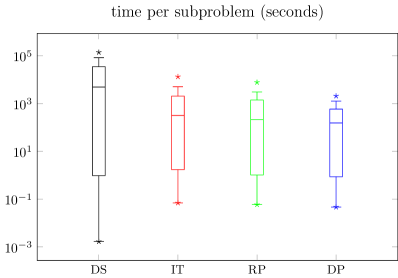
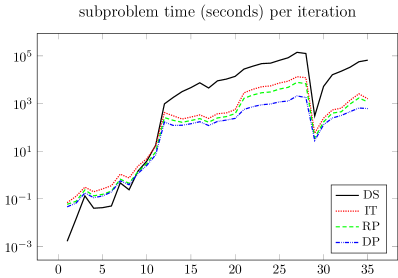
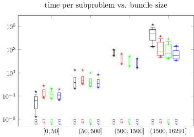
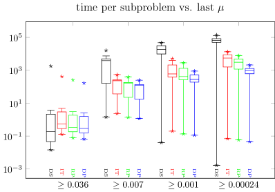
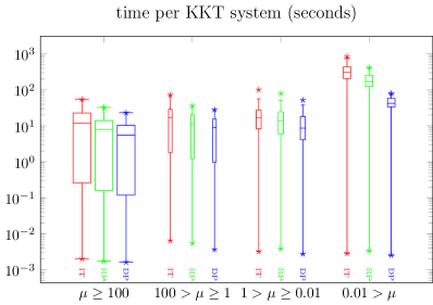
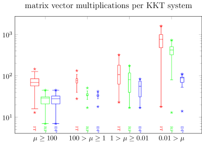
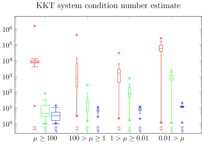
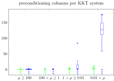
Figure 3: Instance MMBIS, 35 subproblems, 782 KKT systems. In order to highlight the dependence on the barrier parameter $\mu$ with corresponding precision requirements the results for KKT systems are grouped into $\mu$-value ranges $(\infty,100]$, $(100,1]$, $(1,0.01]$, $(0.01,0)$.

In this case the resulting KKT system also has an equality and several inequality constraints in the block $A$. Preconditioning results are presented for the KKT systems of an instance with $n=12600$ inhabitants splitting into groups of sizes $5770,6000,600,30,200$, with $k=126$ infectious persons and $\underline{n}=1260$ available vaccinations.

In the actual computations the bundle size grows surprisingly fast. This not only entails enormous memory requirements but also excessive computation times for DS; indeed, computations of DS may exceed those of DP by a factor of 70. In consequence comparative results can only be reported for a very limited number of subproblem evaluations. In particular, the precision requirements remain rather moderate throughout these iterations. Still, the same initial behavior can be observed as for the previous two instances. For very small bundle sizes DS is best. Once the bundle size grows, the iterative methods take over. Among the iterative solvers RP is better than IT, but DP is the method of choice. It succeeds in tightly controlling the condition number by selecting rather few columns. With this DP requires the fewest matrix vector multiplications which seems to pay of quickly on this instance.

4.4 Performance within the Bundle Method for Max-Cut

The purpose of this section is to provide evidence for the reliability of the KKT oriented evaluations when the iterative solvers are employed within the bundle method directly. As explained in the introductory remarks to this Section 4, a full assessment of the use of iterative solvers within conic bundle methods is out of scope and beyond the possibilities of this work. Therefore results will only compare, without any further adaptations, the direct replacement of DS with the solvers IT, RP and DP, within the current ConicBundle implementation that was developed and tuned for DS. Note, however, that the evaluation of bundle methods requires a statistical approach.

In oracle based nonsmooth optimization it is typical that even slight numerical changes in the computation of candidates bring along significant differences in the actual trajectories. Indeed, candidates are generically close to ridges. Which subgradient is returned depends on which side of the ridge the candidate ends up. In particular, the use of different KKT solvers quickly leads to considerable differences in the models and subproblems and therefore also in the sequence of KKT problems. This erratic behavior is intrinsic at any level of precision, therefore it may be expected that the average number of bundle iterations (descent and null steps) does not depend too much on the actual KKT solver in use. Yet, due to this incomparability of trajectories, any attempt to assess the scope of the iterative solvers in comparison to the direct solver needs to be based on a reasonable collection of comparable instances. Their choice should help to illustrate the effects of parameters, that can be expected to be influential in the current context,

• the cost of matrix-vector multiplications,

• the size of the model,

• precision requirements,

• the use or non-use of a predictor corrector approach,

• the number of KKT instances and solves per subproblem.

In order to cover these aspects with manageable effort, results will be presented for eight methods and four groups of 25 randomly generated Max-Cut instances. The methods without predictor corrector approach are denoted by DS, IT, RP, DP and those with predictor corrector approach by DSp, ITp, RPp, DPp. The names refer to using the respective direct or iterative solver for the KKT systems of the internal interior point method of ConicBundle for solving the subproblems. The four instance classes arise by generating five instances per number of nodes $n\in\{10000,20000\}$ and per density out of two edge density groups, one with smaller densities $d\in\{0.1,0.2,0.3,0.4,0.5\}$ and one with higher density $d\in\{1,2,3,4,5\}$ ([35], call rudy -rnd_graph n d s for seed $s\in\{1,2,3,4,5\})$. The instances were solved with ConicBundle [19] on computers having QUAD-Core-processors INTEL-Core-I7-4770 with 4$\times$ 3400MHz, 8 MB Cache, 32 GB RAM and operating system Ubuntu 18.04. The code was run in sequential mode with each instance solved en suite for all methods on the same machine and all time measurements refer to user time. Mandated by limited resources, some volatility may have been caused by running two instances on each machine at the same time as well as by occasional further jobs. As instances and methods were randomly affected by this, influence on the conclusions should be marginal in view of the number of examples.

The max-cut instances serve the purpose well for the following reasons. First, as explained before, the direct solver DS is particularly efficient for Max-Cut instances, because the Schur complement needs to be computed only once at the beginning of each bundle step for all interior point iterations / KKT systems associated with this subproblem. Thus, if iterative solvers are competitive for Max-Cut this should also hold for more general cases. Likewise, the iterative solver IT without preconditioning performed better on the KKT instances for Max-Cut than on those of the two other examples, therefore the limits of preconditioning are best discussed for Max-Cut. Second, for Max-Cut even large scale instances can be solved to reasonably high precision in manageable time which allows to compare the performance on several precision levels. To make this comparison reasonably efficient and fair in view of the weaknesses of the lack of progress stopping criterion of bundle methods, the comparisons use for each level of relative precision $10^{-3}$, $10^{-4}$, $10^{-5}$ and $10^{-6}$ the first descent step that produces a value below an instance dependent common relative reference value. For each instance this reference value is obtained by taking the minimum objective value obtained over all methods by running ConicBundle with termination precision $10^{-6}$. Third, random max-cut instances having the same number of nodes and similar edge density can be expected to have similar parameters and properties in terms of model size, cost of matrix-vector multiplications, and precision requirements. Note that a higher edge density increases the cost of matrix-vector multiplications but also causes a larger offset in objective value which entails somewhat reduced precision requirements for the KKT systems to reach the same relative precision. As the experiments will show, the model size — it is selected by ConicBundle on basis of the active rank, starts with roughly twice this size after descent steps for reasons investigated in [10] and increases further over null steps — seems to be less dependent on the edge densities but grows markedly with the number of nodes.

Development of subproblem / bundle step parameters for the 10000 node instances density $\in\{0.1,0.2,0.3,0.4,0.5\}$ density $\in\{1,2,3,4,5\}$

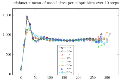
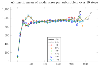
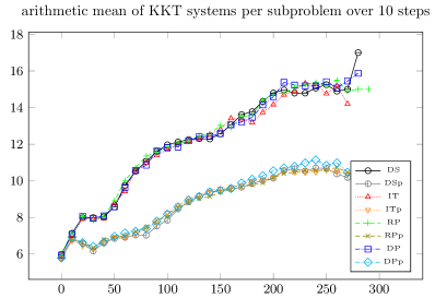
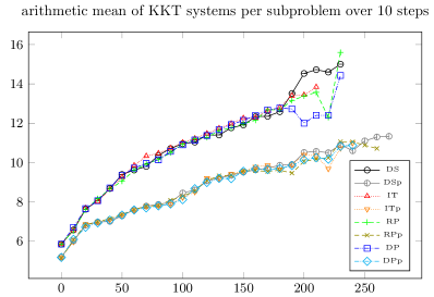
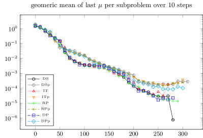
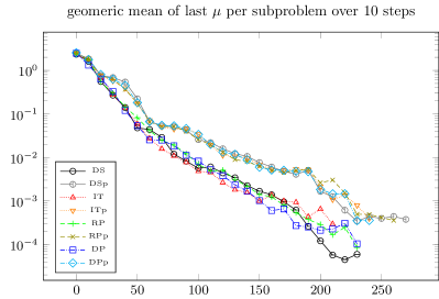
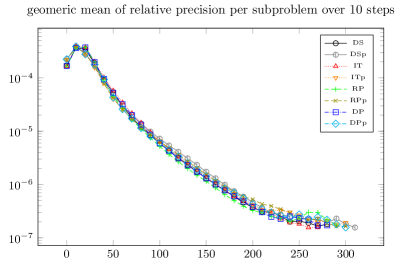
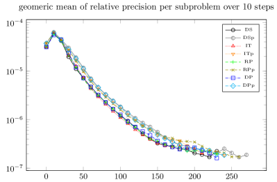
Figure 4: The plots show for each method for successive groups of 10 bundle iterations (null or descent steps) over all instances the arithmetic mean of the model size and of the number of interior point iterations of the subproblems in this group and the geometric mean of the last $\mu$ value and of the relative precision the interior point method needed to reach. All iterations of the performance profile for relative precision level $10^{-6}$ are included.

Development of subproblem / bundle step parameters for the 20000 node instances density $\in\{0.1,0.2,0.3,0.4,0.5\}$ density $\in\{1,2,3,4,5\}$

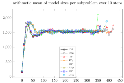
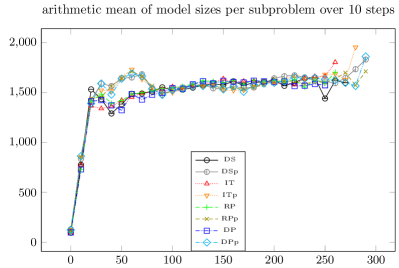
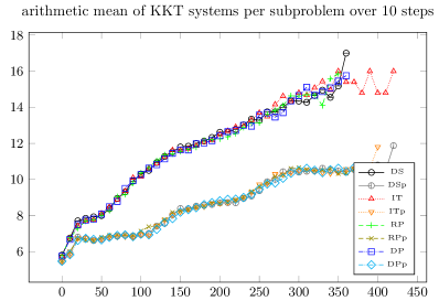
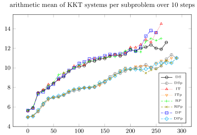
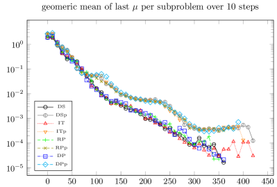
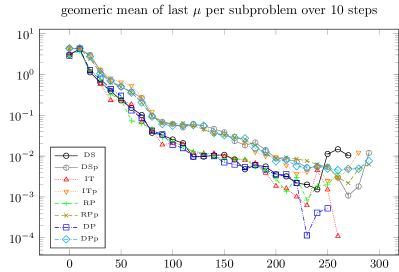
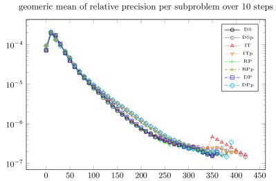
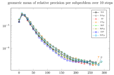
Figure 5: The plots show for each method for successive groups of 10 bundle iterations (null or descent steps) over all instances the arithmetic mean of the model size and of the number of interior point iterations of the subproblems in this group and the geometric mean of the last $\mu$ value and of the relative precision the interior point method needed to reach. All iterations of the performance profile for relative precision level $10^{-6}$ are included.

The first aspect to address is the dependence of the bundle method on the solvers. For this figures 4 and 5 display for each group and solver the average development of the model sizes, the number of KKT systems solved per subproblem together with the last $\mu$-value occuring there (it reflects the precision requirement of the final KKT system within the subproblem) and also the precision requirements on the subproblems themselves. This development is recorded in averages over groups of 10 steps and all 25 instances for each of the four instance groups. This rather detailed view will also help to explain differences in the computation times of the solvers for various precision levels.

Performance profiles of bundle steps and KKT systems for sparser 20000 node instances

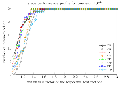
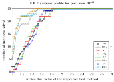
Figure 6: The performance profiles are generated for the 20000 node instances having densities in $\{0.1,0.2,0.3,0.4,0.5\}$ with respect to the total number of bundle iterations (null and descent steps) [left] and the total sum of KKT systems over all subproblems [right] needed to reach a relative precision of $10^{-6}$ relative to the best value obtained over all methods.

The plots of figures 4 and 5 exhibit a natural separation between the methods with and without predictor corrector approach. In comparison, the differences between the solvers are almost negligible except for a few final iterations, which also suffer from stronger volatility due to a reduced number of samples. It is worth noting that the same holds for the overall number of KKT systems and bundle steps throughout all relative precision levels. A helpful visualization to illustrate such comparisons are performance profiles [11] for the total number of steps and KKT systems for each precision level. These turn out to have a shape similar to that displayed in Figure 6 which presents the two profiles for bundle steps and KKT systems for the sparser case on 20000 nodes and relative precision $10^{-6}$. While the smaller number of KKT systems (i.e. interior point iterations) of the predictor corrector variants is an expected outcome, it is rather surprising that the variants without predictor corrector seem to need a few bundle steps less on average to reach the required precision. A comparison with the model size plots of 4 and 5 suggests, that there is a distinct difference in the nature of these interior point solutions that also has its effect on the bundle selection mechanism, but so far this lacks a mathematically sound explanation. Still, a first conclusion might read that the behavior of the bundle method itself is, on average, independent of the choice of the four solvers.

Time performance profiles for max-cut on 10000 nodes with 5 instances per 5 densities density $\in\{0.1,0.2,0.3,0.4,0.5\}$ density $\in\{1,2,3,4,5\}$

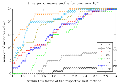
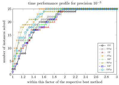
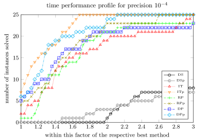
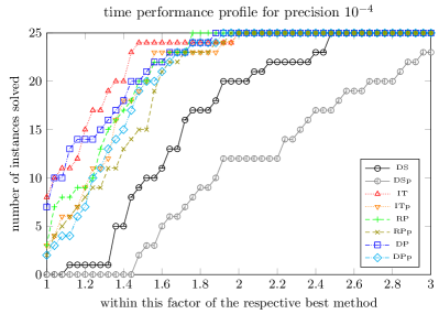
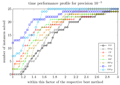
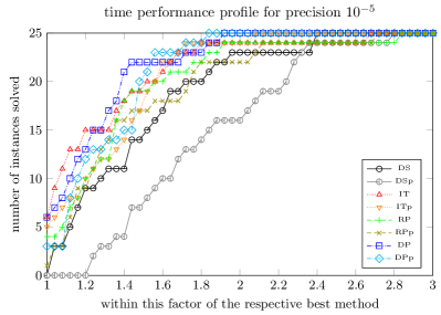
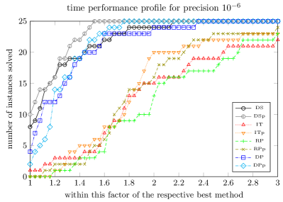
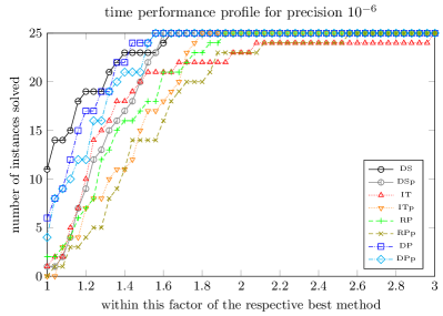
Figure 7: The profile is taken with respect to the time needed to reach a relative precision of $10^{-3}$, $10^{-4}$, $10^{-5}$, and $10^{-6}$ relative to the best value obtained over all methods.

Time performance profiles for max-cut on 20000 nodes with 5 instances per 5 densities density $\in\{0.1,0.2,0.3,0.4,0.5\}$ density $\in\{1,2,3,4,5\}$

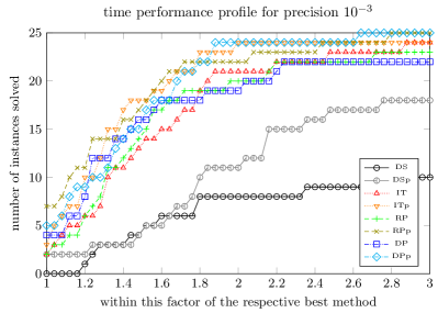
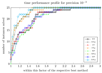
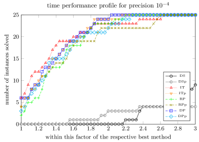
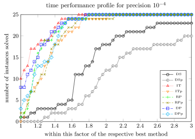
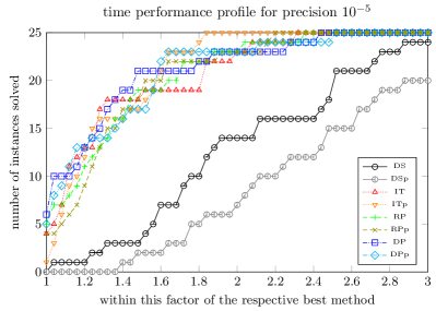
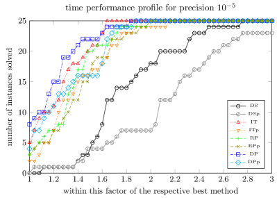
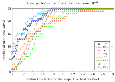
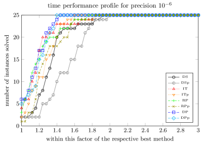
Figure 8: The profile is taken with respect to the time needed to reach a relative precision of $10^{-3}$, $10^{-4}$, $10^{-5}$, and $10^{-6}$ relative to the best value obtained over all methods.

Figures 7 and 8 display computation time performance profiles of the eight methods on the four classes of 25 instances for relative precision levels $10^{-3}$, $10^{-4}$, $10^{-5}$ and $10^{-6}$. These largely match the results on individual KKT systems. First consider the direct solvers DS and DSp. Again, a good explanation is lacking for the fact that DS dominates DSp in many cases with higher number of edges and higher precision. Whether DS and DSp are attractive compared to iterative methods depends on the ratio of the time invested into forming the Schur complement to the number of KKT steps required for solving the subproblem, i. e., they are preferable if the model size is small or the number of interior point iterations becomes large enough due to increasing precision requirements. In cases of strong initial growth of the model size (see the model size plots of figures 4 and 5) iterative solvers are quickly better. The seemingly good performance of the direct solvers on the denser instances for precision level $10^{-3}$ is mostly due to the large constant offset that causes the methods to reach this precision often within ten steps (compare this to the asymptotic analysis in [21]); at this point model sizes are still small. Iterative solvers dominate precision levels $10^{-4}$ and $10^{-5}$ with reasonably low accuracy and few interior point iterations. The influence of the cost of a matrix-vector multiplication is visible in the difference of the initial head start to direct solvers between sparser and denser instances for precision $10^{-4}$. For instances on 20000 nodes the average model size is one and a half times the average size of the 10000 node instances (see figures 4 and 5)) and this explains part of the stronger performance of the iterative solvers on larger instances. For increasing precision requirements and number of interior point iterations the profiles also suggest that DS and DSp catch up faster for instances with fewer edges. This effect might again be caused by the constant offset, that is larger for random Max-Cut instances with larger number of edges. Indeed, an inspection of the last $\mu$ plots and KKT systems per subproblem in figures 4 and 5 suggests that for max-cut instances with a larger number of edges the subproblem solutions require less absolute accuracy which favors iterative solvers and compensates somewhat the higher cost of the matrix-vector multiplications. Note that the relative precision requirements for the solution of the subproblems (see figures 4 and 5) are almost identical.

For the iterative methods the predictor corrector variant seems faster on lower precision levels but again the methods without predictor corrector catch up or may even dominate higher precision levels. For IT (no preconditioning) this should largely be due to the fact that predictor corrector requires two solves per KKT system. Thus, taking twice the number of KKT systems per problem for predictor corrector variants in figures 4 and 5 as the number of required solves provides a satisfactory explanation for IT. For RP and DP the situation is less clear cut, because the preconditioner is formed only once per KKT system, but the line of argument is similar. For the moderate accuracy levels $10^{-3}$ and $10^{-4}$ Max-Cut instances could do without preconditioning, but the preconditioned variants do a good job. For $10^{-5}$ the advantage begins to show and for $10^{-6}$ the DP variants are almost consistently better than the other iterative methods.

Based on this analysis, a hybrid approach seems advisable that switches dynamically between the solvers depending on precision, model size and number of interior point iterations. In implementing these ideas a number of further design aspects would have to be reconsidered as outlined before. The true advantage of iterative solvers, however, is that dynamic model adaptations become feasible during the solution of the subproblem, because there is no need to recompute the Schur complement each time. This allows for entirely new strategies such as combining the ideas of [33, 4] and [24] in order to cut down on the number null steps at an early stage. This remains to be addressed in future work.

5 Conclusions

In search for efficient low rank preconditioning techniques for the iterative solution of the internal KKT system of the quadratic bundle subproblem two subspace selection heuristics — a randomized and a deterministic variant — were proposed. For the randomized approach the results are ambivalent in theory and in practice; obtaining a good subspace this way seems to be difficult and the cost of exploratory matrix-vector multiplications quickly dominates. In contrast, the deterministic subspace selection approach allows to control the condition number (and with it the number of matrix vector multiplications) at a desired level without the need to tune any parameters in theory as well as on the test instances. On these instances, for low precision requirements (large barrier parameter) the selected subspace is negligible small. For high precision requirements (small barrier parameter) the subspace grows to the active model subspace. If the bundle size is close to this active dimension, the work in forming the preconditioner may be comparable to forming the Schur complement for the direct solver. Still, for large scale instances the deterministically preconditioned iterative approach seems to be preferable.

Conceivably it is possible to profit in ConicBundle from the advantages of the deterministic iterative and the direct solver by switching dynamically between both. The current experiments relied on a predictor-corrector approach that was tuned for the direct solver. In view of the properties of the iterative approach it may well be worth to devise a different path following strategy for the iterative approach, in particular for the initial phase of the interior point method when the barrier parameter is still comparatively large and the work invested in forming the preconditioner is still negligible. Similar ideas should be applicable to interior point solvers for solving convex quadratic problems with low rank structure.

Acknowledgments I have profited a lot from discussions with many colleagues, in part years back. In particular I have to thank K.-C. Toh as well as my colleagues O. Ernst, R. Herzog, A. Pichler and M. Stoll in Chemnitz. Much of the preparatory restructuring of ConicBundle was done during my sabbatical at the University of Klagenfurt, thank you to F. Rendl and A. Wiegele for making this possible. The support of research grants 05M18OCA of the German Federal Ministry of Education and Research and the DFG CRC 1410 is gratefully acknowledged.

Appendix A Tables

For each box plot of figures 1–3 for the three instances MC, BIS and MMBIS the following tables list the number of instances and the values of the parameters minimum, lower quartile ($Q_{1}$), median, upper quartile ($Q_{3}$), maximum. For each of the three instances an additional table gives the statistics on the Euclidean norm of the resulting residual of (6) achieved by the respective solver for the KKT systems grouped by the usual value ranges of the barrier parameter.

A.1 Max-Cut (Instance MC, Figure 1)

Time per subproblem in seconds (338 instances):

solver min $Q_{1}$ median $Q_{3}$ max DS 0.003832 34.3212 44.6572 55.9219 95.1265 IT 0.020491 12.6342 26.1729 79.1747 209.58 RP 0.030548 22.0347 34.3771 92.207 235.653 DP 0.020898 13.0997 30.6566 58.1994 110.33

Time per subproblem in seconds vs. ranges of bundle sizes:

bundle size # solver min $Q_{1}$ median $Q_{3}$ max $[6,46]$ 5 DS 0.003832 0.006275 0.0088455 0.021121 0.045992 IT 0.020491 0.021558 0.031059 0.059577 0.095407 RP 0.030548 0.0314005 0.043048 0.093556 0.146144 DP 0.020898 0.0230755 0.0309575 0.0592245 0.094453 $[56,497]$ 5 DS 0.073058 0.329229 0.657365 1.0668 4.51608 IT 0.173868 0.374044 0.597913 0.800166 1.83209 RP 0.273307 0.637968 1.02498 1.4059 3.19528 DP 0.177225 0.382114 0.59731 0.80289 1.6773 $[596,1486]$ 133 DS 6.62451 30.4929 33.6252 36.9311 43.6407 IT 1.86562 12.7032 25.3882 65.6882 136.935 RP 3.69818 20.2136 33.3548 77.6126 155.415 DP 1.96853 13.9917 30.0676 49.426 90.8324 $[1541,2279]$ 195 DS 41.2984 46.7501 53.9483 61.8286 95.1265 IT 9.84382 13.6284 32.0618 90.4042 209.58 RP 18.53 23.4963 42.6607 106.814 235.653 DP 9.9354 13.9977 36.494 76.5581 110.33

Time per subproblem in seconds vs. last barrier parameter $\mu$:

$\mu$-range # solver min $Q_{1}$ median $Q_{3}$ max $[2.3e-01,3.6e+01]$ 85 DS 0.003832 23.4027 49.1143 61.5018 95.1265 IT 0.020491 7.2764 10.8231 11.9651 16.4467 RP 0.030548 13.4739 19.5347 22.0031 27.3839 DP 0.020898 7.2377 10.8421 11.9242 18.6599 $[1.6e-02,2.3e-01]$ 85 DS 24.2787 33.6785 41.3086 48.8582 83.315 IT 10.8004 13.7717 15.5724 17.2952 33.9445 RP 17.3893 22.0349 24.1102 27.3977 44.4086 DP 12.0901 15.1287 17.2843 18.8158 37.7594 $[7.7e-03,1.6e-02]$ 85 DS 26.8515 35.9349 44.6111 54.1812 73.3521 IT 23.8603 28.455 33.4883 86.0521 103.067 RP 30.9349 37.0011 43.6655 100.814 120.387 DP 28.6909 32.9195 37.3972 74.0808 87.0083 $[3.1e-04,7.7e-03]$ 83 DS 31.4011 37.4751 45.8135 57.0963 75.7966 IT 64.8852 75.3411 87.3138 154.968 209.58 RP 77.5913 87.3499 99.7462 175.749 235.653 DP 49.3655 53.8412 62.3306 96.8023 110.33

Time per KKT system in seconds grouped by value ranges of the barrier parameter $\mu$:

$\mu$-range # solver min $Q_{1}$ median $Q_{3}$ max $[4.5e+02,9.9e+02]$ 676 IT 0.001092 0.463337 0.578703 0.917693 1.34934 RP 0.002696 1.54367 1.80541 2.1684 3.22664 DP 0.00252 0.515255 0.630482 0.916957 1.37408 $[1.4e+00,5.1e+01]$ 1490 IT 0.005506 1.2121 1.83286 2.31178 6.49419 RP 0.007486 2.36829 3.09237 3.69645 7.72418 DP 0.005681 1.22031 1.82556 2.29723 7.32683 $[1.6e-02,3.1e-01]$ 510 IT 3.20468 5.69856 8.79662 21.8884 56.4563 RP 4.19829 6.85746 10.4541 23.0927 60.4059 DP 4.28737 7.03695 10.7758 18.0144 23.1913 $[3.1e-04,9.3e-03]$ 156 IT 17.2603 22.94 37.6166 52.734 74.6325 RP 19.0854 25.2808 40.9692 55.18 82.3144 DP 16.0158 18.3264 19.1491 19.8728 22.2577

Number of matrix vector multiplications per KKT system grouped by value ranges of $\mu$:

$\mu$-range # solver min $Q_{1}$ median $Q_{3}$ max $[4.5e+02,9.9e+02]$ 676 IT 4 6 6 10 12 RP 4 6 6 10 12 DP 4 6 6 10 12 $[1.4e+00,5.1e+01]$ 1490 IT 9 17 22 23 64 RP 9 17 22 23 64 DP 9 17 22 23 55 $[1.6e-02,3.1e-01]$ 510 IT 54 77 84 252 612 RP 54 77 84 253 627 DP 45 49 52 54 63 $[3.1e-04,9.3e-03]$ 156 IT 240 248 550 574 706 RP 249 253 574 592 739 DP 31 37 38 42 54

Condition number estimate of the KKT systems grouped by value ranges of $\mu$:

$\mu$-range # solver min $Q_{1}$ median $Q_{3}$ max $[4.5e+02,9.9e+02]$ 676 IT 1.003 1.009 1.009 1.01 1.065 RP 1.003 1.009 1.009 1.01 1.065 DP 1.003 1.009 1.009 1.01 1.065 $[1.4e+00,5.1e+01]$ 1490 IT 1.013 1.473 1.566 2.393 17.06 RP 1.013 1.473 1.566 2.393 16.98 DP 1.013 1.473 1.566 2.393 11.38 $[1.6e-02,3.1e-01]$ 510 IT 12.03 26.72 29.72 253.7 2349 RP 11.87 26.44 29.33 250.7 2289 DP 10.62 11.11 11.46 11.75 11.96 $[3.1e-04,9.3e-03]$ 156 IT 523.5 536.4 2057 2404 4711 RP 507.1 527.3 2017 2371 4599 DP 10.17 10.43 10.56 10.66 10.93

Number of preconditioning columns per KKT system grouped by value ranges of $\mu$:

$\mu$-range # solver min $Q_{1}$ median $Q_{3}$ max $[4.5e+02,9.9e+02]$ 676 RP 0 0 0 0 0 DP 0 0 0 0 0 $[1.4e+00,5.1e+01]$ 1490 RP 0 0 0 0 6 DP 0 0 0 0 12 $[1.6e-02,3.1e-01]$ 510 RP 6 6 6 6 8 DP 5 171 212 1012 1167 $[3.1e-04,9.3e-03]$ 156 RP 7 8 10 10 13 DP 1010 1113 1156 1175 1177

Euclidean norm of the residual of (6) per KKT system grouped by value ranges of $\mu$:

$\mu$-range # solver min $Q_{1}$ median $Q_{3}$ max $[4.5e+02,9.9e+02]$ 676 IT 6.4e-10 1.4e-09 2.6e-09 5.2e-09 1e-06 RP 6.4e-10 1.4e-09 2.6e-09 5.2e-09 1e-06 DP 6.4e-10 1.4e-09 2.6e-09 5.2e-09 1e-06 $[1.4e+00,5.1e+01]$ 1490 IT 3.6e-10 6.7e-09 5.2e-08 3.9e-07 1e-06 RP 3.6e-10 6.4e-09 5.2e-08 3.9e-07 1.1e-06 DP 3.6e-10 6.7e-09 5.2e-08 3.9e-07 1e-06 $[1.6e-02,3.1e-01]$ 510 IT 8.6e-09 7e-07 8.2e-07 9.2e-07 1e-06 RP 9.7e-09 7.3e-07 9.2e-07 1.1e-06 2.4e-06 DP 5.2e-09 5.4e-07 6.8e-07 7.9e-07 1.2e-06 $[3.1e-04,9.3e-03]$ 156 IT 9.7e-09 9.6e-07 9.8e-07 9.9e-07 1e-06 RP 1.9e-08 1.4e-06 2.2e-06 4.2e-06 6.2e-06 DP 8.6e-09 5.8e-07 7.1e-07 8.1e-07 1e-06

A.2 Minimum Bisection (Instance BIS, Figure 2)

Time per subproblem in seconds (195 instances):

solver min $Q_{1}$ median $Q_{3}$ max DS 0.00923 14.1723 91.7467 359.175 15841.2 IT 0.044218 42.3879 340.967 3329.25 24016.1 RP 0.055209 36.3358 238.703 1079.8 4866.25 DP 0.049162 15.9154 89.9136 277.508 890.086

Time per subproblem in seconds vs. ranges of bundle sizes:

bundle size # solver min $Q_{1}$ median $Q_{3}$ max $[6,28]$ 2 DS 0.00923 – 0.00923 – 0.091545 IT 0.044218 – 0.044218 – 0.153935 RP 0.055209 – 0.055209 – 0.222727 DP 0.049162 – 0.049162 – 0.177788 $[67,497]$ 128 DS 0.594552 8.69331 22.7682 132.809 428.513 IT 0.960953 43.8529 466.297 2076.04 11867 RP 1.23022 33.9205 219.14 835.573 2856.49 DP 0.941817 11.8932 53.3373 183.946 560.093 $[529,1379]$ 40 DS 34.3749 81.2278 517.036 720.019 1505.5 IT 9.82356 16.6676 4819.87 15092.7 24016.1 RP 12.5897 20.357 1586.65 3277.46 4866.25 DP 10.0625 16.2665 340.397 612.94 890.086 $[1597,5887]$ 25 DS 302.944 783.079 1403.96 3335.16 15841.2 IT 29.3698 85.8307 211.467 294.115 932.896 RP 38.2829 108.971 248.069 341.147 955.341 DP 31.1555 87.6845 204.633 295.527 789.044

Time per subproblem in seconds vs. last barrier parameter $\mu$:

$\mu$-range # solver min $Q_{1}$ median $Q_{3}$ max $[1.9e+00,1.0e+03]$ 49 DS 0.00923 8.97908 69.8681 955.047 15841.2 IT 0.044218 4.08472 14.083 154.701 932.896 RP 0.055209 4.93747 18.2564 178.33 955.341 DP 0.049162 4.21385 14.8836 143.015 789.044 $[2.8e-03,1.4e+00]$ 49 DS 0.594552 9.95126 52.3298 128.666 6981.47 IT 0.960953 46.9621 218.946 937.902 1927.16 RP 1.23022 38.2691 183.586 508.265 933.538 DP 0.941817 15.3137 66.5916 139.005 734.869 $[9.4e-04,2.8e-03]$ 49 DS 2.12836 18.2489 73.8103 267.252 705.689 IT 10.3255 198.11 1744.97 4383.54 7789.69 RP 9.92439 111.622 670.068 1522.76 2315.44 DP 4.13901 32.1878 138.761 282.768 459.79 $[1.1e-04,9.4e-04]$ 48 DS 3.77535 20.2483 189.134 599.782 1505.5 IT 21.8778 575.065 6101.11 13836.1 24016.1 RP 19.1305 219.14 1524.83 2942.66 4866.25 DP 5.98724 52.4419 299.974 580.588 890.086

Time per KKT system in seconds grouped by value ranges of the barrier parameter $\mu$:

$\mu$-range # solver min $Q_{1}$ median $Q_{3}$ max $[1.1e+02,2.6e+04]$ 824 IT 0.001823 0.328123 0.786603 1.66599 8.7638 RP 0.007159 0.410637 0.980222 2.023 11.5388 DP 0.006695 0.275799 0.669313 1.45762 7.73375 $[1.0e+00,9.9e+01]$ 2262 IT 0.110818 2.7715 7.29372 14.4584 58.5776 RP 0.145002 2.60334 6.57376 13.2324 54.0312 DP 0.10742 1.46962 3.4827 7.40111 37.485 $[1.0e-02,1.0e+00]$ 1991 IT 0.817783 21.4256 46.2355 85.6325 327.564 RP 0.744242 11.4276 23.3757 37.8191 100.053 DP 0.365208 2.70049 5.41858 8.25427 18.679 $[1.1e-04,1.0e-02]$ 1103 IT 3.30796 173.717 295.614 470.923 1316.81 RP 2.48871 44.4168 62.784 86.7278 168.322 DP 0.40273 5.37352 6.99157 10.5791 14.8519

Number of matrix vector multiplications per KKT system grouped by value ranges of $\mu$:

$\mu$-range # solver min $Q_{1}$ median $Q_{3}$ max $[1.1e+02,2.6e+04]$ 824 IT 10 23 30 45 99 RP 8 19 26 38 77 DP 7 19 26 38 69 $[1.0e+00,9.9e+01]$ 2262 IT 23 107 204 386.5 820 RP 23 97 166 277 555 DP 23 47 62 80 133 $[1.0e-02,1.0e+00]$ 1991 IT 141 1024.5 1632 2719.5 5960 RP 130 548.5 722.5 910.5 1774 DP 19 31 33 36 70 $[1.1e-04,1.0e-02]$ 1103 IT 750 5607.5 7552.5 10475 19571 RP 399 1249 1419.5 1657 2620 DP 17 31 33 35 41

Condition number estimate of the KKT systems grouped by value ranges of $\mu$:

$\mu$-range # solver min $Q_{1}$ median $Q_{3}$ max $[1.1e+02,2.6e+04]$ 824 IT 2.15 3.773 5.36 12.1 997.8 RP 1.008 2.465 3.84 7.696 67.38 DP 1.122 2.469 3.834 7.442 25.34 $[1.0e+00,9.9e+01]$ 2262 IT 3.681 93.22 277.5 1041 1.234e+04 RP 2.035 59.19 160 477 2544 DP 2.035 7.361 15.99 27.31 407.7 $[1.0e-02,1.0e+00]$ 1991 IT 289.5 1.409e+04 4.986e+04 1.869e+05 2.075e+06 RP 246.8 3107 6609 1.405e+04 9.741e+04 DP 1.717 2.29 2.632 3.128 27.66 $[1.1e-04,1.0e-02]$ 1103 IT 4.501e+04 1.324e+06 2.869e+06 6.53e+06 4.576e+07 RP 7554 3.375e+04 5.161e+04 8.013e+04 4.099e+05 DP 1.703 2.048 2.185 2.522 12.55

Number of preconditioning columns per KKT system grouped by value ranges of $\mu$:

$\mu$-range # solver min $Q_{1}$ median $Q_{3}$ max $[1.1e+02,2.6e+04]$ 824 RP 0 0 0 0 6 DP 0 0 0 0 9 $[1.0e+00,9.9e+01]$ 2262 RP 0 2 6 8 24 DP 0 9 43 82 152 $[1.0e-02,1.0e+00]$ 1991 RP 4 20 25 29 38 DP 36 113 141 154 169 $[1.1e-04,1.0e-02]$ 1103 RP 13 31 33 36 44 DP 68 147.5 159 168 177

Euclidean norm of the residual of (6) per KKT system grouped by value ranges of $\mu$:

$\mu$-range # solver min $Q_{1}$ median $Q_{3}$ max $[1.1e+02,2.6e+04]$ 824 IT 9.8e-13 9.1e-09 3.2e-07 5.6e-07 1e-06 RP 1.4e-12 6.9e-09 1.9e-07 3.5e-07 1.7e-06 DP 1.3e-12 7e-09 1.9e-07 3.5e-07 1.1e-06 $[1.0e+00,9.9e+01]$ 2262 IT 2.9e-10 4.7e-09 6.7e-09 5e-07 1e-06 RP 3.1e-10 4e-09 5.7e-09 3.3e-07 3.2e-06 DP 3.8e-10 5e-09 7.4e-09 3.5e-07 2.8e-06 $[1.0e-02,1.0e+00]$ 1991 IT 1.2e-09 5e-09 9e-09 1.9e-08 1e-06 RP 1.6e-09 6.4e-09 1.2e-08 2.4e-08 2.2e-05 DP 6.6e-10 5.2e-09 9.4e-09 2e-08 7.2e-06 $[1.1e-04,1.0e-02]$ 1103 IT 4.3e-09 4.9e-08 1.1e-07 3.3e-07 2.9e-06 RP 3.5e-09 3.3e-08 5.7e-08 9.5e-08 7.3e-05 DP 2.2e-09 3.4e-08 6e-08 1e-07 5.3e-06

A.3 Min-Max Bisection (Instance MMBIS, Figure 3

Time per subproblem in seconds (35 instances):

solver min $Q_{1}$ median $Q_{3}$ max DS 0.001669 0.958311 4942 35185.7 140651 IT 0.06925 1.7246 319.124 2069.75 13368.7 RP 0.059093 1.02453 215.038 1412.83 7763.78 DP 0.046371 0.864647 154.628 590.86 2083.68

Time per subproblem in seconds vs. ranges of bundle sizes:

bundle size # solver min $Q_{1}$ median $Q_{3}$ max $[0,37]$ 7 DS 0.001669 0.008018 0.0415445 0.091635 0.240095 IT 0.06925 0.098375 0.229849 0.332737 0.752143 RP 0.059093 0.069004 0.144198 0.224022 0.449136 DP 0.046371 0.056267 0.121948 0.185404 0.391171 $[56,352]$ 4 DS 0.46651 0.46651 1.45011 3.83018 17.636 IT 1.08647 1.08647 2.36273 4.81555 16.5215 RP 0.668257 0.668257 1.3808 3.04164 9.26137 DP 0.567064 0.567064 1.16223 2.53117 6.96995 $[1327,1379]$ 2 DS 300.616 – 300.616 – 969.539 IT 56.453 – 56.453 – 416.7 RP 35.8027 – 35.8027 – 257.055 DP 28.0559 – 28.0559 – 167.41 $[2702,16291]$ 22 DS 1807.41 6318.51 22730.5 53047.4 140651 IT 223.837 319.124 641.539 4509.64 13368.7 RP 163.342 215.038 450.345 2558.71 7763.78 DP 119.399 157.057 315.234 814.558 2083.68

Time per subproblem in seconds vs. last barrier parameter $\mu$:

$\mu$-range # solver min $Q_{1}$ median $Q_{3}$ max $[3.6e-02,1.4e+00]$ 9 DS 0.014367 0.0464135 0.186595 2.14835 1807.41 IT 0.1275 0.285552 0.553999 2.95101 416.7 RP 0.078915 0.183008 0.342684 1.85495 257.055 DP 0.066163 0.154237 0.292596 1.54912 167.41 $[7.0e-03,3.5e-02]$ 9 DS 1.45011 159.126 3825.74 4942 16156.8 IT 2.36273 36.4873 230.856 257.261 539.789 RP 1.3808 22.5321 163.699 181.259 397.781 DP 1.16223 17.5129 121.09 135.255 246.92 $[1.0e-03,5.9e-03]$ 9 DS 0.040436 9770.54 18267.6 30691.4 47352.7 IT 0.198213 388.296 598.446 2093.91 5072.23 RP 0.134192 265.913 414.119 1302.96 2838.2 DP 0.11221 189.641 276.743 511.322 890.336 $[2.4e-04,9.6e-04]$ 8 DS 0.001669 49409.5 64909.4 83523.5 140651 IT 0.06925 1582.35 5497.04 8664.78 13368.7 RP 0.059093 1175.55 3060.07 4787.77 7763.78 DP 0.046371 614.286 954.903 1273.72 2083.68

Time per KKT system in seconds grouped by value ranges of the barrier parameter $\mu$:

$\mu$-range # solver min $Q_{1}$ median $Q_{3}$ max $[1.0e+02,1.0e+03]$ 295 IT 0.002025 0.259585 11.9083 22.8061 54.4588 RP 0.001737 0.159694 7.95722 14.0881 32.6083 DP 0.001638 0.119556 5.4995 10.3867 23.2037 $[1.0e+00,9.9e+01]$ 146 IT 0.00647 1.8041 17.2027 28.9793 72.3436 RP 0.005452 1.23622 11.287 20.3489 36.1462 DP 0.003676 0.98141 9.03463 15.5483 28.2709 $[1.2e-02,1.0e+00]$ 159 IT 0.003261 8.2878 16.9553 27.6698 101.194 RP 0.003848 5.98822 13.8806 24.4045 79.1858 DP 0.002763 4.14727 8.67571 18.2895 52.1301 $[2.4e-04,8.6e-03]$ 182 IT 0.002879 205.544 310.59 439.276 833.569 RP 0.003367 123.886 170.845 253.51 417.102 DP 0.00254 33.7196 42.3111 58.5254 79.5814

Number of matrix vector multiplications per KKT system grouped by value ranges of $\mu$:

$\mu$-range # solver min $Q_{1}$ median $Q_{3}$ max $[1.0e+02,1.0e+03]$ 295 IT 13 57 69 85 146 RP 7 21 29 31 45 DP 7 21 28 32.5 45 $[1.0e+00,9.9e+01]$ 146 IT 28 67 76 85 133 RP 17 33 34 37 51 DP 18 32 33 35 42 $[1.2e-02,1.0e+00]$ 159 IT 23 63 107 181 321 RP 17 40 81 117 175 DP 17 31 56 74.5 84 $[2.4e-04,8.6e-03]$ 182 IT 18 478 761 987.5 1590 RP 13 321.5 420 503 726 DP 14 69.5 89 92.5 110

Condition number estimate of the KKT systems grouped by value ranges of $\mu$:

$\mu$-range # solver min $Q_{1}$ median $Q_{3}$ max $[1.0e+02,1.0e+03]$ 295 IT 12.93 6950 7879 9417 1.496e+06 RP 1.001 2.869 4.467 14.82 81.57 DP 1.001 1.549 3.146 5.245 13.87 $[1.0e+00,9.9e+01]$ 146 IT 3.102 213.5 714.8 6152 4.1e+05 RP 1.434 5.384 8.388 38.71 271.3 DP 2.706 5.471 6.97 8.305 11.16 $[1.2e-02,1.0e+00]$ 159 IT 2.177 404.9 1566 2739 2.984e+04 RP 1.639 43.97 79.24 195.1 730.4 DP 2.031 6.9 8.502 10.03 12.24 $[2.4e-04,8.6e-03]$ 182 IT 1.179 3.755e+04 5.674e+04 9.099e+04 2.553e+05 RP 1.131 580.6 737.5 1039 2200 DP 1.169 11.08 11.61 12.17 20.08

Number of preconditioning columns per KKT system grouped by value ranges of $\mu$:

$\mu$-range # solver min $Q_{1}$ median $Q_{3}$ max $[1.0e+02,1.0e+03]$ 295 RP 0 0 0 0 4 DP 0 0 0 1 3 $[1.0e+00,9.9e+01]$ 146 RP 0 0 0 1 3 DP 0 0 0 1 2 $[1.2e-02,1.0e+00]$ 159 RP 0 0 2 3 5 DP 0 2 3 15 84 $[2.4e-04,8.6e-03]$ 182 RP 0 3 4 6 11 DP 0 111.5 127 148.5 175

Euclidean norm of the residual of (6) per KKT system grouped by value ranges of $\mu$:

$\mu$-range # solver min $Q_{1}$ median $Q_{3}$ max $[1.0e+02,1.0e+03]$ 295 IT 1e-09 7.8e-08 2.5e-07 5e-07 9.8e-07 RP 2.7e-11 3.6e-09 1e-08 5e-08 5.3e-07 DP 3.4e-11 3.8e-09 1.2e-08 3.8e-08 3.9e-07 $[1.0e+00,9.9e+01]$ 146 IT 3.3e-09 3.4e-08 3.3e-07 6.5e-07 1e-06 RP 1.2e-12 2.3e-08 9.1e-08 1.8e-07 1.1e-06 DP 2.2e-10 1.7e-08 7.6e-08 2.5e-07 1.1e-06 $[1.2e-02,1.0e+00]$ 159 IT 6.5e-10 1.3e-08 1.4e-07 4.9e-07 9.8e-07 RP 5.4e-10 8.5e-09 8.8e-08 1.7e-07 7.7e-07 DP 2e-10 1.1e-08 1.2e-07 2.9e-07 8.9e-07 $[2.4e-04,8.6e-03]$ 182 IT 3.5e-09 3.4e-08 7.8e-08 6.5e-07 1.3e-06 RP 6.5e-10 1.2e-08 2.3e-08 8.5e-08 7.7e-07 DP 7.8e-10 1.5e-08 3.1e-08 1e-07 9e-07

A.4 Performance on Random Max-Cut Instances

The graphs were randomly generated with rudy [35]. An instance denoted by $MC(n,d,s)$ refers to a random graph on $n$ nodes with edge density $d$ and seed $s$ for the random number generator. It is generated by the call rudy -rnd_graph n d s.

Together with each instance a comparison value is listed. This value was obtained by running ConicBundle [19] on computers having a QUAD-Core-Processor INTEL-Core-I7-4770 (4$\times$ 3400MHz, 8 MB Cache) with 32 GB RAM and operating system Ubuntu 18.04 in sequential mode (but mostly two instances at the same time) for termination precision $10^{-6}$ for each method and then taking among all these the minimum value produced. For this value $\gamma$ we then determined within the log files for each method and relative precision level $\varepsilon\in\{10^{-3},10^{-4},10^{-5},10^{-6}\}$ the first descent step that yields an objective value of at most $\gamma+\varepsilon(1+|\gamma|)$ and list the user time needed to reach this step (rounded to seconds) together with the total number of steps (null and descent steps) and the total number of KKT systems solved up to this point. The (non rounded) numbers are employed for the performance profiles in figures 7 and 8.

instance	meth.	$10^{-3}$			$10^{-4}$			$10^{-5}$			$10^{-6}$
comparison value		time	steps	KKT	time	steps	KKT	time	steps	KKT	time	steps	KKT
$MC(10000,0.1,1)$	DS	693	46	354	1239	68	580	1662	117	1288	2330	213	2933
$3.953149412e+04$	DSp	436	45	296	935	74	535	1508	142	1291	2118	232	2410
	IT	156	45	359	363	68	611	1433	136	1608	5501	247	3516
	ITp	117	60	379	351	90	628	1523	155	1384	3356	225	2215
	RP	136	48	369	313	77	692	1237	146	1698	5353	246	3472
	RPp	82	34	218	292	63	450	1703	128	1131	4673	219	2218
	DP	182	54	416	479	88	832	1004	139	1573	2602	240	3385
	DPp	86	41	276	262	64	459	1233	143	1320	2662	248	2576
$MC(10000,0.1,2)$	DS	848	57	423	1163	121	1054	1546	201	1949	1920	276	3028
$3.953484987e+04$	DSp	226	60	350	513	120	773	823	186	1360	1214	265	2220
	IT	140	61	447	406	123	1059	1065	194	1856	2747	269	2899
	ITp	84	51	314	274	112	743	688	188	1401	2288	266	2239
	RP	174	64	471	472	130	1115	1043	217	2053	3233	299	3213
	RPp	95	55	330	323	120	803	765	196	1464	2466	273	2298
	DP	149	61	451	402	128	1102	828	200	1900	1719	281	3030
	DPp	102	68	386	341	145	884	1005	230	1626	1870	307	2419
$MC(10000,0.1,3)$	DS	1397	58	459	1688	78	685	2187	137	1541	2765	225	3024
$3.953949277e+04$	DSp	402	43	277	938	82	595	1564	153	1391	2273	257	2755
	IT	216	56	431	586	87	820	1532	151	1765	5043	254	3576
	ITp	77	39	248	256	60	407	1814	134	1247	5143	226	2467
	RP	262	53	414	522	79	711	1365	130	1460	5054	221	3091
	RPp	109	40	261	480	91	688	2383	177	1651	4992	264	2783
	DP	146	41	309	249	79	684	800	157	1804	1685	231	3016
	DPp	95	46	295	431	94	717	1323	172	1623	2737	268	2906
$MC(10000,0.1,4)$	DS	812	40	293	1068	67	566	1596	118	1319	2166	217	3060
$3.954666680e+04$	DSp	333	35	214	883	65	455	1482	142	1272	1981	225	2349
	IT	130	42	305	463	74	690	1330	126	1463	4559	213	3015
	ITp	114	48	307	340	77	554	1637	141	1238	4679	222	2295
	RP	164	43	318	346	63	543	1555	131	1566	4937	210	2974
	RPp	98	39	251	237	72	510	776	119	1004	2179	197	1967
	DP	138	44	325	323	76	666	898	133	1491	2170	224	3097
	DPp	110	47	296	306	73	528	1003	140	1239	2349	246	2618
$MC(10000,0.1,5)$	DS	1431	41	323	1709	64	540	2083	123	1341	2595	215	2934
$3.954191466e+04$	DSp	248	39	222	587	77	495	1000	135	1124	1448	215	2072
	IT	129	43	329	264	66	559	980	122	1383	2522	188	2481
	ITp	75	36	214	246	54	365	1716	122	1082	5087	213	2218
	RP	161	45	351	333	68	606	1013	122	1397	3893	213	2965
	RPp	105	48	286	148	60	365	809	105	838	2425	176	1646
	DP	210	57	449	471	83	777	1120	144	1687	2308	228	3191
	DPp	95	40	255	291	59	417	1149	134	1231	2500	227	2411
$MC(10000,0.2,1)$	DS	441	39	302	834	99	869	1465	187	1890	2043	269	3083
$7.118504673e+04$	DSp	96	33	199	626	100	668	1276	200	1533	1894	290	2427
	IT	114	43	338	300	95	802	902	165	1544	2272	232	2433
	ITp	57	35	218	355	104	700	1456	208	1587	3343	299	2485
	RP	103	36	273	245	66	542	841	144	1339	2508	217	2317
	RPp	123	41	273	467	111	750	1672	211	1609	3602	301	2503
	DP	92	39	297	415	94	838	1096	166	1698	2384	256	2937
	DPp	69	34	219	399	115	764	1308	211	1601	2552	304	2541
$MC(10000,0.2,2)$	DS	633	45	330	866	74	612	1310	146	1421	1806	223	2474
$7.119238178e+04$	DSp	173	37	228	543	100	631	1076	191	1384	1605	273	2205
	IT	115	47	341	331	93	786	959	158	1547	3028	254	2789
	ITp	119	41	282	318	97	653	1241	190	1431	3100	271	2241
	RP	130	45	337	365	96	808	836	161	1504	2487	234	2470
	RPp	110	44	284	321	91	602	1413	189	1434	3364	265	2201
	DP	119	44	317	382	103	869	1061	190	1868	2149	279	3046
	DPp	128	47	317	313	92	618	990	171	1299	1908	245	2039
$MC(10000,0.2,3)$	DS	544	38	278	772	73	595	1265	145	1400	1849	230	2516
$7.119745005e+04$	DSp	313	40	256	642	103	658	1104	176	1251	1607	248	2011
	IT	96	37	268	292	79	665	861	148	1442	2503	220	2399
	ITp	83	33	210	212	74	473	939	153	1107	2886	230	1909
	RP	140	43	312	349	98	809	934	167	1571	2610	234	2472
	RPp	95	35	217	551	105	725	1982	203	1589	4977	297	2581
	DP	104	42	305	291	97	806	716	165	1537	1593	238	2502
	DPp	80	39	240	254	100	617	818	174	1231	1748	242	1944
$MC(10000,0.2,4)$	DS	708	44	312	1038	95	778	1479	163	1556	2041	252	2730
$7.118515330e+04$	DSp	707	46	309	1150	106	704	1688	192	1436	2298	285	2348
	IT	114	43	307	384	113	958	852	189	1761	1572	255	2539
	ITp	152	48	312	351	100	646	1189	189	1394	3038	278	2271
	RP	163	48	349	394	96	784	1060	169	1607	3157	258	2762
	RPp	191	47	310	427	122	761	1361	214	1527	3149	305	2420
	DP	133	44	315	326	88	722	850	159	1524	1669	232	2472
	DPp	140	45	298	317	95	627	1046	185	1388	2077	269	2230
$MC(10000,0.2,5)$	DS	594	42	315	933	96	824	1452	164	1650	2026	247	2803
$7.119445180e+04$	DSp	464	43	283	826	79	525	1391	162	1262	1992	246	2131
	IT	111	44	321	377	102	897	1004	166	1649	2896	247	2720
	ITp	108	46	300	392	106	715	1624	199	1518	4185	284	2404
	RP	139	41	309	398	92	790	1178	167	1678	3474	250	2772
	RPp	147	50	328	454	114	753	1576	198	1469	4355	288	2404
	DP	100	37	268	272	79	672	814	147	1482	1880	237	2663
	DPp	130	45	298	345	107	689	1209	198	1485	2371	282	2348
$MC(10000,0.3,1)$	DS	340	36	265	582	78	648	1257	165	1698	2018	257	3059
$1.011875158e+05$	DSp	153	35	221	433	89	543	876	157	1106	1423	231	1813
	IT	134	38	273	534	99	843	1688	171	1710	5321	269	3170
	ITp	65	30	174	216	72	433	933	145	1005	2616	216	1708
	RP	159	39	280	574	98	837	1805	170	1711	5581	264	3116
	RPp	80	33	207	257	79	499	765	142	1009	2102	216	1730
	DP	148	36	265	569	106	924	1544	195	2012	3357	287	3421
	DPp	88	36	225	190	68	415	542	112	748	1424	188	1488
$MC(10000,0.3,2)$	DS	753	42	314	1264	102	864	2181	201	2070	2910	284	3296
$1.011967405e+05$	DSp	156	35	228	359	61	400	780	124	892	1347	195	1593
	IT	170	41	296	492	94	772	1817	179	1789	4266	252	2827
	ITp	140	44	301	304	89	580	863	154	1102	2582	222	1789
	RP	145	36	256	479	83	702	1826	164	1686	4731	251	2896
	RPp	100	38	248	245	69	452	771	132	947	2217	204	1651
	DP	99	35	256	328	74	627	1247	157	1613	2658	241	2787
	DPp	130	43	290	280	73	487	675	113	823	1613	180	1494
$MC(10000,0.3,3)$	DS	370	36	253	627	68	536	1173	144	1353	1787	223	2338
$1.011995582e+05$	DSp	515	37	241	1111	99	668	1607	165	1228	2329	253	2078
	IT	57	31	196	264	80	623	1042	159	1497	3146	241	2547
	ITp	74	28	171	407	98	613	1957	207	1554	4831	304	2533
	RP	130	38	269	298	67	522	948	111	1049	2131	186	1947
	RPp	144	35	228	382	75	498	1192	141	1056	2699	219	1800
	DP	98	37	255	305	82	655	808	134	1257	1944	223	2390
	DPp	114	33	214	296	79	493	950	150	1099	2037	228	1851
$MC(10000,0.3,4)$	DS	388	40	284	790	101	815	1436	181	1715	2097	255	2626
$1.011838554e+05$	DSp	242	38	230	862	100	651	1494	184	1335	2250	266	2128
	IT	100	35	246	392	90	731	1223	158	1513	3347	241	2570
	ITp	106	38	240	255	69	445	1165	161	1169	2649	237	1896
	RP	134	37	260	431	92	746	1337	163	1554	3526	249	2637
	RPp	117	33	211	508	98	668	1619	188	1410	3655	271	2214
	DP	131	41	297	384	93	759	1020	160	1521	2152	236	2516
	DPp	57	25	158	352	83	572	1243	166	1269	2508	247	2053
$MC(10000,0.3,5)$	DS	256	32	226	642	77	641	1079	124	1204	1776	206	2251
$1.011944694e+05$	DSp	257	36	231	821	105	670	1767	216	1629	2683	318	2642
	IT	78	30	209	286	69	556	820	118	1127	2542	191	2069
	ITp	104	31	201	367	77	527	1311	156	1200	3135	233	1966
	RP	115	31	224	368	81	675	1108	141	1379	2876	205	2201
	RPp	117	36	229	330	72	471	1482	157	1196	4378	254	2182
	DP	105	34	250	330	84	694	819	134	1286	1795	213	2270
	DPp	96	30	195	360	80	541	1164	162	1232	2351	243	2030
$MC(10000,0.4,1)$	DS	370	31	227	1045	98	853	1920	176	1794	2726	246	2820
$1.303596130e+05$	DSp	167	25	156	1549	83	564	2469	158	1174	3356	234	1929
	IT	112	29	212	494	86	712	1757	146	1444	4696	217	2468
	ITp	113	32	204	458	90	584	1764	184	1360	4357	266	2170
	RP	139	28	200	557	85	686	1827	152	1485	5377	235	2673
	RPp	108	28	166	645	103	669	1987	193	1410	4685	269	2173
	DP	114	26	188	651	97	847	1593	160	1605	3528	244	2834
	DPp	101	31	192	576	88	600	1555	177	1328	3221	265	2196
$MC(10000,0.4,2)$	DS	371	29	224	824	78	672	1667	159	1612	2593	250	2872
$1.303751692e+05$	DSp	193	36	237	616	79	542	1260	149	1083	2145	231	1850
	IT	142	33	226	546	92	751	1944	176	1737	5462	268	3008
	ITp	67	30	184	295	78	489	1269	171	1200	2996	248	1930
	RP	111	30	221	232	58	455	1317	126	1272	4214	209	2435
	RPp	64	31	194	292	83	540	1098	163	1158	2545	235	1840
	DP	80	22	144	410	70	563	1459	149	1482	3389	244	2793
	DPp	69	34	216	189	55	369	894	141	1027	2142	227	1841
$MC(10000,0.4,3)$	DS	162	29	191	637	98	776	1323	167	1578	2126	254	2781
$1.303858020e+05$	DSp	227	30	194	547	78	478	1144	160	1090	1792	237	1818
	IT	127	36	244	502	94	779	1602	170	1662	4671	275	3082
	ITp	52	22	140	295	69	456	1042	145	1054	2458	224	1798
	RP	88	32	206	222	55	399	891	125	1151	2352	201	2067
	RPp	96	30	194	255	59	386	1087	145	1043	2596	224	1789
	DP	92	32	215	181	59	432	642	124	1107	1458	187	1888
	DPp	116	35	234	236	56	382	994	142	1045	2116	216	1746
$MC(10000,0.4,4)$	DS	171	34	233	545	91	717	1214	170	1647	1959	249	2735
$1.303820434e+05$	DSp	219	28	174	979	88	570	1593	168	1193	2249	238	1858
	IT	52	22	153	384	95	768	1325	167	1616	3924	246	2707
	ITp	109	33	208	331	83	543	975	143	1028	2513	218	1734
	RP	119	32	231	422	84	682	1628	167	1632	3891	235	2572
	RPp	120	32	206	438	84	577	1334	162	1202	3175	234	1895
	DP	80	31	226	276	69	561	1308	157	1610	2729	231	2681
	DPp	107	33	211	304	74	489	968	143	1060	2075	218	1773
$MC(10000,0.4,5)$	DS	113	19	124	505	72	585	1069	137	1336	1736	221	2466
$1.303934621e+05$	DSp	111	25	150	474	67	413	1019	144	1012	1554	212	1674
	IT	83	30	207	363	87	708	1082	146	1388	3439	224	2478
	ITp	58	29	169	122	50	289	806	125	870	2308	200	1596
	RP	133	33	239	482	89	745	1214	144	1379	3508	228	2471
	RPp	83	28	179	214	53	347	897	114	836	2600	192	1592
	DP	137	34	248	425	97	787	978	164	1521	2093	243	2546
	DPp	102	31	195	239	60	396	797	143	995	1792	219	1722
$MC(10000,0.5,1)$	DS	127	27	182	481	85	660	1011	151	1402	1583	220	2311
$1.590405408e+05$	DSp	86	23	147	757	85	576	1476	165	1202	2256	250	2034
	IT	82	32	225	247	78	586	934	151	1406	2561	216	2288
	ITp	44	23	145	131	49	306	1030	133	1020	3156	225	1920
	RP	74	28	195	243	61	479	953	129	1246	2549	198	2128
	RPp	50	23	145	336	88	580	1257	171	1260	3556	258	2125
	DP	86	36	264	235	82	638	723	140	1278	1771	224	2332
	DPp	46	23	145	276	76	508	1062	162	1202	2334	247	2042
$MC(10000,0.5,2)$	DS	182	26	178	439	65	500	882	122	1136	1473	199	2098
$1.590528605e+05$	DSp	47	21	126	449	70	457	1077	150	1099	1731	227	1851
	IT	71	28	195	239	75	580	684	146	1309	1634	209	2061
	ITp	31	21	122	229	77	488	1140	173	1252	2752	248	1985
	RP	77	28	196	272	72	566	851	143	1321	2038	210	2143
	RPp	38	22	130	212	59	384	921	129	941	2618	204	1683
	DP	77	29	202	221	66	509	671	132	1202	1498	199	2047
	DPp	32	21	126	224	71	456	1036	169	1240	2107	242	1964
$MC(10000,0.5,3)$	DS	192	21	136	618	75	589	1335	137	1312	2349	218	2471
$1.590194729e+05$	DSp	174	27	163	1212	95	628	2090	185	1344	3009	270	2183
	IT	123	32	218	468	85	678	1149	138	1291	3855	219	2443
	ITp	50	23	134	307	83	500	1348	175	1230	4104	276	2226
	RP	92	30	198	379	75	597	1828	155	1564	4708	230	2634
	RPp	49	17	103	373	69	468	1685	162	1225	4638	257	2164
	DP	80	28	185	393	82	658	1460	165	1647	2974	240	2722
	DPp	54	22	133	291	61	406	1134	137	1051	2746	231	1991
$MC(10000,0.5,4)$	DS	188	24	166	928	88	765	1738	173	1771	2600	257	2956
$1.590336804e+05$	DSp	146	23	146	983	88	596	1757	175	1292	2563	253	2049
	IT	78	25	177	430	78	647	1531	139	1376	4574	231	2663
	ITp	44	18	100	334	72	462	1387	156	1149	3305	239	1946
	RP	71	22	154	519	79	670	1660	134	1335	5420	232	2725
	RPp	63	21	126	422	84	555	1590	176	1297	3718	264	2145
	DP	71	23	161	306	67	531	1140	130	1289	2711	214	2484
	DPp	84	25	155	373	81	520	1209	165	1183	2607	250	2010
$MC(10000,0.5,5)$	DS	116	25	167	564	74	583	1489	157	1548	2526	251	2850
$1.590321860e+05$	DSp	236	32	209	951	90	612	1722	163	1204	2522	232	1863
	IT	81	30	207	357	87	685	1478	166	1602	3899	245	2687
	ITp	82	30	195	281	74	494	756	133	938	2438	206	1640
	RP	96	29	193	483	77	638	1729	153	1527	5643	251	2901
	RPp	101	29	188	459	84	584	1411	166	1215	3286	234	1880
	DP	84	28	185	475	86	712	1465	165	1633	3248	258	2925
	DPp	65	26	161	408	84	574	1071	148	1098	2099	207	1682
$MC(10000,1,1)$	DS	67	17	103	372	45	325	1075	122	1097	2241	232	2523
$2.983185769e+05$	DSp	46	14	82	504	68	458	1316	150	1113	2164	235	1882
	IT	61	18	111	213	51	368	634	92	785	2221	170	1735
	ITp	67	22	127	292	70	460	953	149	1069	2626	231	1809
	RP	55	18	108	227	54	395	632	90	771	1728	153	1507
	RPp	60	20	122	292	60	405	1089	153	1120	2946	237	1886
	DP	53	17	109	299	68	519	1193	151	1377	2666	237	2435
	DPp	68	20	119	309	66	447	922	138	1009	2245	237	1907
$MC(10000,1,2)$	DS	61	16	113	383	41	318	1144	118	1119	2140	206	2179
$2.982770674e+05$	DSp	85	20	126	509	65	428	1336	142	1096	2384	236	1988
	IT	56	17	113	178	46	332	730	94	853	2276	155	1655
	ITp	62	19	115	241	55	369	482	78	554	2160	157	1303
	RP	44	15	91	309	65	472	1368	155	1403	3372	235	2412
	RPp	66	20	126	348	71	481	1296	155	1164	3893	257	2115
	DP	59	17	113	329	60	481	881	127	1157	1838	188	1932
	DPp	62	19	119	280	67	453	739	126	888	1856	198	1555
$MC(10000,1,3)$	DS	61	16	98	422	62	459	1038	133	1194	1917	218	2342
$2.982704662e+05$	DSp	50	13	75	796	72	506	1846	171	1353	3037	273	2373
	IT	76	21	142	292	65	496	972	129	1177	2887	194	2056
	ITp	61	20	116	301	67	441	856	140	980	2701	221	1747
	RP	50	15	97	281	56	410	1079	119	1109	3634	201	2212
	RPp	41	13	75	412	74	526	1708	170	1345	4887	267	2317
	DP	44	14	89	221	53	392	817	107	984	2207	184	2023
	DPp	53	17	98	325	71	473	902	137	966	2144	224	1781
$MC(10000,1,4)$	DS	66	17	111	367	48	352	968	119	1103	1549	181	1905
$2.982995482e+05$	DSp	66	16	102	454	60	406	910	105	806	1723	184	1525
	IT	61	20	132	230	58	433	750	110	981	1982	174	1790
	ITp	36	12	67	363	76	506	1191	168	1213	2730	247	1926
	RP	65	20	130	255	54	422	856	113	1021	2163	177	1833
	RPp	72	21	135	302	67	454	847	128	905	2876	216	1709
	DP	62	20	126	193	47	335	837	114	1057	1760	174	1840
	DPp	59	19	120	366	78	541	1090	172	1239	2149	248	1930
$MC(10000,1,5)$	DS	51	16	88	531	50	366	1067	108	968	1714	170	1760
$2.983281897e+05$	DSp	88	20	130	497	60	409	1112	125	897	1992	204	1599
	IT	59	18	105	217	48	341	896	113	1025	2472	179	1870
	ITp	47	13	77	233	48	323	663	98	723	2214	173	1412
	RP	44	15	87	307	66	483	1145	136	1208	3003	214	2184
	RPp	48	13	78	230	45	301	748	104	761	2423	175	1424
	DP	53	17	93	219	57	405	878	123	1107	2050	191	1997
	DPp	46	14	85	290	59	402	740	104	780	1762	181	1472
$MC(10000,2,1)$	DS	54	11	60	407	43	302	1401	120	1073	2405	191	1894
$5.681593794e+05$	DSp	50	10	52	469	53	346	1557	140	1092	2612	210	1766
	IT	52	11	60	269	48	328	855	95	791	2841	182	1797
	ITp	48	10	52	384	59	388	1359	135	1023	3163	206	1728
	RP	51	11	60	256	46	326	1216	127	1142	3029	198	1983
	RPp	48	10	52	388	59	391	1753	147	1132	3997	223	1887
	DP	51	11	60	251	47	343	1101	123	1110	2473	197	1993
	DPp	48	10	52	351	57	373	1251	134	990	2911	209	1719
$MC(10000,2,2)$	DS	45	10	61	612	56	411	1542	123	1063	2638	180	1737
$5.681520028e+05$	DSp	49	10	49	654	57	377	2077	150	1160	3376	222	1946
	IT	42	11	67	265	39	277	1025	82	743	2820	144	1503
	ITp	42	10	49	376	56	372	1691	137	1071	4300	215	1914
	RP	48	10	61	257	40	279	1295	111	957	3251	179	1761
	RPp	49	10	49	415	55	363	1807	150	1158	4645	234	2066
	DP	40	10	61	368	59	436	1042	106	878	2552	169	1620
	DPp	44	10	49	323	49	318	1238	120	910	3140	194	1715
$MC(10000,2,3)$	DS	58	14	90	363	47	351	1099	118	1051	2188	190	1890
$5.681417130e+05$	DSp	46	13	76	608	59	391	1398	130	945	2555	214	1677
	IT	61	14	87	255	44	322	954	94	859	2421	162	1644
	ITp	47	13	76	287	49	322	1013	129	929	2590	207	1602
	RP	61	15	94	222	39	288	597	69	576	2358	148	1512
	RPp	53	12	71	300	57	372	1050	123	898	2380	192	1483
	DP	61	14	89	216	42	302	854	95	867	2187	167	1713
	DPp	49	13	78	296	52	350	1010	130	960	2250	209	1652
$MC(10000,2,4)$	DS	48	10	58	387	46	328	1232	114	976	2380	190	1869
$5.681295964e+05$	DSp	52	11	52	797	60	378	1581	126	920	2878	214	1694
	IT	37	10	59	270	56	385	1212	128	1082	2839	199	1920
	ITp	48	12	58	414	69	458	1410	148	1107	3173	221	1804
	RP	34	9	53	272	49	335	1211	115	981	3003	194	1905
	RPp	54	11	52	461	68	440	1361	143	1041	3352	233	1834
	DP	48	10	58	312	54	408	1208	135	1167	2747	215	2100
	DPp	50	11	53	346	58	372	1042	130	926	2470	217	1678
$MC(10000,2,5)$	DS	50	11	58	329	43	293	869	89	728	1873	159	1553
$5.681042721e+05$	DSp	47	11	63	625	66	446	1529	143	1073	2834	231	1931
	IT	52	11	58	353	57	422	1386	144	1289	3869	220	2213
	ITp	46	10	55	333	58	385	1318	136	1022	2821	209	1669
	RP	51	11	58	248	48	343	866	109	897	2357	173	1665
	RPp	45	10	55	303	46	309	1146	113	850	2994	190	1567
	DP	52	11	58	252	51	367	1041	119	1022	2640	195	1929
	DPp	46	10	55	282	50	335	1130	127	958	2313	195	1583
$MC(10000,3,1)$	DS	62	10	57	486	34	227	1286	97	805	2418	157	1511
$8.331598436e+05$	DSp	43	8	41	600	56	357	1469	115	808	2762	187	1450
	IT	58	10	57	197	27	164	659	58	447	1877	107	1024
	ITp	50	9	46	389	58	365	1353	137	985	3174	208	1679
	RP	60	10	54	246	30	206	1193	99	863	2984	167	1601
	RPp	51	9	46	302	40	252	1119	111	797	2980	180	1470
	DP	68	10	63	340	50	373	1131	118	1004	2480	190	1753
	DPp	48	9	46	342	50	316	1207	124	893	2801	199	1634
$MC(10000,3,2)$	DS	55	10	65	316	32	239	1047	88	791	2548	172	1826
$8.331520048e+05$	DSp	57	10	53	461	47	299	1283	99	693	2529	171	1375
	IT	56	10	65	285	39	285	1054	103	867	2585	166	1600
	ITp	52	10	54	350	50	327	1217	113	818	2639	182	1427
	RP	79	13	87	414	52	398	1367	119	1050	3579	205	2025
	RPp	58	10	53	368	52	332	1260	125	892	2971	200	1562
	DP	57	10	65	319	45	321	1022	95	800	2667	162	1570
	DPp	54	10	54	307	45	278	1157	115	823	2240	175	1357
$MC(10000,3,3)$	DS	50	9	50	362	44	314	1006	89	782	2415	168	1715
$8.330911250e+05$	DSp	44	9	46	394	46	290	1546	125	906	2783	200	1665
	IT	60	9	51	234	32	210	1030	87	744	2485	149	1466
	ITp	39	8	41	350	53	343	1238	126	925	3773	214	1838
	RP	59	10	58	343	45	333	1071	82	727	2762	144	1437
	RPp	36	8	42	225	28	177	1090	97	733	3172	170	1489
	DP	58	9	54	345	50	375	1095	116	982	2662	183	1766
	DPp	43	9	47	293	46	296	979	107	770	2957	196	1670
$MC(10000,3,4)$	DS	41	8	40	325	32	220	1019	79	714	2322	153	1552
$8.330960172e+05$	DSp	55	9	40	540	54	352	1417	114	799	2860	184	1408
	IT	33	8	42	272	43	313	975	92	778	2804	159	1570
	ITp	33	9	39	283	43	255	1020	103	693	2589	166	1208
	RP	38	8	45	249	38	271	927	87	734	2560	149	1455
	RPp	34	9	39	368	52	326	1252	113	783	2864	173	1299
	DP	43	8	40	241	31	215	1088	83	753	3271	172	1843
	DPp	42	8	35	362	50	317	1084	110	766	2429	175	1308
$MC(10000,3,5)$	DS	89	13	81	367	44	283	1275	107	885	2950	186	1730
$8.330405799e+05$	DSp	59	10	51	649	52	318	1685	125	887	2874	195	1520
	IT	107	14	89	484	57	429	1448	115	968	3659	182	1749
	ITp	60	10	51	245	36	215	848	86	610	2352	161	1289
	RP	97	13	81	319	34	227	1321	77	660	3761	152	1509
	RPp	62	10	51	246	34	205	816	82	575	2390	160	1266
	DP	97	14	84	401	52	366	1132	105	854	2785	171	1620
	DPp	54	10	52	281	43	270	971	96	688	2193	160	1269
$MC(10000,4,1)$	DS	45	6	29	397	30	205	1581	103	954	3354	175	1753
$1.095592096e+06$	DSp	39	6	28	420	45	277	1430	111	783	2838	186	1559
	IT	47	6	29	402	42	314	1047	70	600	3253	139	1396
	ITp	42	6	28	277	39	219	1016	92	642	3621	173	1476
	RP	46	6	29	405	43	295	1355	101	858	3311	170	1632
	RPp	41	6	28	304	45	276	1136	105	732	3979	191	1615
	DP	44	6	29	305	34	234	1389	93	844	3072	160	1605
	DPp	36	6	28	336	43	260	1098	101	704	2464	161	1274
$MC(10000,4,2)$	DS	45	9	48	373	42	281	984	85	661	2451	165	1562
$1.095597929e+06$	DSp	43	8	37	322	34	211	1056	75	515	2113	136	1083
	IT	45	9	48	295	39	275	877	82	703	2981	169	1687
	ITp	44	8	37	297	43	275	1035	102	704	2268	157	1204
	RP	45	9	48	303	41	291	1205	106	927	3378	179	1770
	RPp	47	8	37	347	44	282	889	81	557	2454	146	1122
	DP	45	9	48	218	30	199	1197	104	929	2812	180	1784
	DPp	47	8	37	363	47	306	1284	114	824	3282	196	1670
$MC(10000,4,3)$	DS	60	9	50	332	28	180	960	80	639	2399	144	1374
$1.095481640e+06$	DSp	50	7	32	467	41	240	1829	119	844	3607	208	1763
	IT	47	8	51	344	44	314	1127	99	819	3254	167	1623
	ITp	50	7	32	246	32	183	1101	100	700	3536	177	1450
	RP	48	8	51	424	50	377	1229	98	840	3200	165	1603
	RPp	59	7	32	380	45	262	1248	102	697	4464	199	1663
	DP	54	9	50	274	34	234	802	73	588	2630	139	1351
	DPp	51	7	32	250	35	200	1097	99	684	2727	169	1353
$MC(10000,4,4)$	DS	113	11	74	464	40	281	1782	112	1000	3767	206	2057
$1.095567601e+06$	DSp	54	9	47	492	42	251	1637	106	748	3434	197	1653
	IT	93	11	74	410	50	351	1620	125	1080	4553	205	1988
	ITp	59	9	47	386	47	303	1376	120	868	3983	205	1725
	RP	94	11	74	384	47	333	1297	108	878	2847	162	1473
	RPp	51	9	47	362	46	288	1255	101	698	3027	164	1273
	DP	100	11	72	431	54	389	1036	90	710	2625	156	1449
	DPp	55	9	46	315	44	267	982	96	655	2361	162	1246
$MC(10000,4,5)$	DS	48	8	49	396	38	279	1182	89	785	2818	157	1532
$1.095465587e+06$	DSp	51	7	33	565	40	238	1541	95	662	2913	164	1336
	IT	55	9	57	302	33	254	1190	97	873	3159	173	1734
	ITp	36	7	34	262	33	200	1076	87	623	3426	165	1400
	RP	49	8	49	412	47	360	1142	98	832	2790	157	1510
	RPp	40	7	34	299	39	235	1347	110	787	4009	193	1633
	DP	54	9	57	253	36	233	1306	109	951	2936	179	1771
	DPp	50	7	33	313	41	240	1197	109	769	3176	186	1525
$MC(10000,5,1)$	DS	39	6	36	488	42	305	1521	108	949	3043	174	1673
$1.356334693e+06$	DSp	52	7	36	400	40	233	1085	75	508	2680	145	1186
	IT	40	6	36	236	29	186	1691	115	1044	5606	219	2289
	ITp	58	7	36	268	30	177	781	59	401	3105	137	1150
	RP	39	6	36	306	35	242	712	52	398	2822	125	1195
	RPp	46	7	36	308	31	176	638	52	331	2589	121	989
	DP	44	6	36	306	35	247	637	50	396	1890	97	931
	DPp	54	7	36	282	31	173	690	60	388	2818	143	1183
$MC(10000,5,2)$	DS	84	9	49	391	34	216	1322	88	740	3046	159	1503
$1.356296501e+06$	DSp	58	8	40	438	39	248	1244	89	629	3248	178	1494
	IT	85	9	49	340	35	234	1239	89	767	3185	157	1520
	ITp	46	7	35	293	34	194	922	81	530	2832	147	1096
	RP	86	9	49	345	35	226	1260	89	745	3501	151	1438
	RPp	47	7	35	276	30	167	1052	82	546	2777	143	1048
	DP	87	9	48	409	33	229	1056	64	539	2691	127	1221
	DPp	57	8	40	274	30	185	1368	115	839	3557	201	1695
$MC(10000,5,3)$	DS	82	9	53	460	36	235	1189	83	668	2800	141	1318
$1.356297946e+06$	DSp	63	7	35	387	34	193	1487	98	674	3539	185	1525
	IT	77	9	53	268	28	173	1145	78	649	2794	133	1274
	ITp	63	7	35	350	37	215	1515	118	840	4130	196	1606
	RP	85	9	53	311	30	188	1268	95	761	2880	144	1312
	RPp	63	7	35	391	41	249	1276	103	722	3552	172	1364
	DP	82	9	53	340	38	248	1044	80	621	2537	135	1241
	DPp	63	7	35	380	45	262	1514	114	799	3778	199	1620
$MC(10000,5,4)$	DS	34	6	36	361	40	275	1128	100	791	2359	158	1463
$1.356263349e+06$	DSp	53	8	40	505	47	305	1786	115	827	3667	199	1635
	IT	34	6	36	329	41	287	1087	89	719	2892	149	1409
	ITp	52	8	40	394	47	310	1135	103	726	3471	177	1443
	RP	35	6	36	266	26	183	938	58	514	2813	121	1239
	RPp	53	8	36	379	43	260	854	67	448	3113	140	1122
	DP	35	6	36	272	31	210	790	64	521	2390	123	1201
	DPp	53	8	37	429	50	306	1226	102	701	3033	173	1374
$MC(10000,5,5)$	DS	68	8	41	468	31	197	1145	65	531	2246	111	1064
$1.356254417e+06$	DSp	40	7	33	447	35	217	1475	95	685	3560	184	1559
	IT	68	8	41	363	41	274	801	64	476	2701	124	1155
	ITp	40	7	33	297	29	175	1192	93	662	3923	177	1495
	RP	69	8	41	388	45	304	1533	109	929	3290	168	1588
	RPp	37	7	33	254	27	160	1138	92	660	3675	169	1407
	DP	69	8	41	336	36	228	1034	70	579	3004	141	1354
	DPp	40	7	33	312	34	205	904	71	488	2935	146	1222
$MC(20000,0.1,1)$	DS	3850	46	349	6694	125	1087	11566	241	2561	15776	345	4062
$1.426059124e+05$	DSp	373	33	188	3554	123	788	7765	247	1868	11775	354	2951
	IT	562	47	351	2079	125	1088	8281	238	2500	20899	346	4084
	ITp	395	41	266	1531	123	814	6205	245	1845	12950	345	2829
	RP	309	37	263	2313	119	1062	9471	225	2401	22499	331	3956
	RPp	527	45	293	1524	93	624	6559	214	1663	15827	323	2756
	DP	420	43	321	2203	121	1111	6339	221	2332	16281	359	4408
	DPp	342	39	250	1644	110	761	5559	222	1732	11883	338	2908
$MC(20000,0.1,2)$	DS	4296	44	350	6846	116	1019	10643	218	2211	15233	338	3911
$1.426143614e+05$	DSp	1116	43	268	4295	126	812	8587	250	1834	12909	365	2953
	IT	634	51	387	3100	145	1308	13522	289	3121	33330	428	5205
	ITp	396	48	295	1509	125	806	6416	254	1887	13801	361	2934
	RP	480	42	310	1951	107	931	5938	202	2035	16423	324	3599
	RPp	220	38	221	1368	119	746	6126	240	1757	14672	368	2990
	DP	476	47	352	2113	122	1086	5958	229	2339	12817	346	3926
	DPp	329	41	268	1314	111	725	5876	240	1819	11782	354	2935
$MC(20000,0.1,3)$	DS	4030	51	369	6525	116	950	9931	189	1807	14524	312	3435
$1.426037069e+05$	DSp	1867	47	297	4951	123	812	10501	263	1996	15972	395	3375
	IT	456	51	364	1298	123	1000	3475	214	1971	12247	318	3347
	ITp	474	49	321	1282	125	785	6248	255	1894	18789	389	3276
	RP	742	53	395	2115	121	1041	4983	221	2109	17200	354	3833
	RPp	404	43	278	1428	121	772	6577	248	1853	19502	380	3221
	DP	549	53	383	1926	130	1102	5065	245	2338	10696	364	3823
	DPp	145	32	181	1171	119	720	3557	211	1433	9155	314	2460
$MC(20000,0.1,4)$	DS	1458	41	299	4868	129	1146	9052	246	2626	13553	365	4387
$1.426244197e+05$	DSp	3120	51	346	5652	110	727	9123	217	1629	12869	325	2671
	IT	603	48	363	1921	118	1009	6104	211	2129	21190	335	3969
	ITp	327	41	259	1189	105	689	5175	225	1683	11680	335	2748
	RP	428	41	310	1164	100	828	3368	174	1659	11003	271	2922
	RPp	431	42	269	1443	118	753	5469	239	1744	13616	361	2927
	DP	503	44	321	2066	123	1073	6242	220	2283	14209	333	3981
	DPp	279	36	228	1488	119	788	5493	243	1825	10352	345	2814
$MC(20000,0.1,5)$	DS	3186	57	412	5816	129	1080	9536	236	2233	13882	357	3796
$1.426164177e+05$	DSp	2450	51	338	6044	140	924	11625	278	2114	17720	428	3679
	IT	257	40	275	1649	124	1043	4821	236	2261	14797	349	3746
	ITp	224	45	265	1594	132	861	7102	269	2037	20246	405	3465
	RP	584	52	373	1824	126	1045	5172	231	2179	17912	353	3771
	RPp	172	38	215	1034	117	702	3861	213	1452	12150	311	2438
	DP	664	57	422	1933	130	1102	4904	232	2235	11014	351	3773
	DPp	317	43	265	1350	115	723	5422	228	1655	12205	345	2812
$MC(20000,0.2,1)$	DS	1344	33	235	3657	98	793	7262	181	1711	12061	294	3132
$2.611503814e+05$	DSp	319	23	136	7284	111	762	12132	225	1686	18149	362	3068
	IT	290	34	228	1114	78	606	4653	161	1550	13829	256	2775
	ITp	117	21	114	1086	79	500	4836	198	1457	16728	324	2721
	RP	251	30	193	1679	107	852	5076	194	1801	17508	313	3373
	RPp	130	20	107	1466	92	599	5512	215	1580	19855	348	2934
	DP	235	30	203	1334	99	793	4788	201	1902	11469	307	3269
	DPp	198	27	159	1722	113	757	4664	220	1590	12077	344	2833
$MC(20000,0.2,2)$	DS	677	29	205	2150	83	651	6463	182	1761	12216	313	3518
$2.611687050e+05$	DSp	384	22	121	4711	102	660	10020	224	1660	15971	355	2931
	IT	299	33	234	1637	101	822	6448	189	1834	19309	313	3511
	ITp	235	28	163	1950	95	621	5581	193	1423	15980	311	2575
	RP	230	27	179	1239	92	725	3523	148	1349	17962	272	3055
	RPp	179	24	137	1278	76	498	5139	171	1284	16079	295	2485
	DP	257	30	214	918	86	677	4654	186	1796	12774	304	3383
	DPp	246	29	172	1418	99	634	5602	225	1622	12398	337	2704
$MC(20000,0.2,3)$	DS	1148	27	187	5141	97	794	9429	193	1876	14467	305	3300
$2.610884639e+05$	DSp	699	33	210	2242	68	432	9055	204	1570	15086	327	2766
	IT	190	24	162	1188	85	683	5201	184	1805	14304	293	3150
	ITp	258	30	178	1762	106	727	6997	234	1780	16735	339	2835
	RP	222	27	180	1503	99	784	5251	188	1786	15644	308	3269
	RPp	143	23	131	1282	81	519	4976	182	1315	17429	308	2590
	DP	318	33	229	1569	108	862	4451	169	1570	11131	273	2930
	DPp	268	34	217	1547	109	710	6951	242	1800	15074	367	3033
$MC(20000,0.2,4)$	DS	1985	29	196	6809	117	950	12184	222	2163	18244	355	4008
$2.611406898e+05$	DSp	354	26	161	4461	97	617	10867	232	1719	16748	357	2955
	IT	314	26	176	1655	91	734	7003	204	2022	22884	339	3901
	ITp	238	30	184	1251	92	596	3404	167	1147	9909	278	2179
	RP	260	25	165	2117	107	866	7948	217	2144	23593	342	3898
	RPp	288	32	206	2016	114	771	7306	244	1817	20883	383	3188
	DP	290	25	167	2279	109	929	7695	221	2227	17267	343	3901
	DPp	312	34	212	2152	130	882	7091	254	1908	16147	391	3265
$MC(20000,0.2,5)$	DS	678	27	183	2540	79	606	6100	163	1551	10466	263	2929
$2.611591033e+05$	DSp	424	24	144	4557	89	560	10450	218	1569	16685	348	2849
	IT	323	27	190	1520	103	814	4832	178	1658	13580	277	2964
	ITp	200	25	151	1281	94	601	5523	211	1536	19263	344	2851
	RP	257	26	174	1089	74	559	4651	163	1545	15243	265	2910
	RPp	181	22	130	1071	72	476	5969	199	1489	18788	322	2704
	DP	198	27	172	1172	95	720	4829	197	1842	12152	307	3315
	DPp	278	30	173	2133	129	862	6377	250	1834	14733	382	3127
$MC(20000,0.3,1)$	DS	1499	23	150	2726	59	454	6305	141	1307	10338	214	2231
$3.752114780e+05$	DSp	265	19	101	3967	86	539	8012	183	1212	12972	277	2091
	IT	150	21	125	887	77	549	3611	151	1343	11820	246	2546
	ITp	206	22	124	1034	75	458	4006	158	1088	11826	260	2034
	RP	196	20	126	856	66	482	3320	132	1179	12514	240	2524
	RPp	204	21	123	2058	101	692	7189	223	1638	23171	347	2845
	DP	230	25	158	803	72	517	3348	149	1328	9253	239	2478
	DPp	227	22	124	1066	71	432	5300	184	1263	11536	271	2060
$MC(20000,0.3,2)$	DS	430	17	106	3488	87	654	9055	214	1998	15138	345	3629
$3.752254422e+05$	DSp	305	20	110	3397	88	578	7951	193	1424	13886	313	2568
	IT	151	20	126	823	76	558	3755	162	1504	10977	262	2814
	ITp	217	25	146	1449	100	670	5878	228	1671	14416	333	2669
	RP	193	20	131	1009	77	562	4854	166	1572	11110	259	2757
	RPp	142	19	99	1297	87	567	5418	205	1461	14882	325	2589
	DP	204	20	134	1264	82	665	3603	150	1392	10216	248	2707
	DPp	172	21	110	1247	90	594	5550	216	1565	12790	335	2688
$MC(20000,0.3,3)$	DS	880	26	173	2761	86	655	6245	177	1639	10879	283	3016
$3.752017165e+05$	DSp	153	16	84	3787	90	609	9985	212	1588	17421	356	3022
	IT	261	27	186	1063	84	653	3958	165	1539	11934	267	2859
	ITp	159	20	111	1009	81	522	3823	189	1337	12619	294	2387
	RP	296	28	192	1258	89	690	4317	172	1600	14537	284	3092
	RPp	165	20	118	1116	82	531	3663	166	1194	12972	275	2278
	DP	239	26	173	582	45	321	6518	177	1749	16264	309	3451
	DPp	219	22	121	1166	89	584	4109	195	1398	10486	300	2442
$MC(20000,0.3,4)$	DS	541	21	140	2512	78	595	7070	182	1753	11488	274	2940
$3.752163973e+05$	DSp	294	23	129	1777	71	430	5084	160	1046	9894	266	2027
	IT	210	22	141	1123	88	658	5384	193	1828	13927	295	3153
	ITp	215	25	158	1171	90	592	3646	178	1236	8709	269	2071
	RP	284	27	177	1577	99	764	5981	193	1827	17379	297	3243
	RPp	201	23	131	905	67	424	2937	120	833	8993	224	1786
	DP	203	22	140	987	74	549	4257	156	1440	10565	255	2713
	DPp	167	19	103	942	85	525	4476	198	1402	12984	326	2659
$MC(20000,0.3,5)$	DS	329	27	185	2235	81	624	5588	159	1449	9984	261	2733
$3.752130523e+05$	DSp	233	24	146	1568	58	352	5923	153	1154	12112	275	2327
	IT	252	29	187	1020	83	622	4000	179	1623	11269	280	2876
	ITp	235	29	179	1351	99	667	4096	207	1482	13220	310	2515
	RP	381	36	242	1098	86	638	3739	158	1384	11013	255	2570
	RPp	219	26	157	1338	91	602	4234	178	1267	17028	322	2630
	DP	427	38	250	1177	89	641	4454	180	1599	10859	286	2942
	DPp	140	22	139	1218	93	629	3697	191	1369	10176	293	2389
$MC(20000,0.4,1)$	DS	232	18	105	3156	73	545	8209	170	1556	15792	303	3255
$4.870140585e+05$	DSp	615	31	209	3090	89	596	6767	175	1208	11714	273	2109
	IT	234	22	132	886	64	473	3305	135	1226	10154	226	2353
	ITp	294	28	188	1411	88	600	5405	202	1481	15749	327	2638
	RP	148	17	94	1052	58	437	5630	155	1511	18868	283	3162
	RPp	307	29	186	1297	90	602	4065	177	1222	10106	274	2099
	DP	176	21	125	842	70	507	4609	167	1517	14984	297	3204
	DPp	200	23	141	1043	77	502	3424	160	1093	9353	258	1980
$MC(20000,0.4,2)$	DS	434	22	131	2848	81	608	6743	160	1462	12117	267	2930
$4.870425895e+05$	DSp	138	16	82	3109	89	608	8631	199	1471	15469	323	2621
	IT	196	23	136	910	73	521	3383	147	1302	13178	254	2736
	ITp	163	20	109	937	78	492	2842	149	1009	9445	251	1950
	RP	225	22	129	1206	79	565	4972	178	1636	16172	288	3099
	RPp	224	25	140	825	66	405	3352	149	1016	10319	249	1946
	DP	169	20	118	979	75	544	3545	154	1356	11346	262	2800
	DPp	226	26	145	708	64	379	2698	126	865	8737	225	1793
$MC(20000,0.4,3)$	DS	182	18	103	3113	89	682	7969	194	1779	14391	306	3193
$4.870051428e+05$	DSp	474	23	127	4351	87	570	10221	190	1344	17245	291	2285
	IT	168	21	124	1026	72	523	5154	174	1573	15505	280	2917
	ITp	232	22	131	1449	80	533	6147	197	1420	13966	282	2206
	RP	212	21	134	1295	76	568	6212	181	1678	16694	284	2981
	RPp	351	29	185	1596	90	609	6264	196	1420	14635	288	2264
	DP	195	21	129	1443	83	620	6718	202	1863	14521	297	3066
	DPp	144	17	93	1113	64	402	5556	174	1255	13326	273	2174
$MC(20000,0.4,4)$	DS	347	17	104	3432	71	532	7525	147	1326	13077	243	2621
$4.869968205e+05$	DSp	215	16	84	4243	85	568	9962	196	1408	15885	306	2404
	IT	154	18	107	1205	83	617	4568	176	1621	14807	281	3019
	ITp	119	15	80	905	64	411	4897	180	1280	12520	287	2263
	RP	148	18	104	1173	80	593	6464	194	1813	21692	323	3472
	RPp	165	18	104	1688	94	638	5960	195	1435	13151	301	2392
	DP	130	16	92	1110	79	586	4026	160	1470	11811	261	2819
	DPp	311	27	153	1417	94	597	5386	210	1454	12743	324	2515
$MC(20000,0.4,5)$	DS	307	21	130	2890	75	551	5954	147	1291	11241	260	2666
$4.870089294e+05$	DSp	430	22	119	2974	80	498	7912	180	1263	14379	307	2502
	IT	323	28	187	1175	83	618	4739	180	1613	13253	282	2907
	ITp	180	22	126	1068	86	556	4362	194	1382	17336	333	2711
	RP	208	21	138	1164	77	568	5577	188	1684	16600	306	3191
	RPp	174	19	101	1433	84	560	5164	202	1450	20784	348	2883
	DP	212	23	134	966	79	568	3790	170	1477	10268	276	2791
	DPp	186	22	120	990	75	475	4276	186	1323	13391	315	2609
$MC(20000,0.5,1)$	DS	167	16	94	2524	73	538	6065	150	1341	11778	253	2648
$5.973851099e+05$	DSp	174	17	90	3544	90	600	8687	184	1294	15601	301	2384
	IT	120	14	79	1504	64	499	6989	176	1646	22041	302	3265
	ITp	167	19	101	1050	69	432	4305	168	1198	14117	281	2253
	RP	122	16	87	846	64	448	4069	148	1299	12731	249	2560
	RPp	177	20	111	1431	85	561	4420	168	1207	13826	287	2290
	DP	118	17	104	576	42	299	3537	129	1163	10710	233	2472
	DPp	196	23	144	1230	87	579	3941	181	1266	10894	280	2203
$MC(20000,0.5,2)$	DS	188	15	80	1695	62	434	4573	119	1036	9929	218	2321
$5.973873497e+05$	DSp	216	17	92	3396	82	544	8053	183	1292	13808	300	2367
	IT	106	13	71	590	48	326	5680	171	1591	19850	291	3174
	ITp	133	15	85	1070	75	496	4520	181	1307	12516	295	2339
	RP	132	15	83	1204	76	537	5708	188	1678	14490	294	2999
	RPp	130	15	84	1499	85	578	4414	176	1238	13281	297	2333
	DP	127	14	78	1195	72	545	5134	170	1546	16922	315	3411
	DPp	190	19	106	1324	80	536	4939	194	1396	12442	319	2523
$MC(20000,0.5,3)$	DS	139	14	74	2497	76	560	7564	155	1375	15434	283	3035
$5.973618155e+05$	DSp	182	14	73	3202	78	525	9593	195	1520	17417	317	2763
	IT	165	18	104	1002	72	549	3451	143	1298	9440	226	2353
	ITp	156	17	91	1158	78	517	4077	177	1234	10467	268	2069
	RP	168	19	104	940	67	471	2744	112	950	11070	202	2141
	RPp	164	17	92	1044	66	432	4463	161	1171	11144	253	2002
	DP	113	14	76	1399	81	628	6612	185	1739	15861	288	3079
	DPp	149	17	90	1231	81	543	6812	208	1628	16710	328	2851
$MC(20000,0.5,4)$	DS	186	17	96	2052	71	519	4702	132	1127	9551	224	2301
$5.973698470e+05$	DSp	218	16	79	3958	80	530	10021	197	1426	16007	302	2373
	IT	161	18	105	874	57	405	4165	156	1388	14301	263	2784
	ITp	130	14	72	1286	77	505	5394	198	1444	13848	305	2421
	RP	161	17	88	1324	78	572	4882	164	1475	15546	269	2855
	RPp	135	14	73	1613	88	592	5240	193	1402	13630	301	2381
	DP	124	16	84	1110	71	526	3834	144	1310	9990	239	2508
	DPp	141	16	79	1450	85	550	4689	188	1356	11845	307	2448
$MC(20000,0.5,5)$	DS	164	17	100	2640	66	496	7297	137	1297	13780	251	2780
$5.973771273e+05$	DSp	298	19	99	3238	85	554	7385	178	1232	12720	274	2112
	IT	153	16	106	1113	67	500	4436	136	1246	14971	237	2561
	ITp	164	19	98	988	72	460	4445	173	1236	11902	268	2120
	RP	166	17	112	1140	71	521	5998	163	1508	17095	274	2920
	RPp	162	19	101	1087	75	483	5515	184	1371	18122	305	2534
	DP	141	16	94	1188	74	564	5045	159	1499	14534	275	3029
	DPp	154	17	92	1113	80	524	4211	166	1220	12537	293	2406
$MC(20000,1,1)$	DS	141	10	57	2803	68	518	8335	165	1488	15520	275	2710
$1.137793339e+06$	DSp	109	10	50	3495	71	463	9198	171	1234	15946	275	2192
	IT	146	10	60	1292	60	455	5223	156	1405	14578	268	2689
	ITp	116	11	58	1111	63	401	4201	153	1100	10959	256	2038
	RP	141	10	57	1064	52	369	4662	148	1303	13960	264	2620
	RPp	108	10	50	1434	68	446	5523	174	1278	12441	276	2190
	DP	161	11	68	892	50	343	3554	110	929	10175	202	1988
	DPp	92	9	45	1270	71	463	3621	150	1036	8085	233	1707
$MC(20000,1,2)$	DS	135	11	59	2416	57	401	6370	129	1077	12220	222	2180
$1.137770770e+06$	DSp	91	7	34	3445	71	472	8772	171	1299	16824	291	2570
	IT	144	11	55	1043	46	342	4125	121	1090	13300	215	2244
	ITp	96	8	39	1265	62	397	5018	166	1235	13924	265	2225
	RP	168	12	67	975	50	360	4201	132	1122	10856	218	2109
	RPp	109	9	46	1298	64	415	4164	140	971	11373	246	1893
	DP	138	12	60	781	46	314	3948	118	1052	11486	213	2180
	DPp	105	9	47	1156	62	388	4062	154	1058	9706	247	1855
$MC(20000,1,3)$	DS	140	12	66	1866	58	415	6415	152	1305	11700	230	2218
$1.137737391e+06$	DSp	121	9	48	2590	59	367	8604	157	1090	16524	274	2103
	IT	134	12	66	891	55	393	3664	123	1031	10639	216	2107
	ITp	115	9	48	1131	59	358	4649	154	1088	12262	263	2018
	RP	143	13	88	981	54	402	4339	134	1154	12108	222	2208
	RPp	91	9	48	1377	63	413	5576	163	1201	14067	270	2152
	DP	145	12	66	1083	60	436	2800	91	777	9811	183	1865
	DPp	86	9	48	1383	71	460	4703	166	1200	10476	263	2060
$MC(20000,1,4)$	DS	158	12	65	2591	61	452	7040	142	1217	13741	247	2479
$1.137750650e+06$	DSp	117	10	55	2559	61	389	6222	140	948	11174	224	1659
	IT	164	12	65	1000	57	393	4349	138	1177	13169	243	2433
	ITp	107	10	54	1066	55	347	5254	168	1244	15307	281	2422
	RP	165	12	65	1041	53	371	4458	139	1178	13564	242	2396
	RPp	124	10	55	1354	63	405	5368	172	1268	16497	293	2522
	DP	158	12	65	1089	58	400	4299	145	1216	11742	241	2358
	DPp	126	10	55	1367	66	428	5504	172	1287	15391	292	2531
$MC(20000,1,5)$	DS	111	11	58	1775	54	381	6755	144	1277	13660	249	2508
$1.137741526e+06$	DSp	130	12	60	3776	73	472	10130	179	1354	17382	285	2460
	IT	103	10	53	1030	54	384	4025	137	1123	10255	232	2222
	ITp	180	12	67	1426	72	455	3706	141	952	11467	237	1888
	RP	106	11	61	1214	63	460	5041	155	1364	14699	263	2630
	RPp	149	13	70	1437	69	445	4681	146	1047	10842	249	1945
	DP	114	11	61	1106	61	449	4604	151	1328	12934	260	2616
	DPp	116	13	66	1186	69	441	4519	161	1163	12890	270	2260
$MC(20000,2,1)$	DS	164	8	42	2275	44	303	6294	107	846	14495	192	1806
$2.194188580e+06$	DSp	127	7	31	2266	51	300	7212	116	765	14977	210	1578
	IT	163	8	42	1258	52	357	4131	110	902	17908	235	2337
	ITp	129	7	31	1366	52	305	4561	129	867	11722	215	1633
	RP	161	8	42	1408	50	358	4701	110	887	13728	208	1964
	RPp	130	7	31	1531	54	321	4809	123	822	12064	210	1574
	DP	134	7	45	1242	50	340	4150	117	944	12374	214	1993
	DPp	123	7	31	1354	53	304	4494	122	801	10664	211	1542
$MC(20000,2,2)$	DS	166	10	61	2121	57	404	6708	125	1009	14554	222	2104
$2.194168819e+06$	DSp	122	7	30	2120	51	306	7933	127	868	16207	223	1783
	IT	160	10	57	1598	55	397	4929	127	1035	13905	211	1994
	ITp	110	7	28	1197	50	299	4754	135	933	14986	247	2015
	RP	163	10	57	1568	53	354	4527	106	874	11660	176	1673
	RPp	107	7	28	1143	48	277	3529	103	688	13435	207	1708
	DP	167	10	57	1283	51	332	3513	95	736	11576	181	1724
	DPp	112	7	28	1580	61	377	5682	152	1068	13407	244	1941
$MC(20000,2,3)$	DS	115	7	37	1595	33	219	6848	114	956	15784	210	2001
$2.194107520e+06$	DSp	170	6	31	2729	46	261	10622	146	1029	21361	267	2227
	IT	118	7	38	1310	54	359	4770	108	885	12081	195	1839
	ITp	170	6	31	1591	55	316	5236	136	933	15370	244	1948
	RP	135	7	38	1375	50	358	5277	117	1013	12731	190	1828
	RPp	163	6	31	1651	54	313	6696	160	1137	19295	279	2319
	DP	119	7	37	781	30	197	4981	118	997	13887	212	2055
	DPp	170	6	31	1156	43	257	5300	125	895	15173	233	1941
$MC(20000,2,4)$	DS	135	8	47	1683	47	319	5003	99	775	11403	161	1501
$2.194195196e+06$	DSp	124	6	31	2068	48	289	9023	145	1029	17895	251	2073
	IT	134	8	47	1081	45	307	3021	73	584	12294	180	1760
	ITp	126	6	31	1362	48	292	5057	132	931	15820	247	2045
	RP	128	8	47	1244	49	337	4314	109	887	10064	161	1491
	RPp	118	6	31	1389	50	289	5226	131	908	15335	246	1998
	DP	133	8	47	1402	52	361	5326	123	1034	13857	224	2141
	DPp	122	6	31	1085	44	272	2938	82	549	13724	206	1742
$MC(20000,2,5)$	DS	174	10	63	2184	52	355	5767	111	873	13171	196	1844
$2.194117695e+06$	DSp	132	8	42	2535	56	335	7759	123	855	18572	241	2014
	IT	162	10	53	914	36	225	2897	73	542	12387	156	1484
	ITp	128	8	43	1525	54	315	5438	149	1028	15323	247	1972
	RP	174	10	63	1033	35	235	4912	107	917	14144	209	2047
	RPp	124	8	43	1051	42	252	4771	122	860	14379	226	1838
	DP	163	10	58	895	35	231	3404	91	716	12046	186	1797
	DPp	133	8	43	1609	57	354	5387	142	996	15442	250	2041
$MC(20000,3,1)$	DS	125	6	31	1719	40	262	8019	120	1018	18162	207	1959
$3.236522668e+06$	DSp	167	6	28	3317	47	261	8877	101	658	21468	214	1718
	IT	119	6	31	1474	43	309	5691	120	1007	14091	200	1872
	ITp	153	6	28	1571	44	240	7163	135	945	18702	240	1902
	RP	122	6	31	1052	33	211	5667	109	928	15611	195	1864
	RPp	143	6	28	1530	46	261	6424	130	891	17901	229	1802
	DP	126	6	31	1535	44	289	4295	86	660	13863	172	1594
	DPp	163	6	28	1428	41	223	6943	128	877	17380	233	1830
$MC(20000,3,2)$	DS	136	6	31	1794	27	172	6312	92	743	17083	196	1903
$3.236644843e+06$	DSp	144	7	37	2091	46	268	6196	105	698	16569	217	1751
	IT	158	6	31	968	26	158	5384	98	849	15568	175	1698
	ITp	161	7	36	1642	49	284	5162	106	702	14359	196	1518
	RP	153	6	31	1475	45	302	4239	90	717	13412	172	1655
	RPp	191	7	36	1456	38	202	5658	115	778	15597	217	1724
	DP	161	6	31	1300	34	202	5366	106	839	14441	182	1688
	DPp	137	7	36	1221	47	254	5045	120	800	15637	240	1913
$MC(20000,3,3)$	DS	141	6	38	2050	45	289	7512	128	1060	19833	238	2258
$3.236684235e+06$	DSp	143	5	26	2536	50	270	5857	83	528	14850	178	1430
	IT	140	6	38	1275	43	282	4260	110	848	12448	192	1760
	ITp	142	5	26	1256	49	285	4597	120	813	13859	223	1743
	RP	138	6	38	1293	44	292	4505	99	840	12038	181	1715
	RPp	143	5	26	1283	48	279	5426	125	861	16925	238	1900
	DP	138	6	38	1180	46	304	3653	96	762	10915	176	1674
	DPp	143	5	26	1401	47	255	5087	127	856	12902	222	1715
$MC(20000,3,4)$	DS	148	6	37	1746	40	260	4380	73	552	13162	130	1225
$3.236779196e+06$	DSp	110	5	25	2509	44	237	6510	87	570	16252	187	1495
	IT	153	6	37	1338	41	283	4848	109	892	14719	201	1910
	ITp	101	5	25	1397	41	245	5198	101	692	15307	200	1600
	RP	152	6	37	1434	38	262	4645	80	695	14431	169	1675
	RPp	107	5	25	1285	37	221	4603	101	702	16145	205	1661
	DP	140	6	37	1278	40	278	4359	98	797	14296	200	1915
	DPp	101	5	25	1215	45	253	3210	83	523	15439	200	1614
$MC(20000,3,5)$	DS	182	7	42	2295	49	330	8385	113	971	18031	204	1938
$3.236632263e+06$	DSp	222	8	42	1551	39	215	8566	122	847	20792	232	1866
	IT	189	7	42	1443	50	334	5486	129	1080	14678	218	2050
	ITp	189	8	42	1666	50	258	7264	142	971	19230	248	1958
	RP	219	8	48	1557	47	314	5010	110	824	13863	190	1700
	RPp	232	8	42	1489	48	275	5721	118	800	16378	220	1733
	DP	214	8	48	1241	38	249	3426	75	586	12938	153	1447
	DPp	209	8	42	1418	46	260	5389	112	759	15286	210	1630
$MC(20000,4,1)$	DS	128	4	24	2177	39	248	8029	114	889	18250	207	1886
$4.271761758e+06$	DSp	109	4	20	2351	35	173	4948	52	300	13343	125	922
	IT	129	4	24	1464	37	235	5229	79	596	18489	163	1537
	ITp	125	4	20	1942	51	257	6081	111	696	15680	191	1410
	RP	145	4	24	2019	40	245	8483	116	896	20469	202	1830
	RPp	113	4	20	1359	29	149	4917	84	542	16902	180	1394
	DP	123	4	24	1563	34	218	5689	105	817	15729	191	1751
	DPp	117	4	20	1983	41	221	5600	88	584	17932	198	1567
$MC(20000,4,2)$	DS	96	5	32	2511	45	292	10760	128	1064	23405	236	2244
$4.271867316e+06$	DSp	95	4	19	3074	44	220	9412	107	684	20021	191	1406
	IT	98	5	32	1550	37	231	6313	107	887	18729	212	2062
	ITp	84	4	19	1607	39	202	6128	109	728	16201	196	1497
	RP	97	5	32	1819	40	262	5066	82	654	15009	148	1418
	RPp	83	4	19	2041	49	248	3911	67	377	14486	159	1184
	DP	104	5	32	1866	37	247	5538	85	686	19402	188	1817
	DPp	85	4	19	1762	44	219	6320	113	729	20124	224	1714
$MC(20000,4,3)$	DS	207	5	31	2463	42	280	8128	115	866	19042	202	1809
$4.271962950e+06$	DSp	90	4	19	3517	49	254	9231	114	732	19852	200	1458
	IT	192	5	31	1537	32	213	3920	70	543	14217	159	1501
	ITp	94	4	19	2056	44	229	6858	107	694	20071	199	1478
	RP	183	5	31	1675	35	236	5332	89	689	17193	184	1687
	RPp	92	4	19	2002	41	208	7456	104	674	25686	205	1531
	DP	188	5	31	2035	47	312	4917	76	571	17887	165	1559
	DPp	89	4	19	1594	39	201	4036	75	467	15393	182	1393
$MC(20000,4,4)$	DS	86	4	25	1930	35	220	5943	78	620	13746	129	1211
$4.272008065e+06$	DSp	86	4	23	2527	43	233	9377	127	854	20908	229	1754
	IT	87	4	25	1775	45	298	6056	100	782	16768	187	1705
	ITp	88	4	23	1942	48	248	5186	97	609	19642	182	1351
	RP	86	4	27	1767	40	266	5298	85	683	14154	159	1492
	RPp	87	4	23	1941	46	236	3801	70	407	14488	143	1055
	DP	86	4	25	1631	41	266	6001	108	852	16158	193	1790
	DPp	90	4	23	1832	42	216	6086	108	716	16760	198	1484
$MC(20000,4,5)$	DS	237	6	38	2008	32	214	9425	110	952	21476	203	1928
$4.271906481e+06$	DSp	117	5	25	2365	44	236	9925	130	784	20781	227	1634
	IT	226	6	38	1252	30	201	5859	103	865	15778	195	1863
	ITp	119	5	25	1725	45	226	6217	107	679	18159	203	1527
	RP	226	6	38	1843	42	280	7655	119	1004	17931	211	1994
	RPp	119	5	25	1657	43	232	7013	126	830	18761	229	1746
	DP	226	6	38	1508	36	242	6722	111	956	17566	202	1954
	DPp	120	5	25	1762	43	213	7218	114	736	16363	202	1505
$MC(20000,5,1)$	DS	83	3	20	1768	28	179	6667	80	649	18319	163	1549
$5.302400997e+06$	DSp	119	3	14	2807	44	223	9856	100	625	24872	195	1417
	IT	88	3	20	1619	33	223	5463	83	614	17036	159	1435
	ITp	118	3	14	1748	41	206	6185	107	698	15306	182	1313
	RP	88	3	20	1680	32	207	4488	63	455	16828	141	1320
	RPp	112	3	14	1763	41	217	6691	106	682	17144	193	1426
	DP	83	3	20	1688	37	235	6267	102	765	17748	177	1552
	DPp	115	3	14	1921	41	206	7012	107	681	19779	200	1495
$MC(20000,5,2)$	DS	40	1	7	3007	35	234	8009	75	565	22128	166	1547
$5.302444035e+06$	DSp	41	1	6	2639	43	215	10415	122	789	25555	229	1711
	IT	39	1	7	1349	26	156	6425	90	742	17825	171	1607
	ITp	42	1	6	2062	46	253	7630	118	770	20879	203	1480
	RP	38	1	7	1514	32	176	6675	99	749	19042	187	1671
	RPp	38	1	6	1983	38	190	7098	101	622	18603	189	1354
	DP	42	1	7	1923	39	244	5973	88	673	21528	173	1577
	DPp	40	1	6	1858	41	203	5042	78	459	15150	156	1126
$MC(20000,5,3)$	DS	31	2	13	1750	27	162	5898	68	496	20286	138	1259
$5.302618469e+06$	DSp	30	2	14	2372	37	191	7589	96	617	21564	201	1529
	IT	31	2	13	1940	35	226	6931	107	867	19061	200	1876
	ITp	30	2	14	1906	40	206	6467	102	629	18162	197	1455
	RP	31	2	13	2010	37	232	5454	67	514	17480	154	1460
	RPp	31	2	14	1936	40	209	7152	104	673	19981	202	1514
	DP	31	2	13	2056	36	246	6310	74	594	19507	158	1501
	DPp	28	2	14	1875	39	210	7331	116	747	20594	212	1568
$MC(20000,5,4)$	DS	38	3	21	2325	32	206	7492	90	695	20270	178	1643
$5.302600307e+06$	DSp	38	3	15	2649	38	191	8960	102	588	23302	213	1500
	IT	34	3	21	1633	36	242	5717	93	697	17073	180	1645
	ITp	38	3	15	1537	33	164	6210	98	611	15429	161	1154
	RP	37	3	21	1442	31	207	7313	104	899	23168	206	2025
	RPp	37	3	15	1292	26	127	5956	99	601	19016	206	1503
	DP	40	3	21	2099	45	300	5532	93	695	18169	179	1594
	DPp	39	3	15	1197	26	129	4387	61	381	14514	149	1142
$MC(20000,5,5)$	DS	59	3	20	1925	29	174	9236	109	890	21333	205	1912
$5.302428921e+06$	DSp	40	3	19	1941	35	177	8301	90	555	20234	166	1175
	IT	61	3	20	1443	26	167	6390	87	750	17709	181	1766
	ITp	43	3	19	1435	34	170	4029	59	337	15158	141	1040
	RP	60	3	20	1608	32	192	7932	116	973	21359	202	1896
	RPp	41	3	19	1563	33	167	6665	99	655	18075	183	1381
	DP	60	3	20	1790	35	197	6535	99	771	19666	195	1800
	DPp	41	3	19	1177	30	147	6904	108	704	17882	194	1440

References

- [1] D. Achlioptas. Database friendly random projections. In Proc 20th ACM Symp Principles of Database Systems, Santa Barabara, CA, 2001. 274–281.
- [2] F. Alizadeh, J.-P. A. Haeberly, and M. L. Overton. Primal-dual interior-point methods for semidefinite programming: Convergence rates, stability and numerical results. SIAM J. Optim., 8(3):746–768, Aug. 1998.
- [3] M. F. Anjos and J. B. Lasserre, editors. Handbook of Semidefinite, Conic and Polynomial Optimization, volume 166 of International Series in Operations Research & Management Science. Springer, 2012.
- [4] F. Babonneau, C. Beltran, A. Haurie, C. Tadonki, and J.-P. Vial. Proximal-ACCPM: A versatile oracle based optimisation method. In E. J. Kontoghiorghes and C. Gatu, editors, Optimisation, Econometric and Financial Analysis, pages 67–89, Berlin, Heidelberg, 2007. Springer Berlin Heidelberg.
- [5] S. Benson, Y. Ye, and X. Zhang. Solving large-scale sparse semidefinite programs for combinatorial optimization. SIAM J. Optim., 10(2):443–461, 2000.
- [6] J. F. Bonnans, J. C. Gilbert, C. Lemaréchal, and C. A. Sagastizábal. Numerical Optimization. Springer, 2nd edition, 2006.
- [7] S. Boyd and L. Vandenberghe. Convex Optimization. Cambridge University Press, 2004. Reprinted 2007 with corrections.
- [8] S. Burer and R. D. Monteiro. A nonlinear programming algorithm for solving semidefinite programs via low-rank factorization. Math. Programming, 94:329–357, 2003.
- [9] S. Dasgupta and A. Gupta. An elementary proof of a theorem of Johnson and Lindenstrauss. Random Structures and Algorithms, 22(1):60–65, 2002. https://doi.org/10.1002/rsa.10073.
- [10] L. Ding and B. Grimmer. Revisit of spectral bundle methods: Primal-dual (sub)linear convergence rates, 2020. arXiv:2008.07067.
- [11] E. Dolan and J. Moré. Benchmarking optimization software with performance profiles. Math. Programming, 91(2):201–213, 2002.
- [12] H. C. Elman, D. J. Silvester, and A. J. Wathen. Finite Elements and Fast Iterative Solvers: with Applications in Incompressible Fluid Dynamics. Oxford University Press, 2005. Reprinted 2006.
- [13] F. Fischer and C. Helmberg. Dynamic graph generation for the shortest path problem in time expanded networks. Math. Programming, 143(1–2):257–297, 2014.
- [14] F. Fischer and C. Helmberg. A parallel bundle framework for asynchronous subspace optimisation of nonsmooth convex functions. SIAM J. Optim., 24(2):795–822, 2014.
- [15] M. X. Goemans and D. P. Williamson. Improved approximation algorithms for maximum cut and satisfiability problems using semidefinite programming. J. ACM, 42:1115–1145, 1995.
- [16] S. Habibi, A. Kavand, M. Kocvara, and M. Stingl. Barrier and penalty methods for low-rank semidefinite programming with application to truss topology design, 2021. arXiv:2105.08529.
- [17] N. Halko, P. G. Martinsson, and J. A. Tropp. Finding structure with randomness: Probabilistic algorithms for constructing approximate matrix decompositions. SIAM Review, 53(2):217–288, 2011.
- [18] C. Helmberg. A cutting plane algorithm for large scale semidefinite relaxations. In M. Grötschel, editor, The Sharpest Cut, MPS-SIAM Series on Optimization, pages 233–256. SIAM/MPS, 2004.
- [19] C. Helmberg. ConicBundle v1.a.2. Fakultät für Mathematik, Technische Universität Chemnitz, 2021. http://www.tu-chemnitz.de/helmberg/ConicBundle.
- [20] C. Helmberg and K. C. Kiwiel. A spectral bundle method with bounds. Math. Programming, 93(2):173–194, 2002.
- [21] C. Helmberg, B. Mohar, S. Poljak, and F. Rendl. A spectral approach to bandwidth and separator problems in graphs. Linear and Multilinear Algebra, 39:73–90, 1995.
- [22] C. Helmberg, M. L. Overton, and F. Rendl. The spectral bundle method with second-order information. Optimization Methods and Software, 29(4):855–876, July 2014.
- [23] C. Helmberg and A. Pichler. Dynamic scaling and submodel selection in bundle methods for convex optimization. Preprint 2017, Fakultät für Mathematik, Technische Universität Chemnitz, D-09107 Chemnitz, Germany, Aug. 2017.
- [24] C. Helmberg and F. Rendl. Solving quadratic (0,1)-problems by semidefinite programs and cutting planes. Math. Programming, 82(3):291–315, Aug. 1998.
- [25] C. Helmberg and F. Rendl. A spectral bundle method for semidefinite programming. SIAM J. Optim., 10(3):673–696, 2000.
- [26] D. Henrion, M. Korda, and H. B. Lasserre. The Moment-SOS Hierarchy, volume 4 of Series on Optimization and Its Applications. World Scientific, 2020. ISBN: 978-1-78634-853-1.
- [27] N. J. Higham and T. Mary. A new preconditioner that exploits low-rank approximations to factorization error. SIAM J. Sci. Comput., 41(1):A59–A82, 2019.
- [28] J.-B. Hiriart-Urruty and C. Lemaréchal. Convex Analysis and Minimization Algorithms I, volume 305 of Grundlehren der mathematischen Wissenschaften. Springer, Berlin, Heidelberg, 1993.
- [29] R. A. Horn and C. R. Johnson. Matrix Analysis. Cambridge University Press, 1985.
- [30] S. Kim, M. Kojima, M. Mevissen, and M. Yamashita. Exploiting sparsity in linear and nonlinear matrix inequalities via positive semidefinite matrix completion. Math. Programming, 129:33–68, 2011.
- [31] M. Kocvara and M. Stingl. On the solution of large-scale sdp problems by the modified barrier method using iterative solvers. Math. Programming, 109(2-3):413–444, 2007.
- [32] Y. Nesterov and M. J. Todd. Primal-dual interior-point methods for self-scaled cones. SIAM J. Optim., 8:324–364, 1998.
- [33] M. R. Oskoorouchi and J.-L. Goffin. The analytic center cutting plane method with semidefinite cuts. SIAM J. Optim., 13(4):1029–1053, 2003.
- [34] C. H. Papadimitriou, P. Raghavan, H. Tamaki, and S. Vempala. Latent semantic indexing: A probabilistic analysis. Journal of Computer and System Sciences, 61:217–235, 2000. doi:10.1006/jcss.2000.1711.
- [35] G. Rinaldi. rudy, 1993. A rudimental graph generator by JRT, available at https://www.tu-chemnitz.de/helmberg/rudy.tar.gz.
- [36] R. T. Rockafellar. Convex Analysis. Princeton University Press, Princeton, New Jersey, 1970.
- [37] M. J. Todd, K. C. Toh, and R. H. Tütüncü. On the Nesterov-Todd direction in semidefinite programming. SIAM J. Optim., 8(3):769–796, Aug. 1998.
- [38] K.-C. Toh. An inexact primal-dual path following algorithm for convex quadratic SDP. Math. Programming, 112(1):221–254, 2008.
- [39] H. Wolkowicz, R. Saigal, and L. Vandenberghe, editors. Handbook of Semidefinite Programming, volume 27 of International Series in Operations Research and Management Science. Kluwer Academic Publishers, Boston/Dordrecht/London, 2000.
- [40] R. Y. Zhang and J. Lavaei. Modified interior-point method for large-and-sparse low-rank semidefinite programs. In 2017 IEE 56th Conference on Decision and Control (CDC), pages 5640–5647, Melbourne, Australia, December 12–15 2017.