Surface code compilation via edge-disjoint paths

Abstract

We provide an efficient algorithm to compile quantum circuits for fault-tolerant execution. We target surface codes, which form a 2D grid of logical qubits with nearest-neighbor logical operations. Embedding an input circuit’s qubits in surface codes can result in long-range two-qubit operations across the grid. We show how to prepare many long-range Bell pairs on qubits connected by edge-disjoint paths of ancillas in constant depth that can be used to perform these long-range operations. This forms one core part of our Edge-Disjoint Paths Compilation (EDPC) algorithm, by easily performing many parallel long-range Clifford operations in constant depth. It also allows us to establish a connection between surface code compilation and several well-studied edge-disjoint paths problems. Similar techniques allow us to perform non-Clifford single-qubit rotations far from magic state distillation factories. In this case, we can easily find the maximum set of paths by a max-flow reduction, which forms the other major part of EDPC. EDPC has the best asymptotic worst-case performance guarantees on the circuit depth for compiling parallel operations when compared to related compilation methods based on swaps and network coding. EDPC also shows a quadratic depth improvement over sequential Pauli-based compilation for parallel rotations requiring magic resources. We implement EDPC and find significantly improved performance for circuits built from parallel cnots, and for circuits which implement the multi-controlled $X$ gate $\textsc{c}^{k}\kern-1.00006pt\textsc{not}$.

1 Introduction

Quantum hardware will always be somewhat faulty and subject to decoherence, due to inevitable fabrication imperfections and the impossibility of completely isolating physical systems. For large computations it becomes a certainty that faults will occur among the many qubits and operations involved. Fault-tolerant quantum computation (FTQC) can be implemented despite this by encoding the information in a quantum error correcting code and applying logical operations which are carefully designed to process the encoded information with an acceptably low effective error rate.

The surface code [Kit03, BK98] provides a promising approach to implement FTQC. Firstly, it can be implemented using geometrically local operations on a patch of qubits in a 2D grid, which is the natural setting for many hardware platforms including superconducting [Fow+12, Cha+20] and Majorana [Kar+17] qubits. Secondly, the logical qubits it encodes remain protected even for relatively high noise rates, with a threshold of around 1% [WFH11]. Thirdly, a sufficiently general set of elementary logical operations can be performed fault tolerantly on qubits encoded in the surface code using lattice surgery [Hor+12]. By tiling the plane with surface code patches, a 2D grid of logical qubits is formed, where the elementary operations are geometrically local; see Figure 1. When combined with magic state distillation [BK05] these operations become universal for quantum computing. Indeed this approach, which we will refer to as the surface code architecture, is seen as among the most promising by many research groups and companies working in quantum computing [Fow+12, Cha+20a, YK17, FC16].

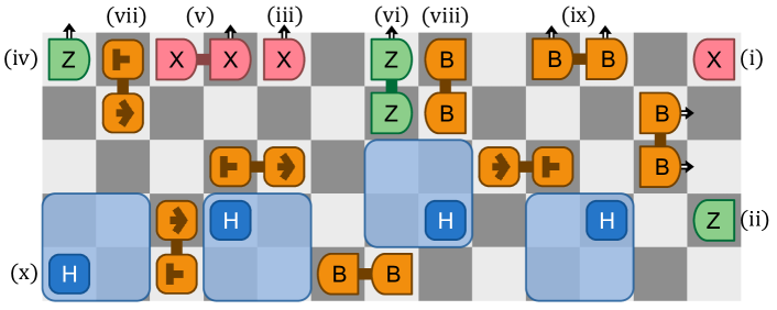
Figure 1: Logical qubits (light and dark gray patches) encoded in the surface code form a 2D grid. The elementary operations can be applied on any lattice translations of those shown. Their times in units of surface code logical time steps are as follows. $\mathit{0}$ logical time steps: Single-qubit preparation in the $X$ basis (i), and the $Z$ basis (ii). Destructive single-qubit measurement, which moves the patch outside of the code space, in the $X$ basis (iii), and the $Z$ basis (iv) take $0$ steps. $\mathit{1}$ logical time step: Two-qubit measurement of $XX$ (v) and $ZZ$ (vi). A move of a logical qubit from one patch to an unused patch (vii). Two-qubit preparation (viii) and destructive measurement (ix) in the Bell basis. $\mathit{3}$ logical time steps: A Hadamard gate, which uses three ancilla patches (x). See Appendix A for further details.

In this work, we seek to minimize the resources required to fault-tolerantly implement a quantum algorithm using the surface code architecture, which we will refer to as the surface code compilation problem. For concreteness, we will assume that the input quantum algorithm is expressed as a quantum circuit composed of preparations and destructive measurements of individual qubits in the $Z$ or $X$ basis, controlled-not (cnot), Pauli-$X$, -$Y$, and -$Z$, Hadamard ($H$), Phase ($S$) and $T$ gates. Our results can be easily generalized to broader classes of input quantum circuits. The output is the quantum algorithm executed using the elementary logical surface code operations shown in Figure 1. Ultimately, we would like to minimize the physical space-time cost, which is the product of the number of physical qubits and the time required to run an algorithm. To avoid implementation details, we instead minimize the more abstract logical space-time cost, which is the number of logical qubits (the circuit width) multiplied by the number of logical time steps (the circuit depth) of the algorithm expressed in elementary surface code operations. The logical and physical space-time costs are expected to be 1-to-1 and monotonically related (see Appendix B), such that minimizing the former should minimize the latter.

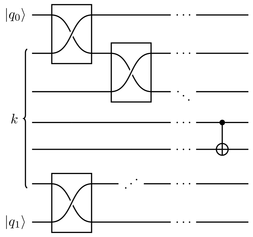
(a) With swap operations

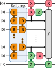
(b) With Bell pair

Figure 2: Application of a cnot$(q_{0},q_{1})$ on qubits at distance $k+1$ using surface code operations in two ways. (a) Using a swap-based approach requires $\Omega(n)$ depth using operations from Figure 1, while (b) generating and consuming a Bell pair [LO17] can be implemented in constant depth. The classical function $f$ computes Pauli corrections on the output qubits.

A well-established approach to implement surface code compilation is known as sequential Pauli-based computation [Lit19], where non-Clifford operations are implemented by injection using Pauli measurements, and Clifford operations are conjugated through the circuit until the end. The circuit that is run in this approach then consists of a sequence of high-weight Pauli measurements which can have overlapping support leading them to be measured one after the other. For large input circuits this can be problematic because highly parallel input circuits can become serialized with prohibitive runtimes.

A major challenge to solve the surface code compilation problem is that quantum algorithms typically involve operations between logical qubits that are far apart when laid out in a 2D grid. One approach to deal with a long-range gate is to swap logical qubits around until the pair of interacting qubits are next to one-another [CSU19]. However, this can result in a deep circuit, see Figure 2(a). A more efficient approach is to create long-range entanglement by producing Bell pairs, which for example can be used to implement a long-range cnot with a constant-depth circuit [Bri+98, LO17, Jav+17] (see Figure 2(b)). Both of these approaches can be implemented with the elementary operations of the surface code.

Moreover, algorithms typically consist of many long-range operations that can ideally be performed in parallel. For swap-based approaches, this can be done by considering a permutation of the logical qubits which is implemented by a sequence of swaps [Lao+18, Mur+19, ZW19]. Finding these swap circuits reduces to a routing problem on graphs [CSU19, SHT19]. There are efficient algorithms that solve this problem for certain families of graphs [ACG94, CSU19], but finding a minimal depth solution is NP-hard in general [BR17]. Alternatively, linear network coding can be used to prepare many long-range pairs in constant depth [LOW10, Kob+09, Kob+11, SLI12, HPE19, BH20], and then these Bell pairs can be used to implement operations on pairs of distant qubits. But a major barrier for using linear network coding is the lack of known efficient algorithms to find linear network codes.

In this paper, we provide a solution to the surface code compilation problem which generalizes the use of entanglement for long-range cnots discussed above to the implementation of many long-range operations in parallel. In particular, we propose the Edge-Disjoint Paths Compilation (EDPC) algorithm, which is a computationally efficient classical algorithm tailored to the elementary operations of the surface code architecture. We find evidence that our EDPC algorithm significantly outperforms other approaches by performing a detailed cost analysis for the execution of a set of quantum circuits benchmarks.

EDPC reduces the problem of executing quantum circuits to problems in graph theory. Logical qubits correspond to graph vertices, and there is an edge between qubits if elementary surface code operations can be applied between them. We show how to perform multiple long-range cnots in constant depth along a set of edge-disjoint paths (EDP) in the graph. In other words, long-range cnots can be performed simultaneously, in one round, if their controls and targets are connected by edge-disjoint paths. This leads to the well-studied problem of finding maximum EDP sets [Kle96]. The ability to perform long-range cnots along with the elementary operations allows compilation of Clifford operations. We also give a construction for EDP sets that are asymptotically optimal in the depth of worst-case sets of independent cnots.

	Input circuit (compiled depth)
Algorithm	1 cnot	$n/2$ parallel cnots	$k$ parallel rotations
Sequential Pauli	0	0	$\Theta(k)$
swap	$\Theta(\sqrt{n})$	$\Theta(\sqrt{n})$	$\Theta(\sqrt{n})$
Network coding	$\Theta(1)$	$\Omega(\sqrt{n})$	$\Omega(\sqrt{k})$
EDPC	$\bm{{\Theta(1)}}$	$\bm{{\Theta(\sqrt{n})}}$	$\bm{{\Theta(\sqrt{k})}}$

Table 1: A comparison in the depth of surface code compilation algorithms (that use $\Theta(n)$ space) for various input circuits of width $n$. We compare the worst-case performance for a single long-range cnot gate, for cnot circuits with $n/2$ parallel cnot gates, and for $k$ rotations, with $k\in\mathbb{N}$, that need to be performed at the boundary.

The final operations that complete our gate set for universal quantum computation with the surface code are $T$ gates. The $T$ gates are not natural operations on the surface code, but can be implemented fault-tolerantly by consuming specialized resource states, called magic states. Magic states can be produced using a highly-optimized process called magic state distillation, which we assume occurs independently of the computation on our code. We assume that logical magic states are available in a specified region of the grid. EDPC reduces magic state delivery to simple Max Flow instances that have known efficient algorithm [FF56]. We compare the depth of input circuits compiled using surface code compilation algorithms in the literature and EDPC in Table 1.

The outline of the paper is as follows. In Section 2, we construct key higher-level components from the basic surface code operations in Figure 1 including simple long-range operations. These long-range operations allow us to perform many parallel cnot operations given vertex-disjoint and edge-disjoint paths that connect the data qubits in Section 3. Because of its importance to the algorithms, there we also compare the state of the art graph algorithms for finding vertex-disjoint or edge-disjoint sets of paths and analyze their relation to our algorithms. We complete our gate set by giving an algorithm for efficient remote rotations using magic states at the boundary in Section 4. Putting parallel long-range cnot and remote rotations together, we construct our circuit compilation algorithm, EDPC, in Section 5. Finally, we compare the performance of EDPC to prior surface code compilation work in Section 6, note its connections to network coding, and give numerical results comparing the space-time performance with a swap-based compilation algorithm.

2 Key circuit components from surface code operations

Recall that our goal in this work is to develop an efficient classical compilation algorithm which re-expresses a quantum algorithm into one that uses the elementary operations of the surface code with a low logical space-time cost. In Appendix A we give an overview of the surface code and justify the resource costs of the elementary operations shown in Figure 1. The initial quantum algorithm is assumed to be expressed as a circuit diagram involving preparations and measurements of individual qubits in the computational basis, controlled-not (cnot), Pauli-$X$, -$Y$, and -$Z$, Hadamard ($H$), Phase ($S$) and $T$ gates. In this section we build and calculate the cost of some key circuit components from the elementary surface code operations in Figure 1. The contents of this section are reproductions or straightforward extensions of previously-known circuits.

2.1 Single-qubit operations

Some of the operations of the input circuit can be implemented directly with elementary surface code operations, namely the preparation and measurement of individual qubits in the measurement basis, and the Hadamard gate (provided three neighboring ancillary patches are available as ancillas, see Figure 1). Pauli operations do not need to be implemented at all since they can be commuted through Clifford gates and arbitrary Pauli gates [Kni05] and can therefore be tracked classically and merged with the final measurements. For this reason, while we occasionally explicitly provide the Pauli corrections where instructive, we often show equivalence of two circuits only up to Pauli corrections. The remaining single-qubit operations in the input circuit, namely the $S$ and $T$ gates, can be implemented using magic states and is addressed in Section 4.

2.2 Local cnot and swap gates

An important circuit component is the cnot gate, which can be implemented as shown in Figure 3(a) [ZBL08]. The qubits involved in this example are stored in adjacent patches, i.e., it is local. Another useful operation is a swap of a pair of qubits stored in nearby patches. The surface code’s move operation shown in Figure 1 gives a straightforward way to implement this as shown in Figure 3(b). With these implementations, the cnot requires one ancilla patch, while swap requires two. Both are depth $2$.

(a) cnot gate

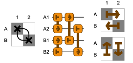
(b) swap gate

Figure 3: A cnot gate can be implemented in depth $2$ using $ZZ$ and $XX$ joint measurements with a $|+\rangle$ ancilla state, followed by classically controlled Pauli corrections. The swap gate can be implemented using four move operations and two ancillas in depth $2$.

2.3 Long-range cnot using swap gates

Figure 4: A non-local cnot can be implemented using swaps which takes depth $2\lceil\frac{k-1}{2}\rceil$ using a zig-zag of ancilla patches along the path $P$ of length $k$. The figure shows the case when $k$ is odd and swaps depth is $2(k-1)$. The patches on the path can store other logical information, which will simply be moved during the swap gates. The patches adjacent to the path are ancillas which are used to implemented the swap gates.

Typical input circuits for surface code compilation will involve cnot operations on pairs of qubits that are far apart after layout. A very intuitive approach to apply a long-range cnot$(q_{1},q_{2})$ gate is shown in Figure 4. This involves making use of swap gates to first move the qubits $q_{1}$ and $q_{2}$ so that they are near one another, and then use the local cnot gate in Figure 3(a). Let the path $P=v_{1}v_{2}\dots v_{k}$, for $k\in\mathbb{N}$, where $v_{1}=q_{1}$ and $v_{k}=q_{2}$. As each swap has depth $2$, we get a circuit of depth $2\lceil\frac{k-1}{2}\rceil$ since we can perform swaps on either end simultaneously. Afterwards, the two qubits are adjacent and we simply perform a cnot in depth $2$.

A lower bound on the depth it takes to perform a long-range cnot gate using swaps is proportional to the length of the shortest $q_{1}$-$q_{2}$ path. To move a qubit $k$ patches using swaps takes depth exactly $2k$. Therefore, to move control and target to the middle of the shortest path connecting them, it must take time proportional to at least half the length of the path.

2.4 Long-range cnot using a Bell pair

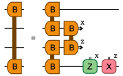
(a) Preparing a longer-range Bell pair

(b) cnot by consuming a Bell pair

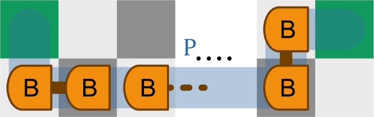
(c) Preparing and consuming a Bell pair for long-range cnot I

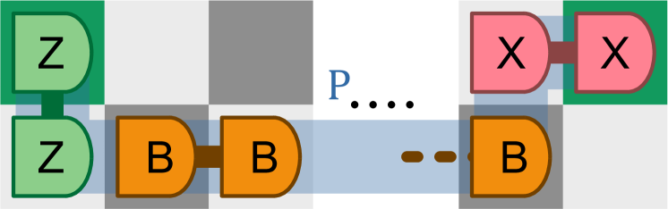
(d) Preparing and consuming a Bell pair for long-range cnot II

Figure 5: A long-range cnot can be implemented in depth $2$ by first preparing a Bell pair. (a) Joining Bell pairs with Bell measurements. This can be iterated to form a long-range Bell pair along any path of ancillas in depth $2$. (b) A Bell pair can be used to apply a cnot. (c,d) The first and second steps of a depth-2 circuit that implements a cnot between a pair of patches at the end of a path of ancilla patches by preparing and consuming a Bell pair.

A circuit component that we make extensive use of in this paper is the long-range cnot using a Bell pair [LO17]. This allows us to apply cnots in depth $2$ between any pair of qubits (provided there is a path of ancilla qubits which connects them).

To understand the construction, we first show in Figure 5(a) how to prepare a longer-range Bell pair from two Bell pairs. By iterating this construction one can form a circuit to prepare a long-range Bell pair at the ends of any path of adjacent ancilla patches in depth $2$. Next, we show in Figure 5(b) how to implement a cnot operation between qubits stored in patches neighboring a pair of patches storing a Bell pair. Putting these together, using a path of ancilla patches between a pair of qubits, a long-range cnot can be implemented in depth $2$ in a two-step circuit shown in Figure 5(c) and Figure 5(d) respectively. This approach can be used to implement the cnot in depth $2$ circuit using any path from the control to the target qubit which starts with a vertical edge and ends with a horizontal edge. There is also flexibility in the precise arrangement of the Bell pairs and Bell measurements along the path using the circuits in Appendix C.

Note that here we have focused on implementing a long-range cnot by constructing and consuming a Bell pair. However a similar strategy (of first preparing a long-range Bell pair in the patches at the ends of a path of ancillas) can be used to implement other long-range operations such as teleportation.

3 Parallel long-range cnots using Bell pairs

Here, we generalize the use of Bell pairs from the setting of compiling an individual non-local cnot gate into surface code operations to the setting in which a set of parallel non-local cnot gates are compiled. In Figure 1 and the circuit components in Section 2, ancilla qubits are used to perform some operations on data qubits. To consider the compilation on large sets of qubits, we must specify the location of data and ancilla qubits: here we assume a 1 data to 3 ancilla qubit ratio, as illustrated in Figure 7.

In Section 3.1 we discuss some relevant background on sets of vertex-disjoint paths (VDP) and sets of edge-disjoint paths (EDP) in graphs. Then in Section 3.2 we define the VDP subroutine and the EDP subroutine that apply parallel cnot gates at the ends of a particular type of VDP or EDP set. In Section 3.3, we show how to use the EDP subroutine to compile more general cnot circuits and prove bounds on the performance of this approach.

3.1 Vertex-disjoint paths (VDP) and edge-disjoint paths (EDP)

In Section 2.4 we saw that a long-range cnot could be implemented with the use of a Bell pair produced with a path of ancilla qubits connecting the control and target of the cnot. A barrier to implement multiple cnots simultaneously can arise when an ancilla resides in the paths associated with multiple different cnots. This motivates us to review some relevant theoretical background concerning sets of paths on graphs.

Given a graph $G$, a set of paths $\mathcal{P}$ is said to be a vertex-disjoint-path (VDP) set if no pair of paths in $\mathcal{P}$ share a vertex, and an edge-disjoint-path (EDP) set if no pair of paths in $\mathcal{P}$ share an edge. Note that a set of vertex-disjoint paths is also edge-disjoint. Further consider a set of terminal pairs $\mathcal{T}=\{(s_{1},t_{1}),\dots,(s_{k},t_{k})\}$ for terminals $s_{i},t_{i}\in V(G)$, the vertices of $G$, and $i\in[k]$. We then say that a set of paths $\mathcal{P}$ is a VDP set for $\mathcal{T}$ (respectively an EDP set for $\mathcal{T}$) if $\mathcal{P}$ is a VDP set (respectively an EDP set), and each path in $\mathcal{P}$ connects a distinct pair in $\mathcal{T}$. These path sets do not necessarily connect all pairs in $\mathcal{T}$. In what follows, we pay special attention to the square grid graph (see Figure 9(a)). The grid graph is relevant for qubits in the surface code as shown in Figure 1, where the vertices correspond to code patches and edge connect vertices associated with adjacent patchs.

The problems of finding a maximum (cardinality) VDP set for $\mathcal{T}$ or a maximum EDP set for $\mathcal{T}$ have been well-studied and there are known efficient algorithms capable of finding approximate solutions to each. Unfortunately, on grids it is particularly hard to approximate the maximum VDP set. In particular, for $N\coloneqq\lvert V(G)\rvert$ there exist terminal sets for which no efficient algorithm can find an approximate solution to within a $2^{O(\log^{1-\epsilon}N)}$ factor of the maximum set size for any $\epsilon>0$, unless $\mathrm{NP}\subseteq\mathrm{RTIME}(N^{\operatorname{poly}\log N})$ [CKN18]. However, efficient algorithms are available if one is willing to accept a looser approximation to the optimal solution. For example, a simple greedy algorithm is an $O(\sqrt{N})$-approximation algorithm for finding the maximum VDP set [KS04, KT06], i.e., it produces a VDP set to within an $O(\sqrt{N})$ multiplicative factor of the optimal solution for any graph, not just the grid. For grids, the best efficient algorithm that is known is an $\tilde{O}(N^{1/4})$-approximation algorithm [CK15], where $\tilde{O}(\cdot)$ hides logarithmic factors of $O(\cdot)$.

The situation is better for approximation algorithms of the maximum EDP set: There is a $\Theta(\sqrt{N})$-approximation algorithm [CKS06] for any graph, and on grids [AR95] showed an $O(\log N)$-approximation algorithm that was later improved to an $O(1)$-approximation algorithm [KT95, Kle96]. In practice, these algorithms can be technical to implement and can have large constant prefactors in their solutions that can be prohibitive for the instance sizes that we consider. A simple greedy algorithm forms a $O(\sqrt{N})$-approximation algorithm [KS04] for finding a maximum EDP set on the two-dimensional grid and does not suffer from the constant prefactors of the asymptotically superior alternatives. The dominant runtime complexity of this greedy algorithm is mainly in finding shortest paths for each terminal pair, giving a $O(\lvert\mathcal{T}\rvert N\log N)$, runtime upper bound by Dijkstra’s algorithm.

It is informative to consider the comparative size of the maximum EDP and VDP sets for the same terminal set $\mathcal{T}$. Since any VDP set is also an EDP set, the size of the maximum VDP set for $\mathcal{T}$ cannot be larger than the maximum EDP set for $\mathcal{T}$. Moreover, one can construct some cases of $\mathcal{T}$ on the grid [Kle96] in which the maximum EDP set is a factor $\sqrt{N}$ larger than the maximum VDP set [Kle96]. For example, consider the set of terminal pairs $\mathcal{T}=\{((i,1),(L,i))\mid i\in[L]\}$ of an $L\times L$ grid graph, where vertex $(i,j)$ denotes the vertex in row $i$ and column $j$. All terminals can be connected by edge-disjoint paths but the maximum VDP set is of size one.

In Section 3.2, we show that both VDP and EDP sets for $\mathcal{T}$ can be used to form constant-depth compilation subroutines for disjoint cnot circuits. Ultimately, as will become clear in Section 3.2, each path in the EDP or VDP sets for $\mathcal{T}$ allows us to implement one more cnot gate in parallel by a compilation subroutine. In this work, we focus on EDPs rather than VDPs for two main reasons. Firstly, as mentioned above, better approximation algorithms exist for finding maximum EDP sets than for finding maximum VDP sets on the grid. Although, in practice, we make use of the greedy $O(\sqrt{N})$-approximation algorithm for finding maximum EDP sets in this work. Secondly, as was also mentioned above, the maximum EDP set is at least as large as the maximum VDP set.

An important open problem that could ultimately influence the performance of the surface code compilation algorithm we present in this work is whether an alternative approximation algorithm for finding maximum EDP sets can be used that performs better in practical instances.

3.2 Long-range cnot subroutines using VDP and EDP

Here we present one of our main technical contributions, namely a description of how to implement a set of long-range cnots at the end of VDP and EDP sets using surface code operations. This is central to our overall surface code compilation algorithm presented in Section 5.

Consider the $L\times L$ square grid graph $G$ (see Figure 9(a)), which consists of vertices $V(G)=[L]\times[L]$, for $[L]\coloneqq\{1,\dots,L\}$ and undirected edges

$$E(G)=\{((i,j),(i,j+1))\mid i\in[L],j\in[L-1]\}\\ \cup\{((i,j),(i+1,j))\mid i\in[L-1],j\in[L]\}.$$ (1)

Here, vertices correspond to qubits stored in surface code patches, and edges connect qubits on adjacent patches (see Figure 1). We color the vertices of $G$ with three colors: black, grey, and white (see Figure 7). All vertices with both even row and even column index are colored black and correspond to data qubits (where data qubits correspond to qubits in the input circuit). The vertices (corresponding to ancilla qubits) with both odd row and odd column index are colored white, and all remaining vertices are colored grey. This gives us a $1:3$ data qubit to ancilla qubit ratio. We set $n$ to equal the number of black vertices, i.e., the number of data qubits.

Due to the designation of some vertices as data qubits and others as ancilla vertices in our layout, and due to the asymmetry of two-qubit operations along horizontal and vertical edges in Figure 1, we add some restrictions to the paths we consider. We define an operator path to be a path $P=v_{1}v_{2}\dots v_{k}$, for $k\in\mathbb{N}$, such that $v_{1}$ and $v_{k}$ correspond to data qubits and its interior $v_{2}\dots v_{k-1}$ are all ancilla qubits. Moreover, $v_{1}$ to $v_{2}$ must be a vertical edge, and $v_{k-1}$ to $v_{k}$ must be a horizontal edge. Then an operator VDP (resp. EDP) set is a set of vertex-disjoint (resp. edge-disjoint) operator paths. In addition, we require that the ends of the paths in the operator EDP set do not overlap. With the coloring assignments of the grid graph $G$, it is easy to see that the first and last vertex of an operator path are colored black. In what follows, we show how we can implement cnots between the data qubits at the ends of the paths in an operator VDP (EDP) set in constant depth.

First consider an operator VDP set $\mathcal{P}$. It is straightforward to see that we can simultaneously apply long-range cnots along each $P\in\mathcal{P}$ as in Figure 5 in depth 2. We call this the vertex-disjoint paths subroutine (VDP subroutine).

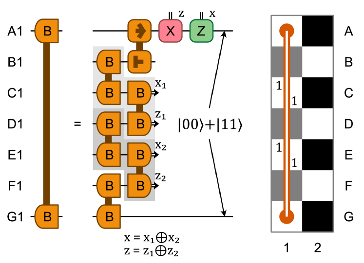
(a) Long-range Bell pair preparation

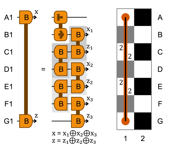
(b) Long-range Bell measurement

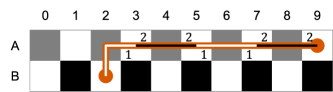
(c) Two-stage Bell preparation using segments

Figure 6: (6(a)) For segments marked in white, we use long-range Bell pair preparation in depth $2$. (6(b)) For segments marked in black, we then use long-range Bell pair measurement in depth $2$. (6(c)) The Bell measurements in stage 2 stitch together the Bell pairs made in phase 1, resulting in a Bell pair in the qubits at the ends of the full path.

Now consider an operator EDP set $\mathcal{P}$. An EDP set can have intersecting paths, and the ancilla qubits at intersections appear in multiple paths, preventing us from simultaneously producing Bell pairs at their ends. We circumvent this by producing Bell pairs across a path in two stages by splitting the path into segments; see Figure 6. We will show that $\mathcal{P}$ can be fragmented into two VDP sets $\mathcal{P}_{1}$ and $\mathcal{P}_{2}$ that, together, form $\mathcal{P}$. More precisely, each path $P\in\mathcal{P}$ can be built by composing paths contained in $\mathcal{P}_{1}$ and $\mathcal{P}_{2}$ such that each path in either $\mathcal{P}_{1}$ or $\mathcal{P}_{2}$ appears in precisely one path in $\mathcal{P}$. We say that the paths in $\mathcal{P}_{1}$ and $\mathcal{P}_{2}$ are segments of paths in $\mathcal{P}$. This forms the basis of the edge-disjoint paths subroutine (EDP subroutine), which is presented in Algorithm 3.1 and illustrated with an example in Figure 7.

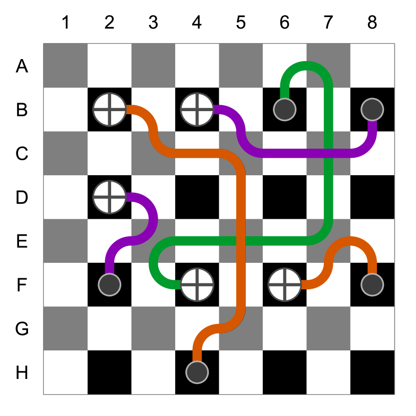
(a) cnot gates and edge-disjoint paths.

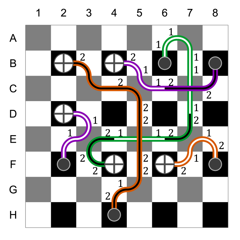
(b) Execution stages assignment

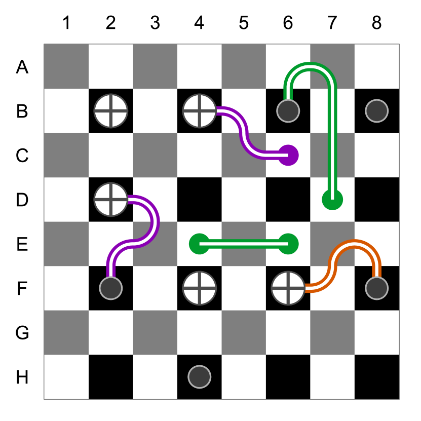
(c) First stage. State preparation.

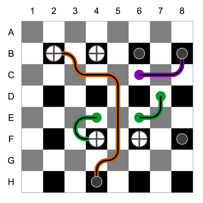
(d) Second stage. Measurements.

Figure 7: The EDP subroutine implements a set of parallel cnots connected by an operator EDP set. We assume a qubit ratio of 1 to 3 of data (black) to ancilla (gray and white). (7(a)) The input to the EDP subroutine is a set of cnots and an associated EDP set. (7(b)) We fragment the EDP set into two VDP sets consisting of segments of the original paths, and implement the compiled circuit over two depth-2 stages, one for each of these sets. (7(c)) During the first stage we prepare a Bell pair between the ends of the segments in the first VDP set. (7(d)) During the second stage we perform joint Bell measurements between the ends of segments in the second VDP set, producing long-range Bell pairs on ancillas adjacent to the control and target of each cnot. Then, long-range cnots can easily be applied by using the long-range Bell pairs (Section 2.4). See Figures 6 and 8 for further details of the long-range operations used here.

Input : An operator EDP set $\mathcal{P}$

$\mathcal{P}_{1},\mathcal{P}_{2}\leftarrow$ fragment $\mathcal{P}$ in two VDP sets of segments;

  // Theorem 3.2

1 for segment $P\in\mathcal{P}_{1}$ :

2      if $P$ connects two data qubits then

3            execute long-range cnot along $P$;

4            

5      else

6            execute phase 1 operation along $P$ (Figure 6(a), or 8(b), or 8(c));

7            

8for segment $P\in\mathcal{P}_{2}$ :

9      if $P$ connects two data qubits then

10            execute long-range cnot along $P$;

11            

12      else

13            execute phase 2 operation along $P$ (Figure 6(b), or 8(d), or 8(e));

14            

Algorithm 3.1 EDP subroutine: to apply cnots to the data qubits at the endpoints of a set of edge-disjoint paths $\mathcal{P}$, where the interior of each path is supported on ancilla qubits. The depth is at most 4.

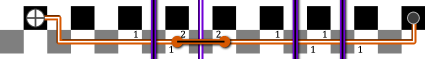
(a) Long-range cnot in two stages

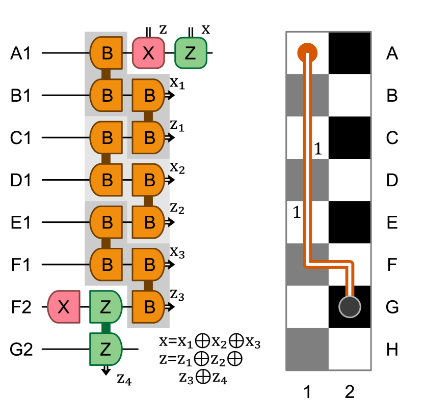
(b) Long-range X prep. with ZZ meas.

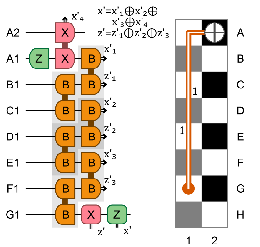
(c) Long-range Z prep. with XX meas.

(d) Long-range teleport with ZZ meas.

(e) Long-range teleport with XX meas.

Figure 8: Detailed implementation of the steps in Figure 7. For each segment that is scheduled in phase 1, we use (8(b)) and (8(c)); and for each supbath that is scheduled in phase 2, we use (8(d)) and (8(e)). In (8(d)) variables $x_{0}$ and $z_{0}$ equal to the total parity of all long-range Bell measurements applied during stage 2 on the cnot path. Each of these operations takes depth $2$. (8(d)) and (8(e)) share the variables $a$ and $c$.

We show the following Lemma, which restricts the adjacency of crossing vertices. As will become clear later, the adjacent crossing vertices impose systems of constraints on fragmenting $\mathcal{P}$, and their restricted adjacency of any operator EDP set ensures a fragmentation into two VDP sets always exists.

Lemma 3.1.

Given an operator EDP set $\mathcal{P}$, a crossing vertex is a vertex contained in more than one path in $\mathcal{P}$. Let the set of crossing vertices be $V_{c}$, then the induced subgraph $G[V_{c}]$ contains only three kinds of connected components:

1. Isolated vertices.

2. A horizontal path, where each vertex $(i,j)$ in the connected component can only be adjacent to $(i-1,j)$ and $(i+1,j)$.

3. A vertical path, where each vertex $(i,j)$ in the connected component can only be adjacent to $(i,j-1)$ and $(i,j+1)$.

Proof.

We consider all possible colors of a vertex $(i,j)$ in a connected component of $G[V_{c}]$. Black vertices cannot be crossing vertices by definition of an operator EDP set so cannot be contained in $V_{c}$. It is then easy to see that white vertices in $V_{c}$ satisfy the Lemma.

Therefore, the only relevant case is when $(i,j)$ is a grey vertex. The vertices $(i+1,j)$ and $(i,j+1)$ are white and $(i+1,j+1)$ is black. We show that these white vertices cannot both be crossing vertices. Suppose that they are, then both edges between the white vertices and the black vertex, $((i+1,j),(i+1,j+1))$ and $((i,j+1),(i+1,j+1))$, are in $\mathcal{P}$. This is a contradiction with the fact that the interior of operator EDP paths cannot contain a black vertex so it must be at the end of two paths, but an operator EDP set cannot contain two paths ending at the same vertex. By the same argument applied to the other white neighbors of $(i,j)$ we see that only $(i-1,j)$ and $(i+1,j)$ or $(i,j-1)$ and $(i,j+1)$ can both be crossing vertices, and the claim follows. ∎

We now prove that $\mathcal{P}$ can be fragmented.

Theorem 3.2.

We can fragment an operator EDP set $\mathcal{P}$ to produce vertex-disjoint sets of segments $\mathcal{P}_{1}$ and $\mathcal{P}_{2}$. If $\mathcal{P}$ is vertex-disjoint, then $\mathcal{P}_{1}=\mathcal{P}$ and $\mathcal{P}_{2}=\emptyset$.

Proof.

We assign edges for inclusion in segments in $\mathcal{P}_{1}$ or $\mathcal{P}_{2}$ by an edge labelling $l(e)\colon E(G)\to\{1,2\}$. Given a labelling of all edges $e$ in the paths of $\mathcal{P}$, we can assign edges $l(e)=b$ to segments in $\mathcal{P}_{b}$. Therefore, given a labelling of all edges in paths in $\mathcal{P}$, it is easy to construct $\mathcal{P}_{1}$ and $\mathcal{P}_{2}$. We now label all edge in the paths in $\mathcal{P}$ and prove that their labelling guarantees the vertex-disjointness property of $\mathcal{P}_{1}$ and $\mathcal{P}_{2}$.

We constrain the labeling around every crossing vertex $v$ so that the VDP property is satisfied. Clearly, $v$ is contained in the interior of exactly two paths, $P_{1}$ and $P_{2}$. Let $v$ be contained in edges $e_{1}$ and $e_{1}^{\prime}$ of $P_{1}$, and edges $e_{2}$ and $e_{2}^{\prime}$ of $P_{2}$, then we impose the constraints

$$l(e_{1}) =l(e_{1}^{\prime})$$ (2)

$$l(e_{2}) =l(e_{2}^{\prime})$$ (3)

$$l(e_{1}) \neq l(e_{2})$$ (4)

guaranteeing the vertex-disjointness of segments at $v$ since a segment of $P_{1}$ must span both $e_{1}$ and $e_{1}^{\prime}$, and a segment of $P_{2}$ must span both $e_{2}$ and $e_{2}^{\prime}$ with a different label.

We show there always exists a feasible solution given these constraints. If we consider the graph $G[V_{c}]$ induced by crossing vertices $V_{c}$, then we see that every connected component in $G[V_{c}]$ gives a system of constraints. The adjacency of $G[V_{c}]$, by Lemma 3.1, is such that each system has one degree of freedom, which we decide arbitrarily.

Finally, for every vertex-disjoint path $P\in\mathcal{P}$, assign $l(e)=1$ to all edges $e$ in $P$. All remaining edges can be labeled arbitrarily. ∎

The depth of a cnot circuit produced by the EDP subroutine for an operator EDP set $\mathcal{P}$ is at most 4. If $\mathcal{P}$ happens to be vertex-disjoint, then the depth is 2 since all paths are assigned to phase 1 by Theorem 3.2.

3.3 Compiling parallel cnot circuits with the EDP subroutine

In this section we consider how to compile input parallel cnot circuits using the EDP subroutine. We define the terminal pairs $\mathcal{T}\subseteq V(G)\times V(G)$ to be the pairs of control and target qubits for each cnot gate in the parallel cnot circuit. To use the EDP subroutine, we need to find operator EDP sets $\mathcal{P}_{1},\dots,\mathcal{P}_{k}$ that connect all terminal pairs in $\mathcal{T}$. We will refer to any such set $\{\mathcal{P}_{1},\dots,\mathcal{P}_{k}\}$ as a $\mathcal{T}$-operator set. The depth of the compiled implementation is minimized when the size $k$ of the $\mathcal{T}$-operator set is minimized.

There are reasons to believe that the compilation strategy for parallel cnot-circuits formed by finding a minimal $\mathcal{T}$-operator set and applying the EDP subroutine should produce low-depth output circuits. For sparse input circuits, i.e. those with a small number of cnots, one can expect a small $\mathcal{T}$-operator set to exist, giving a low depth output. On the other hand, we now prove that there are dense cnot circuits for which the EDP subroutine with a minimal size $\mathcal{T}$-operator set produces a compiled circuit with optimal depth (up to a constant multiplicative factor).

Theorem 3.3.

Let a parallel input cnot circuit with corresponding terminal pairs $\mathcal{T}$ be given, and let the $n$ qubits of the input circuit be embedded in a grid among $3n$ ancilla qubits according to the layout in Figure 7. For simplicity, we assume $n$ is both even and the square of an integer. We can find a $\mathcal{T}$-operator set of size at most $2\sqrt{n}-1$ in polynomial time.

Proof.

For each cnot we construct an operator path and argue that all such paths can be grouped into $O(\sqrt{n})$ disjoint EDP sets. For simplicity, in the following, we specify paths by a sequence of key vertices, with each consecutive pair of key vertices connected by the shortest path (which is a horizontal or a vertical line).

We now construct an operator path for each cnot, where the associated control vertex is $v=(v_{x},v_{y})\in V(G)$ and the target vertex is $u=(u_{x},u_{y})\in V(G)$. We can always form an operator path to connect $u$ and $v$ given by the following sequence of five key vertices $v$, $(v_{x},v_{y}-1)$, $(u_{x}-1,v_{y}-1)$, $(u_{x}-1,u_{y})$, $u$. This path consists of one vertical end segment, one horizontal interior segment, one vertical interior segment, and finally a horizontal end segment.

Having assigned a path to each cnot, we now show that any of these operator paths can share an edge with at most $2(\sqrt{n}-1)$ of the other paths. Since the operator paths have distinct endpoints, two different paths cannot share an edge on either of their end segments $v,(v_{x},v_{y}-1)$ and on $(u_{x}-1,u_{y}),u$. Therefore pairs of these operator paths can only share an edge on their interior segments. The horizontal interior segment of the operator path from $v$ to $u$ can share an edge with at most $\sqrt{n}-1$ other paths. To see this, consider an operator path from $v^{\prime}=(v^{\prime}_{x},v^{\prime}_{y})\in V(G)$ to $u^{\prime}=(u^{\prime}_{x},u^{\prime}_{y})\in V(G)$ that shares at least one horizontal edge with the operator path from $v$ to $u$. Explicitly, that means the segment $(v_{x},v_{y}-1)$, $(u_{x}-1,v_{y}-1)$ shares an edge with the segment $(v^{\prime}_{x},v^{\prime}_{y}-1)$, $(u^{\prime}_{x}-1,v^{\prime}_{y}-1)$, which implies that $v_{y}=v^{\prime}_{y}$. Since the terminals are unique, there can only be $\sqrt{n}-1$ other cnots with the control sharing the $v_{y}$ coordinate. An analogous argument applies for vertical segments, such that the operator path from $u$ to $v$ can share an edge with at most $2(\sqrt{n}-1)$ other operator paths.

Let us construct a graph $H$ where each vertex represents an operator path as constructed above. We connect two vertices in $H$ if the associated paths share an edge. Every vertex in $H$ has degree at most $2(\sqrt{n}-1)$, therefore, $H$ is $(2\sqrt{n}-1)$-colorable using the (polynomial time) greedy coloring algorithm. We construct a $\mathcal{T}$-operator set of size $2\sqrt{n}-1$ by grouping the paths associated with each color in a set of edge-disjoint paths. ∎

We now show a general lower bound on compiling parallel cnot circuits to the surface code architecture. Our strategy will be to consider a parallel cnot circuit with control data qubits in an area with small boundary that generates an amount of entanglement across the boundary proportional to the area for a given initial state. However, each elementary surface code operation is local such that only those operations acting at the boundary can increase the entanglement across it. The depth of any implementation of the cnot circuit is then lower bounded by the entanglement that it generates over the boundary size [DBT21, Bap+22].

Theorem 3.4.

Consider a surface code architecture of $n$ data qubits embedded in a grid where all ancilla qubits are in the $|0\rangle$ state. For any positive integer $k\leq n/2$, there exists a parallel cnot circuit of $k$ cnot gates with associated terminal pairs $\mathcal{T}$ that needs depth $\Omega(\sqrt{k})$ to be implemented on the surface code architecture.

Proof.

Consider a cnot circuit with terminal pairs $\mathcal{T}$ with control qubits on data vertices in a square region, $V_{L}$, and target qubits on vertices outside $V_{L}$. We initialize the $2k$ data qubits associated with $\mathcal{T}$ to a product state $|+\rangle^{k}|0\rangle^{k}$, with $|+\rangle$ on control qubits and $|0\rangle$ on target qubits (the remaining data qubits are initialized in an arbitrary product state and ignored). After applying the cnot circuit, we obtain $k$ Bell pairs. Therefore, the (von Neumann) entropy of the reduced state of the data qubits in $V_{L}$ has increased from $0$ to $k$.

Consider a circuit $\mathcal{C}$ of depth $d$ that implements the parallel cnot circuit. Any elementary operation of the surface code acting only within $V_{L}$ or within $\bar{V}_{L}\coloneqq V(G)\setminus V_{L}$ or classical communication (together, LOCC) cannot increase the entropy of the state on $V_{L}$. Moreover, as we show below, each elementary operation that acts both on $V_{L}$ and on $\bar{V}_{L}$ can increase the entropy by at most a constant $4$. We can therefore upper bound the increase in entropy due to $\mathcal{C}$ by $4d$ times the number of vertices adjacent to $V_{L}$, which is proportional to $\sqrt{k}$. To attain the $k$ increase in entropy, we therefore need that $d=\Omega(\sqrt{k})$.

We now bound the increase in entropy of any elementary operations acting on $V_{L}$ and $\bar{V}_{L}$ to at most $4$. All such elementary operations are built from a single $XX$ or a $ZZ$ measurements and single qubit operations Appendix A, which cannot increase the entropy. It is possible to implement $XX$ and $ZZ$ measurements acting on $V_{L}$ and $\bar{V}_{L}$ using two cnots and operations acting only within $V_{L}$ or within $\bar{V}_{L}$. The increase in entropy in $V_{L}$ by a cnot operation is bounded by $2$ [Ben+03, Lemma 1]. Therefore, $XX$ measurements, $ZZ$ measurements, and indeed any elementary operation of the surface code can increase the entropy by at most $4$. ∎

In practice, it can be difficult to find minimal-size $\mathcal{T}$-operator sets. However, when the minimal size $\mathcal{T}$-operator set is $k$, in the following theorem we show that a $\mathcal{T}$-operator set $\{\mathcal{P}_{1},\dots,\mathcal{P}_{l}\}$ with size at most $l=O(k\log\lvert\mathcal{T}\rvert)$ can be found by a greedy algorithm that finds iteratively finds the maximum operator EDP set for remaining terminals in $\mathcal{T}$.

Theorem 3.5.

On the grid of $n$ vertices, the greedy algorithm for finding $\mathcal{T}$-operator sets repeats the following two steps , for $i=1,\dots$, until there are no more terminal pairs to connect:

1. find a maximum operator EDP set $\mathcal{P}_{i}$,

2. remove all terminal pairs in $\mathcal{P}_{i}$ from $\mathcal{T}$.

The set $\{\mathcal{P}_{1},\dots,\mathcal{P}_{k}\}$ is a $\mathcal{T}$-operator set and is an $O(\log\lvert\mathcal{T}\rvert)$-approximation algorithm for finding minimum-size $\mathcal{T}$-operator sets.

Proof.

We base our proof on [AR95]. Assume that the minimum-size $\mathcal{T}$-operator set is $\{\mathcal{Q}_{1},\dots,\mathcal{Q}_{K}\}$ for some size $K$. Then there is an operator EDP set $\mathcal{Q}_{i}$, for $i\in[K]$, such that $\lvert\mathcal{Q}_{i}\rvert\geq\lvert\mathcal{T}\rvert/K$. Therefore, the number of unconnected terminal pairs is reduced by at least a factor $(1-1/K)$ each iteration and it will require at most $O(K\log\lvert\mathcal{T}\rvert)$ iterations to connect all terminal pairs [Joh74]. ∎

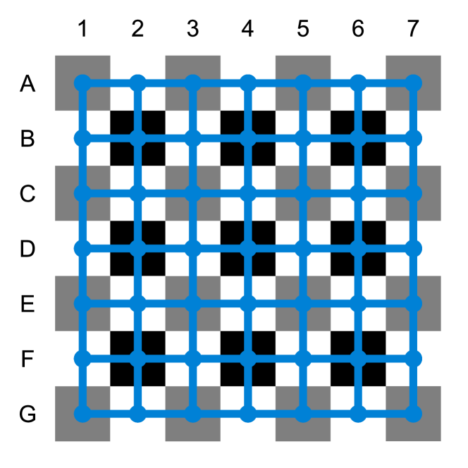
(a) Grid graph

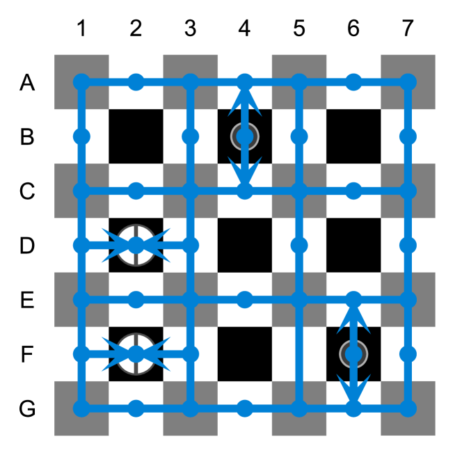
(b) Operator graph

Figure 9: The graphs used in this paper. (9(a)) The grid graph where each surface code patch corresponds to a vertex and is connected to its neighbors. (9(b)) The operator graph for a set of terminal pairs $\mathcal{T}$ that correspond with a parallel cnot circuit. EDP sets for $\mathcal{T}$ on this graph are also operator EDP sets.

To make use of Theorem 3.5 we would ideally like to have an algorithm to find maximum operator EDP sets on the grid, however the efficient algorithms we discussed in Section 3.1 fall short of this in two ways. Firstly they find EDP sets rather than operator EDP sets, and secondly they provide approximate maximum sets rather than maximum sets. Fortunately, we find an equivalence between operator EDP sets on the grid and EDP sets on a graph that we call the $\mathcal{T}$-operator graph (see Figure 9(b)). The $\mathcal{T}$-operator graph is a copy of the grid graph but with all vertices corresponding to control qubits in $\mathcal{T}$ only having vertical outgoing edges, and with all vertices corresponding to target qubits in $\mathcal{T}$ only having horizontal incoming edges, and all remaining vertices corresponding to data qubits are removed. An EDP set for terminal pairs $\mathcal{T}$ on the $\mathcal{T}$-operator graph is an operator EDP set on the grid. It is easy to see that a maximum operator EDP set for $\mathcal{T}$ on the grid is equivalent to a maximum EDP set for $\mathcal{T}$ on the $\mathcal{T}$-operator graph. Using an approximation algorithm for finding the maximum operator EDP set also still gives approximation guarantees for minimizing the $\mathcal{T}$-operator set, as shown in the following Corollary.

Corollary 3.6.

The greedy algorithm for finding minimum $\mathcal{T}$-operator sets, but with a $\kappa$-approximation algorithm for finding maximum operator EDP sets, gives an $O(\kappa\log\lvert\mathcal{T}\rvert)$-approximation algorithm for finding minimum $\mathcal{T}$-operator sets.

Proof.

We modify the proof of Theorem 3.5 such that every iteration we connect a $(1-\kappa/K)$ fraction of unconnected terminal pairs using the $\kappa$-approximation algorithm for finding maximum operator EDP sets. Therefore we obtain a $O(\kappa\log\lvert\mathcal{T}\rvert)$-approximation algorithm for findining minimum $\mathcal{T}$-operator sets. ∎

The equivalence between operator EDP sets on the grid and EDP sets on the $\mathcal{T}$-operator graph motivates us to seek an efficient algorithm to find approximate maximum EDP sets on the $\mathcal{T}$-operator graph as a key part of our EDPC algorithm. The algorithms we discussed in Section 3.1 come close to doing this, but some of them are intended for finding approximate maximum EDP sets on the grid rather than on the $\mathcal{T}$-operator graph and even if they are adapted, the guarantees of the size of the approximate minimum EDP sets they produce may not apply in the case of the $\mathcal{T}$-operator graph. The algorithms described in Refs. [AR95, KT95] for finding approximate maximum EDP sets on the grid do not directly apply to the operator graph. While it seems straightforward to adapt the $O(\log n)$-approximation algorithm [AR95], the algorithms in [AR95, KT95] are complex to implement and have large constant-factor overheads, which can make them impractical on small instance sizes.

Input : $\mathcal{T}$ terminal pairs

1 $\mathcal{Q}_{1}\leftarrow$ the $\mathcal{T}$-operator set given by Theorem 3.3 for $\mathcal{T}$;

2 $\mathcal{Q}_{2}\leftarrow\emptyset$;

3 while $\mathcal{T}\neq\emptyset$ : // Greedy apx. minimum-size $\mathcal{T}$-operator set

4      $\mathcal{P}\leftarrow$ approximately maximize operator EDP set using greedy EDP algorithm [KS04] on operator graph;

5       remove connected terminal pairs in $\mathcal{P}$ from $\mathcal{T}$;

6       $\mathcal{Q}_{2}\leftarrow\mathcal{Q}_{2}\cup\{\mathcal{P}\}$;

7      

8return minimum-size set between $\mathcal{Q}_{1}$ and $Q_{2}$;

Algorithm 3.2 Bounded $\mathcal{T}$-operator set algorithm: An approximation algorithm for minimizing the $\mathcal{T}$-operator set size that combines the theoretical guarantees from Theorem 3.3 with pragmatic performance using the greedy algorithm of Theorem 3.5.

In EDPC, we instead combine the theoretical worst-case bounds of Theorem 3.3 with the pragmatic performance of a greedy approach, which does not have a large constant overhead, in Algorithm 3.2. By Theorem 3.4 this gives us asymptotically tight performance in the worst-case. The runtime of this algorithm is dominated by $O(\lvert\mathcal{T}\rvert)$ iterations of approximately maximizing the operator EDP set in time $O(\lvert\mathcal{T}\rvert n\log n)$. We leave it as an open question to find better approximation algorithms for finding maximum operator EDP sets that give improved performance outside the worst-case and that may also improve the runtime since less iterations over $\mathcal{T}$ are required.

4 Remote rotations with magic states

Thus far we have discussed the surface code compilation of all the input circuit operations listed in Section 1 except for the single-qubit rotation gates $S=Z(\pi/4)$ and $T=Z(\pi/8)$. In this section we design a subroutine for the compilation of parallel rotation circuits. The $S$ and $T$ gates can be implemented by using specially prepared magic states $|S\rangle$ and $|T\rangle$, respectively. Magic states can be prepared using a highly-optimized process known as magic state distillation [Kni04], which distills many faulty magic states that are easy to prepare into fewer robust states. Still, producing both $|S\rangle$ and $|T\rangle$ involves considerable overhead. The $|S\rangle$ state is used to apply the $S$-gate in a ‘catalytic’ fashion, whereby the state $|S\rangle$ is returned afterwards. On the other hand, the state $|T\rangle$ is consumed to apply the $T$-gate. The reason for this distinction is rooted in the fact that the $S$-gate is Clifford but the $T$-gate is non-Clifford.

In this work, we do not address the mechanism by which magic states are produced, but instead assume that these states are provided at specific locations where they can be used to implement gates. More specifically, we assume rotation gates $S$ and $T$ (and also Clifford variations of these such as $X(\pi/8)=T_{x}$ and $X(\pi/4)=S_{x}$) can be applied as a resource on specific ancilla qubits $B\subseteq V(G)$ at the boundary of a large array of logical qubits (Figure 10(a)). This will allow sufficient space outside the boundary where highly-optimized magic state distillation and synthesis circuits can be implemented. Because a large number of magic states are used in the computation, we consider having magic state distillation adjacent to and concurrent with computation we are concerned with in this paper to be a reasonable allocation of resources.

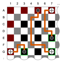
(a) Long-range cnots for diagonal gates

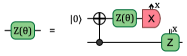
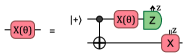
(b) Remote $Z(\theta)$ and $X(\theta)$

Figure 10: We assume the capability of performing $S$ and $T$ gates at the boundary qubits (red) where it is easy for us to supply the requisite $S$ and $T$ magic states. We can then execute $S$ or $T$ gates in the $Z$ or $X$ basis for our circuit by using long range cnots and the circuits in Figure 10(b). For example, to execute $S$ or $T$ on qubits G3, E7 and $HTH$ on G7, we apply long-range cnots between pairs (G3,G1), (E7,A7), (A5,G7) and then execute $S$ or $T$ on G1, A7, HTH on A5. We can continue applying other Clifford gates to qubits G3, E7, and G7 right after performing the long-range cnot, without waiting for the $Z$ correction, since we can propagate the correction through Clifford operations.

We need a technique to apply remote rotations to data qubits which can be far from the boundary making use of the rotations that can be performed at the boundary. We make use of the property that any $Z$ rotation (including $T$ or $S$) has the same action when applied to either qubit in the state $\alpha|00\rangle+\beta|11\rangle$. In particular, these two qubits need not be close to one another, so we can apply $Z$ rotations remotely. A similar notion holds for $X$-rotations (including $T_{x}=HTH$ or $S_{x}=HSH$) and $\alpha|++\rangle+\beta|--\rangle$. Given a qubit $q$ that needs to perform a $Z$ rotation requiring a magic state, we apply a remote $Z$-rotation (Figure 10(b)): by performing a long-range cnot$(q,q^{\prime})$ to a boundary ancilla $q^{\prime}\in B$ prepared in $|0\rangle$. Therefore we can apply the $Z$ rotation remotely and use an $X$ measurement on $q^{\prime}$ to collapse the state back to one logical qubit. Similarly, for a qubit $q$ that needs to perform an $X$ rotation requiring a magic state, we apply a long-range cnot$(q^{\prime},q)$ to an ancilla $q^{\prime}$ prepared in $|+\rangle$ on the boundary, giving

$${\textsc{cnot}}{}|+\rangle(\alpha|+\rangle+\beta|-\rangle)=\alpha|++\rangle+\beta|--\rangle\,.$$ (5)

Therefore we apply the $X$ rotation remotely and collapse the state back by a single-qubit $Z$ measurement of $q^{\prime}$.

The task of compiling a parallel rotation circuit therefore reduces to applying a set of cnot gates from the boundary to the sites of the rotation gates. This can be achieved by finding an appropriate EDP set and running the EDP subroutine of Algorithm 3.1. Compared to the task of finding an EDP set for parallel cnot gates of Section 3, there is one simplifying condition here: Any boundary qubit can be used for each cnot when applying remote rotations. As we explain below, we can find the maximum EDP set for the compilation of remote rotations by solving the following (unit) Max Flow problem [KT06a].

Definition 4.1 (Max Flow).

Given a directed graph $G$ and source and sink vertices $s,t\in V$, we wish to find a flow for all edges of $G$, $f(e)\colon E(G)\to\mathbb{R}$, that is skew symmetric, $f((u,v))=-f((v,u))$, and, for $v\in V(G)\setminus\{s,t\}$, must respect the constraints

$$f(e) \leq 1$$ (6)

$$\text{and}\sum_{u:(v,u)\in E(G)}f((v,u)) =0$$ (7)

such that the outgoing source flow $\lvert f\rvert\coloneqq\sum_{u:(s,u)\in E(G)}f((s,u))$ is maximized.

To understand why this yields a maximum EDP, we first point out that a solution for which $f$ has binary values provides an EDP set by building paths from those edges $e$ for which $f(e)=1$. Moreover, this EDP set must be maximum, because a larger EDP set would imply a larger flow than $f$, which is the maximum flow by definition. Indeed the Ford-Fulkerson algorithm [FF56] solves Max Flow in runtime bounded by $O(\lvert E(G)\rvert\lvert f\rvert)$ and finds flow values $f(e)\in\{0,1\}$ on all $e\in E(G)$ because of the unit capacity constraints, $f(e)\leq 1$. Therefore, $f$ corresponds to a maximum EDP set [KT06a, Section 7.6].

Input : Connectivity graph $G$ with vertices corresponding to boundary qubits $B\subseteq V(G)$ and a set of parallel rotations $\mathcal{G}_{m}$;

1 function max_rotations($\mathcal{G}_{m}$):

2      $W\leftarrow$ vertices associated with qubits in $\mathcal{G}_{m}$;

3       create virtual vertices $s$ and $t$;

4       $G^{\prime}=(V(G)\cup\{s,t\},E(G)\cup\{(s,s^{\prime})\mid s^{\prime}\in W\}\cup\{(t^{\prime},t)\mid t^{\prime}\in B\})$;

5       $f\leftarrow$ solve Max Flow on $G^{\prime}$ using the Ford-Fulkerson algorithm;

6       $\mathcal{P}\leftarrow$ construct edge-disjoint set of $s$–$t$ paths from $f$;

7       return $\mathcal{P}$ with $s$ and $t$ removed from each $P\in\mathcal{P}$;

8      

9while $\mathcal{G}_{m}$ is not empty :

10      $\mathcal{P}\leftarrow$ max_rotations($\mathcal{G}_{m}$);

11       execute remote rotations at boundary with EDP subroutine given $\mathcal{P}$;

12       remove executed rotations from $\mathcal{G}_{m}$;

13      

Algorithm 4.1 Remote rotation subroutine: executes parallel single qubit rotations that require magic states at the boundary by a Max Flow reduction. Using the EDP subroutine (Algorithm 3.1), we can perform remote rotations (Figure 10) on each set of qubits connected to the boundary by $\mathcal{P}$ in depth 4.

The remote rotation subroutine (Algorithm 4.1) executes a set of parallel single-qubit rotations. Each iteration can be performed in depth 4 using the EDP subroutine. On the surface code architecture, we can give strong guarantees on the number of iterations required to execute a set of parallel rotations by the Max Flow to min-cut equivalence.

Theorem 4.2.

The remote rotation subroutine executes all rotations in $\mathcal{G}_{m}$ in depth $O(\sqrt{\lvert\mathcal{G}_{m}\rvert})$.

Proof.

The function max_rotations($\mathcal{G}_{m}$) that is a part of the remote rotation subroutine finds a maximum flow connecting the data qubits performing rotations to the boundary where every additional unit of flow is one more rotation executed. This maximum flow is equal to the minimum edge-cut separating the data qubits from the boundary [FF56]. The boundary of a rectangle containing $\lvert\mathcal{G}_{m}\rvert$ vertices on the grid is of size $\Omega(\sqrt{\lvert\mathcal{G}_{m}\rvert})$, giving a minimum cut size of $\Omega(\sqrt{\lvert\mathcal{G}_{m}\rvert})$. Thus, at most $O(\sqrt{\lvert\mathcal{G}_{m}\rvert})$ iterations of the while loop in the remote rotation subroutine are necessary to implement all remote rotations, as claimed. ∎

We bound the runtime of the remote remote rotation subroutine by $O(n^{2}\sqrt{\lvert\mathcal{G}_{m}\rvert})$ as follows: At most $O(\sqrt{\lvert\mathcal{G}_{m}\rvert})$ iteration of the while loop are necessary (see proof of Theorem 4.2). Each iteration, the call to max_rotations($\mathcal{G}_{m}$) is dominated by solving a Max Flow instance using the Ford-Fulkerson algorithm [FF56], which has a runtime bounded by $O(n^{2})$.

One could consider a number of generalizations and variations of this compilation subroutine for parallel rotation circuits. For instance, when the number of rotation gates is small, it may be useful to find VDP sets rather than EDP sets so that the VDP subroutine rather than the EDP subroutine can be applied. There is a different reduction to Max Flow in this case which can be obtained by replacing each vertex with two vertices, one with incoming edge and one with outgoing edges, connected by a directed edge with capacity 1. This guarantees only one flow can pass through every vertex.

Although we do not consider other single-qubit rotations in our input circuit for compilation, it is worth noting that any single-qubit rotation gate $Z(\theta)$ can be approximately synthesized to arbitrary precision [RS16] using $|S\rangle$ and $|T\rangle$ states along with the surface code operations shown in Figure 1. The approach used to apply $S$ and $T$ gates shown in Figure 10(a) can also be used to apply any rotation $Z(\theta)$ within the grid of surface codes by synthesizing the rotation at the boundary. However, if one considers more general rotations in the input circuit, the time needed for synthesis at the boundary will need to be accounted for and accommodated by other aspects of the overall surface code compilation algorithm. Another extension that can be considered is if multi-qubit diagonal gates are allowed in the input circuit. We show how $X$ and $Z$ rotations generalize to multi-qubit diagonal gates in Appendix D, although we do not use this in our surface code compilation algorithm.

5 EDPC surface code compilation algorithm

In this section we construct the EDPC algorithm for compiling universal input circuits into surface code operations by combining subroutines Algorithm 3.1 and Algorithm 4.1 for compiling long-range cnots and $Z/X$ rotations respectively. First we provide a more formal definition of surface code compilation:

Definition 5.1 (Surface code compilation).

Consider an input quantum circuit of operations $\mathcal{C}=g_{1}g_{2}\dots g_{\ell}$, which is a list of length $\ell$ of operations $g_{i}$ for $i\in[\ell]$, consisting of: state preparation in $X$ or $Z$ basis; the single-qubit operators $X$, $Y$, $Z$, $H$, $S$, $T$, $S_{x}=HSH$, $T_{x}=HTH$; cnot operations; and $X,Z$-measurements. Then a surface code compilation produces an equivalent output circuit $\mathcal{O}$ in terms of surface code operations (Figure 1) on a grid of surface codes with $S$, $T$, $S_{x}$, and $T_{x}$ rotations applied only at the grid’s boundary.

Input : Circuit $\mathcal{C}$ with Paulis commuted to the end and merged with measurement

1

2while available operations in $\mathcal{C}$ :

3      execute all available state preparation, measurement, and Hadamard;

4      

5      run remote rotation subroutine on available rotations;

6       $\mathcal{T}\leftarrow$ terminal pairs associated with available cnots;

7       $\mathcal{Q}\leftarrow$ run bounded $\mathcal{T}$-operator set Algorithm 3.2 on $\mathcal{T}$;

8       for $\mathcal{P}\in\mathcal{Q}$ :

9            run EDP subroutine (Algorithm 3.1) on $\mathcal{P}$;

10            

Algorithm 5.1 EDPC: a surface code compilation algorithm for any circuit $\mathcal{C}=g_{1}\dots g_{\ell}$. An operation $g_{i}$ is available if it has not been executed and all operations $g_{j}$ with overlapping support, for $j<i$, are executed.

The surface code compilation algorithm EDPC (Algorithm 5.1) combines combines the bounded $\mathcal{T}$-operator set algorithm for parallel cnots with the remote rotation subroutine. Note that the input circuit is considered to be a sequence of operations rather than a series of time steps that specify the operations in each time step, such that $l$ is the number of operations of the input circuit, not the depth.

We bound the classical runtime of EDPC given an input circuit with depth $D$ acting on $n$ qubits. It is useful to note that each of the $D$ layers of the input circuit can be decomposed into a set of parallel rotations followed by a set of parallel cnots, each acting on at most $n$ qubits. Recall that the remote rotation subroutine has a runtime bounded by $O(n^{2.5})$, whereas compiling a set of parallel cnots has a runtime of at most $O(n^{3}\log n)$. Thus, EDPC has a runtime bounded by $O(Dn^{3}\log n)$.

Circuits compiled by EDPC can be bounded in depth as listed in Table 1. Our claim for a single cnot is trivial. Theorems 3.3 and 3.4 show that parallel cnot circuits are compiled to a depth of $\Theta(\sqrt{n})$, and Theorem 4.2 shows that $k$ parallel rotations are compiled to a depth of $O(\sqrt{k})$. It is then easy to see that a circuit of depth $D$ compiles to a circuit of depth at most $O(D\sqrt{n})$. If we assume a remote rotation must be performed for each rotation requiring magic states at the boundary (in particular, it requires a long-range cnot as in EDPC), then Theorem 3.4 shows an $\Omega(\sqrt{k})$ lower bound on the depth to apply $k$ cnot operations with the boundary.

There are various modifications of EDPC that are worth considering. Firstly, the bounded $\mathcal{T}$-operator set algorithm (Algorithm 3.2) can be improved by better algorithms for finding maximum operator EDP sets. Secondly, the requirement to execute all available gates before moving on to the next set could be relaxed. This could increase the number of long-range gates that are performed in parallel but would require careful scheduling with Hadamard gate execution, which may block some paths. Lastly, EDPC leans heavily on finding operator EDP paths and the EDP subroutine, but a similar surface code compilation algorithm could be constructed from operator VDP paths and the VDP subroutine instead. We believe that larger maximum EDP sets allows EDPC to apply more gates simultaneously (see Section 3.1), and more so if algorithms for approximation maximum operator EDP sets can adopted from EDP approximation algorithms [AR95, KT95]. Both of these features can give asymptotic improvements at only a $2\times$ depth increase over the VDP subroutine. However, it is not difficult to construct instances where a VDP-based approach would give a lower depth, motivating a more nuanced trade-off between our EDP-based approach and a VDP-based approach.

6 Comparison of EDPC with existing approaches

In this section, we compare EDPC with other approaches in the literature. We first mention some of the features and short-comings of the well-established approach of Pauli-based computation Section 6.1. Then we address a more recently proposed compilation approach based on network coding in Section 6.2. In Section 6.3 we specify a swap-based compilation algorithm [CSU19] and use this as a benchmark for numerical studies of the performance of an implementation of EDPC in Section 6.4.

6.1 Surface code compilation by Pauli-based computation

One well-established surface code compilation approach is known as Pauli-based computation, which is described in [Lit19]. For an algorithm expressed in terms of Clifford and $T$ gates, Pauli-based computation first involves re-expressing the algorithm as a sequence of joint multi-qubit Pauli measurements along with additional ancilla qubits prepared in $T$ states. This re-expressed circuit has no Clifford operations, and the circuit depth can be straight-forwardly deduced from the input circuit since each $T$ gate results in two [CC21] joint Pauli measurements. This re-expression of the circuit essentially comes from first replacing each $T$ gate by a small gate teleportation circuit consisting of an ancilla in a $T$ state and a two-qubit joint Pauli measurement, and then commuting all Clifford operations to the end of the circuit. The main advantage of the Pauli-based computation approach is that all Cliffords are removed from the input circuit, resulting in no cost for cnot circuits in Table 1.

That said, this approach has a major drawback. When a Clifford circuit is commuted through a two-qubit joint Pauli measurement, it is transformed into Pauli measurements which can have support on all logical qubits. Therefore, the resulting circuit may contain measurements with large overlapping support that need to be performed sequentially (even when the $T$ gates in the input circuit were acting on disjoint qubits during the same time step). The sequential nature of the joint measurements causes a fixed rate of $T$-state consumption that does not grow with the number of logical qubits and results in a $\Theta(k)$ depth for $k$ parallel rotations, as listed in Table 1. The depth for parallel rotations is signifcantly higher than EDPC and could lead to a larger space-time cost for circuits with many $T$ gates per time step.

A modified version of this Pauli-based computation compilation algorithm can be used to implement more $T$ gates in parallel [Lit19, Section 5.1]. However, as highlighted in [CC21, Section V.A], this results in a significant increase of total logical space-time cost when compared to the standard Pauli-based computation compilation algorithm, even when disregarding the increased $T$-factory costs that would be needed to achieve a higher $T$ state production rate.

In contrast with Pauli-based computation, one of our goals when designing the EDPC algorithm was to maintain the parallelism present in the input circuit, such that input circuits with higher numbers of $T$ gates per time step are compiled to circuits with a higher $T$-state consumption rate.

6.2 Surface code compilation by network coding

Another approach to surface code compilation, based on the field known as linear network coding [Ahl+00], can be built from the framework put forward in [BH20]. Similar to our EDPC algorithm, the essential idea in this compilation scheme is to generate sets of Bell pairs in order to implement operations acting on pairs of distant qubits.

In the abstract setting of network coding [LL04], one is given a directed graph $G_{\text{NC}}$ and a set of terminal pairs $\mathcal{T}=\{(s_{1},t_{1}),\dots,(s_{k},t_{k})\}$ for source terminals $s_{i}\in V(G_{\text{NC}})$ and target terminals $t_{i}\in V(G_{\text{NC}})$ for $i\in[k]$. Messages are passed through edges according to a linear rule. Namely, the value of the message associated with an edge is given as a specific linear combination of the values of those edges which are directed at the edge’s head. One can consider the task of “designing a linear network code” by specifying the linear function at each edge in the graph such that when any messages are input via the source vertices $s_{1},\dots,s_{k}$, then those same messages are copied over to the corresponding output via the target vertices $t_{1},\dots,t_{k}$.

A number of works have considered how linear network coding theory can be applied to the quantum setting [LOW10, Kob+09, Kob+11, SLI12, HPE19]. [BH20] gives a construction for a constant-depth circuit to generate Bell pairs across the terminal pairs $\mathcal{T}$ on a set of ancilla qubits corresponding to the vertices of $G_{\text{NC}}$ with cnots allowed on the edges of $G_{\text{NC}}$. This is similar to, but not precisely the same scenario as we consider for surface code compilation in this paper since the basic operations are cnots rather than the elementary operations of the surface code, and since only ancilla qubits are considered without any data qubits. However, it should be quite straightforward to modify the approach in [BH20] to form a surface code compilation algorithm. For example, one could use a layout similar to that which we use for EDPC in Figure 7, with $G_{\text{NC}}$ corresponding to a connected subset of ancilla qubits among a set of data qubits. The Bell pairs produced by the linear network coding approach could then be used to compile long-range operations between data qubits.

In such a network coding based compilation algorithm, the task of compiling an input circuit into surface code operations would largely rely on subroutines for (1) identifying $\mathcal{T}$ to implement the circuit’s long-range gates, and (2) designing a linear network code for $\mathcal{T}$. A major barrier to forming a usable compilation algorithm with linear network coding is that we are unaware of the existence of any efficient algorithm to design linear network codes, or even to identify if a given terminal pair set admits any linear network code. Even if such a linear network code can be found efficiently, there exist sets $\mathcal{T}$ for which network coding cannot provide a depth advantage over EDPC.

Any surface code compilation algorithm of cnot circuits with $k$ parallel cnots, including EDPC and algorithms using network coding, is lower bounded in the worst case by Theorem 3.4 to a depth of $\Omega(\sqrt{k})$. This bound is loose when $k$ is superconstant and sublinear in $n$ since EDPC has a trivial upper bound of $O(k)$ and a bound of $O(\sqrt{n})$ by Theorem 3.3 on the compiled circuit depth. Therefore, it remains an open question whether network coding can give an advantage for the compiled circuit depth for such $k$.

6.3 Surface code compilation by swap

Here we specify a swap-based compilation algorithm, stated in Algorithm 6.1, which we use to benchmark our EDPC against in Section 6.4. We assume the 1-to-1 ancilla-to-data qubit ratio as illustrated in Figure 11. This is more qubit-efficient than the 3-to-1 ratio we use for EDPC, and it allows the swap gadget in Figure 3(b) to be implemented between diagonally neighboring data qubits.

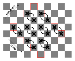
Figure 11: On a rotated $L_{1}\times L_{2}$ grid (here, $4\times 5$), we can implement an odd-even pattern of swaps on data qubits (gray) using ancillas (white). Row-wise and column-wise swaps used in swap routing on a grid [ACG94] can be modified as shown above so that ancilla used for swaps do not overlap. Therefore, any arbitrary permutation on a rotated grid of can be implemented in space-time $4(L_{1}+1)+2(L_{2}+1)$.

The first step of the swap-based compilation algorithm is to assign each of the input circuit’s qubits to a data qubit in the layout. Then, the gates in the input circuit are collected together into sets of disjoint gates. Before each set of gates, a permutation built from swap-gates is applied, which re-positions the qubits so that the gates in the set can be applied locally. We assume that the available local operations are the same as for our EDPC algorithm. In particular, we assume that the rotation gates ($S$, $T$, $S_{x}$ and $T_{x}$) can only be implemented at the boundary and that other single-qubit operations are performed as described in Section 2.1. One exception is that we make the simplifying assumption that the Hadamard can be performed without the need of three ancilla patches to simplify our analysis – this assumption could lead to an underestimate of the resources required for this swap-based compilation algorithm.

Input : A circuit $\mathcal{C}$ with all Paulis commuted to the end and merged with measurement

1 function cost(mapping $\pi$, vertices $v_{1},v_{2}$):

2      return depth and edge attaining $\min_{e\in\mathcal{M}}\text{{{depth(}}{{{{route(}}{{$\pi+\{v_{1}\mapsto e_{1},v_{2}\mapsto e_{2}\}$}}{{)}}}}{{)}}}$

3while available gates in $\mathcal{C}$ :

4      $\mathcal{G}\leftarrow$ available gates in $\mathcal{C}$;

5       execute all Hadamards and measurements in $\mathcal{G}$;

6      

7      $G\leftarrow$ surface code grid graph;

8       $\pi\leftarrow$ empty mapping of $V(G)\to V(G)$;

       // Start modification for operations requiring magic states

9       Set $B\subseteq V(G)$ as the set of boundary vertices;

10       $\mathcal{G}_{m}\leftarrow\{g\in\mathcal{G}\mid g\text{ is }S,T,S_{x},T_{x}\}$;

11       while $\mathcal{G}_{m}\not=\emptyset$ and $B\not=\emptyset$ :

12            $g\leftarrow$ pop random gate from $\mathcal{G}_{m}$;

13             $\pi\leftarrow\pi+\{v\mapsto u\}$, for closest $u\in B$ to $v$;

14             remove $u$ from $B$ and $G$;

15            

      // End modification

16       $\mathcal{M}\leftarrow$ maximum matching of $G$;

17       $\mathcal{G}_{c}=\{g\in\mathcal{G}\mid g\text{ is }{\textsc{cnot}}{}\}$;

18       while $G_{c}\not=\emptyset$ and $\mathcal{M}\not=\emptyset$ :

19            $g^{*},e^{*}\leftarrow\max_{g\in\mathcal{G}_{c}}$ cost($\pi+\{v_{1}\mapsto e_{1},v_{2}\mapsto e_{2}\}$) for $v_{1},v_{2}$ current location of $g$;

20             $\pi\leftarrow\pi+\{v_{1}\mapsto e_{1},v_{2}\mapsto e_{2}\}$, for $v_{1},v_{2}$ current location of $g^{*}$;

21             remove $g^{*}$ from $\mathcal{G}_{c}$;

22             remove $e^{*}$ from $\mathcal{M}$;

23            

24      execute the swaps found by route($\pi$);

25       execute gates on qubits mapped by $\pi$ since they are now local;

26      

Algorithm 6.1 swap compilation: We construct an algorithm based on the greedy depth mapper algorithm from [CSU19]. Let us implicitly define route($\pi$), for mapping $\pi$, which finds a swap circuit for implementing partial permutations [CSU19]. We can compute the required partial permutation from the current mapping of qubits, and the given future mapping $\pi$.

There are two main components of our swap-based algorithm which remain to be specified: how the permutations are implemented, and how we choose to separate the input circuit into a sequence of sets of disjoint gates. To permute the positions of data qubits, sequences of swap operations are used. Any permutation of the $n$ vertices in a square grid can be achieved in at most $3\sqrt{n}$ rounds of nearest-neighbor swaps [SHT19]. To do this involves three stages, with the first and third stages each involving rounds of swap-gates within rows only, and the second stage involving rounds of swap-gates within columns only. A round of swap-gates within either rows only or within columns only are implemented with surface code operations as shown in Figure 11. This immediately shows that this approach is asymptotically tight for parallel circuits because the depth of a swap-based approach is lower bounded by the $\sqrt{n}$ diameter of the architecture grid for one long-range cnot or rotation gate from the center of the grid. Therefore a parallel input circuit is compiled by the swap-based algorithm to an output circuit with depth $\Theta(\sqrt{n})$, including all the examples in Table 1.

There is considerable freedom in how to collect together gates from the input circuit into sets of disjoint gates. In our implementation in Algorithm 6.1, we use the greedy depth mapper algorithm from [CSU19], with a small modification to ensure that $S$ and $T$ gates are performed at the boundary. This algorithm also incorporates some further optimizations as described in [CSU19], including a partial mapping of qubits to locations, leaving the remaining qubits to go anywhere in an attempt to minimize the swap circuit depth.

6.4 Numerical results

Figure 12: Space-time cost of a randomly sampled set of disjoint cnots with standard error of the mean (shaded region) compiled to the surface code using EDPC and swap compilation. We generate 10 random circuits for each number of qubits ($n$) consisting of a set of disjoint cnots of varying density; the number of randomly selected qubits involved in a cnot is given by $n_{{\textsc{cnot}}{}}$. At all densities we see improved performance and scaling using EDPC.

Here we numerically compare the performance of EDPC with the swap-based compilation algorithm (Algorithm 6.1) when applied to a number of different input circuits. Note that our implementation of the EDPC compilation algorithm here differs slightly from that given in Algorithm 5.1, by greedily executing cnots earlier where possible. See Appendix E for details of the implementation.

Our first input circuit example consists of random parallel cnot circuits of different gate densities. The density $n_{\textsc{cnot}}{}$ of a circuit is how many of the data qubits are involved in a cnot gate in any such set. Therefore, $n_{\textsc{cnot}}{}=0.1n$ means that $10\%$ of all qubits ($n$) are performing a cnot gate in each set. For each data point, we sample 10 random circuits and plot the mean space-time cost in Figure 12 with the standard error of the mean in the shaded region. The runtime of the swap protocol was bounded by 2 days, which was insufficient for larger instances of these random circuits at high densities.

(a) Half $\textsc{c}^{8}\kern-0.90005pt\textsc{not}$

(b) Compilation of half $\textsc{c}^{k}\kern-0.90005pt\textsc{not}$

Figure 13: We compare the space-time cost of compiling a $T$-gate optimized circuit decomposition for a half $\textsc{c}^{k}\kern-0.90005pt\textsc{not}$ circuit to the surface code using EDPC and swap compilation. We see in the log-log plot (13(b)) that dependence of the space-time cost on $n$ gives a higher scaling dependence in the case of swap compilation than EDPC. This results a lower space-time cost for EDPC starting from 64 qubits.

We also consider a more structured input circuit, namely implementing half of a multi-controlled-$X$ gate, $\textsc{c}^{k}\kern-1.00006pt\textsc{not}$. We consider decompositions of $\textsc{c}^{k}\kern-1.00006pt\textsc{not}$ for $k$ integer powers of $2$, but only compile the first half of the circuit, given in Figure 13(a). A $T$-efficient implementation of $\textsc{c}^{k}\kern-1.00006pt\textsc{not}$ uses measurement and feedback for uncomputation [Jon13], which are not captured in our model (see Section 7). We plot the space-time cost of compiling the half $\textsc{c}^{k}\kern-1.00006pt\textsc{not}$ in Figure 13(b). We see that the dependence on the number of qubits $k$ is worse for swap-based compilation, and results in a larger space-time cost starting at 64 qubits. Unfortunately, the swap-based compilation is quite slow: we ran the algorithm for at most 3 days and 9 hours at each data point and were only able to obtain results up to 128 qubits. However, the data we were able to obtain indicates a cross-over for compiling $\textsc{c}^{k}\kern-1.00006pt\textsc{not}$ circuits. The swap-based compilation has better space-time performance for small instances, while EDPC has a better space-time performance for compiling large $\textsc{c}^{k}\kern-1.00006pt\textsc{not}$ circuits.

7 Conclusion

In this paper, we have introduced the EDPC algorithm for the compilation of input quantum circuits into operations which can be implemented fault-tolerantly with the surface code. The heart of this algorithm lies in the EDP subroutine, which can implement both sets of parallel long-range cnot gates and sets of parallel rotations in constant depth using existing efficient graph algorithms to find sets of edge-disjoint paths. EDPC has advantages over other compilation approaches including Pauli-based computation, network coding based compilation, and swap-based compilation. We numerically find that EDPC significantly outperforms swap-based circuit compilation in the space-time cost of random cnot circuits for a broad range of instances, and for larger $\textsc{c}^{k}\kern-1.00006pt\textsc{not}$ gates. However, many details of EDPC can be improved, as it is only a first step towards using long-range operations for surface code compilation.

EDPC requires sets of constrained edge-disjoint paths, which we call operator paths and run almost entirely along ancilla qubits. Better algorithms for finding maximum sets of edge-disjoint operator paths could improve EDPC. It seems likely that an $O(\log n)$-approximation algorithm for finding maximum EDP sets on grids [AR95] can be modified to give an algorithm for finding maximum sets of edge-disjoint operator paths on grids. A polylogarithmic approximation algorithm for this task would imply an approximation algorithm for minimizing the depth, up to a polylogarithmic factor, of compiling parallel cnots using the EDP subroutine. In practice, it is, however, also important to find approximation algorithms with reasonable constant prefactors.

The runtime complexity of EDPC for an input circuit of depth $D$ acting on $n$ qubits is $O(Dn^{3}\log n)$. This is significantly faster than the swap-based compilation in Section 6.3, which was found to be $O(Dn^{5})$ in [CSU19]. We found that our implementation of the swap-based compilation implementation runtime is much slower than that of EDPC on small instances, and found that the swap-based algorithm had impractically long runtimes when applied to circuits beyond a few hundred qubits, the regime of large-scale applications of quantum algorithms [Rei+17, GE21]. Potential ways to further improve EDPC’s runtime include using a dynamical decremental all-pair shortest path algorithm in the greedy approximation of the maximum EDP set, or by finding faster and better approximation algorithms for finding the maximum set of edge-disjoint operator paths.

Any diagonal gates in the $Z$ (or $X$) basis can be performed remotely on the boundary, including CCZ gates [GF19] (see Appendix D). Therefore, our results on applying $Z(\theta)$ rotations can be extended to diagonal gates, which will benefit circuit depth.

Even with the capability to perform long-range operations it may still be helpful to localize the quantum information on some part of the architecture such as by permuting the data qubits. In particular, the size of the EDP set is bounded above by the minimum edge cut separating the terminals. Therefore, it may be beneficial to first redistribute quantum information where it is needed to ensure large EDP solutions exist. It is straightforward to construct a long-range move of a data qubit to an ancilla in depth 2 from a long-range cnot, by performing the cnot targeting a $|0\rangle$ ancilla state and measuring the source in the $X$ basis up to Pauli corrections. It also is straightforward to adapt the EDP subroutine to perform sets of these long-range moves along operator paths, now ending at the ancilla, in depth 4. The depth to permute only a few qubits a long distance can be improved significantly by this technique. For example, a swap of the two corners of an $L\times L$ grid architecture takes $O(1)$ depth using long-range moves, as opposed to $\Omega(L)$ depth using conventional swaps. It remains an open question how to trade off permuting data qubits (using swaps or long-range moves) and directly using long-range cnots.

We have assumed that classical feedback is not present in the input circuit for clarity of presentation. EDPC can readily be extended to the setting of classical feedback in the input circuit to form a “just-in-time” surface code compilation algorithm. To do so, a larger computation would be broken up into a sequence of circuit executions without classical feedback, where prior measurement results specify the next circuit to compile and execute.

Acknowledgements

We would like to thank Alexander Vaschillo and Dmitry Vasilevsky for helpful discussion, and Thomas Haner for coming up with a simple correctness proof for delayed remote execution gadget and many helpful discussions. A slightly modified version of this proof is presented in Appendix D.

E.S. acknowledges support by a Microsoft internship, an IBM PhD Fellowship, and the U.S. Department of Energy, Office of Science, Office of Advanced Scientific Computing Research, Quantum Testbed Pathfinder program (award number DE-SC0019040).

Appendix A Surface code architecture

Here we review some basic details of the surface code focusing on the elementary logical operations shown in Figure 1. This is intended as a high-level overview to provide some intuition of how the logical operations in Figure 1 arise and what their resource costs are. For more thorough reviews of surface codes see Refs. [Bom13, Fow+12, Bro+17].

To implement the surface code, we assume physical qubits are laid out on the vertices of a 2D grid, with nearest-neighbor interactions allowed. For concreteness, we will describe here an implementation of lattice surgery with the rotated surface code with half-moon boundary [LR14], although our EDPC algorithm can use other implementations. A single surface code patch encodes a single logical qubit in $2d^{2}-1$ physical qubits, where the odd parameter $d$ is known as the code distance which corresponds to the level of noise protection; see Figure 14(a). For clarity, within this section of the appendix we refer to physical qubits and logical qubits explicitly, however in other sections we often drop the word “logical” when referring to logical qubits for brevity.

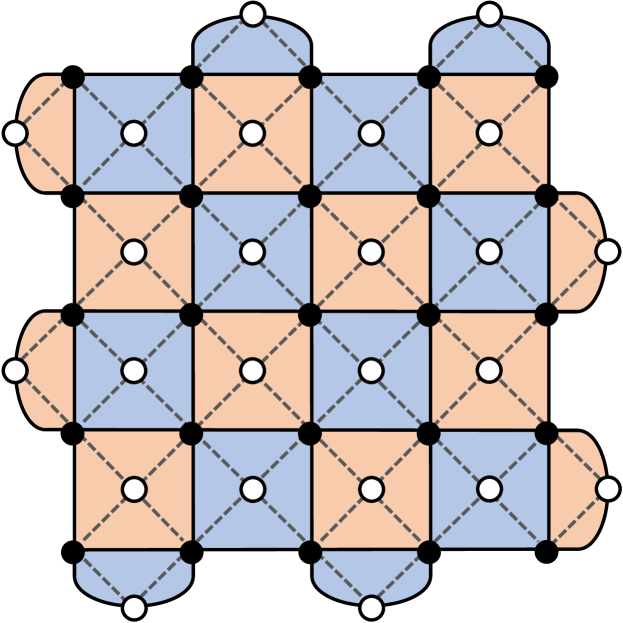
(a) Surface code patch

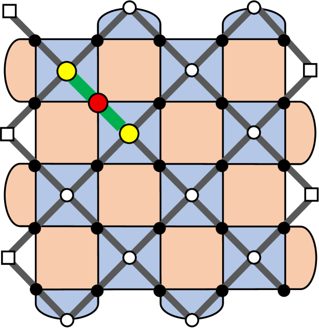
(b) $X$-Stabilizer decoding graph

Figure 14: (a) A $d=5$ surface code patch implemented in a grid of data physical qubits (black disks), and ancilla physical qubits (white disks). Error correction is implemented with single-qubit operations and cnot between pairs of qubits connected by a dashed edge. $Z$ and $X$ type stabilizers are associated with alternating red and blue faces. (b) A decoding graph that is defined by associating an edge with each qubit and a vertex for each stabilizer. If stabilizers are measured perfectly, $Z$ errors on data qubits (marked in red) can be corrected by finding a minimum weight matching (green edges) of vertices associated with unsatisfied $X$ stabilizers (yellow disks).

We designate every odd physical qubit as a data physical qubit in the patch, and every even physical qubit as an ancilla physical qubit to facilitate a stabilizer measurement; see Figure 14(a). The code space of a surface code consists of those states of the data physical qubits which are simultaneous $+1$ eigenstates of the set of stabilizer generators. The stabilizer generators can be associated with faces and are either $X\otimes X\otimes X\otimes X$ or $Z\otimes Z\otimes Z\otimes Z$ operators for the bulk (interior) of the code or $X\otimes X$ or $Z\otimes Z$ operators on the boundary. We can see that the logical $Z$ operator, $Z_{L}$, defined as any path of single-qubit $Z$ operators on physical qubits connecting the rough boundaries, commutes with all stabilizers. Similarly, the logical $X$ operator, $X_{L}$, is a path of $X$ operators connecting the smooth boundaries.

For quantum error correction, it is necessary to repeatedly measure stabilizer generators. Stabilizer generators can be measured by running small circuits consisting of the preparation of the ancilla physical qubit, cnots between the ancilla physical qubit and the data physical qubits, followed by measurement of the ancilla physical qubit. Error correction can be performed by associating qubits with edges and stabilizer generators with vertices of a so-called decoding graph; see Figure 14(b). A classical algorithm known as a decoder is used to infer a set of edges (specifying the support of the X or Z correction) given a subset of vertices (corresponding to unsatisfied Z or X stabilizers, that is stabilizer generators with measurement outcome -1). Figure 14(b) shows an example of this in the setting of perfect stabilizer measurements, although this can be generalized to handle faulty measurements by repeating measurements.

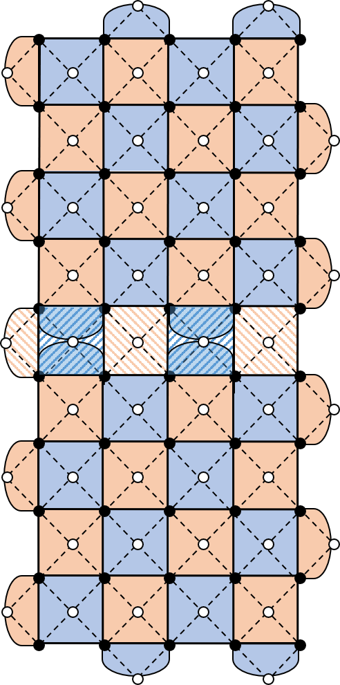
(a) Logical $Z_{L}\otimes Z_{L}$ measurement

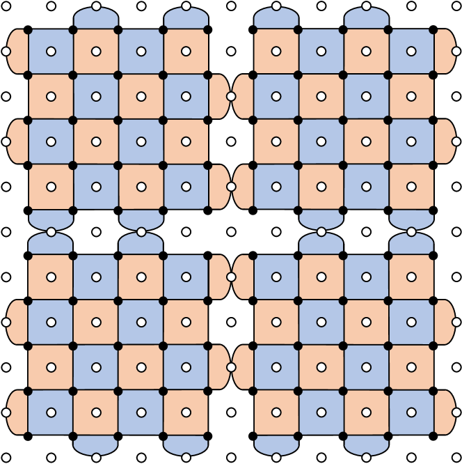
(b) Patches tiling the plane

Figure 15: (a) A logical $Z_{L}\otimes Z_{L}$ measurement is performed by lattice surgery in the following steps: (i) Stop measuring the weight-two stabilizers along the horizontal boundary between the patches. (ii) Reliably measure the bulk faces for a single vertically-extended patch. Note that $Z_{L}\otimes Z_{L}$ can be inferred from the product of the outcomes of the newly measured red faces. This temporarily merges the patches to form a single extended surface code patch. (iii) Reliably measure once more the weight-two faces along the horizontal boundary between the patches. This separates the pair of patches. (b) Two types of patches tile the plane, with $Z_{L}\otimes Z_{L}$ measurements possible between vertically neighboring patches, and $X_{L}\otimes X_{L}$ measurements possible between horizontally neighboring patches.

Logical operations can be implemented fault-tolerantly on logical qubits encoded in surface codes. For example, a destructive logical $X$ measurement of a patch is implemented by measuring all data qubits in the $X$ basis, and then using a decoder to process the physical outcomes and reliably identify the logical measurement outcome. Another important logical operation is the non-destructive measurement of a logical joint Pauli operator using an approach known as lattice surgery [Hor+12] as shown in Figure 15(a). To simplify lattice surgery by lining up the boundary stabilizers of neighboring patches, we consider a tiling of the plane using two versions of distance $d$ surface code patches as shown in Figure 15(b) which forms a grid of logical qubits. Logical $Z_{L}\otimes Z_{L}$ can be measured between vertical neighbor patches while $X_{L}\otimes X_{L}$ can be measured between horizontal neighbor patches.

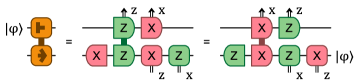
Figure 16: The move operation can be implemented in depth 1 by local and neighboring Pauli measurements. A horizontal move can be implemented by preparing a single-qubit patch in $|0\rangle$, applying joint $XX$ measurement, and then measuring the original patch in the $Z$ basis (up to Pauli corrections). The vertical move follows from applying a Hadamard to the source qubit $|\phi\rangle$ and a Hadamard on the output. Simplifying the circuit gives the right-hand side in the Figure, with a $ZZ$ measurement that is available vertically.

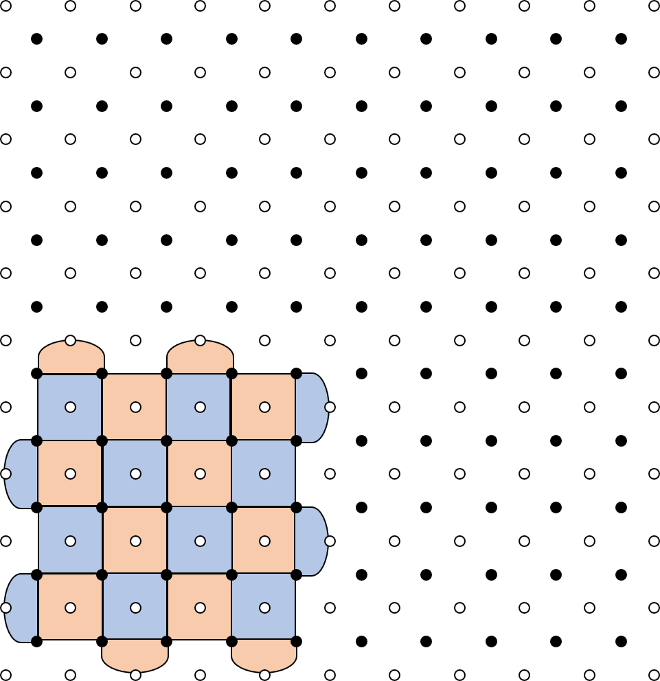
(a) Transversal Hadamard

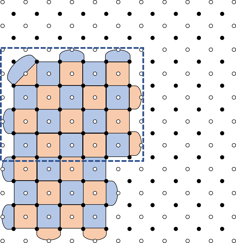
(b) Extended patch

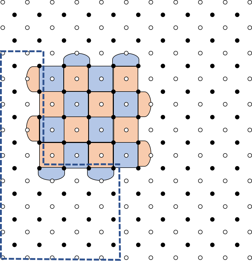
(c) Shrunk patch

Figure 17: Implementation of a Hadamard operation in depth 3 with three ancilla patches. (17(a)) A transverse Hadamard is applied in depth 0 to each physical data qubit, which switches the arrangement of $X$ and $Z$ stabilizer generators compared to the standard configuration. (17(b)) The patch is extended in depth 1 so that a segment of the standard boundary type is introduced on the right. (17(c)) The patch is shrunk into a standard surface code patch of the form of the top-left corner of the region (see Figure 15(b)) in depth 1, but with its location shifted by a (code distance) $d$-independent amount. This allows us to shift the patch into the top-left corner in 0 depth (not shown). Then we move the logical qubit to the bottom-left corner in depth 1.

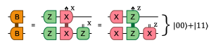
(a) Bell pair preparation

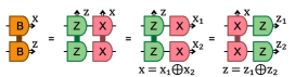
(b) Bell measurement

Figure 18: We can implement Bell preparation and measurement in terms of single and two-qubit Pauli measurements in depth 1 as given in Figure 18 [Lit19]. (18(a)) A Bell pair can be prepare from a (horizontal) joint $XX$ measurement of $|00\rangle$ or a (vertical) joint $ZZ$ measurement of $|++\rangle$, up to Pauli corrections. (18(b)) A destructive Bell measurement can be implemented by a joint $XX$ measurement followed by individual $Z$ basis measurements, or by a joint $ZZ$ measurement followed by individual $X$ basis measurements.

The allowed fault-tolerant logical operations that we assume throughout the paper and the resources they require are listed in Figure 1. These are largely based on the rules specified in [Lit19]. Here we justify the resource requirements for the logical operations in Figure 1 not covered in [Lit19] on a distance-$d$ surface code. For space analysis, we work in units of full surface code patches such that if any qubits from a patch are needed to implement an operation the full patch is counted. We show how to implement the operations in terms of more elementary Pauli measurements. The move operation can be implemented in depth 1 with the target qubit as ancilla, as shown in Figure 16. The Hadamard can be implemented in depth three with three ancilla patched along with the move operation as shown in Figure 17. Finally, Bell measurement and preparation can be implemented in depth 1 as shown in Figure 18.

It is worth mentioning that there is considerable freedom in the detailed choice and implementation of the surface code which could have an impact on the space-time cost of logical operations, both at the physical level but also in some cases at the logical level. For example the Hadamard could be performed using just one logical ancilla patch if each patch was padded with extra qubits. We do not explore these alternatives here, but note that our EDPC algorithm can still be applied if these alternatives are used.

Appendix B Logical space time cost as a proxy for physical space time cost

Here we provide a justification for our use of logical space time cost as a proxy for physical space time cost. As we have seen in Figure 1 and Appendix A, logical operations implemented with the surface code require physical time that scales as $d$ and physical space that scales as $d^{2}$. For a logical circuit written in terms of a total of $A_{\text{logical}}$ elementary logical operations implemented using surface codes of distance $d$, the physical space-time cost $A_{\text{physical}}$ is approximately

$$A_{\text{physical}}\sim A_{\text{logical}}d^{3}.$$ (8)

The probability of any of these elementary operations resulting in a logical failure scales as $p_{\text{fail}}\sim(p/p^{*})^{d/2}$, where the fixed system parameters are the physical error rate $p$, and the fault-tolerant threshold for the surface code $p^{*}$. Moreover, we assume $p_{\text{fail}}\sim 1/A_{\text{logical}}$ to ensure that the logical circuit is reliable with as small a code distance as possible. This suggests that the code distance behaves as

$$d\sim\frac{2\log A_{\text{logical}}}{\log p^{*}-\log p}.$$ (9)

Therefore we see that the physical and logical space time costs are monotonically related, i.e.,

$$A_{\text{physical}}\sim A_{\text{logical}}(\log A_{\text{logical}})^{3}.$$ (10)

Appendix C cnot via Bell operations

We list more variations of the standard cnot gate (Figure 3(a)) that use intermediate Bell preparation and measurements on ancillas in Figure 19. By choosing the right subcircuit, we see that the long-range operations in Figure 8 implement a cnot gate.

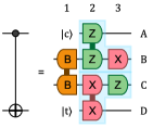
(a) cnot via Bell preparation

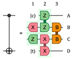
(b) cnot via Bell measure

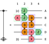
(c) cnot with control first

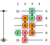
(d) cnot with target first

Figure 19: Various implementations of a cnot gate with intermediate ancilla qubits and Bell operations. In particular, we are able to apply the control and the target either before (green) or after (teal) Bell preparation and measurement steps, while keeping the depth at 2.

Appendix D Remote execution of diagonal gates

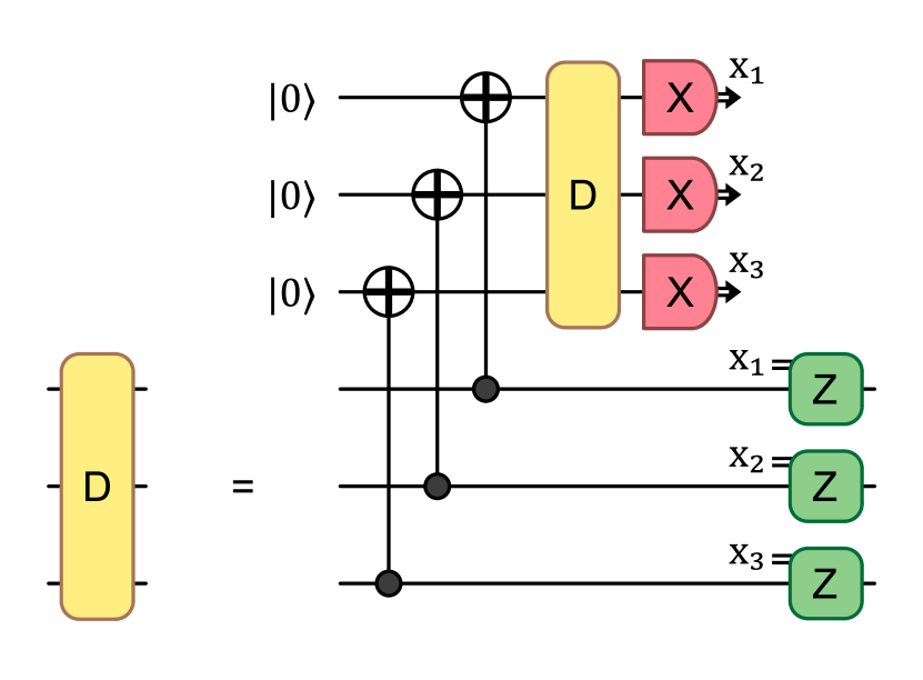
(a) Diagonal gate in computational basis

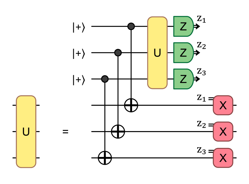
(b) Diagonal gate in Hadamard basis

Figure 20: (20(a)) Any $k$-qubit gate diagonal in the computational basis can be remotely executed on $k$ dedicated ancilla by first using cnots. We use this technique to apply remote $Z(\theta)$ rotations (Figure 10(b)) with magic states at the boundary. (20(b)) Similarly, gates diagonal in the Hadamard basis also have a remote implementation. Since the Pauli corrections can be commuted through Clifford circuits, Clifford circuits can be executed immediately after executing the cnot operations with no need to wait on the remote operations.

A gate $D$ diagonal on $k$ source qubits in the computational basis can be executed on $k$ ancilla by first entangling these ancilla qubits using cnots. We call this remote execution. Let the computational basis be $|\ell\rangle$, for $\ell\in[2^{k}]$, then $D|\ell\rangle=\exp(i\phi_{\ell})|\ell\rangle$. We saw one use for remote gates in applying rotations at the boundary requiring magic states (Section 4).

We execute $D$ remotely as follows (see Figure 20). First, we initialize the ancilla in the state $|0\rangle^{\otimes k}$. Let the source qubits be in some pure state $\sum_{\ell}\alpha_{\ell}|\ell\rangle$, for $\alpha_{\ell}\in\mathbb{C}$. then we apply $k$ transversal cnot gates controlled on source qubits so that the overal state becomes $\sum_{\ell}\alpha_{\ell}|\ell\rangle\otimes|\ell\rangle$. We now apply $D$ to the ancilla instead

$$(\mathbbm{1}\otimes D)\sum_{\ell}\alpha_{\ell}|\ell\rangle\otimes|\ell\rangle=\sum_{\ell}\alpha_{\ell}\exp(i\phi_{\ell})|\ell\rangle\otimes|\ell\rangle.$$ (11)

We now disentangle the ancilla by measuring them in the $X$ basis. Let the measurement give outcomes $\mathbf{x}\in\{0,1\}^{k}$, then the state on the source qubits is mapped to

$$\sum_{\ell}\alpha_{\ell}\exp(i\phi_{\ell})(-1)^{(\mathbf{x},\ell)}|\ell\rangle,$$ (12)

where $(\mathbf{x},\ell)$ is the inner product modulo 2 between $\mathbf{x}$ and the binary representation of $\ell$. Applying a $Z$ correction to each qubit $j\in[k]$ controlled on measurement result $\mathbf{x}_{j}$ maps the state to $\sum_{\ell}\alpha_{\ell}\exp(i\phi_{\ell})|\ell\rangle$ as required.

This technique can be extended to any unitary operator $U$ since it can be unitarily diagonalized as $U=VDV^{\dagger}$ by the spectral theorem, for $V$ unitary and $D$ diagonal operators. A particularly simple case are unitary operators that are diagonal in the Hadamard basis, where $V=H^{\otimes k}$. We write $U=H^{\otimes k}DH^{\otimes k}$ on the source qubits and apply remote execution of $D$ using our techniques above. We then simplify the circuit to obtain Figure 20(b).

Appendix E EDPC implementation

Here we provide Algorithm E.1, which specifies the implementation of EDPC used for our numerical results presented in Section 6.4, here called EDPCI for clarity. EDPCI differs slightly from EDPC (Section 5) and we will highlight the differences. Up until Algorithm E.1 in Algorithm E.1, EDPCI is the same as EDPC. Then, EDPCI greedily attempts to execute long-range cnots earlier than would occur in EDPC. In particular, EDPC only executes cnots after all available rotations have been executed, whereas EDPCI finds a set $\mathcal{P}_{c}$ on Algorithm E.1 such that $\mathcal{P}_{c}\cup\mathcal{P}_{m}$ forms an EDP set. Now EDPCI concurrently executes long-range cnots using any edges left over from remote rotations. Moreover, we note that EDPC uses the bounded $\mathcal{T}$-operator set algorithm (Algorithm 3.2) to execute a parallel cnot circuit, which additionally finds a bounded $\mathcal{T}$-operator set $\mathcal{Q}_{1}$ on Algorithm 3.2, whereas EDPCI only finds $\mathcal{Q}_{2}$ from the bounded $\mathcal{T}$-operator set algorithm if given a parallel cnot circuit. As a consequence of this difference, while a parallel input cnot circuit is guaranteed to compile to an output circuit upper bounded by $O(\sqrt{n})$, EDPCI does not have this guarantee.

Input : Circuit $\mathcal{C}$ with Paulis commuted to the end and merged with measurement

1

2while available operations in $\mathcal{C}$ :

3      execute all available state preparation, measurement, and Hadamard;

4      

5      $\mathcal{G}_{m}\leftarrow\{\text{available operations }g\in\mathcal{C}\mid g\text{ is }S,T,S_{x},$ or $T_{x}\}$;

6       $\mathcal{G}_{c}\leftarrow\{\text{available operations }g\in\mathcal{C}\mid g\text{ is {{cnot}}{}}\}$;

7       while $\mathcal{G}_{m}\cup\mathcal{G}_{c}\neq\emptyset$ :

8            $G\leftarrow$ surface code grid graph;

             $\mathcal{P}_{m}\leftarrow$ max_rotations($\mathcal{G}_{m}$);

              // see Algorithm 4.1

9             remove edges in each $P\in\mathcal{P}_{m}$ from $G$;

10            

11            $\mathcal{P}_{c}\leftarrow$ approximate max operator EDP set on $G$ with $\mathcal{G}_{c}$;

12            

13            execute concurrent remote rotations along $\mathcal{P}_{m}$ and long-range cnots along $\mathcal{P}_{c}$ using EDP subroutine;

14             remove executed rotations from $\mathcal{G}_{m}$ and cnots from $\mathcal{G}_{c}$;

15            

Algorithm E.1 EDPC implementation: The EDPC algorithm (Algorithm 5.1) differs from our implementation in that it greedily tries to execute cnots earlier.

References

- [Ahl+00] Rudolf Ahlswede, Ning Cai, Shuo-Yen Robert Li and Raymond W. Yeung “Network information flow” In IEEE Transactions on Information Theory 46.4 Institute of ElectricalElectronics Engineers (IEEE), 2000, pp. 1204–1216 DOI: 10.1109/18.850663
- [ACG94] Noga Alon, F… Chung and R.. Graham “Routing Permutations on Graphs via Matchings” In SIAM Journal on Discrete Mathematics 7.3 Society for Industrial & Applied Mathematics (SIAM), 1994, pp. 513–530 DOI: 10.1137/s0895480192236628
- [AR95] Yonatan Aumann and Yuval Rabani “Improved Bounds for All Optical Routing” In Proceedings of the Sixth Annual ACM-SIAM Symposium on Discrete Algorithms, SODA ’95 3600 University City Science Center, Philadelphia, PA, United States: Society for IndustrialApplied Mathematics, 1995, pp. 567–576
- [BR17] Indranil Banerjee and Dana Richards “New Results on Routing via Matchings on Graphs” In Fundamentals of Computation Theory, Lecture Notes in Computer Science 10472 Berlin, Germany: Springer, 2017, pp. 69–81 DOI: 10.1007/978-3-662-55751-8_7
- [Bap+22] Aniruddha Bapat, Andrew M. Childs, Alexey V. Gorshkov and Eddie Schoute “Advantages and limitations of quantum routing”, 2022 arXiv:2206.01766 [quant-ph]
- [BH20] Niel Beaudrap and Steven Herbert “Quantum linear network coding for entanglement distribution in restricted architectures” In Quantum 4 Verein zur Forderung des Open Access Publizierens in den Quantenwissenschaften, 2020, pp. 356 DOI: 10.22331/q-2020-11-01-356
- [Ben+03] C.. Bennett, A.. Harrow, D.. Leung and J.. Smolin “On the capacities of bipartite hamiltonians and unitary gates” In IEEE Transactions on Information Theory 49.8 Institute of ElectricalElectronics Engineers (IEEE), 2003, pp. 1895–1911 DOI: 10.1109/tit.2003.814935
- [Bom13] H. Bombin “Topological Codes” In Quantum Error Correction Cambridge: Cambridge University Press, 2013 arXiv:1311.0277 [quant-ph]
- [BK98] S.. Bravyi and A.. Kitaev “Quantum codes on a lattice with boundary”, 1998 arXiv:quant-ph/9811052v1 [quant-ph]
- [BK05] Sergey Bravyi and Alexei Kitaev “Universal quantum computation with ideal Clifford gates and noisy ancillas” In Physical Review A 71.2 American Physical Society (APS), 2005, pp. 022316 DOI: 10.1103/physreva.71.022316
- [Bri+98] H.-J. Briegel, W. Dür, J.. Cirac and P. Zoller “Quantum Repeaters: The Role of Imperfect Local Operations in Quantum Communication” In Physical Review Letters 81.26 American Physical Society, 1998, pp. 5932–5935 DOI: 10.1103/physrevlett.81.5932
- [Bro+17] Benjamin J. Brown, Katharina Laubscher, Markus S. Kesselring and James R. Wootton “Poking Holes and Cutting Corners to Achieve Clifford Gates with the Surface Code” In Physical Review X 7.2 American Physical Society (APS), 2017, pp. 021029 DOI: 10.1103/physrevx.7.021029
- [CC21] Christopher Chamberland and Earl T. Campbell “Universal quantum computing with twist-free and temporally encoded lattice surgery”, 2021 arXiv:2109.02746 [quant-ph]
- [Cha+20] Christopher Chamberland, Guanyu Zhu, Theodore J. Yoder, Jared B. Hertzberg and Andrew W. Cross “Topological and Subsystem Codes on Low-Degree Graphs with Flag Qubits” In Physical Review X 10.1 American Physical Society, 2020, pp. 011022 DOI: 10.1103/physrevx.10.011022
- [Cha+20a] Rui Chao, Michael E. Beverland, Nicolas Delfosse and Jeongwan Haah “Optimization of the surface code design for Majorana-based qubits” In Quantum 4 Verein zur Förderung des Open Access Publizierens in den Quantenwissenschaften, 2020, pp. 352 DOI: 10.22331/q-2020-10-28-352
- [CKS06] Chandra Chekuri, Sanjeev Khanna and F. Shepherd “An Approximation and Integrality Gap for Disjoint Paths and Unsplittable Flow” In Theory of Computing 2.1 Theory of Computing Exchange, 2006, pp. 137–146 DOI: 10.4086/toc.2006.v002a007
- [CSU19] Andrew M. Childs, Eddie Schoute and Cem M. Unsal “Circuit Transformations for Quantum Architectures” In 14th Conference on the Theory of Quantum Computation, Communication and Cryptography (TQC 2019) 135, Leibniz International Proceedings in Informatics (LIPIcs) Dagstuhl, Germany: Schloss Dagstuhl–Leibniz-Zentrum fuer Informatik, 2019, pp. 3:1–3:24 DOI: 10.4230/LIPIcs.TQC.2019.3
- [CK15] Julia Chuzhoy and David H.. Kim “On Approximating Node-Disjoint Paths in Grids” In Approximation, Randomization, and Combinatorial Optimization. Algorithms and Techniques (APPROX/RANDOM 2015) 40, Leibniz International Proceedings in Informatics (LIPIcs) Dagstuhl, Germany: Schloss Dagstuhl–Leibniz-Zentrum fuer Informatik, 2015, pp. 187–211 DOI: 10.4230/LIPIcs.APPROX-RANDOM.2015.187
- [CKN18] Julia Chuzhoy, David H.. Kim and Rachit Nimavat “Almost polynomial hardness of node-disjoint paths in grids” In Proceedings of the 50th Annual ACM SIGACT Symposium on Theory of Computing - STOC 2018 ACM Press, 2018 DOI: 10.1145/3188745.3188772
- [DBT21] Nicolas Delfosse, Michael E. Beverland and Maxime A. Tremblay “Bounds on stabilizer measurement circuits and obstructions to local implementations of quantum LDPC codes”, 2021 arXiv:2109.14599 [quant-ph]
- [FF56] L.. Ford and D.. Fulkerson “Maximal Flow Through a Network” In Canadian Journal of Mathematics 8 Canadian Mathematical Society, 1956, pp. 399–404 DOI: 10.4153/cjm-1956-045-5
- [Fow+12] Austin G. Fowler, Matteo Mariantoni, John M. Martinis and Andrew N. Cleland “Surface codes: Towards practical large-scale quantum computation” In Physical Review A 86.3 American Physical Society, 2012, pp. 032324 DOI: 10.1103/PhysRevA.86.032324
- [FC16] Amir Fruchtman and Iris Choi “Technical Roadmap for Fault-Toleran Quantum Computing”, 2016 URL: https://nqit.ox.ac.uk/content/technical-roadmap-fault-tolerant-quantum-computing.html
- [GE21] Craig Gidney and Martin Ekerå “How to factor 2048 bit RSA integers in 8 hours using 20 million noisy qubits” In Quantum 5 Verein zur Förderung des Open Access Publizierens in den Quantenwissenschaften, 2021, pp. 433 DOI: 10.22331/q-2021-04-15-433
- [GF19] Craig Gidney and Austin G. Fowler “Flexible layout of surface code computations using AutoCCZ states”, 2019 arXiv:1905.08916 [quant-ph]
- [HPE19] Frederik Hahn, A. Pappa and Jens Eisert “Quantum network routing and local complementation” In npj Quantum Information 5, 2019, pp. 1–7 DOI: 10.1038/s41534-019-0191-6
- [Hor+12] Clare Horsman, Austin G. Fowler, Simon Devitt and Rodney Van Meter “Surface code quantum computing by lattice surgery” In New Journal of Physics 14.12 IOP Publishing, 2012, pp. 123011 DOI: 10.1088/1367-2630/14/12/123011
- [Jav+17] Ali Javadi-Abhari, Pranav Gokhale, Adam Holmes, Diana Franklin, Kenneth R. Brown, Margaret Martonosi and Frederic T. Chong “Optimized surface code communication in superconducting quantum computers” In Proceedings of the 50th Annual IEEE/ACM International Symposium on Microarchitecture ACM, 2017 DOI: 10.1145/3123939.3123949
- [Joh74] David S. Johnson “Approximation algorithms for combinatorial problems” In Journal of Computer and System Sciences 9.3 Elsevier BV, 1974, pp. 256–278 DOI: 10.1016/s0022-0000(74)80044-9
- [Jon13] Cody Jones “Low-overhead constructions for the fault-tolerant Toffoli gate” In Physical Review A 87.2 American Physical Society (APS), 2013, pp. 022328 DOI: 10.1103/physreva.87.022328
- [Kar+17] Torsten Karzig et al. “Scalable designs for quasiparticle-poisoning-protected topological quantum computation with Majorana zero modes” In Phys. Rev. B 95 American Physical Society, 2017, pp. 235305 DOI: 10.1103/PhysRevB.95.235305
- [Kit03] A.Yu. Kitaev “Fault-tolerant quantum computation by anyons” In Annals of Physics 303.1 Elsevier BV, 2003, pp. 2–30 DOI: 10.1016/s0003-4916(02)00018-0
- [KT95] J. Kleinberg and E. Tardos “Disjoint paths in densely embedded graphs” In Proceedings of IEEE 36th Annual Foundations of Computer Science IEEE Comput. Soc. Press, 1995 DOI: 10.1109/sfcs.1995.492462
- [KT06] Jon Kleinberg and Éva Tardos In Algorithm Design Boston: Pearson/Addison-Wesley, 2006
- [KT06a] Jon Kleinberg and Éva Tardos In Algorithm Design Boston: Pearson/Addison-Wesley, 2006
- [Kle96] Jon M. Kleinberg “Approximation algorithms for disjoint paths problems”, 1996 URL: http://hdl.handle.net/1721.1/11013
- [Kni04] E. Knill “Fault-Tolerant Postselected Quantum Computation: Schemes”, 2004 arXiv:quant-ph/0402171 [quant-ph]
- [Kni05] E. Knill “Quantum computing with realistically noisy devices” In Nature 434.7029 Springer ScienceBusiness Media LLC, 2005, pp. 39–44 DOI: 10.1038/nature03350
- [Kob+09] Hirotada Kobayashi, François Le Gall, Harumichi Nishimura and Martin Rötteler “General Scheme for Perfect Quantum Network Coding with Free Classical Communication” In Automata, Languages and Programming Springer Berlin Heidelberg, 2009, pp. 622–633 DOI: 10.1007/978-3-642-02927-1_52
- [Kob+11] Hirotada Kobayashi, François Le Gall, Harumichi Nishimura and Martin Rötteler “Constructing quantum network coding schemes from classical nonlinear protocols” In 2011 IEEE International Symposium on Information Theory Proceedings IEEE, 2011 DOI: 10.1109/isit.2011.6033701
- [KS04] Stavros G. Kolliopoulos and Clifford Stein “Approximating disjoint-path problems using packing integer programs” In Mathematical Programming 99.1 Springer ScienceBusiness Media LLC, 2004, pp. 63–87 DOI: 10.1007/s10107-002-0370-6
- [LR14] Andrew J. Landahl and Ciaran Ryan-Anderson “Quantum computing by color-code lattice surgery”, 2014 arXiv:1407.5103 [quant-ph]
- [Lao+18] L. Lao, B. Wee, I. Ashraf, J. Someren, N. Khammassi, K. Bertels and C.. Almudever “Mapping of lattice surgery-based quantum circuits on surface code architectures” In Quantum Science and Technology 4.1 IOP Publishing, 2018, pp. 015005 DOI: 10.1088/2058-9565/aadd1a
- [LL04] April Rasala Lehman and Eric Lehman “Complexity Classification of Network Information Flow Problems” In Proceedings of the Fifteenth Annual ACM-SIAM Symposium on Discrete Algorithms, SODA ’04 New Orleans, Louisiana: Society for IndustrialApplied Mathematics, 2004, pp. 142–150
- [LOW10] Debbie Leung, Jonathan Oppenheim and Andreas Winter “Quantum Network Communication—The Butterfly and Beyond” In IEEE Transactions on Information Theory 56.7 Institute of ElectricalElectronics Engineers (IEEE), 2010, pp. 3478–3490 DOI: 10.1109/tit.2010.2048442
- [Lit19] Daniel Litinski “A Game of Surface Codes: Large-Scale Quantum Computing with Lattice Surgery” In Quantum 3, 2019, pp. 128 DOI: 10.22331/q-2019-03-05-128
- [LO17] Daniel Litinski and Felix Oppen “Braiding by Majorana tracking and long-range CNOT gates with color codes” In Physical Review B 96.20 American Physical Society (APS), 2017, pp. 205413 DOI: 10.1103/physrevb.96.205413
- [Mur+19] Prakash Murali, Jonathan M. Baker, Ali Javadi Abhari, Frederic T. Chong and Margaret Martonosi “Noise-Adaptive Compiler Mappings for Noisy Intermediate-Scale Quantum Computers” In ASPLOS ’19 New York NY, United States: The Association for Computing Machinery, 2019, pp. 1015–1029 DOI: 10.1145/3297858.3304075
- [Rei+17] Markus Reiher, Nathan Wiebe, Krysta M. Svore, Dave Wecker and Matthias Troyer “Elucidating reaction mechanisms on quantum computers” In Proceedings of the National Academy of Sciences 114.29 National Academy of Sciences, 2017, pp. 7555–7560 DOI: 10.1073/pnas.1619152114
- [RS16] Neil J. Ross and Peter Selinger “Optimal ancilla-free Clifford+T approximation of z-rotations” In Quantum Information and Computation 16.11&12 Rinton Press, 2016, pp. 901–953 DOI: 10.26421/QIC16.11-12-1
- [SLI12] Takahiko Satoh, François Le Gall and Hiroshi Imai “Quantum network coding for quantum repeaters” In Physical Review A 86.3 American Physical Society (APS), 2012, pp. 032331 DOI: 10.1103/physreva.86.032331
- [SHT19] Damian S. Steiger, Thomas Häner and Matthias Troyer “Advantages of a modular high-level quantum programming framework” In Microprocessors and Microsystems 66 Elsevier BV, 2019, pp. 81–89 DOI: 10.1016/j.micpro.2019.02.003
- [WFH11] David S. Wang, Austin G. Fowler and Lloyd C.. Hollenberg “Surface code quantum computing with error rates over 1%” In Physical Review A 83.2 American Physical Society (APS), 2011, pp. 020302(R) DOI: 10.1103/physreva.83.020302
- [YK17] Theodore J. Yoder and Isaac H. Kim “The surface code with a twist” In Quantum 1 Verein zur Förderung des Open Access Publizierens in den Quantenwissenschaften, 2017, pp. 2 DOI: 10.22331/q-2017-04-25-2
- [ZBL08] Oded Zilberberg, Bernd Braunecker and Daniel Loss “Controlled-NOT gate for multiparticle qubits and topological quantum computation based on parity measurements” In Physical Review A 77.1 American Physical Society (APS), 2008, pp. 012327 DOI: 10.1103/physreva.77.012327
- [ZW19] Alwin Zulehner and Robert Wille “Compiling SU(4) quantum circuits to IBM QX architectures” In ASP-DAC ’19 New York NY, United States: ACM Press, 2019, pp. 185–190 DOI: 10.1145/3287624.3287704