A First-Quantized Model For Unparticles and Gauge Theories Around Conformal Window

Abstract

We first quantize the action proposed by Casalbuoni and Gomis in [Phys. Rev. D 90, 026001 (2014)], an action that describes two massless relativistic scalar particles interacting via a conformally invariant potential. The spectrum is a continuum of massive states that may be interpreted as unparticles. We then obtain in a similar way the mass operator for a deformed action in which two terms are introduced that break the conformal symmetry: a mass term and an extra position-dependent coupling constant. A simple Ansatz for the latter leads to a mass operator with linear confinement in terms of an effective string tension $\sigma\,$. The quantized model is confining when $\sigma\neq 0$ and its mass spectrum shows Regge trajectories. We propose a tensionless limit in which highly excited confined states reduce to (gapped) unparticles. Moreover, the low-lying confined bound states become massless in the latter limit as a sign of conformal symmetry restoration and the ratio between their masses and $\sqrt{\sigma}$ stays constant. The originality of our approach is that it applies to both confining and conformal phases via an effective interacting model.

I Introduction

It is known that some asymptotically free gauge theories with $N_{f}$ light fermion flavours and $SU(N)$ gauge group have a conformal window, i.e., there exists an energy range in which the beta function vanishes. This conformal window occurs at various values of $N_{f}$ and $N\,$, depending on the fermion representation, see Dietrich and Sannino (2007) for an extensive list of examples obtained by inspection of the two-loop beta function. For example, $SU(3)$ gauge theory with 12 light quarks flavours in the fundamental representation is conformal, as confirmed by a five-loop and nonperturbative calculations Di Pietro and Serone (2020); Hasenfratz and Schaich (2018). $SU(2)$ gauge theory with 2 quark flavours in the adjoint representation can also be mentioned Hietanen et al. (2009); Del Debbio et al. (2016), or 2 quark flavours in the two-index symmetric representation Catterall and Sannino (2007). Note that conformal windows are expected to be present for other gauge groups than $SU(N)$, like $Sp(2N)$ and $SO(N)$ Sannino (2009). Many evidences showing the existence of a conformal window for specific gauge theories have been found by resorting to lattice QCD methods, see e.g. the reviews Neil (2011); Witzel (2019); Brower et al. (2019); Drach (2020); Cacciapaglia et al. (2020). General algorithms actually exist for $SU(N)$ theories with quarks in arbitrary representations Del Debbio et al. (2010).

To our knowledge, no effective model – we mean a simple enough action so as to allow for analytical calculations – has been proposed to mimic confining gauge theories when they approach the conformal window starting from a confining phase. Our starting point has been proposed in Ref. Casalbuoni and Gomis (2014), where an action describing two scalar relativistic particles with conformal invariant interactions has been presented. The latter action reads

$$S_{C}=\alpha\int d\tau\left(\frac{\dot{x}^{2}_{1}\dot{x}^{2}_{2}}{r^{4}}\right)^{1/4}\;,$$ (1)

with $\alpha$ a dimensionless parameter, $x^{\mu}_{i}=x^{\mu}_{i}(\tau)$ the parametric equations for the two particles in the $(D+1)$-dimensional Minkowski spacetime with metric $\eta=$ diag$(-+\dots+)\,$ in inertial coordinates, $\tau$ an evolution parameter and $r^{\mu}:=x^{\mu}_{2}-x^{\mu}_{1}\,$. For any vector with components $v^{\mu}\,$, $v^{2}:=\eta_{\mu\nu}v^{\mu}v^{\nu}=:v\cdot v$ is the squared norm in the Lorentzian sense. In Section II we first review and quantize the action $S_{C}$. In particular, while reproducing some steps of the canonical analysis of Casalbuoni and Gomis (2014), we also detail some issues that were not presented therein for the sake of conciseness but that we need for the quantization of the model. We link the spectrum obtained after quantization to unparticles, originally introduced as a nontrivial scale-invariant sector in low-energy effective field theories Banks and Zaks (1982), see also Georgi (2007); Georgi and Kats (2008).

The model is generalized in two ways that break conformal invariance. In Sec. III we introduce a mass term for the interacting particles. The quantization leads to unparticle spectrum with a mass gap. Then a confining interaction is introduced in Sec. IV via a change of the form $\alpha^{2}\to\alpha^{2}U^{2}(r^{2})\,$. The quantization of our model is then performed and the spectrum is analytically computed. The transition from the confining phase to the conformal phase is finally studied and unparticles are shown to emerge from the confined spectrum. The idea that unparticles may be ”hidden” in a gauge theory’s conformal window has been developed in Ryttov and Sannino (2007). We finally argue that the present model provides a toy model to illustrate the latter proposal.

II Conformal phase

II.1 Classical analysis

Let us review the conformally-invariant action presented by Casalbuoni and Gomis in Refs. Casalbuoni and Gomis (2014, 2015). The aim of their presentation was to show the existence of higher-spin-type conserved currents in their model while ours is rather to prepare the ground for the quantization of our model.

In the case of two massless particles, the authors of Casalbuoni and Gomis (2014) start from the action

$$S_{0}[x_{1}^{\mu},e_{1},x_{2}^{\mu},e_{2}]=\int d\tau\;\Big{(}\frac{\dot{x}_{1}^{2}}{2e_{1}}+\frac{\dot{x}_{2}^{2}}{2e_{2}}\Big{)}\;,$$ (2)

with $e_{i}$ $(i=1,2)$ the einbeins, and add an interaction term that couples the two massless particles in a conformally-invariant way:

$$S[x_{1}^{\mu},e_{1},x_{2}^{\mu},e_{2}]=\int d\tau\;\Big{(}\frac{\dot{x}_{1}^{2}}{2e_{1}}+\frac{\dot{x}_{2}^{2}}{2e_{2}}-\frac{\alpha^{2}}{4}\frac{\sqrt{e_{1}e_{2}}}{r^{2}}\Big{)}\;,$$ (3)

where we recall that $r^{2}:=r^{\mu}r^{\nu}\,\eta_{\mu\nu}=:r\cdot r$ and where we have chosen the potential to be repulsive. In the above action, the coupling constant $\alpha$ is dimensionless. Since the action is manifestly Poincaré invariant it suffices to prove that it is invariant under dilations and special conformal transformations. As for the dilations, it is easy to see that the transformations $x_{i}^{\mu}\mapsto\lambda x_{i}^{\mu}\;$, $e_{i}\mapsto\lambda^{2}e_{i}\,$ preserve the action. The invariance under special conformal transformations is established by defining them as a succession of a Poincaré translation followed by an inversion and another Poincaré translation, where the inversion is the transformation

$$x_{i}^{\mu}~{}\mapsto~{}\frac{x_{i}^{\mu}}{x_{i}^{2}}\;,\qquad e_{i}~{}\mapsto~{}\frac{e_{i}}{x_{i}^{4}}\;,\qquad r^{2}~{}\mapsto~{}\frac{r^{2}}{x_{1}^{2}x_{2}^{2}}\;.$$ (4)

The interested reader may find additional information in the following lecture notes. The conformal invariance of the action is then readily checked.

Note that one can eliminate the two auxiliary variables $e_{1}(\tau)$ and $e_{2}(\tau)$ by virtue of their own field equations, which results Casalbuoni and Gomis (2014) in the incarnation (1) of the action. We mention for completeness Ref. Pramanik et al. (2014) in which it is shown that action (3) may be modified in a simple way so that it models two particles interacting conformally in Snyder space.

The action (3) does not depend on the derivatives $\dot{e}_{i}\,$, hence there are two primary constraints:

$$\pi_{1}\approx 0\;,\qquad\pi_{2}\approx 0\;,$$ (5)

where $\pi_{i}$ is the conjugate variable to $e_{i}\,$ and where the symbol ”$\approx$” denotes a weak equality, i.e., an equality which holds on the constraint surface. One then derives the canonical Hamiltonian associated with the Lagrangian action (3):

$$H_{c} =\frac{e_{1}p_{1}^{2}}{2}+\frac{e_{2}p_{2}^{2}}{2}+\frac{\alpha^{2}}{4}\frac{\sqrt{e_{1}e_{2}}}{r^{2}}+\dot{e}_{1}\pi_{1}+\dot{e}_{2}\pi_{2}\approx\frac{e_{1}p_{1}^{2}}{2}+\frac{e_{2}p_{2}^{2}}{2}+\frac{\alpha^{2}}{4}\frac{\sqrt{e_{1}e_{2}}}{r^{2}}$$ (6)

as well as the total Hamiltonian

$$H_{T}(p_{i},x_{i},e_{i},\pi_{i},\lambda_{1},\lambda_{2}) =\frac{e_{1}p_{1}^{2}}{2}+\frac{e_{2}p_{2}^{2}}{2}+\frac{\alpha^{2}}{4}\frac{\sqrt{e_{1}e_{2}}}{r^{2}}+\lambda^{1}\pi_{1}+\lambda^{2}\pi_{2}\;.$$ (7)

The invariance of the primary constraint under the dynamical evolution leads to two secondary constraints:

$$\{\pi_{1},H_{T}\}=\frac{1}{2}\Big{(}-p_{1}^{2}-\frac{\alpha^{2}}{4r^{2}}\sqrt{\frac{e_{2}}{e_{1}}}\Big{)}=:\phi_{1}\approx 0\;,\qquad \{\pi_{2},H_{T}\}=\frac{1}{2}\Big{(}-p_{2}^{2}-\frac{\alpha^{2}}{4r^{2}}\sqrt{\frac{e_{1}}{e_{2}}}\Big{)}=:\phi_{2}\approx 0\;.$$ (8)

Pursuing the consistency algorithm with these two constraints gives

$$\{\phi_{1},H_{T}\} =-\frac{\alpha^{2}}{16r^{2}}\,\Big{(}-\lambda_{1}\sqrt{\frac{e_{2}}{e_{1}^{3}}}\,+\frac{\lambda_{2}}{\sqrt{e_{1}e_{2}}}\;\Big{)}+\frac{\alpha^{2}}{4r^{4}}\Big{(}\sqrt{e_{1}e_{2}}\;p_{1}\cdot r+\sqrt{\frac{e_{2}^{3}}{e_{1}}}\,p_{2}\cdot r\Big{)}=:\phi_{3}$$ (9)

and $\{\phi_{2},H_{T}\}=-\frac{e_{1}}{e_{2}}\,\phi_{3}\,$. One can identically solve $\phi_{3}=0$ by fixing one of the Lagrange multipliers, say $\lambda_{1}(\tau)\,$:

$$\lambda_{1}=\tilde{\lambda}_{2}\,e_{1}+C\;,\qquad\tilde{\lambda}_{2}:=\frac{\lambda_{2}}{e_{2}}\;,\qquad C:=-\frac{4e_{1}}{r^{2}}\,(e_{1}\,p_{1}\cdot r+e_{2}\,p_{2}\cdot r)\;,$$ (10)

which gives rise to the following expression for the total Hamiltonian:

$$H_{T}=H_{c}+\lambda_{2}\frac{e_{1}}{e_{2}}\pi_{1}-\frac{4e_{1}}{r^{2}}\,\big{[}e_{1}\,p_{1}.r+e_{2}\,p_{2}.r\big{]}\pi_{1}+\lambda_{2}\pi_{2}=H_{c}+\tilde{\lambda}_{2}(e_{1}\,\pi_{1}+e_{2}\,\pi_{2})+C\,\pi_{1}\;.$$ (11)

At this stage it is worth saying that the same analysis can be performed even if $\alpha$ is a function $\alpha(r)$: Although breaking conformal symmetry, this case is important for our purpose and will be discussed in Sec. IV.

Coming back to the Hamiltonian (11), since $\tilde{\lambda}_{2}$ is an arbitrary function, one may take $e_{1}\pi_{1}+e_{2}\pi_{2}$ as our new primary first-class constraint. Its Poisson brackets with $\pi_{1}$ and $\pi_{2}$ is weakly zero while it is strongly zero with $\phi_{1}$ and $\phi_{2}\,$. Furthermore, $H_{T}$ is first-class since it does not explicitly depend on time. From the fact that the bracket of two first-class functions is first-class and the computation

$$\{e_{1}\pi_{1}+e_{2}\pi_{2},H_{T}\}=e_{1}\,\phi_{1}+e_{2}\,\phi_{2}-C\,\pi_{1}=:\gamma_{2}\;,$$ (12)

one derives that $\gamma_{2}$ is another first-class constraint. To summarise, there are two first-class (FC) constraints (one is primary and the other is secondary) and two second-class (SC) constraints (one is primary and the other is secondary):

FC $$\quad:\quad\gamma_{1}:=e_{1}\pi_{1}+e_{2}\pi_{2}\quad\text{(primary)}\;, \gamma_{2}:=e_{1}\phi_{1}+e_{2}\phi_{2}-C\pi_{1}\quad\text{(secondary)}\;,$$ (13)

SC $$\quad:\quad\chi_{1}:=\pi_{1}\quad\text{(primary)}\;, \chi_{2}:=\phi_{1}\quad\text{(secondary)}\;.$$ (14)

One has

$$\{\gamma_{1},\gamma_{2}\}=-\gamma_{2}\;,\qquad\{\gamma_{2},H_{T}\}=\tilde{\lambda}_{2}\,\gamma_{2}\;,\qquad\{\gamma_{1},H_{T}\}=\gamma_{2}\;.$$ (15)

The number $f$ of degrees of freedom is given by the number of phase-space variables minus twice the number of first-class constraints minus the number of second-class constraints. The number of degrees of freedom for the conformally-invariant interacting system (3) is therefore given by $f=4(D+1)+4-4-2=4D+2\,$, which differs from the counting obtained for the non-interacting system that produces $f=4D\,$. If one considers the free limit $\alpha\rightarrow 0$, the limiting value should therefore not be considered. This is also clear from the form (1) of the action. In fact, one can show that the Dirac conjecture is not satisfied by the constrained system at hand. It turns out that first-class constraints are all gauge symmetry generators if four conditions established in Chapt. 3 of Henneaux (1992) are respected. One of these conditions is that the secondary second-class constraints should not appear in the Poisson bracket of the first-class constraints with the primary second-class constraint. With $\gamma_{a}$ the first-class constraints and $\chi_{\alpha}$ the second-class constraints, in general one has that

$$\{\gamma_{a},\chi_{\alpha}\}=C_{a\alpha}^{b}\gamma_{b}+C_{a\alpha}^{\beta}\chi_{\beta}\;,$$ (16)

and the condition mentioned above is that the matrix elements $C_{a\alpha_{1}}^{\beta\neq\beta_{1}}$ must be equal to zero, where $\alpha_{1}$ and $\beta_{1}$ refer to the primary constraints. In our case, this condition means that the quantities $C_{\sigma_{i}\pi_{1}}^{\phi_{1}}$ should be null quantities. However,

$$\{\sigma_{2},\pi_{1}\}=\pi_{1}\frac{4}{r^{2}}(2e_{1}p_{1}.r+e_{2}p_{2}.r)+\phi_{1}\;,$$ (17)

showing that $C_{\sigma_{2}\pi_{1}}^{\phi_{1}}\neq 0\,$. Therefore, at least one condition imposed in Henneaux (1992) is not satisfied, which implies that the Dirac conjecture is not true in our case. The first-class constraints are not necessarily all generators of gauge transformations and one must use the chain algorithm of Castellani (1982) to determine these generators; see e.g. Appendix A for some details about it.

The field equations are obtained by taking the Poisson bracket of the dynamical variables with the total Hamiltonian (11). They explicitly read

$$\dot{x}_{1}^{\mu} =e_{1}p_{1}^{\mu}+\frac{4\pi_{1}}{r^{2}}\,e_{1}^{2}r^{\mu}\approx e_{1}p_{1}^{\mu}\;,\qquad\dot{x}_{2}^{\mu}=e_{2}p_{2}^{\mu}+\frac{4\pi_{1}}{r^{2}}\,e_{1}e_{2}r^{\mu}\approx e_{2}p_{2}^{\mu}\;,$$ (18)

$$\dot{p}_{1}^{\mu} =-\alpha^{2}\frac{\sqrt{e_{1}e_{2}}}{2r^{4}}r^{\mu}+\pi_{1}\frac{8e_{1}}{r^{4}}r^{\mu}(e_{1}\,p_{1}.r+e_{2}\,p_{2}.r)-\pi_{1}\frac{4e_{1}}{r^{2}}(e_{1}\,p_{1}^{\mu}+e_{2}\,p_{2}^{\mu})\approx-\alpha^{2}\frac{\sqrt{e_{1}e_{2}}}{2r^{4}}r^{\mu}\;,$$ (19)

$$\dot{p}_{2}^{\mu} =+\alpha^{2}\frac{\sqrt{e_{1}e_{2}}}{2r^{4}}r^{\mu}-\pi_{1}\frac{8e_{1}}{r^{4}}r^{\mu}(e_{1}p_{1}.r+e_{2}p_{2}.r)+\pi_{1}\frac{4e_{1}}{r^{2}}(e_{1}p_{1}^{\mu}+e_{2}p_{2}^{\mu})\approx+\alpha^{2}\frac{\sqrt{e_{1}e_{2}}}{2r^{4}}r^{\mu}\;,$$ (20)

$$\dot{e}_{1} =\tilde{\lambda}_{2}\,e_{1}-\frac{4e_{1}}{r^{2}}\,(e_{1}\,p_{1}\cdot r+e_{2}\,p_{2}\cdot r)\equiv\tilde{\lambda}_{2}\,e_{1}+C\;,\qquad\dot{e}_{2}~{}=~{}\tilde{\lambda}_{2}\,e_{2}\;,$$ (21)

$$\dot{\pi}_{1} =\phi_{1}-\tilde{\lambda}_{2}\pi_{1}+\pi_{1}(\frac{8e_{1}}{r^{2}}p_{1}.r+\frac{4}{r^{2}}e_{2}p_{2}.r)\approx 0\;,\qquad\dot{\pi}_{2}~{}=~{}\phi_{2}-\tilde{\lambda}_{2}\pi_{2}+\pi_{1}\frac{4}{r^{2}}e_{1}p_{2}.r\approx 0\;.$$ (22)

The second class constraints can be dropped by adopting the Dirac bracket defined in terms of the inverse of the matrix

$$\Omega_{\alpha\beta}:=\{\chi_{\alpha},\chi_{\beta}\}=\begin{pmatrix}0&{\cal D}\\ -{\cal D}&0\end{pmatrix}\;,$$ (23)

where $(\chi_{\alpha})_{\alpha=1,2}=(\pi_{1},\phi_{1})$ denotes the two second class constraints and ${\cal D}:=\{\pi_{1},\phi_{1}\}=-\frac{\alpha^{2}}{16r^{2}}\sqrt{\frac{e_{2}}{e_{1}^{3}}}\,$. One can then consider the reduced phase space where one strongly sets $\pi_{1}$ and $\phi_{1}$ to zero. The first-class constraint $\gamma_{2}\approx 0$ therefore leads to the constraint $\phi_{2}\approx 0\,$, since the einbein $e_{2}$ is required to be non vanishing. By using that $\phi_{1}$ is strongly set to zero, the equation $\phi_{2}\approx 0\,$ yields a constraint where the einbeins $e_{1}$ and $e_{2}$ have been eliminated Casalbuoni and Gomis (2014):

$$p_{1}^{2}p_{2}^{2}\approx\frac{\alpha^{4}}{16r^{4}}\;.$$ (24)

This equation is one of the main results of Casalbuoni and Gomis (2014), that terminates their canonical analysis. We pursue their analysis in order to derive a more tractable constraint in view of the quantization. We express (24) in the relative ($-$) and centre-of-mass ($+$) variables

$$p^{\mu}_{\pm}:=p_{1}^{\mu}\pm p_{2}^{\mu}\;,\qquad q^{\mu}_{\pm}:=\frac{1}{2}(x_{1}^{\mu}\pm x_{2}^{\mu})\;$$ (25)

that satisfy the canonical Poisson bracket relations

$$\{q_{+}^{\mu},q_{-}^{\nu}\}=0\;,\qquad\{p_{+}^{\mu},p_{-}^{\nu}\}=0\,,\qquad\{q_{\pm}^{\mu},p_{\pm}^{\nu}\}=\eta^{\mu\nu}\,.$$ (26)

In the new coordinate system and once the second class constraints $(\chi_{\alpha})_{\alpha=1,2}=(\pi_{1},\phi_{1})$ have been strongly set to zero, the resulting first-class constraint (24) reads

$$(p_{+}^{2}+p_{-}^{2}-2p_{+}.p_{-})(p_{+}^{2}+p_{-}^{2}+2p_{+}.p_{-})-\frac{\alpha^{4}}{16q_{-}^{4}}\approx 0\;.$$ (27)

In these coordinates, the canonical equations of motion (18)-(22) read:

$$\dot{q}_{+}^{\mu} =\frac{1}{4}(p_{+}^{\mu}(e_{1}+e_{2})+p_{-}^{\mu}(e_{1}-e_{2}))\;,$$ (28)

$$\dot{q}_{-}^{\mu} =\frac{1}{4}(p_{+}^{\mu}(e_{1}-e_{2})+p_{-}^{\mu}(e_{1}+e_{2}))\;,$$ (29)

$$\dot{p}_{+\mu} =0\;,\qquad\dot{p}_{-}^{\mu}=+\frac{\alpha^{2}}{8q_{-}^{4}}\,\sqrt{e_{1}e_{2}}\,q_{-}^{\mu}\;,$$ (30)

$$\dot{e}_{1} =\tilde{\lambda}_{2}\,e_{1}+C\;,\qquad\dot{e}_{2}=\tilde{\lambda}_{2}\,e_{2}\;,\qquad\dot{\pi}_{1}=0\;,\qquad\dot{\pi}_{2}=0\;.$$ (31)

Obviously, the total momentum $p_{+}^{\mu}$ is preserved by the dynamics, which simply reflects the invariance of the system under constant spacetime translations. Since Eq. (27) is not totally tractable yet, we will completely fix the gauge by finding two gauge-fixing conditions $C_{a}=0$ such that the bracket matrix with entries $M_{ab}:=\{C_{a},\gamma_{b}\}$ is non-degenerate, effectively resulting in a second-class system. We propose the following gauge-fixing conditions

$$C_{1}:=p_{+}\cdot p_{-}=0\;,\qquad C_{2}:=e_{1}e_{2}-1=0\;,$$ (32)

and readily check that the bracket matrix

$$M=\begin{pmatrix}\{C_{1},\gamma_{1}\}&\{C_{2},\gamma_{1}\}\\ \{C_{1},\gamma_{2}\}&\{C_{2},\gamma_{2}\}\end{pmatrix}\approx\begin{pmatrix}0&2e_{1}e_{2}\\ -\alpha^{2}\frac{\sqrt{e_{1}e_{2}}}{8q_{-}^{4}}p_{+}.p_{-}&-\frac{e_{1}e_{2}}{q_{-}^{2}}q_{-}.(p_{+}(e_{1}+e_{2})+p_{-}(e_{1}-e_{2}))\end{pmatrix}$$ (33)

is invertible, as we wished. In the gauge $C_{1}=0$ and in the Lorentz frame where the (preserved) total momentum is $p^{\mu}_{+}=(M,0,0,0)\,$, we have $p^{\mu}_{-}=(0,\vec{p}_{-})$ and $p_{1}^{2}=p_{2}^{2}\,$: there is a balanced energy distribution among the two particles. Although this case will not be investigated here, it has been shown in Sazdjian (1988) that massless bound states can also be considered by using similar methods.

The first two field equations of (31) indicate that one can further impose the condition

$$e_{1}-e_{2}=0\;,$$ (34)

which leads to $\dot{q}_{+}^{i}=0$ and $\dot{q}_{-}^{0}=0\,$. Indeed, let us assume $e_{1}=e_{2}\,$ and therefore $e_{1}=1=e_{2}$ on account of $C_{2}=0\,$. The two conditions $e_{1}=1=e_{2}$ can obviously be reached by virtue of the primary constraints (5). We call this gauge the unit einbein gauge. Eq. (29) shows that $q_{-}.p_{+}$ is a constant that one considers to be zero in order to have $q_{-}^{0}=0$ in the Lorentz frame adopted. From the first two equations (31), the constraint $e_{1}=e_{2}$ is consistent provided $C=\frac{e_{1}}{q_{-}^{2}}\,q_{-}.[p_{+}(e_{1}+e_{2})+p_{-}(e_{1}-e_{2})]$ is zero when $e_{1}-e_{2}=0\,$. It is straightforward to check that it is indeed the case from the fact that $q_{-}.p_{+}$ is zero, as we have just shown. We therefore set $q_{-}=(0,\vec{q}_{-})\,$. The three-vector $\vec{q}_{+}$ is set to zero, in accordance with translation invariance of the system. From the equations of motion and in the gauge chosen, it is clear that the only dynamical variables are $\vec{q}_{-}\,$ and $\vec{p}_{-}\,$.

In the gauges and Lorentz frame we have chosen, Eq. (27) becomes

$$(p_{+}^{2}+p_{-}^{2})^{2}\approx\frac{\alpha^{4}}{16q_{-}^{4}}\;.$$ (35)

Instead of extracting the square root of the above equation, with the ambiguity in which branch to pick, we recall that the remaining first-class constraint $\gamma_{2}\approx 0$ now reads $\phi_{2}\approx 0\,$ that leads, in the gauges we have chosen:

$$p_{+}^{2}+p_{-}^{2}=-\frac{\alpha^{2}}{4q_{-}^{2}}\,\;.$$ (36)

Finally one is led to the following dispersion relation

$$M^{2}=\vec{p}^{\,2}_{-}+\frac{\alpha^{2}}{4\vec{q}_{-}^{\,2}}\,\;.$$ (37)

II.2 Quantization

In a Schrödinger quantization scheme, Eq. (37) defines the eigenequation

$$\big{(}-\triangle_{-}+\frac{\alpha^{2}}{4\vec{q}_{-}^{~{}2}}\big{)}\ \Psi(\vec{q}_{-})=M^{2}\,\Psi(\vec{q}_{-})\;.$$ (38)

The spherical symmetry of this operator allows to work with hyperspherical coordinates $\vec{q}_{-}=({\rm q}_{-},\hat{\Omega}_{D})\,$ and to set

$$\Psi(\vec{q}_{-})=R({\rm q}_{-})\,Y_{\ell,m_{a}}(\hat{\Omega}_{D})\;,$$ (39)

with $Y_{\ell,m_{a}}(\hat{\Omega}_{D})$ the spherical harmonics in $D$ dimensions, $\ell\in\mathbb{N}$, $m_{a}\in\mathbb{Z}$ and $a=1,\dots,(D-1)$. Explicit forms can be found for example in Yáñez et al. (1994). More precisely, the squared mass operator is a Schrödinger Hamiltonian with repulsive inverse-squared potential:

$$-R^{\prime\prime}({\rm q}_{-})-\frac{D-1}{{\rm q}_{-}}R^{\prime}({\rm q}_{-})+\frac{\ell(\ell+D-2)}{{\rm q}_{-}^{2}}R({\rm q}_{-})+\frac{\alpha^{2}}{4{\rm q}_{-}^{\,2}}R({\rm q}_{-})=M^{2}\ R({\rm q}_{-})\;.$$ (40)

Hence the mass spectrum is continuous and the eigenstates are scattering states:

$$M^{2} = \mu^{2}\;,$$

$$R({\rm q}_{-}) \sim {({\rm q}_{-})}{}^{1-\frac{D}{2}}\;J_{\lambda+\frac{D}{2}-1}(\mu\,{\rm q}_{-})\;,$$ (41)

where $\mu\in\mathbb{R^{+}}$ and where $J_{\lambda+\frac{D}{2}}$ is a Bessel function of the first kind. The generalized angular-momentum index $\lambda$ is defined by

$$\lambda(\lambda+D-2)=\ell(\ell+D-2)+\frac{\alpha^{2}}{4}\;$$ (42)

where $\lambda>0$ guarantees a solution that is regular at the origin. Because $\alpha^{2}>0\,$, the radial function actually never vanishes at the origin. The interested reader may find in Coon and Holstein (2002) a detailed discussion of the inverse-squared potential in quantum mechanics.

Our model in the conformal phase contains a continuum of bosonic states with arbitrary mass $M\geq 0$. We identify this continuous spectrum with unparticles, originally introduced as a nontrivial scale-invariant sector in low-energy effective field theories Georgi (2007). As discussed in Krasnikov (2007); Gaete and Spallucci (2008); Nikolic (2008); Deshpande and He (2008), such an unparticle sector arises from a continuum of scalar fields with arbitrary mass; an effective Lagrangian of the form $L\sim\partial_{\mu}\phi\Box^{-\delta}\partial^{\mu}\phi$ with $\delta>0$ is then found for a scalar unparticle Krasnikov (2007); Gaete and Spallucci (2008). An originality of the present work is to provide a realization of unparticles as binary states of two interacting massless particles through action (3).

III Massive particles and gapped unparticles

We first recall the action for a massive relativistic particle in Minkowski spacetime:

$$S^{(m)}[x^{\mu},e]=\int d\tau\;\big{(}\frac{\dot{x}^{2}}{2e}-\frac{e}{2}\,m^{2}\big{)}\;,$$ (43)

where the variable $e$ is required to be nonvanishing. The above action has a smooth massless limit $m\rightarrow 0\,$.

The whole constraint analysis that we have reviewed from Casalbuoni and Gomis (2014) and presented above can be repeated in the case one adds a mass term to the original action. By considering the action

$$S_{0}^{(m)}[x_{1}^{\mu},e_{1},x_{2}^{\mu},e_{2}]=\int d\tau\;\Big{(}\frac{\dot{x}_{1}^{2}}{2e_{1}}+\frac{\dot{x}_{2}^{2}}{2e_{2}}-m^{2}(\frac{e_{1}}{2}\,+\frac{e_{2}}{2}\,)-\frac{\alpha^{2}}{4}\frac{\sqrt{e_{1}e_{2}}}{r^{2}}\Big{)}\;$$ (44)

that clearly breaks conformal invariance through the presence of the mass terms, it is straightforward to see that both the number and nature of the constraints remain unchanged compared to the massless case reviewed in great details above. There remains two first-class constaints $\{\gamma^{(m)}_{a}\}\,$, $a=1,2$ (one primary and one secondary) and two second-class constraints $\{\chi^{(m)}_{\alpha}\}\,$, $\alpha=1,2$ (one primary and one secondary). We adopt the same gauge-fixing conditions as in the massless case. The set of conditions $\{C_{1}=0\,,~{}C_{2}=0\,,~{}\gamma^{(m)}_{1}\approx 0\,,~{}\gamma^{(m)}_{2}\approx 0\,\}$ defines a set of second-class constraints so that the corresponding operators each become the zero operator upon quantization.

In the massless case one had the constraint (35). In presence of the mass terms in (44), following the same procedure, one is led to the dispersion relation

$$M^{2}=\vec{p}_{-}^{\,2}+\frac{\alpha^{2}}{4\vec{q}_{-}^{\,2}}+4m^{2}\;,$$ (45)

and, after quantization, to the spectrum (II.2) with $M^{2}=\mu^{2}+4m^{2}\,$. The continuous spectrum is bounded from below by $M=2m\,$.

It has previously been noticed that coupling an unparticle to an electroweak sector leads to an unparticle spectrum with mass gap via a kind of Brout-Englert-Higgs mechanism Delgado et al. (2007). Note also that unparticle models with a mass gap are nothing but hidden-valley models Strassler (2008). We can finally mention Ref. Megías and Quirós (2019), in which gapped unparticles emerge as continuous Kaluza-Klein modes of a five-dimensional model with a brane. The action (44) may be seen as a first proposal to generate gapped unparticles from two massive interacting particles. It is worth mentioning that such an action might be used in the modelling of near-threshold neutral charm meson molecules, since it has been argued in Braaten and Hammer (2021) that such states (like the X(3872) which is very close to the $D_{0}^{*}\bar{D}^{0}$ threshold) may be seen as unparticles.

IV From the confining to the conformal phase

As starting point we propose the action

$$S=\int~{}~{}d\tau~{}~{}\Big{[}\frac{\dot{x_{1}}^{2}}{2e_{1}}+\frac{\dot{x_{2}}^{2}}{2e_{2}}-m^{2}\Big{(}\frac{e_{1}}{2}+\frac{e_{2}}{2}\Big{)}-\frac{\alpha^{2}U^{2}(r^{2})}{4}\frac{\sqrt{e_{1}e_{2}}}{r^{2}}\Big{]}.$$ (46)

Both the mass term and the extra interaction term with the function $U(r^{2})$ break conformal invariance. One obviously recovers action (3) in the limit $m\to 0$ and by setting $U=1\,$.

The replacement of $\alpha^{2}$ by the position dependent coupling $\alpha^{2}\,U^{2}(r^{2})$ breaks conformal invariance but do not lead to drastic changes in the canonical constraint analysis. Although there appear terms proportional to $U^{\prime}(r^{2})$ from the Poisson bracket of the total Hamiltonian with the secondary constraints, one is still able to ensure that the latter constraints are preserved during dynamical evolution by identically solving the equation $\phi_{3}=0$ for the function $\lambda_{1}\,$. The latter function takes a more complicated form than the one given in the massless case reviewed in Section II. Here we obtain

$$\lambda_{1}=\frac{e_{1}}{e_{2}}\lambda_{2}+C+8\,e_{1}\ln^{\prime}\!U(r^{2})\,r\cdot(p_{2}\,e_{2}+p_{1}\,e_{1})\;,$$ (47)

where the function $C$ is given in (10). The additional terms proportional to the derivative of the function $U(r^{2})$ make no difference for the rest of the canonical analysis. Proceeding as in the previous sections, it is straightforward to find the following dispersion relation:

$$M^{2}=\vec{p}^{\,2}_{-}+\frac{\alpha^{2}\,U^{2}({\rm q}_{-}^{2})}{4{\rm q}^{\,2}_{-}}+4m^{2}\;.$$ (48)

We now use the Ansatz

$$U^{2}({\rm q}_{-}^{2})=1+\frac{4}{\alpha^{2}}\sigma^{2}\,{\rm q}_{-}^{4}\;,$$ (49)

where the term in ${\rm q}_{-}^{4}$ can be seen as the first nontrivial term in the power expansion of any function $U^{2}({\rm q}_{-}^{2})$: a term in ${\rm q}_{-}^{2}$ would only redefine $m$. As we will show in the following, (49) mimics a linear confinement, typical of $(3+1)-$dimensional Yang-Mills theories in their confining phase. We therefore assume that the action (46) with potential (49) is a relevant effective model to describe binary states in gauge theories around their conformal window, just as a Nambu-Goto Lagrangian is a relevant effective model for light mesons ($\rho$, $f_{0}$,…) in the confined phase, see e.g. Dubin et al. (1993); Buisseret (2007).

As in Section II, we may set $q_{-}^{0}=0\,$, so that $q_{-}^{2}=\rm{q}_{-}^{\,2}\,$. With the Ansatz (49), the mass operator (48) is now a $D-$dimensional harmonic oscillator with arbitrary angular momentum: $M^{2}=\vec{p}^{\,2}_{-}+\frac{\alpha^{2}\,}{4{\rm q}^{\,2}_{-}}+\sigma^{2}q_{-}^{2}+4m^{2}\,$. Its spectrum reads Yáñez et al. (1994)

$$M^{2} = 2\sigma\left(2n+\lambda+\frac{D}{2}\right)+4m^{2},$$ (50)

$$R({\rm q}_{-}) = \left[\frac{2\Gamma(n+1)\sigma^{\lambda+\frac{D}{2}}}{\Gamma(n+\lambda+\frac{D}{2})}\right]^{\frac{1}{2}}{\rm q}_{-}^{\lambda}\,{\rm e}^{-\frac{\sigma{\rm q}_{-}^{2}}{2}}\,L_{n}^{\lambda+\frac{D}{2}-1}(\sigma{\rm q}_{-}^{2})\;,$$ (51)

with $L^{\alpha}_{n}$ the generalized Laguerre polynomials and $\lambda$ given by Eq. (42). The spectrum contains massive states showing Regge trajectories, i.e., $M^{2}\sim\ell$ or $n$ at large $\ell$ or $n$. Such a behaviour is observed experimentally in light meson spectroscopy, see e.g. Sonnenschein and Weissman (2014) and references therein. For this reason the massive states we observe in the confined phase will be referred to as ”mesons”.

An more general ansatz of the form $U^{2}({\rm q}_{-}^{2})=1-\frac{4}{\alpha^{2}}\delta^{2}{\rm q}_{-}^{2}+\frac{4}{\alpha^{2}}\sigma^{2}\,{\rm q}_{-}^{4}$ leads to the mass spectrum

$$M^{2}=2\sigma\left(2n+\lambda+\frac{D}{2}\right)+4m^{2}-\delta^{2}\;.$$ (52)

The mass scale $\delta$ could be used to fine-tune the ground-state mass ($n=\ell=0)$. For example, the value $\delta^{2}=2\sigma(1+\sqrt{(D-2)^{2}+\alpha^{2}})+4m^{2}$ leads to a massless ground state. However, such a value causes $U^{2}({\rm q}_{-}^{2})$ to be negative for some values of ${\rm q}_{-}^{2}$ since $\delta^{2}>\alpha\sigma$. In our model, the existence of a massless ground state demands to drop the positivity of the potential.

Let us now focus on the low-lying confined spectrum ($n$ and $\ell$ finite) when approaching the conformal window, that is in the limit $\sigma\to 0$ and $m\to 0$. According to (50), the mass of low-lying states will go to zero as already suggested in Chivukula (1997); Lucini (2015); Lombardo et al. (2014): Light mesons are expected to become massless as a signal of conformal symmetry restoration. Their masses scale as $\sqrt{\sigma}$, which is a behaviour observed in lattice QCD in the case of $SU(2)$ QCD with one adjoint Dirac quark flavour: The ratios $M/\sqrt{\sigma}$ are found to be constant for the lightest (pseudo)scalar states (mesons and glueball) as the fermion mass goes to zero in order to restore conformal invariance Athenodorou et al. (2015). Moreover, it is observed that the mass ratios of two meson masses are constant near the conformal window as suggested by Eq. (50). This feature has been observed in $SU(2)$ gauge theory with two adjoint quarks Bergner et al. (2017).

It has to be noticed that the methodoloy used in most of the lattice QCD studies of theories with conformal window is to choose $N\,$, $N_{f}\,$ and the quark representation such that the conformal window is a priori reached. The quark mass $m$ starts from a nonzero value and the conformal window is reached by taking the limit $m\to 0$; the masses of bound states scale as $m^{\frac{1}{1+\gamma}}$ with $\gamma$ the anomalous mass dimension. That parameter is then fitted on the lattice data to characterise the theory under study. The interested reader may find a review of computed values of $\gamma$ in Ref. Lucini (2015). This parameter can hardly be guessed from our effective approach: The behaviours of $\sigma(m)$ and $\alpha(m)$ are not constrained by our model.

Other states of the spectrum are worth of interest: radially excited states such that

$$n\to\infty\quad{\rm as}\quad\sigma\to 0\quad{\rm with}\quad\sigma\,n=\frac{\mu^{2}}{4}\quad\mbox{fixed}\;,$$ (53)

$\mu$ being an arbitrary (but finite) energy scale parameter. In this tensionless limit, the mass (50) remains finite. At large $n$ one can use a Mehler-Heine-type formula for Laguerre polynomials, see Theorem 4.1 of Abramowitz and Stegun (1964)

$$L_{n}^{\lambda+\frac{D}{2}-1}\left(\frac{(\mu\,{\rm q}_{-})^{2}}{4n}\right)\sim n^{\lambda+\frac{D}{2}-1}{\rm q}_{-}^{-\lambda-\frac{D}{2}+1}{\rm e}^{\frac{(\mu\,{\rm q}_{-})^{2}}{8n}}\,J_{\lambda+\frac{D}{2}-1}(\mu\,{\rm q}_{-})\;,$$ (54)

and Tricomi and Erdelyi (1951)

$$\frac{\Gamma(n+1)}{\Gamma(n+\lambda+\frac{D}{2})}\sim n^{1-\lambda-\frac{D}{2}}.$$ (55)

The spectrum (50) approaches to our unparticle sector (II.2) as $n\to+\infty$ up to the rescaling $R\to\sqrt{n}\,R$. The harmonic oscillator functions are indeed normalized to unity, which leads to the vanishing of $R$ as $\sigma\to 0$ since scattering states can only be normalized to $\delta(\mu-\mu^{\prime})$ in principle.

Our limit (53) is actually consistent with the results of Stephanov (2007) showing that, in field theory, an unparticle sector can be generated by a tower of massive states with mass $M^{2}_{n}=\Delta\ n$ when the mass spacing parameter $\Delta$ goes to zero.

V Concluding comments

The action (46) appears to be an interesting toy model to describe the transition from confining to conformal phases of a Banks-Zaks-type gauge theory Banks and Zaks (1982) in terms of binary states. It predicts that the low-lying bound states in the confining phase become massless when approaching the conformal window with a universal behaviour, the ratios of masses and $\sqrt{\sigma}\,$ being a constant. Highly excited radial states give rise to a unparticle sector in the conformal phase. The unparticle spectrum has a mass gap or not depending on whether the conformal symmetry is broken or not by a mass term. A schematic drawing of this picture is given is Fig. 1.

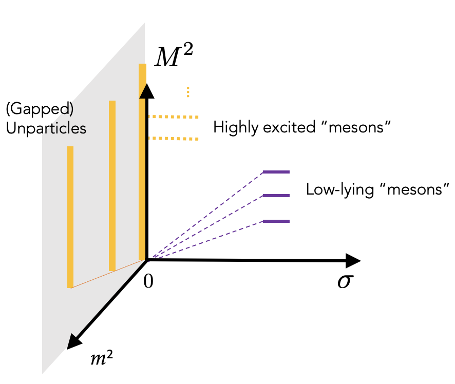
Figure 1: Schematic representation of the mass spectrum generated by the model defined by Eqs. (46) and (49). The behaviours of states with fixed $n$ (purple lines) and with fixed $\sigma n$ (dotted orange lines) are represented in the $m=0$ plane. The spectrum of gapped unparticles is represented in the $\sigma=0$ plane (solid orange lines).

Notice that the radial wave equation we derived in the present paper also appears from a bottom-up AdS/CFT perspective, see e.g. Afonin (2017). Interestingly, in the paper Argurio et al. (2016) where they consider a $U(1)$-invariant gauge theory in AdS₄ propagating a vector field and a complex scalar field, a nontrivial profile for the scalar field near the conformal infinity of AdS₄ introduces two dimensionful constants $m$ and $v$ that break conformal symmetry of the dual theory. Various limits where $m\rightarrow 0$ and $v\rightarrow 0$ relate a discrete spectrum with a massless Goldstone boson to a continuous Banks-Zaks-type spectrum for the scalar conformal operator in the dual CFT${}_{3}\,$. The approach of Argurio et al. (2016) enables a simultaneous discussion of spontaneous and dynamical symmetry breaking in a CFT at strong coupling. Some bridges may presumably be drawn between our model and the AdS/QCD framework, although it is out of the scope of the present paper. The interested reader may find a detailed discussions of mesons in AdS/QCD in the review Erdmenger et al. (2008).

One may finally wonder to what kind of gauge theory our toy model best applies. Similarities with $SU(2)$ QCD with one adjoint quark Athenodorou et al. (2015) have been commented in the text. However, our model is a priori better suited to model gauge theories with scalar matter than with fermionic matter, the variables $x_{i}(\tau)$ being then identified with two ”particles” of scalar matter. The existence of a conformal window is not limited to gauge theories with fermionic matter, as discussed in Appendix B. For example, a lattice study of $N_{f}=5$ scalar SU(2) Yang-Mills theory is affordable with current computers and could be performed to check the present model. We hope that such results will become available in the future.

Although we did not explicitly mention it, the present work and quoted references focus on zero-temperature gauge theories. The interplay between conformal window crossing and confinement/deconfinement transition may lead to new interesting phenomena, as discussed in Tuominen (2013). For example, a correspondence has been found between conformal QCD with $N_{f}=7$ and QCD with $N_{f}=2$ at $T\approx 2\,T_{c}$ ($T_{c}$ is the deconfinement temperature). To what extent the action (46) can be generalized at finite-temperature and bring relevant information is a problem that we leave for future works.

Appendix A The chain algorithm for gauge generators

We start from the constraint system (13)-(14) and seek for the generators of gauge transformations. According to the chain algorithm Castellani (1982) for the determination of the gauge generators, there is just one of them because we have only one primary first-class constraint. Also, the consistency algorithm stops after the secondary constraints: the desired generator consists in the sum of up to two terms. The constraint $\gamma_{1}$ itself cannot be a generator since $\{\gamma_{1},H_{T}\}$ is secondary. The generator is built with the first class constraints:

$$G=\dot{\varepsilon}(\tau)\gamma_{1}+\varepsilon(\tau)(a\gamma_{1}+b\gamma_{2})\;,$$ (56)

where $a$ and $b$ are arbitrary functions at this stage. Our goal is to fix these functions in order to give $G$ the properties of a generator of gauge transformation. Since the rules of the chain algorithm have to be respected, one imposes:

$$a\gamma_{1}+b\gamma_{2}+\{\gamma_{1},H_{T}\} =~{}~{}primary\;,$$ (57)

$$\{a\gamma_{1}+b\gamma_{2},H_{T}\} =~{}~{}primary\;.$$ (58)

The bracket $\{\gamma_{1},H_{T}\}=\gamma_{2}$ implies that $b$ must be equal to $-1\,$. Then, one knows that $\{\gamma_{2},H_{T}\}=\tilde{\lambda}_{2}\gamma_{2}\,$, thus one concludes that the other condition implies that $a$ must be equal to $\tilde{\lambda}_{2}$.
It can be then useful to notice the following relation:

$$\dot{e}_{1}=\{e_{1},H_{T}\} =\tilde{\lambda}_{2}e_{1}+C$$ (59)

$$\dot{e}_{2}=\{e_{2},H_{T}\} =\tilde{\lambda}_{2}e_{2}$$ (60)

$$\Rightarrow~{}\dot{e}_{1}\,\pi_{1}+\dot{e_{2}}\,\pi_{2}=C\,\pi_{1}+\tilde{\lambda}_{2}\,\gamma_{1}\;.$$ (61)

Thanks to this relation and recalling that $\gamma_{1}:=e_{1}\pi_{1}+e_{2}\pi_{2}\,$, one can rewrite $G=\dot{\varepsilon}\gamma_{1}+\varepsilon(\tilde{\lambda}_{2}\gamma_{1}-\gamma_{2})$ as follows:

$$G=\frac{d}{d\tau}(\varepsilon e_{1})\pi_{1}+\frac{d}{d\tau}(\varepsilon e_{2})\pi_{2}-(\varepsilon e_{1})\phi_{1}-(\varepsilon e_{2})\phi_{2}\;.$$ (62)

From this expression of the generator of gauge transformations, one reads off the transformations of the variables:

$$\delta e_{i}=\frac{d}{d\tau}(\varepsilon e_{i})\;,\qquad\delta x_{i}^{\mu}=\varepsilon\dot{x}^{\mu}_{i}\;.$$ (63)

These corresponds to the transformation formulae for reparametrization of the evolution parameter. It is direct to check that the action (3) is invariant under these transformations.

Appendix B Conformal window in gauge theories with scalar matter

The appearance of a conformal window in gauge theories with fermionic matter fields has been extensively discussed in Refs. Dietrich and Sannino (2007) and Sannino (2009) for the gauge groups $SU(N)$, $SO(2N)$ and $Sp(N)$. A similar but simpler analysis can be made for a Yang-Mills theory with scalar matter in the representation $R$ of the gauge algebra. The $\beta-$function of such a theory is given by $\beta(g)=\frac{g^{3}}{(4\pi)^{2}}\beta_{0}+\frac{g^{5}}{(4\pi)^{4}}\beta_{1}$, with $\beta_{0}=-\frac{11}{3}C_{2}({\rm adj})+\frac{N_{f}}{6}T(R)$, $\beta_{1}=-\frac{34}{3}C_{2}({\rm adj})^{2}+\frac{N_{f}}{3}\left(C_{2}({\rm adj})T(R)+6C_{2}(R)T(R)\right)$, where $C_{2}({\rm adj})$ and $C_{2}(R)$ are the quadratic Casimir operators in the adjoint and $R$ representations respectively, and where the index $T(R)$ is such that $C_{2}(R)\dim(R)=T(R)\dim({\rm adj})$ van Damme (1982).

Applying the methodology of Dietrich and Sannino (2007) but neglecting chiral symmetry issues, one may search for a conformal window in theories such that $\beta_{0}<0$ and $\beta_{1}>0$, i.e., with a number of flavours such that

$$\frac{34C_{2}({\rm adj})^{2}}{T(R)\left(C_{2}({\rm adj})+6C_{2}(R)\right)}<N_{f}<\frac{22C_{2}({\rm adj})}{T(R)},$$ (64)

the coupling constant $g^{*}$ at which it is observed being equal to $g^{*2}=-\frac{16\pi^{2}\beta_{0}}{\beta_{1}}$. The equation (64) admits nontrivial solutions. A simple example is the case of matter in adjoint representation, for which a conformal phase appears if $5<N_{f}<22$.

References

- Dietrich and Sannino (2007) Dietrich, D.D.; Sannino, F. Conformal window of SU(N) gauge theories with fermions in higher dimensional representations. Phys. Rev. 2007, D75, 085018, [arXiv:hep-ph/0611341].
- Di Pietro and Serone (2020) Di Pietro, L.; Serone, M. Looking through the QCD Conformal Window with Perturbation Theory. JHEP 2020, 07, 049, [arXiv:hep-th/2003.01742].
- Hasenfratz and Schaich (2018) Hasenfratz, A.; Schaich, D. Nonperturbative function of twelve-flavor SU(3) gauge theory. JHEP 2018, 02, 132, [arXiv:hep-lat/1610.10004].
- Hietanen et al. (2009) Hietanen, A.J.; Rantaharju, J.; Rummukainen, K.; Tuominen, K. Spectrum of SU(2) lattice gauge theory with two adjoint Dirac flavours. JHEP 2009, 05, 025, [arXiv:hep-lat/0812.1467].
- Del Debbio et al. (2016) Del Debbio, L.; Lucini, B.; Patella, A.; Pica, C.; Rago, A. Large volumes and spectroscopy of walking theories. Phys. Rev. D 2016, 93, 054505, [arXiv:hep-lat/1512.08242].
- Catterall and Sannino (2007) Catterall, S.; Sannino, F. Minimal walking on the lattice. Phys. Rev. D 2007, 76, 034504, [arXiv:hep-lat/0705.1664].
- Sannino (2009) Sannino, F. Conformal Windows of SP(2N) and SO(N) Gauge Theories. Phys. Rev. D 2009, 79, 096007, [arXiv:hep-ph/0902.3494].
- Neil (2011) Neil, E.T. Exploring Models for New Physics on the Lattice. PoS 2011, LATTICE2011, 009, [arXiv:hep-lat/1205.4706].
- Witzel (2019) Witzel, O. Review on Composite Higgs Models. PoS 2019, LATTICE2018, 006, [arXiv:hep-lat/1901.08216].
- Brower et al. (2019) Brower, R.C.; Hasenfratz, A.; Neil, E.T.; Catterall, S.; Fleming, G.; Giedt, J.; Rinaldi, E.; Schaich, D.; Weinberg, E.; Witzel, O. Lattice Gauge Theory for Physics Beyond the Standard Model. Eur. Phys. J. A 2019, 55, 198, [arXiv:hep-lat/1904.09964].
- Drach (2020) Drach, V. Composite electroweak sectors on the lattice. PoS 2020, LATTICE2019, 242, [arXiv:hep-lat/2005.01002].
- Cacciapaglia et al. (2020) Cacciapaglia, G.; Pica, C.; Sannino, F. Fundamental Composite Dynamics: A Review. Phys. Rept. 2020, 877, 1–70, [arXiv:hep-ph/2002.04914].
- Del Debbio et al. (2010) Del Debbio, L.; Patella, A.; Pica, C. Higher representations on the lattice: Numerical simulations. SU(2) with adjoint fermions. Phys. Rev. D 2010, 81, 094503, [arXiv:hep-lat/0805.2058].
- Casalbuoni and Gomis (2014) Casalbuoni, R.; Gomis, J. Conformal symmetry for relativistic point particles. Phys. Rev. 2014, D90, 026001, [arXiv:hep-th/1404.5766].
- Banks and Zaks (1982) Banks, T.; Zaks, A. On the Phase Structure of Vector-Like Gauge Theories with Massless Fermions. Nucl. Phys. B 1982, 196, 189–204.
- Georgi (2007) Georgi, H. Unparticle physics. Phys. Rev. Lett. 2007, 98, 221601, [hep-ph/0703260].
- Georgi and Kats (2008) Georgi, H.; Kats, Y. An Unparticle Example in 2D. Phys. Rev. Lett. 2008, 101, 131603, [arXiv:hep-ph/0805.3953].
- Ryttov and Sannino (2007) Ryttov, T.A.; Sannino, F. Conformal Windows of SU(N) Gauge Theories, Higher Dimensional Representations and The Size of The Unparticle World. Phys. Rev. D 2007, 76, 105004, [arXiv:hep-th/0707.3166].
- Casalbuoni and Gomis (2015) Casalbuoni, R.; Gomis, J. Conformal symmetry for relativistic point particles: an addendum. Phys. Rev. D 2015, 91, 047901, [arXiv:hep-th/1412.6903].
- Pramanik et al. (2014) Pramanik, S.; Ghosh, S.; Pal, P. Conformal Invariance in noncommutative geometry and mutually interacting Snyder Particles. Phys. Rev. D 2014, 90, 105027, [arXiv:hep-th/1409.0689].
- Henneaux (1992) Henneaux, M.; Teitelboim, C. Quantization of gauge systems. Princeton University Press: Princeton (N.J.), United States, 1992.
- Sazdjian (1988) Sazdjian, H. The massless bound state formalism in two particle relativistic quantum mechanics. Int. J. Mod. Phys. A 1988, 3, 1235–1261.
- Yáñez et al. (1994) Yáñez, R.J.; Van Assche, W.; Dehesa, J.S. Position and momentum information entropies of the D-dimensional harmonic oscillator and hydrogen atom. Phys. Rev. A 1994, 50, 3065–3079.
- Coon and Holstein (2002) Coon, S.A.; Holstein, B.R. Anomalies in Quantum Mechanics: the Potential. Am. J. Phys. 2002, 70, 513–519, [quant-ph/0202091].
- Krasnikov (2007) Krasnikov, N.V. Unparticle as a field with continuously distributed mass. Int. J. Mod. Phys. A 2007, 22, 5117–5120, [arXiv:hep-ph/0707.1419].
- Gaete and Spallucci (2008) Gaete, P.; Spallucci, E. A note on unparticle in lower dimensions. Phys. Lett. B 2008, 668, 336–339, [arXiv:hep-th/0807.0338].
- Nikolic (2008) Nikolic, H. Unparticle as a particle with arbitrary mass. Mod. Phys. Lett. A 2008, 23, 2645–2649, [arXiv:hep-ph/0801.4471].
- Deshpande and He (2008) Deshpande, N.G.; He, X.G. Unparticle Realization Through Continuous Mass Scale Invariant Theories. Phys. Rev. D 2008, 78, 055006, [arXiv:hep-ph/0806.2009].
- Delgado et al. (2007) Delgado, A.; Espinosa, J.R.; Quiros, M. Unparticles Higgs Interplay. JHEP 2007, 10, 094, [arXiv:hep-ph/0707.4309].
- Strassler (2008) Strassler, M.J. On the Phenomenology of Hidden Valleys with Heavy Flavor 2008. [arXiv:hep-ph/0806.2385].
- Megías and Quirós (2019) Megías, E.; Quirós, M. Gapped Continuum Kaluza-Klein spectrum. JHEP 2019, 08, 166, [arXiv:hep-ph/1905.07364].
- Braaten and Hammer (2021) Braaten, E.; Hammer, H.W. Neutral Charm Mesons near Threshold are Unparticles! 2021. [arXiv:hep-ph/2107.02831].
- Dubin et al. (1993) Dubin, A.Yu.; Kaidalov, A.B.; Simonov, Yu.A. The QCD string with quarks. 1. Spinless quarks. Phys. Atom. Nucl. 1993, 56, 1745–1759, [arXiv:hep-ph/hep-ph/9311344]. [Yad. Fiz.56,213(1993)].
- Buisseret (2007) Buisseret, F. Meson and glueball spectra with the relativistic flux tube model. Phys. Rev. 2007, C76, 025206, [arXiv:hep-ph/0705.0916].
- Sonnenschein and Weissman (2014) Sonnenschein, J.; Weissman, D. Rotating strings confronting PDG mesons. JHEP 2014, 08, 013, [arXiv:hep-ph/1402.5603].
- Chivukula (1997) Chivukula, R.S. A Comment on the zero temperature chiral phase transition in SU(N) gauge theories. Phys. Rev. 1997, D55, 5238–5240, [arXiv:hep-ph/hep-ph/9612267].
- Lucini (2015) Lucini, B. Numerical results for gauge theories near the conformal window. J. Phys. Conf. Ser. 2015, 631, 012065, [arXiv:hep-lat/1503.00371]. .
- Lombardo et al. (2014) Lombardo, M.P.; Miura, K.; Nunes da Silva, T.J.; Pallante, E. On the particle spectrum and the conformal window. JHEP 2014, 12, 183, [arXiv:hep-lat/1410.0298].
- Athenodorou et al. (2015) Athenodorou, A.; Bennett, E.; Bergner, G.; Lucini, B. Infrared regime of SU(2) with one adjoint Dirac flavor. Phys. Rev. D 2015, 91, 114508, [arXiv:hep-lat/1412.5994].
- Bergner et al. (2017) Bergner, G.; Giudice, P.; Münster, G.; Montvay, I.; Piemonte, S. Spectrum and mass anomalous dimension of SU(2) adjoint QCD with two Dirac flavors. Phys. Rev. D 2017, 96, 034504, [arXiv:hep-lat/1610.01576].
- Abramowitz and Stegun (1964) Abramowitz, M.; Stegun, I.A. Handbook of Mathematical Functions with Formulas, Graphs, and Mathematical Tables, ninth dover printing, tenth gpo printing ed.; Dover: New York, 1964.
- Tricomi and Erdelyi (1951) Tricomi, F.; Erdelyi, A. The asymptotic expansion of a ratio of gamma functions. Pacific J. Math. 1951, 1, 133–142.
- Stephanov (2007) Stephanov, M.A. Deconstruction of Unparticles. Phys. Rev. D 2007, 76, 035008, [arXiv:hep-ph/0705.3049].
- Afonin (2017) Afonin, S.S. Large degeneracy in light mesons from a modified soft-wall holographic model. Mod. Phys. Lett. A 2017, 32, 1750155, [arXiv:hep-ph/1708.08259].
- Argurio et al. (2016) Argurio, R.; Marzolla, A.; Mezzalira, A.; Musso, D. Analytic pseudo-Goldstone bosons. JHEP 2016, 03, 012, [arXiv:hep-th/1512.03750].
- Erdmenger et al. (2008) Erdmenger, J.; Evans, N.; Kirsch, I.; Threlfall, E. Mesons in Gauge/Gravity Duals - A Review. Eur. Phys. J. A 2008, 35, 81–133, [arXiv:hep-th/0711.4467].
- Tuominen (2013) Tuominen, K. Finite Temperature Phase Diagrams of Gauge Theories. Phys. Rev. D 2013, 87, 105014, [arXiv:hep-lat/1206.5772].
- van Damme (1982) van Damme, R.M.J. Most General Two Loop Counterterm for Fermion Free Gauge Theories With Scalar Fields. Phys. Lett. 1982, 110B, 239–241.
- Castellani (1982) Castellani, L. Symmetries in constrained Hamiltonian systems Annals of Physics 1982, 143, 357–371.