Quantum measurement with recycled photons

Abstract

We study a device composed of an optical interferometer integrated with a ferri-magnetic sphere resonator (FSR). Magneto-optic coupling can be employed in such a device to manipulate entanglement between optical pulses that are injected into the interferometer and the FSR. The device is designed to allow measuring the lifetime of such macroscopic entangled states in the region where environmental decoherence is negligibly small. This is achieved by recycling the photons interacting with the FSR in order to eliminate the entanglement before a pulse exits the interferometer. The proposed experiment may provide some insight on the quantum to classical transition associated with a measurement process.

I Introduction

Consider two successive quantum measurements Johansen_5760 . In the first one, which is performed at time $t_{1}$, the observable $A_{1}$ is being measured, whereas in the second one, which is performed at a later time $t_{2}\geq t_{1}$, the observable $A_{2}$ is being measured. Let $\mathcal{A}_{1}$ ($\mathcal{A}_{2}$) be the outcome of the first (second) measurement, and $\left\{a_{n,k}\right\}_{k}$ be the set of eigenvalues of the observable $A_{n}$, where $n\in\left\{1,2\right\}$. The probability that the measurement at time $t_{2}$ of the observable $A_{2}$ yields the value $a_{2,k_{2}}$, namely, the probability that $\mathcal{A}_{2}=a_{2,k_{2}}$, is denoted by $p_{2}\left(k_{2}\right)$ Two methods for the calculation of $p_{2}\left(k_{2}\right)$ are considered below. In the first one, the time evolution from an initial time $t_{0}<t_{1}$ to time $t_{2}$ is assumed to be purely unitary, and the probability $p_{2}\left(k_{2}\right)$ for the measurement at time $t_{2}$ is calculated using the Born rule. The second method is based on the assumption that the unitary evolution is disturbed at time $t_{1}$, at which the density operator of the system undergoes a collapse Schrodinger_807 ; Legget_R415 ; Aharonov_359 ; Mermin_38 ; Mooij_401 ; Bell_208 ; Zurek_1516 corresponding to the measurement of the observable $A_{1}$. Note that for both methods the coupling between the quantum subsystem and its measuring apparatus is taken into account in the unitary time evolution von_Neumann_Mathematical_Foundations ; Aharonov_11 ; Peres_book ; Braginsky_Quantum_Meas ; Ruskov_200404 . Under what conditions the probability $p_{2}\left(k_{2}\right)$ is affected Legget_857 by whether a collapse has occurred, or has not occurred, at the earlier time $t_{1}$?

A sufficient condition, which ensures that the collapse at time $t_{1}$ has no effect on the probability $p_{2}\left(k_{2}\right)$, is discussed below. This sufficient condition can be expressed as $\left[A_{2}\left(t_{2}\right),A_{1}\left(t_{1}\right)\right]=0$, where $A_{1}\left(t_{1}\right)$ and $A_{2}\left(t_{2}\right)$ are the Heisenberg representations of the $A_{1}$ and $A_{2}$ operators, respectively [see Eq. (8.501) of Buks_QMLN ]. As is explained below, this condition is satisfied for the vast majority of experimental setups used to study quantum systems.

Commonly the entire system can be composed into a quantum subsystem (QS) under study, and one or more ancilla subsystems (AS) that are used for probing the QS. Moreover, very commonly, the process of measurement is based on scattering of AS particles (electrons, photons, phonons, magnons, etc.) by the QS under study. In such a scattering process, the QS is bombarded by incoming AS particles. Properties of the QS are inferred from measured properties of the scattered AS particles. For this type of measurements the observables $A_{1}$ and $A_{2}$ are operators of the AS, and are independent on the degrees of freedom of the QS.

For the above-discussed two successive measurements of a given QS, two cases are considered below. For the first one, which is the common case, the ancilla particles that are used for the first measurement are not used for the second one. The two independent ASs associated with the two successive measurements are denoted by AS1 and AS2, respectively. For this case the observable $A_{1}$ ($A_{2}$) is an operator of AS1 (AS2), and consequently the condition $\left[A_{2}\left(t_{2}\right),A_{1}\left(t_{1}\right)\right]=0$ is satisfied, therefore, any collapse-induced effect on the probability $p_{2}\left(k_{2}\right)$ corresponding to the second measurement is excluded.

For the second case, AS particles used for performing the first measurement are recycled in order to participate in the second measurement as well. For this case, which is far less common, the condition $\left[A_{2}\left(t_{2}\right),A_{1}\left(t_{1}\right)\right]=0$ can be violated, and consequently collapse-induced effect on $p_{2}\left(k_{2}\right)$ cannot be ruled out. The possibility that the condition $\left[A_{2}\left(t_{2}\right),A_{1}\left(t_{1}\right)\right]=0$ is violated raises some concerns regarding the mathematical self-consistency of quantum mechanics Penrose_4864 ; Leggett_939 ; Leggett_022001 (note that this is unrelated to compatibility with the principle of causality).

II Optical interferometer

In the proposed experimental setup, a fiber optical loop mirror (FOLM) Mortimore_1217 ; Ibarra_191 is employed in order to allow performing measurements with recycled photons (see Fig. 1). A short optical pulse having state of polarization (SOP) $\left|p_{\mathrm{i}}\right\rangle$ is injected into port a1 of an optical coupler (OC). A Ferrimagnetic sphere resonator (FSR) kittel1976introduction ; Chai_1900252 is integrated into the fiber loop of the FOLM near port b1 of the OC. Magneto-optic (MO) coupling Freiser_152 ; Pershan_1482 between the optical pulse and the FSR gives rise to both the Faraday-Voigt effect, which accounts for the change in the optical SOP, and the inverse Faraday effect (IFE) Braggio_107205 ; Colautti_thesis ; Kirilyuk_2731 ; Kirilyuk_026501 ; Kimel_655 ; VanderZiel_190 ; Pershan_574 ; Hansteen_014421 ; Kirilyuk_748 , which accounts for the optically-induced change in the FSR state of magnetization (SOM). The externally injected optical pulse interacts with the FSR at times $t_{1}$, and $t_{2}>t_{1}$, and the experimental setup allows the violation of the condition $\left[A_{2}\left(t_{2}\right),A_{1}\left(t_{1}\right)\right]=0$, where $A_{1}\left(t_{1}\right)$ and $A_{2}\left(t_{2}\right)$ are the corresponding observables. The time difference $t_{2}-t_{1}$ is set by adjusting the length of the fiber loop (labelled as FOLM in Fig. 1). The transmitted signal at port a2 of the OC is measured using a photodetector (PD).

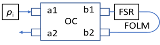
Figure 1: FOLM interferometer. Light is injected into port a1 of the OC, and detection is performed using a PD connected to port a2. The FSR is integrated inside a microwave cavity Mathai_054428 (not shown in the sketch).

The OC is characterized by forward (backward) transmission $t$ ($t^{\prime}$) and reflection $r$ ($r^{\prime}$) amplitudes. Incoming amplitudes $\bar{E}_{\mathrm{in}}=\left(\begin{array}[c]{cccc}E_{{}_{\rightarrow}}^{a_{1}}&E_{{}_{\rightarrow}}^{a_{2}}&E_{{}_{\leftarrow}}^{b_{1}}&E_{\leftarrow}^{b_{2}}\end{array}\right)^{\mathrm{T}}$ are related to outgoing amplitudes $\bar{E}_{\mathrm{out}}=\left(\begin{array}[c]{cccc}E_{{}_{\leftarrow}}^{a_{1}}&E_{{}_{\leftarrow}}^{a_{2}}&E_{{}_{\rightarrow}}^{b_{1}}&E_{\rightarrow}^{b_{2}}\end{array}\right)^{\mathrm{T}}$ by $\bar{E}_{\mathrm{out}}=S\bar{E}_{\mathrm{in}}$ (subscript horizontal arrow indicates propagation direction, and superscripts indicates OC port label), where the scattering matrix $S$ is given by (it is assumed that all scattering coefficients are polarization independent)

$$S=\left(\begin{array}[c]{cccc}0&0&t^{\prime}&r^{\prime}\\ 0&0&r^{\prime}&t^{\prime}\\ t&r&0&0\\ r&t&0&0\end{array}\right)\;.$$ (1)

Unitarity $S^{{\dagger}}S=1$ implies that $\left|t\right|^{2}+\left|r\right|^{2}=\left|t^{\prime}\right|^{2}+\left|r^{\prime}\right|^{2}=1$ and $\operatorname{Re}\left(r^{\ast}t\right)=\operatorname{Re}\left(r^{\prime\ast}t^{\prime}\right)=0$. Time reversal symmetry $S^{\mathrm{T}}=S$ implies that $t^{\prime}=t$ and $r^{\prime}=r=it\left|r/t\right|$.

The transmission (reflection) coefficient $t$ ($r$) is the amplitude of the sub-pulse circulating the FOLM in the clockwise (counter clockwise) direction. The MO coupling gives rise to a change in both the optical SOP and the FSR SOM. These states for the clockwise (counter clockwise) direction are labelled by $\left|p_{+}\right\rangle_{\mathrm{P}}$ and $\left|m_{+}\right\rangle_{\mathrm{M}}$ ($\left|p_{-}\right\rangle_{\mathrm{P}}$ and $\left|m_{-}\right\rangle_{\mathrm{M}}$), respectively (note that these states, which are allowed to change in time, are assumed to be normalized). The state vector $\left|\psi_{\mathrm{f}}\right\rangle$, which represents a final state after the pulse has left the interferometer, can be expressed as

$$\left|\psi_{\mathrm{f}}\right\rangle =tr^{\prime}\left|a_{1}\longleftarrow,p_{+},m_{+}\right\rangle+rt^{\prime}\left|a_{1}\longleftarrow,p_{-},m_{-}\right\rangle$$

$$+tt^{\prime}\left|a_{2}\longleftarrow,p_{+},m_{+}\right\rangle+rr^{\prime}\left|a_{2}\longleftarrow,p_{-},m_{-}\right\rangle\;,$$

(2)

where $\left|\mathrm{T},p,m\right\rangle=\left|\mathrm{T}\right\rangle_{\mathrm{I}}\otimes\left|p\right\rangle_{\mathrm{P}}\otimes\left|m\right\rangle_{\mathrm{M}}$ denotes a state having pulse in interferometer port $\mathrm{T}$, optical polarization $p$, and FSR magnetization $m$.

Let $\left\{\left|p_{n^{\prime}}\right\rangle_{\mathrm{P}}\right\}$ ($\left\{\left|m_{n^{\prime\prime}}\right\rangle_{\mathrm{M}}\right\}$) be an orthonormal basis for the Hilbert space of optical SOP (FSR SOM). The transmission $p_{\mathrm{T}}$ and reflection $p_{\mathrm{R}}$ probabilities are found by tracing out

$$p_{\mathrm{T}} =\sum_{n^{\prime},n^{\prime\prime}}\left|\left\langle\psi_{\mathrm{f}}\right|\left(\left|a_{2}\longleftarrow\right\rangle_{\mathrm{I}}\otimes\left|p_{n^{\prime}}\right\rangle_{\mathrm{P}}\otimes\left|m_{n^{\prime\prime}}\right\rangle_{\mathrm{M}}\right)\right|^{2}\;,$$ (3)

$$p_{\mathrm{R}} =\sum_{n^{\prime},n^{\prime\prime}}\left|\left\langle\psi_{\mathrm{f}}\right|\left(\left|a_{1}\longleftarrow\right\rangle_{\mathrm{I}}\otimes\left|p_{n^{\prime}}\right\rangle_{\mathrm{P}}\otimes\left|m_{n^{\prime\prime}}\right\rangle_{\mathrm{M}}\right)\right|^{2}\;,$$ (4)

hence (note that $\sum_{n^{\prime}}\left|p_{n^{\prime}}\right\rangle_{{}_{\mathrm{PP}}}\left\langle p_{n^{\prime}}\right|=1_{{}_{\mathrm{P}}}$, $\sum_{n^{\prime\prime}}\left|m_{n^{\prime\prime}}\right\rangle_{\mathrm{MM}}\left\langle m_{n^{\prime\prime}}\right|=1_{{}_{\mathrm{M}}}$, and recall that $\left|p_{\pm}\right\rangle_{\mathrm{P}}$ and $\left|m_{\pm}\right\rangle_{\mathrm{M}}$ are normalized, and that $t^{\prime}=t$ and $r^{\prime}=r=it\left|r/t\right|$)

$$p_{\mathrm{T}} =\left(\left|t\right|^{2}-\left|r\right|^{2}\right)^{2}+4\left|tr\right|^{2}\eta\;,$$ (5)

$$p_{\mathrm{R}} =4\left|tr\right|^{2}\left(1-\eta\right)\;,$$ (6)

where

$$\eta=\frac{1-\operatorname{Re}\left(\chi_{\mathrm{P}}\chi_{\mathrm{M}}\right)}{2}\;,$$ (7)

and where $\left.\chi_{\mathrm{P}}=\right._{\mathrm{P}}\left\langle p_{+}\right.\left|p_{-}\right\rangle_{\mathrm{P}}$ and $\left.\chi_{\mathrm{M}}=\right._{\mathrm{M}}\left\langle m_{+}\right.\left|m_{-}\right\rangle_{\mathrm{M}}$. Note that $p_{\mathrm{T}}+p_{\mathrm{R}}=1$ (recall that $\left|t\right|^{2}+\left|r\right|^{2}=1$). In the absence of any MO coupling, i.e. when $\chi_{\mathrm{P}}\chi_{\mathrm{M}}=1$, $\eta=0$, whereas $\eta=1/2$ for the opposite extreme case of $\chi_{\mathrm{P}}\chi_{\mathrm{M}}=0$. For the case of a 3dB OC (i.e. when $\left|t\right|^{2}=\left|r\right|^{2}=1/2$) this becomes $p_{\mathrm{T}}=\eta$ and $p_{\mathrm{R}}=1-\eta$. Thus, in the absence of any MO coupling and for a 3dB OC the transmission probability $p_{\mathrm{T}}$ vanishes. This unique property, which originates from destructive interference in the FOLM interferometer, allows sensitive measurement of the effect of MO coupling.

The parameter $\chi_{\mathrm{P}}$ characterizes the change in SOP induced by the Faraday-Voigt effect, whereas the change in the FSR SOM induced by the IFE Crescini_1 ; Braggio_107205 ; Hisatomi_174427 is characterized by the parameter $\chi_{\mathrm{M}}$. Both effects originate from the MO coupling between the optical pulses and the FSR, and the Verdet constant VanderZiel_190 ; Donati_372 ; Freiser_152 ; Pershan_1482 is proportional to both induced changes in SOP and SOM Battiato_014413 [see also Eq. (2.316) of Buks_WPLN ]. Based on appendix A, which reviews MO coupling, the parameter $\eta$ is estimated.

Two configurations are considered below. For the first one $\mathbf{\hat{q}}\parallel\mathbf{H}_{\mathrm{dc}}$, whereas $\mathbf{\hat{q}}\perp\mathbf{H}_{\mathrm{dc}}$ for the second configuration, where $\mathbf{\hat{q}}$ is a unit vector parallel to the optical propagation direction, and where $\mathbf{H}_{\mathrm{dc}}$ is the static magnetic field externally applied to the FSR. The angular frequency of the Kittel mode $\omega_{\mathrm{m}}$ is related to $H_{\mathrm{dc}}$ by $\omega_{\mathrm{m}}=\gamma_{\mathrm{e}}\mu_{0}H_{\mathrm{dc}}$, where $\gamma_{\mathrm{e}}/2\pi=28\operatorname{GHz}\operatorname{T}^{-1}$ is the gyromagnetic ratio, and $\mu_{0}$ is the free space permeability (magnetic anisotropy is disregarded). For both cases it is shown below that, on one hand, the intermediate value of $\operatorname{Re}\left(\chi_{\mathrm{P}}\chi_{\mathrm{M}}\right)$ during the time interval $\left[t_{1},t_{2}\right]$ can be made significantly smaller than unity, whereas, on the other hand, the final (i.e. after time $t_{2}$) value of $\operatorname{Re}\left(\chi_{\mathrm{P}}\chi_{\mathrm{M}}\right)$ can be made very close to unity [see Eq. (7)]. Hence, for these cases the transmitted signal at port a2 is strongly affected by the level of unitarity in the time evolution of the system prior to time $t_{2}$.

The change in SOP for the first configuration is dominated by the Faraday effect, whereas the Voigt effect, which is much weaker [see Eqs. (30), (31) and (34) of appendix A, and note that $Q_{\mathrm{s}}\ll 1$] accounts for the change in SOP for the second configuration. In the analysis below, the change in SOP is disregarded for the second configuration (i.e. it is assumed that $\chi_{\mathrm{P}}=1$).

The IFE gives rise to an effective magnetic field $\mathbf{H}_{\mathrm{IFE}}$, which is parallel to the optical propagation direction $\mathbf{\hat{q}}$, and it has a magnitude proportional to $I_{\mathrm{p+}}-I_{\mathrm{p-}}$, where $I_{\mathrm{p+}}$ ($I_{\mathrm{p-}}$) is the optical energy carried by right-hand $\left|R\right\rangle$ (left-hand $\left|L\right\rangle$) circular SOP VanderZiel_190 [see Eq. (40) of appendix A]. With femtosecond optical pulses this optically-induced magnetic field $\mathbf{H}_{\mathrm{IFE}}$ can be employed for ultrafast manipulation of the SOM Kimel_275 ; Juraschek_094407 ; Juraschek_043035 . For the first configuration (for which $\mathbf{\hat{q}}\parallel\mathbf{H}_{\mathrm{dc}}$), it is expected that the change in the SOM due to the IFE will be relatively small (since $\mathbf{H}_{\mathrm{IFE}}\parallel\mathbf{H}_{\mathrm{dc}}$, and the magnetization is assumed to be nearly parallel to $\mathbf{H}_{\mathrm{dc}}$). In the analysis below, the change in SOM is disregarded for the first configuration (i.e. it is assumed that $\chi_{\mathrm{M}}=1$). For the second configuration (for which $\mathbf{\hat{q}}\perp\mathbf{H}_{\mathrm{dc}}$), on the other hand, the IFE gives rise to a much larger effect (since $\mathbf{H}_{\mathrm{IFE}}$ is nearly perpendicular to the magnetization for this case).

III The case $\mathbf{\hat{q}}\parallel\mathbf{H}_{\mathrm{dc}}$

The Jones matrices corresponding to clockwise and counter-clockwise directions of loop circulation, are given by $J_{\mathrm{+}}=\sigma_{z}J_{\mathrm{S}}\left(t_{1}\right)$ and $J_{\mathrm{-}}=\sigma_{z}J_{\mathrm{S}}\left(t_{2}\right)\sigma_{z}\sigma_{z}$, respectively, where $J_{\mathrm{S}}\left(t\right)$ is the FSR Jones matrix at time $t$, and where $\bm{\sigma}=\left(\sigma_{x},\sigma_{y},\sigma_{z}\right)$ is the Pauli matrix vector [see Eq. (29) and Eqs. (14.106) and (14.112) of Buks_QMLN , and note that the transmission through the loop gives rise to a mirror reflection of the SOP and that $\sigma_{z}^{2}=1$]. The term $\chi_{\mathrm{P}}$ is thus given by $\chi_{\mathrm{P}}=\left\langle p_{\mathrm{i}}\right|J_{\mathrm{S}}^{{\dagger}}\left(t_{1}\right)J_{\mathrm{S}}\left(t_{2}\right)\left|p_{\mathrm{i}}\right\rangle$.

Let $\varphi_{\mathrm{S1}}$ and $\varphi_{\mathrm{S2}}$, be the rotation angles associated with the unitary transformations $J_{\mathrm{S}}\left(t_{1}\right)$ and $J_{\mathrm{S}}\left(t_{2}\right)$, respectively. For the case $\mathbf{\hat{q}}\parallel\mathbf{H}_{\mathrm{dc}}$, circular birefringence (CB) induced by the Faraday effect is the dominant mechanism giving rise to the change in SOP, and the corresponding Jones matrices $J_{\mathrm{S}}\left(t_{1}\right)$ and $J_{\mathrm{S}}\left(t_{2}\right)$ can be calculated using Eq. (34) with $\mathbf{k}_{\mathrm{B}}=\mathbf{k}_{\mathrm{CB}}$ [see Eq. (30)]. As is shown in appendix A, for the Faraday effect typically $\left|\varphi_{\mathrm{S1}}\right|\simeq 0.1$ and $\left|\varphi_{\mathrm{S2}}\right|\simeq 0.1$ for a magnetically saturated FSR of radius $R_{\mathrm{s}}\simeq 100\operatorname{\mu m}$. Hence, during the time interval $\left[t_{1},t_{2}\right]$, the intermediate value of $\operatorname{Re}\left(\chi_{\mathrm{P}}\right)$ is expected to be significantly smaller than unity.

The final (i.e. after time $t_{2}$) value of $\operatorname{Re}\left(\chi_{\mathrm{P}}\right)$ depends on the rotation angle $\varphi_{\mathrm{S}}$ associated with the unitary transformations $J_{\mathrm{S}}^{{\dagger}}\left(t_{1}\right)J_{\mathrm{S}}\left(t_{2}\right)$. The Jones matrix $J_{\mathrm{S}}$ given by Eq. (34) of appendix A is expressed as a function of the FSR SOM. For the case where FSR excitation during the time interval $\left(t_{1},t_{2}\right)$ is on the order of a single magnon, one has $\left|\varphi_{\mathrm{S}}\right|\simeq\left(l_{\mathrm{e}}/l_{\mathrm{P}}\right)\theta_{\mathrm{m0}}$, where $\theta_{\mathrm{m0}}$ is the magnetization rotation angle corresponding to a single magnon excitation. As is shown in appendix A, typically $l_{\mathrm{e}}/l_{\mathrm{P}}\simeq 10^{-1}$. From the Stoner–Wohlfarth energy $E_{\mathrm{M}}$ given by Eqs. (35) and (36) one finds that typically $\theta_{\mathrm{m0}}\simeq 10^{-9}$ (for the transition from the ground state to a single magnon excitation state). Hence the approximation $\chi_{\mathrm{P}}=1$ (i.e. $\varphi_{\mathrm{S}}=0$) can be safely employed in the calculation of $\eta$, provided that the the number of excited magnons is sufficiently small. The unique configuration of the proposed interferometer allows a finite value of $\operatorname{Re}\left(\chi_{\mathrm{P}}\right)$ very close to unity, in spite the fact that the intermediate value of $\operatorname{Re}\left(\chi_{\mathrm{P}}\right)$ can be significantly smaller than unity.

IV The case $\mathbf{\hat{q}}\perp\mathbf{H}_{\mathrm{dc}}$

For simplicity, consider first the case where the FSR is prepared in its ground state before the optical pulse is applied (i.e. initially the angle $\theta_{\mathrm{m}}$ between the magnetization and the externally applied static magnetic field $\mathbf{H}_{\mathrm{dc}}$ vanishes). Let $\theta_{\mathrm{IFE}}$ be the value of $\theta_{\mathrm{m}}$ immediately after the interaction with a pulse carrying a single optical photon. The intermediate value of $\operatorname{Re}\left(\chi_{\mathrm{M}}\right)$ during the time interval $\left[t_{1},t_{2}\right]$ is expected to be significantly smaller than unity provided that $\left|\theta_{\mathrm{IFE}}\right|\gtrsim\left|\theta_{\mathrm{m0}}\right|$ (recall that $\theta_{\mathrm{m0}}$ is the magnetization rotation angle corresponding to a single magnon excitation). This condition can be satisfied when angular momentum conversion between photons and magnons is sufficiently efficient Woodford_212412 . On the other hand, as is shown below, the final (i.e. after time $t_{2}$) value of $\operatorname{Re}\left(\chi_{\mathrm{M}}\right)$ can be made very close to unity. Note that the semiclassical model that is presented in appendix A allows expressing $\left|\theta_{\mathrm{m0}}\right|$ as a function of the magnetization tilt angle $\theta_{\mathrm{m}}$ and the constant $\theta_{\mathrm{mz}}$ given by Eq. (35) [see Eqs. (36) and (41)].

The level of entanglement associated with the state $\left|\psi_{\mathrm{f}}\right\rangle$ (2) can be characterized by the purity $\varrho_{\mathrm{i}}=\operatorname{Tr}\rho_{\mathrm{I}}^{2}=\operatorname{Tr}\rho_{\mathrm{M}}^{2}$ of the reduced density matrices $\rho_{\mathrm{I}}$ and $\rho_{\mathrm{M}}$ of the optical and FSR subsystems, respectively, which can be extracted from the Schmidt decomposition of $\left|\psi_{\mathrm{i}}\right\rangle$ Ekert_415 . In the absence of entanglement $\varrho_{\mathrm{i}}=1$, whereas for a maximized entanglement $\varrho_{\mathrm{i}}=1/2$. Consider the case of weak excitation, for which the SOM angle $\theta_{\mathrm{m}}$ is small. For this case, the Bosonization Holstein-Primakoff transformation Holstein_1098 can be employed, in order to allow the description of the state of the transverse magnetization in terms of a quantum state vector in the Hilbert space of a one-dimensional harmonic oscillator (i.e. a Boson). Such a description greatly simplifies the calculation of the purity $\varrho_{\mathrm{i}}$.

Consider the case where the SOP of the partial pulse hitting the FSR at time $t_{1}$ is adjusted to be circular left-hand $\left|L\right\rangle$ SOP. For that case the partial pulse hitting the FSR at the later time $t_{2}>t_{1}$ is expected to have circular right-hand $\left|R\right\rangle$ SOP (the loop gives rise to a mirror reflection of the SOP). The precession of the SOM with angular frequency $\omega_{\mathrm{m}}$ during the time interval $\left(t_{1},t_{2}\right)$ is described by the unitary time evolution operator $u\left(t_{2}-t_{1}\right)$, where $u\left(t\right)=\exp\left(-i\omega_{\mathrm{m}}ta_{\mathrm{m}}^{{\dagger}}a_{\mathrm{m}}\right)$, and where $a_{\mathrm{m}}$ is a magnon annihilation operator. The change in the SOM induced by the IFE due to the partial pulse hitting the FSR at time $t_{1}$ ($t_{2}$) is described by a displacement operator $D\left(\alpha_{\mathrm{i}}\right)$ ($D\left(-\alpha_{\mathrm{i}}\right)$), where the coherent state complex parameter $\alpha_{\mathrm{i}}$ has length given by $\left|\alpha_{\mathrm{i}}\right|=\theta_{\mathrm{IFE}}/\theta_{\mathrm{m0}}$. It is assumed that $\omega_{\mathrm{m}}t_{\mathrm{p}}\ll 1$, where $t_{\mathrm{p}}$ is the pulse time duration.

When the initial SOM is assumed to be a coherent state $\left|\alpha\right\rangle$ with a complex parameter $\alpha$, the final SOM corresponding to circulating the FOLM in the clockwise (counter clockwise) direction is a coherent state $\left|m_{+}\right\rangle_{\mathrm{M}}=\left|\alpha_{+}\right\rangle$ ($\left|m_{-}\right\rangle_{\mathrm{M}}=\left|\alpha_{-}\right\rangle$) with complex parameter $\alpha_{+}=\left(\alpha+\alpha_{\mathrm{i}}\right)e^{-i\omega_{\mathrm{m}}\left(t_{2}-t_{1}\right)}$ ($\alpha_{-}=\alpha e^{-i\omega_{\mathrm{m}}\left(t_{2}-t_{1}\right)}-\alpha_{\mathrm{i}}$) [see Eq. (5.53) of Buks_QMLN ]. The state vector $\left|\psi_{\mathrm{f}}\right\rangle$ can be expressed as $\left|\psi_{\mathrm{f}}\right\rangle=v_{1}\left|a_{1}\longleftarrow\right\rangle_{\mathrm{I}}\otimes\left|m_{1}\right\rangle_{\mathrm{M}}+v_{2}\left|a_{2}\longleftarrow\right\rangle_{\mathrm{I}}\otimes\left|m_{2}\right\rangle_{\mathrm{M}}$ , where $v_{1}=it^{2}\sqrt{\upsilon\nu_{+}}$, $\left|m_{1}\right\rangle_{\mathrm{M}}=\left(\left|\alpha_{+}\right\rangle+\left|\alpha_{-}\right\rangle\right)/\sqrt{\nu_{+}}$, $v_{2}=t^{2}\sqrt{\left(1-\upsilon\right)^{2}+\upsilon\nu_{-}}$, $\left|m_{2}\right\rangle_{\mathrm{M}}=\left(\left|\alpha_{+}\right\rangle-\upsilon\left|\alpha_{-}\right\rangle\right)/\sqrt{\left(1-\upsilon\right)^{2}+\upsilon\nu_{-}}$, $\mu=\left\langle\alpha_{+}\right.\left|\alpha_{-}\right\rangle=\mu^{\prime}+i\mu^{\prime\prime}$, with both $\mu^{\prime}$ and $\mu^{\prime\prime}$ being real, $\upsilon=\left|r/t\right|^{2}$ and $\nu_{\pm}=2\left(1\pm\mu^{\prime}\right)$ [see Eq. (2)]. Note that both $\left|m_{1}\right\rangle_{\mathrm{M}}$ and $\left|m_{2}\right\rangle_{\mathrm{M}}$ are normalized. The purity $\varrho_{\mathrm{i}}$ associated with the state $\left|\psi_{\mathrm{f}}\right\rangle$ is given by $\varrho_{\mathrm{i}}=1-2\left|v_{1}v_{2}\right|^{2}\left(1-\left|{}_{\mathrm{M}}\left\langle m_{1}\right.\left|m_{2}\right\rangle_{\mathrm{M}}\right|^{2}\right)$ [see Eq. (8.681) of Buks_QMLN ]. For a 3 dB OC, i.e. for $\upsilon=\left|r/t\right|^{2}=1$, this becomes $\varrho_{\mathrm{i}}=\left(1+\exp\left(-\left|\alpha_{+}-\alpha_{-}\right|^{2}\right)\right)/2$ [see Eq. (5.243) of Buks_QMLN ], or (note that $\varrho_{\mathrm{i}}$ is independent on $\alpha$)

$$\varrho_{\mathrm{i}}=\frac{1+\exp\left(-4\left|\alpha_{\mathrm{i}}\right|^{2}\cos^{2}\frac{\omega_{\mathrm{m}}\left(t_{2}-t_{1}\right)}{2}\right)}{2}\;.$$ (8)

The time interval $t_{2}-t_{1}$ can be set by adjusting the length of the fiber loop connecting ports b1 and b2 of the OC. A delay time of a single FSR period $\omega_{\mathrm{m}}/\left(2\pi\right)$ is obtained with fiber having length $L_{\mathrm{F}}$ given by $L_{\mathrm{F}}=cn_{\mathrm{F}}^{-1}\left(\omega_{\mathrm{m}}/\left(2\pi\right)\right)^{-1}=68\operatorname{mm}\left(n_{\mathrm{F}}/1.47\right)^{-1}\left(\left(\omega_{\mathrm{m}}/\left(2\pi\right)\right)/\left(3\operatorname{GHz}\right)\right)^{-1}$, where $n_{\mathrm{F}}$ is the fiber’s effective refractive index. When the ratio $\left(t_{2}-t_{1}\right)/\left(2\pi/\omega_{\mathrm{m}}\right)$ is much smaller than the FSR quality factor the effect of magnon damping can be disregarded.

During the time interval $\left(t_{1},t_{2}\right)$ the entanglement is nearly maximized provided that $e^{-\left|\alpha_{\mathrm{i}}\right|^{2}}\ll 1$. For a symmetric OC (i.e. for $\left|r/t\right|=1$), a full collapse accruing during this time interval results in a transmission probability $p_{\mathrm{T}}\simeq 1/2$, whereas unitary evolution yields $p_{\mathrm{T}}\simeq 0$. Consider the case where the condition $\cos\left(\omega_{\mathrm{m}}\left(t_{2}-t_{1}\right)/2\right)=0$ is satisfied. Note that for this case $u\left(t_{2}-t_{1}\right)\left|\alpha\right\rangle=\left|-\alpha\right\rangle$, hence the partial pulse hitting the FSR at time $t_{2}$ undoes the earlier change that has occurred at time $t_{1}$ (recall that the fiber loop gives rise to a mirror transformation $\left|L\right\rangle\rightarrow\left|R\right\rangle$ in the SOP), and consequently entanglement is eliminated, and the final state of the system $\left|\psi_{\mathrm{f}}\right\rangle$ after time $t_{2}$ becomes a product state, i.e. $\operatorname{Re}\left(\chi_{\mathrm{M}}\right)=1$

In the analysis above the Sagnac effect has been disregarded. In general, this effect, which gives rise to a relative phase shift between the clockwise and counter-clockwise partial pulses, can also contribute to the suppression of the destructive interference at the outgoing OC port a2. The Sagnac effect can be eliminated by placing the fiber loop in a plane parallel to the earth rotation axis.

V Summary

Devices similar to the one discussed here, which are based on ferrimagnetic MO coupling Almpanis_184406 ; Hisatomi_207401 ; Pantazopoulos_104425 ; Sharma_094412 ; Hisatomi_174427 , are currently being developed worldwide Lachance_070101 ; Wolski_2005_09250 ; Zhu_2005_06429 , mainly for the purpose of optically interfacing superconducting quantum circuits. Ultrafast (sub $\operatorname{ps}$ time scales) laser control of the SOM Kimel_275 can be employed for the preparation and manipulation of non-classical states of a FSR.

The device we propose here is designed to allow studying the quantum to classical transition associated with the interaction between an optical pulse and a FSR containing $\sim 10^{17}$ spins. The measured transmission probability $p_{\mathrm{T}}$ provides a very sensitive probe for non-unitarity in the system’s time evolution. Unitary evolution yields $p_{\mathrm{T}}\simeq 0$, whereas a full collapse occurring during the time interval $\left(t_{1},t_{2}\right)$ results in $p_{\mathrm{T}}\simeq 1/2$. The proposed experimental setup allows the generation of an entangled state during the time interval $\left(t_{1},t_{2}\right)$. The level of entanglement after time $t_{2}$ can be controlled by adjusting the time duration $t_{1}-t_{2}$ (which can be made much shorter than all time scales characterizing environmental decoherence). Systematic measurements of the transmission probability $p_{\mathrm{T}}$ with varying parameters may provide an important insight on the non-unitary nature of a quantum measurement.

VI Acknowledgments

This work was supported by the Israeli science foundation, the Israeli ministry of science, and by the Technion security research foundation.

Appendix A Magneto-optics

In this appendix the MO Faraday, Voigt and inverse Faraday effects are briefly reviewed.

A.1 Macroscopic Maxwell’s equations

In the absent of current sources, the macroscopic Maxwell’s equations in Fourier space are given by

$$i\mathbf{q}\times\mathbf{H}_{\mathrm{T}}\left(\mathbf{q},\omega\right) =-\frac{i\omega}{c}\mathbf{D}\left(\mathbf{q},\omega\right)\;,$$ (9)

$$\mathbf{q}\times\mathbf{E}_{\mathrm{T}}\left(\mathbf{q},\omega\right) =\frac{\omega}{c}\mathbf{B}\left(\mathbf{q},\omega\right)\;,$$ (10)

$$i\mathbf{q}\cdot\mathbf{D}_{\mathrm{L}}\left(\mathbf{q},\omega\right) =4\pi\rho_{\mathrm{ext}}\left(\mathbf{q},\omega\right)\;,$$ (11)

$$\mathbf{q}\cdot\mathbf{B}_{\mathrm{L}}\left(\mathbf{q},\omega\right) =0\;,$$ (12)

where $\mathbf{H}$ is the magnetic field, $\mathbf{E}$ is the electric field, $\mathbf{B}$ is the magnetic induction, $\mathbf{D}$ is the electric displacement, $\rho_{\mathrm{ext}}$ is the charge density, $c$ is the speed of light, $\mathbf{q}$ is the Fourier wave vector, and $\omega$ is the Fourier angular frequency. All vector fields $\mathbf{F}\in\left\{\mathbf{H},\mathbf{E},\mathbf{B},\mathbf{D}\right\}$ are decomposed into longitudinal and transverse parts with respect to the wave vector $\mathbf{q}$ according to $\mathbf{F}=\mathbf{F}_{\mathrm{L}}+\mathbf{F}_{\mathrm{T}}$. where the longitudinal part is given by $\mathbf{F}_{\mathrm{L}}=\left(\mathbf{\hat{q}}\cdot\mathbf{F}\right)\mathbf{\hat{q}}$, the transverse one is given by $\mathbf{F}_{\mathrm{T}}=\left(\mathbf{\hat{q}}\times\mathbf{F}\right)\times\mathbf{\hat{q}}$, and where $\mathbf{\hat{q}}=\mathbf{q/}\left|\mathbf{q}\right|$ is a unit vector in the direction of $\mathbf{q}$. For an isotropic and linear medium the following relations hold $\mathbf{D}=\epsilon_{\mathrm{m}}\mathbf{E}$, where $\epsilon_{\mathrm{m}}$ is the permittivity tensor, and $\mathbf{B}=\mu_{\mathrm{m}}\mathbf{H}$, where $\mu_{\mathrm{m}}$ is the permeability tensor. In the optical band to a good approximation $\mu_{\mathrm{m}}$ is the identity tensor.

By applying $\mathbf{q}\times$ to Eq. (10) from the left, and employing Eq. (9) one obtains $\mathbf{q}\times\left(\mathbf{q}\times\mathbf{E}_{\mathrm{T}}\right)=-\epsilon\left(\omega/c\right)^{2}\mathbf{E}_{\mathrm{T}}$ Freiser_152 ; Boardman_197 ; Boardman_388 , or in a matrix form [note that for general vectors $\mathbf{u}$ and $\mathbf{v}$ the following holds $\mathbf{u}\times\left(\mathbf{u}\times\mathbf{v}\right)=\left(\mathbf{uu}^{\mathrm{T}}-\mathbf{u}\cdot\mathbf{u}\right)\mathbf{v}$]

$$\left(M_{\epsilon}+1-\frac{n^{2}}{n_{0}^{2}}\right)\mathbf{E}_{\mathrm{T}}=0\;,$$ (13)

where the $3\times 3$ matrix $M_{\epsilon}$ is given by

$$M_{\epsilon}=\frac{\epsilon_{\mathrm{m}}}{n_{0}^{2}}+\frac{\mathbf{qq}^{\mathrm{T}}}{n_{0}^{2}q_{0}^{2}}-1=\frac{\epsilon_{\mathrm{m}}+n^{2}P_{\mathbf{\hat{q}}}}{n_{0}^{2}}-1\;,$$ (14)

$\mathbf{q}=q\mathbf{\hat{q}}$, $\mathbf{\hat{q}}=\left(\sin\theta\cos\phi,\sin\theta\sin\phi,\cos\theta\right)$, $q_{0}=\omega/c$, $n_{0}$ is the medium refractive index, $n=q/q_{0}$, and where $P_{\mathbf{\hat{u}}}=\mathbf{\hat{u}\hat{u}}^{\mathrm{T}}$ is a projection matrix associated with a given unit vector $\mathbf{\hat{u}}$ (the $3\times 3$ identity matrix is denoted by $1$). Note that $n^{2}/n_{0}^{2}-1\simeq 2\left(n-n_{0}\right)/n_{0}$ provided that $\left|n-n_{0}\right|\ll n_{0}$.

For a ferromagnet or a ferrimagnet medium, it is assumed that the elements $\epsilon_{ij}$ are functions of the magnetization vector $\mathbf{M}$. The Onsager’s time-reversal symmetry relation reads $\epsilon_{ij}\left(\mathbf{M}\right)=\epsilon_{ji}\left(-\mathbf{M}\right)$. Moreover, it is expected that $\epsilon_{ij}\left(\mathbf{M}=0\right)=0$ for $i\neq j$. The static magnetic field $\mathbf{H}_{\mathrm{dc}}$ is assumed to be parallel to the $\mathbf{\hat{z}}$ direction. For the case where $\mathbf{M}$ is parallel to $\mathbf{H}_{\mathrm{dc}}$ (i.e. parallel to $\mathbf{\hat{z}}$) the tensor $\epsilon_{\mathrm{m}}$ is assumed to have the form Boardman_197 ; Boardman_388

$$\frac{\epsilon_{\mathrm{m}}}{n_{0}^{2}}=1+iQM_{\mathrm{C}}\;,$$ (15)

where the matrix $M_{\mathrm{C}}$ is given by

$$M_{\mathrm{C}}=\left(\begin{array}[c]{ccc}0&-1&0\\ 1&0&0\\ 0&0&0\end{array}\right)\;.$$ (16)

The value of $Q$ corresponding to saturated magnetization is denoted by $Q_{\mathrm{s}}$. For YIG $Q_{\mathrm{s}}\simeq 10^{-4}$ for (free space) wavelength $\lambda_{0}\simeq 1550\operatorname{nm}$ in the telecom band Wood_1038 . The corresponding polarization beat length $l_{\mathrm{P}}$ is given by $l_{\mathrm{P}}=\lambda_{0}/\left(n_{0}Q_{\mathrm{s}}\right)\simeq 7.\,0\operatorname{mm}$, where $n_{0}=2.19$ is the refractive index of YIG in the telecom band. In this band $l_{\mathrm{P}}/l_{\mathrm{A}}\simeq 0.014\,$, where $l_{\mathrm{A}}^{-1}=\left(0.5\operatorname{m}\right)^{-1}$ is the YIG absorption coefficient Zhang_591 ; Onbasli_1 ; Donati_372 ; Jooss_651 .

To analyze the change in the SOP induced by MO coupling, a rotation transformation is applied to a coordinate system having a $z$ axis parallel to the propagation direction ($\mathbf{\hat{q}}$ in the non-rotated frame). Let $M_{\epsilon}^{\prime}$ be the transformed matrix that represents the matrix $M_{\epsilon}$ in that coordinate system. For a given unit vector $\mathbf{\hat{u}}$, the rotation matrix $R_{\mathbf{\hat{u}}}$ is defined by the relation $R_{\mathbf{\hat{u}}}\mathbf{\hat{u}}=\mathbf{\hat{z}}$. The unit vector parallel to the magnetization $\mathbf{M}$ is denoted by $\mathbf{\hat{m}}=\left(\sin\theta_{\mathrm{m}}\cos\phi_{\mathrm{m}},\sin\theta_{\mathrm{m}}\sin\phi_{\mathrm{m}},\cos\theta_{\mathrm{m}}\right)$. The transformed matrix $M_{\epsilon}^{\prime}$ is given by

$$M_{\epsilon}^{\prime}=\frac{R_{\mathbf{\hat{q}}}R_{\mathbf{\hat{m}}}^{-1}\epsilon_{\mathrm{m}}R_{\mathbf{\hat{m}}}R_{\mathbf{\hat{q}}}^{-1}+n^{2}P_{\mathbf{\hat{z}}}}{n_{0}^{2}}-1\;.$$ (17)

Note that Eq. (17) implies that (note that $R_{\mathbf{\hat{q}}}^{-1}\mathbf{\hat{z}}=\mathbf{\hat{q}}$ and $R_{\mathbf{\hat{u}}}^{-1}=R_{\mathbf{\hat{u}}}^{\mathrm{T}}$)

$$R_{\mathbf{\hat{q}}}^{-1}M_{\epsilon}^{\prime}R_{\mathbf{\hat{q}}}=\frac{R_{\mathbf{\hat{m}}}^{-1}\epsilon_{\mathrm{m}}R_{\mathbf{\hat{m}}}+n^{2}P_{\mathbf{\hat{q}}}}{n_{0}^{2}}-1\;,$$ (18)

and

$$R_{\mathbf{\hat{m}}}R_{\mathbf{\hat{q}}}^{-1}M_{\epsilon}^{\prime}R_{\mathbf{\hat{q}}}R_{\mathbf{\hat{m}}}^{-1}=\frac{\epsilon_{\mathrm{m}}+n^{2}R_{\mathbf{\hat{m}}}P_{\mathbf{\hat{q}}}R_{\mathbf{\hat{m}}}^{-1}}{n_{0}^{2}}-1\;.$$ (19)

Note also that [see Eq. (6.235) of Buks_QMLN ]

$$\frac{R_{\mathbf{\hat{m}}}^{-1}\left(\frac{\epsilon_{\mathrm{m}}}{n_{0}^{2}}-1\right)R_{\mathbf{\hat{m}}}}{iQ_{\mathrm{s}}}=R_{\mathbf{\hat{m}}}^{-1}M_{\mathrm{C}}R_{\mathbf{\hat{m}}}=C_{\mathbf{\hat{m}}}\;,$$ (20)

where the matrix $C_{\mathbf{\hat{u}}}$, which is defined by

$$C_{\mathbf{\hat{u}}}=\left(\begin{array}[c]{ccc}0&-\mathbf{\hat{u}}\cdot\mathbf{\hat{z}}&\mathbf{\hat{u}}\cdot\mathbf{\hat{y}}\\ \mathbf{\hat{u}}\cdot\mathbf{\hat{z}}&0&-\mathbf{\hat{u}}\cdot\mathbf{\hat{x}}\\ -\mathbf{\hat{u}}\cdot\mathbf{\hat{y}}&\mathbf{\hat{u}}\cdot\mathbf{\hat{x}}&0\end{array}\right)\;,$$ (21)

is the cross-product matrix corresponding to a given unit vector $\mathbf{\hat{u}}$, and for an arbitrary 3-dimensional vector $\mathbf{v}$ the following holds $\mathbf{\hat{u}\times v=}C_{\mathbf{\hat{u}}}\mathbf{v}$ [see Eq. (6.243) of Buks_QMLN ]. The following holds

$$C_{\mathbf{\hat{m}}}=M_{\mathrm{C}}+M_{\perp}+O\left(\theta_{\mathrm{m}}^{2}\right)\;,$$ (22)

where the matrix $M_{\perp}$ is given by

$$M_{\perp}=\theta_{\mathrm{m}}\left(\begin{array}[c]{ccc}0&0&\sin\phi_{\mathrm{m}}\\ 0&0&-\cos\phi_{\mathrm{m}}\\ -\sin\phi_{\mathrm{m}}&\cos\phi_{\mathrm{m}}&0\end{array}\right)\;,$$ (23)

hence to first order in $\theta_{\mathrm{m}}$ one has [see Eq. (17), and note that the approximation $\left(n^{2}/n_{0}^{2}\right)P_{\mathbf{\hat{z}}}\simeq P_{\mathbf{\hat{z}}}$ is being employed]

$$M_{\epsilon}^{\prime}=iQ_{\mathrm{s}}R_{\mathbf{\hat{q}}}\left(M_{\mathrm{C}}+M_{\perp}\right)R_{\mathbf{\hat{q}}}^{-1}+P_{\mathbf{\hat{z}}}\;,$$ (24)

or [compare with Eq. (20)]

$$M_{\epsilon}^{\prime}=\left(\begin{array}[c]{ccc}0&-iQ_{z}&-iQ_{y}\\ iQ_{z}&0&iQ_{x}\\ iQ_{y}&-iQ_{x}&1\end{array}\right)+iQ_{\mathrm{s}}R_{\mathbf{\hat{q}}}M_{\perp}R_{\mathbf{\hat{q}}}^{-1}\;,$$ (25)

where $\left(Q_{x},Q_{y},Q_{z}\right)=Q_{\mathrm{s}}\mathbf{\hat{q}}$.

An effective $2\times 2$ matrix $M_{\mathrm{T}}$ corresponding to the transverse components of the electric field (spanned by the first two vectors) is evaluated below using Eq. (4.87) of Buks_QMLN .  When terms of orders $\theta_{\mathrm{m}}Q_{\mathrm{s}}^{2}$ are disregarded (it is assumed that $\left|\theta_{\mathrm{m}}\right|\ll 1$ and $Q_{\mathrm{s}}\ll 1$), one finds using the relation

$$\frac{\left(\begin{array}[c]{ccc}1&0&0\\ 0&1&0\\ 0&0&0\end{array}\right)R_{\mathbf{\hat{q}}}M_{\perp}R_{\mathbf{\hat{q}}}^{-1}\left(\begin{array}[c]{ccc}1&0&0\\ 0&1&0\\ 0&0&0\end{array}\right)}{\theta_{\mathrm{m}}\cos\left(\phi-\phi_{\mathrm{m}}\right)\sin\theta}=M_{\mathrm{C}}\;,$$ (26)

that

$$M_{\mathrm{T}}=Q_{\mathrm{s}}\alpha_{\mathrm{CB}}\left(\begin{array}[c]{cc}0&-i\\ i&0\end{array}\right)+\left(\begin{array}[c]{cc}-Q_{y}^{2}&Q_{x}Q_{y}\\ Q_{x}Q_{y}&-Q_{x}^{2}\end{array}\right)\;,$$

where $\alpha_{\mathrm{CB}}$ is given by [recall that $\cos\left(\phi-\phi_{\mathrm{m}}\right)=\cos\phi\cos\phi_{\mathrm{m}}+\sin\phi\sin\phi_{\mathrm{m}}$]

$$\alpha_{\mathrm{CB}}=\frac{Q_{z}}{Q_{\mathrm{s}}}+\theta_{\mathrm{m}}\cos\left(\phi-\phi_{\mathrm{m}}\right)\sin\theta=\mathbf{\hat{q}}\cdot\mathbf{\hat{m}}+O\left(\theta_{\mathrm{m}}^{2}\right)\;,$$ (27)

or

$$M_{\mathrm{T}}=k_{0}\sigma_{0}+\mathbf{k}_{\mathrm{B}}\cdot\mathbf{\sigma}\;,$$ (28)

where $k_{0}=-\left(Q_{x}^{2}+Q_{y}^{2}\right)/2$, $\sigma_{0}$ is the $2\times 2$ identity matrix, the Pauli matrix vector $\bm{\sigma}=\left(\sigma_{x},\sigma_{y},\sigma_{z}\right)$ is given by

$$\sigma_{x}=\left(\begin{array}[c]{cc}0&1\\ 1&0\end{array}\right),\;\sigma_{y}=\left(\begin{array}[c]{cc}0&-i\\ i&0\end{array}\right),\;\sigma_{z}=\left(\begin{array}[c]{cc}1&0\\ 0&-1\end{array}\right)\;,$$ (29)

the birefringence vector $\mathbf{k}_{\mathrm{B}}$ is expressed as $\mathbf{k}_{\mathrm{B}}=\mathbf{k}_{\mathrm{CB}}+\mathbf{k}_{\mathrm{LB}}$, with (to first order in $\theta_{\mathrm{m}}$)

$$\mathbf{k}_{\mathrm{CB}}=Q_{\mathrm{s}}\left(0,\mathbf{\hat{q}}\cdot\mathbf{\hat{m}},0\right)\;,$$ (30)

and

$$\mathbf{k}_{\mathrm{LB}}=Q_{\mathrm{s}}^{2}\left(S\left(-\frac{\pi}{4}\right),0,S\left(\frac{\pi}{4}\right)\right)\;,$$ (31)

where the squeezing transformation $S\left(\varrho\right)$ is given by

$$S\left(\varrho\right)=\frac{e^{i\left(\varrho-\frac{\pi}{4}\right)}\mathcal{Q}^{2}+e^{-i\left(\varrho-\frac{\pi}{4}\right)}\mathcal{Q}^{\ast 2}}{4}\;,$$ (32)

and where $\mathcal{Q}=\left(Q_{x}+iQ_{y}\right)/Q_{\mathrm{s}}$.

A.2 Jones matrices

In general, the transformation between input SOP and output SOP for a given optical element can be described using a Jones matrix $J$ Potton_717 . For the loss-less case the matrix $J$ is unitary, and it can be expressed as $J=B\left(\mathbf{\hat{u}},\varphi\right)$, where

$$B\left(\mathbf{\hat{u}},\varphi\right)\dot{=}\exp\left(-\frac{i\mathbf{\sigma}\cdot\mathbf{\hat{u}}\varphi}{2}\right)=\mathbf{1}\cos\frac{\varphi}{2}-i\mathbf{\sigma}\cdot\mathbf{\hat{u}}\sin\frac{\varphi}{2}\;,$$ (33)

and where $\mathbf{\hat{u}}$ is a unit vector and $\varphi$ is a rotation angle. The colinear vertical, horizontal, diagonal and anti-diagonal SOP are denoted by $\left|V\right\rangle$, $\left|H\right\rangle$, $\left|D\right\rangle=2^{-1/2}\left(\left|H\right\rangle+\left|V\right\rangle\right)$ and $\left|A\right\rangle=2^{-1/2}\left(\left|H\right\rangle-\left|V\right\rangle\right)$ , respectively, whereas the circular right-hand and left-hand SOP are denoted by $\left|R\right\rangle=2^{-1/2}\left(\left|H\right\rangle-i\left|V\right\rangle\right)$ and $\left|L\right\rangle=2^{-1/2}\left(\left|H\right\rangle+i\left|V\right\rangle\right)$ , respectively. The unit vectors in the Poincaré sphere corresponding to the SOP $\left|V\right\rangle$, $\left|H\right\rangle$, $\left|D\right\rangle$, $\left|A\right\rangle$, $\left|R\right\rangle$ and $\left|L\right\rangle$, are $\mathbf{\hat{z}}$, $-\mathbf{\hat{z}}$, $\mathbf{\hat{x}}$, $-\mathbf{\hat{x}}$, $-\mathbf{\hat{y}}$ and $\mathbf{\hat{y}}$, respectively.

Consider a FSR having radius $R_{\mathrm{s}}$ and saturated magnetization. When damping is disregarded the sphere’s Jones matrix $J_{\mathrm{S}}$ is given by [see Eqs. (28) and (33)]

$$J_{\mathrm{S}}=B\left(\frac{\mathbf{k}_{\mathrm{B}}}{\left|\mathbf{k}_{\mathrm{B}}\right|},\frac{l_{\mathrm{e}}}{l_{\mathrm{P}}}\frac{\left|\mathbf{k}_{\mathrm{B}}\right|}{Q_{\mathrm{s}}}\right)\;,$$ (34)

where $l_{\mathrm{e}}\simeq 2R_{\mathrm{s}}$ is the effective optical travel length inside the sphere. The first order in $Q_{\mathrm{s}}$ component of $\mathbf{k}_{\mathrm{B}}=\mathbf{k}_{\mathrm{CB}}+\mathbf{k}_{\mathrm{LB}}$ in the $y$ direction [see Eq. (30)] gives rise to CB known as the Faraday effect, whereas the second order in $Q_{\mathrm{s}}$ components in the $xz$ plane give rise to colinear birefringence (LB) known as the Voigt (Cotton-Mouton) effect [see Eq. (31)]. The eigenvectors corresponding to CB (LB) have circular (colinear) polarization.

A.3 Stoner–Wohlfarth energy

When anisotropy is disregarded, the Stoner–Wohlfarth energy $E_{\mathrm{M}}$ of the FSR is given by $E_{\mathrm{M}}=-\mu_{0}V_{\mathrm{s}}M_{\mathrm{s}}H_{\mathrm{dc}}\cos\theta_{\mathrm{m}}$, where $\mu_{0}$ is the free space permeability, $V_{\mathrm{s}}=4\pi R_{\mathrm{s}}^{3}/3$ is the volume of the sphere having radius $R_{\mathrm{s}}$, $M_{\mathrm{s}}$ is the saturation magnetization ($M_{\mathrm{s}}=140\operatorname{kA}/\operatorname{m}$ for YIG at room temperature), $H_{\mathrm{dc}}$ is the static magnetic field, which is related to the angular frequency of the Kittel mode $\omega_{\mathrm{m}}$ by $H_{\mathrm{dc}}=\omega_{\mathrm{m}}/\left(\mu_{0}\gamma_{\mathrm{e}}\right)$ Fletcher_687 ; sharma2019cavity , and $\theta_{\mathrm{m}}$ is the angle between the magnetization and static magnetic field vectors Stancil_Spin . In terms of the angle $\theta_{\mathrm{mz}}$, which is given by

$$\theta_{\mathrm{mz}}=\frac{2\hbar\gamma_{\mathrm{e}}}{V_{\mathrm{s}}M_{\mathrm{s}}}=\frac{3.2\times 10^{-17}}{\left(\frac{R_{\mathrm{s}}}{125\operatorname{\mu m}}\right)^{3}\frac{M_{\mathrm{s}}}{140\operatorname{kA}/\operatorname{m}}}\;,$$ (35)

the energy $E_{\mathrm{M}}$ can be expressed as

$$E_{\mathrm{M}}=-2\hbar\omega_{\mathrm{m}}\frac{\cos\theta_{\mathrm{m}}}{\theta_{\mathrm{mz}}}\;.$$ (36)

A.4 IFE effective magnetic field

Consider the case where the second order in $Q_{\mathrm{s}}$ LB induced by the Voigt effect can be disregarded. For this case, for which $\mathbf{k}_{\mathrm{B}}$ becomes parallel to the $\mathbf{\hat{y}}$ direction in the Poincaré space, it is convenient to express the transverse electric field in the basis of circular SOP $\mathbf{E}_{\mathrm{T}}^{\prime}=E_{+}\mathbf{\hat{u}}_{+}+E_{-}\mathbf{\hat{u}}_{-}$, where $\mathbf{\hat{u}}_{\pm}=\left(e^{\mp i\pi/4}/\sqrt{2},e^{\pm i\pi/4}/\sqrt{2}\right)^{\mathrm{T}}$ (note that $\sigma_{y}\mathbf{\hat{u}}_{\pm}=\pm\mathbf{\hat{u}}_{\pm}$). For this case the electric energy density $u_{\mathrm{E}}=\left(\epsilon_{0}/2\right)\left(\mathbf{E}_{\mathrm{T}}^{\prime{\dagger}}\epsilon_{\mathrm{m}}^{\prime}\mathbf{E}_{\mathrm{T}}^{\prime}\right)$ can be expressed as [see Eqs. (17), (28) and (30)]

$$u_{\mathrm{E}}=\epsilon_{0}\frac{n_{+}^{2}\left|E_{+}\right|^{2}+n_{-}^{2}\left|E_{-}\right|^{2}}{2}\;,$$ (37)

where $\left|E_{+}\right|^{2}$ ($\left|E_{-}\right|^{2}$) is proportional to the intensity of right-hand $\left|R\right\rangle$ (left-hand $\left|L\right\rangle$) circular SOP, $n_{\pm}=n_{0}\left(1\pm\left|\mathbf{k}_{\mathrm{CB}}\right|\right)^{1/2}$, and $\left|\mathbf{k}_{\mathrm{CB}}\right|=Q_{\mathrm{s}}\left|\mathbf{\hat{q}}\cdot\mathbf{\hat{m}}\right|$. Alternatively, $u_{\mathrm{E}}\$can be expressed as $u_{\mathrm{E}}=u_{\mathrm{E0}}+u_{\mathrm{E1}}$, where $u_{\mathrm{E0}}=\left(\epsilon_{0}n_{0}^{2}/2\right)\left(\left|E_{+}\right|^{2}+\left|E_{-}\right|^{2}\right)$ and $u_{\mathrm{E1}}=\left(\epsilon_{0}n_{0}^{2}\left|\mathbf{k}_{\mathrm{CB}}\right|/2\right)\left(\left|E_{+}\right|^{2}-\left|E_{-}\right|^{2}\right)$. When the energy density is uniformly distributed inside the FSR, the energy $U_{\mathrm{T}}=V_{\mathrm{s}}u_{\mathrm{E1}}$ is given by $U_{\mathrm{T}}=\hbar\omega_{\mathrm{e}}\left|\mathbf{k}_{\mathrm{CB}}\right|=\hbar\omega_{\mathrm{e}}Q_{\mathrm{s}}\left(\mathbf{\hat{q}}\cdot\mathbf{\hat{m}}\right)$ [see Eq. (30)] where

$$\omega_{\mathrm{e}}=\frac{\epsilon_{0}n_{0}^{2}V_{\mathrm{s}}\left(\left|E_{+}\right|^{2}-\left|E_{-}\right|^{2}\right)}{2\hbar}\;,$$ (38)

or

$$U_{\mathrm{T}}=\frac{\mu_{0}}{2}\mathbf{H}_{\mathrm{IFE}}\cdot\mathbf{M}\;,$$ (39)

where the IFE effective magnetic field $\mathbf{H}_{\mathrm{IFE}}$ is given by

$$\mathbf{H}_{\mathrm{IFE}}=\frac{2\hbar\omega_{\mathrm{e}}Q_{\mathrm{s}}}{\mu_{0}V_{\mathrm{s}}M_{\mathrm{s}}}\mathbf{\hat{q}}=\frac{\omega_{\mathrm{e}}Q_{\mathrm{s}}}{\mu_{0}\gamma_{\mathrm{e}}}\theta_{\mathrm{mz}}\mathbf{\hat{q}}\;.$$ (40)

Note that the above result (40), which is based on a semiclassical model Kusminskiy_299 ; Zhu_2012_11119 , was found to underestimate the experimentally measured $H_{\mathrm{IFE}}$ by several orders of magnitudes Hansteen_014421 ; Mikhaylovskiy_100405 . A photon-magnon scattering model is employed in rezende2020fundamentals ; Fleury_514 ; Sandercock_1729 to evaluate $\mathbf{H}_{\mathrm{IFE}}$. For a single photon excitation $\omega_{\mathrm{e}}=2\pi c/\lambda$, where $\lambda$ is the optical wavelength, and the corresponding rotation angle of the magnetization, which is denoted by $\theta_{\mathrm{IFE}}$, is given by [see Eq. (40)]]

$$\theta_{\mathrm{IFE}}=\mu_{0}\gamma_{\mathrm{e}}H_{\mathrm{IFE}}\times\frac{2n_{0}R_{\mathrm{s}}}{c}\;,$$ (41)

hence  $\theta_{\mathrm{IFE}}=4\pi n_{0}Q_{\mathrm{s}}R_{\mathrm{s}}\theta_{\mathrm{mz}}/\lambda$, or $\theta_{\mathrm{IFE}}=0.18\left(n_{0}/2.19\right)\left(Q_{\mathrm{s}}/10^{-4}\right)\left(R_{\mathrm{s}}/100\operatorname{\mu m}\right)\left(\lambda/1550\operatorname{nm}\right)^{-1}\theta_{\mathrm{mz}}$.

References

• (1) Lars M. Johansen and Pier A. Mello, “Quantum mechanics of successive measurements with arbitrary meter coupling”, Physics Letters A, vol. 372, pp. 5760–5764, 2008.
• (2) E. Schrodinger, “Die gegenw artige situation in der quantenmechanik”, Naturwissenschaften, vol. 23, pp. 807, 1935.
• (3) A. J. Leggett, “Testing the limits of quantum mechanics: Motivation, state of play, prospects”, J. Phys. Condens. Matter, vol. 14, pp. R415, 2002.
• (4) Yakir Aharonov and David Z. Albert, “Can we make sense out of the measurement process in relativistic quantum mechanics?”, Phys. Rev. D, vol. 24, no. 2, pp. 359–370, Jul 1981.
• (5) N. D. Mermin, “Is the moon there when nobody looks? reality and the quantum theory”, Physics today, vol. 38, pp. 38–47, 1985.
• (6) Johan E. Mooij, “Quantum mechanics: No moon there”, Nature Physics, vol. 6, pp. 401–402, 2010.
• (7) John Bell, “Against ’measurement”’, Phys. World, vol. 3, pp. 33–40, 1990.
• (8) Wojciech H Zurek, “Pointer basis of quantum apparatus: Into what mixture does the wave packet collapse?”, Physical review D, vol. 24, no. 6, pp. 1516, 1981.
• (9) J. Von Neumann, Mathematical Foundations of Quantum Mechanics, Princeton University Press, Princeton, 1983.
• (10) Yakir Aharonov and Lev Vaidman, “Properties of a quantum system during the time interval between two measurements”, Phys. Rev. A, vol. 41, no. 1, pp. 11–20, Jan 1990.
• (11) A. Peres, Quantum Theory: Concepts and Methods, Kluwer Academic Publishers, Dordrecht - Boston - London, 1993.
• (12) V. B. Braginsky and F. Ya. Khalili, Quantum Measurement, Cambridge University Press, Cambridge, 1992.
• (13) Rusko Ruskov, Alexander N. Korotkov, and Ari Mizel, “Signatures of quantum behavior in single-qubit weak measurements”, Phys. Rev. Lett., vol. 96, no. 20, pp. 200404, May 2006.
• (14) Anthony J. Leggett and Anupam Garg, “Quantum mechanics versus macroscopic realism: Is the flux there when nobody looks?”, Phys. Rev. Lett., vol. 54, pp. 857–860, 1985.
• (15) Eyal Buks, Quantum mechanics - Lecture Notes, http://buks.net.technion.ac.il/teaching/, 2020.
• (16) Roger Penrose, “Uncertainty in quantum mechanics: faith or fantasy?”, Philosophical Transactions of the Royal Society A: Mathematical, Physical and Engineering Sciences, vol. 369, no. 1956, pp. 4864–4890, 2011.
• (17) A. J. Leggett, “Experimental approaches to the quantum measurement paradox”, Found. Phys., vol. 18, pp. 939–952, 1988.
• (18) A. J. Leggett, “Realism and the physical world”, Rep. Prog. Phys., vol. 71, pp. 022001, 2008.
• (19) David B Mortimore, “Fiber loop reflectors”, Journal of lightwave technology, vol. 6, no. 7, pp. 1217–1224, 1988.
• (20) Baldemar Ibarra-Escamilla, EA Kuzin, O Pottiez, JW Haus, F Gutierrez-Zainos, R Grajales-Coutiño, and P Zaca-Moran, “Fiber optical loop mirror with a symmetrical coupler and a quarter-wave retarder plate in the loop”, Optics communications, vol. 242, no. 1-3, pp. 191–197, 2004.
• (21) Charles Kittel et al., Introduction to solid state physics, vol. 8, Wiley New York, 1976.
• (22) Cheng-Zhe Chai, Hao-Qi Zhao, Hong X Tang, Guang-Can Guo, Chang-Ling Zou, and Chun-Hua Dong, “Non-reciprocity in high-q ferromagnetic microspheres via photonic spin–orbit coupling”, Laser & Photonics Reviews, vol. 14, no. 2, pp. 1900252, 2020.
• (23) Ml Freiser, “A survey of magnetooptic effects”, IEEE Transactions on magnetics, vol. 4, no. 2, pp. 152–161, 1968.
• (24) PS Pershan, “Magneto-optical effects”, Journal of applied physics, vol. 38, no. 3, pp. 1482–1490, 1967.
• (25) C Braggio, G Carugno, M Guarise, A Ortolan, and G Ruoso, “Optical manipulation of a magnon-photon hybrid system”, Physical Review Letters, vol. 118, no. 10, pp. 107205, 2017.
• (26) Maja Colautti, “Optical manipulation of magnetization of a ferrimagnet yig sphere”, 2016.
• (27) Andrei Kirilyuk, Alexey V Kimel, and Theo Rasing, “Ultrafast optical manipulation of magnetic order”, Reviews of Modern Physics, vol. 82, no. 3, pp. 2731, 2010.
• (28) Andrei Kirilyuk, Alexey V Kimel, and Theo Rasing, “Laser-induced magnetization dynamics and reversal in ferrimagnetic alloys”, Reports on progress in physics, vol. 76, no. 2, pp. 026501, 2013.
• (29) AV Kimel, A Kirilyuk, PA Usachev, RV Pisarev, AM Balbashov, and Th Rasing, “Ultrafast non-thermal control of magnetization by instantaneous photomagnetic pulses”, Nature, vol. 435, no. 7042, pp. 655–657, 2005.
• (30) JP Van der Ziel, Peter S Pershan, and LD Malmstrom, “Optically-induced magnetization resulting from the inverse faraday effect”, Physical review letters, vol. 15, no. 5, pp. 190, 1965.
• (31) PS Pershan, JP Van der Ziel, and LD Malmstrom, “Theoretical discussion of the inverse faraday effect, raman scattering, and related phenomena”, Physical review, vol. 143, no. 2, pp. 574, 1966.
• (32) Fredrik Hansteen, Alexey Kimel, Andrei Kirilyuk, and Theo Rasing, “Nonthermal ultrafast optical control of the magnetization in garnet films”, Physical Review B, vol. 73, no. 1, pp. 014421, 2006.
• (33) Andrei Kirilyuk, Alexey Kimel, Fredrik Hansteen, Theo Rasing, and Roman V Pisarev, “Ultrafast all-optical control of the magnetization in magnetic dielectrics”, Low Temperature Physics, vol. 32, no. 8, pp. 748–767, 2006.
• (34) Cijy Mathai, Oleg Shtempluck, and Eyal Buks, “Thermal instability in a ferrimagnetic resonator strongly coupled to a loop-gap microwave cavity”, Phys. Rev. B, vol. 104, pp. 054428, Aug 2021.
• (35) N Crescini, C Braggio, G Carugno, R Di Vora, A Ortolan, and G Ruoso, “Magnon-driven dynamics of a hybrid system excited with ultrafast optical pulses”, Communications Physics, vol. 3, no. 1, pp. 1–7, 2020.
• (36) Ryusuke Hisatomi, Alto Osada, Yutaka Tabuchi, Toyofumi Ishikawa, Atsushi Noguchi, Rekishu Yamazaki, Koji Usami, and Yasunobu Nakamura, “Bidirectional conversion between microwave and light via ferromagnetic magnons”, Physical Review B, vol. 93, no. 17, pp. 174427, 2016.
• (37) S Donati, V Annovazzi-Lodi, and T Tambosso, “Magneto-optical fibre sensors for electrical industry: analysis of performances”, IEE Proceedings J (Optoelectronics), vol. 135, no. 5, pp. 372–382, 1988.
• (38) Marco Battiato, G Barbalinardo, and Peter M Oppeneer, “Quantum theory of the inverse faraday effect”, Physical review B, vol. 89, no. 1, pp. 014413, 2014.
• (39) Eyal Buks, Wave phenomena - Lecture Notes, http://buks.net.technion.ac.il/teaching/, 2020.
• (40) Alexey V Kimel, Andrei Kirilyuk, and Theo Rasing, “Femtosecond opto-magnetism: ultrafast laser manipulation of magnetic materials”, Laser & Photonics Reviews, vol. 1, no. 3, pp. 275–287, 2007.
• (41) Dominik M Juraschek, Derek S Wang, and Prineha Narang, “Sum-frequency excitation of coherent magnons”, Physical Review B, vol. 103, no. 9, pp. 094407, 2021.
• (42) Dominik M Juraschek, Prineha Narang, and Nicola A Spaldin, “Phono-magnetic analogs to opto-magnetic effects”, Physical Review Research, vol. 2, no. 4, pp. 043035, 2020.
• (43) SR Woodford, “Conservation of angular momentum and the inverse faraday effect”, Physical Review B, vol. 79, no. 21, pp. 212412, 2009.
• (44) Artur Ekert and Peter L Knight, “Entangled quantum systems and the schmidt decomposition”, American Journal of Physics, vol. 63, no. 5, pp. 415–423, 1995.
• (45) T Holstein and Hl Primakoff, “Field dependence of the intrinsic domain magnetization of a ferromagnet”, Physical Review, vol. 58, no. 12, pp. 1098, 1940.
• (46) Evangelos Almpanis, “Dielectric magnetic microparticles as photomagnonic cavities: Enhancing the modulation of near-infrared light by spin waves”, Physical Review B, vol. 97, no. 18, pp. 184406, 2018.
• (47) R Hisatomi, A Noguchi, R Yamazaki, Y Nakata, A Gloppe, Y Nakamura, and K Usami, “Helicity-changing brillouin light scattering by magnons in a ferromagnetic crystal”, Physical Review Letters, vol. 123, no. 20, pp. 207401, 2019.
• (48) PA Pantazopoulos, N Stefanou, E Almpanis, and N Papanikolaou, “Photomagnonic nanocavities for strong light–spin-wave interaction”, Physical Review B, vol. 96, no. 10, pp. 104425, 2017.
• (49) Sanchar Sharma, Yaroslav M Blanter, and Gerrit EW Bauer, “Light scattering by magnons in whispering gallery mode cavities”, Physical Review B, vol. 96, no. 9, pp. 094412, 2017.
• (50) Dany Lachance-Quirion, Yutaka Tabuchi, Arnaud Gloppe, Koji Usami, and Yasunobu Nakamura, “Hybrid quantum systems based on magnonics”, Applied Physics Express, vol. 12, no. 7, pp. 070101, 2019.
• (51) Samuel Piotr Wolski, Dany Lachance-Quirion, Yutaka Tabuchi, Shingo Kono, Atsushi Noguchi, Koji Usami, and Yasunobu Nakamura, “Dissipation-based quantum sensing of magnons with a superconducting qubit”, arXiv preprint arXiv:2005.09250, 2020.
• (52) Na Zhu, Xufeng Zhang, Xu Han, Chang-Ling Zou, Changchun Zhong, Chiao-Hsuan Wang, Liang Jiang, and Hong X Tang, “Waveguide cavity optomagnonics for broadband multimode microwave-to-optics conversion”, arXiv:2005.06429, 2020.
• (53) Allan D Boardman and Ming Xie, “Magneto-optics: a critical review”, Introduction to Complex Mediums for Optics and Electromagnetics, vol. 123, pp. 197, 2003.
• (54) Allan D Boardman and Larry Velasco, “Gyroelectric cubic-quintic dissipative solitons”, IEEE Journal of selected topics in quantum electronics, vol. 12, no. 3, pp. 388–397, 2006.
• (55) DL Wood and JP Remeika, “Effect of impurities on the optical properties of yttrium iron garnet”, Journal of Applied Physics, vol. 38, no. 3, pp. 1038–1045, 1967.
• (56) Y Zhang, CT Wang, X Liang, B Peng, HP Lu, PH Zhou, L Zhang, JX Xie, LJ Deng, M Zahradnik, et al., “Enhanced magneto-optical effect in y1. 5ce1. 5fe5o12 thin films deposited on silicon by pulsed laser deposition”, Journal of Alloys and Compounds, vol. 703, pp. 591–599, 2017.
• (57) Mehmet C Onbasli, Lukáš Beran, Martin Zahradník, Miroslav Kučera, Roman Antoš, Jan Mistrík, Gerald F Dionne, Martin Veis, and Caroline A Ross, “Optical and magneto-optical behavior of cerium yttrium iron garnet thin films at wavelengths of 200–1770 nm”, Scientific reports, vol. 6, 2016.
• (58) Ch Jooss, J Albrecht, H Kuhn, S Leonhardt, and H Kronmüller, “Magneto-optical studies of current distributions in high-tc superconductors”, Reports on progress in Physics, vol. 65, no. 5, pp. 651, 2002.
• (59) Richard J Potton, “Reciprocity in optics”, Reports on Progress in Physics, vol. 67, no. 5, pp. 717, 2004.
• (60) PC Fletcher and RO Bell, “Ferrimagnetic resonance modes in spheres”, Journal of Applied Physics, vol. 30, no. 5, pp. 687–698, 1959.
• (61) S Sharma, Cavity optomagnonics: Manipulating magnetism by light, PhD thesis, Delft University of Technology, 2019.
• (62) Daniel D Stancil and Anil Prabhakar, Spin waves, Springer, 2009.
• (63) Silvia Viola Kusminskiy, “Cavity optomagnonics”, in Optomagnonic Structures: Novel Architectures for Simultaneous Control of Light and Spin Waves, pp. 299–353. World Scientific, 2021.
• (64) Na Zhu, Xufeng Zhang, Xu Han, Chang-Ling Zou, and Hong X Tang, “Inverse faraday effect in an optomagnonic waveguide”, arXiv:2012.11119, 2020.
• (65) RV Mikhaylovskiy, E Hendry, and VV Kruglyak, “Ultrafast inverse faraday effect in a paramagnetic terbium gallium garnet crystal”, Physical Review B, vol. 86, no. 10, pp. 100405, 2012.
• (66) Sergio M Rezende, “Fundamentals of magnonics”, 2020.
• (67) P. A. Fleury and R. Loudon, “Scattering of light by one- and two-magnon excitations”, Phys. Rev., vol. 166, pp. 514–530, Feb 1968.
• (68) JR Sandercock and W Wettling, “Light scattering from thermal acoustic magnons in yttrium iron garnet”, Solid State Communications, vol. 13, no. 10, pp. 1729–1732, 1973.