CompaSO: A new halo finder for competitive assignment to spherical overdensities

Abstract

We describe a new method (CompaSO) for identifying groups of particles in cosmological $N$-body simulations. CompaSO builds upon existing spherical overdensity (SO) algorithms by taking into consideration the tidal radius around a smaller halo before competitively assigning halo membership to the particles. In this way, the CompaSO finder allows for more effective deblending of haloes in close proximity as well as the formation of new haloes on the outskirts of larger ones. This halo-finding algorithm is used in the AbacusSummit suite of $N$-body simulations, designed to meet the cosmological simulation requirements of the Dark Energy Spectroscopic Instrument (DESI) survey. CompaSO is developed as a highly efficient on-the-fly group finder, which is crucial for enabling good load-balancing between the GPU and CPU and the creation of high-resolution merger trees. In this paper, we describe the halo-finding procedure and its particular implementation in Abacus, accompanying it with a qualitative analysis of the finder. We test the robustness of the CompaSO catalogues before and after applying the cleaning method described in an accompanying paper and demonstrate its effectiveness by comparing it with other validation techniques. We then visualise the haloes and their density profiles, finding that they are well fit by the NFW formalism. Finally, we compare other properties such as radius-mass relationships and two-point correlation functions with that of another widely used halo finder, ROCKSTAR.

1 Introduction

One of the central goals of cosmological $N$-body simulations is to be able to associate clumps of simulation particles with real-world objects, be they galaxies, dark matter haloes, or clusters, in a way which provides a framework for testing cosmological models (Park, 1990; Gelb & Bertschinger, 1994; Evrard et al., 2002; Bode & Ostriker, 2003; Dubinski et al., 2004). For this reason, simulation data are generally packaged into physical objects that have their counterparts in observations. Examples of simulation objects are large virialised structures, known as dark matter haloes and halo clusters, which are often assumed to be (biased) tracers of the observable galaxies and galaxy clusters. This is motivated by the idea that galaxies are known to form in the potential wells of haloes, and therefore, the evolution of galaxies might be closely related to that of their halo parents. Thus, the potential of numerical cosmology hinges upon our ability to identify collapsed haloes in a cosmological simulation by assigning sets of simulation particles to virialised dark matter structures (also known as groups, or haloes). However, oftentimes, the objects identified as groups have fuzzy edges which may overlap with other such groups, so no perfect algorithmic definition of a halo exists. As a consequence, the particular model through which we assign halo membership determines the properties we extract from these objects. There are many existing methods up to date for dividing a set of particles into groups, and all of them come with their advantages and drawbacks, depending on the applications for which they are employed.

There are a number of popular group-finding algorithms such as friends-of-friends (FoF, Davis et al., 1985; Barnes & Efstathiou, 1987), DENMAX (Bertschinger & Gelb, 1991; Gelb & Bertschinger, 1994), AMIGA Halo Finder (AMF, Knollmann & Knebe, 2009), Bound Density Maxima (BDM, Klypin et al., 1999), HOP (Eisenstein & Hut, 1998), SUBFIND (Springel et al., 2001), spherical overdensity (SO, Warren et al., 1992; Lacey & Cole, 1994; Bond & Myers, 1996) and ROCKSTAR (Behroozi et al., 2013). Most relevant for this work are FoF, SO, and ROCKSTAR. In the FoF algorithm (Davis et al., 1985; Audit et al., 1998), two particles belong to the same group if their separation is less than a characteristic value known as the linking length, $l_{\rm FoF}$. This characteristic length is usually about $0.2\ l_{\rm mean}$, where $l_{\rm mean}$ is the mean particle separation. The resulting group of linked particles is considered a virialised halo. The advantages of the FoF method is that it is coordinate-free and that it has only one parameter. In addition, the outer boundaries of the FoF haloes tend to roughly correspond to a density contour related to the inverse cube of the linking length. The typical choice of $l_{\rm FoF}=0.2\ l_{\rm mean}$ corresponds roughly to an overdensity contour of 178 times the background density using the percolation theory results of More et al. (2011). However, sometimes groups identified by this method appear as two or more clumps, linked by a small thread of particles. Computing the halo properties of such dumbbell-like structures, e.g. the centre-of-mass, virial radius, rotation, peculiar velocity, and shape parameters, is a challenge, as they are completely blended. In addition, the FoF method is not well-suited for finding subhaloes embedded in a dense hosting halo.

Another popular halo-finding method is the spherical overdensity method, or SO (Warren et al., 1992; Lacey & Cole, 1994). It adopts a criterion for a mean overdensity threshold in order to detect virialised haloes. In a simple implementation of the SO method, the particle with the largest local density is selected and marked as the center of a halo. The distance to all other particles is then computed, and the radius of the sphere around the halo center is increased until the enclosed density satisfies the virialisation criterion. Particles inside the sphere are assumed to be members of the spherical halo. The search for a new halo center usually stops past a chosen minimum threshold density so as to avoid $\mathcal{O}(N^{2})$ distance calculations between all of the remaining lower-density particles in the parent group. However, this choice must be made carefully, as otherwise, one might miss viable SO haloes.

Similarly to FoF, the SO method fails to resolve subhaloes in highly clustered regions. It also makes a number of other assumptions. For example, the search begins from the particle with the highest density, but that particle may not be at the center which would maximise the mass. An over-conservative choice for the density threshold criterion often leads to spherically truncated haloes. Moreover, the SO method does not consider any competition between centers for the membership of a particle. In many cases, it is possible that a particle would have had a higher overdensity if it belonged to another halo that had a smaller maximum density at its center. For this reason, an implementation of the SO method allowing for more competitive choices might produce memberships similar to tidal radii and thus more physical.

Rockstar is a temporal, phase-space finder that uses information both about the phase space distribution of the particles and also about their temporal evolution (Behroozi et al., 2013). Phase-space halo finders take into consideration information about the relative motion of two haloes, which makes the process of finding tidal remnants and determining halo boundaries substantially more effective. Having temporal information also helps maximise the consistency of halo properties across time, rather than just within a single snapshot. For this reason Rockstar is considered to be highly accurate in determining particle-halo membership.

In this paper, we describe a new halo-finding method, dubbed CompaSO, which builds on the SO algorithm but differs significantly in its implementation. Most notably, the CompaSO halo finder takes into consideration the tidal radius around a smaller halo in order to assign halo membership to the particles, instead of simply truncating the haloes at the overdensity threshold as typically done by SO methods. That is necessary to address, as a traditional weak point of position-space halo finders has been deblending haloes during major mergers. In most existing halo finders, the assignment of particles to haloes becomes essentially random in the overlap region. Exception to that rule are phase-space halo finders such as ROCKSTAR (Behroozi et al., 2013). Another long-standing problem is the identification of haloes close to the centers of larger haloes. To alleviate this issue, our finder allows for the formation of new haloes within the density threshold radius, i.e. on the outskirts of forming haloes. In addition, we demand that the particle proposed to become halo center (nucleus) has the highest density among all of its immediate neighbors. In this way, we ensure that the CompaSO haloes have centers corresponding to “true” density peaks. A point of contention in recent halo finder discussions has been the idea of overlapping halo boundaries. While the process of drawing clear cuts between is somewhat arbitrary and artistic by nature particularly for merging objects, our method does impose stark boundaries between haloes resulting from our competitive assignment of particles. This decision is taken so as to ensure mass conservation within the halo catalogue, which is a central requirement for our particular application – namely, the creation of halo occupation distribution (HOD) mock catalogues.

To estimate the statistical and physical properties of the haloes obtained with the competitively assigning SO algorithm (CompaSO), we run a variety of comparison tests with ROCKSTAR. Because of its robust approach to halo finding, we consider the ROCKSTAR halo catalogues as the norm in our comparative evaluations against CompaSO.

This paper is organised as follows. In Section 2, we introduce the CompaSO algorithm (Section 2.2) and mention particular details of its implementation and of the optimization techniques employed (Section 2.3). In Section 3, we summarise the cleaning technique adopted to weed out unphysical haloes from the CompaSO catalogues and compare it with other commonly used cleaning techniques. In Section 4, we describe various characteristics of the CompaSO haloes such as halo density and mass profiles, mass-radius relationships, halo center definitions, and auto- and cross-correlation functions, comparing it with the ROCKSTAR catalogues wherever feasible. We further outline additional consistency checks we have done including particle visualizations and merger tree associations to test the persistence of haloes through time. Finally, in Section 5, we summarise the features of our method and point out its most useful areas of application for large-scale cosmology.

2 Methodology

In this section, we introduce the CompaSO halo-finding algorithm, which has been employed to create halo catalogues for the AbacusSummit suite of simulations. We first describe the procedure for competitively assigning particles to haloes and then go into specifics about the particular implementation and optimization strategies adopted.

2.1 AbacusSummit

This halo finding algorithm was developed in anticipation of the AbacusSummit suite of high-performance cosmological $N$-body simulations, designed to meet the Cosmological Simulation Requirements of the Dark Energy Spectroscopic Instrument (DESI) survey and run on the Summit supercomputer at the Oak Ridge Leadership Computing Facility. The simulations are run with Abacus (Garrison et al., 2019), a high-accuracy cosmological $N$-body simulation code, which is optimised for Graphics Processing Unit (GPU) architectures and for large-volume, moderately clustered simulations. Abacus is extremely fast, performing 70 million particle updates per second on each node of the Summit supercomputer, and also extremely accurate, with typical force accuracy below $10^{-5}$. The near-field computations run on a GPU architecture, whereas the far-field computations run on CPUs.

The production of halo catalogs was a core requirement of AbacusSummit, and the sheer size of the data set requires that this be done as on-the-fly, as part of the simulation code itself. This is particularly true given the desire to output halos at a few dozen redshifts to support the creation of merger trees. We therefore sought to augment beyond the FOF algorithm with an SO-based algorithm. However, the conditions of AbacusSummit are quite demanding: the Abacus code is evolving the simulation very quickly because of the powerful GPUs on each Summit node, and even though group finding is happening only on a few percent of time steps, we need to have the group finding be comparably fast, lest we find that an undue amount of total allocation on a GPU-based supercomputer is being consumed with CPU-bound work. High speed was a priority, driving a number of algorithmic choices and optimizations; we ended up achieving a rate of about 30 million particles/second/node (Maksimova et al., 2021).

It also is a requirement of the larger simulation code and in particular the parallelization method that the group-finding algorithm rely on a strict segmentation of the simulation volume that could be defined uniquely regardless of data further away. We also had to assure that we could use many cores efficiently, as we were using Summit with 84 threads. This drove us to do the initial segmentation with the FoF algorithm, and then proceed with CompaSO with an embarrassingly parallel application of threads to the list of FoF halos.

2.2 The algorithm

In this section, we describe our new hybrid algorithm CompaSO. There are three levels of group finding performed on the particle sets of the AbacusSummit simulations: Level 0 (L0) which uses a modified FoF algorithm (see following paragraph), Level 1 (L1) which adopts the competitive assignment to spherical overdensities algorithm CompaSO, and Level 2 (L2) which also uses CompaSO, but sets the density threshold to a much higher value. These halo finding steps are performed in a nested fashion, starting with the L0 (modified FoF) group finding. Thus, the main halo catalogue output from the simulation boxes contains the L1 haloes, the L0 groups are large “fluffy” sets of particles that usually contain several L1 haloes, and the L2 subhaloes correspond to the substructure within the L1 haloes, but they do not have their own catalogue entries.

Short descriptions of the relevant quantities for the CompaSO algorithm are displayed in Table 1 along with the corresponding notation in the Abacus code. In Appendix B.1, we discuss our particular choices for the halo-finding parameters used to create the AbacusSummit suite of simulations.

2.2.1 Pre-processing of the particles

Prior to the FoF group identification, an estimate of the “local density,” $\Delta$, is computed for each particle using the weighting kernel

$$W(r;b_{\rm kernel})=1-r^{2}/b_{\rm kernel}^{2},$$ (1)

where we have set $b_{\rm kernel}$ to be 0.4 of the mean interparticle spacing, $l_{\rm mean}$. Obtaining a measure of the local density makes it easier to find substructure as well as identify the core of a halo. One of the advantages of choosing this kernel as opposed to a top-hat kernel is that it avoids a discontinuity at $r=b_{\rm kernel}$, thus reducing the noise from small perturbations in the particle positions. We note that since we need the squared distances for computing the near-field forces, we can essentially obtain the local density for “free”.

We then group the particles into L0 haloes, using a modified FoF algorithm with linking length $l_{\rm FoF}$, set to 0.25 of the mean interparticle spacing, $l_{\rm mean}$, but only for particles with high enough values of the local density, $\Delta>\Delta_{{\rm L0,min}}$, where $\Delta_{{\rm L0,min}}=60$. We note that $l_{\rm FoF}=0.25\ l_{\rm mean}$ normally would percolate at a noticeably lower density, $\Delta\approx 41$ (More et al., 2011), so the kernel density limit ($\Delta>60$) imposes a physical smoothing scale. The reason we choose this density cut is that the bounds of the L0 halo set are determined by the kernel density estimate, which has lower variance than the nearest neighbor method of FoF and imposes a physical smoothing scale (see Appendix B.2 for discussion of the choice of smoothing scale for the weighting kernel). We discuss the choice of linking length, $l_{\rm FoF}$, smoothing scale, $b_{\rm kernel}$, and density threshold, $\Delta_{{\rm L0,min}}$, in Appendix B.1 and find that their effect on halo properties is negligible.

2.2.2 The CompaSO method

Within each L0 halo, we construct L1 and L2 haloes by the CompaSO algorithm as follows:

• We select the particle with highest kernel density ($\Delta$) in the L0 group to be the first halo nucleus. We then search outward to find the innermost radius at which the enclosed density dips below the L1 threshold density, $\Delta_{\rm L1}$. This L1 radius ($R_{\rm L1}$) determines the absolute outer bound on the eventual member particles. Particles interior to that radius are tentatively assigned to that group. For large haloes, the local density at the boundary will be considerably less than the overdensity interior to the boundary (roughly 3 times lower, assuming that the halo profile resembles that of a singular isothermal sphere), so it is possible that some of the large haloes have satellite haloes orbiting on their outskirts (but still within the density threshold). For this reason, while we mark the particles interior to $R_{\rm L1,elig}$ as “ineligible” to be future halo nuclei, the rest of the particles are “eligible” to become new nuclei. We set $R_{\rm L1,elig}/R_{\rm L1}=0.8$.
  The choice of 80% was made after testing several different cases between 70% and 100% and finding that smaller values lead to wedge-like gouges out of the large haloes, while larger values are not as efficient at deblending haloes in close proximity (see Appendix B.1 for more details).

• We then search the remaining “eligible” particles to find the one with next highest kernel density that also meets a minimum local density criterion. This latter condition is that a particle must be denser than all other particles (“eligible” or not) within a radius of $b_{\rm kernel}$ of the interparticle spacing, where we have chosen $b_{\rm kernel}/l_{\rm mean}=0.4$. If the condition is satisfied, we initiate a new nucleus and again search outwards for the L1 radius $R_{\rm L1}$, using all L0 particles.

• A particle is attributed to the new group if it is previously unassigned or if it is estimated to have an enclosed density with respect to the new group that is at least $c_{\rm Roche}$ times larger than that of the enclosed density with respect to its currently assigned group, where we have selected $c_{\rm Roche}=2$. In this way, we allow for the particles to be divided into haloes by a principle similar to that of the tidal radius. For two rigid spherical isothermal spheres truncated at the separation of their centers, the tidal radius lies at the point between them for which the ratio of enclosed densities is $c_{\rm Roche}$. The value of $c_{\rm Roche}$ ranges from 1, if the two spheres have equal masses, to 2, if one sphere is much lighter (Binney & Tremaine, 1987). For the CompaSO algorithm, we set the value of $c_{\rm Roche}$ to 2.

• The search for new centers of nucleation continues until we reach the minimum density threshold. This threshold is set by estimating what central density would be generated by a singular isothermal sphere consisting of $N_{\rm new,min}=35$ particles within a radius encompassing 200 times the mean background density, $M_{\rm 200m}$.

Finally, within each L1 halo, we repeat the competitive SO algorithm steps to find the L2 haloes (subhaloes) within the enclosed radius $R_{\rm L2}$.
For the AbacusSummit suite, we only store the masses of the 5 largest subhaloes, as it may help to mark cases of over-merged L1 haloes. The main purpose of the L2 haloes is to use the center-of-mass of the largest L2 subhalo to define a center for the output of the L1 statistics.

In Fig. 1, we present a visual description of the halo-finding procedure, summarizing the steps taken to identify L0 groups and search for the L1 CompaSO haloes within them. We do not perform any unbinding of the particles, as is sometimes done through estimates of the gravitational potential and resulting particle energy. This is because, in addition to the computational expense associated with the procedure, in dynamically evolving situations, the energy of a single particle is not conserved and the binding energy is not a guarantee of long-term membership in a halo. For a detailed discussion and tests of the effect of unbinding, see Section 3.3. For the AbacusSummit simulations, we output properties for all L1 haloes with more than $N_{\rm L1,min}=35$ particles.

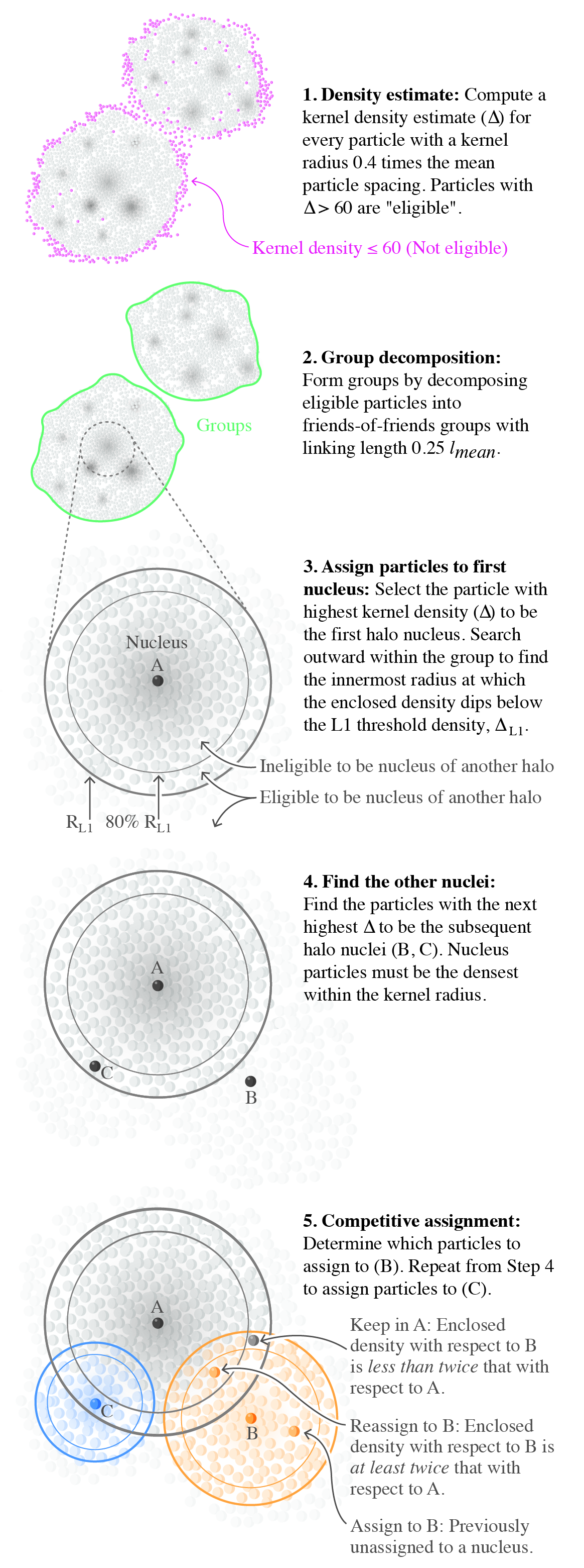
Figure 1: Visualization of the CompaSO algorithm detailed in Section 2.2.

2.3 Optimization and implementation

In the following, we describe particular features of the implementation of our algorithm, which have helped us to significantly speed up the halo finding process.

2.3.1 Density scaling with redshift

For Einstein deSitter cosmology, the density threshold for L1 and L2 haloes are $\Delta_{\rm L1}=200$ and $\Delta_{\rm L2}=800$, respectively. As the cosmology departs from Einstein deSitter, we scale upward the density threshold for L1, $\Delta_{\rm L1}$ in order to keep in agreement with spherical collapse estimates for low-density universes. The FoF linking length, $l_{\rm FoF}$, is scaled as the inverse cube root of that change, while The kernel density smoothing scale, $b_{\rm kernel}$, remains unchanged. We make use of the redshift scaling of the fitting function provided by Bryan & Norman (1998), which defines the density with respect to the critical density as:

$$\Delta_{\rm base}(z)=18\pi^{2}+82x-39x^{2},$$ (2)

where $x=\Omega_{m}(z)-1$ and $\Omega_{m}(z)$ is the matter energy density at redshift $z$ and $\Delta_{\rm L1}(z)=(200/18\pi^{2})\Delta_{\rm base}(z)$ is the corresponding density threshold $\Delta_{\rm L1}(z)$ relative to the critical density at a given redshift $z$ . Equivalently, in the case of L2 haloes, it is determined by the relation $\Delta_{\rm L2}=(800/18\pi^{2})\Delta_{\rm base}$. Throughout the paper, we will refer to overdensities defined using the Bryan & Norman (1998) scaling relation as “virial.” The default mass definition of the ROCKSTAR algorithm also adopts the Bryan & Norman (1998) fitting formula.

2.3.2 Density-radius relation

For our estimates of the enclosed density of a particle with respect to an existing nuclei, we do not compute its exact value, but rather use a fitted model of the relation between the density and radius. This speeds up the code significantly for two main reasons: (a) it avoids having to do a complete sort on the distances (which we never do for finding the L1 radius), and consequently, (b) it avoids having to permute those enclosed densities back into the original particle order, which would incur disordered memory access.

Our fitted model is as simple as assuming a flat rotation curve based on the L1 radius, so the enclosed density is

$$\Delta_{\rm encl.}(r)=\Delta_{\rm L1}\frac{R_{\rm L1}^{2}}{r^{2}}.$$ (3)

We emphasize that this relation is only being used to deblend zones between haloes. The actual halo boundary for any unblended region is still taken to be the L1 enclosed density radius (based on all particles, not just members).

2.3.3 Distances computation

The algorithm is sped up by storing the position and original particle index in a compact quad of floats, aligned to 16 bytes to aid in the vectorization (see Maksimova et al., 2021; Garrison et al., 2021, for details on the implementation). We store the index as an integer; when interpreted bitwise as a float, it becomes a tiny number. We then compute the square distances in the 4-dimensional space, as this is faster with the vector instructions.

Note that throughout the CompaSO algorithm, we work with square distances (rather than linear ones), so as to avoid taking many square roots. Furthermore, we track the inverse enclosed density because we can compute it directly without having to take its reciprocal. Searching for the enclosed density threshold is logically equivalent to sorting the distance list and searching outwards until one finds the element for which the index in the sorted array exceeds the cubed distance (assuming the particle mass is unity, the index number is equivalent to the enclosed mass).

2.3.4 Threshold radius search using cells

The most straightforward implementation of the algorithm in Section 2.2 involves sorting the whole list and looking for the threshold radius $R_{\rm L1/L2}$, but usually we do not need to go far from the nucleus to find this radius. Therefore, sorting the entire list is unnecessary effort, as it is a $\mathcal{O}(N\log{}N)$ process, while doing a single partition is only $\mathcal{O}(N)$. Instead, one can do a partitioning on a square radius and determine that the mass interior to that radius does not reach the density threshold, repeating that process until the threshold radius is found.

This is precisely what we use to optimise the inside-out radius search. Internally, Abacus has already ordered the particles in terms of their cell membership, i.e. their bounding boxes. We can thus use the the cell boundaries positions to compute the minimum and maximum bounds for each cell, and we also know the mass in each group. Working outward in steps of $\sqrt{3}/3L$ (radial bins), where $L$ is the cell size, yields at most 3 crossings (or two bisection passes) per cell. Note that this needs to be done only for the cells that satisfy the condition for threshold radius search. We determine this in the following way: if we place the mass contained within the interior edge of the radial bin under consideration at the exterior edge of that radial bin and find that it satisfies the density threshold, then we know that the searched-for radius cannot be inside that radial bin. If the mass does not satisfy the threshold, then we have to search within it. Note that in the case where the search fails, we simply need to keep looking outwards. The innermost radial bin will always satisfy the condition for threshold searching.

2.3.5 Comparative sweep and collection of particles into group order

In our algorithm, we need to have a way of denoting whether a given particle is eligible to become a halo center (nucleus) and also what its current halo affiliation is (i.e. which existing halo it has been assigned to most recently). To do so, we create a single array that combines the group identification number and active flag into one integer. The absolute value of the integer indicates the index of the halo nucleus it is assigned to and negative integer means that the particle is ineligible to become a halo nucleus. This saves computation time since we reduce the number of variables which need to be swapped and sorted.

We finally sweep through the particles to segment them (by partitioning them based on their halo affiliation index) into groups. A simple optimization we have applied is to first partition for the first halo, as it is most likely to be the largest. Then before going to the second, we partition to sweep all of the unassigned particles, so that we do not have to pass through them again. This is because in most cases the largest halo particles and the unassigned particles are the two biggest sets and getting those out of the way before we segment the other haloes helps save computation time.

Code notation	Paper notation	Value	Description
BoxSize	$L_{\rm box}$	1 Gpc$/h$	Size of the simulation box
NP	$N_{\rm part}$	$3456^{3}$	Number of particles in the box
ParticleMassHMsun	$M_{\rm part}$	$2.109\times 10^{9}\ M_{\odot}/h$	Mass of each dark matter particle
Omega_M	$\Omega_{m}$	0.315	Energy density of the total matter in the Universe at $z=0$
FoFLinkingLength	$l_{\rm FoF}$	0.25	Linking length for the modified FoF
MinL1HaloNP	$N_{\rm L1,min}$	35	Minimum number of particles in the L1 halo for including in halo catalogue
L0DensityThreshold	$\Delta_{{\rm L0,min}}$	77.5	Minimum kernel density for a particle to be part of an L0 group (scaled to 60)
SODensityL1	$\Delta_{\rm L1}$	258.2	L1 halo density threshold at $z=0.5$ (scaled to 200)
SODensityL2	$\Delta_{\rm L2}$	1033.0	L2 halo density threshold at $z=0.5$ (scaled to 800)
DensityKernelRad	$b_{\rm kernel}$	0.4 $l_{\rm mean}$	20cmThe scale over which a new nucleus must have highest
kernel density $\Delta$ in units of the mean interparticle distance, $l_{\rm mean}$/
The smoothing scale of the weighting kernel $W(r;b_{\rm kernel})$
used for computing the density of each particle
SO_RocheCoeff	$c_{\rm Roche}$	2	20cmFactor for attributing particle to new nucleus
motivated by the tidal radius condition
SO_NPForMinDensity	$N_{\rm new,min}$	35	Kernel density criterion for ceasing to look for new nuclei
SO_alpha_eligible	$R_{\rm L1,elig}$	80% of $R_{\rm L1}$	20cmRadius for determining the eligibility boundary of new
nuclei in units of the L1 threshold radius $R_{\rm L1}$
ParticleSubsampleB	Subsample B	7%	Percentage of particles output in Subsample B
N	$N$	—	Number of particles in the L1 halo
r_XX_L2com	$r_{\rm XX}$	—	20cmRadius within which XX% of the L1 halo particles
are contained wrt the particle center of the first L2 halo
r_50_L2com	$r_{\rm halfmass}$	—	20cmRadius within which 50% of the L1 halo particles
are contained wrt the particle center of the first L2 halo
r_98_L2com	$r_{\rm halo}$, $r_{98}$	—	20cmRadius within which 98% of the L1 halo particles
are contained wrt the particle center of the first L2 halo
SO_central_particle	L1 particle	—	Particle center of the L1 halo
SO_L2max_central_particle	L2max particle	—	Particle center of the first L2 halo
x_com	L1 com	—	Center-of-mass of the L1 halo
x_L2com	L2max com	—	Center-of-mass of the first L2 halo
vcirc_max_L2com	$V_{\rm max}$	—	The maximum circular velocity any particle in the L1 halo attains
rvcirc_max_L2com	$r_{\rm v,max}$	—	The radius at which the maximum circular velocity is reached

Table 1: Names of the variables as they appear in the Abacus code and in this paper, accompanied by short descriptions. The corresponding values are also provided for the box used in this analysis, AbacusSummit_highbase_c000_ph100. The first set of variables can be found in the Header files of the individual simulations, whereas the second set can be found in the field names of the halo catalogues.

3 Catalogue cleaning

In this section, we explore the robustness of the CompaSO halo catalogues. As is the case for all configuration-space finders, CompaSO has to deblend haloes in close proximity to each other without using velocity information of the particles. In some cases, this results in the algorithm defining unphysical objects as haloes (as illustrated in Fig. 3), which should instead be merged into nearby haloes or altogether discarded. Some halo finders try to address this problem by taking additional steps: e.g., performing particle unbinding or using merger tree information. In the case of CompaSO, we opt to perform cleaning of the halo catalogues in post-processing, as detailed in Bose et al. (2021) and summarised below. In this section, we test how robust the cleaned catalogues are, comparing and complementing them with additional consistency checks. In particular, we test the persistence of haloes through time and the presence of particles with excessively high velocities, as measures of their “trustworthiness”. We show that while the cleaning does not fix all issues, it certainly gets rid of the majority of problematic haloes. Additional cleaning of the catalogues can be performed using already existing halo statistics.

3.1 Cleaning method

The choice of whether an object is identified as a halo by any halo-finding algorithm can be somewhat arbitrary. In the case of SO-based methods, the halo boundary is set starkly by the SO threshold density, while for FoF-based finders, it is strongly dependent on the linking length parameter. This choice becomes even more challenging in dense regions of the simulation as well as during halo merging and splashback events. A frequent interaction between a satellite halo orbiting around a larger companion is the expulsion of the satellite after several time steps. This typically results in a significant reduction of the mass of the expelled object, as it is stripped of its outermost layer. The inner dense core of the halo, which is also expected to be the location that the baryons would occupy in a realistic full-physics setting, would be less prone to tidal stripping. However, an empirical population model such as the halo occupation distribution (HOD) model applied after the satellite gets expelled would underweight it and assign a galaxy to it based on its “present-day” mass. This could clearly result in non-physical outcomes, where e.g. prior to a two-halo interaction, the HOD prescription predicts two galaxies, but a few snapshots later, when the smaller halo gets expelled by the larger one and stripped of its outer shell, the HOD prescription attributes a single galaxy to the two-halo system.

Since one of the main goals of the AbacusSummit project is to provide the DESI collaboration with a suite of simulations for creating mock catalogues via empirical models, our focus is on adapting the final products to suit those needs by ameliorating some of the aforementioned issues. To this end, we provide our users with a “cleaned” version of the CompaSO catalogues. The procedure for cleaning the catalogues is detailed in Bose et al. (2021). and relies on utilizing merger-tree information about each halo. There are two types of merger-tree outputs we have combined in an attempt to weed out unhealthy haloes: a flag that marks “potential splits” and the ratio between the peak halo mass and the present-day halo mass. The first flag checks the consistency of the halo by tracing its main progenitors in previous steps and tracking what percentage of the particles are shared between the main progenitor and the present-day halo. If the number is unphysical, i.e. the present-day halo received most of its particles from a much larger halo in the previous time step and therefore cannot be its main descendant, we mark this halo as a “potential split” (IsPotentialSplit flag in the merger tree catalogues). The second way in which we diagnose these halo-finding pathologies is by declaring unphysical all haloes for which the peak mass exceeds the present day mass by more than a factor of $\kappa=2$ (see Bose et al., 2021, for details). We merge haloes that have failed either of the above criteria into other nearby haloes from which they have presumably split off and record the updated halo masses (the haloes that are merged donate their entire mass to the object they are merged into). We show halo mass and correlation statistics of the cleaned CompaSO catalogues in Section 4.1 and Section 4.3. In very rare cases ($\sim 0.1\%$), the MainProgenitor of a halo marked for cleaning may not be identified correctly, so we search for its true main progenitor in the complete Progenitors list and merge it onto that object.

3.2 Persistence of haloes through time

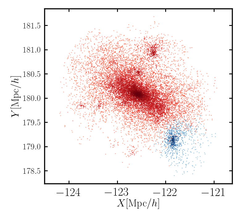
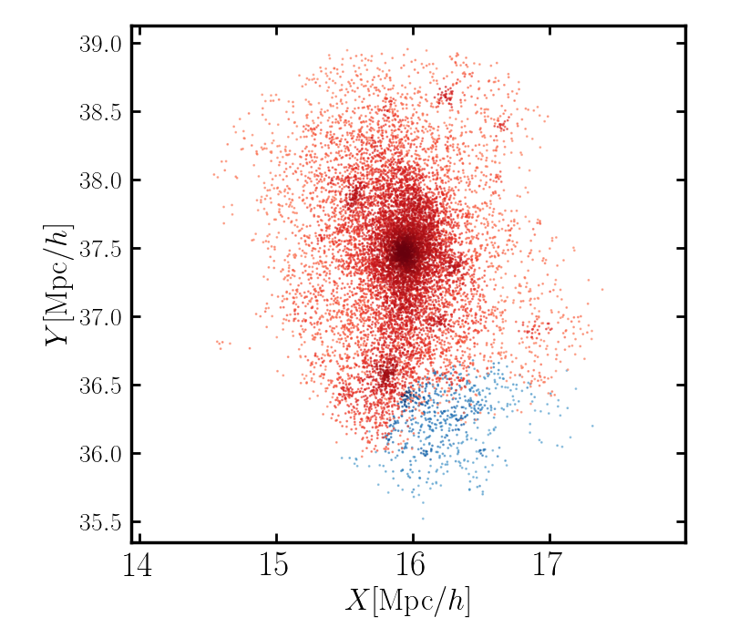
Figure 2: Scatter plots of haloes identified as “potential splits” (blue dots) and their central (largest) companions in the vicinity (red dots). The left panel shows an example in which the “potentially split” halo does have a dense core, distinct from that of its companion. In this case, the smaller halo has been orbiting in close proximity to the larger one for several snapshots (during which the algorithm has identified the two as a singular object) after which it has been expelled. The right panel shows a case of a non-physical “potential split” for which the small halo is lacking a dense center of particles. A “potential split” is defined as an object which in the previous time step, was considered part of a larger halo, but in the last time step, has been split by the CompaSO algorithm. Objects lacking a well-defined core can be isolated by using diagnostics combining the merger tree flag IsPotentialSplit (see statistics for how often these occur in Table 2) and the ratio of the radius containing all the particles to $r_{{\rm v,max}}$ (see Fig. 3). The scatter plots are using 3% of the halo particles.

A powerful test of the “reality” of the small haloes found on the outskirts of big ones is their persistence between redshift slices. In other words, we can potentially track satellite haloes at $z=0.5$ and check if they were present at earlier times. For these smaller haloes, the effects which contribute to their disruption and inconsistency throughout the merger history are both physical as well as algorithmic. Smaller haloes are less likely to survive flybys past larger haloes because their cores are less dense and thus more easily destructible. Another frequent interaction between a satellite and a central halo is the expulsion of the satellite by the larger halo, which typically significantly reduces the mass of the expelled object, stripping it of its outermost layer. In addition, sometimes dark-matter substructure on the outskirts of large haloes may have been identified as an autonomous halo by the CompaSO algorithm at a given snapshot, but this object might not have a distinct merger history. In this section, we examine how often we find such occurrences by using statistics output by the accompanying merger tree associations (Bose et al., 2021).

In Fig. 2, we demonstrate two cases of haloes that have been marked as “potential splits” (see Section 3.1 for a definition). On the left panel, we show a case of a non-physical algorithmic split while on the right panel, the smaller halo has a healthy core and has only spent a small portion of its history as part of its larger companion (but otherwise has a distinct history). In Table 2, we show the percentage of “potential splits” for different mass ranges in the third column. We see that their numbers are very small in particular on the high-mass end ($\log(M)>13.7$), where they are less than 0.004%. The overall percentage is around 12% and it is highly dominated by the smallest haloes ($\log(M)\sim 10^{11}$). The reason for this relatively larger percentage is that for less massive objects flying through dense regions, the boundary is harder to draw, as they have less dense cores and are more difficult to distinguish from the background. This is less and less frequent at higher halo masses.

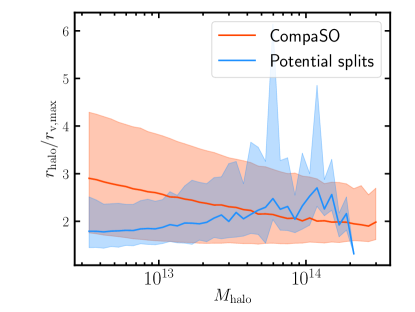
Figure 3: Ratio of the radius containing all halo particles to the radius where the maximum circular velocity is attained, $r_{{\rm v,max}}$. We see that the haloes flagged as “potential splits” have a distinct $r_{\rm halo}/r_{{\rm v,max}}$ distribution (blue shaded curve) compared with the typical CompaSO population (red shaded curve). This indicates that looking at ratios of the inner and outer halo radii can help us diagnose problematic cases, since for these haloes their centers are typically not correctly identified.

$\log(M)$ range	Number of haloes	Main Prog. matching at $z=0.875$	Main Prog. matching at $z=1.625$	“Potential splits”
$11.5\pm 0.1$	5096084	94.8%	73.1%	10.5%
$12.5\pm 0.1$	610240	96.7%	91.4%	7.86%
$13.5\pm 0.1$	46585	96.9%	89.9%	5.11%
$14.5\pm 0.3$	2823	96.3%	85.3%	0.42%
all haloes	24721876	89.7%	64.2%	12.8%

Table 2: Merger trees statistics for the haloes at $z=0.5$ using the AbacusSummit merger trees associations (Bose et al., 2021). The first two columns of the table show the mass range selected as well as the number of CompaSO haloes in it at $z=0.5$. The next two columns show what percentage of these haloes’ main progenitors inferred through the “fine” tree associations agree with those inferred using the “coarse” tree ones at $z=0.875$ and $z=1.625$, respectively. The last column displays what percentage of the haloes are identified as “potential splits” by the merger tree algorithm in each of the mass sets.

Another reliable diagnostic is to examine the persistence of haloes across longer periods of time. The simulation products include merger histories based upon stringing together consecutive snapshots and thus obtaining a full merger tree, which we also dub as “fine.” Additionally, one can also utilise the “coarse” trees built over non-adjacent time steps, spanning longer time epochs. To illustrate, the next two steps of the “coarse” merger trees for haloes at redshift of $z=0.5$ are at $z=0.875$ and $z=1.625$. One of the “realness” criteria for the haloes at $z=0.5$ we propose is to compare their progenitors at earlier times and note how often their “coarse” and “fine” histories point to the same progenitor. We do this at time steps $z=0.875$ and $z=1.625$ and display the results in the first and second columns of Table 2. At $z=0.875$, the progenitors of the haloes at $z=0.5$ match at $\gtrsim 95\%$ at the mass scales typically of interest for creating mock catalogues (i.e. $\log(M)\sim 11.5$ and higher) and close to 90% for the entire halo population. haloes for which we find a match can be certified as “healthy,” though we should not be discarding those for which no match, as there could be multiple reasons for this (e.g., a halo has orbited inside a larger companion for a significant portion of its life and as a result has lost a substantial amount of mass, which has caused the step-by-step merger tree to fail at tracing its history). At $z=1.625$, the percentages are noticeably lower. For the high-mass objects, they are close to 90%. However, we note that on the low-mass end, oftentimes the haloes have not yet been formed at these earlier redshifts, so the merger tree “fine”-to-“coarse” comparison might not be an accurate test of persistence.

There are potentially other ways to spot and diagnose unphysical haloes. As mentioned above, some objects are identified by the CompaSO algorithm as distinct haloes while in reality they may lack a dense core and might simply be carved out of a nearby companion due to the SO boundary. For these objects, the ratio between radial quantities such as $r_{\rm halo}$ and $r_{\rm v,max}$ will most likely be atypical compared with the rest of the population at that mass scale. In Fig. 3, we demonstrate what the distribution looks like for haloes flagged as “potential splits” by the merger tree algorithm and the rest of the population. We can notice that the ratios are particularly different for the lower halo masses, which is also where we expect to find most of the unphysical algorithmic choices. On the higher mass end, the “potential splits” are more consistent with the general population. As discussed, some of the objects labelled “potential splits” may in fact be “real” haloes expelled after orbiting a companion halo (particularly for haloes with denser cores and more particles), so a more robust way of “pruning” the merger tree would involve flagging objects with odd ratios of their radial quantities which have also been identified as “splits.”

3.3 Presence of high-velocity particles

A problematic mode for many halo finders is the deblending of close pairs of haloes with a large mass ratio, where particles get assigned to one halo, even though they may not be bound to that halo. Neglecting the presence of these particles may bias the inferred properties of the haloes such as their spins and velocity dispersions. A way to identify such failed cases is by locating particles with high infall velocities. Some configuration-space-based finders address this issue by performing energy-based unbinding, but in the case of CompaSO, we opt not to perform particle unbinding because of both the speed requirement of Abacus and the problems associated with it, some of which we mention below. Instead, we adopt alternative strategies for cleaning the halo catalogues (see Section 3.1). In this section, we analyse the cleaned catalogues in terms of their effectiveness in removing haloes with a large presence of high-velocity (“unbound”) particles. We verify that indeed after the cleaning, very few problematic haloes remain in the catalogues. In addition, we find alternative statistics that help us weed out unphysical haloes that were missed in the cleaning.

Energy-based unbinding is typically done to discard particles that are tentatively assigned to a particular (sub)structure, but do not appear gravitationally bound to it. For subhaloes, removing unbound particles is of particular importance, since their particle lists are often contaminated with particles from the host halo due to the relatively lower density of the subhalo. This can influence significantly the inferred subhalo properties such as its mass and dispersion velocity. Similarly, interacting haloes often acquire stray particles whose velocities are too high to keep them bound to their host. Standard unbinding treats every halo individually and removes all particles whose kinetic energies exceed their potential energy.

However, there are several well-known issues associated with energy-based unbinding. The presence of particles with high velocities inside the boundaries of the halo is often a consequence of close fly-bys with other haloes. Therefore, the high-velocity particles should instead be assigned to a neighbour (which is also the spirit of the competitive assignment algorithm for CompaSO and the cleaning procedure). In standard unbinding, these particles are usually returned to the next level up the halo hierarchy, but when applying unbinding to halo hosts, the unbound are altogether deprived of halo membership rather than merged onto a close neighbour. The unbinding procedure assumes that the halo is isolated, and any effects that arise from outside, e.g. particles on the edges, interactions, tidal effects, are neglected. In particular, even particles in isolated haloes whose orbits take them outside of the arbitrarily defined “halo radius” have their ability to return underestimated because the mass contribution from the particles outside is neglected (we address this below). In addition, in the case of interacting haloes (e.g, two haloes orbiting around each other, or falling into each other), calculating the potential of each particle with respect to a single halo would not be reflective of the gravitational forces experienced by the particle. Enlarging the scope and considering the global potential of the simulation, on the other hand, is also not the correct quantity to use, as it is large-scale dominated and does not answer the question of whether the particle is bound to a particular halo. The simplification of ignoring interactions is also motivated by the enormous computational expense that would arise from taking the entirety of structures in the computational domain into account for each structure anew. A more precise approach involves boosting the gravitational potential to make it a locally meaningful quantity, which can be used to define a binding criterion that incorporates the effect of tidal fields (Stücker et al., 2021).

We test the effect of applying energy-based unbinding to the CompaSO catalogues of a small test simulation with box size $L_{\rm box}=296\ {\rm Mpc}/h$ and particle mass $M_{\rm part}=2.1\times 10^{9}\ M_{\odot}/h$, containing 1.3 million haloes. We also apply the ‘cleaning’ procedure from Section 3.1 and Bose et al. (2021), which identifies 1.6%, or 21000, of the haloes in the simulation as ‘unphysical’. We perform the process of unbinding iteratively for each halo in its centre of momentum frame of its core, i.e. subtracting $\mathbf{x}_{\rm L2com}$ and $\mathbf{v}_{\rm L2com}$ from the position and velocity of each particle, $\mathbf{x}$ and $\mathbf{v}$. All comoving positions are converted into proper coordinates, and the Hubble flow term is added to the particle velocities, $H(z)(x-x_{\rm L2com})$. We compute the spline potential adopted by Abacus (Garrison et al., 2021) at each iteration, discarding the particles with kinetic energies higher than their potential energies. This process continues until no more particles are found to be unbound.

In addition, we propose a simple, yet well-motivated modification to the standard unbinding algorithm, which ameliorates the issue of the arbitrary drawing of halo boundaries. Let us imagine an isolated halo whose density profile follows an NFW distribution. Typically, we define the halo boundaries, $r_{\rm vir}$, by requesting that the enclosed density is $X\times\rho_{\rm crit}$. In the case of CompaSO, the ‘virial mass’ is defined using the Bryan & Norman (1998) scaling relation (see Section 2.3). Nevertheless, the particles outside $r_{\rm vir}$ still contribute to deepening the potential well of the halo despite not strictly belonging to it. Not accounting for this outside contribution would lead us to falsely discard bound particles that, as a result of the deepening of the potential, are in thermal equilibrium despite their higher velocities. This extra contribution to the potential, $\phi_{\rm extra}$, assuming a spherical halo, is computed below for an NFW profile.

$$\phi_{\rm extra}=\int_{r_{\rm vir}}^{\infty}\frac{4\pi G\rho_{\rm NFW}(r)r^{2}}{r}dr=-\frac{GM_{\rm vir}}{r_{\rm vir}}\frac{c/(c+1)}{A_{\rm NFW}},$$ (4)

where $A_{\rm NFW}\equiv\ln{(1+c)}-c/(1+c)$, $x\equiv r/r_{\rm vir}$, and $c$ is the halo concentration. Simplifying this, we get:

$$\phi_{\rm extra}=-\frac{GM_{\rm vir}}{r_{\rm vir}}[\ln({1+c})(c^{-1}+1)-1]^{-1}\equiv-\frac{GM_{\rm vir}}{r_{\rm vir}}f(c)$$ (5)

and show the function $f(c)$ in Fig. 4. We note that in the case of elliptical haloes, the assumption of spherical shapes tends to underestimate the contribution of the outside potential and its ability to stabilise the particles on the edges of the halo. Nevertheless, to approximately account for this effect, we add the term $\phi_{\rm extra}$ to the potential energy of each halo when removing unbound particles. As demonstrated in Fig. 8, the truncated NFW profile is a good approximation to the CompaSO halo profiles. We thus obtain the halo concentration $c$ by fitting an NFW profile to every halo. For haloes for which a fit cannot be obtained (mostly small haloes, making up less than 3%), we approximate the concentration as $r_{100}/r_{10}$.

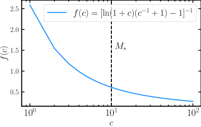
Figure 4: Factor $f(c)$ determining the magnitude of the extra potential term as a function of concentration, as derived in Eq. 5. Less concentrated haloes receive a larger contribution to their potentials from particles lying outside $r_{\rm vir}$ compared with more highly concentrated haloes. The black vertical dashed line shows roughly the concentration of Mily-Way-like haloes. We note that halo concentration and halo mass are weakly anti-correlated.

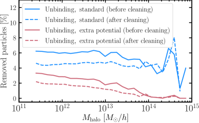
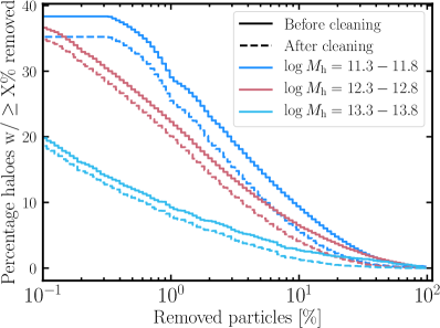
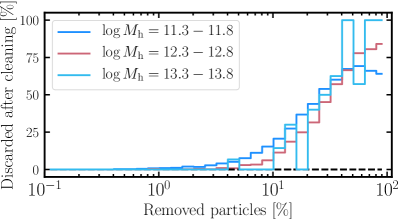
Figure 5: Top panel: Average percentage of removed particles through unbinding as a function of halo mass. In blue, we show the result when performing the standard cleaning procedure (see Section 3.1 and Bose et al. (2021)), whereas in red, we show the outcome when adding an extra term to the potential energy, $\phi_{\rm extra}$ (see Eq. 5). The percentage of removed particles is significantly reduced (top panel) when including $\phi_{\rm extra}$ – by a factor of $\sim$ 2 for smaller haloes and $\sim$ 10 for higher-mass haloes. Similarly, when we remove the discarded haloes (dashed lines), the average percentage of removed haloes drops further. The objects that are cleaned away make up 1.6% of all haloes in the simulation. Middle panel: Cumulative percentage of haloes as a function of removed particles before and after cleaning for three different mass bins: $\log(M_{\rm halo})=11.3-11.8$, $\log(M_{\rm halo})=12.3-12.8$, and $\log(M_{\rm halo})=13.3-13.8$. We see that 38%, 36% and 30% of the before-cleaning haloes for these mass bins have more than 0.1% of their particles removed, while 10%, 7% and 3$, respectively, have more than 10% removed. The cleaning reduces these numbers by several per cent. Bottom panel: Percentage of retained haloes after cleaning as a function of removed particles for three different mass bins. It is encouraging to see that the cleaning weeds out an increasingly larger number of haloes (close to 100% for the highest mass bin shown), as we consider haloes with an increasingly large number of “unbound” particles.

In the top panel of Fig. 5, we show the averaged percentage of removed particles as a function of halo mass when we apply the standard unbinding procedure and the $\phi_{\rm extra}$-augmented procedure (see Eq. 5). We see that the standard procedure removes 6.5% of the particles in smaller haloes and 4% of the particles in higher-mass haloes. These number are significantly reduced when including the $\phi_{\rm extra}$ term, to 3.5% and 0%. Additionally, we discard the haloes considered ‘unphysical’ by the cleaning procedure of Section 3.1 and Bose et al. (2021), noting that the average percentage of removed particles is brought down by nearly 1-2% for $M_{\rm halo}<10^{14}\ M_{\odot}/h$. This implies that there is an overlap between haloes with a large percentage of removed particles and the haloes that were cleaned away. To test this, in the middle panel, we show the cumulative percentage of haloes with more than X% “unbound particles” for three mass bins and find that the majority of haloes have less than 0.1% removed particles, with higher mass bins performing better. Overall, as also illustrated in the bottom of Fig. 5, the cleaning makes a big difference, removing very effectively haloes that have more than 10% “unbound particles”. For the higher masses, the cleaning is even more efficient and removes up to 100% of the haloes with a large unbound particle population. If the cleaning procedure from Section 3.1 is regarded as reliable, then this finding suggests that the unbinding procedure augmented with an extra potential term yields a more robust halo catalogue compared with the standard unbinding procedure.

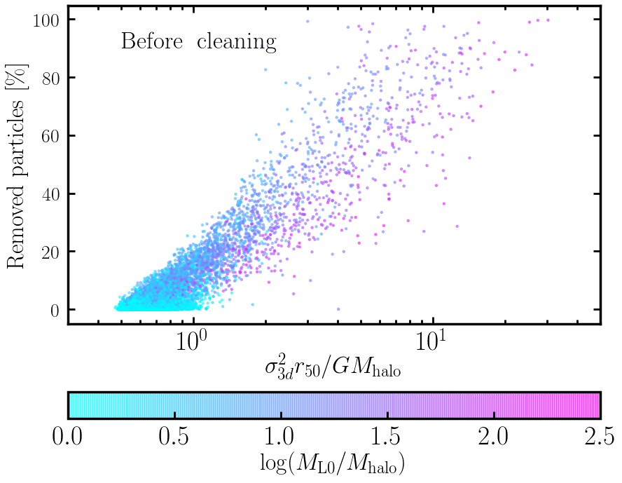
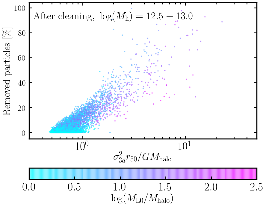
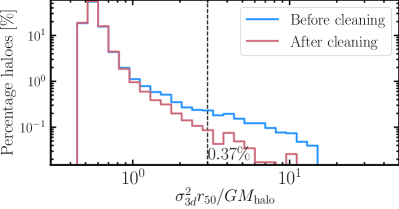
Figure 6: Coloured scatter plot of the percentage of removed particles due to unbinding as a function of the virialisation parameter, defined as $\sigma^{2}_{3d}r_{50}/GM_{\rm halo}$. The colour denotes the ratio of the mass of the “L0” parent group and the halo mass, $\log(M_{\rm L0}/M_{\rm halo})$, with purple corresponding to a high ratio and blue corresponding to a low ratio. The plot shows all haloes in the range $\log M_{\rm halo}=12.5-13.0$, measured in units of $M_{\odot}/h$, before applying the cleaning procedure (top panel) and after (middle panel). We see a strong positive correlation between the virialisation ratio and the percentage of removed particles, suggesting that a viable mechanism for cleaning the halo catalogues in addition to the default CompaSO cleaning may involve discarding haloes with a high virialisation parameter ($\gtrsim$ 2-3). Furthermore, haloes with a high ratio $\log(M_{\rm L0}/M_{\rm halo})$ tend to lose a higher percentage of their particles to unbinding, indicating that the most problematic mode of CompaSO is the assignment of particles to haloes in a cluster. In the bottom panel, we show the percentage of haloes as a function of virial ratio before and after cleaning. Haloes to the right of the dashed black line account for 0.37% of all haloes after cleaning in the mass bin. This demonstrates that the cleaning takes care of the majority of bad actors and leftover objects can be discarded by combining output statistics such as the virialisation parameter and the cluster mass ratio.

In addition, we test the conjecture that unphysical objects (e.g., haloes with a bimodal profile or haloes lacking a nucleus) can be identified through other internal halo properties that are already being output. In Fig. 6, we consider two such quantities. The first one is the virial ratio $\sigma_{3d}^{2}r_{50}/GM_{\rm vir}$, where $\sigma_{3d}$ is the three-dimensional dispersion velocity. Fig. 6 indicates that there is a very strong correlation between haloes with a large percentage of unbound particles and a large virial ratio. One can therefore imagine augmenting the cleaning procedure with a requirement that the halo virial ratio does not exceed a certain threshold such as 2 or 3, which as seen in the figure for the bin $\log(M_{\rm halo})=12.5-13.0$, gets rid of the majority of offenders. In fact, after performing the cleaning, only 1.14% of the haloes with mass $\log(M_{\rm halo})=11.5-12.0$, 0.63% of the haloes with mass $\log(M_{\rm halo})=12.0-12.5$, 0.37% of the haloes with mass $\log(M_{\rm halo})=12.5-13.0$, 0.19% of the haloes with mass $\log(M_{\rm halo})=13.0-13.5$, 0.038% of the haloes with mass $\log(M_{\rm halo})=13.5-14.0$, and none above $\log(M_{\rm halo})=14.0$, are retained that have virial ratio above 3. All masses are reported in units of $M_{\odot}/h$.

We conjecture that this is due to issues that CompaSO has with deblending haloes in close proximity and in particular, with determining the boundaries of small haloes near larger ones. To test this, we have colour-coded the points in Fig. 6 by the logarithmic ratio of the “L0” parent group mass and the halo mass, $\log(M_{\rm L0}/M_{\rm halo})$, with small haloes living in large halo clusters having large $\log(M_{\rm L0}/M_{\rm halo})$ ratio. Fig. 6 shows that the vast majority of haloes with high percentage of removed particles (and thus high virial ratio), have high ratio $\log(M_{\rm L0}/M_{\rm halo})>1.5$. A sensible and easy solution to this issue is thus to discard these small haloes rather than try to remerge them, as their contributions to the masses of large nearby structures are negligible. Additionally, we perform visual inspection of hundreds of these objects and find that the majority of the leftover haloes have well-defined nuclei with extended envelopes that likely contain some number of particles that are gravitationally bound to nearby massive structures.

We conclude that the cleaning mechanism (from Section 3.1 and Bose et al. (2021)) takes care of the vast majority of unphysical objects and that remaining wrongdoers can be identified and discarded (or remerged into the main progenitor branch) through their higher virial and/or mass ratios during postprocessing.

4 Halo analysis

In this section, we analyse the properties of the haloes derived through the CompaSO algorithm using the AbacusSummit_highbase_c000_ph100 simulation. This simulation contains $N_{\rm part}=3456^{3}$ dark matter particles in a box of size $L_{\rm box}=1$ Gpc$/h$, which corresponds to a particle mass resolution of $M_{\rm part}=2.109\times 10^{9}\ M_{\odot}/h$. For the subsequent investigation of halo properties, we have chosen to focus on the redshift slice at $z=0.5$ and have also obtained an alternative halo catalogue in post-processing via the phase-space halo finder ROCKSTAR. We compare the two halo finders in terms of their halo mass functions, auto- and cross-correlation functions, and radius-mass relationships. We further study the density profiles of the CompaSO haloes and alternative definitions of their halo centers. In the mass range $M=10^{12}-10^{15}M_{\odot}/h$, the ROCKSTAR halo catalogue contains a total of haloes of 4,137,230, while CompaSO has 4,016,661. Throughout this section, the masses of objects are presented in units of $M_{\odot}/h$.

Short descriptions of the relevant quantities for the halo analysis are displayed in Table 1 along with the corresponding notation for the halo catalogue fields in the AbacusSummit output products.

4.1 Halo mass function

The halo mass function is central in cosmology, as it describes how many haloes of a given mass exist at a given redshift. Obtaining this information is important since dark matter haloes play an essential role in modeling galaxies and galaxy clusters and thus, in studying large-scale structure. The halo mass function allows us to understand the statistics of primordial matter inhomogeneities and is also used to compute the effects of nonlinear structure on observations through, for instance, the Sunyaev-Zeldovich effect and lensing. Another feature of the halo mass function is that it can be expressed as a universal function that relates the mass of haloes to the variance of the mass fluctuations (e.g. (Press & Schechter, 1974; Sheth & Tormen, 1999; Jenkins et al., 2001; White et al., 2001; Springel et al., 2005; Warren et al., 2006).

For our comparative analysis of halo algorithms, we compute the halo mass function at redshift $z=0.5$ using both the ROCKSTAR and CompaSO algorithms as

$$dN_{\rm halo}(M,z)\equiv N_{\rm halo}(M,z)\,d\log M,$$ (6)

where we have defined $dN_{\rm halo}$ as the number of haloes in the mass range $d\log M$.

The halo mass functions of CompaSO and ROCKSTAR are presented in Fig. 7 adopting virial mass in the top panel and maximum circular velocity in the bottom. The lower segment of each panel shows the fractional difference between the two curves with respect to the black ROCKSTAR curve. We note that we have imposed a mass cut of $M_{\rm min}=N_{\rm L1,min}\times M_{\rm part}=7.4\ 10^{10}\ M_{\odot}/h$, where $N_{\rm L1,min}=35$, on the ROCKSTAR haloes, since we output CompaSO haloes of only roughly that mass and above. We note that the difference in the choice of minimum mass accounts for the majority of the observed discrepancy of the halo mass function for the lowest-mass haloes ($\log(M_{\rm halo})<11$).

In the upper panel, the masses of the ROCKSTAR haloes are obtained by using the default ‘virial’ mass, $M_{\rm vir}$, which similarly to CompaSO, adopts the fitting function of Bryan & Norman (1998), while the raw CompaSO masses (in red) are defined as the total number of particles in a halo (N, see Table 1) multiplied by the particle mass. We also show in green the cleaned CompaSO catalogues (see Section 3.1). We can see that the CompaSO haloes exhibit a small excess ($\lesssim 10\%$) of low-mass haloes near $10^{11}\ M_{\odot}/h$ compared with ROCKSTAR. On the high-mass end ($\sim 10^{15}\ M_{\odot}/h$), the CompaSO catalogue displays a ($\sim 50\%$) deficiency of high-mass objects near $10^{15}\ M_{\odot}/h$ compared with ROCKSTAR. These differences are nearly two times smaller when using the cleaned CompaSO catalogues (see Bose et al., 2021, for a discussion). The remaining difference is most likely the result of the choice of density threshold ($\Delta_{\rm L1}$) and the competitive assignment we impose on the CompaSO haloes as described in Section 2.2. In the mass range where the vast majority of haloes reside ($\sim 10^{11}-10^{14}\ M_{\odot}/h$), the agreement is good (within 25%) for our particular application of creating mock catalogues via empirical models such as the HOD model, although there is a slight excess of smaller haloes in the cleaned CompaSO catalogue. This finding, together with the relative paucity of large haloes, may be an indication of a tendency of CompaSO to oversplit large DM structures into central haloes surrounded by multiple satellites in their outskirts. We examine this further in Section 4.3 and Section 3.2. We also show the resulting fractional difference when using the ‘strict SO’ ROCKSTAR mass definition (see ROCKSTAR documentation for more details) for the same virial density choice, demonstrating that our curves of the halo mass function are strongly dependent on the mass definition adopted.

In the lower panel, we show the number of haloes as a function of another popular choice for halo mass proxy, the maximum circular velocity $V_{\rm max}$. We can now see that the two halo functions are in a considerably better agreement – roughly within 5% of each other on all $V_{\rm max}$ scales. This finding suggests that the two halo algorithms find the same objects for the most part and that the observed differences in the upper panel can be largely attributed to halo boundary choices and mass definitions.

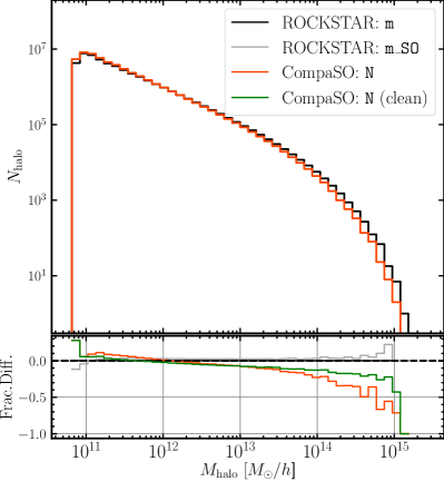
Figure 7: Halo mass functions of the ROCKSTAR and CompaSO groups. The upper panel shows the traditional halo mass function computed as the number of haloes as a function of halo mass for both finders. The black curve uses the ‘virial’ (default) mass definition of the ROCKSTAR finder, whereas the gray curve uses the ‘strict SO’ definition for the same choice of virial density. The red curve uses the CompaSO halo field N, corresponding to the total number of particles, multiplied by the particle mass, while the green curve uses cleaned haloes (see Bose et al., 2021, for details). The lower segment shows the fractional differences between each curve and ROCKSTAR. CompaSO haloes exhibit a small excess ($\lesssim 10\%$) of low-mass haloes compared with ROCKSTAR and a deficiency of high-mass objects. The cleaned CompaSO catalogues are in a better agreement with the ROCKSTAR halo mass function, exhibiting only half the discrepancy observed compared with the raw catalogues. The lower panel shows the number of haloes as a function of the maximum circular velocity. We see that the two halo functions are in a considerably better agreement – within $\sim$5% on all scales, suggesting that the two algorithms find the same objects for the most part.

4.2 Density profile

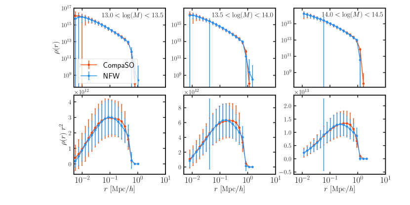
Figure 8: Average density profiles in three mass bins: 13 < $\log M$ < 13.5 (left panels), 13.5 < $\log M$ < 14 (middle panels), and 14 < $\log M$ < 14.5 (right panels), along with their respective averaged NFW fits. The upper panels shows the density profile, $\rho(r)$ in logarithmic space, while the lower panels show $\rho(r)r^{2}$, which is helpful for illustrating the mass differential ($dM/dr$) as well as the “knee” of the density profile, which is directly related to the concentration. The NFW-fitted concentration values for the three mass bins shown are $c_{\rm NFW}=[7.7,7.6,5.2]$, respectively.

According to Navarro et al. (1996), the density profiles of dark matter haloes in high-resolution cosmological simulations for a wide range of masses and for different initial power spectra of density fluctuations are well fitted by the formula

$$\rho_{\rm NFW}(r)=\frac{\rho_{\rm s}}{(r/r_{\rm s})\,(1+r/r_{\rm s})^{2}}$$ (7)

with $\rho_{\rm s}$ being the characteristic density and $r_{\rm s}$ the scale radius defined as

$$r_{\rm s}=\frac{r_{\rm vir}}{c}\ ,$$ (8)

where $r_{\rm vir}$ is the virial radius usually defined as the distance from the center of the halo to the outer boundary within which the mean density is $\sim 200$ times the present-day mean or critical density.

The concentration parameter introduced above describes the shape of the density profile, and in particular where the “knee” of the curve is located. From cosmological $N$-body simulations, extended Press-Schechter theory, and the spherical infall model, (Lokas, 2000; Bullock et al., 2001), we know that $c$ depends on the mass of the object and the form of the initial power spectrum of the density fluctuation. A well-known result is that higher mass objects have a lower concentration parameter and vice versa (e.g. Dutton & Macciò, 2014).

To study the particle distributions of the CompaSO haloes, we have computed the spherically-averaged density profiles of all haloes by binning the halo mass in equally spaced bins in log-space, between the virial radius and $\log(r/r_{\rm vir})=-2$. We are using 20 bins, which correspond to $\Delta\log(r)=-0.1$ and are sufficient to produce robust results. We compute the density profiles of haloes in the following 3 mass bins: $13<\log M<13.5$, $13.5<\log M<14$ and $14<\log M<14.5$ together with fits using the NFW profile. In this form, the NFW profile has two free parameters, $\rho_{s}$ and $c$, which are both adjusted through a least-squares minimization between the binned $\rho(r)$ and the NFW profile,

$$\sigma^{2}=\sum_{i=1}^{N_{\rm bins}}[\log(\rho(r_{i}))-\log(\rho_{\rm NFW}(r_{i},[\rho_{s},c]))]^{2},$$ (9)

where $r_{i}$ are the radial bins of the density profile, and $\rho_{s}$ and $c$ are the two parameters we are fitting for. Note that here we assign an equal weight to each bin.

The averaged density profiles and NFW fits of the haloes in the three mass bins are presented in Fig. 8. The top panels are displaying $\rho(r)$ as a function of distance with both axes in logarithmic space, while the bottom ones have $\rho(r)r^{2}$ as a function of distance. The latter are useful for seeing where the “knee” of the profiles is, while the former exemplify the typical power law expected from the NFW formalism and $N$-body simulations using alternative halo finders. We can see that the averaged NFW fits provide reasonably good fits to the halo profiles within the expected standard deviations across all haloes in each mass bin. The NFW-fitted concentration values for the three mass bins are $c_{\rm NFW}=[7.7,7.6,5.2]$, respectively, in accordance with the general expectation that concentration should decrease with mass. There are a few radial bins for which the error bars are substantially larger. Those are due to individual haloes whose density profiles follow an atypical form and thus, no good NFW fit has been found for them.

4.3 Two-point halo correlation functions

The two-point statistic is one of the most important probes of clustering in configuration space, and the main ingredient for the computation of the higher point statistics. The two-point correlation function, $\xi(r)$, is defined as the excess probability compared with a Poisson process of finding two objects at a certain spatial separation, $r$, (e.g. Bernardeau et al., 2002)

$$dP_{12}(r)=\bar{n}^{2}(1+\xi(r))\,dV1\ dV2$$ (10)

where $\bar{n}$ is the mean density. These objects in our case are the centers of the dark matter haloes. Clustered objects are indicated by $\xi(r)>0$, whereas objects are anticorrelated when $\xi(r)<0$. Eq. 10 can also be viewed as the conditional probability of having an object at $dV_{1}$ with a probability of $\bar{n}dV_{1}$ and of finding another object at distance $r$ in $dV_{2}$.

The auto-correlation functions in this work are estimated from $N$-body simulations using the natural estimator (Peebles, 1980)

$$\hat{\xi}(r)=\frac{\langle DD(r)\rangle}{\langle RR(r)\rangle}-1$$ (11)

where $\langle DD(r)\rangle$ and $\langle RR(r)\rangle$ are the normalised number of all possible pairs within the data and the random set, respectively.

Here we examine the two-point correlation functions of the haloes defined by the ROCKSTAR and CompaSO halo finders. We use two versions of the CompaSO catalogue: a raw version, which is directly taken from the simulation outputs, and a cleaned version, created for purposes of constructing mock catalogues and measuring correlation functions (for details about the cleaning procedure, see Bose et al., 2021). We do that by splitting the haloes into 5 bins: $\log M=11.5\pm 0.1$, $\log M=12.0\pm 0.1$, $\log M=12.5\pm 0.1$, $\log M=13.5\pm 0.1$, $\log M=14.5\pm 0.3$, respectively, with the mass measured in $M_{\odot}/h$. We also ensure that the number of ROCKSTAR objects is equal to the number of CompaSO objects in each set. We do this by rank-ordering the haloes in ROCKSTAR by mass and selecting all objects in the range $\log(M_{i})\pm[\Delta\log(M)]_{i}$, where $i$ is the current mass bin. We then similarly rank-order the CompaSO objects by mass and select the indices corresponding to the ROCKSTAR choice, adopting an abundance matching procedure. In this way, we can better normalise the correlation function on large scales and observe physical differences resulting from the halo definitions.

Figure 9: Two-point correlation functions of the ROCKSTAR (in black), CompaSO (in red), and cleaned CompaSO haloes (in green). The haloes are split into the following 5 bins: $1^{\rm st}\ {\rm bin}$: $\log M=11.5\pm 0.1$, $2^{\rm nd}\ {\rm bin}$: $\log M=12.0\pm 0.1$, $3^{\rm rd}\ {\rm bin}$: $\log M=12.5\pm 0.1$, $4^{\rm th}\ {\rm bin}$: $\log M=13.5\pm 0.1$, and $5^{\rm th}\ {\rm bin}$: $\log M=14.5\pm 0.3$, measured in $M_{\odot}/h$, and cross-correlations between each pair are shown. We see that there is an excess of CompaSO haloes around $\sim 1\ {\rm Mpc}/h$ relative to ROCKSTAR and the cleaned CompaSO catalogue, which implies that CompaSO is more likely to identify structures located in the outskirts of other haloes as separate haloes. We see a similar trend for the other two halo samples (ROCKSTAR and cleaned CompaSO) of finding a surplus of haloes around larger objects, but it is less pronounced than the raw sample.

In Fig. 9, we study the cross-correlations between each pair for the 5 mass bins defined above. This test serves to show us whether there is a significant number of haloes lurking on the outskirts of other, typically larger haloes. The correlation functions are given in Fig. 9 and suggest that the CompaSO halo finder is more likely to identify small dark matter structures and define them as distinct haloes on the boundaries of other haloes compared with the ROCKSTAR and cleaned CompaSO catalogues. We see this effect across all mass ranges, but most prominently for the highest mass sets, where CompaSO identifies the largest amount of substructure relative to ROCKSTAR (bottom row of the figure). The cleaned catalogue appears to be more similar to the ROCKSTAR one in terms of its halo clustering. It seems to contain more examples of large haloes orbiting other large haloes than ROCKSTAR, which suggests that large objects are oversplit (bottom right corner) while on the other hand, ROCKSTAR tends to identify more small haloes near large haloes (bottom left corner). Another feature of this plot is that the peaks of the correlation functions seem to be shifting towards larger scales as we go to higher-mass haloes (top to bottom), since these smaller haloes have correspondingly smaller radii. On the other hand, the locations of the peaks do not seem to change significantly for a given row. That is because the scale of the peaks is set by the average radius of the heavier haloes in a given cross-correlation panel.

4.4 Definitions of halo center

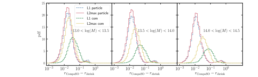
Figure 10: Difference between the various halo centers output by CompaSO and the “shrinking-sphere” halo center defined according to the method of Power et al. (2003). The haloes are split into three different mass bins: 13 < $\log M$ < 13.5 (left panel), 13.5 < $\log M$ < 14 (middle panel), and 14 < $\log M$ < 14.5 (right panel), measured in $M_{\odot}/h$. We see that the center of the first L2 halo, L2max, (denoted as L2max particle in the figure) is closest to the shrinking-radius definition (which we take as a proxy for the “true” density peak), while the center of mass of the L1 group (L1 com) exhibits the largest amount of scatter and is centered further away than the rest. Both particle center definitions, however, have a small locus of points located around $\Delta_{r}\approx 0.5$ Mpc$/h$, which is a consequence of the densest particle not coinciding with the halo density peak. For this reason, we recommend using the halo properties computed with respect to L2max_com.

Since much of our post-processing analysis relies on halo properties computed with respect to the halo centre, it is important to define it carefully. For each halo, we store the locations of four different halo center definitions: particle center of the L1 halo (i.e. the position of the halo nucleus particle), particle center of the first L2 halo (L2max), center-of-mass of the L1 halo and center-of-mass of the first L2 halo. L2max is the first Level 2 halo to start forming within a given L1 halo and is typically also the largest (since the halo nuclei are chosen to be the particles with densest nuclei as described in Section 2.2). We output all halo properties with respect to both the L1 and L2max centers-of-mass (L1 com and L2max com, respectively) and recommend using the L2 com ones.

Although this seems like a sensible choice, it is important to compare it with other plausible options and check whether this leads to a substantial offset from the location of the “true” halo center. We have therefore compared all of these centers with the “shrinking-sphere” center (Power et al., 2003), which converges towards the density maximum of the most massive substructure independently of the halo-finding algorithm and is thus a good proxy for the “true” center. In the “shrinking sphere” algorithm, one computes iteratively the center-of-mass of all particles within a sphere of radius

$$r_{i}=(1-0.05)^{i}\ r_{0},$$ (12)

where $i$ is the iteration index and $r_{0}$ is the total radius of the CompaSO sphere, rejecting all particles outside the sphere. The iteration stops when the shrinking sphere contains 1% of the initial number of particles or fewer than 50 subsample B particles in the halo.

We carried out this comparison in three different mass bins: $13<\log M<13.5$, $13.5<\log M<14$, and $14<\log M<14.5$ with mass measured in $M_{\odot}/h$, and are showing the result in Fig. 10. We can see that all curves but the L1 com are sharply peaking around $10^{-2}$ Mpc$/h$, which is comparable to the softening length of the simulation (7.2 kpc$/h$). The L1 com exihibits the largest amount of scatter, while the L2max particle center is closest to the “shrinking-sphere” definition. One can also notice a second much smaller locus of points located away from the “shrinking-sphere” center.

Those are likely the consequence of three effects related to the geometry of the CompaSO L1 group. The first one is that if a halo is composed of two or more smaller haloes of similar mass that are identified as one by our halo finder, but the center-of-mass is far from the center of the most massive substructure, the shrinking sphere may converge to another slightly less massive substructure. The second effect may come from the fact that in some cases the first L2 subhalo does not end up being the largest (its center particle has the highest local density) due to the competitive aspect of our algorithm (e.g. another L2 halo which is part of the same L1 group ends up eating up a larger number of the particles). Finally, sometimes the center of the first L2 subhalo is the better choice for the group center, as it is identified as the most dense particle after the competitive assignment takes place and the final particle line-up for the L1 halo has been decided on. This methodology could be used to flag and further examine potentially problematic haloes whose mass distributions deviate significantly from spherical symmetry. Another observation from Fig. 10 is that with increasing halo mass the L1 and L2max center-of-mass definitions seem to exhibit larger scatter, while the L1 and L2max particle centers do not get affected. This finding makes sense as the center-of-mass for these larger objects is derived by averaging the positions of more particles. In addition, high-mass haloes are expected to have less spherical shapes, which may further bias the center-of-mass measurements.

These findings corroborate our recommendation to use quantities computed with respect to the L2 center-of-mass (L2 com), which is not only closer to the shrinking-radius center than L1 com, but at the same time free of the issue exhibited by the L1 and L2max particle centers of occasionally finding a secondary peak which does not coincide with the location of the “true” density peak.

4.5 Relationships between halo properties

4.5.1 Radius-mass

We analyse the distributions of halo radius and halo mass at a fixed redshift of $z=0.5$ for both the CompaSO and ROCKSTAR halo catalogues. Fig. 11 shows examples of these relations for three definitions of radius, namely, $r_{\rm v,max}$ (the radius at which the maximum circular velocity is reached), $r_{\rm 50}$ (the radius containing 50% of the halo particles) and $r_{\rm vir}$ (the virial radius, approximated by $r_{98}$ in the CompaSO catalogue). Generally, the distributions of the three radii and mass are in reasonably good agreement between both halo finders in terms of their median values and scatters which exhibit a slightly longer tail towards positive values. Particularly consistent between the two halo catalogues are the measures of the maximum circular velocity whose median values and scatter appear to be in very good agreement. The largest discrepancy is in the halfmass radius panel, which shows that at fixed mass, the CompaSO haloes have smaller values of $r_{\rm halfmass}$. This is consistent with the finding that the CompaSO algorithm tends to identify a larger number of small haloes on the outskirts of large ones, which eat up some of the substructure and leave dents in the outer regions of the haloes, but preserve the innermost particles.

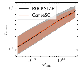
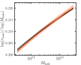
Figure 11: Various measures of the halo radius as a function of the total mass of the halo for the two halo finders CompaSO and ROCKSTAR. The left panel illustrates the radius at which the maximum circular velocity is attained, the middle panel shows the radius within which half of the halo mass is contained, and the right panel shows the recommended parameter choices which yield a measure of the virial halo radius for both halo finders.

4.5.2 Maximum circular velocity-radius

The left panel of Fig. 12 presents the maximum circular velocity versus radius at which this velocity is attained for the ROCKSTAR and CompaSO halo catalogues. The two catalogues are broadly in a good agreement, although there are differences at $V_{\rm max}\gtrsim 1000$ km/s, corresponding to the regime of low-mass clusters. The vertical line shows roughly where 100-particle haloes are located, which is the scale below which resolution effects kick in quite strongly. The CompaSO objects typically have a smaller value near $V_{\rm max}\gtrsim 1000$ km/s and a higher value for objects with $V_{\rm max}\sim 100$ km/s, which is consistent with our observation from the halo mass function (Fig. 7). In general, however, both halo catalogues show a scaling relation and $1\sigma$ scatter comparable to standard $\Lambda$CDM runs – the gray dashed curve shows the scaling relation found universally in $N$-body simulations.

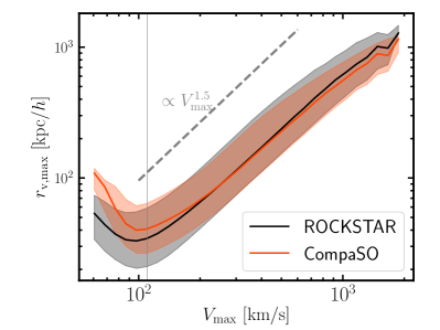
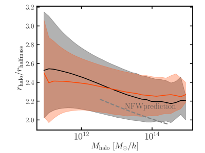
Figure 12: Left panel: relation between $V_{\rm max}$ and the radius at which it is attained. We see very good agreement between the two halo finders, with the CompaSO curve appearing a little flatter. The gray dotted line shows the typical shape found in other $N$-body simulations. Right panel: relation between the concentration proxy, $r_{\rm halo}/r_{\rm halfmass}$, and the halo mass. We see that the two curves compare well with the mass-concentration relationship appearing slightly flatter in the CompaSO case. The gray dotted line shows the NFW prediction for this ratio. The CompaSO quantity used as proxy for $r_{\rm halo}$ here is $r_{98}$, the radius containing 98% of the particles, while the ROCKSTAR $r_{\rm halo}$ proxy is the default virial radius.

4.5.3 Mass-concentration

In the right panel of Fig. 12, we visualise the mass-concentration relation in CompaSO and ROCKSTAR. As a proxy for concentration, we use the ratio $c=r_{\rm halo}/r_{\rm halfmass}$, where $r_{\rm halfmass}$ is the radius enclosing 50% of the particles and $r_{\rm halo}$ in the case of CompaSO is $r_{98}$ (the radius encompassing 98% of the particles in a halo), whereas for ROCKSTAR we use the default virial radius output as $r_{\rm halo}$. The two halo finders exhibit a very similar scatter, with the contours of CompaSO being a little tighter than ROCKSTAR, particularly at low halo mass. In addition, the low-mass CompaSO haloes appear to be less concentrated than the ROCKSTAR ones. That finding is very sensitive to the concentration proxy used to obtain the CompaSO concentrations (e.g., $c=r_{75}/r_{33}$ yields higher values), but for consistency, we are keeping the definitions across the two catalogues analogous. The results might differ depending on the halo center definition used to compute these quantities (see Fig. 10). The observed relationship between mass and concentration is similar to what is found by other $N$-body simulation codes and group finders.

5 Discussion

At heart, our new halo-finding method (CompaSO) can be thought of as an extension of the SO algorithm, and yet, its particular implementation differs quite significantly. Most notably, instead of simply truncating the haloes at the overdensity threshold as done in the standard SO algorithms, our method takes into account the tidal radii around all nearby haloes before assigning halo membership to a given particle. By adopting this approach, we aim to alleviate a traditional weakness of position-space halo finders – namely, their ability to deblend haloes. Phase-space halo finders such as ROCKSTAR (Behroozi et al., 2013) typically circumvent this issue by using 6-dimensional information about the particle distributions. For this reason, we take particular interest in the comparison between ROCKSTAR and CompaSO. Furthermore, many of the traditionally used halo finders struggle to identify haloes close to the centers of larger haloes due to the very high density of these regions. To mitigate this issue, our finder allows new haloes to form within the density threshold radius, i.e. on the outskirts of other (typically larger) haloes. In addition, we merge unphysical haloes to close companions via the cleaning procedure described in Bose et al. (2021) and summarised in Section 3. We demonstrate that the cleaning successfully removes a large number of the ill-defined haloes and leads to more “sensible” answers for some diagnostic statistics (e.g., two-point correlations). We consider other ways of identifying such objects including particle unbinding, virialisation and radial ratio tests. We find that the cleaning alone does a sufficiently good job in removing the vast majority of wrongdoers. For some particular applications, we show that combining additional halo statistics such as the virialisation ratio may help remove the remaining outliers.

In this work, we have described in detail the CompaSO halo finding method which is the default halo algorithm in the AbacusSummit suite of $N$-body simulations. We have made several parameter choices discussed in the text and extensively tested in smaller simulation boxes, such as the choice of the inner eligibility radius (set at $R_{\rm L1,elig}=80\%R_{\rm L1}$) and the Level 1 (L1) density threshold, $\Delta_{L1}$. We have also listed the various optimization and implementation techniques we employed in order to fit into the Summit allocation constraints. More details on the performance and optimization strategies are provided in the main AbacusSummit papers (Maksimova et al., 2021; Garrison et al., 2021).

To study the properties of the CompaSO haloes, we have provided a variety of comparison tests with the temporal phase-space halo-finding method ROCKSTAR, which is considered highly accurate albeit computationally expensive. We have first compared the halo mass functions derived from the CompaSO and ROCKSTAR catalogues using two different mass proxies: the virial mass of the halo and the maximum circular velocity. We have shown (see Fig. 7) that in the virial mass case, the two mass functions exhibit a slight tilt with respect to each other and that the largest differences come from the very low-mass ($\sim 10\%$, $\log(M_{\rm halo})=11$) and the very high-mass regime ($\sim 50\%$, $\log(M_{\rm halo})=15$). Repeating this comparison for the maximum circular velocity $V_{\rm max}$, we have observed that the discrepancy between the two finders is much smaller, at $\sim 5\%$ across the $V_{\rm max}$ range. This suggests that CompaSO and ROCKSTAR are finding largely the same objects in the simulation and that the difference can be attributed predominantly to the mass definitions and the drawing of halo boundaries. We have also demonstrated that our clean catalogues reconcile some of the tension with ROCKSTAR. This finding also suggests that when constructing HOD catalogues, adopting the cleaned catalogues is likely to give us a galaxy sample that is in a better agreement with ROCKSTAR. We have also shown that the CompaSO halo profiles agree reasonably well with the predictions of the NFW formalism (see Fig. 8).

The general trend corroborated by the comparison of their auto- and cross-correlation functions is that the CompaSO algorithm finds a larger number of smaller haloes on the outskirts of the largest haloes and more readily deblends these large objects. In Fig. 9 we also show that the cleaned CompaSO catalogues result in clustering that appears to be much more similar to that of the ROCKSTAR haloes. To follow up on this finding, we test the persistence of the CompaSO haloes by studying their past merger histories. A powerful diagnostic we explore is the comparison of whether a merger tree built snapshot-by-snapshot (dubbed as “fine”) yields the same progenitors for a given halo as obtained by a merger tree built across significantly longer time jumps (dubbed as “coarse”). For the haloes at $z=0.5$, we obtain a high percentage of matches at the first “coarse” time step ($z=0.875$, more than 97% for $\log(M)>10^{12.5}$) and a relatively high one at the second ($z=1.625$, close to 90%). We find that in the higher mass regime, $\log(M)>10^{12.5}$, the percentage of haloes flagged as “potential splits” is negligible ($\ll 0.1\%$). In terms of the best halo center choice, our recommendation (motivated by Fig. 10) is to use quantities computed with respect to the L2 center-of-mass (L2 com), which is both closer to the shrinking-radius center than the L1 com, and at the same time does not exhibit the issue that the L1 and L2max particle centers have of occasionally not coinciding with the location of the “true” density peak.

Overall, we have presented a highly efficient halo-finding method which provides a recipe for deblending haloes and determining particle membership on the outskirts of large haloes at a negligible computational expense compared with other accurate halo finders. While CompaSO does not currently output sufficient information about its subhaloes (L2 haloes), combining the L1 haloes with the merger tree outputs can allow us to build reliable halo catalogues, which are central to galaxy population approaches such as the HOD model. Creating highly realistic galaxy mock catalogues will be one of the biggest challenges for current cosmological efforts, and improving the accuracy of the halo finding techniques can therefore be of crucial importance for the advancement of observational large-scale structure cosmology.

Data Availability

The simulation data is available as part of AbacusSummit and is subject to the academic citations described at https://abacussummit.readthedocs.io/en/latest/citation.html.

Data access is available through OLCF’s Constellation portal. The persistent DOI describing the data release is 10.13139/OLCF/1811689. Instructions for accessing the data are given at https://abacussummit.readthedocs.io/en/latest/data-access.html.

Appendix A Mock halo tests

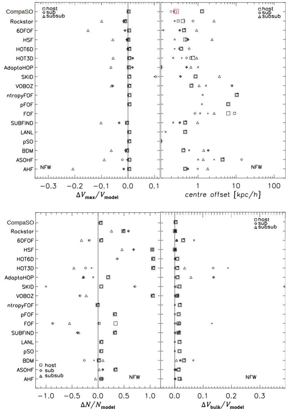
Figure 13: Recovery of various halo properties by CompaSO and other halo finders: maximum circular velocity (upper left), offset of the halo centre (upper right), number of particles (lower left), bulk velocity (lower right). Displayed are the results for only the host haloes (squares), as CompaSO does not output subhalo properties. The size of the squares indicates the test sequence (i.e. larger symbols for haloes containing more sub(sub)haloes). Adapted from Knebe et al. (2011).

All of the tests presented in the main body of this work are conducted using cosmological boxes. A useful test, therefore, is to compare the performance of CompaSO with that of other halo finders in a controlled environment. Knebe et al. (2011) offers a comparison of the halo properties retrieved by a number of different halo finders, spanning a wide range of techniques such as friends-of-friends (FOF), spherical-overdensity (SO) and phase-space based algorithms. We perform the mock halo tests provided in Knebe et al. (2011) on CompaSO. We note, however, that only a subset of these tests are relevant for CompaSO (in particular, those measuring halo properties), since it does not output any subhalo information apart from statistics with respect to the centre of the largest subhalo, which are only used to define the halo properties more robustly.

In Fig. 13, we show CompaSO alongside the other halo finders explored in Knebe et al. (2011) for three different scenarios involving NFW mock haloes: a single-halo system, a halo-subhalo system, and a halo-subhalo-subsubhalo system. We only report the host halo properties for each of these and indicate them with a square (small, medium, and large, respectively). The properties explored are maximum circular velocity ($V_{\rm max}$), offset of the halo centre, number of particles ($N$), bulk velocity ($V_{\rm bulk}$), expressed as fractional differences, $\Delta X/X_{\rm model}$, with respect to the input value, $X_{\rm model}$. For more information, see Knebe et al. (2011). We see that CompaSO recovers all four properties very well. In particular, its measurement of $V_{\rm max}$ and $N$ is among the best, outperforming nearly all phase-space finders. The recommended CompaSO proxy for the bulk velocity is v_L2com, the mean velocity of all particles in the largest subhalo. Its value depends on the subhalo density threshold, SODensityL2 (see Table 1), with higher values leading to a more accurate measure of the input bulk velocity. Finally, the recommended halo centre, defined as x_L2com, i.e. the mean position of all particles in the largest subhalo, is denoted with black squares and exhibits a similar dependence on the subhalo density threshold threshold with higher threshold values yielding less of an offset. We see that using the default threshold value yields similar results to the bulk of the halo finders. Using the particle centre of the largest L2 halo, shown in red squares, performs better, in agreement with our finding in Fig. 11.

Appendix B Parameter choices

In this appendix, we explore several of the parameter choices made in the CompaSO halo-finding algorithm. The procedure for obtaining the CompaSO halo catalogue is detailed in Section 2.2. There are several free parameters that need to be fixed when performing halo-finding using CompaSO. Here we discuss some of these choices.

B.1 Linking length, eligibility radius, density threshold

The parameters that have the most direct impact on the halo statistics such as the halo mass function and the two-point clustering are: FoFLinkingLength, L0DensityThreshold, and SO_alpha_eligible. (for definitions, see Table 1). First, we vary the modified FoF linking length of the L0 groups since it is possible that the L1 CompaSO haloes are confined by the L0 edges rather than their SO density thresholds. Similarly, we decrease the threshold on the kernel density, as the higher value that we have set might be exluding particles that would otherwise have joined L1 haloes. Finally, we study the effect of the eligibility radius, which determines the radius from the center of a given halo at which particles are eligible to form new halo nuclei. Here we perform a few tests by varying these parameters in 5 small simulation boxes: GF_N512_L150-fiducial, GF_N512_L150-alpha0.7, GF_N512_L150-alpha0.9 GF_N512_L150-b0.30 GF_N512_L150-thresh40, each with box-size $L_{\rm box}=150\ {\rm Mpc}/h$ and $N_{\rm part}=512^{3}$ particles. We note that the resolution of these boxes matches very well that of the AbacusSummit_highbase_c000_ph100 box studied in the rest of the paper. In Table 3, we specify for each of the small boxes what values we adopt for the parameters that we vary. We note that the subsequent analysis is performed on the $z=0$ snapshot.

	fiducial	alpha0.7	alpha0.9	b0.30	thresh40
BoxSize	150 Mpc$/h$	150 Mpc$/h$	150 Mpc$/h$	150 Mpc$/h$	150 Mpc$/h$
NP	$512^{3}$	$512^{3}$	$512^{3}$	$512^{3}$	$512^{3}$
ParticleMassHMsun	$2.189\times 10^{9}\ M_{\odot}/h$	$2.189\times 10^{9}\ M_{\odot}/h$	$2.189\times 10^{9}\ M_{\odot}/h$	$2.189\times 10^{9}\ M_{\odot}/h$	$2.189\times 10^{9}\ M_{\odot}/h$
FoFLinkingLength	0.25	0.25	0.25	0.30	0.25
SO_alpha_eligible	0.8	0.7	0.9	0.8	0.8
L0DensityThreshold	60	60	60	60	40

Table 3: Specifications of the small boxes (of the series GF_N512_L150) used to test the CompaSO parameter choices. See Table 1 for a more detailed description of the variables names. Here we vary the parameters that have the most direct impact on halo statistics such as the halo mass function and the two-point correlation function.

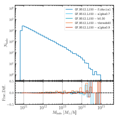
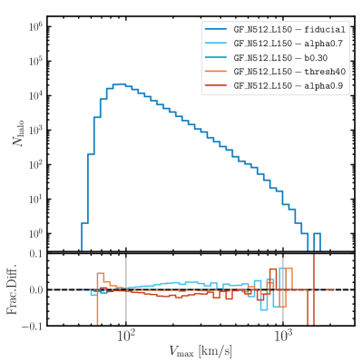
Figure 14: Halo mass functions of the CompaSO-defined groups. The upper panel shows the traditional halo mass function computed as the number of haloes as a function of halo mass for both finders, while the lower panel shows the number of haloes as a function of the maximum circular velocity $V_{\rm max}$. We see that the differences between the test boxes are quite small on all scales except for the high-mass regime in the top panel, where we have very few objects. In the bottom panel, we see that the most substantial effect on the halo function results from varying the eligibility radius parameter.

In Fig. 14, we show the halo mass functions for the 5 test boxes computed using the total halo mass ($M_{\rm halo}$) as well as the maximum circular velocity ($V_{\rm max}$) analogously to Fig. 7. In the top panel, showing the number of haloes as a function of halo mass, we see that there are negligible differences between the boxes in the small-mass regime, i.e. the fractional difference with respect to the fiducial case is less than $10\%$ for haloes of mass $M_{\rm halo}\lesssim 10^{14}\ {\rm Mpc}/h$. The difference is more pronounced for larger haloes $M_{\rm halo}\gtrsim 10^{14}\ {\rm Mpc}/h$, but noticing a trend in that regime is also more difficult since we have much fewer examples of such haloes. In the lower panel, we display the number of haloes as a function of maximum circular velocity $V_{\rm max}$. We notice that on all scales, the fractional difference with respect to the fiducial sample is less than 5%, suggesting that the halo-finding parameters have a rather small effect on the resulting halo mass function. This is reassuring to see as it shows that the CompaSO haloes are unlikely to be affected by algorithmic flaws such as hitting the edge of the L0 group when defining L1 haloes within (tested through GF_N512_L150b0.30) and having too high kernel density threshold that excludes many particles from joining L0 groups (tested through GF_N512_L150-thresh40). The most substantial effect on the halo mass function comes from varying the eligibility radius. Intuitively, setting a higher value of $R_{\rm L1,elig}$ reduces the number of substructures defined as distinct haloes on the outskirts of larger haloes, which goes in the same direction as the ROCKSTAR catalogues (see Fig. 7 in which we present the fractional difference with respect to ROCKSTAR). The opposite holds when choosing a lower value of the eligibility radius. The default value for the AbacusSummit boxes has been chosen as $R_{\rm L1,elig}=0.8\ R_{\rm L1}$ since at the boundaries of large haloes the density profile drops significantly (roughly by a factor of 5) and thus any structure that satisfies the eligibility criteria at that radius (see Section 2.2) is likely to be a not-yet-merged smaller halo in orbit around a larger object. Yes smaller values of the eligibility radius produce wedge-like gouges on the surface of large haloes.

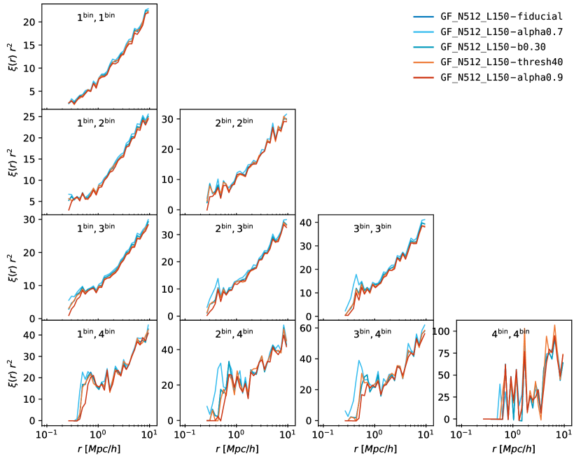
Figure 15: Two-point correlation functions of the CompaSO haloes in several smaller test boxes. The four mass bins considered in this analysis are: $1^{\rm st}\ {\rm bin}$: $\log M=12.0\pm 0.2$, $2^{\rm nd}\ {\rm bin}$: $\log M=12.5\pm 0.2$, $3^{\rm rd}\ {\rm bin}$: $\log M=13.0\pm 0.2$, $4^{\rm th}\ {\rm bin}$: $\log M=13.5\pm 0.4$, measured in $M_{\odot}/h$, and we have computed cross-correlations between each pair. We see that the curves look very similar for all parameter choices, with the largest difference being observed when varying the eligibility radius $R_{\rm L1,elig}$. A large value of $R_{\rm L1,elig}$ reduces the bump in the cross-correlations, whereas a small value produces an excess of small haloes on the outskirts of other objects which enhances the observed peaks.

In Fig. 15, we study the cross-correlations between haloes belonging to the following four mass bins: $1^{\rm st}\ {\rm bin}$: $\log M=12.0\pm 0.2$, $2^{\rm nd}\ {\rm bin}$: $\log M=12.5\pm 0.2$, $3^{\rm rd}\ {\rm bin}$: $\log M=13.0\pm 0.2$, $4^{\rm th}\ {\rm bin}$: $\log M=13.5\pm 0.4$, where the mass is measured in $M_{\odot}/h$. Similarly to the halo mass function plots, we find that most of the halo-finding parameters have little effect on the correlation functions, which is a reassuring result. The largest difference among all cases is seen again when varying the eligibility radius, $R_{\rm L1,elig}$. A large value of the eligibility radius implies more conservative identification of haloes on the outskirts of large objects, which suppresses the peak in the cross-correlations and again leads to more similar behavior to the ROCKSTAR haloes, whereas a smaller value of $R_{\rm L1,elig}$ increases the bump in the cross-correlations, suggesting an even larger excess of small objects lurking around large haloes. As argued above, the choice of the fiducial value is motivated by our desire to identify haloes in dense environments where objects are in close orbits but not yet merged. To test the “realness” of these haloes, one would need to study their merger trees. This analysis is summarised in S. Bose et al. (2020) in prep., and some basic findings are presented in Section 3.2.

B.2 Smoothing scale of the weighting kernel

In this section, we discuss the choice of smoothing scale of the weighting kernel. If we pick a larger smoothing scale, we would get a less noisy density estimate, but only high-density particles would be eligible to be part of L0 (i.e. modified FoF) groups, and we could miss lower-mass haloes. Therefore, we aim to selecting a smoothing scale that is generous to the smallest haloes and does not affect the largest ones. We note that despite using a smoothing kernel, the FoF group finding (and the density cut) will still leave orphaned particles near the boundary. Nevertheless, a smoothing kernel of the type adopted in Abacus is better than FoF at including those boundary particles, as we will show below.

The smoothed density field is related to the unsmoothed one through the smoothing function $W(r;b_{\rm kernel})=1-r^{2}/b_{\rm kernel}^{2}$, so adopting the shorthand notation $b\equiv b_{\rm kernel}$, we get:

$$\delta_{b}(\bm{r})=\frac{3}{4\pi R^{3}}\int d^{3}r^{\prime}\,W\left(|\bm{r}-\bm{r}^{\prime}|;b\right)\delta(\bm{r}^{\prime}),$$ (13)

where $\delta(\bm{r})$ is a 3-dimensional density contrast and $b$ is the smoothing scale.

First, we consider the expected particle count $\bar{N}$ and variance for a uniform background (i.e. $\delta(\bm{r})=\Delta={\rm const.}$):

$$\bar{N}=\int d^{3}r\Delta\left(1-r^{2}/b^{2}\right)=\frac{2}{5}\frac{4\pi}{3}b^{3}\Delta,$$ (14)

$${\rm Var}[N]=\int d^{3}r\Delta\left(1-r^{2}/b^{2}\right)^{2}=\frac{4}{7}\bar{N},$$ (15)

where we have assumed the particle mass to be equal to 1. We would generally like to be sensitive to density contrasts around $\Delta=60$. If $b=0.4$, then $N=6.4\pm 1.4$,which implies S/N $\approx 4.4$. Keeping that in mind, let us now study the convolution of the weighting kernel and SIS profile.

These convolutions are often more easily computed in Fourier space. The Fourier counterpart of the smoothing function is given by

$$\tilde{W}(kb)\equiv\int d^{3}r\,e^{-i\bm{k}\cdot\bm{r}}W\left(|\bm{r}|;b\right),$$ (16)

which is real for a spherical smoothing function. The smoothing kernel adopted in the Abacus simulations is a rescaled version of the Epanechnikov kernel (Epanechnikov, 1969)

$$W(r;b)=1-{r^{2}}/{b^{2}},$$ (17)

and its Fourier counterpart is

$$\tilde{W}(kb)=6\frac{4\pi b^{3}}{3}\frac{j_{2}(kb)}{(kb)^{2}}.$$ (18)

To choose the smoothing scale, we study the convolution of the kernel density estimator with a spherical isothermal sphere (SIS) profile:

$$\delta(r)=\frac{200}{3}\left(\frac{R_{\rm 200m}}{r}\right)^{2}\equiv\frac{A}{r^{2}},$$ (19)

where we have expressed the profile using the halo radius containing 200 times the mean density, $R_{\rm 200m}$. The Fourier transform of this profile is:

$$\tilde{\delta}(k)=\frac{2\pi^{2}A}{k}.$$ (20)

We perform the convolution as follows:

$$\delta_{b}(\bm{r})=\frac{3}{4\pi b^{3}}\int\frac{d^{3}k}{(2\pi)^{3}}\tilde{W}(kb)\ \tilde{\delta}(k)\ e^{-i\bm{k}\cdot\bm{r}}.$$ (21)

Performing the angular integrals and substituting the Fourier transforms of $\tilde{W}(kb)$ and $\tilde{\delta}(k)$, we arrive at:

$$\delta_{b}(\bm{r})=\int_{0}^{\infty}\frac{k^{2}dk}{(2\pi)^{2}}\ \frac{3}{2}\ \frac{j_{2}(kb)}{(kb)^{2}}\ \frac{2\pi^{2}A}{k}\ 2j_{0}(kb).$$ (22)

We can now apply relation 6.574.3 (after expressing the spherical Bessel functions, $j_{\nu}$, as normal Bessel functions, $J_{\nu}$) from Gradshteyn & Ryzhik (2007) to obtain the final result for the smoothed density field:

$$\delta_{b}(\bm{r})=\begin{cases}\frac{A}{r^{2}}\ F(1,1/2;7/2;\frac{b^{2}}{r^{2}}),&\text{if }r>b\\ 5\ \frac{A}{r^{2}}\ \frac{r^{2}}{b^{2}}\ F(1,-3/2;3/2;\frac{r^{2}}{b^{2}}),&\text{if }r<b.\end{cases}$$ (23)

In Fig. 16, we show the ratio between the smoothed field and the SIS profile. This ratio peaks around $\sim$1.45 for $r\approx 0.8b$, and at $r=b$, it is 1.25. It exceeds 1 when $r\gtrsim 0.53b$, and asymptotically approaches 1 for $r\gg b$.

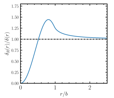
Figure 16: Ratio of the convolved SIS density profile $\rho(r)=A/r^{2}$ with the Abacus weighting kernel $W(r;b)=1-r^{2}/b^{2}$ to the SIS density profile.

Getting a sense of this behavior is very useful. If we would like to be sensitive to lower-mass haloes and have the density remain unchanged for higher-mass haloes, then we can pick a smoothing scale similar to the virial radius, $R_{\rm 200m}$, of these lower-mass haloes. That way, the smoothed density will tend to over-include particles for the smaller haloes and return to “normal” for the bigger ones. If we have a SIS with $N_{\rm 200m}=40$, that implies $R_{\rm 200m}\approx 0.36$, measured in units of the mean interparticle spacing. So using $b=0.4$ is quite well matched to our smaller haloes of $\sim$40 particles, for which S/N is around 4. Combining this with an FoF linking length of $l_{\rm FoF}=0.25$, which corresponds to $\Delta=41$, would hence render the L0 group-finding fairly complete.

We can also repeat this exercise for steeper profiles, $\rho(r)=A/r^{x}$ with $x>2$, and would find that in those cases our smoothing kernel is even more inclusive for lower-mass haloes that have $b\approx R_{\rm 200m}$.

References

- Audit et al. (1998) Audit E., Teyssier R., Alimi J.-M., 1998, A&A, 333, 779
- Barnes & Efstathiou (1987) Barnes J., Efstathiou G., 1987, ApJ, 319, 575
- Behroozi et al. (2013) Behroozi P. S., Wechsler R. H., Wu H.-Y., 2013, ApJ, 762, 109
- Bernardeau et al. (2002) Bernardeau F., Colombi S., Gaztañaga E., Scoccimarro R., 2002, Physics Reports, 367, 1
- Bertschinger & Gelb (1991) Bertschinger E., Gelb J. M., 1991, Computers in Physics, 5, 164
- Binney & Tremaine (1987) Binney J., Tremaine S., 1987, Galactic dynamics
- Bode & Ostriker (2003) Bode P., Ostriker J. P., 2003, ApJS, 145, 1
- Bond & Myers (1996) Bond J. R., Myers S. T., 1996, ApJS, 103, 41
- Bose et al. (2021) Bose S., Eisenstein D., Hadzhiyska B., Garrison L., Yuan S., Maksimova N., 2021, submitted
- Bryan & Norman (1998) Bryan G. L., Norman M. L., 1998, ApJ, 495, 80
- Bullock et al. (2001) Bullock J. S., Kolatt T. S., Sigad Y., Somerville R. S., Kravtsov A. V., Klypin A. A., Primack J. R., Dekel A., 2001, Mon. Not. R. Astron. Soc, 321, 559
- Davis et al. (1985) Davis M., Efstathiou G., Frenk C. S., White S. D. M., 1985, ApJ, 292, 371
- Dubinski et al. (2004) Dubinski J., Kim J., Park C., Humble R., 2004, New Astron., 9, 111
- Dutton & Macciò (2014) Dutton A. A., Macciò A. V., 2014, Mon. Not. R. Astron. Soc, 441, 3359
- Eisenstein & Hut (1998) Eisenstein D. J., Hut P., 1998, ApJ, 498, 137
- Epanechnikov (1969) Epanechnikov V. A., 1969, doi:https://doi.org/10.1137/1114019, 14, 153
- Evrard et al. (2002) Evrard A. E., et al., 2002, ApJ, 573, 7
- Garrison et al. (2019) Garrison L. H., Eisenstein D. J., Pinto P. A., 2019, Mon. Not. R. Astron. Soc, 485, 3370
- Garrison et al. (2021) Garrison L., Eisenstein D., Ferrer D., Maksimova N., Pinto P., 2021, submitted
- Gelb & Bertschinger (1994) Gelb J. M., Bertschinger E., 1994, ApJ, 436, 467
- Gradshteyn & Ryzhik (2007) Gradshteyn I. S., Ryzhik I. M., 2007, Table of integrals, series, and products, seventh edn. Elsevier/Academic Press, Amsterdam
- Jenkins et al. (2001) Jenkins A., Frenk C. S., White S. D. M., Colberg J. M., Cole S., Evrard A. E., Couchman H. M. P., Yoshida N., 2001, Mon. Not. R. Astron. Soc, 321, 372
- Klypin et al. (1999) Klypin A., Gottlöber S., Kravtsov A. V., Khokhlov A. M., 1999, ApJ, 516, 530
- Knebe et al. (2011) Knebe A., et al., 2011, Mon. Not. R. Astron. Soc, 415, 2293
- Knollmann & Knebe (2009) Knollmann S. R., Knebe A., 2009, ApJS, 182, 608
- Lacey & Cole (1994) Lacey C., Cole S., 1994, Mon. Not. R. Astron. Soc, 271, 676
- Lokas (2000) Lokas E. L., 2000, Mon. Not. R. Astron. Soc, 311, 423
- Maksimova et al. (2021) Maksimova N., Garrison L., Eisenstein D., Hadzhiyska B., Bose S., Satterthwaite T., 2021, submitted
- More et al. (2011) More S., Kravtsov A. V., Dalal N., Gottlöber S., 2011, ApJS, 195, 4
- Navarro et al. (1996) Navarro J. F., Frenk C. S., White S. D. M., 1996, ApJ, 462, 563
- Park (1990) Park C., 1990, Mon. Not. R. Astron. Soc, 242, 59P
- Peebles (1980) Peebles P. J. E., 1980, The large-scale structure of the universe
- Power et al. (2003) Power C., Navarro J. F., Jenkins A., Frenk C. S., White S. D. M., Springel V., Stadel J., Quinn T., 2003, Mon. Not. R. Astron. Soc, 338, 14
- Press & Schechter (1974) Press W. H., Schechter P., 1974, ApJ, 187, 425
- Sheth & Tormen (1999) Sheth R. K., Tormen G., 1999, Mon. Not. R. Astron. Soc, 308, 119
- Springel et al. (2001) Springel V., White S. D. M., Tormen G., Kauffmann G., 2001, Mon. Not. Roy. Astron. Soc., 328, 726
- Springel et al. (2005) Springel V., et al., 2005, Nature, 435, 629
- Stücker et al. (2021) Stücker J., Angulo R. E., Busch P., 2021, arXiv e-prints, p. arXiv:2107.13008
- Warren et al. (1992) Warren M. S., Quinn P. J., Salmon J. K., Zurek W. H., 1992, ApJ, 399, 405
- Warren et al. (2006) Warren M. S., Abazajian K., Holz D. E., Teodoro L., 2006, ApJ, 646, 881
- White et al. (2001) White M., Hernquist L., Springel V., 2001, ApJ, 550, L129