The impact of precession on the observed population of ULXs

Abstract

The discovery of neutron stars powering several ultraluminous X-ray sources (ULXs) raises important questions about the nature of the underlying population. In this paper we build on previous work studying simulated populations by incorporating a model where the emission originates from a precessing, geometrically beamed wind-cone, created by a super-critical inflow. We obtain estimates – independent of the prescription for the precession period of the wind – for the relative number of ULXs that are potentially visible (persistent or transient) for a range of underlying factors such as the relative abundance of black holes or neutron stars within the population, maximum precessional angle, and LMXB duty cycle. We make initial comparisons to existing data using a catalogue compiled from XMM-Newton. Finally, based on estimates for the precession period, we determine how the eROSITA all-sky survey (eRASS) will be able to constrain the underlying demographic.

1 Introduction

Ultraluminous X-ray sources (ULXs) are defined as extra-galactic, off-nuclear point sources, with inferred isotropic luminosities in excess of $L\approx 1\times 10^{39}\ \mathrm{erg}\ \mathrm{s}^{-1}$, around the Eddington limit for a typical stellar mass black hole (see Roberts 2007; Kaaret et al. 2017). Originally considered to be candidates for hosting intermediate mass black holes with sub-Eddington accretion rates (Colbert & Mushotzky, 1999), it is now accepted that most ULXs contain stellar mass black holes (BH) or neutron stars (NS) accreting at super Eddington (or ‘super-critical’) rates. To-date, there have been ten ULXs discovered to harbour neutron star accretors, eight identified through the detection of coherent pulsations (e.g. Bachetti et al. 2014; Fürst et al. 2016; Israel et al. 2017; Tsygankov et al. 2017; Doroshenko et al. 2018; Carpano et al. 2018; Sathyaprakash et al. 2019; Rodríguez Castillo et al. 2020), and one via a cyclotron resonance scattering feature (CRSF), potentially indicating the presence of strong quadrupole magnetic fields (Brightman et al. 2018; Middleton et al. 2019a; note also the potential CRSF indirectly located in NGC 300 ULX-1 by Walton et al. 2018, see also Koliopanos et al. 2019).

In the case of super-critical accretion, the accretion rate in Eddington units, $\dot{m_{0}}=\dot{m}/\dot{m}_{\rm Edd}>1$, with the accretion flow first reaching the local Eddington limit around the spherization radius at $r_{\rm sph}\approx\dot{m_{0}}r_{\rm in}$, where $r_{\rm in}$ is the inner radius of the disc, presumed to be the innermost stable circular orbit (ISCO). In the case of a magnetised neutron star, as long as $r_{\rm sph}$ is larger than the magnetospheric radius, then the Eddington limit is expected to be reached locally in the disc of both NS and BH ULXs (conversely, for very strong dipole fields, the flow will change accordingly - see Mushtukov et al. 2017a; Mushtukov 2018). At $r_{\rm sph}$, the radiation pressure inflates the disc towards scale heights of order unity (Poutanen et al., 2007). In order to stay locally below the Eddington limit, mass must be lost in the form of an outflow, which forms an optically thick wind-cone (see Poutanen et al. 2007) which can collimate the radiation from within. This ‘geometrical beaming’ of the radiation naturally leads to deviations from isotropy and a higher inferred luminosity (King et al., 2001).

Under the assumption that geometrical beaming acts to some extent across the entire ULX population (i.e. ignoring the presence of very strong magnetic fields - see King & Lasota 2019 but also Mushtukov et al. 2021a), the proportion of neutron stars and black holes within the ULX population has been analytically estimated by Middleton & King (2017), while estimates leveraging binary population synthesis have also recently been explored (Wiktorowicz et al., 2019). Both studies predict that, whilst NS systems almost certainly dominate the entire intrinsic population of ULXs, observationally the populations of NS and BH ULXs may be comparable (particularly for host regions with low metallicity), although this may be in conflict with spectral similarities between the brightest ULXs (typically $>$ a few $\times$ 10${}^{39}\ \mathrm{erg}\ \mathrm{s}^{-1}$) and those systems confirmed to harbour neutron stars (Pinto et al., 2017; Walton et al., 2018).

The light curves of several ULXs show modulations on month timescales, such as the $\sim\mathrm{62}$ and $\sim\mathrm{55}$ day periods seen in both M82 X-1 and X-2 (Kaaret et al., 2006; Kong et al., 2016), and the $\sim\mathrm{78}$ day modulation detected in NGC 5907 ULX-1 (Walton et al., 2016b). These modulations may be explained by the forced rotation of the accretion curtain in the case of a very high dipole field NS (see Mushtukov et al. 2017a) or, alternatively as suggested by Pasham & Strohmayer (2013) in the case of M82 X-1, a precessing accretion disc. The precession of an accretion disc may be driven by a variety of external torques, including tidal effects, radiation pressure driven instabilities, Lense-Thirring precession, magnetic warping and free-free precession (Fragile et al., 2007; Maloney & Begelman, 1997; Maloney et al., 1998; Pringle, 1996; Lei et al., 2013). Lense-Thirring (solid-body) precession of the large scale-height disc and wind has recently been proposed as the driving mechanism for the modulations (Middleton et al. 2018; Middleton et al. 2019b) and is somewhat compelling as it requires a misaligned spin and binary axis, the same requirement for the detection of pulsations (King & Lasota, 2020).

Under the assumption that ULXs are geometrically beamed sources with a precessing disc/wind (regardless of the mechanism), then it follows that the true population of ULXs is composed of (i) sources where we always view at low inclinations to the wind-cone such that they are persistently above the $1\times 10^{39}\ \mathrm{erg}\ \mathrm{s}^{-1}$ limit, (ii) sources where we always view at high inclinations to the wind-cone such that they are persistently below the $1\times 10^{39}\ \mathrm{erg}\ \mathrm{s}^{-1}$ limit (e.g. SS433, Fabrika 2004; Middleton et al. 2021), and (iii) sources which precess, such that the effective observer inclination transitions between (i) and (ii) (Middleton et al., 2015). In this paper we investigate the effect of geometrical beaming combined with precession on the observed population of ULXs.

The recent launch of the eROSITA mission (Cappelluti et al., 2011; Predehl et al., 2021) and the start of its all sky survey (eRASS) will enable the long-term X-ray variability of sources across the entire sky to be probed. As we will demonstrate, the rate of discovery of ULXs in eRASS monitoring may help in answering broad questions relating to the abundance of BH and NSs in the ULX population.

2 Simulation Methods

2.1 Population Synthesis

Following the work of Wiktorowicz et al. (2017) we obtained a sample of simulated binary systems using the population synthesis code StarTrack (Belczynski et al., 2008, 2020). The code simulates the evolution of binaries while accounting for all processes that can be important for the formation and evolution of ULXs such as the common envelope phase, Roche Lobe overflow (RLOF) and tidal interactions. In addition, population synthesis invokes multiple formation channels in a variety of stellar environments (metallicity, star formation history, age, etc.), and thereby provides synthetic data for comparison to observations. The code outputs comprehensive information about system parameters, which we use to calculate additional quantities required for our analysis.

2.2 Luminosity and Beaming Factor

We proceeded to select only those binary systems undergoing mass transfer from the simulated sample; this provided 104,883 unique binary systems. For each of these systems, their Eddington luminosity at each time interval was calculated using $L_{\rm Edd}=1.3\times 10^{38}m\ \mathrm{erg}\ \mathrm{s}^{-1}$ (i.e. assuming a Hydrogen composition), where $m$ is the compact object mass in solar units. The Eddington mass transfer rate was calculated from $\dot{m}_{\rm Edd}=L_{\rm Edd}/\eta c^{2}$ where we use $\eta\approx 0.08$ for both NS and BH systems. Following Shakura & Sunyaev (1973) and Poutanen et al. (2007), we obtain the intrinsic isotropic luminosity of the source without beaming $\mathrm{L_{\rm iso}}$ (and ignoring energy lost in driving a wind, or advected in the case of BHs):

$$L_{\rm iso}\approx\left\{\begin{array}[]{ll}L_{\rm Edd}[1+\mathrm{ln}(\dot{m}_{\rm 0})]&\mbox{if }\dot{m}_{\rm 0}\geq 1\\ L_{\rm Edd}\dot{m}_{\rm 0}&\mbox{otherwise}\end{array}\right.$$ (1)

Following Wiktorowicz et al. (2017), we defined the beaming factor, $b$:

$$b=\left\{\begin{array}[]{ll}1&\mbox{if }\dot{m}_{\rm 0}<8.5\\ 73/\dot{m}_{\rm 0}^{2}&\mbox{if }8.5\leq\dot{m}_{\rm 0}<150\\ 3.2\times 10^{-3}&\mbox{if }\dot{m}_{\rm 0}\geq 150\\ \end{array}\right.$$ (2)

which is related to the solid angle of the wind-cone subtending a half-apex angle $\theta/2$ by $b=1-\cos(\theta/2)$. A beaming factor of $b=1$ corresponds to no beaming and a half opening angle $\theta/2$ of $90^{\circ}$, while the smallest, limiting value of $3.2\times 10^{-3}$ corresponds to a half opening angle of $\sim 4.6^{\circ}$ (see Lasota et al. 2016). Under the assumption of an isotropic volume distribution of sources, the beaming factor $b$ is equal to the probability of observation, i.e. the probability that the beam enters our line-of-sight, which we account for in our calculations. The $b\propto 1/\dot{m}_{\rm 0}^{2}$ relation was derived by King (2009) as an extension to the treatment of black-body emission from the accretion disc around a black hole (King & Puchnarewicz, 2002), and supports the observation that several bright ULXs appear to show an anti-correlation between their peak luminosity and characteristic soft X-ray temperature (Feng & Kaaret, 2007; Kajava & Poutanen, 2009).

With values calculated for $L_{\rm iso}$ and $b$, we then obtained the maximum beamed luminosity $L_{\rm x}$ that would be observed for a given simulated system (noting the aforementioned caveats) by dividing the intrinsic luminosity by its beaming factor:

$$L_{\rm x}\approx\frac{L_{\rm iso}}{b}\\$$ (3)

We note that, in the above, we have assumed the beamed luminosity corresponds to the observed luminosity; this is an over-simplification (see the Discussion), as the true effect of beaming on the spectrum (and therefore total X-ray luminosity) requires consideration of the radial dependence of beaming (which can be substantially different for regions around the spherisation radius compared to the inner-most regions (Khan et al. in prep). We also note that the above formula assumes that the flow is ‘classically’ super-critical and therefore that the magnetic field of a neutron star in a given ULX is typically weak enough such that the magnetospheric radius is far smaller than the spherisation radius (see Mushtukov et al. 2017a for a discussion of the nature of the flow when this condition is not met) and explicitly ignores emission from the accretion column.

2.3 Duty Cycle

The disc instability model (DIM; Lasota 2001), modified for irradiation, explains the outbursts of low-mass X-ray binaries (LMXBs) as being mediated by the well-known thermal-viscous instability of an $\alpha$ disc (Shakura & Sunyaev 1973, see also Hameury & Lasota 2020 for a recent extension to higher accretion rates). The duty cycle of the resulting outbursts, $d$, is defined as the fraction of total time spent in outburst. Observationally, the value for $d$ is not particularly well constrained; extreme cases include that of GRS 1915+105 with an outburst duration exceeding 20 years and a predicted recurrence time of $\sim 10^{4}$ years, giving it an X-ray duty cycle of $\sim 0.1\%$ ($d\sim 0.001$) (Deegan et al., 2009). The Galactic LMXB, GX 339-4 on the other hand has outbursts with a recurrence time of $\sim 450$ days; based on eight outbursts provided in Rubin et al. (1998), we estimate the duty cycle to be roughly $\sim 30\%$ $(d\sim 0.3)$, whilst Chandra observations of two ULXs in NGC 5128 place an upper limit on their duty cycles of $d\sim 0.2$ (Burke et al., 2013).

In order to accommodate the observational impact of duty cycles within our parent population, we defined a sub-sample of systems undergoing nuclear timescale mass transfer that are not wind fed, and had donor stars with an effective temperature of $T_{\mathrm{eff}}<7000K$ (to be below the instability threshold, see Lasota 2001) and donor star masses below $5M_{\odot}$. For simplicity, we make the assumption that the outer regions of the disc have the same temperature as the companion star calculated via $T_{\mathrm{eff}}=({L_{\mathrm{2}}/4\pi R_{\mathrm{2}}^{2}\sigma)^{1/4}}$, where $\sigma$ is the Stefan-Boltzmann constant, and $L_{\mathrm{2}}$, and $R_{\mathrm{2}}$ are the luminosity and radius of the companion star respectively. For these systems likely to undergo outbursts mediated by the DIM, we selected a single value for $d$ such that a system with, e.g. $d=0.2$, could potentially reach ULX luminosities for 20% of its total lifetime. At gas temperatures exceeding 7000 K, we assume that the disc is constantly transporting angular momentum and does not display recurrent outbursts i.e $d=1.0$. With relevance to these latter sources, we note that we have not included the propeller effect which may act to lower the duty cycle for wind-fed or persistently accreting neutron star systems. We have also not accounted for the duty cycles of Be-X-ray binaries which undergo recurrent outbursts as a result of the neutron star’s highly elliptical orbit and passage through the decretion disc (e.g. Reig 2011).

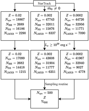
Figure 1: Flowchart showing the filtering process to obtain a representative sample population of ULXs. See section 2.4 for more detail.

2.4 Obtaining a representative population of ULXs

The impact of precession on the observed population of ULXs depends on the underlying population demographic, and thus we adopt the following method for creating representative sample populations. Figure 1 illustrates our method for generating samples of ULXs from the initial populations created via StarTrack. The simulated results are grouped into three metallicities: $Z=1\%Z_{\odot},\ 10\%Z_{\odot},\ Z_{\odot}$ (where solar metallicity, $Z_{\odot}=0.02$) and we perform simulations for each group separately as well as the combination of all three. As previously stated in section 2.2, we filtered to only include systems undergoing active mass transfer. Next, we filtered out the 16,135 binary systems that were undergoing mass transfer from a white dwarf or did not exceed $L_{x}=1\times 10^{39}\ \mathrm{erg}\ \mathrm{s}^{-1}$ at any point during their lifetime. We note that Steele et al. (2014) argue that a globular cluster ULX in NGC4472 (Maccarone et al., 2007) displays findings consistent with a white dwarf donor star (the primary being a black hole) and so it may be possible for such sources to exist, however as their evolution is dominated by dynamic processes in the cluster, the inclusion of such ULXs requires specific prescriptions beyond the scope of this work. The filtering left us with 88,748 BH/NS systems that were undergoing either nuclear or thermal timescale mass transfer and which serves as our parent ULX population. From here we split our sample into two groups depending on whether the compact object is a NS or BH. This allowed us to later specify a desired black hole percentage $\%_{\mathrm{BH}}$ within our population.

There are important differences in how long a given system may appear as a ULX, as the duration of thermal timescale mass transfer is orders of magnitude shorter than Roche lobe overflow on the nuclear timescale of the secondary (with repeat outbursts mediated by the DIM). Therefore, should we sample uniformly over all of the systems in our parent population, we would tend to over-represent short-lived ULXs. To correct for this, we apply a sampling prescription whereby the probability of selecting a given ULX is set by its lifetime as a ULX, divided by the summed lifetime of all the other systems in the parent population $P_{\mathrm{sample}}=t_{\mathrm{ULX,n}}/\sum_{n=0}^{N_{\mathrm{ulx}}}t_{\mathrm{ULX,n}}$. This sampling procedure explicitly assumes that there exists a constant star formation rate across cosmic time.

In the following simulations, we have chosen to re-sample the total population to produce smaller, volume-limited populations of $N_{\rm sys}=500$ systems (for each metallicity); this is a little larger than the currently observed number of ULXs by XMM-Newton (Earnshaw et al., 2019) although through repeat re-sampling (our Monte-Carlo procedure), the results can be scaled to any desired population size.

2.5 Simulating ULX light curves

In order to investigate the impact of precession on the observed population of ULXs, we require a method for creating long term light curves for our synthesised population. ULXLC  is a numerical model developed by Dauser et al. (2017), to describe the luminosity emerging from within an optically thick wind-cone of half-opening angle $\theta/2$, with an observer inclination, $i$, and an outflow velocity (which also imparts some Doppler boosting) of the outflow, $\beta_{\mathrm{wind}}$ (and which hereafter we fix to $0.3c$ to be broadly consistent with the winds detected in ULXs and SS433: Middleton et al. 2014; Walton et al. 2016a; Pinto et al. 2016; Pinto et al. 2017; Kosec et al. 2018a; Kosec et al. 2018b; Middleton et al. 2021).

ULXLC also incorporates the effect of precession through a half precessional angle $\Delta i$ and precession period $P$, which may be shifted by a phase offset $\phi$. The model does not assume any physical mechanism for driving the precession and so can be used without any additional a-priori assumptions. In order to use ULXLC, we require input model parameters; $\theta$ can be derived from the assumed relationship between accretion rate, beaming and opening angle (Section 2.2), whilst $\cos i$ is uniformly distributed between zero and one, which ensures the random distribution of ULX orientations in space. $\Delta i$ is an unknown, although if we assume SS433 to be a reasonable indicator, values of $20^{\circ}$ are not implausible (Fabian & Rees, 1979; Milgrom, 1979; Margon et al., 1979). Using ULXLC, we simulated light curves for each ULX system, which took the form of a single precession cycle and a time series of 5000 data points.

The light curves from ULXLC required normalising to produce physical luminosity units. For any given combination of system parameters (i.e. our simulated population of ULXs), we simulated a light curve at zero inclination and set the maximum luminosity to be equal to the beamed luminosity given in equation 3. This allowed us to calculate a scaling constant which we used to renormalise any light curve at arbitrary inclination and obtain a luminosity in physical units.

The light curves produced by ULXLC are periodic even though in reality precession may be quasi-periodic if dependent on accretion rate (e.g. Middleton et al. 2019b). Although the period is not utilised until we consider the regular observations taken by eROSITA (section 3.3.2), at the point of creating the light curves, we also scale the period using formulae for Lense-Thirring precession (Middleton et al., 2019b) and an empirical-only relationship (Townsend & Charles, 2020) (see equations 4 & 7).

2.5.1 Lense-Thirring Precession

Lense-Thirring precession is a relativistic correction to the precession of a gyroscope near a large rotating mass. This effect has been shown to occur in the weak-field limit around the Earth by the Gravity Probe B experiment (Everitt et al. 2011) and is believed to explain the type C quasi-periodic oscillations in black hole binaries (Stella & Vietri, 1998; Ingram & Done, 2012a, b; Ingram et al., 2017; Motta et al., 2018). The effect occurs when orbiting fluid is displaced vertically from a rotating body’s equatorial axis such that frame-dragging then induces oscillations about the ecliptic and periapsis. General relativistic magnetohydrodynamic (GRMHD) simulations of tilted accretion discs around Kerr black holes (Fragile et al. 2007) display global solid body precession of the hot inner flow, and in ULXs it is speculated that the same effect may lead to precession of the large scale-height disc and wind cone (Middleton et al. 2018; Middleton et al. 2019b).

Following Middleton et al. (2019b), we calculated the precession period of the wind-cone via equation 4:

$$P_{\rm wind}=\frac{GM\pi}{3c^{3}a_{*}}r_{\rm out}^{3}\left[\frac{1-\left(\frac{r_{\rm in}}{r_{\rm out}}\right)^{3}}{\textup{ln}\left(\frac{r_{\rm out}}{r_{\rm in}}\right)}\right]$$ (4)

We make the simplifying assumption that $r_{\rm in}=r_{\rm isco}$ in units of the gravitational radius ($GM/c^{2}$), i.e. ignoring the role of magnetic fields (although see Vasilopoulos et al. 2019 and Middleton et al. 2019b for a discussion). We assume that neutron stars are low spin ($a_{*}=0.01,\ r_{\rm isco}=6\ R_{g}$) as indicated by observations of pulsar ULXs (PULXs) to-date, with spin periods of 1-10s of seconds (King & Lasota, 2020), and that black holes may have very high spins ($a_{*}=0.998,\ r_{\rm isco}=1.25\ R_{g}$) as a consequence of the high accretion rates, the ability to advect matter and angular momentum, and the lack of a propeller mechanism to limit the spin-up. In the above, $r_{\rm out}$ is the outer photospheric radius of the wind (the point at which radiation can free-stream) for which we assume (Poutanen et al., 2007):

$$r_{\rm out}\approx\frac{3\epsilon_{\rm wind}}{\beta\zeta}\dot{m_{\rm 0}}^{3/2}r_{\rm isco}$$ (5)

where – for the purposes of determining this radius – we have assumed $r_{\rm isco}=6R_{g}$ for both NS and BHs (and an accretion efficiency of 0.08). Note that the discrepancy between assuming a high BH spin for the precession period and a larger ISCO radius here does not have a substantial effect on the location of the photosphere for large accretion rates (see Middleton et al. 2019b for details). In the above, $\beta$ is the ratio of asymptotic wind velocity relative to the Keplerian velocity at $r_{\rm sph}$, and, for simplicity, we set this to $1.4$. $\epsilon_{\rm wind}=L_{\rm wind}/L_{\rm tot}$ is the fraction of dissipated energy used to launch the wind, which we set to $\epsilon_{\rm wind}=0.25$ (Jiang et al. 2014, see also Pinto et al. 2016 for a higher inferred value from observation). Finally, $\zeta$ is the cotangent of the opening angle of the wind cone which we assume is equal to:

$$\zeta=\mathrm{tan}\left[\frac{\pi}{2}-\mathrm{acos}\left(1-b\right)\right]$$ (6)

We assume a lower-limit of $\zeta=2$ based on radiative magnetohydrodynamic simulations at moderate super-Eddington rates (Sądowski et al. 2014, and noting that in reality, $\zeta$ – and therefore $b$ – likely increases in a more complicated fashion with $\dot{m_{\rm 0}}$: Jiang et al. 2019).

2.5.2 Empirical Precession

In addition to the above physical precession mechanism, we also utilise the result of Townsend & Charles (2020), where the mechanism for precession is unknown but the super-orbital (P_sup) and orbital periods (P_orb) are inferred to be related by:

$$P_{\rm sup}=22.9\pm 0.1P_{\rm orb}$$ (7)

where P_orb is given by:

$$P_{\rm orb}=2\pi\sqrt{\frac{a^{3}}{G(M_{\rm c}+M)}}$$ (8)

where $M_{\rm c}$ is the mass of the companion star and $a$ is the semi-major axis of the binary system.

2.6 Effects of precession on the observed population of ULXs

As we mention above, in order to explore the impact of various key parameters on our observations of ULXs, we re-sample the parent population 10,000 times, each time producing a smaller sample of 500 ULXs. For each ULX in our smaller sample, we provided the following parameters to ulxlc: $\theta/2$, $i$, $\Delta i$, $L_{\rm x}$, $P$, $\phi$, $\beta_{\mathrm{wind}}=0.3$. $\Delta i$ and $\phi$ are sampled from uniform distributions with the following ranges: $0^{\circ}\leq\Delta i\leq\Delta i_{\mathrm{max}}$, $0\leq\phi\leq 1$. $\cos i$ is uniformly distributed between zero and one, $\theta/2$, whilst $L_{x}$ and $P$ are calculated quantities of the particular system. We explore the impact of $\Delta i_{\mathrm{max}}$ = $45^{\circ}$ and $20^{\circ}$, as we do not have strong constraints on the precessional angle (other than for SS433). We then proceeded to classify each light curve in our sample, created using ulxlc, into one of three categories:

• Alive: Persistently above $1\times 10^{39}\ \mathrm{erg}\ \mathrm{s}^{-1}$

• Transient: Systems that crossed $1\times 10^{39}\ \mathrm{erg}\ \mathrm{s}^{-1}$

• Hidden: Persistently below $1\times 10^{39}\ \mathrm{erg}\ \mathrm{s}^{-1}$

We note that this act of classifying sources is independent of the precession period, with systems merely being defined based on the above, regardless of the timescales involved. The numbers of systems in each classification were recorded and saved such that the total number of systems ($N_{\rm sys}$ = 500) = the number alive ($N_{\rm A}$) + the number of transients ($N_{\rm T}$) + the number of hidden systems ($N_{\rm Hid}$). Light curves that were classified as transient were subjected to further analysis (see Section 2.8.1), whilst ULX systems with half opening angles of $\theta/2>45^{\circ}$ (set by the accretion rate – see equation 2) were considered to be sources that do not display precession (see Dauser et al. 2017) and thus were classified as being alive without the need to simulate light curves.

2.7 Simulations of the X-ray Luminosity Function

X-ray luminosity functions (XLFs) – both in their differential and cumulative forms – have been commonly extracted from survey data in order to study population demographics (Fabbiano, 1989; Grimm et al., 2003; Wang et al., 2016). XLFs can provide insights into the star-formation history (Fragos et al., 2013a; Fragos et al., 2013b) and impose constraints on theoretical models of binary evolution. It is important to consider how the combination of precession and geometrical beaming can together affect the overall shape of observed XLFs. To this end we explored how a synthetic XLF would appear under six different scenarios that could describe a given source’s luminosity:

• $L_{\mathrm{iso}}$: the isotropic luminosity obtained in the absence of beaming (eq. 1)

• $L_{\mathrm{x}}$: the above including geometrical beaming (eq. 3)

• $L_{\mathrm{x,b}}$: the above including the probability of observation set by the beaming factor (i.e. assuming obscuration by the wind)

• $L_{\mathrm{x,b*d}}$: the above including the additional effect of the LMXB duty cycle on the observation probability

• $L_{\mathrm{x,prec}}$: the luminosity obtained via the generation and uniform sampling of light curves produced by ULXLC (sec. 2.5)

• $L_{\mathrm{prec,vis}}$: the above including the additional effect of the LMXB duty cycle.

As described in section 2.2, we re-sampled $N_{\rm sys}=500$ binaries from across all metallicites from our full parent population weighted by their lifetimes in the active mass transfer phase (top row in Figure 1), while specifying a black hole percentage of $\%_{\mathrm{BH}}=0,\ 50\%$ & $100\%$. For the construction of our XLFs, we separate the BHs, NSs, and LMXBs, as well as those defined as alive or transient; this is useful for illustrating the relative contributions of each component to the XLF.

LMXB sources were set to have a duty cycle of $d=0.2$ so that there was a 20% chance of them being observed at their luminosity given by $L_{\mathrm{x}}$, and an 80% chance of them not being observed at all (i.e. $L_{\mathrm{x}}=0$). Thermal timescale or wind-fed systems in our population were set to have a duty cycle of $d=1.0$. For each system (with $\theta/2<45^{\circ}$) a light curve was then generated using ULXLC assuming a precessional angle uniformly sampled between $0$ and $\Delta i_{\mathrm{max}}=45^{\circ}$; we then randomly sampled the system’s light curve to obtain its new luminosity. Re-sampling the parent population (as described in section 2.4), then allows us to obtain 1$\sigma$ errors on each luminosity bin for any given XLF.

2.8 Simulating eRASS’s view of the ULX population

The eROSITA X-ray telescope was launched in July 2019 and has already begun its all-sky survey, eRASS, which takes snapshots of the entire sky in the $0.2-10\ \mathrm{keV}$ band, repeating every six months for a period of four years (Merloni et al., 2012). Using the generated light curves for our artificial population of ULXs, we can obtain predictions for what eROSITA might observe given an underlying population demographic, and explore how our constraints might improve over the course of the eRASS four year survey.

Whilst the previous sections had no requirement to use the periods given by equations 4 & 7, given eRASS’s regular observations it is important to factor in the deterministic nature of such a periodic (or, in reality quasi-periodic – Middleton et al. 2019b) modulation of the luminosity.

We note that our simulations make the assumption that all the systems in our parent population have an equal probability of observation regardless of their spatial distribution, luminosity or spectra. In reality, there will be a natural bias towards detecting the brighter sources, which is further compounded by the anisotropic sensitivity of eRASS (with greater effective exposure occurring near the ecliptic poles and deeper coverage between 0.2 - 2.3  keV, Predehl et al. 2020). To obtain a more realistic picture requires the distribution of simulated binaries amongst galaxies out to a few 10s of Mpc, some estimate for the true number per galaxy type (and per unit star formation), their spectra and the convolution of the exposure time and detector response. Whilst this is beyond the scope of this work, we discuss the impact of resulting bias in the Discussion section.

2.8.1 eRASS Sampling Routine

The light curves that were created in Section 2.6, were scaled to have a period of both $P_{\rm wind}$ and $P_{\rm sup}$ and their luminosity was then sampled in intervals of six months to match the observing cadence of eRASS. At each eRASS cycle $(c)$, we keep track of the following:

• Sources above $1\times 10^{39}\ \mathrm{erg}\ \mathrm{s}^{-1}$, $N_{\rm ulx}(c)$

• Sources below $1\times 10^{39}\ \mathrm{erg}\ \mathrm{s}^{-1}$, $\lnot N_{\rm ulx}(c)$

• Newly detected ULXs, $N_{\rm new}(c)$

• Previously detected ULXs that fell below the ULX threshold, $N_{\rm dip}(c)$

• The change in the number of ULXs $\Delta N_{\rm ulx}(c)=N_{\rm new}(c)-N_{\rm dip}(c)$

• The number of transient sources, $N_{\rm T}(c)=N_{\rm new}(c)+N_{\rm dip}(c)$ (for $c>1$)

• The number of alive sources, $N_{\rm A}(c)$

The above quantities are naturally cycle-specific and the cumulative equivalents for these quantities may be obtained by summing over all eRASS cycles, e.g. we define the cumulative number of observed sources by $N_{\rm obs}(c)=\sum_{c=1}^{8}N_{\rm new}(c)$. We also note that the quantity $N_{\rm A}(c)$ includes the $N_{\rm A}$ systems classified as alive, with opening angles $\theta/2>45^{\circ}$, and for which light curves were not simulated (see section section 2.6).

Over the first 6 months of eRASS (cycle 1), we make the assumption that the survey will not detect any transient sources due to precession, as the exposure time is very short relative to the typical precession timescale. At the conclusion of cycle 1 we therefore have a starting value for the total number of observed ULXs which will subsequently increase as the survey continues.

We performed 10,000 sets of Monte Carlo simulations for a given combination of input parameters which covered $Z$ (0.02, 0.002, 0.0002 and the combination of all three), $\%_{\rm{BH}}$ (0 $\rightarrow$ 100 % in steps of 25%), $\Delta i_{\rm{max}}$ (20^∘ and 45^∘), P ($P_{\rm{wind}}$ and $P_{\rm{sup}}$) and d (0.2 and 1.0). At each eRASS cycle we recorded quantities which may be compared to actual eRASS  measurements, such as the number of sources detected in a given eRASS  cycle $N_{\rm ulx}(c)$. The repeat simulations allowed the construction of distributions from which we extracted the key statistics related to the various quantities in each cycle as a function of our physical parameters (notably $\%_{\rm BH}$).

An example set of results from a single Monte-Carlo iteration is shown in Table 1.

c	$N_{\rm new}(c)$	$N_{\rm dip}(c)$	$\Delta N_{\rm ulx}(c)$	$N_{\rm T}(c)$	$\sum_{c=1}^{8}N_{\rm A}(c)$	$N_{\rm obs}(c)$
1	303	0	+303	0	303	303
2	24	12	+12	36	291	327
3	8	4	+4	12	287	335
4	3	0	+3	3	287	338
5	2	2	0	4	285	340
6	1	0	+1	1	285	341
7	1	2	-1	3	283	342
8	2	0	+2	2	283	344

Table 1: An example of a single eRASS Monte-Carlo iteration showing a subset of observed quantities, created from an underlying population of $N_{\rm sys}=500$ ULXs with $\%_{\rm BH}=50$, $\Delta i_{max}=20^{\circ}$, $Z=0.02$ and $d=1.0$. The numbers illustrate the evolution of the observed population as seen by eRASS over its 8 cycles.

3 Results

3.1 The Impact of Precession on the XLF

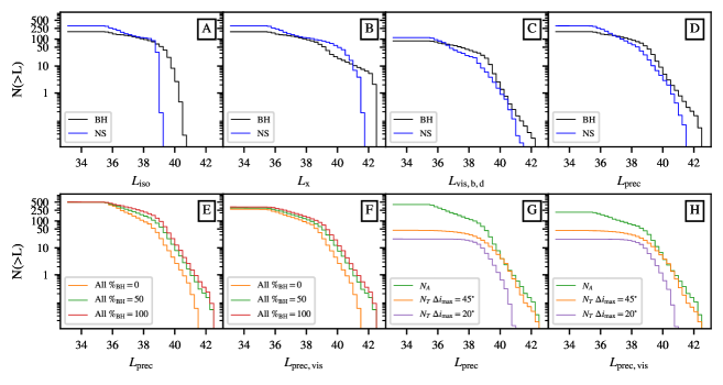
Figure 2: Cumulative XLFs shown for a variety of luminosity prescriptions. A: the XLF for BHs and NSs when assumed to emit isotropically ($L_{\rm iso}$). B: the same for beamed emission ($L_{\rm x}$). C: The same but factoring in the observation probability from beaming and LMXB duty cycle (but without precession: $L_{\mathrm{vis,b,d}}$). D: the XLF after incorporating the probability obtained from precession $L_{\mathrm{prec}}$. (see section 3.1.1). E: $L_{\mathrm{prec}}$ for different $\%_{\mathrm{BH}}$. F: The XLF incorporating precession and the addition of a LMXB duty cycle ($L_{\mathrm{prec,vis}}$). G: The XLF incorporating precession split into the classifications described in section 2.6. H: The XLF incorporating precession and duty cycle split into the classifications described in section 2.6. ($L_{\mathrm{prec,vis}}$). The first four and last two panels assume $\%_{\mathrm{BH}}=50$, while the estimates for the impact of precession assume a maximum precessional angle of $\Delta i_{\mathrm{max}}=45^{\circ}$ unless otherwise stated. Where we have included its effect, the LMXB duty cycle was set to $d=0.2$. The XLF obtained via sampling from the ULX catalogue of Earnshaw et al. (2019) is shown in cyan. The method for the creation of this plot is detailed in Section 2.7.

Following the method detailed in Section 2.7, Figure 2 shows several of our synthetic cumulative XLFs, created using the method described in section 2.4. We now use the total lifetime of the source during active mass transfer as opposed to the lifetime of the source during only the ULX phase, so that the sampling probability is given by $P_{\mathrm{sample}}=t_{\mathrm{mt,n}}/\sum_{n=0}^{N}t_{\mathrm{mt,n}}$, where $t_{\mathrm{mt,n}}$ is the amount of time spent undergoing active mass transfer for the nth source, and $N$ is the number of sources in the population.

Panel A shows an XLF assuming $\%_{\rm{BH}}$ = 50% and isotropic emission in the absence of any geometrical beaming, with no neutron stars exceeding the $1\times 10^{39}\ \mathrm{erg}\ \mathrm{s}^{-1}$ luminosity threshold (as the beaming only begins at a NS luminosity around 6 $\times$ 10${}^{38}\ \mathrm{erg}\ \mathrm{s}^{-1}$), and a few BHs reaching up to $\sim 10^{40}\ \mathrm{erg}\ \mathrm{s}^{-1}$.

Panel B (also for $\%_{\rm{BH}}$ = 50%) shows the same XLF as in Panel A after incorporating beaming but does not account for the observation probability (i.e. it assumes every detected source is observed directly down the wind cone). We see that, between $10^{38}$ and $\sim 10^{41}\ \mathrm{erg}\ \mathrm{s}^{-1}$, NSs appears to dominate, while at the highest luminosities, $>10^{41}\ \mathrm{erg}\ \mathrm{s}^{-1}$, BH accretors dominate.

Panel C includes the observation probability provided by the beaming factor $b$, and the LMXB duty cycle $d$; we see that the brightest sources above $\sim 10^{40}\ \mathrm{erg}\ \mathrm{s}^{-1}$ are suppressed and are no longer visible.

Panel D (also for $\%_{\rm{BH}}$ = 50%) includes the combined effects of geometrical beaming, precession (via ULXLC) and a LMXB duty cycle of $d=0.2$; both NS and BH systems are observed in similar numbers across the full range of luminosities, with none detected above $\sim 10^{41}\ \mathrm{erg}\ \mathrm{s}^{-1}$.

Panels E and F are created following the same process as panel D and show the XLF with and without the addition of the LMXB duty cycle respectively. Here we have combined the NS and BH populations into a single observed population and varied $\%_{\rm BH}$. We observe that the general shape of the XLF is not strongly affected by the underlying $\%_{\rm BH}$, however, for a higher proportion of BHs in the underlying population, there are a larger number of detected systems across all luminosities (with systems still being detected at a few $\times 10^{41}\ \mathrm{erg}\ \mathrm{s}^{-1}$).

Panels G and H show the same as panels E and F except we have now split the XLF into the classifications of alive and transient, with results shown for different maximum precessional angles as described in section 2.6.

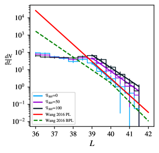
Figure 3: Several realisations of our synthetic, differential XLFs (showing $L_{\mathrm{prec}}$), for different black hole ratios: $\%_{\mathrm{BH}}=0$ (cyan), 50 (magneta) and 100 (black) and a maximum precessional angle of $\Delta i_{\mathrm{max}}=45^{\circ}$. Best fit models (both broken and unbroken power-law) from (Wang et al., 2016) are overlaid for comparison.

3.1.1 Modelling the XLF

The differential forms of observed XLFs $(dN/dL)$ are often fitted with power-laws, or variants such as broken or exponential cutoff power-laws (see Grimm et al. 2003; Swartz et al. 2011; Mineo et al. 2012; Wang et al. 2016; Wolter et al. 2018; Kovlakas et al. 2020). In Figure 3 we plot a subset of the differential forms of our synthetic XLFs versus the best fit models from Wang et al. (2016) who used Chandra observations of 343 galaxies (totalling 4970 sources, 218 of which are ULXs) to create differential XLFs. Whilst there appears to be agreement at higher luminosities $(L>10^{39})$, at lower luminosities our XLFs appear to flatten off which is inconsistent with the models based on observation; this is likely due to the excluded systems from our sampling which emit at lower luminosities (e.g. white dwarf accretors). In order to make a fair, quantitative comparison to reported slopes in the literature, we therefore model only the high luminosity tail ($>$ 10${}^{39}\ \mathrm{erg}\ \mathrm{s}^{-1}$) of the differential form of our synthetic XLFs.

Our differential luminosity functions obtained via $L_{\mathrm{\rm prec}}$ and $L_{\mathrm{\rm prec,vis}}$ are fitted using a power-law of the form $dN/dL=AL^{-\alpha}$ via a method of maximum likelihood (for limitations on this method see Clauset et al. 2007) where the errors on each bin are the standard deviation (rather than standard error which are considerably less representative in this case). Table 2 reports the corresponding best fit parameters and their 1$\sigma$ errors.

L	$\Delta i_{\mathrm{max}}$	$\%_{\mathrm{BH}}$	$A$	$\alpha$
$L_{\mathrm{prec}}$	45	0	24.60 $\pm$ 0.77	0.94 $\pm$ 0.03
$L_{\mathrm{prec}}$	45	25	36.18 $\pm$ 1.71	0.81 $\pm$ 0.03
$L_{\mathrm{prec}}$	45	50	47.16 $\pm$ 3.00	0.76 $\pm$ 0.04
$L_{\mathrm{prec}}$	45	75	59.23 $\pm$ 4.56	0.74 $\pm$ 0.05
$L_{\mathrm{prec}}$	45	100	70.40 $\pm$ 6.13	0.73 $\pm$ 0.06
$L_{\mathrm{prec}}$	20	0	23.95 $\pm$ 0.45	1.06 $\pm$ 0.02
$L_{\mathrm{prec}}$	20	25	35.61 $\pm$ 1.79	0.88 $\pm$ 0.04
$L_{\mathrm{prec}}$	20	50	47.36 $\pm$ 3.38	0.83 $\pm$ 0.05
$L_{\mathrm{prec}}$	20	75	59.86 $\pm$ 5.53	0.79 $\pm$ 0.06
$L_{\mathrm{prec}}$	20	100	71.20 $\pm$ 7.33	0.78 $\pm$ 0.07
$L_{\mathrm{prec,vis}}$	45	0	24.24 $\pm$ 0.76	0.93 $\pm$ 0.03
$L_{\mathrm{prec,vis}}$	45	25	29.28 $\pm$ 1.42	0.77 $\pm$ 0.03
$L_{\mathrm{prec,vis}}$	45	50	34.06 $\pm$ 2.34	0.70 $\pm$ 0.04
$L_{\mathrm{prec,vis}}$	45	75	39.61 $\pm$ 3.43	0.66 $\pm$ 0.05
$L_{\mathrm{prec,vis}}$	45	100	44.44 $\pm$ 4.64	0.64 $\pm$ 0.06
$L_{\mathrm{prec,vis}}$	20	0	23.60 $\pm$ 0.44	1.06 $\pm$ 0.02
$L_{\mathrm{prec,vis}}$	20	25	28.63 $\pm$ 1.26	0.84 $\pm$ 0.03
$L_{\mathrm{prec,vis}}$	20	50	34.19 $\pm$ 2.58	0.77 $\pm$ 0.05
$L_{\mathrm{prec,vis}}$	20	75	39.98 $\pm$ 3.95	0.72 $\pm$ 0.06
$L_{\mathrm{prec,vis}}$	20	100	44.96 $\pm$ 5.39	0.69 $\pm$ 0.07

Table 2: Best fit parameters and 1$\sigma$ errors from modelling our synthetic, differential XLFs above $10^{39}$ erg/s using a power law of the form $AL^{-\alpha}$.

As can be seen from Table 2, we observe a slight flattening of the XLF slope with increasing $\%_{\mathrm{BH}}$ with slightly steeper slopes found for $\Delta i_{\mathrm{max}}=20^{\circ}$ when compared to $\Delta i_{\mathrm{max}}=45^{\circ}$. The effect of the duty cycle is to lower the maximum height reached by the XLF (i.e. the total number of sources, see bottom row in Figure 2) which flattens the slope, especially when the population is BH dominated and thus extends to higher luminosities.

The existing literature contains a great deal of variation in the normalisation when fitting functional forms to XLFs. However the slopes of our synthetic differential XLFs ($\alpha$) are found to be somewhat flatter than those found in (Grimm et al., 2003) (created from HMXBs in five different galaxies), with an observed slope of $\alpha=1.61\pm 0.12$, in (Swartz et al., 2011) (using observations of 127 nearby galaxies) with an observed slope of $\alpha=1.4\pm 0.2$ above $10^{39}\mathrm{erg}\ \mathrm{s}^{-1}$, and in (Wang et al., 2016) who applied a broken power-law (with a break at $L_{b}=2.5\times 10^{38}\ \mathrm{erg}\ \mathrm{s}^{-1}$), finding the slope above the break to be $\alpha_{2}=1.1\pm 0.02$. We discuss the impact of observational bias as the likely reason for this difference in the Discussion section.

3.2 Dependence of Light Curve Classifications on Model Parameters

Following from our simulations and the placing of sources into the three categories described in Section 2.6, we now describe how the underlying nature of the population might affect our observations of ULXs.

Figure 4 shows the distributions for the number of our three light curve classifications, as well as the percentage of transient to total observable $N_{\rm T}/(N_{\rm A}+N_{\rm T})$ systems. The results are presented as a corner plot (Foreman-Mackey et al., 2021) over a subset grid of simulation parameters (see section 2.6). The two distinct regions of parameter space in Figure 4 denoted by dotted and solid contours arise from the two different maximum precessional angles, $\Delta i_{\mathrm{max}}$ $20^{\circ}$ (dotted) & $45^{\circ}$ (solid). There is considerable overlap in the number of alive and hidden systems from populations drawn when using a maximum precessional angle of $20^{\circ}$ when compared to $45^{\circ}$. However the error contours describing the number of transient sources, $N_{\rm T}$, overlap less, with smaller maximum precessional angles (up to $20^{\circ}$) resulting in fewer transient sources by around a factor two when compared to the larger maximum precessional angle (up to $45^{\circ}$). The darker regions in Figure 4 correspond to populations drawn with higher fractional abundances of BHs, while blue-er regions correspond to populations with a higher abundance of NSs. We observe that the number of hidden and transient sources, $N_{\rm Hid}$ and $N_{\rm T}$, are negatively correlated with increasing black hole percentage, while the number of alive systems increases with increasing $\%_{\mathrm{BH}}$, this trend is observed across all of our simulated metallicities, maximum precessional angles and simulated duty cycles. The latter observation follows naturally from the expectation that NS ULXs are beamed (under our assumptions which do not factor in the emission from the column nor the effects of strong dipole fields) and, combined with precession, are more likely to be observed as transient or hidden. We note that, in the absence of a LMXB duty cycle (i.e. $d=1.0$), the correlation between the number of transient sources and black hole percentage is markedly less pronounced, this is due to our prescription for LMXB systems (section 2.3) resulting in a higher number of black hole systems displaying outburst duty cycles when compared to NS systems.

In terms of the most extreme scenarios, from Figure 4 we can see that for a population composed entirely of neutron stars, around $\sim 40-50\%$ of the observable sources are defined as being transient for $\Delta i_{\mathrm{max}}=20^{\circ}$, or $\sim 60-75\%$ for $\Delta i_{\mathrm{max}}=45^{\circ}$. Conversely, for an underlying population composed entirely of black holes, the proportion of sources being defined as transient is $\sim 10-25\%$ for $\Delta i_{\mathrm{max}}=20^{\circ}$ or $\sim 30-45\%$ for $\Delta i_{\mathrm{max}}=45^{\circ}$.

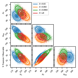
Figure 5: 2D 1$\sigma$ error contours for the distributions of light curve classifications for different parent population metallicities, $Z=0.02$ (blue), $Z=0.002$ (orange), $Z=0.0002$ (green) and the combination of all three (red) for fixed parameters: $\Delta i_{\mathrm{max}}=20^{\circ}$, $d=0.2$, $\%_{\mathrm{BH}}=50$.

The effect of changing the parent population’s metallicity, $Z$, which is shown for a fixed set of model parameters in Figure 5, does have an impact on the absolute numbers of each classification, however, the general trends previously described hold true for all metallicities and their combination.

3.3 Comparison to observations

From Figure 4 we deduce that the black hole percentage in the underlying population, and maximum precessional angle, substantially affects the percentage of transient to observed sources. This implies that, with constraints on the maximum precessional angle and suitable coverage (both in terms of area observed and cadence), it may be possible to constrain the ratio of BHs to NSs in the underlying population simply by determining the ratio of transient to alive systems (under the assumption that the variability is driven by precession and the beaming is highly sensitive to accretion rate – see the Discussion).

In the following sections we discuss initial constraints from XMM-Newton and then discuss implications for eROSITA and eRASS.

3.3.1 Constraints from XMM-Newton

To obtain some initial observational constraints on the number of alive and transient ULXs, we used the catalogue of 1314 X-ray sources compiled by Earnshaw et al. (2019), created from the 3XMM-DR4 data release of the XMM-Newton Serendipitous Source Catalogue (Rosen et al., 2016). The catalogue identifies 384 candidate ULXs, 81 of which were observed more than once. Each entry within the catalogue includes a full band (0.2 - 12 keV) apparent (absorbed) luminosity and associated $1\sigma$ errors. From the 81 ULXs with multiple observations, we sampled the luminosity (i.e. using their associated errors) 100,000 times, and separated these systems into alive or transient based on our previous definitions, and calculated associated $1\sigma$ error intervals on the respective distributions. We find that $81\pm 12\%$ of the systems may be classified as alive, while $19\pm 3.8\%$ may be classified as transient; by comparison to our simulated results, we can thereby obtain a crude estimate of the underlying, intrinsic properties of the observed population. The region denoted by the red lines on Figure 4 indicates the 1$\sigma$ interval for the percentage of transient to observed sources obtained from Earnshaw et al. (2019) and implies abundances of BHs of around 75-100% (assuming $\Delta i_{\mathrm{max}}=45^{\circ}$ or $10-100\%$ (for $\Delta i_{\rm max}\leq 20^{\circ}$), see Figure 4). As the ULXs in the Earnshaw et al. (2019) catalogue have only been observed 2-3 times, there is an observational bias towards alive systems and we underestimate the true number of transients. The inferred percentage of transient to observed systems is therefore only a lower limit and, as more transients are located, the upper limit on $\%_{\mathrm{BH}}$ we would infer from Figure 4 will steadily push to smaller values.

We also note that the luminosities obtained via sampling the observed population of Earnshaw et al. (2019) are subject to interstellar absorption, whilst the luminosities obtained from our simulations do not account for this effect. As such our results are most valid for observations made out of the Galactic plane and of other galaxies viewed at low inclinations.

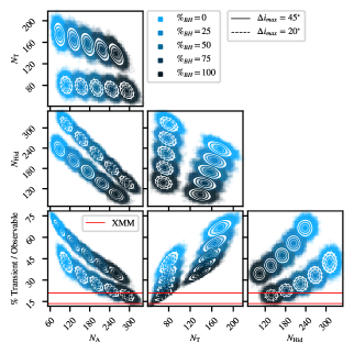
Figure 4: Shown are 2D 1$\sigma$ error contours for the distributions of the number of alive, transient and hidden systems ($N_{\rm A}$, $N_{\rm T}$, $N_{\rm Hid}$), as well as the percentage of transient to observed systems, ($N_{\rm T}/(N_{\rm A}+N_{\rm T}))$ and how these vary with the black hole percentage ($\%_{\mathrm{BH}}$) of the underlying population. This particular simulation used the following fixed parameters: $N_{\rm sys}=500$, $Z=0.02$, $\Delta i_{\mathrm{max}}=20^{\circ}$ (dashed contours) $45^{\circ}$ (solid contours) and $d=0.2$. $\%_{\mathrm{BH}}$ was varied between 0, 25, 50, 75 & 100%, where a higher abundance of BH systems is shown on the figure as darker colours and blue-er colours correspond to higher abundances of NS systems. The red lines denote the $1\sigma$ confidence bounds for the percentage of transient systems to observable systems obtained from the most recent XMM-Newton ULX catalogue (Earnshaw et al., 2019)

Having established in section 3.2 that the relative abundance of alive, hidden and transient sources may serve to provide diagnostic information on the quantities describing the underlying population, we now explore the broad implications for constraining the underlying nature of the observed ULX population using eROSITA.

Following the method described in section 2.8.1, we subject the transient light curves to regular sampling, matching the cadence of eRASS, and investigate whether any of our measured quantities, such as the relative number of transient to observed sources, are affected by our input parameters, e.g. the black hole percentage, maximum precessional angle or period prescription). Figure 6 shows three directly observable quantities and their evolution over the course of eRASS: the cumulative number of alive and transient ULXs, and the proportion of transient to total observed ULXs, for five different black hole ratios (with 1$\sigma$ bounds on the quantities via 10,000 MC iterations). The model parameters used to make Figure 6 are $Z=0.02$, $d=0.2$, $\Delta i_{\mathrm{max}}=45^{\circ}$ (left-hand column) & $20^{\circ}$ (right-hand column), and here we use the Lense-Thirring precession period (eqn 4).

3.3.2 Observational predictions for eRASS

From the first row of Figure 6, we observe the absolute number of alive sources detected by eRASS appears to be sensitive to the underlying black hole ratio, with the number being positively correlated with the proportion of BHs in the underlying populations. We also observe that the number of transient sources (middle row) detected by eRASS is not sensitive to the black hole ratio, i.e. for a given set of parameters ($Z$, $\Delta i_{\mathrm{max}}$, $d$ & $P$), the inferred 1$\sigma$ regions overlap. Instead we find that the number of transient sources is sensitive to the maximum precessional angle, with $\Delta i_{\mathrm{max}}=20^{\circ}$ providing around half the number of transients when compared to $\Delta i_{\mathrm{max}}=45^{\circ}$. This may mean that if we have a well-informed prior on the maximum precessional angle, we may, by considering the relative percentage of transient to observed sources obtain some indication of the black hole percentage in the underlying population.

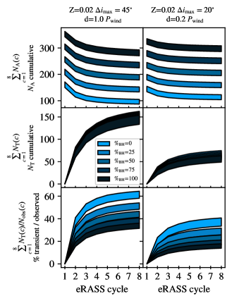
Figure 6: The evolution over eRASS cycles of three quantities that may be directly observed: the number of alive (top row), transient (middle) and proportion of transient to observed sources (bottom). Each column shows a different set of model parameters, while the different colours correspond to the underlying black hole ratio, with darker colours corresponding to a higher abundance of BHs. The width of the lines indicate the 1$\sigma$ error regions of the quantities being explored.

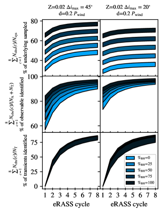
Figure 7: The evolution over eRASS cycles of the percentage of the underlying sources sampled (top), the percentage of the potentially observable sources sampled (middle) and percentage of transient sources sampled (bottom). The width of the lines indicate the 1$\sigma$ error regions of the quantities being explored.

In Figure 7 we also show three quantities not directly observable by eRASS but useful for gaining insight into the performance of the survey:

• $\sum_{c=1}^{8}N_{\rm obs}(c)/N_{\rm sys}$ provides the percentage of the full ULX population sampled by a given eRASS cycle

• $\sum_{c=1}^{8}N_{\rm obs}(c)/(N_{\rm A}+N_{\rm T})$ which quantifies the percentage of the potentially observable population which has been observed

• $\sum_{c=1}^{8}N_{\rm obs}(c)/N_{\rm T}$ which quantifies the percentage of the transient population only which was sampled

We will now briefly summarise the effect of each of our model parameters on the observed population as seen by eRASS.

• Effect of metallicity:

  Lower metallicity environments are commonly associated with a higher abundance of BH systems, as lower metallicity stars experience less mass loss than their higher metallicity counterparts and are therefore more likely to end up as BHs (Heger et al., 2003). However, as we are manually specifying the relative abundance of BHs in our simulations, the effect of $Z$ does not strongly correlate with many of our observable quantities.

• Effect of underlying demographic:

  Figure 6 shows the effect of changing the percentage of black holes within the sample, for a given set of model parameters over eRASS cycles. We observe that there is a sizeable increase in the number of alive systems for higher abundances of black holes. There is also an essentially constant number of transient sources across all black hole ratios. The combination of these last two effects means that the percentage of transient to observed sources also shows a dependence on the black hole ratio. For the set of simulation parameters shown in Figure 6, and for a maximum precessional angle of $45^{\circ}$, it can be seen that, for a population composed entirely of black holes, around $\sim 30\%$ of observed sources may be identified as transient by cycle eight, whilst up to $\sim 60\%$ would be observed as transient for a population composed entirely of neutron stars. For a maximum precessional angle of $20^{\circ}$, these values are instead around $\sim 20\%$ and $\sim 40\%$ respectively.

  From Figure 7 we also note that the underlying (both full and potentially observable) ULX populations are better sampled for higher black hole percentages in the underlying population.

• Effect of maximum precessional angle:

  While the Galactic ULX SS433 is well known to have a precessional half-angle of $\sim 20^{\circ}$ (Fabian & Rees, 1979), the light curve of NGC 5907 X-1 was described using ULXLC with a precessional half-angle of only $\Delta i=7.30^{+0.13}_{-0.15}$ (Dauser et al., 2017). With only two observational constraints (the one for NGC 5907 X-1 naturally being model-dependent), the precessional angle, $\Delta i$, remains one of the least constrained free parameters in our analysis. As such, we have throughout this work assumed a flat prior, however, the physics of the underlying precession mechanism (e.g. in the case of Lense-Thirring precession, the misalignment angle) could plausibly result in precessional angles which tend towards the smaller range of values.

  From Figure 6, a maximum precessional angle of $\Delta i_{\mathrm{max}}=45^{\circ}$ roughly halves the absolute number of transients detected in each eRASS cycle while also halving the percentage of transients to total observed systems when compared to a maximum precessional angle of $\Delta i_{\mathrm{max}}=20^{\circ}$. As seen in Figure 7, a larger precessional angle results in a higher number of the potentially observable (alive or dead) sources being identified but interestingly results in a lower proportion of the entire underlying population being sampled.

• Effect of the precession prescription:

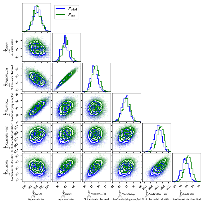
Figure 8: Corner plot comparing two precession mechanisms for cycle 3 of eRASS showing the minimal impact of using $P_{\mathrm{wind}}$ over $P_{\mathrm{sup}}$. Model parameters $Z=0.02$, $\%_{\mathrm{BH}}=50$, $\Delta i_{\mathrm{max}}$ $d=0.2$.

  Remarkably we find that both the empirical relation of Townsend & Charles (2020) (eq 7) and the prediction from the Lense-Thirring model (eq 4) produce similar results (see Figure 8). This is intriguing as it implies that, regardless of the mechanism, if the disc and wind are precessing then we can infer the properties of the underlying sample. Of course, should the mechanism be substantially different (e.g. precession of the curtain Mushtukov et al. 2017b), then this assertion may be invalid.

• Effect of the LMXB duty cycle:

  We find that a lower duty cycle for the LMXB ULX population serves to reduce the absolute number of transients detected in each cycle. However, when we consider the relative proportion of transients to the total number of observed sources, we find the impact of changing the duty cycle to be negligible.

4 Discussion

The relative proportion of black holes to neutron stars within the observed ULX population still remains an important unanswered question; of the current sample of roughly 500 ULXs, around ten are confirmed to have NS accretors, and there are strong indications that certain objects may harbour black holes (e.g. Cseh et al. 2014), but for the vast majority of the population, the nature of the accretor remains unknown. Wiktorowicz et al. (2019) approached this issue by analysing how anisotropic emission of radiation (geometrical beaming) affects the observed sample of ULXs, finding that, in regions of constant star formation, the expected number of NS ULXs is higher than the total number of BH ULXs, however due to the effect of beaming, they concluded that the total observed population was potentially comparable (cf. Middleton & King 2017). Our work has built on this by exploring the additional effect of precession of the wind cone.

Our simulations have allowed us to construct synthetic XLFs (Figure 2) and explore the changes resulting from varying the underlying population demographic. Fitting to only the high luminosity end (L $\geq 1\times 10^{39}\ \mathrm{erg}\ \mathrm{s}^{-1}$) appears to indicate a range of slopes which are somewhat steeper than observation (Table 2 and Figure 3) at least where the percentage of black holes in the underlying population are non-zero. It may be that the proportion of black holes is indeed low (as one would expect many more neutron stars than black holes in the intrinsic, underlying population: Wiktorowicz et al. 2019), however there are also several effects which may contribute to differences between simulation and observation. It is important to note that the XLFs we have created from simulation represent a time-averaged and idealised view of a large population of ULXs, whilst XLFs constructed from single (or from a small number of) observations instead suffer from a bias towards detecting bright, persistent ULXs rather than transient ULXs (and will also depend on the star formation history of the target galaxy which we have not accounted for Fragos et al. 2013a; Fragos et al. 2013b). We also note that – unlike the observational XLFs – our simulated luminosities do not assume any absorption; whilst accounting for this effect is complicated (it for instance depends on the unknown spectral shape and local column of a given ULX at a given point in its precessional cycle, e.g. Middleton et al. 2015), this is unlikely to have a major effect as long as the line-of-sight column is low. Finally, we have assumed a form for the beaming which does not take into account the full complexity of the system, e.g. radial collimation profile, re-processing and outwards advection, all as functions of accretion rate. These complicating effects could potentially bring the highest sources down to lower luminosities, making the XLF steeper.

One of the key results to emerge from our analysis is the indication that a measure of the relative number of transient to observed ULXs can constrain the nature of the intrinsic population. Such a result is naturally important as it would allow for a more concrete understanding of the accreting binary population and related fields (i.e. studies relying on binary population synthesis, e.g. Fragos et al. 2013b). However, it is important to consider the limitations of our approach. We have made the explicit assumption that either Lense-Thirring torques ($P_{\mathrm{wind}}$) or a different unspecified process $(P_{\mathrm{sup}}$: Townsend & Charles 2020) are the dominant form of variability on the timescales we are investigating. Whilst Lense-Thirring torques are certainly unavoidable where the compact object is misaligned (expected in light of the time required to align the binary – see King & Nixon 2018), there are other torques which can dilute or dominate over this effect. These are discussed at length in Middleton et al. (2018) but perhaps most notably we might expect radiation pressure driven warps and precession (Pringle, 1996), or neutron star dipole precession (see Mushtukov et al. 2017b) to occur where the field is very strong (in the case of the former, the outer disc can be essentially unshielded for high dipole field NSs, unless the accretion rate is extreme). We also note that free-body precession may occur as a result of neutron star oblateness and misalignment of the rotation axis with the axis of symmetry of the star (Jones & Andersson, 2001). This latter effect has been explored as an alternative origin for the month timescale modulation seen in ULXs (Vasilopoulos et al., 2020).

In addition – and unlike our consideration of the impact of a LMXB duty cycle – we have not included the effect of propeller states which occur when neutron stars are close to spin equilibrium. In such cases, increasing the neutron star spin by a small amount leads to a period of relative quiescence where emission from the accretion column and accretion curtain is switched off due to the centrifugal barrier. If the accretion rate is high or dipole field strength low enough, then we still expect radiation to emerge from the disc between $r_{\rm sph}$ and the magnetospheric radius, $r_{\rm M}$, which could be substantial (the luminosity then going as $\ln(r_{\rm sph}/r_{\rm M}$). However, where the dipole field strength is high or accretion rate low, entering a propellor state could effectively switch off most of the emission, potentially dropping the source below the empirical ULX threshold.

Throughout this work we have made the assumption that NSs have a low spin of $a_{*}=0.01$ while black holes have a maximal spin of $a_{*}=0.998$. The former is based on the observation of $\sim$1 s periods in ULX pulsars to-date (see King & Lasota 2020 and references in introduction). Naturally, we cannot rule out higher spins for NS systems (as an example, the fastest known spin frequency of a NS at 716Hz Hessels et al. 2006 would correspond to a maximal spin of $a_{*}=0.2-0.3$ Miller & Miller 2015, which would reduce the Lense-Thirring precession timescale accordingly, but the lack of evidence for such spins in ULXs presently limits our ability to explore this. Black hole ULXs may also not be maximally spinning (implying a slower precession period if Lense-Thirring), however, once again we have limited information at this time.

It is interesting to note that around half of the known PULXs appear to be transient ULXs, with luminosities spanning over a factor of 100 (Song et al., 2020). A propeller state has already been reported in one NS ULX to-date (Fürst et al. 2016, although the spin evolution implies the drop in flux is instead driven by obscuration/precession: Fürst et al. 2021). Earnshaw et al. (2018) have searched for propeller state ULXs within the entire XMM-Newton 3XMM-DR4 serendipitous source catalogue, identifying five ULXs that demonstrated long term variability over an order of magnitude in brightness, while one source (M51 ULX-4) demonstrates an apparent bi-modal flux distribution that may be consistent with a source undergoing propeller (although this may also be due to sampling a precessional light curve (e.g. Dauser et al. 2017). They also note that there are potentially up to $\sim 200$ sources in the XMM-Newton catalogue which may simply lack a sufficient number of observations using XMM-Newton to reveal their transient nature. Subsequent simulations by the same authors suggest that eROSITA may be able to identify 96% of sources that are undergoing the propeller effect by cycle 8 of eRASS (for a duty cycle of 0.5). This means that if NS ULXs undergoing the propeller effect are present in a large number within the population, the true number of transient sources in this paper could be largely underestimated.

In practice this means that, without an indication of whether a given source’s variability is driven by precession or propeller, the regular observations taken within eRASS may lead us to somewhat overestimate the underlying number of transients driven by precession (although this relies on the sample being large and not many sources precessing on very long timescales). As a result, we would tend to over-estimate the abundance of neutron stars in the underlying population. However, if we are able to isolate sources that display precession (e.g. via fitting of long term light-curves or ruling out the propeller effect), then, given a large enough sample, we would then obtain a lower limit on the number of transient (via precession) to observed sources and a lower limit on the the abundance of neutron stars in the underlying population.

Finally, we have assumed that NSs in our simulations may only reach ULX luminosities via geometrical beaming, while it is possible that a drop in the electron scattering cross section due to a high strength magnetic field, as well as the structure of the accretion column itself could also boost the luminosity (e.g. Basko & Sunyaev 1976; Mushtukov et al. 2017b).

5 Conclusions

Starting from a synthetic population of binary systems, and using a simple geometrical model for a precessing cone of emission, we have investigated the effect precession and beaming might together play on the observed population of ULXs. We have investigated the effect precession has on the XLF and the relative numbers of alive (persistently $\geq$ 1$\times$10${}^{39}\ \mathrm{erg}\ \mathrm{s}^{-1}$), transient (varying across 1$\times$10${}^{39}\ \mathrm{erg}\ \mathrm{s}^{-1}$) and hidden (persistently $<$ 1$\times$10${}^{39}\ \mathrm{erg}\ \mathrm{s}^{-1}$) sources, and, by factoring in the observational cadence of eRASS, we have made predictions for how well the underlying population may be constrained over the course of four years of monitoring.

In this paper we propose a novel method for constraining the underlying demographic within the population of ULXs, as the percentage of ULXs observed to be transient or observed is sensitive to parameters such as maximum precessional angle, and crucially to the relative fraction of BHs and NSs in the underlying population (whilst not sensitive to the duty cycle of LMXB ULXs). This follows from the fact that – under the assumptions of geometrical beaming – populations containing a higher percentage of BHs are observationally associated with higher percentages of systems persistently above $10^{39}\ \mathrm{erg}\ \mathrm{s}^{-1}$ and with lower percentages of transient systems, when compared to populations dominated by NSs.

Determining the underlying ULX demographic presently relies on detecting unambiguous indicators for the presence of a neutron star such as pulsations or a CRSF. However, it has been proposed that many NS ULXs with high accretion rates may not exhibit pulsations King et al. (2017), that large pulse fractions may be absent in the presence of strong beaming (Mushtukov et al., 2021b), and CRSFs may not fall within the accessible X-ray energy range or may be diluted (see Mushtukov et al. 2017a). An independent and simple method to constrain the nature of the underlying population in ULXs such as the one we have explored here is therefore of value (and joins others such as observing the evolution of quasi-periodic oscillations, see Middleton et al. 2019b).

In an initial application of our approach, we have used the Earnshaw et al. (2019) catalogue of ULX and ULX candidates (accepting that this catalogue is incomplete relative to a true flux-limited survey). Finding that $\sim 80\%$ of the catalogue ULXs are always visible, while $\sim 20\%$ are transient; this implies a black hole percentage in the underlying population in the region of $10-100\%$ (for $\Delta i_{\rm max}\leq 20^{\circ}$) or $75-100\%$ (for $\Delta i_{\rm max}\leq 45^{\circ}$). However, the number of transients (which we expect to be mostly neutron star ULXs) is likely to be highly underestimated in such low cadence, pointed observing. The introduction of eROSITA and its all sky survey, eRASS, will revolutionise our view of the transient X-ray sky and is optimally placed to better constrain the underlying demographic of ULXs via this approach. Simulating using two different prescriptions for the precession period: Lense-Thirring (Middleton et al. 2019b) and empirical (Townsend & Charles 2020), we predict a variety of observational possibilities for the evolution of the relative numbers of transient to persistent ULXs over the course of eRASS, for a variety of population characteristics. We conclude that neither prescription for precession significantly alters our observed view of the ULX population.

We have invoked several simplifications in this work which we will improve upon in future. Our model for precession (ULXLC) currently does not account for the energy dependence of the emission; we are developing models which account for the radial dependence of beaming and which will improve on the accuracy of our simulations. We also presently have limited constraints on the precession angle of the wind cone in ULXs which can have a significant impact on our predictions; this can be estimated through direct modelling (Dauser et al., 2017) and, in future, will be developed and applied more widely to improve our constraints. Finally, we have not included the effects of magnetic fields in the neutron star systems in our population; this can have the effect of changing the X-ray spectrum and beaming but, perhaps more importantly, can lead to periods of relative quiescence via the propeller effect (Fürst et al., 2016; Earnshaw et al., 2018) as well as dipole precession on $\sim$month timescales when the field is very strong (Lipunov & Shakura, 1980).

Data Availability

The data obtained from StarTrack underlying this article are freely accessible at the following urls:
https://universeathome.pl/universe/pub/z02_data1.dat
https://universeathome.pl/universe/pub/z002_data1.dat
https://universeathome.pl/universe/pub/z0002_data1.dat

Appendix A Comparison of Period Prescriptions

References

- Bachetti et al. (2014) Bachetti M., et al., 2014, Nature, 514, 202
- Basko & Sunyaev (1976) Basko M. M., Sunyaev R. A., 1976, MNRAS, 175, 395
- Belczynski et al. (2008) Belczynski K., Kalogera V., Rasio F. A., Taam R. E., Zezas A., Bulik T., Maccarone T. J., Ivanova N., 2008, The Astrophysical Journal Supplement Series, 174, 223
- Belczynski et al. (2020) Belczynski K., et al., 2020, A&A, 636, A104
- Brightman et al. (2018) Brightman M., et al., 2018, Nature Astronomy, 2, 312
- Burke et al. (2013) Burke M. J., et al., 2013, ApJ, 775, 21
- Cappelluti et al. (2011) Cappelluti N., et al., 2011, Memorie della Societa Astronomica Italiana Supplementi, 17, 159
- Carpano et al. (2018) Carpano S., Haberl F., Maitra C., Vasilopoulos G., 2018, MNRAS, 476, L45
- Clauset et al. (2007) Clauset A., Rohilla Shalizi C., Newman M. E. J., 2007, arXiv e-prints, p. arXiv:0706.1062
- Colbert & Mushotzky (1999) Colbert E. J. M., Mushotzky R. F., 1999, ApJ, 519, 89
- Cseh et al. (2014) Cseh D., et al., 2014, MNRAS, 439, L1
- Dauser et al. (2017) Dauser T., Middleton M., Wilms J., 2017, MNRAS, 466, 2236
- Deegan et al. (2009) Deegan P., Combet C., Wynn G. A., 2009, MNRAS, 400, 1337
- Doroshenko et al. (2018) Doroshenko V., Tsygankov S., Santangelo A., 2018, A&A, 613, A19
- Earnshaw et al. (2018) Earnshaw H. P., Roberts T. P., Sathyaprakash R., 2018, MNRAS, 476, 4272
- Earnshaw et al. (2019) Earnshaw H. P., Roberts T. P., Middleton M. J., Walton D. J., Mateos S., 2019, MNRAS, 483, 5554
- Everitt et al. (2011) Everitt C. W. F., et al., 2011, Physical Review Letters, 106, 221101
- Fabbiano (1989) Fabbiano G., 1989, ARA&A, 27, 87
- Fabian & Rees (1979) Fabian A. C., Rees M. J., 1979, MNRAS, 187, 13P
- Fabrika (2004) Fabrika S., 2004, APSPR, 12, 1
- Feng & Kaaret (2007) Feng H., Kaaret P., 2007, ApJ, 660, L113
- Foreman-Mackey et al. (2021) Foreman-Mackey D., et al., 2021, dfm/corner.py: corner.py v.2.2.1, doi:10.5281/zenodo.4592454, https://doi.org/10.5281/zenodo.4592454
- Fragile et al. (2007) Fragile P. C., Blaes O. M., Anninos P., Salmonson J. D., 2007, ApJ, 668, 417
- Fragos et al. (2013a) Fragos T., et al., 2013a, ApJ, 764, 41
- Fragos et al. (2013b) Fragos T., Lehmer B. D., Naoz S., Zezas A., Basu-Zych A., 2013b, ApJ, 776, L31
- Fürst et al. (2016) Fürst F., et al., 2016, ApJ, 831, L14
- Fürst et al. (2021) Fürst F., et al., 2021, A&A, 651, A75
- Grimm et al. (2003) Grimm H. J., Gilfanov M., Sunyaev R., 2003, MNRAS, 339, 793
- Hameury & Lasota (2020) Hameury J.-M., Lasota J.-P., 2020, arXiv e-prints, p. arXiv:2010.00365
- Heger et al. (2003) Heger A., Fryer C. L., Woosley S. E., Langer N., Hartmann D. H., 2003, ApJ, 591, 288
- Hessels et al. (2006) Hessels J. W. T., Ransom S. M., Stairs I. H., Freire P. C. C., Kaspi V. M., Camilo F., 2006, Science, 311, 1901
- Ingram & Done (2012a) Ingram A., Done C., 2012a, MNRAS, 419, 2369
- Ingram & Done (2012b) Ingram A., Done C., 2012b, MNRAS, 427, 934
- Ingram et al. (2017) Ingram A., van der Klis M., Middleton M., Altamirano D., Uttley P., 2017, MNRAS, 464, 2979
- Israel et al. (2017) Israel G. L., et al., 2017, Science, 355, 817
- Jiang et al. (2014) Jiang Y.-F., Stone J. M., Davis S. W., 2014, ApJ, 796, 106
- Jiang et al. (2019) Jiang Y.-F., Stone J. M., Davis S. W., 2019, ApJ, 880, 67
- Jones & Andersson (2001) Jones D. I., Andersson N., 2001, MNRAS, 324, 811
- Kaaret et al. (2006) Kaaret P., Simet M. G., Lang C. C., 2006, Science, 311, 491
- Kaaret et al. (2017) Kaaret P., Feng H., Roberts T. P., 2017, ARA&A, 55, 303
- Kajava & Poutanen (2009) Kajava J. J. E., Poutanen J., 2009, MNRAS, 398, 1450
- King (2009) King A. R., 2009, Monthly Notices of the Royal Astronomical Society, 393, L41
- King & Lasota (2019) King A., Lasota J.-P., 2019, MNRAS, 485, 3588
- King & Lasota (2020) King A., Lasota J.-P., 2020, MNRAS,
- King & Nixon (2018) King A., Nixon C., 2018, ApJ, 857, L7
- King & Puchnarewicz (2002) King A. R., Puchnarewicz E. M., 2002, MNRAS, 336, 445
- King et al. (2001) King A. R., Davies M. B., Ward M. J., Fabbiano G., Elvis M., 2001, ApJ, 552, L109
- King et al. (2017) King A., Lasota J.-P., Kluźniak W., 2017, MNRAS, 468, L59
- Koliopanos et al. (2019) Koliopanos F., Vasilopoulos G., Buchner J., Maitra C., Haberl F., 2019, A&A, 621, A118
- Kong et al. (2016) Kong A. K. H., Hu C.-P., Lin L. C.-C., Li K. L., Jin R., Liu C. Y., Yen D. C.-C., 2016, MNRAS, 461, 4395
- Kosec et al. (2018a) Kosec P., Pinto C., Fabian A. C., Walton D. J., 2018a, MNRAS, 473, 5680
- Kosec et al. (2018b) Kosec P., Pinto C., Walton D. J., Fabian A. C., Bachetti M., Brightman M., Fürst F., Grefenstette B. W., 2018b, MNRAS, 479, 3978
- Kovlakas et al. (2020) Kovlakas K., Zezas A., Andrews J. J., Basu-Zych A., Fragos T., Hornschemeier A., Lehmer B., Ptak A., 2020, MNRAS, 498, 4790
- Lasota (2001) Lasota J.-P., 2001, New Astron. Rev., 45, 449
- Lasota et al. (2016) Lasota J. P., Vieira R. S. S., Sadowski A., Narayan R., Abramowicz M. A., 2016, A&A, 587, A13
- Lei et al. (2013) Lei W.-H., Zhang B., Gao H., 2013, ApJ, 762, 98
- Lipunov & Shakura (1980) Lipunov V. M., Shakura N. I., 1980, Soviet Astronomy Letters, 6, 14
- Maccarone et al. (2007) Maccarone T. J., Kundu A., Zepf S. E., Rhode K. L., 2007, Nature, 445, 183
- Maloney & Begelman (1997) Maloney P. R., Begelman M. C., 1997, ApJ, 491, L43
- Maloney et al. (1998) Maloney P. R., Begelman M. C., Nowak M. A., 1998, ApJ, 504, 77
- Margon et al. (1979) Margon B., Grandi S. A., Downes R., 1979, in Bulletin of the American Astronomical Society. p. 786
- Merloni et al. (2012) Merloni A., et al., 2012, arXiv e-prints, p. arXiv:1209.3114
- Middleton & King (2017) Middleton M. J., King A., 2017, MNRAS, 470, L69
- Middleton et al. (2014) Middleton M. J., Walton D. J., Roberts T. P., Heil L., 2014, MNRAS, 438, L51
- Middleton et al. (2015) Middleton M. J., Walton D. J., Fabian A., Roberts T. P., Heil L., Pinto C., Anderson G., Sutton A., 2015, MNRAS, 454, 3134
- Middleton et al. (2018) Middleton M. J., et al., 2018, MNRAS, 475, 154
- Middleton et al. (2019a) Middleton M. J., Brightman M., Pintore F., Bachetti M., Fabian A. C., Fürst F., Walton D. J., 2019a, MNRAS, 486, 2
- Middleton et al. (2019b) Middleton M. J., Fragile P. C., Ingram A., Roberts T. P., 2019b, MNRAS, 489, 282
- Middleton et al. (2021) Middleton M. J., et al., 2021, MNRAS,
- Milgrom (1979) Milgrom M., 1979, A&A, 78, L9
- Miller & Miller (2015) Miller M. C., Miller J. M., 2015, Phys. Rep., 548, 1
- Mineo et al. (2012) Mineo S., Gilfanov M., Sunyaev R., 2012, MNRAS, 419, 2095
- Motta et al. (2018) Motta S. E., Franchini A., Lodato G., Mastroserio G., 2018, Monthly Notices of the Royal Astronomical Society, 473, 431
- Mushtukov (2018) Mushtukov A., 2018, in 42nd COSPAR Scientific Assembly. pp E1.13–1–18
- Mushtukov et al. (2017a) Mushtukov A., Suleimanov V., Tsygankov S., Poutanen J., 2017a, in Ness J.-U., Migliari S., eds, The X-ray Universe 2017. p. 153
- Mushtukov et al. (2017b) Mushtukov A. A., Suleimanov V. F., Tsygankov S. S., Ingram A., 2017b, MNRAS, 467, 1202
- Mushtukov et al. (2021a) Mushtukov A. A., Portegies Zwart S., Tsygankov S. S., Nagirner D. I., Poutanen J., 2021a, MNRAS, 501, 2424
- Mushtukov et al. (2021b) Mushtukov A. A., Portegies Zwart S., Tsygankov S. S., Nagirner D. I., Poutanen J., 2021b, MNRAS, 501, 2424
- Pasham & Strohmayer (2013) Pasham D. R., Strohmayer T. E., 2013, ApJ, 774, L16
- Pinto et al. (2016) Pinto C., Middleton M. J., Fabian A. C., 2016, Nature, 533, 64
- Pinto et al. (2017) Pinto C., Fabian A., Middleton M., Walton D., 2017, Astronomische Nachrichten, 338, 234
- Poutanen et al. (2007) Poutanen J., Lipunova G., Fabrika S., Butkevich A. G., Abolmasov P., 2007, MNRAS, 377, 1187
- Predehl et al. (2020) Predehl P., et al., 2020, arXiv e-prints, p. arXiv:2010.03477
- Predehl et al. (2021) Predehl P., et al., 2021, A&A, 647, A1
- Pringle (1996) Pringle J. E., 1996, MNRAS, 281, 357
- Reig (2011) Reig P., 2011, Ap&SS, 332, 1
- Roberts (2007) Roberts T. P., 2007, Ap&SS, 311, 203
- Rodríguez Castillo et al. (2020) Rodríguez Castillo G. A., et al., 2020, ApJ, 895, 60
- Rosen et al. (2016) Rosen S. R., et al., 2016, A&A, 590, A1
- Rubin et al. (1998) Rubin B. C., Harmon B. A., Paciesas W. S., Robinson C. R., Zhang S. N., Fishman G. J., 1998, ApJ, 492, L67
- Sathyaprakash et al. (2019) Sathyaprakash R., et al., 2019, MNRAS, 488, L35
- Shakura & Sunyaev (1973) Shakura N. I., Sunyaev R. A., 1973, A&A, 500, 33
- Sądowski et al. (2014) Sądowski A., Narayan R., McKinney J. C., Tchekhovskoy A., 2014, MNRAS, 439, 503
- Song et al. (2020) Song X., Walton D. J., Lansbury G. B., Evans P. A., Fabian A. C., Earnshaw H., Roberts T. P., 2020, MNRAS, 491, 1260
- Steele et al. (2014) Steele M. M., Zepf S. E., Maccarone T. J., Kundu A., Rhode K. L., Salzer J. J., 2014, ApJ, 785, 147
- Stella & Vietri (1998) Stella L., Vietri M., 1998, ApJ, 492, L59
- Swartz et al. (2011) Swartz D. A., Soria R., Tennant A. F., Yukita M., 2011, ApJ, 741, 49
- Townsend & Charles (2020) Townsend L. J., Charles P. A., 2020, MNRAS, 495, 139
- Tsygankov et al. (2017) Tsygankov S. S., Doroshenko V., Lutovinov A. A., Mushtukov A. A., Poutanen J., 2017, A&A, 605, A39
- Vasilopoulos et al. (2019) Vasilopoulos G., Petropoulou M., Koliopanos F., Ray P. S., Bailyn C. B., Haberl F., Gendreau K., 2019, MNRAS, 488, 5225
- Vasilopoulos et al. (2020) Vasilopoulos G., Lander S. K., Koliopanos F., Bailyn C. D., 2020, MNRAS, 491, 4949
- Walton et al. (2016a) Walton D. J., et al., 2016a, ApJ, 826, L26
- Walton et al. (2016b) Walton D. J., et al., 2016b, ApJ, 827, L13
- Walton et al. (2018) Walton D. J., et al., 2018, ApJ, 857, L3
- Wang et al. (2016) Wang S., Qiu Y., Liu J., Bregman J. N., 2016, ApJ, 829, 20
- Wiktorowicz et al. (2017) Wiktorowicz G., Sobolewska M., Lasota J.-P., Belczynski K., 2017, ApJ, 846, 17
- Wiktorowicz et al. (2019) Wiktorowicz G., Lasota J.-P., Middleton M., Belczynski K., 2019, ApJ, 875, 53
- Wolter et al. (2018) Wolter A., Fruscione A., Mapelli M., 2018, ApJ, 863, 43