CLOOB: Modern Hopfield Networks with
InfoLOOB Outperform CLIP

Abstract

CLIP yielded impressive results on zero-shot transfer learning tasks and is considered as a foundation model like BERT or GPT3. CLIP vision models that have a rich representation are pre-trained using the InfoNCE objective and natural language supervision before they are fine-tuned on particular tasks. Though CLIP excels at zero-shot transfer learning, it suffers from an explaining away problem, that is, it focuses on one or few features, while neglecting other relevant features. This problem is caused by insufficiently extracting the covariance structure in the original multi-modal data. We suggest to use modern Hopfield networks to tackle the problem of explaining away. Their retrieved embeddings have an enriched covariance structure derived from co-occurrences of features in the stored embeddings. However, modern Hopfield networks increase the saturation effect of the InfoNCE objective which hampers learning. We propose to use the InfoLOOB objective to mitigate this saturation effect. We introduce the novel “Contrastive Leave One Out Boost” (CLOOB), which uses modern Hopfield networks for covariance enrichment together with the InfoLOOB objective. In experiments we compare CLOOB to CLIP after pre-training on the Conceptual Captions and the YFCC dataset with respect to their zero-shot transfer learning performance on other datasets. CLOOB consistently outperforms CLIP at zero-shot transfer learning across all considered architectures and datasets.

1 Introduction

Contrastive Language-Image Pre-training (CLIP) showed spectacular performance at zero-shot transfer learning (Radford et al., 2021). CLIP learns expressive image embeddings directly from raw text, thereby leverages a much richer source of supervision than just labels. The CLIP model is considered as an important foundation model (Bommasani et al., 2021), therefore a plethora of follow-up work has been published (see Appendix Section A.4). CLIP as a contrastive learning method has two simultaneous goals, namely (i) increasing the similarity of matched language-image pairs and (ii) decreasing the similarity of unmatched language-image pairs. Though CLIP yielded striking zero-shot transfer learning results, it still suffers from “explaining away”. Explaining away is known in reasoning as the concept that the confirmation of one cause of an observed event dismisses alternative causes (Pearl, 1988; Wellman & Henrion, 1993). CLIP’s explaining away problem is its focus on one or few features while neglecting other relevant features. This problem is caused by insufficiently extracting feature co-occurrences and covariance structures in the original multi-modal data. Humans extract co-occurrences and covariances by associating current perceptions with memories (Bonner & Epstein, 2021; Potter, 2012). In analogy to these human cognitive processes, we suggest to use modern Hopfield networks to amplify co-occurrences and covariance structures of the original data.

Hopfield networks are energy-based, binary associative memories, which popularized artificial neural networks in the 1980s (Amari, 1972; Hopfield, 1982, 1984). Associative memory networks have been designed to store and retrieve samples. Their storage capacity can be considerably increased by polynomial terms in the energy function (Chen et al., 1986; Psaltis & Cheol, 1986; Baldi & Venkatesh, 1987; Gardner, 1987; Abbott & Arian, 1987; Horn & Usher, 1988; Caputo & Niemann, 2002; Krotov & Hopfield, 2016). In contrast to these binary memory networks, we use continuous associative memory networks with very high storage capacity. These modern Hopfield networks for deep learning architectures have an energy function with continuous states and can retrieve samples with only one update (Ramsauer et al., 2021). Modern Hopfield networks have already been successfully applied to immune repertoire classification (Widrich et al., 2020), chemical reaction prediction (Seidl et al., 2022) and reinforcement learning (Widrich et al., 2021; Paischer et al., 2022). Modern Hopfield networks are a novel concept for contrastive learning to extract more covariance structure.

However, modern Hopfield networks lead to a higher similarity of retrieved samples. The increased similarity exacerbates the saturation of CLIP’s InfoNCE objective (van den Oord et al., 2018). InfoNCE saturates because it contains terms of the form $a/(a+b)$. In analogy to Wang & Isola (2020), $a$ is called the “alignment score” that measures the similarity of matched pairs and $b$ is called the “uniformity penalty” that measures the similarity of unmatched pairs. The saturation problem becomes more severe for retrieved samples of the modern Hopfield network since the alignment score $a$ increases. Saturation of InfoNCE hampers the decrease of the uniformity penalty $b$ (see also Yeh et al. (2021)). Contrary to InfoNCE, the “InfoLOOB” (LOOB for “Leave One Out Bound”) objective (Poole et al., 2019) contains only terms of the form $a/b$ which do not saturate. Thus, even for a large alignment score $a$, learning still decreases the uniformity penalty $b$ by distributing samples more uniformly.

We introduce “Contrastive Leave One Out Boost” (CLOOB) which combines modern Hopfield networks with the “InfoLOOB” objective. Our contributions are:

(a)

we propose CLOOB, a new contrastive learning method,

(b)

we propose modern Hopfield networks to reinforce covariance structures,

(c)

we propose InfoLOOB as an objective to avoid saturation as observed with InfoNCE, and provide theoretical justifications for optimizing InfoLOOB.

2 CLOOB: Modern Hopfield Networks with InfoLOOB

Our novel contrastive learning method CLOOB can be seen as a replacement of CLIP and therefore be used in any method which builds upon CLIP. Figure 1 sketches the CLOOB architecture for image-text pairs. The training set consists of $N$ pairs of embeddings $\{(\bm{x}_{1},\bm{y}_{1}),\ldots,(\bm{x}_{N},\bm{y}_{N})\}$ with $\bm{X}=(\bm{x}_{1},\ldots,\bm{x}_{N})$ and $\bm{Y}=(\bm{y}_{1},\ldots,\bm{y}_{N})$, $M$ stored embeddings $\bm{U}=(\bm{u}_{1},\ldots,\bm{u}_{M})$, and $K$ stored embeddings $\bm{V}=(\bm{v}_{1},\ldots,\bm{v}_{K})$. The state or query embeddings $\bm{x}_{i}$ and $\bm{y}_{i}$ retrieve $\bm{U}_{\bm{x}_{i}}$ and $\bm{U}_{\bm{y}_{i}}$, respectively, from $\bm{U}$ — analog for retrievals from $\bm{V}$. The samples are normalized: ${{\left\|\bm{x}_{i}\right\|}}={{\left\|\bm{y}_{i}\right\|}}={{\left\|\bm{u}_{i}\right\|}}={{\left\|\bm{v}_{i}\right\|}}=1$. $\bm{U}_{\bm{x}_{i}}$ denotes an image-retrieved image embedding, $\bm{U}_{\bm{y}_{i}}$ a text-retrieved image embedding, $\bm{V}_{\bm{x}_{i}}$ an image-retrieved text embedding and $\bm{V}_{\bm{y}_{i}}$ a text-retrieved text embedding. These retrievals from modern Hopfield networks are computed as follows (Ramsauer et al., 2021):

$$\bm{U}_{\bm{x}_{i}}\ =\ \bm{U}\ \mathrm{softmax}(\beta\ \bm{U}^{T}\bm{x}_{i})\ ,$$ (1)

$$\bm{U}_{\bm{y}_{i}}\ =\ \bm{U}\ \mathrm{softmax}(\beta\ \bm{U}^{T}\bm{y}_{i})\ ,$$ (2)

$$\bm{V}_{\bm{x}_{i}}\ =\ \bm{V}\ \mathrm{softmax}(\beta\ \bm{V}^{T}\bm{x}_{i})\ ,$$ (3)

$$\bm{V}_{\bm{y}_{i}}\ =\ \bm{V}\ \mathrm{softmax}(\beta\ \bm{V}^{T}\bm{y}_{i})\ .$$ (4)

\begin{overpic}[scale={0.85},percent]{figures/paper/CLOOB_sketch.pdf} \scriptsize \put(26.5,36.35){$\bm{x}_{1}$} \put(31.3,36.35){$\bm{x}_{2}$} \put(35.5,36.35){$\cdots$} \put(40.6,36.35){$\bm{x}_{N}$} \put(25.1,28.6){$\bm{U}_{\bm{x}_{1}}$} \put(29.9,28.6){$\bm{U}_{\bm{x}_{2}}$} \put(35.5,28.6){$\cdots$} \put(39.2,28.6){$\bm{U}_{\bm{x}_{N}}$} \par\put(51.2,36.35){$\bm{x}_{1}$} \put(56.0,36.35){$\bm{x}_{2}$} \put(60.2,36.35){$\cdots$} \put(65.3,36.35){$\bm{x}_{N}$} \put(50.0,28.6){$\bm{V}_{\bm{x}_{1}}$} \put(54.7,28.6){$\bm{V}_{\bm{x}_{2}}$} \put(60.2,28.6){$\cdots$} \put(64.1,28.6){$\bm{V}_{\bm{x}_{N}}$} \par\put(26.5,7.5){$\bm{y}_{1}$} \put(31.3,7.5){$\bm{y}_{2}$} \put(35.5,7.5){$\cdots$} \put(40.6,7.5){$\bm{y}_{N}$} \put(25.1,15.2){$\bm{U}_{\bm{y}_{1}}$} \put(29.9,15.2){$\bm{U}_{\bm{y}_{2}}$} \put(35.5,15.2){$\cdots$} \put(39.2,15.2){$\bm{U}_{\bm{y}_{N}}$} \par\put(51.2,7.5){$\bm{y}_{1}$} \put(56.0,7.5){$\bm{y}_{2}$} \put(60.2,7.5){$\cdots$} \put(65.3,7.5){$\bm{y}_{N}$} \put(50.0,15.2){$\bm{V}_{\bm{y}_{1}}$} \put(54.7,15.2){$\bm{V}_{\bm{y}_{2}}$} \put(60.2,15.2){$\cdots$} \put(64.1,15.2){$\bm{V}_{\bm{y}_{N}}$} \par\put(26.6,32.3){{Hopfield retrieval with} $\bm{U}$} \put(51.4,32.3){{Hopfield retrieval with} $\bm{V}$} \par\put(26.6,11.3){{Hopfield retrieval with} $\bm{U}$} \put(51.4,11.3){{Hopfield retrieval with} $\bm{V}$} \par\put(27.91,24.7){$\boldsymbol{\simeq}$} \put(32.9,24.7){$\boldsymbol{\simeq}$} \put(42.77,24.7){$\boldsymbol{\simeq}$} \par\put(52.65,19.2){$\boldsymbol{\simeq}$} \put(57.65,19.2){$\boldsymbol{\simeq}$} \put(67.5,19.2){$\boldsymbol{\simeq}$} \par\put(17.5,40.25){{image}} \put(17.5,38.25){{encoder}} \par\put(17.5,5.65){{text}} \put(17.5,3.65){{encoder}} \par\put(1.2,7.1){{Our dog is}} \put(1.2,5.1){{playing in}} \put(1.2,3.1){{the snow.}} \par\put(79.2,24.3){$\boldsymbol{\simeq}$} \put(85.0,28.0){{{legend}}} \put(83.0,24.2){{similarity to anchor}} \put(83.0,20.6){{positive sample}} \put(83.0,17.0){{negative sample}} \end{overpic}

Figure 1: The CLOOB architecture for image-text pairs. The image embedding $\bm{x}_{i}$ and the text embedding $\bm{y}_{i}$ retrieve the embeddings $\bm{U}_{\bm{x}_{i}}$ and $\bm{U}_{\bm{y}_{i}}$, respectively, from a modern Hopfield network that stores image embeddings $\bm{U}=(\bm{u}_{1},\ldots,\bm{u}_{M})$ (green boxes at the left). The image-retrieved image embedding $\bm{U}_{\bm{x}_{i}}$ serves as anchor in order to contrast the positive text-retrieved image embedding $\bm{U}_{\bm{y}_{i}}$ with the negative text-retrieved image embedding $\bm{U}_{\bm{y}_{j}}$ for $j\neq i$. Analogously, for the second modern Hopfield network that stores text embeddings $\bm{V}=(\bm{v}_{1},\ldots,\bm{v}_{K})$ (green boxes at the right).

The hyperparameter $\beta$ corresponds to the inverse temperature: $\beta=0$ retrieves the average of the stored pattern, while large $\beta$ retrieves the stored pattern that is most similar to the state pattern (query).

In the InfoLOOB loss Eq. (8), CLOOB substitutes the embedded samples $\bm{x}_{i}$ and $\bm{y}_{i}$ by the normalized retrieved embedded samples. In the first term, $\bm{x}_{i}$ and $\bm{y}_{i}$ are substituted by $\bm{U}_{\bm{x}_{i}}$ and $\bm{U}_{\bm{y}_{i}}$, respectively, while in the second term they are substituted by $\bm{V}_{\bm{x}_{i}}$ and $\bm{V}_{\bm{y}_{i}}$. After retrieval, the samples are re-normalized to ensure ${{\left\|\bm{U}_{\bm{x}_{i}}\right\|}}={{\left\|\bm{U}_{\bm{y}_{i}}\right\|}}={{\left\|\bm{V}_{\bm{x}_{i}}\right\|}}={{\left\|\bm{V}_{\bm{y}_{i}}\right\|}}=1$.

We obtain the CLOOB loss function:

$$\mathrm{L}_{\mathrm{InfoLOOB}}\ =\ -\ \frac{1}{N}\ \sum_{i=1}^{N}\ \ln\frac{\exp(\tau^{-1}\ \bm{U}_{\bm{x}_{i}}^{T}\bm{U}_{\bm{y}_{i}})}{\sum_{j\neq i}^{N}\exp(\tau^{-1}\ \bm{U}_{\bm{x}_{i}}^{T}\bm{U}_{\bm{y}_{j}})}\ -\ \frac{1}{N}\ \sum_{i=1}^{N}\ \ln\frac{\exp(\tau^{-1}\ \bm{V}_{\bm{x}_{i}}^{T}\bm{V}_{\bm{y}_{i}})}{\sum_{j\neq i}^{N}\exp(\tau^{-1}\ \bm{V}_{\bm{x}_{j}}^{T}\bm{V}_{\bm{y}_{i}})}\ .$$ (5)

By default, we store the minibatch in the modern Hopfield networks, that is, $\bm{U}=\bm{X}$ and $\bm{V}=\bm{Y}$. Thus, in Eq. (1) $\bm{x}_{i}$ can retrieve itself from $\bm{U}=\bm{X}$, but in Eq. (3) it can not retrieve itself from $\bm{V}=\bm{Y}$. Analogously, in Eq. (4) $\bm{y}_{i}$ can retrieve itself from $\bm{V}=\bm{Y}$, but in Eq. (2) it can not retrieve itself from $\bm{U}=\bm{X}$. By storing the embeddings of the mini-batch examples in the Hopfield memory, we do not require to compute the embeddings of additional samples via text and image encoders. However, the modern Hopfield networks can also store prototypes, templates, or proprietary samples to amplify particular embedding features via the stored samples. Either the original embeddings $\bm{x}$ and $\bm{y}$ or the retrieved embeddings $\bm{U}_{\bm{x}}$, $\bm{U}_{\bm{y}}$, $\bm{V}_{\bm{x}}$, and $\bm{V}_{\bm{y}}$ may serve for the downstream tasks, e.g. for zero-shot transfer learning.

Pseudocode 1 shows CLOOB in a PyTorch-like style. CLOOB has two major components: (i) modern Hopfield networks that alleviate CLIP’s problem of insufficiently exploiting the covariance structure in the data and (ii) the InfoLOOB objective that does not suffer from InfoNCE’s saturation problem. The next two sections analyze CLOOB’s major components.

Pseudocode 1 CLOOB in a PyTorch-like style.

⬇

1# image_encoder - ResNet

2# text_encoder - Text Transformer

3# I[n, h, w, c] - minibatch of images

4# T[n, l] - minibatch of texts

5# W_i[d_i, d_e] - image projection

6# W_t[d_t, d_e] - text projection

7# beta - inverse temperature Hopfield retrieval

8# tau - temperature InfoLOOB

9

10# extract feature representations

11I_f = image_encoder(I) #[n, d_i]

12T_f = text_encoder(T) #[n, d_t]

13

14# joint multimodal embedding

15x = l2_normalize(I_f @ W_i) #[n, d_e]

16y = l2_normalize(T_f @ W_t) #[n, d_e]

17

18# Hopfield retrieval H with batch stored

19# H(beta, A, B) = B.T @ softmax(beta * A @ B.T)

20U_x = H(beta, x, x).T #[n, d_e]

21U_y = H(beta, y, x).T #[n, d_e]

22V_x = H(beta, x, y).T #[n, d_e]

23V_y = H(beta, y, y).T #[n, d_e]

24

25# normalize retrievals

26U_x = l2_normalize(U_x) #[n, d_e]

27U_y = l2_normalize(U_y) #[n, d_e]

28V_x = l2_normalize(V_x) #[n, d_e]

29V_y = l2_normalize(V_y) #[n, d_e]

30

31# loss: info_loob(tau, anchors, samples)

32# samples contain pos. and neg. embeddings

33loss_i = info_loob(tau, U_x, U_y)

34loss_t = info_loob(tau, V_y, V_x)

35loss = (loss_i + loss_t) * tau

3 Modern Hopfield Networks for Enriching the Covariance Structure

We use modern Hopfield networks to amplify co-occurrences and the covariance structure. Replacing the original embeddings by retrieved embeddings reinforces features that frequently occur together in stored embeddings. Additionally, spurious co-occurrences that are peculiar to a sample are averaged out. By this means, the covariance structure is reinforced by the retrieved embeddings $\bm{U}_{\bm{x}_{i}}^{T}\bm{U}_{\bm{y}_{i}}$ and $\bm{V}_{\bm{x}_{i}}^{T}\bm{V}_{\bm{y}_{i}}$. The Jacobian $\mathrm{J}$ of the softmax $\bm{p}=\mathrm{softmax}(\beta\bm{a})$ is $\mathrm{J}(\beta\bm{a})=\beta\ \left(\mathrm{diag}(\bm{p})-\bm{p}\bm{p}^{T}\right)$. We define the weighted covariance $\mathbf{\mathrm{Cov}}(\bm{U})$, where sample $\bm{u}_{i}$ is drawn with probability $p_{i}$, as $\left[\mathbf{\mathrm{Cov}}(\bm{U})\right]_{kl}=\left[\bm{U}\mathrm{J}(\beta\bm{a})\bm{U}^{T}\right]_{kl}=\beta(\sum_{i=1}^{M}p_{i}u_{ik}u_{il}-\sum_{i=1}^{M}p_{i}u_{ik}\sum_{i=1}^{M}p_{i}u_{il})$. The formula of the weighted covariance differs from the standard empirical covariance, since the factor $1/M$ is replaced by $p_{i}$. Thus, $\bm{u}_{i}$ is sampled with probability $p_{i}$ instead with probability $1/M$ (uniformly).

We apply the mean value theorem to the softmax function with mean Jacobian matrix $\mathrm{J}^{\mathrm{m}}(\beta\bm{a})\ =\ \int_{0}^{1}\mathrm{J}(\lambda\beta\bm{a})\ \mathrm{d}\lambda$. The mean Jacobian $\mathrm{J}^{\mathrm{m}}(\beta\bm{a})$ is a symmetric, diagonally dominant, positive semi-definite matrix with one eigenvalue of zero for eigenvector $\bm{1}$ and spectral norm bounded by ${{\left\|\mathrm{J}^{\mathrm{m}}\right\|}}_{2}\leqslant 0.5\beta$ (see Appendix Lemma A1). According to Appendix Theorem A3, we can express $\bm{U}_{\bm{x}_{i}}^{T}\bm{U}_{\bm{y}_{i}}$ as:

$$\left(\bar{\bm{u}}\ +\ \mathbf{\mathrm{Cov}}(\bm{U},\bm{x}_{i})\ \bm{x}_{i}\right)^{T}\ \left(\bar{\bm{u}}\ +\ \mathbf{\mathrm{Cov}}(\bm{U},\bm{y}_{i})\ \bm{y}_{i}\right)\ ,$$ (6)

where the mean is $\bar{\bm{u}}=1/M\bm{U}\bm{1}$ and the weighted covariances are $\mathbf{\mathrm{Cov}}(\bm{U},\bm{x}_{i})=\bm{U}\mathrm{J}^{\mathrm{m}}(\beta\bm{U}^{T}\bm{x}_{i})\bm{U}^{T}$ and $\mathbf{\mathrm{Cov}}(\bm{U},\bm{y}_{i})=\bm{U}\mathrm{J}^{\mathrm{m}}(\beta\bm{U}^{T}\bm{y}_{i})\bm{U}^{T}$. The weighted covariance $\mathbf{\mathrm{Cov}}(\bm{U},.)$ is the covariance if the stored pattern $\bm{u}_{i}$ is drawn according to an averaged $p_{i}$ given by $\mathrm{J}^{\mathrm{m}}(.)$. Maximizing the dot product $\bm{U}_{\bm{x}_{i}}^{T}\bm{U}_{\bm{y}_{i}}$ forces the normalized vectors $\bm{x}_{i}$ and $\bm{y}_{i}$ to agree on drawing the patterns $\bm{u}_{i}$ with the same probability $p_{i}$ in order to generate similar weighted covariance matrices $\mathbf{\mathrm{Cov}}(\bm{U},.)$. If subsets of $\bm{U}$ have a strong covariance structure, then it can be exploited to produce large weighted covariances and, in turn, large dot products of $\bm{U}_{\bm{x}_{i}}^{T}\bm{U}_{\bm{y}_{i}}$. Furthermore, for a large dot product $\bm{U}_{\bm{x}_{i}}^{T}\bm{U}_{\bm{y}_{i}}$, $\bm{x}_{i}$ and $\bm{y}_{i}$ have to be similar to each other to extract the same direction from the covariance matrices. The above considerations for $\bm{U}_{\bm{x}_{i}}^{T}\bm{U}_{\bm{y}_{i}}$ analogously apply to $\bm{V}_{\bm{x}_{i}}^{T}\bm{V}_{\bm{y}_{i}}$.

We did not use a loss function that contains dot products like $\bm{U}_{\bm{x}_{i}}^{T}\bm{V}_{\bm{y}_{i}}$, because they have higher variance than the ones we have used. The dot product $\bm{U}_{\bm{x}_{i}}^{T}\bm{V}_{\bm{y}_{i}}$ has higher variance, since it uses $M+K$ stored patterns, whereas $\bm{U}_{\bm{x}_{i}}^{T}\bm{U}_{\bm{y}_{i}}$ and $\bm{V}_{\bm{x}_{i}}^{T}\bm{V}_{\bm{y}_{i}}$ use $M$ and $K$ stored patterns, respectively.

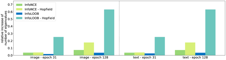
Modern Hopfield networks enable to extract more covariance structure. To demonstrate the effect of modern Hopfield networks, we computed the eigenvalues of the covariance matrix of the image and text embeddings. We counted the number of effective eigenvalues, that is, the number of eigenvalues needed to obtain 99% of the total sum of eigenvalues. Figure 2 shows the relative change of the number of effective eigenvalues compared to the respective reference epoch (the epoch before the first learning rate restart). Modern Hopfield networks consistently increase the number of effective eigenvalues during learning. Consequently, modern Hopfield networks enable to extract more covariance structure during learning, i.e. enrich the embeddings by covariances that are already in the raw multi-modal data. This enrichment of embeddings mitigates explaining away. Further details can be found in Appendix Section A.2.7.

Figure 2: Relative change in the number of the effective eigenvalues of the embedding covariance matrices, which were obtained from image and text encoders at two different training points. Models with modern Hopfield networks steadily extract more covariance structure during learning.

4 InfoLOOB for Contrastive Learning

Modern Hopfield networks lead to a higher similarity of retrieved samples. The increased similarity exacerbates the saturation of the InfoNCE objective. To avoid the saturation of InfoNCE, CLOOB uses the “InfoLOOB” objective. The “InfoLOOB” objective is called “Leave one out upper bound” in Poole et al. (2019) and “L1Out” in Cheng et al. (2020). InfoLOOB is not established as a contrastive objective, although it is a known bound. Recently, InfoLOOB was independently introduced as objective for image-to-image contrastive learning (Yeh et al., 2021).

InfoNCE and InfoLOOB loss functions. $N$ samples are drawn iid from $p(\bm{x},\bm{y})$ giving the training set $\{(\bm{x}_{1},\bm{y}_{1}),\ldots,(\bm{x}_{N},\bm{y}_{N})\}$. For the sample $\bm{y}_{1}$, InfoNCE uses for the matrix of negative samples $\bm{X}=(\bm{x}_{1},\ldots,\bm{x}_{N})$, while InfoLOOB uses $\tilde{\bm{X}}=(\bm{x}_{2},\ldots,\bm{x}_{N})$. The matrices differ by the positive sample $\bm{x}_{1}$. For the score function $f(\bm{x},\bm{y})$, we use $f(\bm{x},\bm{y})=\exp(\tau^{-1}\mathrm{sim}(\bm{x},\bm{y}))$ with the similarity $\mathrm{sim}(\bm{x},\bm{y})=\bm{y}^{T}\bm{x}$ and $\tau$ as the temperature. We have the InfoNCE and InfoLOOB loss functions:

$$\mathrm{L}_{\mathrm{InfoNCE}}\ =\ -\ \frac{1}{N}\sum_{i=1}^{N}\ \ln\frac{\exp(\tau^{-1}\ \bm{x}_{i}^{T}\bm{y}_{i})}{\sum_{j=1}^{N}\exp(\tau^{-1}\ \bm{x}_{i}^{T}\bm{y}_{j})}\ -\ \frac{1}{N}\sum_{i=1}^{N}\ \ln\frac{\exp(\tau^{-1}\ \bm{x}_{i}^{T}\bm{y}_{i})}{\sum_{j=1}^{N}\exp(\tau^{-1}\ \bm{x}_{j}^{T}\bm{y}_{i})}\ ,$$ (7)

$$\mathrm{L}_{\mathrm{InfoLOOB}}\ =\ -\ \frac{1}{N}\sum_{i=1}^{N}\ \ln\frac{\exp(\tau^{-1}\ \bm{x}_{i}^{T}\bm{y}_{i})}{\sum_{j\neq i}^{N}\exp(\tau^{-1}\ \bm{x}_{i}^{T}\bm{y}_{j})}\ -\ \frac{1}{N}\sum_{i=1}^{N}\ \ln\frac{\exp(\tau^{-1}\ \bm{x}_{i}^{T}\bm{y}_{i})}{\sum_{j\neq i}^{N}\exp(\tau^{-1}\ \bm{x}_{j}^{T}\bm{y}_{i})}\ .$$ (8)

We abbreviate $\bm{y}=\bm{y}_{1}$ leading to the pair $(\bm{x}_{1},\bm{y})$ and the negatives $\tilde{\bm{X}}=(\bm{x}_{2},\ldots,\bm{x}_{N})$. In the second sum of the losses in Eq. 7 and Eq. 8, we consider only the first term, respectively:

$$\mathrm{L}_{\mathrm{InfoNCE}}(\bm{y})\ =\ -\ \ln\frac{\color[rgb]{0.27734375,0.72265625,0.67578125}\overbrace{\color[rgb]{0,0,0}\exp(\tau^{-1}\ \bm{x}_{1}^{T}\bm{y})}^{a}}{\color[rgb]{0.27734375,0.72265625,0.67578125}\underbrace{\color[rgb]{0,0,0}\exp(\tau^{-1}\ \bm{x}_{1}^{T}\bm{y})}_{a}\ {\color[rgb]{0,0,0}+}\ \color[rgb]{0.27734375,0.72265625,0.67578125}\underbrace{\color[rgb]{0,0,0}\textstyle{\sum_{j=2}^{N}}\exp(\tau^{-1}\ \bm{x}_{j}^{T}\bm{y})}_{b}}\ ,$$ (9)

$$\mathrm{L}_{\mathrm{InfoLOOB}}(\bm{y})\ =\ -\ \ln\frac{\color[rgb]{0.27734375,0.72265625,0.67578125}\overbrace{\color[rgb]{0,0,0}\exp(\tau^{-1}\ \bm{x}_{1}^{T}\bm{y})}^{a}}{\color[rgb]{0.27734375,0.72265625,0.67578125}\underbrace{\color[rgb]{0,0,0}\textstyle{\sum_{j=2}^{N}}\exp(\tau^{-1}\ \bm{x}_{j}^{T}\bm{y})}_{b}}\ .$$ (10)

In analogy to Wang & Isola (2020), $a$ is called the “alignment score” that measures the similarity of matched pairs and $b$ the “uniformity penalty” that measures the similarity of unmatched pairs.

Gradients of InfoNCE and InfoLOOB loss functions. Eq. (9) and Eq. (10) are equal to

$$-\tau^{-1}\bm{y}^{T}\bm{x}_{1}+\tau^{-1}\mathrm{lse}(\tau^{-1},\bm{X}^{T}\bm{y})\ ,\quad\quad-\tau^{-1}\bm{y}^{T}\bm{x}_{1}+\tau^{-1}\mathrm{lse}(\tau^{-1},\tilde{\bm{X}}^{T}\bm{y})\ ,$$

where $\mathrm{lse}$ is the log-sum-exp function (see Eq. (A73) in the Appendix).

Figure 3: Ajne uniformity test statistics for image and text embeddings for two different epochs during training. A high test statistic indicates low uniformity of an embedding. Models trained with the InfoLOOB objective develop more uniform image and text embeddings on the hypersphere.

The gradients of Eq. (9) and Eq. (10) with respect to $\bm{y}$ are

$$-\tau^{-1}\bm{x}_{1}+\tau^{-1}\bm{X}\mathrm{softmax}(\tau^{-1}\bm{X}^{T}\bm{y})\ ,\quad\quad-\tau^{-1}\bm{x}_{1}+\tau^{-1}\tilde{\bm{X}}\mathrm{softmax}(\tau^{-1}\tilde{\bm{X}}^{T}\bm{y})\ .$$

Using $\bm{p}=(p_{1},\ldots,p_{N})^{T}=\mathrm{softmax}(\tau^{-1}\bm{X}^{T}\bm{y})$, the gradient of InfoNCE with respect to $\bm{y}$ is

$$\frac{\partial\mathrm{L}_{\mathrm{InfoNCE}}(\bm{y})}{\partial\bm{y}}\ =\ -\tau^{-1}(1-p_{1})(\bm{x}_{1}-\tilde{\bm{X}}\mathrm{softmax}(\tau^{-1}\tilde{\bm{X}}^{T}\bm{y}))\ =\ (1-p_{1})\ \frac{\partial\mathrm{L}_{\mathrm{InfoLOOB}}(\bm{y})}{\partial\bm{y}}\ .$$

By and large, the gradient of InfoNCE is scaled by $(1-p_{1})$ compared to the gradient of InfoLOOB, where $p_{1}$ is the softmax similarity between the anchor $\bm{y}$ and the positive sample $\bm{x}_{1}$. Consequently, InfoNCE is saturating with increasing similarity between the anchor and the positive sample. For more details we refer to Appendix Section A.1.4.

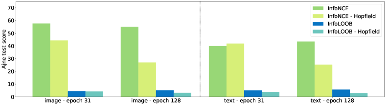
This saturation of InfoNCE motivated the use of the InfoLOOB objective in order to decrease the uniformity penalty even for large alignment scores. The uniformity penalty decreases since learning does not stall and the most prominent features become down-scaled which makes negative examples less similar to the anchor sample. The InfoNCE objective Eq. 9 has the form $a/(a+b)$, while the InfoLOOB objective Eq. 10 has the form $a/b$. InfoLOOB does not saturate and keeps decreasing the uniformity penalty $b$. Figure 3 shows how InfoLOOB leads to an increase in the uniformity of image and text embeddings on the sphere, which is described by the statistics of the uniformity test of Ajne that was extended by Prentice (Ajne, 1968; Prentice, 1978). Higher uniformity on the sphere correlates with a lower uniformity penalty $b$. For more details we refer to Appendix Section A.2.7.

Theoretical justification for optimizing InfoLOOB. The InfoNCE information is a lower bound on the mutual information, which was proven by Poole et al. (2019). In the Appendix Section A.1, we elaborate more on theoretical properties of the bounds and properties of the objective functions. Specifically, we show that InfoLOOB with neural networks is not an upper bound on the mutual information. Thus, unlike hitherto approaches to contrastive learning we use InfoLOOB as an objective, since it does not suffer from saturation effects as InfoNCE.

5 Experiments

CLOOB is compared to CLIP with respect to zero-shot transfer learning performance on two pre-training datasets. The first dataset, Conceptual Captions (CC) (Sharma et al., 2018), has a very rich textual description of images but only three million image-text pairs. The second dataset, a subset of YFCC100M (Thomee et al., 2016), has 15 million image-text pairs but the textual description is less rich than for CC and often vacuous. For both pre-training datasets, the downstream zero-shot transfer learning performance is tested on seven image classification datasets.

5.1 Conceptual Captions Pre-training

Pre-training dataset. The Conceptual Captions (CC) (Sharma et al., 2018) dataset contains 2.9 million images with high-quality captions. Images and their captions have been gathered from the web via an automated process and have a wide variety of content. Raw descriptions of images are from the alt-text HTML attribute.

Methods. The CLOOB implementation is based on OpenCLIP (Ilharco et al., 2021), which achieves results equivalent to CLIP on the YFCC dataset (see Section 5.2). OpenCLIP also reports results on the CC dataset. As CLIP does not train models on CC, we report results from this reimplementation as baseline. Analogously to Radford et al. (2021, Section 2.4), we used the modified ResNet (He et al., 2016) and BERT (Devlin et al., 2018, 2019) architectures to encode image and text input. We used the ResNet encoder ResNet-50 for experiments on CC.

Hyperparameter selection and learning schedule. The hyperparameter values of OpenCLIP were used as default, concretely, a learning rate of $1\times 10^{-3}$ and a weight decay of $0.1$ for the Adam optimizer (Kingma et al., 2014) with decoupled weight decay regularization (Loshchilov & Hutter, 2019). Deviating from OpenCLIP, we used a batch size of $512$ due to computational restraints, which did not change the performance. The learning rate scheduler for all experiments was cosine annealing with warmup and hard restarts (Loshchilov & Hutter, 2017). We report the hyperparameter $\tau$ (default $0.07$) from CLIP as $\tau^{-1}$ of $14.3$ to be in the same regime as the hyperparameter $\beta$ for the modern Hopfield networks. The main hyperparameter search for CLOOB (also for YFCC pre-training in the next section) was done with ResNet-50 as the vision encoder. Learnable $\tau^{-1}$ in combination with the InfoLOOB loss results in undesired learning behavior (see Appendix Section A.1.4). Therefore, we set $\tau^{-1}$ to a fixed value of 30, which was determined via a hyperparameter search (see Appendix Section A.2.2). For modern Hopfield networks, the hyperparameter $\beta$ was set to $8$. Further we scaled the loss $\mathrm{L}_{\mathrm{InfoLOOB}}$ with $\tau$ to remove the factor $\tau^{-1}$ from the gradients (see Appendix Section A.1.4) resulting in the loss function $\tau\mathrm{L}_{\mathrm{InfoLOOB}}$.

Table 1: Zero-shot results for models trained on CC with ResNet-50 vision encoders for two different checkpoints. Results are given as mean accuracy over 5 runs. Statistically significant results are shown in bold. CLIP and CLOOB were trained for 31 epochs while CLIP* and CLOOB* were trained for 128 epochs. In the majority of tasks CLOOB significantly outperforms CLIP.

Dataset	CLIP RN-50	CLOOB RN-50	CLIP* RN-50	CLOOB* RN-50
Birdsnap	2.26 $\pm$ 0.20	3.06 $\pm$ 0.30	2.8 $\pm$ 0.16	3.24 $\pm$ 0.31
Country211	0.67 $\pm$ 0.11	0.67 $\pm$ 0.05	0.7 $\pm$ 0.04	0.73 $\pm$ 0.05
Flowers102	12.56 $\pm$ 0.38	13.45 $\pm$ 1.19	13.32 $\pm$ 0.43	14.36 $\pm$ 1.17
GTSRB	7.66 $\pm$ 1.07	6.38 $\pm$ 2.11	8.96 $\pm$ 1.70	7.03 $\pm$ 1.22
UCF101	20.98 $\pm$ 1.55	22.26 $\pm$ 0.72	21.63 $\pm$ 0.65	23.03 $\pm$ 0.85
Stanford Cars	0.91 $\pm$ 0.10	1.23 $\pm$ 0.10	0.99 $\pm$ 0.16	1.41 $\pm$ 0.32
ImageNet	20.33 $\pm$ 0.28	23.97 $\pm$ 0.15	21.3 $\pm$ 0.42	25.67 $\pm$ 0.22
ImageNet V2	20.24 $\pm$ 0.50	23.59 $\pm$ 0.15	21.24 $\pm$ 0.22	25.49 $\pm$ 0.11

Evaluation metrics: Zero-shot transfer learning. We evaluated and compared both CLIP and CLOOB on their zero-shot transfer learning capabilities on the following downstream image classification tasks. Birdsnap (Berg et al., 2014) contains images of 500 different North American bird species. The Country211 (Radford et al., 2021) dataset consists of photos across 211 countries and is designed to test the geolocalization capability of visual representations. Flowers102 (Nilsback & Zisserman, 2008) is a dataset containing images of 102 flower species. GTSRB (Stallkamp et al., 2011) contains images for classification of German traffic signs. UCF101 (Soomro et al., 2012) is a video dataset with short clips for action recognition. For UCF101 we followed the procedure reported in CLIP and extract the middle frame of every video to assemble the dataset. Stanford Cars (Krause et al., 2013) contains images of 196 types of cars. ImageNet (Deng et al., 2009) is a large scale image classification dataset with images across 1,000 classes. ImageNetv2 (Recht et al., 2019) consists of three new test sets with 10,000 images each for the ImageNet benchmark. For further details see Appendix Section A.2.3.

Results. We employed the same evaluation strategy and used the prompts as published in CLIP (see Appendix Section A.2.3). We report zero-shot results from two checkpoints in Table 1. CLIP and CLOOB were trained for a comparable number of epochs used in CLIP (see Appendix Section A.2.2) while CLIP* and CLOOB* were trained until evaluation performance plateaued (epoch 128). In both cases CLOOB significantly outperforms CLIP on the majority of tasks or matches its performance. Statistical significance of these results was assessed by an unpaired Wilcoxon test on a 5$\%$ level.

5.2 YFCC Pre-training

Pre-training dataset. To be comparable to the CLIP results, we used the same subset of 15 million samples from the YFCC100M dataset (Thomee et al., 2016) as in Radford et al. (2021), which we refer to as YFCC. YFCC was created by filtering YFCC100M for images which contain natural language descriptions and/or titles in English. It was not filtered by quality of the captions, therefore the textual descriptions are less rich and contain superfluous information. The dataset with 400 million samples used to train the CLIP models in Radford et al. (2021) has not been released and, thus, is not available for comparison. Due to limited computational resources we were unable to compare CLOOB to CLIP on other datasets of this size.

Methods. Besides experiments with a ResNet-50 image encoder, we additionally conducted experiments with the larger ResNet variants ResNet-101 and ResNet-50x4. In addition to the comparison of CLOOB and CLIP based on the OpenCLIP reimplementation (Ilharco et al., 2021), we include the original CLIP results (Radford et al., 2021, Table 12).

Hyperparameter selection. Hyperparameters were the same as for the Conceptual Captions dataset, except learning rate, batch size, and $\beta$. For modern Hopfield networks, the hyperparameter $\beta$ was set to $14.3$, which is default for $\tau^{-1}$ in Radford et al. (2021). Furthermore, the learning rate was set to $5\times 10^{-4}$ and the batch size to $1024$ as used in OpenCLIP of Ilharco et al. (2021). All models were trained for 28 epochs. For further details see Appendix Section A.2.2.

Evaluation metrics. As in the previous experiment, methods were again evaluated at their zero-shot transfer learning capabilities on downstream tasks.

Table 2: Results of CLIP and CLOOB trained on YFCC with ResNet-50 encoder. Except for one linear probing dataset, CLOOB consistently outperforms CLIP at all tasks.

	Linear Probing		Zero-Shot
Dataset	CLIP (OpenAI)	CLOOB (ours)	CLIP (OpenAI)	CLOOB (ours)
Birdsnap	47.4	56.2	19.9	28.9
Country211	23.1	20.6	5.2	7.9
Flowers102	94.4	96.1	48.6	55.1
GTSRB	66.8	78.9	6.9	8.1
UCF101	69.2	72.3	22.9	25.3
Stanford Cars	31.4	37.7	3.8	4.1
ImageNet	62.0	65.7	31.3	35.7
ImageNet V2	-	58.7	-	34.6

Table 3: Zero-shot results for the CLIP reimplementation and CLOOB using different ResNet architectures trained on YFCC. CLOOB outperforms CLIP in 7 out of 8 tasks using ResNet-50 encoders. With larger ResNet encoders CLOOB outperforms CLIP on all tasks. The performance of CLOOB scales with increased encoder size.

	RN-50		RN-101		RN-50x4
Dataset	CLIP	CLOOB	CLIP	CLOOB	CLIP	CLOOB
Birdsnap	21.8	28.9	22.6	30.3	20.8	32.0
Country211	6.9	7.9	7.8	8.5	8.1	9.3
Flowers102	48.0	55.1	48.0	55.3	50.1	54.3
GTSRB	7.9	8.1	7.4	11.6	9.4	11.8
UCF101	27.2	25.3	28.6	28.8	31.0	31.9
Stanford Cars	3.7	4.1	3.8	5.5	3.5	6.1
ImageNet	34.6	35.7	35.3	37.1	37.7	39.0
ImageNet V2	33.4	34.6	34.1	35.6	35.9	37.3

Results. Table 2 provides results of the original CLIP and CLOOB trained on YFCC. Results on zero-shot downstream tasks show that CLOOB outperforms CLIP on all 7 tasks (ImageNet V2 results have not been reported in Radford et al. (2021)). Similarly, CLOOB outperforms CLIP on 6 out of 7 tasks for linear probing. Results of CLOOB and the CLIP reimplementation of OpenCLIP are given in Table 3. CLOOB exceeds the CLIP reimplementation in 7 out of 8 tasks for zero-shot classification using ResNet-50 encoders. With larger ResNet encoders, CLOOB outperforms CLIP on all tasks. Furthermore, the experiments with larger vision encoder networks show that CLOOB performance increases with network size. Results of CLOOB zero-shot classification on all datasets are shown in Appendix Section A.2.4.

5.3 Ablation studies

CLOOB has two new major components compared to CLIP: (1) modern Hopfield networks and (2) the InfoLOOB objective instead of the InfoNCE objective. To assess effects of the new major components of CLOOB, we performed ablation studies.

Modern Hopfield networks. Modern Hopfield networks amplify the covariance structure in the data via the retrievals. Ablation studies confirm this amplification as modern Hopfield networks consistently increase the number of effective eigenvalues of the embedding covariance matrices during learning. Figure 2 shows the relative change of the number of effective eigenvalues compared to the respective reference epoch, which is the epoch before the first learning rate restart. These results indicate that modern Hopfield networks steadily extract more covariance structure during learning. Modern Hopfield networks induce higher similarity of retrieved samples, which in turn leads to stronger saturation of the InfoNCE objective. As a result, we observe low uniformity (see Figure 3) and a small number of effective eigenvalues (see Appendix Figure A1).

Modern Hopfield networks with InfoLOOB. CLOOB counters the saturation of InfoNCE by using the InfoLOOB objective. The effectiveness of InfoLOOB manifests in an increased uniformity measure of image and text embeddings on the sphere, as shown in Figure 3. The ablation study verifies that modern Hopfield networks together with InfoLOOB have a strong synergistic effect.

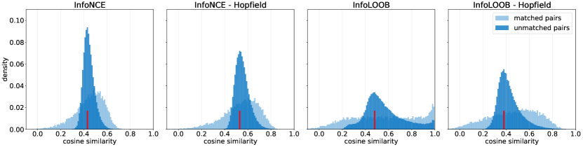
InfoLOOB. However, using solely InfoLOOB results in overfitting of the alignment score. This overfitting occasionally leads to high similarities of unmatched pairs (see Figure 4), which may decreases the zero-shot downstream performance. The reason for this is that the top-1 evaluation metric is very sensitive to occasionally high similarities of prompts of the incorrect class. Yeh et al. (2021) and Zhang et al. (2022) reported similar observations of overfitting.

Figure 4: Distribution of the cosine similarity of matched pairs and the cosine similarity of the 10 unmatched pairs that have the highest similarity score with the anchor. Modern Hopfield networks lead to higher values of both matched and unmatched pairs. InfoLOOB without Hopfield has high similarity scores of the matched pairs which correlate with high similarity scores of the top-10 unmatched pairs. In contrast, InfoLOOB with Hopfield does not suffer from this overfitting problem.

CLOOB balances the overfitting of InfoLOOB with the underfitting of modern Hopfield networks and remains in effective learning regimes. For more details and further ablation studies see Appendix Section A.2.1.

6 Conclusion

We have introduced “Contrastive Leave One Out Boost” (CLOOB), which combines modern Hopfield networks with the InfoLOOB objective. Modern Hopfield networks enable CLOOB to extract additional covariance structure in the data. This allows for building more relevant features in the embedding space, mitigating the explaining away problem. We show that InfoLOOB avoids the saturation problem of InfoNCE. Additionally, we theoretically justify the use of the InfoLOOB objective for contrastive learning and suggest it as an alternative to InfoNCE. At seven zero-shot transfer learning tasks, the novel CLOOB was compared to CLIP after pre-training on the Conceptual Captions and the YFCC dataset. CLOOB consistently outperforms CLIP at zero-shot transfer learning across all considered architectures and datasets.

Checklist

1. For all authors…

   1. Do the main claims made in the abstract and introduction accurately reflect the paper’s contributions and scope? [Yes]

   2. Did you describe the limitations of your work? [Yes] Our method is currently limited to natural images and short text prompts as inputs, and, thus its use for other types of images, such as medical or biological images, is unexplored. While we hypothesize that our approach could also be useful for similar data in other domains, this has not been assessed.

   3. Did you discuss any potential negative societal impacts of your work? [Yes] One potential danger arises from users that overly rely on systems built on our method. For example in the domain of self-driving cars, users might start paying less attention to the traffic because of the AI-based driving system. Finally, our method might also be used to automate various simple tasks, which might lead to reduced need for particular jobs in production systems. As for almost all machine learning methods, our proposed method relies on human-annotated training data and thereby human decisions, which are usually strongly biased. Therefore, the responsible use of our method requires the careful selection of the training data and awareness of potential biases within those.

   4. Have you read the ethics review guidelines and ensured that your paper conforms to them? [Yes]

2. If you are including theoretical results…

   1. Did you state the full set of assumptions of all theoretical results? [Yes]

   2. Did you include complete proofs of all theoretical results? [Yes]

3. If you ran experiments…

   1. Did you include the code, data, and instructions needed to reproduce the main experimental results (either in the supplemental material or as a URL)? [Yes] We provide the URL to a GitHub repository that contains the code.

   2. Did you specify all the training details (e.g., data splits, hyperparameters, how they were chosen)? [Yes] See Section 5.1, Section 5.2 and Appendix Section A.2.2.

   3. Did you report error bars (e.g., with respect to the random seed after running experiments multiple times)? [Yes] We added error bars for all experiments for which this was computationally feasible (see Table 1).

   4. Did you include the total amount of compute and the type of resources used (e.g., type of GPUs, internal cluster, or cloud provider)? [Yes] We used several different servers equipped with GPUs of different types, such as V100 and A100. The total amount of compute is roughly $11,000$ GPU hours (with A100).

4. If you are using existing assets (e.g., code, data, models) or curating/releasing new assets…

   1. If your work uses existing assets, did you cite the creators? [Yes] For the model implementations we used PyTorch (Paszke et al., 2017, BSD license) and for monitoring the runs we used Weights & Biases (Biewald, 2020, MIT license).

   2. Did you mention the license of the assets? [Yes] See above.

   3. Did you include any new assets either in the supplemental material or as a URL? [Yes] We provide the code as supplementary material.

   4. Did you discuss whether and how consent was obtained from people whose data you’re using/curating? [Yes] We only use public datasets that can be used for research purposes, such as the YFCC dataset which was published under the Creative Commons licence.

   5. Did you discuss whether the data you are using/curating contains personally identifiable information or offensive content? [Yes] As almost all computer vision and natural language datasets, the data suffers from many biases including social biases. We refer to Yang et al. (2020) for a detailed analysis of biases in such datasets.

5. If you used crowdsourcing or conducted research with human subjects…

   1. Did you include the full text of instructions given to participants and screenshots, if applicable? [N/A]

   2. Did you describe any potential participant risks, with links to Institutional Review Board (IRB) approvals, if applicable? [N/A]

   3. Did you include the estimated hourly wage paid to participants and the total amount spent on participant compensation? [N/A]

Appendix A Appendix

This appendix consists of four sections (A.1–A.4). Section A.1 provides the theoretical properties of InfoLOOB and InfoNCE. It is shown how to derive that InfoNCE is a lower bound on mutual information. Further it is shown how to derive that InfoLOOB is an upper bound on mutual information. The proposed loss function and its gradients are discussed. Section A.2 provides details on the experiments. Section A.3 briefly reviews continuous modern Hopfield networks. Section A.4 discusses further related work.

Contents of the appendix

1. 1 Introduction
2. 2 CLOOB: Modern Hopfield Networks with InfoLOOB
3. 3 Modern Hopfield Networks for Enriching the Covariance Structure
4. 4 InfoLOOB for Contrastive Learning
5. 5 Experiments
   1. 5.1 Conceptual Captions Pre-training
   2. 5.2 YFCC Pre-training
   3. 5.3 Ablation studies
6. 6 Conclusion
7. A Appendix
   1. A.1 InfoLOOB vs. InfoNCE
      1. A.1.1 InfoNCE: Lower Bound on Mutual Information
      2. A.1.2 InfoLOOB: Upper Bound on Mutual Information
      3. A.1.3 InfoLOOB: Analysis of the Objective
      4. A.1.4 InfoNCE and InfoLOOB: Gradients
      5. A.1.5 InfoLOOB and InfoNCE: Probability Estimators
      6. A.1.6 InfoLOOB and InfoNCE: Losses
   2. A.2 Experiments
      1. A.2.1 Ablation studies
      2. A.2.2 Hyperparameters
      3. A.2.3 Datasets
      4. A.2.4 Zero-shot evaluation
      5. A.2.5 Linear probing
      6. A.2.6 Image-Text retrieval
      7. A.2.7 Analysis of the image and text embeddings
      8. A.2.8 Training time and memory consumption
   3. A.3 Review of Modern Hopfield Networks
   4. A.4 Further Related Work

List of theorems

1. Theorem A1 (InfoNCE lower bound).
2. Theorem A2 (InfoLOOB upper bound).
3. Theorem A3 (Weighted Covariances).
4. Theorem A4 (Modern Hopfield Networks: Retrieval with One Update).
5. Theorem A5 (Modern Hopfield Networks: Exponential Storage Capacity).

List of definitions

1. Definition A1 (Pattern Stored and Retrieved).

List of figures

1. 1 The CLOOB architecture for image-text pairs. The image embedding $\bm{x}_{i}$ and the text embedding $\bm{y}_{i}$ retrieve the embeddings $\bm{U}_{\bm{x}_{i}}$ and $\bm{U}_{\bm{y}_{i}}$, respectively, from a modern Hopfield network that stores image embeddings $\bm{U}=(\bm{u}_{1},\ldots,\bm{u}_{M})$ (green boxes at the left). The image-retrieved image embedding $\bm{U}_{\bm{x}_{i}}$ serves as anchor in order to contrast the positive text-retrieved image embedding $\bm{U}_{\bm{y}_{i}}$ with the negative text-retrieved image embedding $\bm{U}_{\bm{y}_{j}}$ for $j\neq i$. Analogously, for the second modern Hopfield network that stores text embeddings $\bm{V}=(\bm{v}_{1},\ldots,\bm{v}_{K})$ (green boxes at the right).
2. 2 Relative change in the number of the effective eigenvalues of the embedding covariance matrices, which were obtained from image and text encoders at two different training points. Models with modern Hopfield networks steadily extract more covariance structure during learning.
3. 3 Ajne uniformity test statistics for image and text embeddings for two different epochs during training. A high test statistic indicates low uniformity of an embedding. Models trained with the InfoLOOB objective develop more uniform image and text embeddings on the hypersphere.
4. 4 Distribution of the cosine similarity of matched pairs and the cosine similarity of the 10 unmatched pairs that have the highest similarity score with the anchor. Modern Hopfield networks lead to higher values of both matched and unmatched pairs. InfoLOOB without Hopfield has high similarity scores of the matched pairs which correlate with high similarity scores of the top-10 unmatched pairs. In contrast, InfoLOOB with Hopfield does not suffer from this overfitting problem.
5. A1 Eigenvalues of the covariance matrix of image embeddings
6. A2 Distribution of the cosine similarity of matched pairs and the cosine similarity of the 1,000 unmatched pairs that have the highest similarity score with the anchor.
7. A3 Distribution of the cosine similarity of matched pairs and the cosine similarity of the 10 unmatched pairs that have the highest similarity score with the anchor.
8. A4 Visualization of zero-shot classification of three examples from each dataset

List of tables

1. 1 Zero-shot results for models trained on CC with ResNet-50 vision encoders for two different checkpoints. Results are given as mean accuracy over 5 runs. Statistically significant results are shown in bold. CLIP and CLOOB were trained for 31 epochs while CLIP* and CLOOB* were trained for 128 epochs. In the majority of tasks CLOOB significantly outperforms CLIP.
2. 2 Results of CLIP and CLOOB trained on YFCC with ResNet-50 encoder. Except for one linear probing dataset, CLOOB consistently outperforms CLIP at all tasks.
3. 3 Zero-shot results for the CLIP reimplementation and CLOOB using different ResNet architectures trained on YFCC. CLOOB outperforms CLIP in 7 out of 8 tasks using ResNet-50 encoders. With larger ResNet encoders CLOOB outperforms CLIP on all tasks. The performance of CLOOB scales with increased encoder size.
4. A1 Influence of loss functions and Hopfield retrieval (CC)
5. A2 Influence of loss functions and Hopfield retrieval (YFCC)
6. A3 Influence of learning rate scheduler
7. A4 Datasets used for downstream evaluation
8. A5 Zero-shot results for models trained on CC with ResNet-50 vision encoders for two different checkpoints over 20 datasets. Results are given as mean accuracy over 5 runs. Statistically significant results are shown in bold. CLIP and CLOOB were trained for 31 epochs while CLIP* and CLOOB* were trained for 128 epochs.
9. A6 Zero-shot results for the CLIP reimplementation and CLOOB using different ResNet architectures trained on YFCC over 20 datasets.
10. A7 Linear probing for CLIP (reimplementation) and CLOOB trained on YFCC
11. A8 Results for image-to-text and text-to-image retrieval on the CC validation set containing 13,330 samples. Results are given as mean accuracy over 5 runs. Statistically significant results are shown in bold. CLIP and CLOOB were trained for 31 epochs while CLIP* and CLOOB* were trained for 128 epochs.
12. A9 Memory and time consumption of CLIP and CLOOB when trained for 31 epochs on CC.

A.1 InfoLOOB vs. InfoNCE

A.1.1 InfoNCE: Lower Bound on Mutual Information

We derive a lower bound on the mutual information between random variables $X$ and $Y$ distributed according to $p(\bm{x},\bm{y})$. The mutual information $\mathrm{I}(X\;;\;Y)$ between random variables $X$ and $Y$ is

$$\mathrm{I}(X\;;\;Y)\ =\ \mathbf{\mathrm{E}}_{p(\bm{x},\bm{y})}\left[\ln\frac{p(\bm{x},\bm{y})}{p(\bm{x})\ p(\bm{y})}\right]\ =\ \mathbf{\mathrm{E}}_{p(\bm{x},\bm{y})}\left[\ln\frac{p(\bm{x}\mid\bm{y})}{p(\bm{x})}\right]\ =\ \mathbf{\mathrm{E}}_{p(\bm{x},\bm{y})}\left[\ln\frac{p(\bm{y}\mid\bm{x})}{p(\bm{y})}\right]\ .$$ (A1)

“InfoNCE” has been introduced in van den Oord et al. (2018) and is a multi-sample bound. In the setting introduced in van den Oord et al. (2018), we have an anchor sample $\bm{y}$ given. For the anchor sample $\bm{y}$ we draw a positive sample $\bm{x}_{1}$ according to $p(\bm{x}_{1}\mid\bm{y})$. Next, we draw a set $\tilde{X}=\{\bm{x}_{2},\ldots,\bm{x}_{N}\}$ according to $p(\tilde{X})$, which are $n-1$ negative samples drawn iid according to $p(\bm{x})$. We have drawn a set $X=\{\bm{x}_{1},\bm{x}_{2},\ldots,\bm{x}_{N}\}$ according to $p(X\mid\bm{y})$, which is one positive sample $\bm{x}_{1}$ drawn by $p(\bm{x}_{1}\mid\bm{y})$ and $N-1$ negative samples $\{\bm{x}_{2},\ldots,\bm{x}_{N}\}$ drawn iid according to $p(\bm{x})$.

The InfoNCE with probabilities is

$$\mathrm{I}_{\mathrm{#1}}(X_{1}\;;\;Y)\ =\ \mathbf{\mathrm{E}}_{p(\bm{y})}\left[\mathbf{\mathrm{E}}_{p(X\mid\bm{y})}\left[\ln\left(\frac{p(\bm{y}\mid\bm{x}_{1})}{\frac{1}{N}\ \sum_{i=1}^{N}p(\bm{y}\mid\bm{x}_{i})}\right)\right]\right]\ ,$$ (A2)

where we inserted the factor $\frac{1}{N}$ in contrast to the original version in van den Oord et al. (2018), where we followed Poole et al. (2019); Tschannen et al. (2019); Cheng et al. (2020); Chen et al. (2021).

The InfoNCE with score function $f(\bm{x},\bm{y})$ is

$$\mathrm{I}_{\mathrm{#1}}(X_{1}\;;\;Y)\ =\ \mathbf{\mathrm{E}}_{p(\bm{y})}\left[\mathbf{\mathrm{E}}_{p(X\mid\bm{y})}\left[\ln\left(\frac{f(\bm{x}_{1},\bm{y})}{\frac{1}{N}\ \sum_{i=1}^{N}f(\bm{x}_{i},\bm{y})}\right)\right]\right]\ .$$ (A3)

The InfoNCE with probabilities can be rewritten as:

$$\mathrm{I}_{\mathrm{#1}}(X_{1}\;;\;Y)\ =\ \mathbf{\mathrm{E}}_{p(\bm{y})}\left[\mathbf{\mathrm{E}}_{p(X\mid\bm{y})}\left[\ln\left(\frac{p(\bm{y}\mid\bm{x}_{1})}{\frac{1}{N}\ \sum_{i=1}^{N}p(\bm{y}\mid\bm{x}_{i})}\right)\right]\right]$$ (A4)

$$=\ \mathbf{\mathrm{E}}_{p(\bm{y})}\left[\mathbf{\mathrm{E}}_{p(X\mid\bm{y})}\left[\ln\left(\frac{\frac{p(\bm{y}\mid\bm{x}_{1})}{p(\bm{y})}}{\frac{1}{N}\ \sum_{i=1}^{N}\frac{p(\bm{y}\mid\bm{x}_{i})}{p(\bm{y})}}\right)\right]\right]$$

$$=\ \mathbf{\mathrm{E}}_{p(\bm{y})}\left[\mathbf{\mathrm{E}}_{p(X\mid\bm{y})}\left[\ln\left(\frac{\frac{p(\bm{x}_{1}\mid\bm{y})}{p(\bm{x}_{1})}}{\frac{1}{N}\ \sum_{i=1}^{N}\frac{p(\bm{x}_{i}\mid\bm{y})}{p(\bm{x}_{i})}}\right)\right]\right]\ .$$

This is the InfoNCE with $f(\bm{x},\bm{y})=p(\bm{y}\mid\bm{x})$.

Set of pairs. The InfoNCE can be written in a different setting Poole et al. (2019), which is used in most implementations. We sample $N$ pairs independently from $p(\bm{x},\bm{y})$, which gives $Z=\{(\bm{x}_{1},\bm{y}_{1}),(\bm{x}_{2},\bm{y}_{2}),\ldots,(\bm{x}_{N},\bm{y}_{N})\}$. The InfoNCE is then

$$\mathrm{I}_{\mathrm{#1}}(X\;;\;Y)\ =\ \mathbf{\mathrm{E}}_{p(X\mid\bm{y})}\left[\frac{1}{N}\ \sum_{i=1}^{N}\ln\left(\frac{f(\bm{x}_{i},\bm{y}_{i})}{\frac{1}{N}\ \sum_{j=1}^{N}f(\bm{x}_{j},\bm{y}_{i})}\right)\right]\ .$$ (A5)

Following van den Oord et al. (2018) we have

$$\mathrm{I}_{\mathrm{#1}}(X_{1}\;;\;Y)\ =\ \mathbf{\mathrm{E}}_{p(\bm{y})}\left[\mathbf{\mathrm{E}}_{p(X\mid\bm{y})}\left[\ln\left(\frac{\frac{p(\bm{y}\mid\bm{x}_{1})}{p(\bm{y})}}{\frac{1}{N}\ \sum_{i=1}^{N}\frac{p(\bm{y}\mid\bm{x}_{i})}{p(\bm{y})}}\right)\right]\right]$$ (A6)

$$=\ \mathbf{\mathrm{E}}_{p(\bm{y})}\left[\mathbf{\mathrm{E}}_{p(X\mid\bm{y})}\left[\ln\left(\frac{\frac{p(\bm{x}_{1}\mid\bm{y})}{p(\bm{x}_{1})}}{\frac{1}{N}\ \sum_{i=1}^{N}\frac{p(\bm{x}_{i}\mid\bm{y})}{p(\bm{x}_{i})}}\right)\right]\right]$$

$$=\ \mathbf{\mathrm{E}}_{p(\bm{y})}\left[\mathbf{\mathrm{E}}_{p(X\mid\bm{y})}\left[\ln\left(\frac{p(\bm{x}_{1}\mid\bm{y})\ \prod_{l=2}^{N}p(\bm{x}_{l})}{\sum_{i=1}^{N}p(\bm{x}_{i}\mid\bm{y})\ \prod_{l\not=i}p(\bm{x}_{l})}\right)\right]\right]\ +\ \ln(N)$$

$$=\ \mathbf{\mathrm{E}}_{p(\bm{y})}\left[\mathbf{\mathrm{E}}_{p(X\mid\bm{y})}\left[\ln p(i=1\mid X,\bm{y})\right]\right]\ +\ \ln(N)\ ,$$

where $p(i=1\mid X,\bm{y})$ is the probability that sample $\bm{x}_{1}$ is the positive sample if we know there exists exactly one positive sample in $X$.

The InfoNCE is a lower bound on the mutual information. The following inequality is from van den Oord et al. (2018):

$$\mathrm{I}(X_{1}\;;\;Y)\ =\ \mathbf{\mathrm{E}}_{p(\bm{y})}\left[\mathbf{\mathrm{E}}_{p(\bm{x}_{1}\mid\bm{y})}\left[\ln\left(\frac{p(\bm{x}_{1}\mid\bm{y})}{p(\bm{x}_{1})}\right)\right]\right]$$ (A7)

$$=\ \mathbf{\mathrm{E}}_{p(\bm{y})}\left[\mathbf{\mathrm{E}}_{p(\bm{x}_{1}\mid\bm{y})}\left[-\ \ln\left(\frac{p(\bm{x}_{1})}{p(\bm{x}_{1}\mid\bm{y})}\right)\right]\right]$$

$$\geq\ \mathbf{\mathrm{E}}_{p(\bm{y})}\left[\mathbf{\mathrm{E}}_{p(\bm{x}_{1}\mid\bm{y})}\left[-\ \ln\left(\frac{1}{N}\ \ +\ \frac{p(\bm{x}_{1})}{p(\bm{x}_{1}\mid\bm{y})}\right)\right]\right]$$

$$\approx\ \mathbf{\mathrm{E}}_{p(\bm{y})}\left[\mathbf{\mathrm{E}}_{p(X\mid\bm{y})}\left[-\ \ln\left(\frac{1}{N}\ +\ \frac{1}{N}\ \frac{p(\bm{x}_{1})}{p(\bm{x}_{1}\mid\bm{y})}\ \sum_{i=2}^{N}\frac{p(\bm{x}_{i}\mid\bm{y})}{p(\bm{x}_{i})}\right)\right]\right]$$

$$=\ \mathbf{\mathrm{E}}_{p(\bm{y})}\left[\mathbf{\mathrm{E}}_{p(X\mid\bm{y})}\left[\ln\left(\frac{\frac{p(\bm{x}_{1}\mid\bm{y})}{p(\bm{x}_{1})}}{\frac{1}{N}\ \frac{p(\bm{x}_{1}\mid\bm{y})}{p(\bm{x}_{1})}\ +\ \frac{1}{N}\ \sum_{i=2}^{N}\frac{p(\bm{x}_{i}\mid\bm{y})}{p(\bm{x}_{i})}}\right)\right]\right]$$

$$=\ \mathrm{I}_{\mathrm{#1}}(X_{1}\;;\;Y)\ ,$$

where the "$\geq$" is obtained by bounding $\ln(1/N+a)$ by $\ln(a)$, which gives a bound that is not very tight, since $a=\frac{p(\bm{x}_{1})}{p(\bm{x}_{1}\mid\bm{y})}$ can become small. However for the "$\approx$" van den Oord et al. (2018) have to assume

$$\frac{1}{N}\ \sum_{i=2}^{N}\frac{p(\bm{x}_{i}\mid\bm{y})}{p(\bm{x}_{i})}\ =\ \frac{1}{N}\ \sum_{i=2}^{N}\frac{p(\bm{y}\mid\bm{x}_{i})}{p(\bm{y})}\ \geq\ 1\ ,$$ (A8)

which is unclear how to ensure.

For a proof of this bound see Poole et al. (2019).

We assumed that for the anchor sample $\bm{y}$ a positive sample $\bm{x}_{1}$ has been drawn according to $p(\bm{x}_{1}\mid\bm{y})$. A set $\tilde{X}=\{\bm{x}_{2},\ldots,\bm{x}_{N}\}$ of negative samples is drawn according to $p(\bm{x})$. Therefore, we have a set $X=\{\bm{x}_{1},\bm{x}_{2},\ldots,\bm{x}_{N}\}$ that is drawn with one positive sample $\bm{x}_{1}$ and $N-1$ negative samples $\tilde{X}=\{\bm{x}_{2},\ldots,\bm{x}_{N}\}$. We have

$$p(\tilde{X})\ =\ \prod_{i=2}^{N}p(\bm{x}_{i})\ ,$$ (A9)

$$p(X\mid\bm{y})\ =\ p(\bm{x}_{1}\mid\bm{y})\ \prod_{i=2}^{N}p(\bm{x}_{i})\ ,$$ (A10)

$$p(X)\ =\ \prod_{i=1}^{N}p(\bm{x}_{i})\ .$$ (A11)

Next, we present a theorem that shows this bound, where we largely follow Poole et al. (2019) in the proof. In contrast to Poole et al. (2019), we do not use the NWJ bound Nguyen et al. (2010). The mutual information is

$$\mathrm{I}(X_{1}\;;\;Y)\ =\ \mathbf{\mathrm{E}}_{p(\bm{x}_{1},\bm{y})}\left[\ln\left(\frac{p(\bm{x}_{1}\mid\bm{y})}{p(\bm{x}_{1})}\right)\right]\ .$$ (A12)

Theorem A1 (InfoNCE lower bound).

InfoNCE with score function $f(\bm{x},\bm{y})$ according to Eq. (A3) is a lower bound on the mutual information.

$$\mathrm{I}(X_{1}\;;\;Y)\ \geq\ \mathbf{\mathrm{E}}_{p(\bm{y})p(X\mid\bm{y})}\left[\ln\left(\frac{f(\bm{x}_{1},\bm{y})}{\frac{1}{N}\ \sum_{i=1}^{N}f(\bm{x}_{i},\bm{y})}\right)\right]\ =\ \mathrm{I}_{\mathrm{#1}}(X_{1}\;;\;Y)\ .$$ (A13)

InfoNCE with probabilities according to Eq. (A2) is a lower bound on the mutual information.

$$\mathrm{I}(X_{1}\;;\;Y)\ \geq\ \mathbf{\mathrm{E}}_{p(\bm{y})p(X\mid\bm{y})}\left[\ln\left(\frac{p(\bm{y}\mid\bm{x}_{1})}{\frac{1}{N}\ \sum_{i=1}^{N}p(\bm{y}\mid\bm{x}_{i})}\right)\right]\ =\ \mathrm{I}_{\mathrm{#1}}(X_{1}\;;\;Y)\ .$$ (A14)

The second bound Eq. (A14) is a special case of the first bound Eq. (A13).

Proof.

Part (I): Lower bound with score function $f(\bm{x},\bm{y})$.

For each set $\tilde{X}=\{\bm{x}_{2},\ldots,\bm{x}_{N}\}$, we define as data-dependent (depending on $\tilde{X}$) score function $g(\bm{x}_{1},\bm{y},\tilde{X})$ that is based on the score function $f(\bm{x},\bm{y})$. Therefore we have for each $\tilde{X}$ a different data-dependent score function $g$ based on $f$. We will derive a bound on the InfoNCE, which is the expectation of a lower bond on the mutual information over the score functions. For score function $g(\bm{x}_{1},\bm{y},\tilde{X})$, we define a variational distribution $q(\bm{x}_{1}\mid\bm{y},\tilde{X})$ over $\bm{x}_{1}$:

$$q(\bm{x}_{1}\mid\bm{y},\tilde{X})\ =\ \frac{p(\bm{x}_{1})\ g(\bm{x}_{1},\bm{y},\tilde{X})}{Z(\bm{y},\tilde{X})}\ ,$$ (A15)

$$Z(\bm{y},\tilde{X})\ =\ \mathbf{\mathrm{E}}_{p(\bm{x}_{1})}\left[g(\bm{x}_{1},\bm{y},\tilde{X})\right]\ ,$$ (A16)

which ensures

$$\int q(\bm{x}_{1}\mid\bm{y},\tilde{X})\ \mathrm{d}\bm{x}_{1}\ =\ 1\ .$$ (A17)

We have

$$\frac{q(\bm{x}_{1}\mid\bm{y},\tilde{X})}{p(\bm{x}_{1})}\ =\ \frac{g(\bm{x}_{1},\bm{y},\tilde{X})}{Z(\bm{y},\tilde{X})}\ .$$ (A18)

For the function $g$, we set

$$g(\bm{x}_{1},\bm{y},\tilde{X})\ =\ \frac{f(\bm{x}_{1},\bm{y})}{\frac{1}{N}\ \sum_{i=1}^{N}f(\bm{x}_{i},\bm{y})}\ ,$$ (A19)

For the function $f$ we use

$$f(\bm{x}_{1},\bm{y})\ =\ \exp(\tau^{-1}\ \mathrm{sim}(\bm{x}_{1},\bm{y}))\ ,$$ (A20)

where $\mathrm{sim}(\bm{x},\bm{y})$ is typically the cosine similarity.

We next show that InfoNCE is a lower bound on the mutual information.

$$\mathrm{I}(X_{1}\;;\;Y)\ =\ \mathbf{\mathrm{E}}_{p(\tilde{X})}\left[\mathrm{I}(X_{1}\;;\;Y)\right]\ =\ \mathbf{\mathrm{E}}_{p(\tilde{X})}\left[\mathbf{\mathrm{E}}_{p(\bm{x}_{1},\bm{y})}\left[\ln\frac{p(\bm{x}_{1}\mid\bm{y})}{p(\bm{x}_{1})}\right]\right]$$ (A21)

$$=\ \mathbf{\mathrm{E}}_{p(\tilde{X})}\left[\mathbf{\mathrm{E}}_{p(\bm{x}_{1},\bm{y})}\left[\ln\left(\frac{p(\bm{x}_{1}\mid\bm{y})}{q(\bm{x}_{1}\mid\bm{y},\tilde{X})}\ \frac{q(\bm{x}_{1}\mid\bm{y},\tilde{X})}{p(\bm{x}_{1})}\right)\right]\right]$$

$$=\ \mathbf{\mathrm{E}}_{p(\tilde{X})}\left[\mathbf{\mathrm{E}}_{p(\bm{x}_{1},\bm{y})}\left[\ln\frac{q(\bm{x}_{1}\mid\bm{y},\tilde{X})}{p(\bm{x}_{1})}\right]\ +\ \mathbf{\mathrm{E}}_{p(\bm{y})}\left[\mathrm{KL}(p(\bm{x}_{1}\mid\bm{y})\;\|\;q(\bm{x}_{1}\mid\bm{y},\tilde{X}))\right]\right]$$

$$\geq\ \mathbf{\mathrm{E}}_{p(\tilde{X})}\left[\mathbf{\mathrm{E}}_{p(\bm{x}_{1},\bm{y})}\left[\ln\frac{q(\bm{x}_{1}\mid\bm{y},\tilde{X})}{p(\bm{x}_{1})}\right]\right]\ =\ \mathbf{\mathrm{E}}_{p(\tilde{X})}\left[\mathbf{\mathrm{E}}_{p(\bm{x}_{1},\bm{y})}\left[\ln\frac{g(\bm{x}_{1},\bm{y},\tilde{X})}{Z(\bm{y},\tilde{X})}\right]\right]$$

$$=\ \mathbf{\mathrm{E}}_{p(\tilde{X})}\left[\mathbf{\mathrm{E}}_{p(\bm{x}_{1},\bm{y})}\left[\ln g(\bm{x}_{1},\bm{y},\tilde{X})\ -\ \ln\left(\mathbf{\mathrm{E}}_{p(\bm{x}_{1})}\left[g(\bm{x}_{1},\bm{y},\tilde{X})\right]\right)\right]\right]$$

$$=\ \mathbf{\mathrm{E}}_{p(\tilde{X})}\left[\mathbf{\mathrm{E}}_{p(\bm{y})}\left[\mathbf{\mathrm{E}}_{p(\bm{x}_{1}\mid\bm{y})}\left[\ln g(\bm{x}_{1},\bm{y},\tilde{X})\right]\ -\ \ln\left(\mathbf{\mathrm{E}}_{p(\bm{x}_{1})}\left[g(\bm{x}_{1},\bm{y},\tilde{X})\right]\right)\right]\right]$$

$$=\ \mathbf{\mathrm{E}}_{p(\tilde{X})}\left[\mathbf{\mathrm{E}}_{p(\bm{y})}\left[\mathbf{\mathrm{E}}_{p(\bm{x}_{1}\mid\bm{y})}\left[\ln g(\bm{x}_{1},\bm{y},\tilde{X})\right]\right]\right]\ -\ \mathbf{\mathrm{E}}_{p(\tilde{X})}\left[\mathbf{\mathrm{E}}_{p(\bm{y})}\left[\ln\left(\mathbf{\mathrm{E}}_{p(\bm{x}_{1})}\left[g(\bm{x}_{1},\bm{y},\tilde{X})\right]\right)\right]\right]$$

$$\geq\ \mathbf{\mathrm{E}}_{p(\bm{y})p(X\mid\bm{y})}\left[\ln g(\bm{x}_{1},\bm{y},\tilde{X})\right]\ -\ \mathbf{\mathrm{E}}_{p(\tilde{X})}\left[\mathbf{\mathrm{E}}_{p(\bm{y})}\left[\mathbf{\mathrm{E}}_{p(\bm{x}_{1})}\left[g(\bm{x}_{1},\bm{y},\tilde{X})\right]\ -\ 1\right]\right]$$

$$=\ \mathbf{\mathrm{E}}_{p(\bm{y})p(X\mid\bm{y})}\left[\ln\frac{f(\bm{x}_{1},\bm{y})}{\frac{1}{N}\ \sum_{i=1}^{N}f(\bm{x}_{i},\bm{y})}\right]\ -\ \mathbf{\mathrm{E}}_{p(\bm{y})}\left[\mathbf{\mathrm{E}}_{p(X)}\left[\frac{f(\bm{x}_{1},\bm{y})}{\frac{1}{N}\ \sum_{i=1}^{N}f(\bm{x}_{i},\bm{y})}\right]\ -\ 1\right]$$

$$=\ \mathbf{\mathrm{E}}_{p(\bm{y})p(X\mid\bm{y})}\left[\ln\frac{f(\bm{x}_{1},\bm{y})}{\frac{1}{N}\ \sum_{i=1}^{N}f(\bm{x}_{i},\bm{y})}\right]\ -\ \mathbf{\mathrm{E}}_{p(\bm{y})}\left[\frac{1}{N}\ \sum_{i=1}^{N}\mathbf{\mathrm{E}}_{p(X)}\left[\frac{f(\bm{x}_{i},\bm{y})}{\frac{1}{N}\ \sum_{i=1}^{N}f(\bm{x}_{i},\bm{y})}\right]\ -\ 1\right]$$

$$=\ \mathbf{\mathrm{E}}_{p(\bm{y})p(X\mid\bm{y})}\left[\ln\frac{f(\bm{x}_{1},\bm{y})}{\frac{1}{N}\ \sum_{i=1}^{N}f(\bm{x}_{i},\bm{y})}\right]\ -\ \mathbf{\mathrm{E}}_{p(\bm{y})}\left[\mathbf{\mathrm{E}}_{p(X)}\left[\frac{\frac{1}{N}\ \sum_{i=1}^{N}f(\bm{x}_{i},\bm{y})}{\frac{1}{N}\ \sum_{i=1}^{N}f(\bm{x}_{i},\bm{y})}\right]\ -\ 1\right]$$

$$=\ \mathbf{\mathrm{E}}_{p(\bm{y})p(X\mid\bm{y})}\left[\ln\frac{f(\bm{x}_{1},\bm{y})}{\frac{1}{N}\ \sum_{i=1}^{N}f(\bm{x}_{i},\bm{y})}\right]$$

$$=\ \mathrm{I}_{\mathrm{#1}}(X_{1}\;;\;Y)\ .$$

For the first "$\geq$" we used that the Kullback-Leibler divergence is non-negative. For the second "$\geq$" we used the inequality $\ln a\leqslant a-1$ for $a>0$.

Part (II): Lower bound with probabilities.

If the score function $f$ is

$$f(\bm{x},\bm{y})\ =\ p(\bm{y}\mid\bm{x})\ ,$$ (A22)

then the bound is

$$\mathrm{I}(X_{1}\;;\;Y)\ \geq\ \mathbf{\mathrm{E}}_{p(\bm{y})p(X\mid\bm{y})}\left[\ln\left(\frac{f(\bm{x}_{1},\bm{y})}{\frac{1}{N}\ \sum_{i=1}^{N}f(\bm{x}_{i},\bm{y})}\right)\right]\ =\ \mathbf{\mathrm{E}}_{p(\bm{y})p(X\mid\bm{y})}\left[\ln\left(\frac{p(\bm{y}\mid\bm{x}_{1})}{\frac{1}{N}\ \sum_{i=1}^{N}p(\bm{y}\mid\bm{x}_{i})}\right)\right]$$ (A23)

$$=\ \mathbf{\mathrm{E}}_{p(\bm{y})p(X\mid\bm{y})}\left[\ln\left(\frac{\frac{p(\bm{y}\mid\bm{x}_{1})}{p(\bm{y})}}{\frac{1}{N}\ \sum_{i=1}^{N}\frac{p(\bm{y}\mid\bm{x}_{i})}{p(\bm{y})}}\right)\right]\ =\ \mathrm{I}_{\mathrm{#1}}(X_{1}\;;\;Y)\ .$$

This is the bound with probabilities in the theorem. ∎

A.1.2 InfoLOOB: Upper Bound on Mutual Information

We derive an upper bound on the mutual information between random variables $X$ and $Y$ distributed according to $p(\bm{x},\bm{y})$. The mutual information $\mathrm{I}(X\;;\;Y)$ between random variables $X$ and $Y$ is

$$\mathrm{I}(X\;;\;Y)\ =\ \mathbf{\mathrm{E}}_{p(\bm{x},\bm{y})}\left[\ln\frac{p(\bm{x},\bm{y})}{p(\bm{x})\ p(\bm{y})}\right]\ =\ \mathbf{\mathrm{E}}_{p(\bm{x},\bm{y})}\left[\ln\frac{p(\bm{x}\mid\bm{y})}{p(\bm{x})}\right]\ =\ \mathbf{\mathrm{E}}_{p(\bm{x},\bm{y})}\left[\ln\frac{p(\bm{y}\mid\bm{x})}{p(\bm{y})}\right]\ .$$ (A24)

In Poole et al. (2019) Eq. (13) introduces a variational upper bound on the mutual information, which has been called "Leave one out upper bound" (called "L1Out" in Cheng et al. (2020)). For simplicity, we call this bound "InfoLOOB", where LOOB is an acronym for "Leave One Out Bound". In contrast to InfoNCE, InfoLOOB is an upper bound on the mutual information. InfoLOOB is analog to InfoNCE except that the negative samples do not contain a positive sample. Fig. 1 and Fig. 2 in Cheng et al. (2020) both show that InfoLOOB is a better estimator for the mutual information than InfoNCE (van den Oord et al., 2018), MINE (Belghazi et al., 2018), and NWJ (Nguyen et al., 2010).

The InfoLOOB with score function $f(\bm{x},\bm{y})$ is defined as

$$\mathrm{I}_{\mathrm{#1}}(X_{1}\;;\;Y)\ =\ \mathbf{\mathrm{E}}_{p(\bm{y})}\left[\mathbf{\mathrm{E}}_{p(X\mid\bm{y})}\left[\ln\left(\frac{f(\bm{x}_{1},\bm{y})}{\frac{1}{N-1}\ \sum_{i=2}^{N}\ f(\bm{x}_{i},\bm{y})}\right)\right]\right]\ .$$ (A25)

The InfoLOOB with probabilities is defined as

$$\mathrm{I}_{\mathrm{#1}}(X_{1}\;;\;Y)\ =\ \mathbf{\mathrm{E}}_{p(\bm{y})}\left[\mathbf{\mathrm{E}}_{p(X\mid\bm{y})}\left[\ln\left(\frac{p(\bm{y}\mid\bm{x}_{1})}{\frac{1}{N-1}\ \sum_{i=2}^{N}p(\bm{y}\mid\bm{x}_{i})}\right)\right]\right]\ .$$ (A26)

This is the InfoLOOB Eq. (A25) with $f(\bm{x},\bm{y})=p(\bm{y}\mid\bm{x})$.

The InfoLOOB with probabilities can be written in different forms:

$$\mathrm{I}_{\mathrm{#1}}(X_{1}\;;\;Y)\ =\ \mathbf{\mathrm{E}}_{p(\bm{y})}\left[\mathbf{\mathrm{E}}_{p(X\mid\bm{y})}\left[\ln\left(\frac{p(\bm{y}\mid\bm{x}_{1})}{\frac{1}{N-1}\ \sum_{i=2}^{N}p(\bm{y}\mid\bm{x}_{i})}\right)\right]\right]$$ (A27)

$$=\ \mathbf{\mathrm{E}}_{p(\bm{y})}\left[\mathbf{\mathrm{E}}_{p(X\mid\bm{y})}\left[\ln\left(\frac{\frac{p(\bm{y}\mid\bm{x}_{1})}{p(\bm{y})}}{\frac{1}{N-1}\ \sum_{i=2}^{N}\frac{p(\bm{y}\mid\bm{x}_{i})}{p(\bm{y})}}\right)\right]\right]\ =\ \mathbf{\mathrm{E}}_{p(\bm{y})}\left[\mathbf{\mathrm{E}}_{p(X\mid\bm{y})}\left[\ln\left(\frac{\frac{p(\bm{x}_{1}\mid\bm{y})}{p(\bm{x}_{1})}}{\frac{1}{N-1}\ \sum_{i=2}^{N}\frac{p(\bm{x}_{i}\mid\bm{y})}{p(\bm{x}_{i})}}\right)\right]\right]\ .$$

Set of pairs. The InfoLOOB can we written in a different setting (Poole et al., 2019), which will be used in our implementations. We sample $N$ pairs independently from $p(\bm{x},\bm{y})$, which gives $X=\{(\bm{x}_{1},\bm{y}_{1}),(\bm{x}_{2},\bm{y}_{2}),\ldots,(\bm{x}_{N},\bm{y}_{N})\}$. The InfoLOOB is then

$$\mathrm{I}_{\mathrm{#1}}(X\;;\;Y)\ =\ \mathbf{\mathrm{E}}_{p(X\mid\bm{y})}\left[\frac{1}{N}\ \sum_{i=1}^{N}\ln\left(\frac{f(\bm{x}_{i},\bm{y}_{i})}{\frac{1}{N-1}\ \sum_{j=1,j\not=i}^{N}f(\bm{x}_{j},\bm{y}_{i})}\right)\right]\ .$$ (A28)

We assume that an anchor sample $\bm{y}$ is given. For the anchor sample $\bm{y}$ we draw a positive sample $\bm{x}_{1}$ according to $p(\bm{x}_{1}\mid\bm{y})$. Next, we draw a set $\tilde{X}=\{\bm{x}_{2},\ldots,\bm{x}_{N}\}$ of negative samples according to $\tilde{p}(\bm{x}\mid\bm{y})$. For a given $\bm{y}$, the $\bm{x}$ that have a large $p(\bm{x}\mid\bm{y})$ are drawn with a lower probability $\tilde{p}(\bm{x}\mid\bm{y})$ compared to random drawing via $p(\bm{x})$. The negatives are indeed negatives. We have drawn first anchor sample $\bm{y}$ and then $X=\{\bm{x}_{1},\ldots,\bm{x}_{N}\}$, where $\bm{x}_{1}$ is drawn according to $p(\bm{x}_{1}\mid\bm{y})$ and $\tilde{X}=\{\bm{x}_{2},\ldots,\bm{x}_{N}\}$ are drawn iid according to $\tilde{p}(\bm{x}\mid\bm{y})$. We have

$$\tilde{p}(\tilde{X}\mid\bm{y})\ =\ \prod_{i=2}^{N}\tilde{p}(\bm{x}_{i}\mid\bm{y})\ ,$$ (A29)

$$\tilde{p}(X\mid\bm{y})\ =\ p(\bm{x}_{1}\mid\bm{y})\ \prod_{i=2}^{N}\tilde{p}(\bm{x}_{i}\mid\bm{y})\ ,$$ (A30)

$$\tilde{p}(\tilde{X}\mid\bm{y})\ p(\bm{x}_{1})\ =\ p(\bm{x}_{1})\ \prod_{i=2}^{N}\tilde{p}(\bm{x}_{i}\mid\bm{y})\ .$$ (A31)

We assume for score function $f(\bm{x},\bm{y})$

$$\forall_{\bm{y}}\forall_{\bm{x}}:\ \ 0\ <\ f(\bm{x},\bm{y})\ .$$ (A32)

We ensure this by using for score function $f$

$$f(\bm{x},\bm{y})\ =\ \exp(\tau^{-1}\ \mathrm{sim}(\bm{x},\bm{y}))\ ,$$ (A33)

where $\mathrm{sim}(\bm{x},\bm{y})$ is typically the cosine similarity.

InfoLOOB with score function $f(\bm{x},\bm{y})$ and with undersampling via $\tilde{p}(X\mid\bm{y})$ is (compare the definition of InfoLOOB Eq. (A25) without undersampling):

$$\mathrm{I}_{\mathrm{#1}}(X\;;\;Y)\ =\ \mathbf{\mathrm{E}}_{p(\bm{y})}\left[\mathbf{\mathrm{E}}_{\tilde{p}(X\mid\bm{y})}\left[\ln\left(\frac{f(\bm{x}_{1},\bm{y})}{\frac{1}{N-1}\ \sum_{i=2}^{N}\ f(\bm{x}_{i},\bm{y})}\right)\right]\right]\ .$$ (A34)

The reference constant $Z(\bm{y})$ gives the average score $f(\bm{x},\bm{y})$, if the negatives for $\bm{y}$ are selected with lower probability via $\tilde{p}(\bm{x}\mid\bm{y})$ than with random drawing according to $p(\bm{x})$.

$$Z(\bm{y})\ =\ \mathbf{\mathrm{E}}_{\tilde{p}(\bm{x}\mid\bm{y})}\left[f(\bm{x},\bm{y})\right]\ .$$ (A35)

We define the variational distribution

$$q(\bm{x}\mid\bm{y})\ =\ \frac{p(\bm{x})\ f(\bm{x},\bm{y})}{Z^{*}(\bm{y})}\ ,\quad Z^{*}(\bm{y})\ =\ \mathbf{\mathrm{E}}_{p(\bm{x})}\left[f(\bm{x},\bm{y})\right]\ .$$ (A36)

With the variational distribution $q(\bm{x}\mid\bm{y})$, we express our main assumption. The main assumption for the bound is:

$$\mathbf{\mathrm{E}}_{p(\bm{y})}\left[\mathrm{KL}(p(\bm{x}\mid\bm{y})\;\|\;q(\bm{x}\mid\bm{y}))\right]\ \leqslant\ \mathbf{\mathrm{E}}_{p(\bm{y})}\left[\ln Z^{*}(\bm{y})\ -\ \ln Z(\bm{y})\right]\ .$$ (A37)

This assumption can be written as

$$\mathbf{\mathrm{E}}_{p(\bm{y})}\left[\mathbf{\mathrm{E}}_{p(\bm{x}\mid\bm{y})}\left[\ln\left(\frac{p(\bm{y}\mid\bm{x})\ Z(\bm{y})}{p(\bm{y})\ f(\bm{x},\bm{y})}\right)\right]\right]\ \leqslant\ 0\ .$$ (A38)

This assumption ensures that the $\bm{x}$ with large $p(\bm{x}\mid\bm{y})$) are selected with lower probability via $\tilde{p}(\bm{x}\mid\bm{y})$ than with random drawing according to $p(\bm{x})$. The negatives are ensured to be real negatives, that is, $p(\bm{x}\mid\bm{y})$ is small and so is $f(\bm{x},\bm{y})$. Consequently, we make sure that we draw $\bm{x}$ with sufficient small $f(\bm{x},\bm{y})$. The Kullback-Leibler gives the minimal required gap between drawing $f(\bm{x},\bm{y})$ via $p(\bm{x})$ and drawing $f(\bm{x},\bm{y})$ via $\tilde{p}(\bm{x}\mid\bm{y})$.

EXAMPLE. With $h(\bm{y})>0$, we consider the setting

$$f(\bm{x},\bm{y})\ =\ \frac{p(\bm{y}\mid\bm{x})\ h(\bm{y})}{p(\bm{y})}\ ,$$ (A39)

$$\tilde{p}(\bm{x}\mid\bm{y})\ =\ \frac{p(\bm{x})\ p(\bm{y})}{h(\bm{y})\ p(\bm{y}\mid\bm{x})\ C(\bm{y})}\ ,\quad C(\bm{y})\ =\ \mathbf{\mathrm{E}}_{p(\bm{x})}\left[\left(\frac{p(\bm{y}\mid\bm{x})\ h(\bm{y})}{p(\bm{y})}\right)^{-1}\right]\ .$$ (A40)

The main assumption becomes

$$\mathbf{\mathrm{E}}_{p(\bm{y})}\left[\mathbf{\mathrm{E}}_{p(\bm{x}\mid\bm{y})}\left[\ln\frac{Z(\bm{y})}{h(\bm{y})}\right]\right]\ \leqslant\ 0\ .$$ (A41)

The main assumption holds since

$$Z(\bm{y})\ =\ \mathbf{\mathrm{E}}_{\tilde{p}(\bm{x}\mid\bm{y})}\left[\frac{p(\bm{y}\mid\bm{x})\ h(\bm{y})}{p(\bm{y})}\right]\ =\ \int\frac{p(\bm{x})\ p(\bm{y})}{h(\bm{y})\ p(\bm{y}\mid\bm{x})\ C(\bm{y})}\ \frac{p(\bm{y}\mid\bm{x})\ h(\bm{y})}{p(\bm{y})}\ \mathrm{d}\bm{x}$$ (A42)

$$=\ \int p(\bm{x})\ C(\bm{y})^{-1}\ \mathrm{d}\bm{x}\ =\ C(\bm{y})^{-1}\ =\ \left(\mathbf{\mathrm{E}}_{p(\bm{x})}\left[\left(\frac{p(\bm{y}\mid\bm{x})\ h(\bm{y})}{p(\bm{y})}\right)^{-1}\right]\right)^{-1}$$

$$\leqslant\ \left(\mathbf{\mathrm{E}}_{p(\bm{x})}\left[\frac{p(\bm{y}\mid\bm{x})\ h(\bm{y})}{p(\bm{y})}\right]^{-1}\right)^{-1}\ =\ \mathbf{\mathrm{E}}_{p(\bm{x})}\left[\frac{p(\bm{y}\mid\bm{x})\ h(\bm{y})}{p(\bm{y})}\right]$$

$$=\ \int\frac{p(\bm{y},\bm{x})\ h(\bm{y})}{p(\bm{y})}\ \mathrm{d}\bm{x}\ =\ h(\bm{y})\ ,$$

where we used for the $\leqslant$ Jensen’s inequality with the function $f(a)=1/a$, which is convex for $a>0$.

For score function $f(\bm{x},\bm{y})$ and distribution $\tilde{p}(\bm{x}\mid\bm{y})$ for sampling the negative samples, we have defined:

$$Z(\bm{y})\ =\ \mathbf{\mathrm{E}}_{\tilde{p}(\bm{x}\mid\bm{y})}\left[f(\bm{x},\bm{y})\right]\ ,$$ (A43)

$$Z^{*}(\bm{y})\ =\ \mathbf{\mathrm{E}}_{p(\bm{x})}\left[f(\bm{x},\bm{y})\right]\ ,$$ (A44)

$$q(\bm{x}\mid\bm{y})\ =\ \frac{p(\bm{x})\ f(\bm{x},\bm{y})}{Z^{*}(\bm{y})}\ .$$ (A45)

Next theorem gives the upper bound of the InfoLOOB on the mutual information, which is

$$\mathrm{I}(X_{1}\;;\;Y)\ =\ \mathbf{\mathrm{E}}_{p(\bm{x}_{1},\bm{y})}\left[\ln\frac{p(\bm{x}_{1}\mid\bm{y})}{p(\bm{x}_{1})}\right]\ .$$ (A46)

Theorem A2 (InfoLOOB upper bound).

If $\tilde{X}=\{\bm{x}_{2},\ldots,\bm{x}_{N}\}$ are drawn iid according to $\tilde{p}(\bm{x}\mid\bm{y})$ and if the main assumption holds:

$$\mathbf{\mathrm{E}}_{p(\bm{y})}\left[\mathrm{KL}(p(\bm{x}\mid\bm{y})\;\|\;q(\bm{x}\mid\bm{y}))\right]\ \leqslant\ \mathbf{\mathrm{E}}_{p(\bm{y})}\left[\ln Z^{*}(\bm{y})\ -\ \ln Z(\bm{y})\right]\ .$$ (A47)

Then InfoLOOB with score function $f(\bm{x},\bm{y})$ and undersampling positives by $\tilde{p}(X\mid\bm{y})$ is an upper bound on the mutual information:

$$\mathrm{I}(X_{1}\;;\;Y)\ \leqslant\ \mathbf{\mathrm{E}}_{p(\bm{y})}\left[\mathbf{\mathrm{E}}_{\tilde{p}(X\mid\bm{y})}\left[\ln\left(\frac{f(\bm{x}_{1},\bm{y})}{\frac{1}{N-1}\ \sum_{i=2}^{N}\ f(\bm{x}_{i},\bm{y})}\right)\right]\right]\ =\ \mathrm{I}_{\mathrm{#1}}(X_{1}\;;\;Y)\ .$$ (A48)

If the negative samples $\tilde{X}=\{\bm{x}_{2},\ldots,\bm{x}_{N}\}$ are drawn iid according to $p(\bm{x})$, then InfoLOOB with probabilities according to Eq. (A26) is an upper bound on the mutual information:

$$\mathrm{I}(X_{1}\;;\;Y)\ \leqslant\ \mathbf{\mathrm{E}}_{p(\bm{y})}\left[\mathbf{\mathrm{E}}_{p(X\mid\bm{y})}\left[\ln\left(\frac{p(\bm{y}\mid\bm{x}_{1})}{\frac{1}{N-1}\ \sum_{i=2}^{N}p(\bm{y}\mid\bm{X}_{i})}\right)\right]\right]\ =\ \mathrm{I}_{\mathrm{#1}}(X_{1}\;;\;Y)\ .$$ (A49)

The second bound Eq. (A49) is a special case of the first bound Eq. (A48).

Proof.

Part (I): Upper bound with score function $f(\bm{x},\bm{y})$.

$$\mathrm{I}(X_{1}\;;\;Y)\ =\ \mathbf{\mathrm{E}}_{p(\bm{x}_{1},\bm{y})}\left[\ln\frac{p(\bm{x}_{1}\mid\bm{y})}{p(\bm{x}_{1})}\right]$$ (A50)

$$=\ \mathbf{\mathrm{E}}_{p(\bm{x}_{1},\bm{y})}\left[\ln\left(\frac{p(\bm{x}_{1}\mid\bm{y})}{q(\bm{x}_{1}\mid\bm{y})}\ \frac{q(\bm{x}_{1}\mid\bm{y})}{p(\bm{x}_{1})}\right)\right]$$

$$=\ \mathbf{\mathrm{E}}_{p(\bm{x}_{1},\bm{y})}\left[\ln\frac{q(\bm{x}_{1}\mid\bm{y})}{p(\bm{x}_{1})}\right]\ +\ \mathbf{\mathrm{E}}_{p(\bm{y})}\left[\mathrm{KL}(p(\bm{x}_{1}\mid\bm{y})\;\|\;q(\bm{x}_{1}\mid\bm{y}))\right]$$

$$\leqslant\ \mathbf{\mathrm{E}}_{p(\bm{x}_{1},\bm{y})}\left[\ln\frac{q(\bm{x}_{1}\mid\bm{y})}{p(\bm{x}_{1})}\right]\ +\ \mathbf{\mathrm{E}}_{p(\bm{y})}\left[\ln\mathbf{\mathrm{E}}_{p(\bm{x}_{1})}\left[f(\bm{x}_{1},\bm{y})\right]\ -\ \ln Z(\bm{y})\right]$$

$$=\ \mathbf{\mathrm{E}}_{p(\bm{x}_{1},\bm{y})}\left[\ln\frac{q(\bm{x}_{1}\mid\bm{y})}{p(\bm{x}_{1})}\ +\ \ln\frac{\mathbf{\mathrm{E}}_{p(\bm{x}_{1})}\left[f(\bm{x}_{1},\bm{y})\right]}{Z(\bm{y})}\right]$$

$$=\ \mathbf{\mathrm{E}}_{p(\bm{x}_{1},\bm{y})}\left[\ln\left(\frac{f(\bm{x}_{1},\bm{y})}{\mathbf{\mathrm{E}}_{p(\bm{x}_{1})}\left[f(\bm{x}_{1},\bm{y})\right]}\ \frac{\mathbf{\mathrm{E}}_{p(\bm{x}_{1})}\left[f(\bm{x}_{1},\bm{y})\right]}{Z(\bm{y})}\right)\right]$$

$$=\ \mathbf{\mathrm{E}}_{p(\bm{x}_{1},\bm{y})}\left[\ln\frac{f(\bm{x}_{1},\bm{y})}{Z(\bm{y})}\right]$$

$$=\ \mathbf{\mathrm{E}}_{p(\bm{x}_{1},\bm{y})}\left[\ln\left(\frac{f(\bm{x}_{1},\bm{y})}{\mathbf{\mathrm{E}}_{\tilde{p}(X\mid\bm{y})}\left[\frac{1}{N-1}\ \sum_{i=2}^{N}\ f(\bm{x}_{i},\bm{y})\right]}\ \right)\right]$$

$$=\ \mathbf{\mathrm{E}}_{p(\bm{x}_{1},\bm{y})}\left[\ln f(\bm{x}_{1},\bm{y})\right]\ -\ \mathbf{\mathrm{E}}_{p(\bm{y})}\left[\ln\left(\mathbf{\mathrm{E}}_{\tilde{p}(X\mid\bm{y})}\left[\frac{1}{N-1}\ \sum_{i=2}^{N}\ f(\bm{x}_{i},\bm{y})\right]\right)\right]$$

$$\leqslant\ \mathbf{\mathrm{E}}_{p(\bm{x}_{1},\bm{y})}\left[\ln f(\bm{x}_{1},\bm{y})\right]\ -\ \mathbf{\mathrm{E}}_{p(\bm{y})}\left[\mathbf{\mathrm{E}}_{\tilde{p}(X\mid\bm{y})}\left[\ln\left(\frac{1}{N-1}\ \sum_{i=2}^{N}\ f(\bm{x}_{i},\bm{y})\right)\right]\right]$$

$$=\ \mathbf{\mathrm{E}}_{p(\bm{y})}\left[\mathbf{\mathrm{E}}_{\tilde{p}(X\mid\bm{y})}\left[\ln\left(\frac{f(\bm{x}_{1},\bm{y})}{\frac{1}{N-1}\ \sum_{i=2}^{N}\ f(\bm{x}_{i},\bm{y})}\right)\right]\right]$$

$$=\ \mathrm{I}_{\mathrm{#1}}(X_{1}\;;\;Y)\ ,$$

where the first "$\leqslant$" uses assumption Eq. (A37), while Jensens’s inequality was used for the second "$\leqslant$" by exchanging the expectation and the "$\ln$". We also used

$$\mathbf{\mathrm{E}}_{\tilde{p}(X\mid\bm{y})}\left[\frac{1}{N-1}\ \sum_{i=2}^{N}\ f(\bm{x}_{i},\bm{y})\right]\ =\ \frac{1}{N-1}\ \sum_{i=2}^{N}\mathbf{\mathrm{E}}_{\tilde{p}(\bm{x}_{i}\mid\bm{y})}\left[f(\bm{x}_{i},\bm{y})\right]\ =\ \frac{1}{N-1}\ \sum_{i=2}^{N}Z(\bm{y})\ =\ Z(\bm{y})\ .$$ (A51)

Part (II): Upper bound with probabilities.

If the score function $f$ is

$$f(\bm{x},\bm{y})\ =\ p(\bm{y}\mid\bm{x})$$ (A52)

and

$$\tilde{p}(\bm{x}\mid\bm{y})\ =\ p(\bm{x})\ ,$$ (A53)

then

$$\tilde{p}(X\mid\bm{y})\ =\ p(X\mid\bm{y})\ ,$$ (A54)

$$Z(\bm{y})\ =\ \mathbf{\mathrm{E}}_{p(\bm{x})}\left[p(\bm{y}\mid\bm{x})\right]\ =\ p(\bm{y})\ ,$$ (A55)

$$Z^{*}(\bm{y})\ =\ \mathbf{\mathrm{E}}_{p(\bm{x})}\left[p(\bm{y}\mid\bm{x})\right]\ =\ p(\bm{y})\ ,$$ (A56)

$$q(\bm{x}\mid\bm{y})\ =\ \frac{p(\bm{x})\ p(\bm{y}\mid\bm{x})}{p(\bm{y})}\ =\ p(\bm{x}\mid\bm{y})\ ,$$ (A57)

$$\mathrm{KL}(p(\bm{x}\mid\bm{y})\;\|\;q(\bm{x}\mid\bm{y}))\ =\ \mathrm{KL}(p(\bm{x}\mid\bm{y})\;\|\;p(\bm{x}\mid\bm{y}))\ =\ 0\ .$$ (A58)

Therefore, the main assumption holds, since

$$0\ =\ \mathbf{\mathrm{E}}_{p(\bm{y})}\left[\mathrm{KL}(p(\bm{x}\mid\bm{y})\;\|\;q(\bm{x}\mid\bm{y}))\right]\ =\ \mathbf{\mathrm{E}}_{p(\bm{y})}\left[\ln Z^{*}(\bm{y})\ -\ \ln Z(\bm{y})\right]\ .$$ (A59)

The bound becomes

$$\mathrm{I}(X_{1}\;;\;Y)\ \leqslant\ \mathbf{\mathrm{E}}_{p(\bm{y})}\left[\mathbf{\mathrm{E}}_{p(X\mid\bm{y})}\left[\ln\left(\frac{p(\bm{y}\mid\bm{x}_{1})}{\frac{1}{N-1}\ \sum_{i=2}^{N}\ p(\bm{y}\mid\bm{x}_{i})}\right)\right]\right]$$ (A60)

$$=\ \mathbf{\mathrm{E}}_{p(\bm{y})}\left[\mathbf{\mathrm{E}}_{p(X\mid\bm{y})}\left[\ln\left(\frac{\frac{p(\bm{y}\mid\bm{x}_{1})}{p(\bm{y})}}{\frac{1}{N-1}\ \sum_{i=2}^{N}\ \frac{p(\bm{y}\mid\bm{x}_{i})}{p(\bm{y})}}\right)\right]\right]\ =\ \mathrm{I}_{\mathrm{#1}}(X_{1}\;;\;Y)\ .$$

An alternative proof is as follows:

$$\mathrm{I}(X_{1}\;;\;Y)\ =\ \mathrm{I}(X_{1}\;;\;Y)\ -\ \mathbf{\mathrm{E}}_{p(\bm{y})}\left[\ln\left(\frac{1}{N-1}\ \sum_{i=2}^{N}\frac{p(\bm{y})}{p(\bm{y})}\right)\right]$$ (A61)

$$=\ \mathrm{I}(X_{1}\;;\;Y)\ -\ \mathbf{\mathrm{E}}_{p(\bm{y})}\left[\ln\left(\mathbf{\mathrm{E}}_{p(X\mid\bm{y})}\left[\frac{1}{N-1}\ \sum_{i=2}^{N}\frac{p(\bm{y}\mid\bm{x}_{i})}{p(\bm{y})}\right]\right)\right]$$

$$\leqslant\ \mathrm{I}(X_{1}\;;\;Y)\ -\ \mathbf{\mathrm{E}}_{p(\bm{y})}\left[\mathbf{\mathrm{E}}_{p(X\mid\bm{y})}\left[\ln\left(\frac{1}{N-1}\ \sum_{i=2}^{N}\frac{p(\bm{y}\mid\bm{x}_{i})}{p(\bm{y})}\right)\right]\right]$$

$$=\ \mathbf{\mathrm{E}}_{p(\bm{y})}\left[\mathbf{\mathrm{E}}_{p(\bm{x}_{1}\mid\bm{y})}\left[\ln\left(\frac{p(\bm{x}_{1}\mid\bm{y})}{p(\bm{x}_{1})}\right)\right]\right]\ -\ \mathbf{\mathrm{E}}_{p(\bm{y})}\left[\mathbf{\mathrm{E}}_{p(X\mid\bm{y})}\left[\ln\left(\frac{1}{N-1}\ \sum_{i=2}^{N}\frac{p(\bm{x}_{i}\mid\bm{y})}{p(\bm{x}_{i})}\right)\right]\right]$$

$$=\ \mathbf{\mathrm{E}}_{p(\bm{y})}\left[\mathbf{\mathrm{E}}_{p(X\mid\bm{y})}\left[\ln\left(\frac{\frac{p(\bm{x}_{1}\mid\bm{y})}{p(\bm{x}_{1})}}{\frac{1}{N-1}\ \sum_{i=2}^{N}\frac{p(\bm{x}_{i}\mid\bm{y})}{p(\bm{x}_{i})}}\right)\right]\right]$$

$$=\ \mathrm{I}_{\mathrm{#1}}(X_{1}\;;\;Y)\ .$$

where we applied Jensens’s inequality for the exchanging the expectation and the "$\ln$" to obtain the "$\leqslant$" inequality.

∎

Experiments that compare upper and lower bounds as mutual information estimates are provided in Cheng et al. (2020) and in Poole et al. (2019). In Fig. 2 in Cheng et al. (2020) it is shown that InfoLOOB is a good estimator of the mutual information.

A.1.3 InfoLOOB: Analysis of the Objective

This subsection justifies the maximization of the InfoLOOB bound for contrastive learning. Maximizing the InfoLOOB bound is not intuitive as it was introduced as an upper bound on the mutual information in the previous subsection. Still maximizing the InfoLOOB bound leads to a good approximation of the mutual information, in particular for high mutual information.

InfoLOOB with a neural network as a scoring function is not an upper bound on the mutual information when not under-sampling. As we use InfoLOOB on training data for which we do not know the sampling procedure, we cannot assume under-sampling. Therefore, we elaborate more on the rationale behind the maximization of the InfoLOOB bound. (I) We show that InfoLOOB with neural networks as scoring function is bounded from above. Therefore, there exists a maximum and the optimization problem is well defined. (II) We show that InfoLOOB with neural networks as scoring function differs by two terms from the mutual information. The first term is the Kullback-Leibler divergence between the variational $q(\bm{x}\mid\bm{y})$ and the posterior $p(\bm{x}\mid\bm{y})$. This divergence is minimal for $q(\bm{x}\mid\bm{y})=p(\bm{x}\mid\bm{y})$, which implies $f(\bm{y}\mid\bm{x})=p(\bm{y}\mid\bm{x})$. The second term is governed by the difference between the mean $\mathbf{\mathrm{E}}[f(\bm{x},\bm{y})]$ and the empirical mean $1/(N-1)\sum_{i}f(\bm{x}_{i},\bm{y})$. The Hoeffding bound can be applied to this difference. Therefore, the second term is negligible for large $N$. In contrast, the KL term is dominant and the relevant term, therefore maximizing InfoLOOB leads to $f(\bm{y}\mid\bm{x})\approx p(\bm{y}\mid\bm{x})$.

We assume that an anchor sample $\bm{y}$ is given. For the anchor sample $\bm{y}$, we draw a positive sample $\bm{x}_{1}$ according to $p(\bm{x}_{1}\mid\bm{y})$. We define the set $\tilde{X}=\{\bm{x}_{2},\ldots,\bm{x}_{N}\}$ of negative samples, which are drawn iid according to $p(\bm{x})$. We define the set $X=\{\bm{x}_{1},\ldots,\bm{x}_{N}\}$.

We have

$$p(\tilde{X})\ =\ \prod_{i=2}^{N}p(\bm{x}_{i})\ ,$$ (A62)

$$p(X\mid\bm{y})\ =\ p(\bm{x}_{1}\mid\bm{y})\ \prod_{i=2}^{N}p(\bm{x}_{i})\ =\ p(\bm{x}_{1}\mid\bm{y})\ p(\tilde{X})\ ,$$ (A63)

$$p(X)\ =\ \prod_{i=1}^{N}p(\bm{x}_{i})\ =\ p(\bm{x}_{1})\ p(\tilde{X})\ .$$ (A64)

We use the score function

$$f(\bm{x},\bm{y})\ =\ \exp(\tau^{-1}\ \mathrm{sim}(\bm{x},\bm{y}))\ ,$$ (A65)

where $\mathrm{sim}(\bm{x},\bm{y})$ is typically the cosine similarity.

The InfoLOOB with score function $f(\bm{x},\bm{y})$ is defined as

$$\mathrm{I}_{\mathrm{#1}}(X_{1}\;;\;Y)\ =\ \mathbf{\mathrm{E}}_{p(\bm{y})}\left[\mathbf{\mathrm{E}}_{p(X\mid\bm{y})}\left[\ln\left(\frac{f(\bm{x}_{1},\bm{y})}{\frac{1}{N-1}\ \sum_{i=2}^{N}\ f(\bm{x}_{i},\bm{y})}\right)\right]\right]\ .$$ (A66)

We define the variational distribution

$$q(\bm{x}\mid\bm{y})\ =\ \frac{p(\bm{x})\ f(\bm{x},\bm{y})}{Z(\bm{y})}\ ,$$ (A67)

$$Z(\bm{y})\ =\ \mathbf{\mathrm{E}}_{p(\bm{x})}\left[f(\bm{x},\bm{y})\right]\ .$$ (A68)

The next inequality shows the relation between $\mathrm{I}(X_{1}\;;\;Y)$ and $\mathrm{I}_{\mathrm{#1}}(X_{1}\;;\;Y)$ for random variables $X_{1}$ and $Y$.

$$\mathrm{I}(X_{1}\;;\;Y)\ =\ \mathbf{\mathrm{E}}_{p(\bm{x}_{1},\bm{y})}\left[\ln\frac{p(\bm{x}_{1}\mid\bm{y})}{p(\bm{x}_{1})}\right]$$ (A69)

$$=\ \mathbf{\mathrm{E}}_{p(\bm{x}_{1},\bm{y})}\left[\ln\left(\frac{p(\bm{x}_{1}\mid\bm{y})}{q(\bm{x}_{1}\mid\bm{y})}\ \frac{q(\bm{x}_{1}\mid\bm{y})}{p(\bm{x}_{1})}\right)\right]$$

$$=\ \mathbf{\mathrm{E}}_{p(\bm{x}_{1},\bm{y})}\left[\ln\frac{q(\bm{x}_{1}\mid\bm{y})}{p(\bm{x}_{1})}\right]\ +\ \mathbf{\mathrm{E}}_{p(\bm{y})}\left[\mathrm{KL}(p(\bm{x}_{1}\mid\bm{y})\;\|\;q(\bm{x}_{1}\mid\bm{y}))\right]$$

$$=\ \mathbf{\mathrm{E}}_{p(\bm{x}_{1},\bm{y})}\left[\ln\frac{f(\bm{x}_{1},\bm{y})}{Z(\bm{y})}\right]\ +\ \mathbf{\mathrm{E}}_{p(\bm{y})}\left[\mathrm{KL}(p(\bm{x}_{1}\mid\bm{y})\;\|\;q(\bm{x}_{1}\mid\bm{y}))\right]$$

$$=\ \mathbf{\mathrm{E}}_{p(\bm{x}_{1},\bm{y})}\left[\ln\left(\frac{f(\bm{x}_{1},\bm{y})}{\mathbf{\mathrm{E}}_{p(X\mid\bm{y})}\left[\frac{1}{N-1}\ \sum_{i=2}^{N}\ f(\bm{x}_{i},\bm{y})\right]}\ \right)\right]\ +\ \mathbf{\mathrm{E}}_{p(\bm{y})}\left[\mathrm{KL}(p(\bm{x}_{1}\mid\bm{y})\;\|\;q(\bm{x}_{1}\mid\bm{y}))\right]$$

$$=\ \mathbf{\mathrm{E}}_{p(\bm{x}_{1},\bm{y})}\left[\ln f(\bm{x}_{1},\bm{y})\right]\ -\ \mathbf{\mathrm{E}}_{p(\bm{y})}\left[\ln\left(\mathbf{\mathrm{E}}_{p(X\mid\bm{y})}\left[\frac{1}{N-1}\ \sum_{i=2}^{N}\ f(\bm{x}_{i},\bm{y})\right]\right)\right]$$

$$+\ \mathbf{\mathrm{E}}_{p(\bm{y})}\left[\mathrm{KL}(p(\bm{x}_{1}\mid\bm{y})\;\|\;q(\bm{x}_{1}\mid\bm{y}))\right]$$

$$=\ \mathbf{\mathrm{E}}_{p(\bm{x}_{1},\bm{y})}\left[\ln f(\bm{x}_{1},\bm{y})\right]\ -\ \mathbf{\mathrm{E}}_{p(\bm{y})}\left[\mathbf{\mathrm{E}}_{p(X\mid\bm{y})}\left[\ln\left(\frac{1}{N-1}\ \sum_{i=2}^{N}\ f(\bm{x}_{i},\bm{y})\right)\right]\right]$$

$$+\ \mathbf{\mathrm{E}}_{p(\bm{y})}\left[\mathbf{\mathrm{E}}_{p(X\mid\bm{y})}\left[\ln\left(\frac{1}{N-1}\ \sum_{i=2}^{N}\ f(\bm{x}_{i},\bm{y})\right)\right]\right]\ -\ \mathbf{\mathrm{E}}_{p(\bm{y})}\left[\ln\left(\mathbf{\mathrm{E}}_{p(X\mid\bm{y})}\left[\frac{1}{N-1}\ \sum_{i=2}^{N}\ f(\bm{x}_{i},\bm{y})\right]\right)\right]$$

$$+\ \mathbf{\mathrm{E}}_{p(\bm{y})}\left[\mathrm{KL}(p(\bm{x}_{1}\mid\bm{y})\;\|\;q(\bm{x}_{1}\mid\bm{y}))\right]$$

$$=\ \mathbf{\mathrm{E}}_{p(\bm{y})}\left[\mathbf{\mathrm{E}}_{p(X\mid\bm{y})}\left[\ln\left(\frac{f(\bm{x}_{1},\bm{y})}{\frac{1}{N-1}\ \sum_{i=2}^{N}\ f(\bm{x}_{i},\bm{y})}\right)\right]\right]\ +\ \mathbf{\mathrm{E}}_{p(\bm{y})}\left[\mathbf{\mathrm{E}}_{p(X\mid\bm{y})}\left[\ln\left(\frac{1}{N-1}\ \sum_{i=2}^{N}\ f(\bm{x}_{i},\bm{y})\right)\right]\right]$$

$$-\ \mathbf{\mathrm{E}}_{p(\bm{y})}\left[\ln\left(\mathbf{\mathrm{E}}_{p(X\mid\bm{y})}\left[\frac{1}{N-1}\ \sum_{i=2}^{N}\ f(\bm{x}_{i},\bm{y})\right]\right)\right]\ +\ \mathbf{\mathrm{E}}_{p(\bm{y})}\left[\mathrm{KL}(p(\bm{x}_{1}\mid\bm{y})\;\|\;q(\bm{x}_{1}\mid\bm{y}))\right]$$

$$=\ \mathrm{I}_{\mathrm{#1}}(X_{1}\;;\;Y)$$

$$+\ \mathbf{\mathrm{E}}_{p(\bm{y})}\left[\mathbf{\mathrm{E}}_{p(X\mid\bm{y})}\left[\ln\left(\frac{1}{N-1}\ \sum_{i=2}^{N}\ f(\bm{x}_{i},\bm{y})\right)\right]\right]\ -\ \mathbf{\mathrm{E}}_{p(\bm{y})}\left[\ln\left(\mathbf{\mathrm{E}}_{p(X\mid\bm{y})}\left[\frac{1}{N-1}\ \sum_{i=2}^{N}\ f(\bm{x}_{i},\bm{y})\right]\right)\right]$$

$$+\ \mathbf{\mathrm{E}}_{p(\bm{y})}\left[\mathrm{KL}(p(\bm{x}_{1}\mid\bm{y})\;\|\;q(\bm{x}_{1}\mid\bm{y}))\right]$$

$$=\ \mathrm{I}_{\mathrm{#1}}(X_{1}\;;\;Y)$$

$$+\ \mathbf{\mathrm{E}}_{p(\bm{y})}\left[\mathbf{\mathrm{E}}_{p(X\mid\bm{y})}\left[\ln\left(\frac{1}{N-1}\ \sum_{i=2}^{N}\ f(\bm{x}_{i},\bm{y})\right)\right]\right]\ -\ \mathbf{\mathrm{E}}_{p(\bm{y})}\left[\ln\left(\mathbf{\mathrm{E}}_{p(\bm{x}_{1})}\left[f(\bm{x}_{1},\bm{y})\right]\right)\right]$$

$$+\ \mathbf{\mathrm{E}}_{p(\bm{y})}\left[\mathrm{KL}(p(\bm{x}_{1}\mid\bm{y})\;\|\;q(\bm{x}_{1}\mid\bm{y}))\right]$$

$$=\ \mathrm{I}_{\mathrm{#1}}(X_{1}\;;\;Y)$$

$$-\ \mathbf{\mathrm{E}}_{p(\bm{y})}\left[\mathbf{\mathrm{E}}_{p(\tilde{X})}\left[\ln\left(\frac{\mathbf{\mathrm{E}}_{p(\bm{x}_{1})}\left[f(\bm{x}_{1},\bm{y})\right]}{\frac{1}{N-1}\ \sum_{i=2}^{N}\ f(\bm{x}_{i},\bm{y})}\right)\right]\right]$$

$$+\ \mathbf{\mathrm{E}}_{p(\bm{y})}\left[\mathrm{KL}(p(\bm{x}_{1}\mid\bm{y})\;\|\;q(\bm{x}_{1}\mid\bm{y}))\right]$$

$$=\ \mathrm{I}_{\mathrm{#1}}(X_{1}\;;\;Y)\ -\ \mathrm{DE}\ +\ \mathbf{\mathrm{E}}_{p(\bm{y})}\left[\mathrm{KL}(p(\bm{x}_{1}\mid\bm{y})\;\|\;q(\bm{x}_{1}\mid\bm{y}))\right]\ ,$$

where we used

$$\mathrm{DE}\ =\ \mathbf{\mathrm{E}}_{p(\bm{y})}\left[\mathbf{\mathrm{E}}_{p(\tilde{X})}\left[\ln\left(\frac{\mathbf{\mathrm{E}}_{p(\bm{x}_{1})}\left[f(\bm{x}_{1},\bm{y})\right]}{\frac{1}{N-1}\ \sum_{i=2}^{N}\ f(\bm{x}_{i},\bm{y})}\right)\right]\right]\ =\ \mathbf{\mathrm{E}}_{p(\bm{y})}\left[\mathbf{\mathrm{E}}_{p(\tilde{X})}\left[\ln\left(\frac{Z(\bm{y})}{\frac{1}{N-1}\ \sum_{i=2}^{N}\ f(\bm{x}_{i},\bm{y})}\right)\right]\right]$$ (A70)

($\mathrm{DE}$ for difference of expectations) and

$$Z(\bm{y})\ =\ \mathbf{\mathrm{E}}_{p(\bm{x}_{1})}\left[f(\bm{x}_{1},\bm{y})\right]\ =\ \mathbf{\mathrm{E}}_{p(\tilde{X})}\left[\frac{1}{N-1}\ \sum_{i=2}^{N}\ f(\bm{x}_{i},\bm{y})\right]$$ (A71)

$$=\ \mathbf{\mathrm{E}}_{p(X\mid\bm{y})}\left[\frac{1}{N-1}\ \sum_{i=2}^{N}\ f(\bm{x}_{i},\bm{y})\right]\ .$$

Since both $\mathrm{KL}$ and $\mathrm{DE}$ are non-negative (for $\mathrm{DE}$ see below), to increase InfoLOOB we have either to decrease $\mathrm{KL}$ or to increase $\mathrm{DE}$.

Bounding $\mathrm{DE}$. Next we bound $\mathrm{DE}$. We define

$$\mathrm{L}\ =\ \bm{z}^{T}\bm{x}\ -\ \beta^{-1}\sum_{i=1}^{N}z_{i}\ln z_{i}\ .$$ (A72)

The log-sum-exp function ($\mathrm{lse}$) is

$$\mathrm{lse}(\beta,\bm{a})\ =\ \beta^{-1}\log\left(\sum_{i=1}^{N}\exp(\beta a_{i})\right)\ ,$$ (A73)

for $\beta>0$ and vector $\bm{a}=(a_{1},\ldots,a_{N})$.

The $\mathrm{lse}$ is a convex function (Lemma 4 in (Gao & Pavel, 2017)). We obtain via Jensen’s inequality and the convex $\mathrm{lse}$:

$$\mathbf{\mathrm{E}}_{p(\bm{y})}\left[\mathbf{\mathrm{E}}_{p(\tilde{X})}\left[\ln\left(\mathbf{\mathrm{E}}_{p(\bm{x}_{1})}\left[\frac{\exp(\tau^{-1}\ \mathrm{sim}(\bm{x}_{1},\bm{y}))}{\frac{1}{N-1}\ \sum_{i=2}^{N}\ \exp(\tau^{-1}\ \mathrm{sim}(\bm{x}_{i},\bm{y}))}\right]\right)\right]\right]$$ (A74)

$$\leqslant\ \mathbf{\mathrm{E}}_{p(\bm{y})}\left[\ln\mathbf{\mathrm{E}}_{p(\bm{x}_{1})}\left[\exp(\tau^{-1}\ \mathrm{sim}(\bm{x}_{1},\bm{y}))\right]\ -\ \tau^{-1}\ \mathbf{\mathrm{E}}_{p(\bm{x}_{1})}\left[\mathrm{sim}(\bm{x}_{1},\bm{y})\right]\right]\ .$$

Again using Jensen’s inequality and the concave $\ln$, we get

$$\mathbf{\mathrm{E}}_{p(\bm{y})}\left[\mathbf{\mathrm{E}}_{p(\tilde{X})}\left[\ln\left(\mathbf{\mathrm{E}}_{p(\bm{x}_{1})}\left[\frac{\exp(\tau^{-1}\ \mathrm{sim}(\bm{x}_{1},\bm{y}))}{\frac{1}{N-1}\ \sum_{i=2}^{N}\ \exp(\tau^{-1}\ \mathrm{sim}(\bm{x}_{i},\bm{y}))}\right]\right)\right]\right]$$ (A75)

$$\geq\ \mathbf{\mathrm{E}}_{p(\bm{y})}\left[\ln\mathbf{\mathrm{E}}_{p(\bm{x}_{1})}\left[\exp(\tau^{-1}\ \mathrm{sim}(\bm{x}_{1},\bm{y}))\right]\ -\ \ln\left(\frac{1}{N-1}\ \sum_{i=2}^{N}\ \mathbf{\mathrm{E}}_{p(\bm{x}_{i})}\left[\exp(\tau^{-1}\ \mathrm{sim}(\bm{x}_{1},\bm{y}))\right]\right)\right]$$

$$=\ 0\ .$$

If we combine both previous inequalities, we obtain

$$0\ \leqslant\ \mathrm{DE} \leqslant\ \mathbf{\mathrm{E}}_{p(\bm{y})}\left[\ln\mathbf{\mathrm{E}}_{p(\bm{x}_{1})}\left[\exp(\tau^{-1}\ \mathrm{sim}(\bm{x}_{1},\bm{y}))\right]\ -\ \tau^{-1}\ \mathbf{\mathrm{E}}_{p(\bm{x}_{1})}\left[\mathrm{sim}(\bm{x}_{1},\bm{y})\right]\right]\ .$$ (A76)

In particular, for bounded $\mathrm{sim}(\bm{x}_{1},\bm{y})$, we get

$$0\ \leqslant\ \mathrm{DE}\ \leqslant\ \tau^{-1}\ \left(\max_{\bm{y},\bm{x}_{1}}\mathrm{sim}(\bm{x}_{1},\bm{y})\ -\ \min_{\bm{y},\bm{x}_{1}}\mathrm{sim}(\bm{x}_{1},\bm{y})\right)\ ,$$ (A77)

while Hoeffding’s lemma gives

$$0\ \leqslant\ \mathrm{DE}\ \leqslant\ \frac{1}{8}\ \tau^{-2}\ \left(\max_{\bm{y},\bm{x}_{1}}\mathrm{sim}(\bm{x}_{1},\bm{y})\ -\ \min_{\bm{y},\bm{x}_{1}}\mathrm{sim}(\bm{x}_{1},\bm{y})\right)^{2}\ .$$ (A78)

Thus, for bounded $\mathrm{sim}(\bm{x}_{1},\bm{y})$, $\mathrm{DE}$ is bounded, therefore also InfoLOOB.

Next, we show that $\mathrm{DE}$ is small. The Hoeffding bound (Proposition 2.5 in Wainwright (2019)) states that if the random variable $S_{f}=f(X_{1},\bm{y})$ with $X_{1}\sim p(\bm{x}_{1})$ is $\sigma_{f}^{2}$-sub-Gaussian then with random variables $S_{f}^{i}$ iid distributed like $S_{f}$

$$p\left(\left|\mathbf{\mathrm{E}}\left[S_{f}\right]\ -\ \frac{1}{N-1}\ \sum_{i=2}^{N}\ S_{f}^{i})\right|\ \geq\ \epsilon\right)$$ (A79)

$$=\ p\left(\left|\mathbf{\mathrm{E}}_{p(\bm{x}_{1})}\left[f(\bm{x}_{1},\bm{y})\right]\ -\ \frac{1}{N-1}\ \sum_{i=2}^{N}\ f(\bm{x}_{i},\bm{y})\right|\ \geq\ \epsilon\right)\ \leqslant\ 2\ \exp\left(-\ \frac{(N-1)\ \epsilon^{2}}{2\ \sigma_{f}^{2}}\right)\ .$$ (A80)

If $S_{f}\in[a,b]$ (e.g. if $f(\bm{x},\bm{y})\in[a,b]$) then we can set $\sigma_{f}=(b-a)/2$.

For

$$\mathbf{\mathrm{E}}_{p(\bm{x}_{1})}\left[f(\bm{x}_{1},\bm{y})\right]\ -\ \frac{1}{N-1}\ \sum_{i=2}^{N}\ f(\bm{x}_{i},\bm{y})\ \leqslant\ \epsilon$$ (A81)

we have

$$\ln\left(\frac{\mathbf{\mathrm{E}}_{p(\bm{x}_{1})}\left[f(\bm{x}_{1},\bm{y})\right]}{\frac{1}{N-1}\ \sum_{i=2}^{N}\ f(\bm{x}_{i},\bm{y})}\right)\ \leqslant\ \ln\left(\frac{\frac{1}{N-1}\ \sum_{i=2}^{N}\ f(\bm{x}_{i},\bm{y})\ +\ \epsilon}{\frac{1}{N-1}\ \sum_{i=2}^{N}\ f(\bm{x}_{i},\bm{y})}\right)$$ (A82)

$$\leqslant\ \frac{\epsilon}{\frac{1}{N-1}\ \sum_{i=2}^{N}\ f(\bm{x}_{i},\bm{y})}\ \leqslant\ \frac{\epsilon}{Z\ -\ \epsilon}\ ,$$

where we used $\ln a\leqslant a-1$ for $0<a$. Analog for

$$\frac{1}{N-1}\ \sum_{i=2}^{N}\ f(\bm{x}_{i},\bm{y})\ -\ \mathbf{\mathrm{E}}_{p(\bm{x}_{1})}\left[f(\bm{x}_{1},\bm{y})\right]\ \leqslant\ \epsilon$$ (A83)

we have

$$\ln\left(\frac{\mathbf{\mathrm{E}}_{p(\bm{x}_{1})}\left[f(\bm{x}_{1},\bm{y})\right]}{\frac{1}{N-1}\ \sum_{i=2}^{N}\ f(\bm{x}_{i},\bm{y})}\right)\ \geq\ \ln\left(\frac{\mathbf{\mathrm{E}}_{p(\bm{x}_{1})}\left[f(\bm{x}_{1},\bm{y})\right]}{\mathbf{\mathrm{E}}_{p(\bm{x}_{1})}\left[f(\bm{x}_{1},\bm{y})\right]\ +\ \epsilon}\right)$$ (A84)

$$=\ -\ \ln\left(\frac{\mathbf{\mathrm{E}}_{p(\bm{x}_{1})}\left[f(\bm{x}_{1},\bm{y})\right]\ +\ \epsilon}{\mathbf{\mathrm{E}}_{p(\bm{x}_{1})}\left[f(\bm{x}_{1},\bm{y})\right]}\right)\ \geq\ -\ \frac{\epsilon}{\mathbf{\mathrm{E}}_{p(\bm{x}_{1})}\left[f(\bm{x}_{1},\bm{y})\right]}\ =\ -\ \frac{\epsilon}{Z}\ ,$$

where we used $-\ln a\geq 1-a$ for $0<a$.

In summary, if for all $\bm{y}$

$$\left|\mathbf{\mathrm{E}}_{p(\bm{x}_{1})}\left[f(\bm{x}_{1},\bm{y})\right]\ -\ \frac{1}{N-1}\ \sum_{i=2}^{N}\ f(\bm{x}_{i},\bm{y})\right|\ \leqslant\ \epsilon\ ,$$ (A85)

then we have

$$-\ \frac{\epsilon}{Z}\ \leqslant\ \ln\left(\frac{\mathbf{\mathrm{E}}_{p(\bm{x}_{1})}\left[f(\bm{x}_{1},\bm{y})\right]}{\frac{1}{N-1}\ \sum_{i=2}^{N}\ f(\bm{x}_{i},\bm{y})}\right)\ \leqslant\ \frac{\epsilon}{Z\ -\ \epsilon}\ .$$ (A86)

It follows that

$$-\ \epsilon\ \mathbf{\mathrm{E}}_{p(\bm{y})}\left[Z(\bm{y})^{-1}\right]\ \leqslant\ \mathrm{DE}\ \leqslant\ \epsilon\ \mathbf{\mathrm{E}}_{p(\bm{y})}\left[(Z(\bm{y})\ -\ \epsilon)^{-1}\right]\ .$$ (A87)

Consequently, for large $N$, the Hoeffding bound Eq. (A79) holds with high probability, if $\epsilon$ is chosen reasonably. Therefore, with high probability the term $\mathrm{DE}$ is small.

Next, we show that $\mathrm{DE}$ is governed by the variance of $\mathrm{sim}(\bm{x},\bm{y})$ for unmatched pairs.

In Eq. (A76) the term $\mathrm{DE}$ is upper bounded:

$$\mathrm{DE}\ \leqslant\ \mathbf{\mathrm{E}}_{p(\bm{y})}\left[\ln\mathbf{\mathrm{E}}_{p(\bm{x}_{1})}\left[\exp(\tau^{-1}\ \mathrm{sim}(\bm{x}_{1},\bm{y}))\right]\ -\ \tau^{-1}\ \mathbf{\mathrm{E}}_{p(\bm{x}_{1})}\left[\mathrm{sim}(\bm{x}_{1},\bm{y})\right]\right]$$ (A88)

We express these equations via the random variable $S=\mathrm{sim}(X_{1},\bm{y})$ with $s=\mathrm{sim}(\bm{x}_{1},\bm{y})$, which replaces the random variable $X_{1}$ and its realization $\bm{x}_{1}$.

$$\mathbf{\mathrm{E}}_{p(\bm{x}_{1})}\left[g\left(\mathrm{sim}(\bm{x}_{1},\bm{y})\right)\right]\ =\ \int p(\bm{x}_{1})\ g\left(\mathrm{sim}(\bm{x}_{1},\bm{y})\right)\ \mathrm{d}\bm{x}_{1}$$ (A89)

$$=\ \int p(\bm{x}_{1})\ \int\delta\left(s\ -\ \mathrm{sim}(\bm{x}_{1},\bm{y})\right)\ g(s)\ \mathrm{d}\bm{s}\ \mathrm{d}\bm{x}_{1}\ =\ \int\int p(\bm{x}_{1})\ \delta\left(s\ -\ \mathrm{sim}(\bm{x}_{1},\bm{y})\right)\ \mathrm{d}\bm{x}_{1}\ g(s)\ \mathrm{d}\bm{s}$$

$$=\ \int p(s)\ g(s)\ \mathrm{d}\bm{s}\ =\ \mathbf{\mathrm{E}}_{p(s)}\left[g(s)\right]\ ,$$

where we used the Dirac delta-distribution $\delta$ and for $s=\mathrm{sim}(\bm{x}_{1},\bm{y})$ we defined

$$p(s)\ =\ \int p(\bm{x}_{1})\ \delta\left(s\ -\ \mathrm{sim}(\bm{x}_{1},\bm{y})\right)\ \mathrm{d}\bm{x}_{1}\ .$$ (A90)

Eq. (A76) can be written as

$$\mathrm{DE}\ \leqslant\ \mathbf{\mathrm{E}}_{p(\bm{y})}\left[\ln\mathbf{\mathrm{E}}_{p(s)}\left[\exp(\tau^{-1}\ s)\right]\ -\ \tau^{-1}\ \mathbf{\mathrm{E}}_{p(s)}\left[s\right]\right]\ =\ \mathbf{\mathrm{E}}_{p(\bm{y})}\left[\ln\mathbf{\mathrm{E}}_{p(s)}\left[\exp(\tau^{-1}\ (s\ -\ \bar{s}))\right]\right]\ ,$$ (A91)

with $\bar{s}=\mathbf{\mathrm{E}}_{p(s)}\left[s\right]$.

We assume that the random variable $S$ with realization $s=\mathrm{sim}(\bm{x}_{1},\bm{y})$ is sub-Gaussian, where $\bm{y}$ is given and $\bm{x}_{1}$ is drawn independently from $\bm{y}$ according to $p(\bm{x}_{1})$. Therefore, we assume that the similarity of a random matching is sub-Gaussian. This assumption is true for bounded similarities (like the cosine similarity) and for almost sure bounded similarities. The assumption is true if using vectors that are retrieved from a continuous modern Hopfield network since they are bounded by the largest stored vector. This assumption is true for a continuous similarity function if $\bm{x}$, $\bm{y}$, and parameters are bounded, since the bounded $\bm{x}$, $\bm{y}$, and parameters can be embedded in a compact set on which the similarity has a maximum. This assumption is true for learned similarities if the input is bounded.

For a random variable $S$ that is $\sigma^{2}$-sub-Gaussian (Definition 2.2 in Wainwright (2019)) the constant $\sigma^{2}$ is called a proxy variance. The minimal proxy variance $\sigma_{\mathrm{opt}}^{2}$ is called the optimal proxy variance with $\mathbf{\mathrm{Var}}[S]\leqslant\sigma_{\mathrm{opt}}^{2}$ (Arbel et al., 2019). $S$ is strictly sub-Gaussian, if $\sigma_{\mathrm{opt}}^{2}=\mathbf{\mathrm{Var}}[S]$. Proposition 2.1 in Arbel et al. (2019) states

$$\sigma_{\mathrm{opt}}^{2}\ =\ \sup_{\lambda\in\mathbb{R}}\frac{2}{\lambda^{2}}\ln\left(\mathbf{\mathrm{E}}\left[\exp(\lambda(S\ -\ \mu)\right]\right)\ ,$$ (A92)

with $\mu=\mathbf{\mathrm{E}}[S]$. The supremum is attained for almost surely bounded random variables $S$. Eq. (4) in Arbel et al. (2019) states

$$\lim_{\lambda\to 0}\frac{2}{\lambda^{2}}\ln\left(\mathbf{\mathrm{E}}\left[\exp(\lambda(S\ -\ \mu)\right]\right)\ =\ \mathbf{\mathrm{Var}}[S]\ .$$ (A93)

Thus, for $S$ being sub-Gaussian, we have

$$\mathrm{DE}\ \leqslant\ \tau^{-2}\ \mathbf{\mathrm{E}}_{p(\bm{y})}\left[\sigma_{\mathrm{opt}}^{2}(S)\right]\ ,$$ (A94)

where $\sigma_{\mathrm{opt}}^{2}$ is the optimal proxy variance of $S$. For example, bounded random variables $S\in[a,b]$ are sub-Gaussian with $\sigma_{\mathrm{opt}}\leqslant(b-a)/2$ (Exercise 2.4 in Wainwright (2019)).

$\mathrm{KL}$ is decreased by making the variation distribution $q(\bm{x}_{1}\mid\bm{y})$ more similar to the posterior $p(\bm{x}_{1}\mid\bm{y})$. The value $\mathrm{DE}$ only depends on the marginal distributions $p(\bm{y})$ and $p(\bm{x})$, since $p(\tilde{X})=\prod_{i=2}^{N}p(\bm{x}_{i})$. The value $\mathrm{DE}$ can be changed by adding an offset to $f(\bm{x},\bm{y})$. However, scaling $f(\bm{x},\bm{y})$ by a factor does not change $\mathrm{DE}$. Consequently, $\mathrm{DE}$ is difficult to change.

Therefore, increasing InfoLOOB is most effective by making $q(\bm{x}_{1}\mid\bm{y})$ more similar to the posterior $p(\bm{x}_{1}\mid\bm{y})$.

Gradient of InfoLOOB expressed by gradients of $\mathrm{KL}$ and $\mathrm{DE}$. Assume that the similarity is parametrized by $\bm{w}$ giving $\mathrm{sim}(\bm{x},\bm{y};\bm{w})$.

$$\mathrm{KL}(p(\bm{x}_{1}\mid\bm{y})\;\|\;q(\bm{x}_{1}\mid\bm{y}))\ =\ \int p(\bm{x}_{1}\mid\bm{y})\ \ln\left(\frac{p(\bm{x}_{1}\mid\bm{y})}{q(\bm{x}_{1}\mid\bm{y})}\right)\ \mathrm{d}\bm{x}$$ (A95)

$$=\ -\ \tau^{-1}\ \int p(\bm{x}_{1}\mid\bm{y})\ \mathrm{sim}(\bm{x}_{1},\bm{y};\bm{w})\ \mathrm{d}\bm{x}_{1}\ +\ \ln Z\ +\ C\ ,$$

where $C$ is independent of $\bm{w}$.

Next, we compute the derivative of $\mathrm{KL}$ with respect to parameters $\bm{w}$.

$$\frac{\partial\mathrm{KL}}{\partial\bm{w}}$$ (A96)

$$=\ -\ \tau^{-1}\ \int p(\bm{x}_{1}\mid\bm{y})\ \frac{\partial\mathrm{sim}(\bm{x}_{1},\bm{y};\bm{w})}{\partial\bm{w}}\ \mathrm{d}\bm{x}_{1}\ +\ \frac{1}{Z}\ \int p(\bm{x}_{1})\ \frac{\exp(\tau^{-1}\ \mathrm{sim}(\bm{x}_{1},\bm{y};\bm{w}))}{\partial\mathrm{sim}(\bm{x}_{1},\bm{y};\bm{w})}\ \frac{\partial\mathrm{sim}(\bm{x}_{1},\bm{y};\bm{w})}{\partial\bm{w}}\ \mathrm{d}\bm{x}_{1}$$

$$=\ -\ \tau^{-1}\ \int p(\bm{x}_{1}\mid\bm{y})\ \frac{\partial\mathrm{sim}(\bm{x}_{1},\bm{y};\bm{w})}{\partial\bm{w}}\ \mathrm{d}\bm{x}_{1}\ +\ \tau^{-1}\ \int p(\bm{x}_{1})\ \frac{\exp(\tau^{-1}\ \mathrm{sim}(\bm{x}_{1},\bm{y};\bm{w}))}{Z}\ \frac{\partial\mathrm{sim}(\bm{x}_{1},\bm{y};\bm{w})}{\partial\bm{w}}\ \mathrm{d}\bm{x}_{1}$$

$$=\ -\ \tau^{-1}\ \int p(\bm{x}_{1}\mid\bm{y})\ \frac{\partial\mathrm{sim}(\bm{x}_{1},\bm{y};\bm{w})}{\partial\bm{w}}\ \mathrm{d}\bm{x}_{1}\ +\ \tau^{-1}\ \int q(\bm{x}_{1}\mid\bm{y})\ \frac{\partial\mathrm{sim}(\bm{x}_{1},\bm{y};\bm{w})}{\partial\bm{w}}\ \mathrm{d}\bm{x}_{1}$$

$$=\ \tau^{-1}\ \int\left(q(\bm{x}_{1}\mid\bm{y})\ -\ p(\bm{x}_{1}\mid\bm{y})\right)\ \frac{\partial\mathrm{sim}(\bm{x}_{1},\bm{y};\bm{w})}{\partial\bm{w}}\ \mathrm{d}\bm{x}_{1}\ .$$

The derivative is the average difference between the posterior distribution $p(\bm{x}_{1}\mid\bm{y})$ and the variational distribution $q(\bm{x}_{1}\mid\bm{y})$ multiplied by the derivative of the similarity function. If both distribution match, then the derivative vanishes.

Next, we compute the derivative of $\mathrm{DE}$ with respect to parameters $\bm{w}$.

$$\frac{\partial\mathrm{DE}}{\partial\bm{w}}$$ (A97)

$$=\ \mathbf{\mathrm{E}}_{p(\bm{y})}\left[\frac{\partial\ln Z}{\partial\bm{w}}\right]\ -\ \mathbf{\mathrm{E}}_{p(\bm{y})}\left[\mathbf{\mathrm{E}}_{p(\tilde{X})}\left[\frac{\frac{1}{N-1}\ \sum_{i=2}^{N}\ \tau^{-1}\ \exp(\tau^{-1}\ \mathrm{sim}(\bm{x}_{i},\bm{y};\bm{w}))\ \frac{\partial\mathrm{sim}(\bm{x}_{i},\bm{y};\bm{w})}{\partial\bm{w}}}{\frac{1}{N-1}\ \sum_{j=2}^{N}\ f(\bm{x}_{j},\bm{y})}\right]\right]$$

$$=\ \mathbf{\mathrm{E}}_{p(\bm{y})}\left[\tau^{-1}\ \int q(\bm{x}_{1}\mid\bm{y})\ \frac{\partial\mathrm{sim}(\bm{x}_{1},\bm{y};\bm{w})}{\partial\bm{w}}\ \mathrm{d}\bm{x}_{1}\right]$$

$$-\ \mathbf{\mathrm{E}}_{p(\bm{y})}\left[\mathbf{\mathrm{E}}_{p(\tilde{X})}\left[\frac{\frac{1}{N-1}\ \sum_{i=2}^{N}\ \tau^{-1}\ \exp(\tau^{-1}\ \mathrm{sim}(\bm{x}_{i},\bm{y};\bm{w}))\ \frac{\partial\mathrm{sim}(\bm{x}_{i},\bm{y};\bm{w})}{\partial\bm{w}}}{\frac{1}{N-1}\ \sum_{j=2}^{N}\ f(\bm{x}_{j},\bm{y})}\right]\right]$$

$$=\ \tau^{-1}\ \mathbf{\mathrm{E}}_{p(\bm{y})}\left[\int q(\bm{x}_{1}\mid\bm{y})\ \frac{\partial\mathrm{sim}(\bm{x}_{1},\bm{y};\bm{w})}{\partial\bm{w}}\ \mathrm{d}\bm{x}_{1}\right]$$

$$-\ \tau^{-1}\ \mathbf{\mathrm{E}}_{p(\bm{y})}\left[\mathbf{\mathrm{E}}_{p(\tilde{X})}\left[\frac{1}{N-1}\ \sum_{i=2}^{N}\ \frac{f(\bm{x}_{i},\bm{y})}{\frac{1}{N-1}\ \sum_{j=2}^{N}\ f(\bm{x}_{j},\bm{y})}\ \frac{\partial\mathrm{sim}(\bm{x}_{i},\bm{y};\bm{w})}{\partial\bm{w}}\right]\right]$$

$$=\ \tau^{-1}\ \mathbf{\mathrm{E}}_{p(\bm{y})}\left[\int\frac{p(\bm{x}_{1})\ f(\bm{x}_{1},\bm{y})}{\mathbf{\mathrm{E}}_{p(\bm{x})}\left[f(\bm{x},\bm{y})\right]}\ \frac{\partial\mathrm{sim}(\bm{x}_{1},\bm{y};\bm{w})}{\partial\bm{w}}\ \mathrm{d}\bm{x}_{1}\right]$$

$$-\ \tau^{-1}\ \mathbf{\mathrm{E}}_{p(\bm{y})}\left[\mathbf{\mathrm{E}}_{p(\tilde{X})}\left[\frac{1}{N-1}\ \sum_{i=2}^{N}\ \frac{f(\bm{x}_{i},\bm{y})}{\frac{1}{N-1}\ \sum_{j=2}^{N}\ f(\bm{x}_{j},\bm{y})}\ \frac{\partial\mathrm{sim}(\bm{x}_{i},\bm{y};\bm{w})}{\partial\bm{w}}\right]\right]$$

$$=\ \tau^{-1}\ \mathbf{\mathrm{E}}_{p(\bm{y})}\left[\mathbf{\mathrm{E}}_{p(\bm{x}_{1})}\left[\frac{f(\bm{x}_{1},\bm{y})}{\mathbf{\mathrm{E}}_{p(\bm{x})}\left[f(\bm{x},\bm{y})\right]}\ \frac{\partial\mathrm{sim}(\bm{x}_{1},\bm{y};\bm{w})}{\partial\bm{w}}\right]\right]$$

$$-\ \tau^{-1}\ \mathbf{\mathrm{E}}_{p(\bm{y})}\left[\mathbf{\mathrm{E}}_{p(\tilde{X})}\left[\frac{1}{N-1}\ \sum_{i=2}^{N}\ \frac{f(\bm{x}_{i},\bm{y})}{\frac{1}{N-1}\ \sum_{j=2}^{N}\ f(\bm{x}_{j},\bm{y})}\ \frac{\partial\mathrm{sim}(\bm{x}_{i},\bm{y};\bm{w})}{\partial\bm{w}}\right]\right]$$

$$=\ \tau^{-1}\ \mathbf{\mathrm{E}}_{p(\bm{y})}\left[\frac{1}{N-1}\ \sum_{i=2}^{N}\mathbf{\mathrm{E}}_{p(\bm{x}_{i})}\left[\frac{f(\bm{x}_{i},\bm{y})}{\mathbf{\mathrm{E}}_{p(\bm{x})}\left[f(\bm{x},\bm{y})\right]}\ \frac{\partial\mathrm{sim}(\bm{x}_{i},\bm{y};\bm{w})}{\partial\bm{w}}\right]\right]$$

$$-\ \tau^{-1}\ \mathbf{\mathrm{E}}_{p(\bm{y})}\left[\mathbf{\mathrm{E}}_{p(\tilde{X})}\left[\frac{1}{N-1}\ \sum_{i=2}^{N}\ \frac{f(\bm{x}_{i},\bm{y})}{\frac{1}{N-1}\ \sum_{j=2}^{N}\ f(\bm{x}_{j},\bm{y})}\ \frac{\partial\mathrm{sim}(\bm{x}_{i},\bm{y};\bm{w})}{\partial\bm{w}}\right]\right]$$

$$=\ \tau^{-1}\ \mathbf{\mathrm{E}}_{p(\bm{y})}\left[\mathbf{\mathrm{E}}_{p(\tilde{X})}\left[\frac{1}{N-1}\ \sum_{i=2}^{N}\frac{f(\bm{x}_{i},\bm{y})}{\mathbf{\mathrm{E}}_{p(\bm{x})}\left[f(\bm{x},\bm{y})\right]}\ \frac{\partial\mathrm{sim}(\bm{x}_{i},\bm{y};\bm{w})}{\partial\bm{w}}\right]\right]$$

$$-\ \tau^{-1}\ \mathbf{\mathrm{E}}_{p(\bm{y})}\left[\mathbf{\mathrm{E}}_{p(\tilde{X})}\left[\frac{1}{N-1}\ \sum_{i=2}^{N}\ \frac{f(\bm{x}_{i},\bm{y})}{\frac{1}{N-1}\ \sum_{j=2}^{N}\ f(\bm{x}_{j},\bm{y})}\ \frac{\partial\mathrm{sim}(\bm{x}_{i},\bm{y};\bm{w})}{\partial\bm{w}}\right]\right]$$

$$=\ \tau^{-1}\ \mathbf{\mathrm{E}}_{p(\bm{y})}\left[\mathbf{\mathrm{E}}_{p(\tilde{X})}\left[\frac{1}{N-1}\ \sum_{i=2}^{N}\left(\frac{1}{\mathbf{\mathrm{E}}_{p(\bm{x})}\left[f(\bm{x},\bm{y})\right]}\ -\ \frac{1}{\frac{1}{N-1}\ \sum_{j=2}^{N}\ f(\bm{x}_{j},\bm{y})}\right)\ f(\bm{x}_{i},\bm{y})\ \ \frac{\partial\mathrm{sim}(\bm{x}_{i},\bm{y};\bm{w})}{\partial\bm{w}}\right]\right]$$

$$=\ \tau^{-1}\ \mathbf{\mathrm{E}}_{p(\bm{y})}\left[\mathbf{\mathrm{E}}_{p(\tilde{X})}\left[\frac{1}{N-1}\ \sum_{i=2}^{N}\left(\frac{1}{Z}\ -\ \frac{1}{\frac{1}{N-1}\ \sum_{j=2}^{N}\ f(\bm{x}_{j},\bm{y})}\right)\ f(\bm{x}_{i},\bm{y})\ \ \frac{\partial\mathrm{sim}(\bm{x}_{i},\bm{y};\bm{w})}{\partial\bm{w}}\right]\right]\ .$$

The derivative is the average of $\frac{1}{Z}-\frac{1}{\frac{1}{N-1}\sum_{j=2}^{N}f(\bm{x}_{j},\bm{y})}$ multiplied by the score function and the derivative of the similarity function. The average is over $\bm{y}$ and $\tilde{X}$, therefore the whole derivative becomes even smaller. Consequently, for small $b-a$ and large $N$, the derivative of $\mathrm{DE}$ is small.

Note that for

$$\left|\mathbf{\mathrm{E}}_{p(\bm{x}_{1})}\left[f(\bm{x}_{1},\bm{y})\right]\ -\ \frac{1}{N-1}\ \sum_{i=2}^{N}\ f(\bm{x}_{i},\bm{y})\right|\ \leqslant\ \epsilon$$ (A98)

we have

$$\frac{1}{Z}\ -\ \frac{1}{\frac{1}{N-1}\ \sum_{j=2}^{N}\ f(\bm{x}_{j},\bm{y})}\ \leqslant\ \frac{1}{Z}\ -\ \frac{1}{Z+\epsilon}\ =\ \frac{\epsilon}{Z(Z+\epsilon)}\ ,$$ (A99)

$$\frac{1}{Z}\ -\ \frac{1}{\frac{1}{N-1}\ \sum_{j=2}^{N}\ f(\bm{x}_{j},\bm{y})}\ \geq\ \frac{1}{Z}\ -\ \frac{1}{Z-\epsilon}\ =\ -\ \frac{\epsilon}{Z(Z-\epsilon)}\ ,$$ (A100)

therefore

$$\left|\frac{1}{Z}\ -\ \frac{1}{\frac{1}{N-1}\ \sum_{j=2}^{N}\ f(\bm{x}_{j},\bm{y})}\right|\ \leqslant\ \frac{\epsilon}{Z(Z-\epsilon)}\ .$$ (A101)

If the expectation $Z$ is well approximated by the average $\frac{1}{N-1}\sum_{j=2}^{N}f(\bm{x}_{j},\bm{y})$, then both $\mathrm{DE}$ and its gradient are small.

Derivative of InfoLOOB via $\mathrm{KL}$ and $\mathrm{DE}$:

$$\frac{\partial\mathrm{I}_{\mathrm{#1}}(X_{1}\;;\;Y)}{\partial\bm{w}}\ =\ \frac{\partial\mathrm{DE}}{\partial\bm{w}}\ -\ \frac{\partial\mathrm{KL}}{\partial\bm{w}}\ .$$ (A102)

In this gradient, the $\mathrm{KL}$ term is dominating, therefore $f(\bm{x},\bm{y})$ is pushed to approximate the conditional probability $p(\bm{y}\mid\bm{x})$. Modern Hopfield networks lead to larger values of $p(\bm{y}\mid\bm{x})$ as the mutual information becomes larger, therefore modern Hopfield networks help to push $f(\bm{x},\bm{y})$ to large values. Furthermore, modern Hopfield networks increase $Z$, which is in the denominator of the bound on $\mathrm{DE}$ and its derivative.

A.1.4 InfoNCE and InfoLOOB: Gradients

We consider the InfoNCE and the InfoLOOB loss function. For computing the loss function, we sample $N$ pairs independently from $p(\bm{x},\bm{y})$, which gives the training set $\{(\bm{x}_{1},\bm{y}_{1}),(\bm{x}_{2},\bm{y}_{2}),\ldots,(\bm{x}_{N},\bm{y}_{N})\}$. InfoNCE and InfoLOOB only differ in using the positive example in the negatives. More precisely, for the sample $\bm{y}_{1}$, InfoNCE uses for the matrix of negative samples $\bm{X}=(\bm{x}_{1},\ldots,\bm{x}_{N})$, while InfoLOOB uses $\tilde{\bm{X}}=(\bm{x}_{2},\ldots,\bm{x}_{N})$.

InfoNCE. The InfoNCE loss is

$$\mathrm{L}_{\mathrm{InfoNCE}}\ =\ -\ \frac{1}{N}\ \sum_{i=1}^{N}\ln\left(\frac{f(\bm{x}_{i},\bm{y}_{i})}{\frac{1}{N}\ \sum_{j=1}^{N}f(\bm{x}_{j},\bm{y}_{i})}\right)\ =\ \frac{1}{N}\ \sum_{i=1}^{N}\mathrm{L}_{\mathrm{InfoNCE}}(\bm{y}_{i})\ ,$$ (A103)

where we used

$$\mathrm{L}_{\mathrm{InfoNCE}}(\bm{y}_{i})\ =\ -\ \ln\left(\frac{f(\bm{x}_{i},\bm{y}_{i})}{\frac{1}{N}\ \sum_{j=1}^{N}f(\bm{x}_{j},\bm{y}_{i})}\right)\ .$$ (A104)

For the score function $f(\bm{x},\bm{y})$, we use

$$f(\bm{x},\bm{y})\ =\ \exp(\tau^{-1}\ \mathrm{sim}(\bm{x},\bm{y}))\ ,$$ (A105)

$$\mathrm{sim}(\bm{x},\bm{y})\ =\ \bm{y}^{T}\bm{x}$$ (A106)

with $\tau$ as the temperature.

The loss function for this score function is

$$\mathrm{L}_{\mathrm{InfoNCE}}(\bm{y})\ =\ -\ \tau^{-1}\ \bm{y}^{T}\bm{x}_{1}\ +\ \tau^{-1}\ \mathrm{lse}\left(\tau^{-1},\bm{X}^{T}\bm{y}\right)\ ,$$ (A107)

where $\mathrm{lse}$ is the log-sum-exp function ($\mathrm{lse}$):

$$\mathrm{lse}(\beta,\bm{a})\ =\ \beta^{-1}\log\left(\sum_{i=1}^{N}\exp(\beta a_{i})\right)\ ,$$ (A108)

for $\beta>0$ and vector $\bm{a}=(a_{1},\ldots,a_{N})$.

The gradient with respect to $\bm{y}$ is

$$\frac{\partial\mathrm{L}_{\mathrm{InfoNCE}}(\bm{y})}{\partial\bm{y}}\ =\ -\ \tau^{-1}\ \bm{x}_{1}\ +\ \tau^{-1}\ \bm{X}\ \mathrm{softmax}\left(\tau^{-1}\bm{X}^{T}\bm{y}\right)\ ,$$ (A109)

which is the positive example $\bm{x}_{1}$ that fits to the anchor example $\bm{y}$ minus the Hopfield network update with state pattern $\bm{y}$ and stored patterns $\bm{X}$ and then this difference multiplied by $\tau^{-1}$.

This gradient can be simplified, since the positive example $\bm{x}_{1}$ is also in the negative examples. Using $\bm{p}=(p_{1},\ldots,p_{N})^{T}=\mathrm{softmax}\left(\tau^{-1}\bm{X}^{T}\bm{y}\right)$, we obtain

$$\frac{\partial\mathrm{L}_{\mathrm{InfoNCE}}(\bm{y})}{\partial\bm{y}}$$ (A110)

$$=\ -\ \tau^{-1}\ (1\ -\ p_{1})\ \left(\bm{x}_{1}\ -\ \frac{1}{1-p_{1}}\ \bm{X}\ \left(\mathrm{softmax}\left(\tau^{-1}\bm{X}^{T}\bm{y}\right)\ -\ (p_{1},0,\ldots,0)^{T}\right)\right)$$

$$=\ -\ \tau^{-1}\ (1\ -\ p_{1})\ \left(\bm{x}_{1}\ -\ \tilde{\bm{X}}\ \mathrm{softmax}\left(\tau^{-1}\tilde{\bm{X}}^{T}\bm{y}\right)\right)\ =\ (1\ -\ p_{1})\ \frac{\partial\mathrm{L}_{\mathrm{InfoLOOB}}(\bm{y})}{\partial\bm{y}}\ .$$

where

$$\frac{1}{1-p_{1}}\ \bm{X}\ \left(\mathrm{softmax}\left(\tau^{-1}\bm{X}^{T}\bm{y}\right)\ -\ (p_{1},0,\ldots,0)^{T}\right)\$$ (A111)

$$=\frac{1}{1-p_{1}}\bm{X}\left((p_{1},p_{2},\ldots,p_{N})^{T}-(p_{1},0,\ldots,0)^{T}\right)$$

$$=\frac{1}{1-p_{1}}\bm{X}(0,p_{2},\ldots,p_{N})^{T}=\frac{1}{1-p_{1}}\sum_{i=2}^{N}p_{i}\ \bm{x}_{i}$$

is the softmax average over the negatives $\bm{x}_{i}$ for $2\leqslant i\leqslant N$ without $\bm{x}_{1}$. It can be easily seen that $\frac{1}{1-p_{1}}\sum_{i=2}^{N}p_{i}=\frac{1-p_{1}}{1-p_{1}}=1$. For the derivative of the InfoLOOB see below.

The gradient with respect to $\bm{x}_{1}$ is

$$\frac{\partial\mathrm{L}_{\mathrm{InfoNCE}}(\bm{y})}{\partial\bm{x}_{1}}\ =\ -\ \tau^{-1}\ \bm{y}\ +\ \tau^{-1}\ \frac{\exp(\tau^{-1}\ \bm{x}_{1}^{T}\bm{y})}{\sum_{i=1}^{N}\exp(\tau^{-1}\bm{x}_{i}^{T}\bm{y})}\ \bm{y}$$ (A112)

$$=\ -\ \tau^{-1}\ (1\ -\ p_{1})\ \bm{y}\ .$$ (A113)

Consequently, the learning rate is scaled by $(1-p_{1})$.

The sum of gradients with respect to $\bm{x}_{1}$ and $\bm{x}_{i}$ is

$$\frac{\partial\mathrm{L}_{\mathrm{InfoNCE}}(\bm{y})}{\partial\bm{x}_{1}}\ +\ \sum_{i=1}^{N}\frac{\partial\mathrm{L}_{\mathrm{InfoNCE}}(\bm{y})}{\partial\bm{x}_{i}}\ =\ -\ \tau^{-1}\ \bm{y}\ +\ \tau^{-1}\ \bm{y}\ \bm{1}^{T}\mathrm{softmax}\left(\tau^{-1}\bm{X}^{T}\bm{y}\right)$$ (A114)

$$=\ -\ \tau^{-1}\ \bm{y}\ +\ \tau^{-1}\ \bm{y}\ =\ 0\ ,$$

where $\bm{1}$ is the vector with ones. However, the derivatives with respect to the weights are not zero since the $\bm{x}_{i}$ are differently computed.

InfoLOOB. The InfoLOOB loss is

$$\mathrm{L}_{\mathrm{InfoLOOB}}\ =\ -\ \frac{1}{N}\ \sum_{i=1}^{N}\ln\left(\frac{f(\bm{x}_{i},\bm{y}_{i})}{\frac{1}{N-1}\ \sum_{j=1,j\not=i}^{N}f(\bm{x}_{j},\bm{y}_{i})}\right)\ =\ \frac{1}{N}\ \sum_{i=1}^{N}\mathrm{L}_{\mathrm{InfoLOOB}}(\bm{y}_{i})\ ,$$ (A115)

where we used

$$\mathrm{L}_{\mathrm{InfoLOOB}}(\bm{y}_{i})\ =\ -\ \ln\left(\frac{f(\bm{x}_{i},\bm{y}_{i})}{\frac{1}{N-1}\ \sum_{j=1,j\not=i}^{N}f(\bm{x}_{j},\bm{y}_{i})}\right)\ .$$ (A116)

For the score function $f(\bm{x},\bm{y})$, we use

$$f(\bm{x},\bm{y})\ =\ \exp(\tau^{-1}\ \mathrm{sim}(\bm{x},\bm{y}))\ ,$$ (A117)

$$\mathrm{sim}(\bm{x},\bm{y})\ =\ \bm{y}^{T}\bm{x}$$ (A118)

with $\tau$ as the temperature.

The loss function for this score function is

$$\mathrm{L}_{\mathrm{InfoLOOB}}(\bm{y})\ =\ -\ \tau^{-1}\ \bm{y}^{T}\bm{x}_{1}\ +\ \tau^{-1}\ \mathrm{lse}\left(\tau^{-1},\tilde{\bm{X}}^{T}\bm{y}\right)\ ,$$ (A119)

where $\mathrm{lse}$ is the log-sum-exponential function.

The gradient with respect to $\bm{y}$ is

$$\frac{\partial\mathrm{L}_{\mathrm{InfoLOOB}}(\bm{y})}{\partial\bm{y}}\ =\ -\ \tau^{-1}\ \bm{x}_{1}\ +\ \tau^{-1}\ \tilde{\bm{X}}\ \mathrm{softmax}\left(\tau^{-1}\tilde{\bm{X}}^{T}\bm{y}\right)\ ,$$ (A120)

which is the positive example $\bm{x}_{1}$ that fits to the anchor example $\bm{y}$ minus the Hopfield network update with state pattern $\bm{y}$ and stored patterns $\tilde{\bm{X}}$ and then this difference multiplied by $\tau^{-1}$.

The gradient with respect to $\bm{x}_{1}$ is

$$\frac{\partial\mathrm{L}_{\mathrm{InfoLOOB}}(\bm{y})}{\partial\bm{x}_{1}}\ =\ -\ \tau^{-1}\ \bm{y}\ .$$ (A121)

The sum of gradients with respect to $\bm{x}_{1}$ and $\bm{x}_{i}$ is

$$\frac{\partial\mathrm{L}_{\mathrm{InfoLOOB}}(\bm{y})}{\partial\bm{x}_{1}}\ +\ \sum_{i}\frac{\partial\mathrm{L}_{\mathrm{InfoLOOB}}(\bm{y})}{\partial\bm{x}_{i}}\ =\ -\ \tau^{-1}\ \bm{y}\ +\ \tau^{-1}\ \bm{y}\ \bm{1}^{T}\mathrm{softmax}\left(\tau^{-1}\tilde{\bm{X}}^{T}\bm{y}\right)$$ (A122)

$$=\ -\ \tau^{-1}\ \bm{y}\ +\ \tau^{-1}\ \bm{y}\ =\ 0\ ,$$

where $\bm{1}$ is the vector with ones. However, the derivatives with respect to the weights are not zero since the $\bm{x}_{i}$ are differently computed.

Gradients with respect to $\tau^{-1}$. The gradient of the InfoNCE loss Eq. (A103) using the similarity Eq. (A105) with respect to $\tau^{-1}$ is

$$\frac{\partial\mathrm{L}_{\mathrm{InfoNCE}}(\bm{y})}{\partial\tau^{-1}}\ =\ -\ \bm{y}^{T}\ \bm{x}_{1}\ +\ \bm{y}^{T}\ \bm{X}\ \mathrm{softmax}\left(\tau^{-1}\bm{X}^{T}\bm{y}\right)$$ (A123)

$$=\ -\ \bm{y}^{T}\ \left(\bm{x}_{1}\ -\ {\bm{X}}\ \mathrm{softmax}\left(\tau^{-1}{\bm{X}}^{T}\bm{y}\right)\right)\ ,$$ (A124)

which is the similarity of the anchor $\bm{y}$ with the difference of the positive example $\bm{x}_{1}$ and the Hopfield network update with state pattern $\bm{y}$ and stored patterns $\bm{X}$. The gradient of the InfoLOOB loss Eq. (A115) using the similarity Eq. (A117) with respect to $\tau^{-1}$ is

$$\frac{\partial\mathrm{L}_{\mathrm{InfoLOOB}}(\bm{y})}{\partial\tau^{-1}}\ =\ -\ \bm{y}^{T}\ \bm{x}_{1}\ +\ \bm{y}^{T}\ \tilde{\bm{X}}\ \mathrm{softmax}\left(\tau^{-1}\tilde{\bm{X}}^{T}\bm{y}\right)$$ (A125)

$$=\ -\ \bm{y}^{T}\ \ \left(\bm{x}_{1}\ -\ \tilde{\bm{X}}\ \mathrm{softmax}\left(\tau^{-1}\tilde{\bm{X}}^{T}\bm{y}\right)\right)\ ,$$ (A126)

with the difference compared to Eq. (A123) that the Hopfield network update is done with stored patterns $\tilde{\bm{X}}$ instead of $\bm{X}$. Without the positive example $\bm{x}_{1}$ in the stored patterns $\tilde{\bm{X}}$, the term ${\bm{x}_{1}-\tilde{\bm{X}}\ \mathrm{softmax}\left(\tau^{-1}\tilde{\bm{X}}^{T}\bm{y}\right)}$ in Eq. (A125) will not decrease like the term ${\bm{x}_{1}-{\bm{X}}\ \mathrm{softmax}\left(\tau^{-1}{\bm{X}}^{T}\bm{y}\right)}$ in Eq. (A123) but grow even larger with better separation of the positive and negative examples.

A.1.5 InfoLOOB and InfoNCE: Probability Estimators

In McAllester & Stratos (2018, 2020) it was shown that estimators of the mutual information by lower bounds have problems as they come with serious statistical limitations. Statistically more justified for representing the mutual information is a difference of entropies, which are estimated by minimizing the cross-entropy loss. Both InfoNCE and InfoLOOB losses can be viewed as cross-entropy losses.

We sample $N$ pairs independently from $p(\bm{x},\bm{y})$, which gives $Z=\{(\bm{x}_{1},\bm{y}_{1}),(\bm{x}_{2},\bm{y}_{2}),\ldots,(\bm{x}_{N},\bm{y}_{N})\}$. We set $X=\{\bm{x}_{1},\bm{x}_{2},\ldots,\bm{x}_{N}\}$ and $Y=\{\bm{y}_{1},\bm{y}_{2},\ldots,\bm{y}_{N}\}$, so that, $Z=X\times Y$. The score function $f(\bm{x},\bm{y})$ is an estimator for $p(\bm{x},\bm{y})$. Then we obtain estimators $\hat{q}$ for the conditional probabilities. $\hat{q}(\bm{y}_{i}\mid\bm{x}_{i},Y\setminus\{\bm{y}_{i}\})$ is an estimator for $p(\bm{y}_{i}\mid\bm{x}_{i})$ and $\hat{q}(\bm{x}_{i}\mid\bm{y}_{i},X\setminus\{\bm{x}_{i}\})$ an estimator for $p(\bm{x}_{i}\mid\bm{y}_{i})$. Each estimator $\hat{q}$ uses beyond $(\bm{x}_{i},\bm{y}_{i})$ additional samples to estimate the normalizing constant. For InfoNCE these estimators are

$$\hat{q}^{1}(\bm{y}_{i}\mid\bm{x}_{i},Y\setminus\{\bm{y}_{i}\})\ =\ \frac{f(\bm{x}_{i},\bm{y}_{i})}{\frac{1}{N}\ \sum_{j=1}^{N}f(\bm{x}_{i},\bm{y}_{j})}\ \approx\ \frac{f(\bm{x}_{i},\bm{y}_{i})}{\mathbf{\mathrm{E}}_{p(\bm{y})}\left[f(\bm{x}_{i},\bm{y})\right]},$$ (A127)

$$\hat{q}^{2}(\bm{x}_{i}\mid\bm{y}_{i},X\setminus\{\bm{x}_{i}\})\ =\ \frac{f(\bm{x}_{i},\bm{y}_{i})}{\frac{1}{N}\ \sum_{j=1}^{N}f(\bm{x}_{j},\bm{y}_{i})}\ \approx\ \frac{f(\bm{x}_{i},\bm{y}_{i})}{\mathbf{\mathrm{E}}_{p(\bm{x})}\left[f(\bm{x},\bm{y}_{i})\right]}\ .$$ (A128)

The cross-entropy losses for the InfoNCE estimators are

$$\mathrm{L}_{\rm{InfoNCE}}^{1}\ =\ -\ \frac{1}{N}\ \sum_{i=1}^{N}\ln\left(\frac{f(\bm{x}_{i},\bm{y}_{i})}{\frac{1}{N}\ \sum_{j=1}^{N}f(\bm{x}_{i},\bm{y}_{j})}\right)\ ,$$ (A129)

$$\mathrm{L}_{\rm{InfoNCE}}^{2}\ =\ -\ \frac{1}{N}\ \sum_{i=1}^{N}\ln\left(\frac{f(\bm{x}_{i},\bm{y}_{i})}{\frac{1}{N}\ \sum_{j=1}^{N}f(\bm{x}_{j},\bm{y}_{i})}\right)\ .$$ (A130)

For InfoLOOB these estimators are

$$\hat{q}^{1}(\bm{y}_{i}\mid\bm{x}_{i},Y\setminus\{\bm{y}_{i}\})\ =\ \frac{f(\bm{x}_{i},\bm{y}_{i})}{\frac{1}{N-1}\ \sum_{j=1,j\not=i}^{N}f(\bm{x}_{i},\bm{y}_{j})}\ \approx\ \frac{f(\bm{x}_{i},\bm{y}_{i})}{\mathbf{\mathrm{E}}_{p(\bm{y})}\left[f(\bm{x}_{i},\bm{y})\right]}\ ,$$ (A131)

$$\hat{q}^{2}(\bm{x}_{i}\mid\bm{y}_{i},X\setminus\{\bm{x}_{i}\})\ =\ \frac{f(\bm{x}_{i},\bm{y}_{i})}{\frac{1}{N-1}\ \sum_{j=1,j\not=i}^{N}f(\bm{x}_{j},\bm{y}_{i})}\ \approx\ \frac{f(\bm{x}_{i},\bm{y}_{i})}{\mathbf{\mathrm{E}}_{p(\bm{x})}\left[f(\bm{x},\bm{y}_{i})\right]}\ .$$ (A132)

The cross-entropy losses for the InfoLOOB estimators are

$$\mathrm{L}_{\rm{InfoLOOB}}^{1}\ =\ -\ \frac{1}{N}\ \sum_{i=1}^{N}\ln\left(\frac{f(\bm{x}_{i},\bm{y}_{i})}{\frac{1}{N-1}\ \sum_{j=1,j\not=i}^{N}f(\bm{x}_{i},\bm{y}_{j})}\right)\ ,$$ (A133)

$$\mathrm{L}_{\rm{InfoLOOB}}^{2}\ =\ -\ \frac{1}{N}\ \sum_{i=1}^{N}\ln\left(\frac{f(\bm{x}_{i},\bm{y}_{i})}{\frac{1}{N-1}\ \sum_{j=1,j\not=i}^{N}f(\bm{x}_{j},\bm{y}_{i})}\right)\ .$$ (A134)

The InfoLOOB estimator uses for normalization

$$\mathbf{\mathrm{E}}_{p(\bm{x})}\left[f(\bm{x},\bm{y}_{i})\right]\ \approx\ \frac{1}{N-1}\ \sum_{j=1,j\not=i}^{N}f(\bm{x}_{j},\bm{y}_{i})\ ,$$ (A135)

$$\mathbf{\mathrm{E}}_{p(\bm{y})}\left[f(\bm{x}_{i},\bm{y})\right]\ \approx\ \frac{1}{N-1}\ \sum_{j=1,j\not=i}^{N}f(\bm{x}_{i},\bm{y}_{j})\ ,$$ (A136)

in contrast to InfoNCE, which uses

$$\mathbf{\mathrm{E}}_{p(\bm{x})}\left[f(\bm{x},\bm{y}_{i})\right]\ \approx\ \frac{1}{N}\ \sum_{j=1}^{N}f(\bm{x}_{j},\bm{y}_{i})\ ,$$ (A137)

$$\mathbf{\mathrm{E}}_{p(\bm{y})}\left[f(\bm{x}_{i},\bm{y})\right]\ \approx\ \frac{1}{N}\ \sum_{j=1}^{N}f(\bm{x}_{i},\bm{y}_{j})\ .$$ (A138)

If InfoNCE estimates the normalizing constant separately, then it would be biased. $(\bm{x}_{i},\bm{y}_{i})$ is drawn according to $p(\bm{x}_{i},\bm{y}_{i})$ instead of $p(\bm{x}_{i})p(\bm{y}_{i})$. In contrast, if InfoLOOB estimated the normalizing constant separately, then it would be unbiased.

A.1.6 InfoLOOB and InfoNCE: Losses

We have $N$ pairs drawn iid from $p(\bm{x},\bm{y})$, where we assume that a pair $(\bm{x}_{i},\bm{y}_{i})$ is already an embedding of the original drawn pair. These build up the embedding training set $Z=\{(\bm{x}_{1},\bm{y}_{1}),(\bm{x}_{2},\bm{y}_{2}),\ldots,(\bm{x}_{N},\bm{y}_{N})\}$ that allows to construct the matrices $\bm{X}=(\bm{x}_{1},\bm{x}_{2},\ldots,\bm{x}_{N})$ of $N$ embedding samples $\bm{x}_{i}$ and $\bm{Y}=(\bm{y}_{1},\bm{y}_{2},\ldots,\bm{y}_{N})$ of $N$ embedding samples $\bm{y}_{i}$. We also have $M$ stored patterns $\bm{U}=(\bm{u}_{1},\ldots,\bm{u}_{M})$ and $K$ stored patterns $\bm{V}=(\bm{v}_{1},\ldots,\bm{v}_{K})$.

The state vectors $\bm{x}_{i}$ and $\bm{y}_{i}$ are the queries for the Hopfield networks, which retrieve some vectors from $\bm{U}$ or $\bm{V}$. We normalize vectors ${{\left\|\bm{x}_{i}\right\|}}={{\left\|\bm{y}_{i}\right\|}}={{\left\|\bm{u}_{i}\right\|}}={{\left\|\bm{v}_{i}\right\|}}=1$. The following vectors are retrieved from modern Hopfield networks (Ramsauer et al., 2021):

$$\bm{U}_{\bm{x}_{i}}\ =\ \bm{U}\ \mathrm{softmax}(\beta\ \bm{U}^{T}\bm{x}_{i})\ ,$$ (A139)

$$\bm{U}_{\bm{y}_{i}}\ =\ \bm{U}\ \mathrm{softmax}(\beta\ \bm{U}^{T}\bm{y}_{i})\ ,$$ (A140)

$$\bm{V}_{\bm{x}_{i}}\ =\ \bm{V}\ \mathrm{softmax}(\beta\ \bm{V}^{T}\bm{x}_{i})\ ,$$ (A141)

$$\bm{V}_{\bm{y}_{i}}\ =\ \bm{V}\ \mathrm{softmax}(\beta\ \bm{V}^{T}\bm{y}_{i})\ .$$ (A142)

where $\bm{U}_{\bm{x}_{i}}$ denotes an image-retrieved image embedding, $\bm{U}_{\bm{y}_{i}}$ a text-retrieved image embedding, $\bm{V}_{\bm{x}_{i}}$ an image-retrieved text embedding and $\bm{V}_{\bm{y}_{i}}$ a text-retrieved text embedding. The hyperparameter $\beta$ corresponds to the inverse temperature: $\beta=0$ retrieves the average of the stored pattern, while large $\beta$ retrieve the stored pattern that is most similar to the state pattern (query).

We consider the loss functions

$$\mathrm{L}_{\mathrm{InfoNCE}}\ =\ -\ \frac{1}{N}\ \sum_{i=1}^{N}\ \log\frac{\exp(\tau^{-1}\ \bm{x}_{i}^{T}\bm{y}_{i})}{\sum_{j=1}^{N}\exp(\tau^{-1}\ \bm{x}_{i}^{T}\bm{y}_{j})}\ -\ \frac{1}{N}\ \sum_{i=1}^{N}\ \log\frac{\exp(\tau^{-1}\ \bm{x}_{i}^{T}\bm{y}_{i})}{\sum_{j=1}^{N}\exp(\tau^{-1}\ \bm{x}_{j}^{T}\bm{y}_{i})}\ ,$$ (A143)

$$\mathrm{L}_{\mathrm{InfoLOOB}}\ =\ -\ \frac{1}{N}\ \sum_{i=1}^{N}\ \log\frac{\exp(\tau^{-1}\ \bm{x}_{i}^{T}\bm{y}_{i})}{\sum_{j\neq i}^{N}\exp(\tau^{-1}\ \bm{x}_{i}^{T}\bm{y}_{j})}\ -\ \frac{1}{N}\ \sum_{i=1}^{N}\ \log\frac{\exp(\tau^{-1}\ \bm{x}_{i}^{T}\bm{y}_{i})}{\sum_{j\neq i}^{N}\exp(\tau^{-1}\ \bm{x}_{j}^{T}\bm{y}_{i})}\ ,$$ (A144)

$$\mathrm{L}_{\mathrm{InfoLOOB}}^{\mathrm{H-UVUV}}\ =\ -\ \frac{1}{N}\ \sum_{i=1}^{N}\ \log\frac{\exp(\tau^{-1}\ \bm{U}_{\bm{x}_{i}}^{T}\bm{V}_{\bm{y}_{i}})}{\sum_{j\neq i}^{N}\exp(\tau^{-1}\ \bm{U}_{\bm{x}_{i}}^{T}\bm{V}_{\bm{y}_{j}})}\ -\ \frac{1}{N}\ \sum_{i=1}^{N}\ \log\frac{\exp(\tau^{-1}\ \bm{U}_{\bm{x}_{i}}^{T}\bm{V}_{\bm{y}_{i}})}{\sum_{j\neq i}^{N}\exp(\tau^{-1}\ \bm{U}_{\bm{x}_{j}}^{T}\bm{V}_{\bm{y}_{i}})}\ ,$$ (A145)

$$\mathrm{L}_{\mathrm{InfoLOOB}}^{\mathrm{H-UUVV}}\ =\ -\ \frac{1}{N}\ \sum_{i=1}^{N}\ \log\frac{\exp(\tau^{-1}\ \bm{U}_{\bm{x}_{i}}^{T}\bm{U}_{\bm{y}_{i}})}{\sum_{j\neq i}^{N}\exp(\tau^{-1}\ \bm{U}_{\bm{x}_{i}}^{T}\bm{U}_{\bm{y}_{j}})}\ -\ \frac{1}{N}\ \sum_{i=1}^{N}\ \log\frac{\exp(\tau^{-1}\ \bm{V}_{\bm{x}_{i}}^{T}\bm{V}_{\bm{y}_{i}})}{\sum_{j\neq i}^{N}\exp(\tau^{-1}\ \bm{V}_{\bm{x}_{j}}^{T}\bm{V}_{\bm{y}_{i}})}\ ,$$ (A146)

where for InfoLOOB the sum $\sum_{j\neq i}$ in the denominator contains only negative examples $j$. We do not consider the loss function $\mathrm{L}_{\mathrm{InfoLOOB}}^{\mathrm{H-UVUV}}$ because of the high variance in the dot product $\bm{U}_{\bm{x}_{i}}^{T}\bm{V}_{\bm{y}_{i}}$ as elaborated in the following.

Let us consider the dot product between the anchor retrieval with the positive pattern retrieval for the loss functions with Hopfield. In the first term of the loss function Eq. (A145), $\bm{U}_{\bm{x}_{i}}$ is the anchor with $\bm{V}_{\bm{y}_{i}}$ as the positive sample and $\bm{V}_{\bm{y}_{i}}$ with $\bm{U}_{\bm{x}_{i}}$ as the positive sample for the second term, since the anchor also appears in each term of the denominator. Equivalently the same is valid for Eq. (A146), but with positive samples $\bm{V}_{\bm{x}_{i}}$ and $\bm{U}_{\bm{y}_{i}}$ respectively. These dot products can be written as

$$\bm{U}_{\bm{x}_{i}}^{T}\bm{V}_{\bm{y}_{i}}\ =\ \mathrm{softmax}(\beta\ \bm{U}^{T}\bm{x}_{i})^{T}\ \bm{U}^{T}\bm{V}\ \mathrm{softmax}(\beta\ \bm{V}^{T}\bm{y}_{i})\ ,$$ (A147)

$$\bm{U}_{\bm{x}_{i}}^{T}\bm{U}_{\bm{y}_{i}}\ =\ \mathrm{softmax}(\beta\ \bm{U}^{T}\bm{x}_{i})^{T}\ \bm{U}^{T}\bm{U}\ \mathrm{softmax}(\beta\ \bm{U}^{T}\bm{y}_{i})\ ,$$ (A148)

$$\bm{V}_{\bm{x}_{i}}^{T}\bm{V}_{\bm{y}_{i}}\ =\ \mathrm{softmax}(\beta\ \bm{V}^{T}\bm{x}_{i})^{T}\ \bm{V}^{T}\bm{V}\ \mathrm{softmax}(\beta\ \bm{V}^{T}\bm{y}_{i})\ .$$ (A149)

High variance of $\bm{U}_{\bm{x}_{i}}^{T}\bm{V}_{\bm{y}_{i}}$. To compute the dot product $\bm{U}_{\bm{x}_{i}}^{T}\bm{V}_{\bm{y}_{i}}$, $M+K$ stored patterns are required ($M$ of the $\bm{u}_{j}$ and $K$ of the $\bm{v}_{j}$). In contrast, the dot products $\bm{U}_{\bm{x}_{i}}^{T}\bm{U}_{\bm{y}_{i}}$ and $\bm{V}_{\bm{x}_{i}}^{T}\bm{V}_{\bm{y}_{i}}$ require only $M$ or respectively $K$ stored patterns. Therefore, $\bm{U}_{\bm{x}_{i}}^{T}\bm{V}_{\bm{y}_{i}}$ has higher variance than both $\bm{U}_{\bm{x}_{i}}^{T}\bm{U}_{\bm{y}_{i}}$ and $\bm{V}_{\bm{x}_{i}}^{T}\bm{V}_{\bm{y}_{i}}$.

Covariance structure extracted by $\bm{U}_{\bm{x}_{i}}^{T}\bm{U}_{\bm{y}_{i}}$ and $\bm{V}_{\bm{x}_{i}}^{T}\bm{V}_{\bm{y}_{i}}$. The Jacobian $\mathrm{J}$ of the softmax $\bm{p}=\mathrm{softmax}(\beta\bm{a})$ is

$$\mathrm{J}(\beta\bm{a})\ =\ \frac{\partial\mathrm{softmax}(\beta\bm{a})}{\partial\bm{a}}\ =\ \beta\ \left(\mathrm{diag}(\bm{p})-\bm{p}\bm{p}^{T}\right)\ ,$$ (A150)

which is a symmetric, positive semi-definite matrix with one eigenvalue of zero for eigenvector $\bm{1}$. $\mathrm{J}(\beta\bm{a})$ is diagonally dominant since ${{\left|p_{i}(1-p_{i})\right|}}-\sum_{j\neq i}{{\left|p_{i}p_{j}\right|}}=p_{i}-\sum_{j}p_{i}p_{j}=p_{i}-p_{i}=0$.

Next we give upper bounds on the norm of $\mathrm{J}$.

Lemma A1.

For a softmax $\bm{p}=\mathrm{softmax}(\beta\bm{x})$ with $m=\max_{i}p_{i}(1-p_{i})$, the spectral norm of the Jacobian $\mathrm{J}$ of the softmax is bounded:

$${{\left\|\mathrm{J}\right\|}}_{2}\ \leqslant\ 2\ m\ \beta\ ,$$ (A151)

$${{\left\|\mathrm{J}\right\|}}_{1}\ \leqslant\ 2\ m\ \beta\ ,$$ (A152)

$${{\left\|\mathrm{J}\right\|}}_{\infty}\ \leqslant\ 2\ m\ \beta\ .$$ (A153)

In particular everywhere holds

$${{\left\|\mathrm{J}\right\|}}_{2}\ \leqslant\ \frac{1}{2}\ \beta\ .$$ (A154)

If $p_{\max}=\max_{i}p_{i}\geq 1-\epsilon\geq 0.5$, then for the spectral norm of the Jacobian holds

$${{\left\|\mathrm{J}\right\|}}_{2}\ \leqslant\ 2\ \epsilon\ \beta\ \ -\ 2\ \epsilon^{2}\ \beta\ \ <\ 2\ \epsilon\ \beta\ .$$ (A155)

Proof.

We consider the maximum absolute column sum norm

$${{\left\|\bm{A}\right\|}}_{1}\ =\ \max_{j}\sum_{i}{{\left|a_{ij}\right|}}$$ (A156)

and the maximum absolute row sum norm

$${{\left\|\bm{A}\right\|}}_{\infty}\ =\ \max_{i}\sum_{j}{{\left|a_{ij}\right|}}\ .$$ (A157)

We have for $\bm{A}=\mathrm{J}=\beta\left(\mathrm{diag}(\bm{p})-\bm{p}\bm{p}^{T}\right)$

$$\sum_{j}{{\left|a_{ij}\right|}}\ =\ \beta\ \left(p_{i}(1-p_{i})\ +\ \sum_{j,j\not=i}p_{i}p_{j}\right)\ =\ \beta\ p_{i}\ (1\ -\ 2p_{i}\ +\ \sum_{j}p_{j})$$ (A158)

$$=\ 2\ \beta\ p_{i}\ (1-p_{i})\ \leqslant\ 2\ m\ \beta\ ,$$

$$\sum_{i}{{\left|a_{ij}\right|}}\ =\ \beta\ \left(p_{j}\ (1-p_{j})\ +\ \sum_{i,i\not=j}p_{j}p_{i}\right)\ =\ \beta\ p_{j}\ (1\ -\ 2p_{j}\ +\ \sum_{i}p_{i})$$ (A159)

$$=\ 2\ \beta\ p_{j}\ (1-p_{j})\ \leqslant\ 2\ m\ \beta\ .$$

Therefore, we have

$${{\left\|\mathrm{J}\right\|}}_{1}\ \leqslant\ 2\ m\ \beta\ ,$$ (A160)

$${{\left\|\mathrm{J}\right\|}}_{\infty}\ \leqslant\ 2\ m\ \beta\ ,$$ (A161)

$${{\left\|\mathrm{J}\right\|}}_{2}\ \leqslant\ \sqrt{{{\left\|\mathrm{J}\right\|}}_{1}{{\left\|\mathrm{J}\right\|}}_{\infty}}\ \leqslant\ 2\ m\ \beta\ .$$ (A162)

The last inequality is a direct consequence of Hölder’s inequality.

For $0\leqslant p_{i}\leqslant 1$, we have $p_{i}(1-p_{i})\leqslant 0.25$. Therefore, $m\leqslant 0.25$ for all values of $p_{i}$.

If $p_{\max}\geq 1-\epsilon\geq 0.5$ ($\epsilon\leqslant 0.5$), then $1-p_{\max}\leqslant\epsilon$ and for $p_{i}\not=p_{\max}$ $p_{i}\leqslant\epsilon$. The derivative $\partial x(1-x)/\partial x=1-2x>0$ for $x<0.5$, therefore $x(1-x)$ increases with $x$ for $x<0.5$. Using $x=1-p_{\max}$ and for $p_{i}\not=p_{\max}$ $x=p_{i}$, we obtain $p_{i}(1-p_{i})\leqslant\epsilon(1-\epsilon)$ for all $i$. Consequently, we have $m\leqslant\epsilon(1-\epsilon)$. ∎

For the softmax $\bm{p}=\mathrm{softmax}(\beta\bm{a})$ with Jacobian $\partial\mathrm{J}/\partial\bm{a}=\mathrm{J}(\beta\bm{a})=\beta\left(\mathrm{diag}(\bm{p})-\bm{p}\bm{p}^{T}\right)$ and for arbitrary $N$-dimensional vectors $\bm{b}$ and $\bm{c}$, we have

$$\bm{b}^{T}\mathrm{J}(\beta\bm{a})\ \bm{c}\ =\ \beta\ \bm{b}^{T}\left(\mathrm{diag}(\bm{p})\ -\ \bm{p}\ \bm{p}^{T}\right)\ \bm{c}\ =\ \beta\ \left(\sum_{i}p_{i}\ b_{i}\ c_{i}\ -\ \left(\sum_{i}p_{i}\ b_{i}\right)\left(\sum_{i}p_{i}\ c_{i}\right)\right)\ .$$ (A163)

Therefore, $\bm{b}^{T}\mathrm{J}(\beta\bm{a})\bm{c}$ is $\beta$ times the covariance between $\bm{b}$ and $\bm{c}$ if component $i$ is drawn with probability $p_{i}$ of the multinomial distribution $\bm{p}$. In our case the component $i$ is sample $i$.

Using the mean $\hat{\bm{u}}=1/M\sum_{i=1}^{M}\bm{u}_{i}$, the empirical covariance of data $\bm{U}$ is

$$\mathbf{\mathrm{Cov}}(\bm{U})\ =\ 1/M\ \bm{U}\ \bm{U}^{T}\ -\ \hat{\bm{u}}\ \hat{\bm{u}}^{T}\ ,$$ (A164)

$$\left[\mathbf{\mathrm{Cov}}(\bm{U})\right]_{kl}\ =\ \sum_{i=1}^{M}1/M\ u_{ik}\ u_{il}\ -\ \left(\sum_{i=1}^{M}1/M\ u_{ik}\right)\ \left(\sum_{i=1}^{M}1/M\ u_{il}\right)\ .$$ (A165)

The weighted covariance (samples $\bm{u}_{i}$ are drawn according to $p_{i}$)

$$\mathbf{\mathrm{Cov}}(\bm{U})\ =\ \bm{U}\ \mathrm{J}(\beta\ \bm{a})\ \bm{U}^{T}\ ,$$ (A166)

$$\left[\mathbf{\mathrm{Cov}}(\bm{U})\right]_{kl}\ =\ \beta\ \left(\sum_{i=1}^{M}p_{i}\ u_{ik}\ u_{il}\ -\ \left(\sum_{i=1}^{M}p_{i}\ u_{ik}\right)\ \left(\sum_{i=1}^{M}p_{i}\ u_{il}\right)\right)\ ,$$ (A167)

which replaces $1/M$ from equal sampling by the $p_{i}$, that is, $\bm{u}_{i}$ is sampled with probability $p_{i}$.

The next theorem states how to express the dot product $\bm{U}_{\bm{x}_{i}}^{T}\bm{U}_{\bm{y}_{i}}$ by weighted covariances of the data $\bm{U}$.

Theorem A3 (Weighted Covariances).

Using the weighted covariances

$$\mathbf{\mathrm{Cov}}(\bm{U},\bm{y}_{i})\ =\ \bm{U}\ \mathrm{J}^{\mathrm{m}}(\beta\ \bm{U}^{T}\bm{y}_{i})\ \bm{U}^{T}\ ,\quad\mathbf{\mathrm{Cov}}(\bm{U},\bm{x}_{i})\ =\ \bm{U}\ \mathrm{J}^{\mathrm{m}}(\beta\ \bm{U}^{T}\bm{x}_{i})\ \bm{U}^{T}\ ,$$ (A168)

$$\mathrm{J}^{\mathrm{m}}(\beta\ \bm{a})\ =\ \int_{0}^{1}\mathrm{J}(\lambda\ \beta\ \bm{a})\ \mathrm{d}\lambda\ ,$$ (A169)

where the mean Jacobian $\mathrm{J}^{\mathrm{m}}$ is symmetric, diagonally dominant, and positive semi-definite with spectral norm bounded by ${{\left\|\mathrm{J}^{\mathrm{m}}\right\|}}_{2}\leqslant 0.5\beta$.

The dot product $\bm{U}_{\bm{x}_{i}}^{T}\bm{U}_{\bm{y}_{i}}$ can be expressed by the weighted covariances

$$\bm{U}_{\bm{x}_{i}}^{T}\bm{U}_{\bm{y}_{i}}\ =\ \left(\bar{\bm{u}}\ +\ \mathbf{\mathrm{Cov}}(\bm{U},\bm{x}_{i})\ \bm{x}_{i}\right)^{T}\ \left(\bar{\bm{u}}\ +\ \mathbf{\mathrm{Cov}}(\bm{U},\bm{y}_{i})\ \bm{y}_{i}\right)\ ,$$ (A170)

where the mean is $\bar{\bm{u}}=1/M\bm{U}\bm{1}$.

Proof.

We apply the mean value theorem to the softmax with the symmetric, diagonally dominant, positive semi-definite Jacobian matrix $\mathrm{J}^{\mathrm{m}}=\int_{0}^{1}\mathrm{J}(\lambda\bm{a}+(1-\lambda)\bm{a}^{\prime})\ \mathrm{d}\lambda$:

$$\mathrm{softmax}(\bm{a})\ -\ \mathrm{softmax}(\bm{a}^{\prime})\ =\ \mathrm{J}^{\mathrm{m}}\ \left(\bm{a}\ -\ \bm{a}^{\prime}\right)\ .$$ (A171)

We set $\bm{a}^{\prime}=\bm{0}$ and use $\beta\bm{a}$ instead of $\bm{a}$, which gives:

$$\mathrm{softmax}(\beta\ \bm{a})\ =\ 1/M\ \bm{1}\ +\ \mathrm{J}^{\mathrm{m}}(\beta\ \bm{a})\ \bm{a}\ ,\quad\mathrm{J}^{\mathrm{m}}(\beta\ \bm{a})\ =\ \int_{0}^{1}\mathrm{J}(\lambda\ \beta\ \bm{a})\ \mathrm{d}\lambda\ ,$$ (A172)

which is exact. We obtain

$$\mathrm{softmax}(\beta\ \bm{U}^{T}\bm{x}_{i})\ =\ 1/M\ \bm{1}\ +\ \mathrm{J}^{\mathrm{m}}(\beta\ \bm{U}^{T}\bm{x}_{i})\ \bm{U}^{T}\bm{x}_{i}\ ,$$ (A173)

$$\mathrm{softmax}(\beta\ \bm{U}^{T}\bm{y}_{i})\ =\ 1/M\ \bm{1}\ +\ \mathrm{J}^{\mathrm{m}}(\beta\ \bm{U}^{T}\bm{y}_{i})\ \bm{U}^{T}\bm{y}_{i}\ .$$ (A174)

The spectral norm of $\mathrm{J}^{\mathrm{m}}$ is bounded by ${{\left\|\mathrm{J}^{\mathrm{m}}\right\|}}_{2}\leqslant 0.5\beta$, since this bound holds for every $\mathrm{J}(\lambda\beta\bm{a})$ in $\mathrm{J}^{\mathrm{m}}(\beta\ \bm{a})=\int_{0}^{1}\mathrm{J}(\lambda\beta\bm{a})\ \mathrm{d}\lambda$ according to Lemma A1.

The dot product between the anchor retrieval and the positive sample is:

$$\bm{U}_{\bm{x}_{i}}^{T}\bm{U}_{\bm{y}_{i}}\ =\ \mathrm{softmax}(\beta\ \bm{U}^{T}\bm{x}_{i})^{T}\ \bm{U}^{T}\bm{U}\ \mathrm{softmax}(\beta\ \bm{U}^{T}\bm{y}_{i})$$ (A175)

$$=\ \left(1/M\ \bm{1}\ +\ \mathrm{J}^{\mathrm{m}}(\beta\ \bm{U}^{T}\bm{x}_{i})\ \bm{U}^{T}\bm{x}_{i}\right)^{T}\ \bm{U}^{T}\bm{U}\ \left(1/M\ \bm{1}\ +\ \mathrm{J}^{\mathrm{m}}(\beta\ \bm{U}^{T}\bm{y}_{i})\ \bm{U}^{T}\bm{y}_{i}\right)$$

$$=\ \left(1/M\ \bm{U}\ \bm{1}\ +\ \bm{U}\ \mathrm{J}^{\mathrm{m}}(\beta\ \bm{U}^{T}\bm{x}_{i})\ \bm{U}^{T}\bm{x}_{i}\right)^{T}\ \left(1/M\ \bm{U}\bm{1}\ +\ \bm{U}\ \mathrm{J}^{\mathrm{m}}(\beta\ \bm{U}^{T}\bm{y}_{i})\ \bm{U}^{T}\bm{y}_{i}\right)$$

$$=\ \left(\bar{\bm{u}}\ +\ \mathbf{\mathrm{Cov}}(\bm{U},\bm{x}_{i})\ \bm{x}_{i}\right)^{T}\ \left(\bar{\bm{u}}\ +\ \mathbf{\mathrm{Cov}}(\bm{U},\bm{y}_{i})\ \bm{y}_{i}\right)\ ,$$

where we used the mean $\bar{\bm{u}}=1/M\bm{U}\bm{1}$ and the weighted covariances

$$\mathbf{\mathrm{Cov}}(\bm{U},\bm{y}_{i})\ =\ \bm{U}\ \mathrm{J}^{\mathrm{m}}(\beta\ \bm{U}^{T}\bm{y}_{i})\ \bm{U}^{T}\ ,\quad\mathbf{\mathrm{Cov}}(\bm{U},\bm{x}_{i})\ =\ \bm{U}\ \mathrm{J}^{\mathrm{m}}(\beta\ \bm{U}^{T}\bm{x}_{i})\ \bm{U}^{T}\ .$$ (A176)

∎

The Jacobian $\mathrm{J}^{\mathrm{m}}$ is symmetric, diagonally dominant, and positive semi-definite. The weighted covariance $\mathbf{\mathrm{Cov}}(\bm{U},.)$ is the covariance if the stored pattern $\bm{u}_{i}$ is drawn according to an averaged $p_{i}$ given by $\mathrm{J}^{\mathrm{m}}(.)$. Analog for weighted covariance $\mathbf{\mathrm{Cov}}(\bm{V},.)$. When maximizing the dot product $\bm{U}_{\bm{x}_{i}}^{T}\bm{U}_{\bm{y}_{i}}$, the normalized vectors $\bm{x}_{i}$ and $\bm{y}_{i}$ are encouraged to agree on drawing the patterns $\bm{u}_{i}$ with the same probability $p_{i}$ to generate similar weighted covariance matrices $\mathbf{\mathrm{Cov}}(\bm{U},.)$. If subsets of $\bm{U}$ have a strong covariance structure, then it can be exploited to produce large weighted covariances and, in turn, large dot products of $\bm{U}_{\bm{x}_{i}}^{T}\bm{U}_{\bm{y}_{i}}$. Furthermore, for a large dot product $\bm{U}_{\bm{x}_{i}}^{T}\bm{U}_{\bm{y}_{i}}$, $\bm{x}_{i}$ and $\bm{y}_{i}$ have to be similar to one another to extract the same direction from the covariance matrices. All considerations are analog for $\bm{V}_{\bm{x}_{i}}^{T}\bm{V}_{\bm{y}_{i}}$.

A.2 Experiments

A.2.1 Ablation studies

As detailed in the main part of the paper, CLOOB has two new main components compared to CLIP: (1) the modern Hopfield networks and (2) the InfoLOOB objective instead of the InfoNCE objective. To assess effects of the new major components of CLOOB, we performed ablation studies on the CC and YFCC datasets. The results are reported in Table A1 for models pre-trained on CC for 31 and 128 epochs and in Table A2 for models pre-trained on YFCC for 28 epochs.

Table A1: Influence of loss functions and Hopfield retrieval for models pre-trained on CC for 31 epochs (left) and 128 epochs (right, indicated by *). Both InfoLOOB and InfoNCE with Hopfield decrease the performance compared to InfoNCE in most of the tasks. InfoLOOB with Hopfield has a strong synergistic effect and therefore considerably improves the performance in 5 out of 8 datasets (epoch 31) and 7 out of 8 datasets (epoch 128) compared to all other models.

Dataset	InfoNCE	InfoLOOB	InfoNCE Hopfield	InfoLOOB Hopfield	InfoNCE*	InfoLOOB*	InfoNCE Hopfield*	InfoLOOB Hopfield*
Birdsnap	2.58	2.37	1.67	2.53	2.15	1.89	2.15	3.39
Country211	0.53	0.63	0.54	0.76	0.62	0.62	0.66	0.79
Flowers102	13.16	13.03	11.53	14.24	11.79	11.57	10.86	14.24
GTSRB	4.47	4.39	5.76	5.86	9.25	6.93	6.24	8.67
UCF101	23.68	19.14	20.56	22.29	21.33	20.56	21.40	24.05
Stanford Cars	1.38	1.33	1.24	1.37	1.26	1.19	1.24	1.62
ImageNet	21.74	22.13	19.04	24.21	22.80	22.69	20.29	25.59
ImageNetV2	21.45	21.65	18.97	23.80	22.44	22.13	20.22	25.50

Table A2: Influence of loss functions and Hopfield retrieval for models pre-trained on YFCC for 28 epochs. Both InfoLOOB and InfoNCE with Hopfield decrease the performance compared to InfoNCE in most of the tasks. InfoLOOB with Hopfield has a strong synergistic effect and therefore considerably improves the performance in 6 out of 8 datasets compared to all other models.

Dataset	InfoNCE	InfoLOOB	InfoNCE Hopfield	InfoLOOB Hopfield
Birdsnap	22.1	19.6	19.1	28.9
Country211	7.8	7.5	6.4	7.9
Flowers102	48.2	50.4	43.5	55.1
GTSRB	8.9	3.7	5.9	8.1
UCF101	26.7	24.0	25.4	25.3
Stanford Cars	3.1	2.4	2.8	4.1
ImageNet	34.0	32.2	30.4	35.7
ImageNetV2	32.8	30.9	29.4	34.6

For the ablation studies above we use a fixed inverse temperature parameter $\tau^{-1}$ of $30$ for all compared models. The value of $\tau^{-1}$ was determined via hyperparameter search (see Section A.2.2).

In contrast to CLIP, we use a learning rate scheduler with restarts (Loshchilov & Hutter, 2017) to be more flexible regarding the number of total training epochs and enable training up to a plateau. To investigate the influence of the learning rate scheduler, we performed experiments with and without restarts. Table A3 shows the zero-shot performance for the different downstream tasks for CLIP and CLOOB respectively. For both CLIP and CLOOB, the performance at the majority of the tasks either increases or remains roughly the same with restarts.

Table A3: Influence of learning rate scheduler. For most of the tasks the performance either increases or remains roughly the same with restarts for both CLIP and CLOOB.

	CLIP		CLOOB
Dataset	w/o restarts	w/ restarts	w/o restarts	w/ restarts
Birdsnap	2.10	1.94	2.64	2.53
Country211	0.71	0.62	0.63	0.76
Flowers102	11.00	13.04	11.50	14.24
GTSRB	6.16	7.28	5.05	5.86
UCF101	19.05	21.00	21.97	22.29
Stanford Cars	1.29	0.90	1.22	1.37
ImageNet	20.19	20.31	23.29	24.21
ImageNet V2	20.53	20.63	22.97	23.80

A.2.2 Hyperparameters

The hyperparameter search was done on a validation split of CC with about 15,000 samples. For the hyperparameter $\tau^{-1}$ several values were considered ($14.3$, $30$, $50$, $70$), where $30$ leads to the best results for both YFCC and CC. Analogously to CLIP, we use the Adam optimizer (Kingma et al., 2014) with decoupled weight decay regularization (Loshchilov & Hutter, 2019). The weight decay is only applied to weights that are not gains or biases. As proposed in OpenCLIP (Ilharco et al., 2021) weight decay was set to $0.1$. Different choices of weight decay ($0.2$ or $0.05$), did not lead to a relevant performance change. We use the same learning rate of $1\times 10^{-3}$ for CC and $5\times 10^{-4}$ for YFCC as used in OpenCLIP. For the hyperparameter $\beta$ we considered values in the range of $5$ to $20$. A value of $8$ resulted in the best performance for CC and $14.3$ for YFCC. The batch size for CC was reduced to $512$ due to computational restraints which did not result in performance losses. The batch size for YFCC was kept at $1024$ as reported by OpenCLIP since a reduction resulted in a significant drop in performance. The learning rate scheduler for all experiments is cosine annealing with warmup and hard restarts (Loshchilov & Hutter, 2017) with a cycle length of $7$ epochs. For models trained on YFCC the warmup was set to $10000$ steps and for models trained on CC to $20000$ steps.

A.2.3 Datasets

Table A4: Datasets used for downstream evaluation. In the case of several train or test sets per dataset we report the total number of samples. It should be noted that at the time of this work some images from the Birdsnap dataset were not accessible anymore.

Dataset	Classes	Train size	Test size	Evaluation metric
Birdsnap	500	38,411	1,855	accuracy
Country211	211	42,200	21,100	accuracy
Flowers102	102	2,040	6,149	class-weighted accuracy
GTSRB	43	26,640	12,630	accuracy
ImageNet	1,000	1,281,167	50,000	accuracy
ImageNet V2	1,000	1,281,167	30,000	accuracy
Stanford Cars	196	8,144	8,041	accuracy
UCF101	101	28,747	11,213	accuracy
Caltech101	102	3,120	6,024	class-weighted accuracy
CIFAR10	10	50,000	10,000	accuracy
CIFAR100	100	50,000	10,000	accuracy
DTD	47	3,807	1,833	accuracy
Eurosat	10	10,000	5,000	accuracy
FER2013	7	28,709	7,178	accuracy
FGVC-Aircraft	100	10,000	3,333	class-weighted accuracy
Food101	101	75,750	25,250	accuracy
Pets	37	3,696	3,694	class-weighted accuracy
RESISC45	45	6,300	25,200	accuracy
STL10	10	1,000	8,000	accuracy
SUN397	397	72,763	35,991	accuracy

For pre-training we considered two datasets, Conceptual Captions (CC) (Sharma et al., 2018) and YFCC100M (Thomee et al., 2016). The CC dataset consists of 2.9 million images and corresponding high-quality captions. Images and their corresponding notations for CC have been gathered via an automated process from the web and therefore represent a wide variety of styles. Raw descriptions of images are collected from the alt-text HTML attribute. Both images and texts were filtered such that only image-text pairs above a certain quality threshold are part of this dataset. The dataset we refer to as YFCC is a subset of the Yahoo Flickr Creative Commons 100 Million (YFCC100M) dataset. It was created by filtering for images which contain natural language descriptions and/or titles in English resulting in 15 million image-caption pairs. The textual descriptions contain less useful information than CC because they are not filtered by quality. Occasionally they also contain metadata like camera settings or web addresses.

We evaluate and compare our method on several downstream classification tasks. We evaluate on the same set of datasets as CLIP reported for a model trained on YFCC. This set contains Birdsnap (Berg et al., 2014), Country211 (Radford et al., 2021), Flowers102 (Nilsback & Zisserman, 2008), GTSRB (Stallkamp et al., 2011), UCF101 (Soomro et al., 2012), Stanford Cars (Krause et al., 2013) and ImageNet (Deng et al., 2009). We also include ImageNet V2 in our analysis (Recht et al., 2019). Additionally we added zero-shot results for Caltech101 (Fei-Fei et al., 2004), CIFAR10 (Krizhevsky, 2009), CIFAR100 (Krizhevsky, 2009), DTD (Cimpoi et al., 2014), Eurosat (Helber et al., 2018, 2019), FER2013 (Goodfellow et al., 2013), FGVC-Aircraft (Maji et al., 2013), Food101 (Bossard et al., 2014), Pets (Parkhi et al., 2012), RESISC45 (Cheng et al., 2017), STL10 (Coates et al., 2011) and SUN397 (Xiao et al., 2010).

Table A4 shows an overview of training and test set sizes, number of classes and the applied evaluation metric. In the case of several test sets per dataset the metric is calculated for every set individually and the average performance is reported. The set size in Table A4 corresponds to the total number of samples across all test and training sets of a dataset respectively.

Birdsnap contains images of North American bird species, however our dataset is smaller than reported in CLIP as some samples are no longer available. The Country211 dataset was published in CLIP and is a small subset of the YFCC100m dataset. It consists of photos that can be assigned to 211 countries via GPS coordinates. For each country 200 photos are sampled for the training set and 100 for testing. For the Flowers102 images of 102 flower categories commonly occuring in the United Kingdom were collected. Several classes are very similar and there is a large variation in scale, pose and lighting. The German Traffic Sign Recognition Benchmark (GTSRB) was a challenge held at the IJCNN 2011. The dataset contains images of german traffic signs from more than 40 classes. Note that two versions of this dataset exist, one used for the challenge and an official dataset released after the competition. For CLIP the linear probing classifiers were trained using the competition training set but tested on the official test set. Stanford Cars contains images of 196 car models at the level of make, model and year (e.g. Tesla Model S Sedan 2012). UCF101 (Soomro et al., 2012) is a video dataset with short clips for action recognition consisting of three training sets and three test sets. We follow the procedure reported in CLIP and extract the middle frame of every video to assemble the dataset. The ImageNet Large Scale Visual Recognition Challenge was held from 2012 through 2017 and is one of the most widely used benchmarks for object detection and localization. Several years later ImageNet V2 assembled three new test sets with images from the same 1,000 classes to test for generalization of models optimized for the original ImageNet benchmark. Every test set comprises 10,000 samples.

A.2.4 Zero-shot evaluation

Class names for all downstream tasks were adopted from CLIP, that is, among other changes special characters like hyphens or apostrophes were removed. Furthermore, some class names of the datasets were slightly changed (e.g. “kite” to “kite (bird of prey)” in ImageNet). For zero-shot evaluation, we use the same prompt as published in CLIP. Depending on the dataset the number of prompts can vary from one prompt (e.g. “a photo of a {label}, a type of bird.” for Birdsnap) up to 80 prompts for ImageNet covering various settings (e.g. “a cropped photo of a {label}.”, “a origami {label}.”). In case of several prompts an average embedding over all prompt embeddings is calculated. Figure A4 shows the zero-shot results for all evaluation tasks with the ResNet-50x4 model reported in Table 3.

In addition to the results of the main paper, the zeroshot performance of the models was tested on additional datasets. For details about the additional datasets we refer the reader to Section A.1 of Radford et al. (2021). Table A5 shows the results for models trained on CC. Table A6 shows the results for models trained on YFCC.

Table A5: Zero-shot results for models trained on CC with ResNet-50 vision encoders for two different checkpoints over 20 datasets. Results are given as mean accuracy over 5 runs. Statistically significant results are shown in bold. CLIP and CLOOB were trained for 31 epochs while CLIP* and CLOOB* were trained for 128 epochs.

Dataset	CLIP RN-50	CLOOB RN-50	CLIP* RN-50	CLOOB* RN-50
Birdsnap	2.26 $\pm$ 0.20	3.06 $\pm$ 0.30	2.8 $\pm$ 0.16	3.24 $\pm$ 0.31
Country211	0.67 $\pm$ 0.11	0.67 $\pm$ 0.05	0.7 $\pm$ 0.04	0.73 $\pm$ 0.05
Flowers102	12.56 $\pm$ 0.38	13.45 $\pm$ 1.19	13.32 $\pm$ 0.43	14.36 $\pm$ 1.17
GTSRB	7.66 $\pm$ 1.07	6.38 $\pm$ 2.11	8.96 $\pm$ 1.70	7.03 $\pm$ 1.22
UCF101	20.98 $\pm$ 1.55	22.26 $\pm$ 0.72	21.63 $\pm$ 0.65	23.03 $\pm$ 0.85
Stanford Cars	0.91 $\pm$ 0.10	1.23 $\pm$ 0.10	0.99 $\pm$ 0.16	1.41 $\pm$ 0.32
ImageNet	20.33 $\pm$ 0.28	23.97 $\pm$ 0.15	21.3 $\pm$ 0.42	25.67 $\pm$ 0.22
ImageNet V2	20.24 $\pm$ 0.50	23.59 $\pm$ 0.15	21.24 $\pm$ 0.22	25.49 $\pm$ 0.11
Caltech101	45.59 $\pm$ 0.44	48.73 $\pm$ 0.94	46.39 $\pm$ 1.58	50.62 $\pm$ 0.84
CIFAR10	50.18 $\pm$ 1.52	40.95 $\pm$ 2.24	53.75 $\pm$ 1.49	43.48 $\pm$ 2.84
CIFAR100	20.82 $\pm$ 1.45	21.59 $\pm$ 0.87	23.45 $\pm$ 1.99	24.41 $\pm$ 1.27
DTD	14.7 $\pm$ 1.32	17.96 $\pm$ 2.04	16.29 $\pm$ 1.30	16.51 $\pm$ 0.98
Eurosat	14.86 $\pm$ 5.98	21.47 $\pm$ 4.66	16.84 $\pm$ 2.28	19.56 $\pm$ 6.19
FER2013	24.67 $\pm$ 1.34	18.50 $\pm$ 1.74	22.70 $\pm$ 3.99	23.52 $\pm$ 2.73
FGVC-Aircraft	1.40 $\pm$ 0.27	1.31 $\pm$ 0.13	1.53 $\pm$ 0.19	1.30 $\pm$ 0.37
Food101	13.08 $\pm$ 0.36	16.20 $\pm$ 0.38	14.88 $\pm$ 0.51	16.57 $\pm$ 0.39
Pets	12.13 $\pm$ 1.87	12.93 $\pm$ 1.00	12.68 $\pm$ 0.86	13.45 $\pm$ 0.68
RESISC45	25.85 $\pm$ 2.01	28.01 $\pm$ 1.02	25.97 $\pm$ 1.56	30.54 $\pm$ 1.21
STL10	82.97 $\pm$ 1.82	79.11 $\pm$ 1.69	84.02 $\pm$ 0.71	82.28 $\pm$ 1.22
SUN397	38.96 $\pm$ 0.35	42.29 $\pm$ 0.54	39.86 $\pm$ 0.55	44.15 $\pm$ 0.27

Table A6: Zero-shot results for the CLIP reimplementation and CLOOB using different ResNet architectures trained on YFCC over 20 datasets.

	RN-50		RN-101		RN-50x4
Dataset	CLIP	CLOOB	CLIP	CLOOB	CLIP	CLOOB
Birdsnap	21.8	28.9	22.6	30.3	20.8	32.0
Country211	6.9	7.9	7.8	8.5	8.1	9.3
Flowers102	48.0	55.1	48.0	55.3	50.1	54.3
GTSRB	7.9	8.1	7.4	11.6	9.4	11.8
UCF101	27.2	25.3	28.6	28.8	31.0	31.9
Stanford Cars	3.7	4.1	3.8	5.5	3.5	6.1
ImageNet	34.6	35.7	35.3	37.1	37.7	39.0
ImageNet V2	33.4	34.6	34.1	35.6	35.9	37.3
Caltech101	55.8	53.5	57.7	56.4	57.8	58.7
CIFAR10	44.3	42.4	53.9	51.4	57.0	47.4
CIFAR100	21.9	18.8	22.8	23.1	23.1	21.9
DTD	19.6	20.3	22.5	18.1	22.4	21.3
Eurosat	25.0	25.9	24.9	23.0	22.1	28.5
FER2013	14.4	11.0	29.5	17.2	31.4	16.3
FGVC-Aircraft	3.5	5.6	3.0	5.8	4.5	6.4
Food101	47.8	50.5	47.8	54.4	50.1	57.9
Pets	28.9	30.4	28.5	31.4	32.1	32.6
RESISC45	23.2	22.1	22.4	22.9	22.1	26.6
STL10	85.8	81.9	88.2	81.7	88.9	83.2
SUN397	46.2	47.3	47.7	47.9	47.6	47.8

A.2.5 Linear probing

We tried to follow the evaluation procedure in Radford et al. (2021) as closely as possible. We note one difference with respect to the implementation: Instead of scikit-learn’s logistic regression using the L-BFGS solver, we use cuML’s logistic regression classifier with L-BFGS algorithm to utilize GPUs for efficiency. All hyperparameters are the same as described in Radford et al. (2021), the maximum number of iterations was set to $1000$, and the L2 regularization strength $\lambda$ was determined by using a parametric binary search.

We tried to reproduce the CLIP results with the correspondingly published models, however, failed to produce the exact numbers. This could be due to several factors:

• The train and validation split. Same as in Radford et al. (2021) , we use the provided validation set to perform the hyperparameter search. When there is none provided, we use a random half of the training dataset for validation.

• In case of a tie in the validation score, we use the maximal $\lambda$ for the strongest regularization. We note though that we came closer to reproducing the results published in CLIP when using the mean $\lambda$ over all ties when these exist.

• For the Birdsnap dataset, the resources that we have got online at the time of this writing could be different from the resources that CLIP’s authors obtained at the time.

Linear probing evaluation of YFCC pre-trained models is shown in Table A7. Comparing our reimplementation of CLIP and CLOOB with different ResNet encoders, we observe mixed results. The reason for this effect might be attributed to the observed task-dependence of multimodal models (Devillers et al., 2021). Another potential reason is that the benefit of the restrictions to more reliable patterns that occur in both modalities does not directly translate to an evaluation of just the encoding part of one modality. Again, as expected in self-supervised training, increasing the capacity of the CLOOB models benefits accuracy.

Table A7: Linear probing results for the reimplementation of CLIP and CLOOB using different ResNet architectures trained on YFCC for 28 epochs. The performance of CLOOB scales with increased encoder size.

	RN-50		RN-101		RN-50x4
Dataset	CLIP	CLOOB	CLIP	CLOOB	CLIP	CLOOB
Birdsnap	50.9	56.2	51.6	58.1	57.6	62.2
Country211	19.5	20.6	20.8	21.8	22.5	24.2
Flowers102	94.8	96.1	94.5	96.1	95.1	96.2
GTSRB	82.5	78.9	80.3	77.9	84.6	80.6
UCF101	75.2	72.3	76.0	72.8	77.3	75.3
Stanford Cars	36.2	37.7	34.9	39.0	38.5	44.3
ImageNet	66.9	65.7	67.9	67.0	70.0	69.7
ImageNet V2	60.2	58.7	61.0	60.3	62.8	62.2

A.2.6 Image-Text retrieval

In addition to zero-shot and linear probing, we tested the models trained on CC in image-to-text retrieval and text-to-image retrieval. The task is to find the matching image to a given text (image-to-text) or, respectively, finding the matching text to a given image (text-to-image). The dataset used for this task is the validation set of CC, which contains 13,330 image-text pairs. We report the results in Table A8. CLOOB significantly outperforms CLIP in both image-to-text and text-to-image retrieval.

Table A8: Results for image-to-text and text-to-image retrieval on the CC validation set containing 13,330 samples. Results are given as mean accuracy over 5 runs. Statistically significant results are shown in bold. CLIP and CLOOB were trained for 31 epochs while CLIP* and CLOOB* were trained for 128 epochs.

Task	CLIP RN-50	CLOOB RN-50	CLIP* RN-50	CLOOB* RN-50
image-to-text R@1	0.297 $\pm$ 0.001	0.319 $\pm$ 0.002	0.316 $\pm$ 0.002	0.342 $\pm$ 0.002
image-to-text R@5	0.540 $\pm$ 0.003	0.557 $\pm$ 0.001	0.563 $\pm$ 0.003	0.586 $\pm$ 0.002
image-to-text R@10	0.638 $\pm$ 0.003	0.651 $\pm$ 0.002	0.660 $\pm$ 0.002	0.678 $\pm$ 0.001
text-to-image R@1	0.300 $\pm$ 0.003	0.324 $\pm$ 0.001	0.316 $\pm$ 0.002	0.348 $\pm$ 0.001
text-to-image R@5	0.542 $\pm$ 0.003	0.566 $\pm$ 0.001	0.565 $\pm$ 0.002	0.593 $\pm$ 0.002
text-to-image R@10	0.638 $\pm$ 0.002	0.655 $\pm$ 0.001	0.661 $\pm$ 0.001	0.679 $\pm$ 0.001

A.2.7 Analysis of the image and text embeddings

Following our ablation studies, we use models trained on CC to disentangle the effects of InfoLOOB and modern Hopfield networks. To track the behaviour during learning, we calculate the embeddings of the validation set of CC (consisting of 13,330 image-caption pairs) for all epochs before a restart of the learning rate scheduler.

We apply the extended uniformity test $A_{n}$ of Ajne (Ajne, 1968; Prentice, 1978) to the respective embeddings of the image and text encoders. Let $\bm{X}=(\bm{x}_{1},\ldots,\bm{x}_{n})$ be the embeddings of one modality (text or image), consisting of $n$ samples of dimension $d$. The samples are normalized: $\bm{x}_{i}=1$. As specified in Eq. (A177), $A_{n}$ calculates the difference between a uniform distribution, where all samples on the hypersphere are orthogonal to each other, and the actual distribution of the embedding $\bm{X}$. Consequently, an embedding with low uniformity results in a high Ajne $A_{n}$ test statistic:

$$A_{n}\ =\ \frac{n}{4}\ -\ \frac{1}{\pi n}\sum_{i=1}^{n}\sum_{j>i}^{n}\cos^{-1}(\bm{x}_{j}^{T}\bm{x}_{i})\ .$$ (A177)

To understand the influence of modern Hopfield networks, we analyzed the covariance structure of the image and caption embeddings. Similar to Jing et al. (2022), we calculated the sorted eigenvalues of the covariance matrices of image embeddings. Figure A1 shows the sorted eigenvalues of InfoNCE and InfoLOOB with and without Hopfield retrievals during training. Both models without modern Hopfield networks struggle to increase the number of effective eigenvalues which contribute to the variance of the embeddings. InfoNCE with modern Hopfield networks starts with a small number of effective eigenvalues. We attribute this to the saturating effect of InfoNCE, which impedes the modern Hopfield network to extract more covariance. During training the effective eigenvalues steadily increase at a consistent rate. InfoLOOB with Hopfield starts with a high number of effective eigenvalues and strongly improves them during training.

Figure A1: Sorted eigenvalues of InfoNCE and InfoLOOB with and without Hopfield retrievals during training.

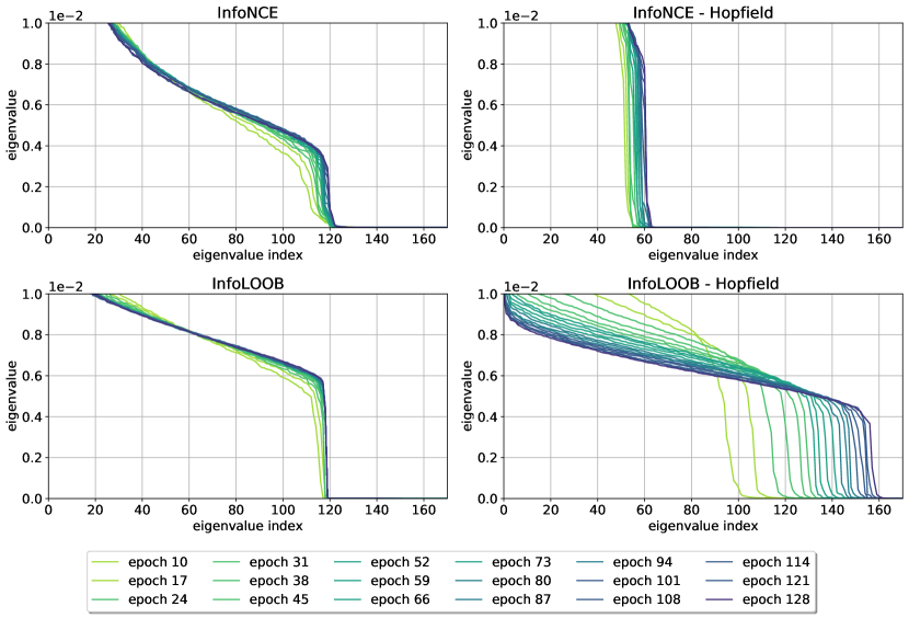
Additionally, we looked at the distribution of similarity scores (dot product) of matched pairs and unmatched pairs over the validation set of CC of embeddings from models trained for 128 epochs. In Figure A2, we contrast the distributions of similarity scores of matched pairs with the distributions of the similarity score for the 1,000 unmatched pairs that have the highest similarity score with the anchor. InfoNCE with Hopfield results in a moderate increase of the similarity scores of matched pairs, as well as in an increase of the similarity score of unmatched pairs. The latter is an undesired side effect of Hopfield networks as unmatched pairs get also more similar to one another. Compared to InfoNCE, InfoLOOB does not saturate. Therefore, it considerably increases the similarity between matched pairs and also reduces the average similarity of the top-1000 unmatched pairs. InfoLOOB attributes a cosine similarity of one to many pairs, which is not plausible for multi-modal pairs. Clearly, this is an overfitting problem of InfoLOOB. Noteworthy, an observed increase in alignment between epoch 31 and epoch 128 does not benefit the downstream performance. The combination of Hopfield and InfoLOOB increases the similarity score of matched pairs and simultaneously reduces the average similarity of unmatched pairs compared to InfoNCE without Hopfield (the CLIP setting).

Figure A2: Distribution of the cosine similarity of matched pairs and the cosine similarity of the 1,000 unmatched pairs that have the highest similarity score with the anchor.

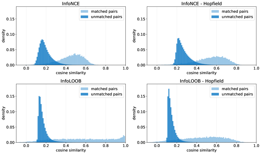
Figure A3 illustrates the overfitting problem of InfoLOOB. The distributions of unmatched pairs takes into account the ten unmatched pairs per anchor with the highest similarity score. In particular in the case of InfoLOOB without Hopfield, high similarity scores of the matched pairs correlate with high similarity scores of the top-10 unmatched pairs. In contrast, InfoLOOB with Hopfield does not suffer from this overfitting problem.

Figure A3: Distribution of the cosine similarity of matched pairs and the cosine similarity of the 10 unmatched pairs that have the highest similarity score with the anchor.

\begin{overpic}[width=143.09538pt,trim=0.0pt 0.0pt 0.0pt 0.0pt,clip]{figures/paper/zeroshot_plt_0.pdf} \put(18.0,55.0){ {Horse Riding}} \put(70.0,55.0){ {correct rank: 3/101}} \put(7.0,122.0){ {Dodge Caliber Wagon 2012}} \put(70.0,122.0){ {correct rank: 10/196}} \put(12.0,194.0){ {red circle with white}} \put(8.0,189.0){ {horizontal stripe no entry}} \put(70.0,189.0){ {correct rank: 4/43}} \put(24.0,257.0){ {azalea}} \put(70.0,257.0){ {correct rank: 1/102}} \put(22.0,324.0){ {Croatia}} \put(70.0,324.0){ {correct rank: 1/211}} \put(23.0,391.0){ {Osprey}} \put(70.0,391.0){ {correct rank: 1/500}} \put(23.0,458.0){ {mosque}} \put(70.0,458.0){ {correct rank: 1/1000}} \put(16.0,525.0){ {cottontail rabbit}} \put(70.0,525.0){ {correct rank: 1/1000}} \end{overpic}

(a)

\begin{overpic}[width=143.09538pt,trim=0.0pt 0.0pt 0.0pt 0.0pt,clip]{figures/paper/zeroshot_plt_1.pdf} \put(12.0,55.0){ {Handstand Walking}} \put(70.0,55.0){ {correct rank: 11/101}} \put(6.0,122.0){ {Chrysler Aspen SUV 2009}} \put(70.0,122.0){ {correct rank: 19/196}} \put(10.0,194.0){ {red and white circle red}} \put(4.0,189.0){ {truck and black car no passing}} \put(70.0,189.0){ {correct rank: 36/43}} \put(21.0,257.0){ {magnolia}} \put(70.0,257.0){ {correct rank: 1/102}} \put(23.0,324.0){ {Greece}} \put(70.0,324.0){ {correct rank: 1/211}} \put(14.0,391.0){ {Great Blue Heron}} \put(70.0,391.0){ {correct rank: 1/500}} \put(14.0,458.0){ {threshing machine}} \put(70.0,458.0){ {correct rank: 13/1000}} \put(16.0,525.0){ {longhorn beetle}} \put(70.0,525.0){ {correct rank: 1/1000}} \end{overpic}

(b)

\begin{overpic}[width=143.09538pt,trim=0.0pt 0.0pt 0.0pt 0.0pt,clip]{figures/paper/zeroshot_plt_2.pdf} \put(11.0,55.0){ {Field Hockey Penalty}} \put(70.0,55.0){ {correct rank: 1/101}} \put(4.0,122.0){ {Chevrolet Traverse SUV 2012}} \put(70.0,122.0){ {correct rank: 33/196}} \put(7.0,194.0){ {red and white triangle with}} \put(1.0,189.0){ {black curve approaching warning}} \put(70.0,189.0){ {correct rank: 11/43}} \put(24.0,257.0){ {rose}} \put(70.0,257.0){ {correct rank: 1/102}} \put(24.0,324.0){ {Spain}} \put(70.0,324.0){ {correct rank: 24/211}} \put(24.0,391.0){ {Brant}} \put(70.0,391.0){ {correct rank: 3/500}} \put(23.0,458.0){ {lipstick}} \put(70.0,458.0){ {correct rank: 7/1000}} \put(25.0,525.0){ {collie}} \put(70.0,525.0){ {correct rank: 2/1000}} \end{overpic}

(c)

Figure A4: Visualization of zero-shot classification of three examples from each dataset. The following datasets are used (top to bottom): ImageNet, ImageNet V2, Birdsnap, Country211, Flowers102, GTSRB, Stanford Cars and UCF101. The ground truth label is displayed above the picture. The bar plots show the softmax values of the top 5 classes.

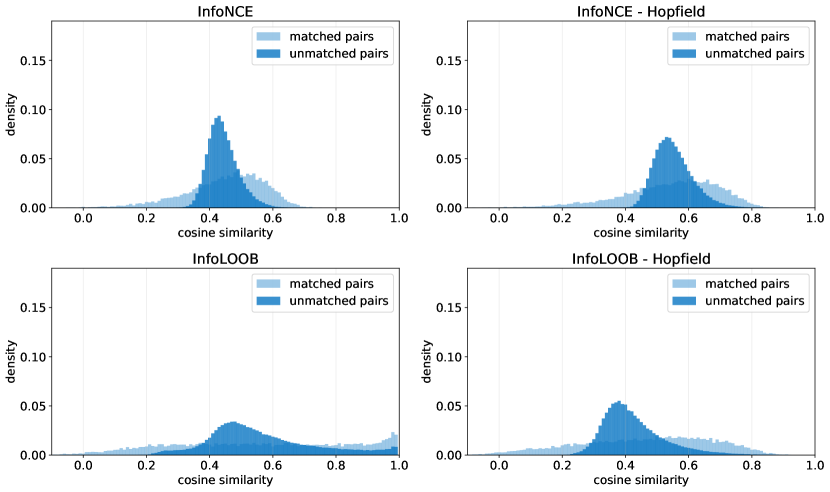
A.2.8 Training time and memory consumption

To elaborate on the time and memory consumption of CLOOB, Table A9 compares the experiments done in Section 5.1. The memory consumption of CLOOB is the same as CLIP since only embeddings from the mini-batch are used both in the objective and in the Hopfield memories. The time consumption is approximately $5\%$ higher, which is because of the retrieval of the modern Hopfield networks. The added complexity of modern Hopfield networks is $\mathcal{O}(N)$ per sample, where $N$ denotes the batch size.

Table A9: Memory and time consumption of CLIP and CLOOB when trained for 31 epochs on CC.

Model	Batch size (per GPU)	Memory (per GPU)	GPU hours	ImageNet zero-shot
CLIP	128	13.7GB	141	20.3
CLOOB	128	13.7GB	148	24.0

A.3 Review of Modern Hopfield Networks

We briefly review continuous modern Hopfield networks that are used for deep learning architectures. They are continuous and differentiable, therefore they a work with gradient descent in deep architectures. They retrieve with one update only, therefore they can be activated like other deep learning layers. They have exponential storage capacity, therefore they can tackle large problems. Hopfield networks are energy-based, binary associative memories, which popularized artificial neural networks in the 1980s (Hopfield, 1982, 1984). Associative memory networks have been designed to store and retrieve samples. Their storage capacity can be considerably increased by polynomial terms in the energy function (Chen et al., 1986; Psaltis & Cheol, 1986; Baldi & Venkatesh, 1987; Gardner, 1987; Abbott & Arian, 1987; Horn & Usher, 1988; Caputo & Niemann, 2002; Krotov & Hopfield, 2016). In contrast to these binary memory networks, we use continuous associative memory networks with very high storage capacity. These modern Hopfield networks for deep learning architectures have an energy function with continuous states and can retrieve samples with only one update (Ramsauer et al., 2021). Modern Hopfield Networks have been successfully applied to immune repertoire classification (Widrich et al., 2020) and chemical reaction prediction (Seidl et al., 2021).

We assume a set of patterns $\{\bm{u}_{1},\ldots,\bm{u}_{N}\}\subset\mathbb{R}^{d}$ that are stacked as columns to the matrix $\bm{U}=\left(\bm{u}_{1},\ldots,\bm{u}_{N}\right)$ and a state pattern (query) $\bm{\xi}\in\mathbb{R}^{d}$ that represents the current state. The largest norm of a stored pattern is $M=\max_{i}{{\left\|\bm{u}_{i}\right\|}}$. Continuous modern Hopfield networks with state $\bm{\xi}$ have the energy

$$\mathrm{E}\ =\ -\ \beta^{-1}\ \log\left(\sum_{i=1}^{N}\exp(\beta\bm{u}_{i}^{T}\bm{\xi})\right)\ +\ \beta^{-1}\log N\ +\ \frac{1}{2}\ \bm{\xi}^{T}\bm{\xi}\ +\ \frac{1}{2}\ M^{2}\ .$$ (A178)

For energy $\mathrm{E}$ and state $\bm{\xi}$, the update rule

$$\bm{\xi}^{\mathrm{new}}\ =\ f(\bm{\xi};\bm{U},\beta)\ =\ \bm{U}\ \bm{p}\ =\ \bm{U}\ \mathrm{softmax}(\beta\bm{U}^{T}\bm{\xi})$$ (A179)

has been proven to converge globally to stationary points of the energy $\mathrm{E}$, which are almost always local minima (Ramsauer et al., 2021). The update rule Eq. (A179) is also the formula of the well-known transformer attention mechanism (Ramsauer et al., 2021), therefore Hopfield retrieval and transformer attention coincide.

The separation $\Delta_{i}$ of a pattern $\bm{u}_{i}$ is defined as its minimal dot product difference to any of the other patterns: $\Delta_{i}=\min_{j,j\not=i}\left(\bm{u}_{i}^{T}\bm{u}_{i}-\bm{u}_{i}^{T}\bm{u}_{j}\right)$. A pattern is well-separated from the data if $\Delta_{i}\geq\frac{2}{\beta N}+\frac{1}{\beta}\log\left(2(N-1)N\beta M^{2}\right)$. If the patterns $\bm{u}_{i}$ are well separated, the iterate Eq. (A179) converges to a fixed point close to a stored pattern. If some patterns are similar to one another and, therefore, not well separated, the update rule Eq. (A179) converges to a fixed point close to the mean of the similar patterns. This fixed point is a metastable state of the energy function and averages over similar patterns.

The next theorem states that the update rule Eq. (A179) typically converges after one update if the patterns are well separated. Furthermore, it states that the retrieval error is exponentially small in the separation $\Delta_{i}$.

Theorem A4 (Modern Hopfield Networks: Retrieval with One Update).

With query $\bm{\xi}$, after one update the distance of the new point $f(\bm{\xi})$ to the fixed point $\bm{u}_{i}^{*}$ is exponentially small in the separation $\Delta_{i}$. The precise bounds using the Jacobian $\mathrm{J}=\frac{\partial f(\bm{\xi})}{\partial\bm{\xi}}$ and its value $\mathrm{J}^{m}$ in the mean value theorem are:

$${{\left\|f(\bm{\xi})\ -\ \bm{u}_{i}^{*}\right\|}}\ \leqslant\ {{\left\|\mathrm{J}^{m}\right\|}}_{2}\ {{\left\|\bm{\xi}\ -\ \bm{u}_{i}^{*}\right\|}}\ ,$$ (A180)

$${{\left\|\mathrm{J}^{m}\right\|}}_{2}\ \leqslant\ 2\ \beta\ N\ M^{2}\ (N-1)\exp(-\ \beta\ (\Delta_{i}\ -\ 2\ \max\{{{\left\|\bm{\xi}\ -\ \bm{u}_{i}\right\|}},{{\left\|\bm{u}_{i}^{*}\ -\ \bm{u}_{i}\right\|}}\}\ M))\ .$$ (A181)

For given $\epsilon$ and sufficient large $\Delta_{i}$, we have ${{\left\|f(\bm{\xi})\ -\ \bm{u}_{i}^{*}\right\|}}<\epsilon$, that is, retrieval with one update. The retrieval error ${{\left\|f(\bm{\xi})\ -\ \bm{u}_{i}\right\|}}$ of pattern $\bm{u}_{i}$ is bounded by

$${{\left\|f(\bm{\xi})\ -\ \bm{u}_{i}\right\|}}\ \leqslant\ 2\ (N-1)\ \exp(-\ \beta\ (\Delta_{i}\ -\ 2\ \max\{{{\left\|\bm{\xi}\ -\ \bm{u}_{i}\right\|}},{{\left\|\bm{u}_{i}^{*}\ -\ \bm{u}_{i}\right\|}}\}\ M))\ M\ .$$ (A182)

For a proof see (Ramsauer et al., 2021).

The main requirement of modern Hopfield networks to be suited for contrastive learning is that they can store and retrieve enough embeddings if the batch size is large. We want to store a potentially large set of embeddings. We first define what we mean by storing and retrieving patterns from a modern Hopfield network.

Definition A1 (Pattern Stored and Retrieved).

We assume that around every pattern $\bm{u}_{i}$ a sphere $\mathrm{S}_{i}$ is given. We say $\bm{u}_{i}$ is stored if there is a single fixed point $\bm{u}_{i}^{*}\in\mathrm{S}_{i}$ to which all points $\bm{\xi}\in\mathrm{S}_{i}$ converge, and $\mathrm{S}_{i}\cap\mathrm{S}_{j}=\emptyset$ for $i\not=j$. We say $\bm{u}_{i}$ is retrieved for a given $\epsilon$ if iteration (update rule) Eq. (A179) gives a point $\tilde{\bm{x}}_{i}$ that is at least $\epsilon$-close to the single fixed point $\bm{u}_{i}^{*}\in\mathrm{S}_{i}$. The retrieval error is ${{\left\|\tilde{\bm{x}}_{i}-\bm{u}_{i}\right\|}}$.

As with classical Hopfield networks, we consider patterns on the sphere, i.e. patterns with a fixed norm. For randomly chosen patterns, the number of patterns that can be stored is exponential in the dimension $d$ of the space of the patterns ($\bm{u}_{i}\in\mathbb{R}^{d}$).

Theorem A5 (Modern Hopfield Networks: Exponential Storage Capacity).

We assume a failure probability $0<p\leqslant 1$ and randomly chosen patterns on the sphere with radius $M:=K\sqrt{d-1}$. We define $a:=\frac{2}{d-1}(1+\ln(2\beta K^{2}p(d-1)))$, $b:=\frac{2K^{2}\beta}{5}$, and $c:=\frac{b}{W_{0}(\exp(a+\ln(b))}$, where $W_{0}$ is the upper branch of the Lambert $W$ function (Olver et al., 2010, (4.13) ) , and ensure $c\geq\left(\frac{2}{\sqrt{p}}\right)^{\frac{4}{d-1}}$. Then with probability $1-p$, the number of random patterns that can be stored is

$$N\ \geq\ \sqrt{p}\ c^{\frac{d-1}{4}}\ .$$ (A183)

Therefore it is proven for $c\geq 3.1546$ with $\beta=1$, $K=3$, $d=20$ and $p=0.001$ ($a+\ln(b)>1.27$) and proven for $c\geq 1.3718$ with $\beta=1$, $K=1$, $d=75$, and $p=0.001$ ($a+\ln(b)<-0.94$).

For a proof see (Ramsauer et al., 2021).

This theorem justifies to use continuous modern Hopfield networks for using retrieved embeddings instead of the original embeddings for large batch sizes. Even for hundreds of thousands of embeddings, the continuous modern Hopfield network is able to retrieve the embeddings if the dimension of the embeddings is large enough.

A.4 Further Related Work

With the advent of large corpora of unlabeled data in vision and language, self-supervised learning via contrastive learning has become highly successful. Some contrastive learning objectives, such as those of BYOL (Grill et al., 2020) and SimSiam (Chen & He, 2021), do not require negative samples. However, the most popular objective for contrastive learning is InfoNCE (van den Oord et al., 2018), in which for an anchor sample, a positive sample is contrasted with negative samples.

The idea to use objectives with negative samples is well known in deep learning (Gutmann & Hyvärinen, 2010; Chen et al., 2017; Mikolov et al., 2013). For contrastive learning, the most successful objective is InfoNCE, which has been introduced as Contrastive Predictive Coding (CPC) (van den Oord et al., 2018). InfoNCE has been applied to transfer learning (Hénaff et al., 2019), to natural language response suggestion (Henderson et al., 2017), to learning sentence representations from unlabelled data (Logeswaran & Lee, 2018), and to unsupervised feature learning by maximizing distinctions between instances (Wu et al., 2018). InfoNCE has been used for learning visual representations in Pretext-Invariant Representation Learning (PIRL) (Misra & vanDerMaaten, 2020), in Momentum Contrast (MoCo) (He et al., 2020), and in SimCLR (Chen et al., 2020). SimCLR became well known as is was highly effective for transfer learning. Zero-shot transfer learning (Lampert et al., 2009) is one of the most ambitious goals in vision, since it would improve various real-world downstream applications. Current models in natural language processing and vision perform very well on standard benchmarks, but they fail at new data, new applications, deployments in the wild, and stress tests (D’Amour et al., 2020; Recht et al., 2019; Taori et al., 2020; Lapuschkin et al., 2019; Geirhos et al., 2020). A model with high zero-shot transfer learning performance will not fail on such data, therefore will be trusted by practitioners.

Multiple works have proposed improvements to InfoNCE. Joint Contrastive Learning (JCL) studies the effect of sampling multiple positives for each anchor. (Cai et al., 2020). Sampling negatives around each positive leads to higher bias but lower variance than InfoNCE (Wu et al., 2021). InfoNCE has been generalized to C-InfoNCE and WeaC-InfoNCE, which are conditional contrastive learning approaches to remove undesirable information in self-supervised representations (Tsai et al., 2021). ProtoNCE is a generalized version of the InfoNCE, which pushes representations to be closer to their assigned prototypes (Li et al., 2021). ProtoNCE combines contrastive learning with clustering. SimCSE employs InfoNCE for contrastive learning to learn sentence embeddings (Gao et al., 2021). InfoNCE has been extended to video representation learning (Han et al., 2020).

CLOOB uses InfoLOOB, which is an upper bound on the mutual information. An alternative upper bound on the mutual information would be Contrastive Log-ratio Upper Bound (CLUB), which was used for minimizing the mutual information (Cheng et al., 2020). So far CLUB was only used for minimizing the mutual information, except for the analysis in (Wang & Liu, 2021). In our experiments, maximizing CLUB failed as confirmed in (Wang & Liu, 2021). The reason is that the embedding distribution is not uniform as required for successful contrastive learning (Wang & Isola, 2020; Wang & Liu, 2021).

Many follow up works have been based on the CLIP model. The CLIP model is used in Vision-and-Language tasks (Shen et al., 2021). The CLIP model guided generative models via an additional training objective (Bau et al., 2021; Galatolo et al., 2021; Frans et al., 2021) and improved clustering of latent representations (Pakhomov et al., 2021). It is used in studies of out of distribution performance (Devillers et al., 2021; Milbich et al., 2021; Miller et al., 2021), of fine-tuning robustness (Wortsman et al., 2021), of zero-shot prompts (Zhou et al., 2021) and of adversarial attacks to uncurated datasets (Carlini & Terzis, 2021). It stirred discussions about more holistic evaluation schemes in computer vision (Agarwal et al., 2021). Multiple methods utilize the CLIP model in a straightforward way to perform text-to-video retrieval (Fang et al., 2021; Luo et al., 2021; Narasimhan et al., 2021).

References

• Abbott & Arian (1987) Abbott, L. F. and Arian, Y. Storage capacity of generalized networks. Physical Review A, 36:5091–5094, 1987. doi: 10.1103/PhysRevA.36.5091.
• Agarwal et al. (2021) Agarwal, S., Krueger, G., Clark, J., Radford, A., Kim, J. W., and Brundage, M. Evaluating CLIP: Towards characterization of broader capabilities and downstream implications. ArXiv, 2108.02818, 2021.
• Ajne (1968) Ajne, B. A simple test for uniformity of a circular distribution. Biometrika, 55(2):343–354, 1968. doi: 10.1093/biomet/55.2.343.
• Amari (1972) Amari, S.-I. Learning patterns and pattern sequences by self-organizing nets of threshold elements. IEEE Transactions on Computers, C-21(11):1197–1206, 1972. doi: 10.1109/T-C.1972.223477.
• Arbel et al. (2019) Arbel, J., Marchal, O., and Nguyen, H. D. On strict sub-Gaussianity, optimal proxy variance and symmetry for bounded random variables. ArXiv, 1901.09188, 2019.
• Baldi & Venkatesh (1987) Baldi, P. and Venkatesh, S. S. Number of stable points for spin-glasses and neural networks of higher orders. Physical Review Letters, 58:913–916, 1987. doi: 10.1103/PhysRevLett.58.913.
• Bau et al. (2021) Bau, D., Andonian, A., Cui, A., Park, Y., Jahanian, A., Oliva, A., and Torralba, A. Paint by word. ArXiv, 2103.10951, 2021.
• Belghazi et al. (2018) Belghazi, M. I., Baratin, A., Rajeswar, S., Ozair, S., Bengio, Y., Courville, A., and Hjelm, R. D. Mutual information neural estimation. In Dy, J. and Krause, A. (eds.), Proceedings of International Conference on Machine Learning (ICML), pp.  531–540, 2018.
• Berg et al. (2014) Berg, T., Liu, J., Lee, S. W., Alexander, M. L., Jacobs, D. W., and Belhumeur, P. N. Birdsnap: Large-scale fine-grained visual categorization of birds. In Proceedings of the Conference on Computer Vision and Pattern Recognition (CVPR), pp.  2019–2026, 2014. doi: 10.1109/CVPR.2014.259.
• Biewald (2020) Biewald, L. Experiment tracking with weights and biases, 2020. URL https://www.wandb.com/. Software available from wandb.com.
• Bommasani et al. (2021) Bommasani, R. et al. On the opportunities and risks of foundation models. ArXiv, 2108.07258, 2021.
• Bonner & Epstein (2021) Bonner, M. F. and Epstein, R. A. Object representations in the human brain reflect the co-occurrence statistics of vision and language. Nature Communications, 12(4081), 2021. doi: 10.1038/s41467-021-24368-2.
• Bossard et al. (2014) Bossard, L., Guillaumin, M., and Van Gool, L. Food-101 – mining discriminative components with random forests. In European Conference on Computer Vision, 2014.
• Cai et al. (2020) Cai, Q., Wang, Y., Pan, Y., Yao, T., and Mei, T. Joint contrastive learning with infinite possibilities. In Larochelle, H., Ranzato, M., Hadsell, R., Balcan, M. F., and Lin, H. (eds.), Advances in Neural Information Processing Systems (NeurIPS), pp.  12638–12648, 2020.
• Caputo & Niemann (2002) Caputo, B. and Niemann, H. Storage capacity of kernel associative memories. In Proceedings of the International Conference on Artificial Neural Networks (ICANN), pp.  51–56, Berlin, Heidelberg, 2002. Springer-Verlag.
• Carlini & Terzis (2021) Carlini, N. and Terzis, A. Poisoning and backdooring contrastive learning. ArXiv, 2106.09667, 2021.
• Chen et al. (1986) Chen, H. H., Lee, Y. C., Sun, G. Z., Lee, H. Y., Maxwell, T., and Giles, C. L. High order correlation model for associative memory. AIP Conference Proceedings, 151(1):86–99, 1986. doi: 10.1063/1.36224.
• Chen et al. (2021) Chen, J., Gan, Z., Li, X., Guo, Q., Chen, L., Gao, S., Chung, T., Xu, Y., Zeng, B., Lu, W., Li, F., Carin, L., and Tao, C. Simpler, faster, stronger: Breaking the log-K curse on contrastive learners with FlatNCE. arXiv, 2107.01152, 2021.
• Chen et al. (2017) Chen, T., Sun, Y., Shi, Y., and Hong, L. On sampling strategies for neural network-based collaborative filtering. In Proceedings of the International Conference on Knowledge Discovery and Data Mining, pp.  767–776, New York, NY, USA, 2017. Association for Computing Machinery. doi: 10.1145/3097983.3098202.
• Chen et al. (2020) Chen, T., Kornblith, S., Norouzi, M., and Hinton, G. A simple framework for contrastive learning of visual representations. In Daumé, H. and Singh, A. (eds.), Proceedings of the International Conference on Machine Learning (ICML), pp.  1597–1607, 2020.
• Chen & He (2021) Chen, X. and He, K. Exploring simple siamese representation learning. In Proceedings of the Conference on Computer Vision and Pattern Recognition (CVPR), pp.  15750–15758, 2021.
• Cheng et al. (2017) Cheng, G., Han, J., and Lu, X. Remote sensing image scene classification: Benchmark and state of the art. Proceedings of the IEEE, 105(10):1865–1883, Oct 2017. ISSN 1558-2256. doi: 10.1109/jproc.2017.2675998.
• Cheng et al. (2020) Cheng, P., Hao, W., Dai, S., Liu, J., Gan, Z., and Carin, L. CLUB: A contrastive log-ratio upper bound of mutual information. In Daume, H. and Singh, A. (eds.), International Conference on Machine Learning (ICLR), pp.  1779–1788, 2020.
• Cimpoi et al. (2014) Cimpoi, M., Maji, S., Kokkinos, I., Mohamed, S., , and Vedaldi, A. Describing textures in the wild. In Proceedings of the IEEE Conf. on Computer Vision and Pattern Recognition (CVPR), 2014.
• Coates et al. (2011) Coates, A., Ng, A., and Lee, H. An Analysis of Single Layer Networks in Unsupervised Feature Learning. In AISTATS, 2011.
• D’Amour et al. (2020) D’Amour, A. et al. Underspecification presents challenges for credibility in modern machine learning. ArXiv, 2011.03395, 2020.
• Deng et al. (2009) Deng, J., Dong, W., Socher, R., Li, L.-J., Li, K., and Fei-Fei, L. Imagenet: A large-scale hierarchical image database. In Proceedings of the Conference on Computer Vision and Pattern Recognition (CVPR), pp.  248–255. Ieee, 2009.
• Devillers et al. (2021) Devillers, B., Bielawski, R., Choski, B., and VanRullen, R. Does language help generalization in vision models? ArXiv, 2104.08313, 2021.
• Devlin et al. (2018) Devlin, J., Chang, M.-W., Lee, K., and Toutanova, K. BERT: Pre-training of deep bidirectional transformers for language understanding. ArXiv, 2018.
• Devlin et al. (2019) Devlin, J., Chang, M.-W., Lee, K., and Toutanova, K. BERT: Pre-training of deep bidirectional transformers for language understanding. In Proceedings of the Conference of the North American Chapter of the Association for Computational Linguistics: Human Language Technologies, pp.  4171–4186. Association for Computational Linguistics, 2019. doi: 10.18653/v1/N19-1423.
• Fang et al. (2021) Fang, H., Xiong, P., Xu, L., and Chen, Y. CLIP2Video: Mastering video-text retrieval via image CLIP. ArXiv, 2106.11097, 2021.
• Fei-Fei et al. (2004) Fei-Fei, L., Fergus, R., and Perona, P. Learning generative visual models from few training examples: An incremental bayesian approach tested on 101 object categories. Computer Vision and Pattern Recognition Workshop, 2004.
• Frans et al. (2021) Frans, K., Soros, L. B., and Witkowski, O. CLIPDraw: Exploring text-to-drawing synthesis through language-image encoders. ArXiv, 2106.14843, 2021.
• Galatolo et al. (2021) Galatolo, F. A., Cimino, M. G. C. A., and Vaglini, G. Generating images from caption and vice versa via CLIP-guided generative latent space search. ArXiv, 2102.01645, 2021.
• Gao & Pavel (2017) Gao, B. and Pavel, L. On the properties of the softmax function with application in game theory and reinforcement learning. ArXiv, 2017.
• Gao et al. (2021) Gao, T., Yao, X., and Chen, D. SimCSE: Simple contrastive learning of sentence embeddings. ArXiv, 2104.08821, 2021.
• Gardner (1987) Gardner, E. Multiconnected neural network models. Journal of Physics A, 20(11):3453–3464, 1987. doi: 10.1088/0305-4470/20/11/046.
• Geirhos et al. (2020) Geirhos, R., Jacobsen, J.-H., Michaelis, C., Zemel, R. S., Brendel, W., Bethge, M., and Wichmann, F. A. Shortcut learning in deep neural networks. ArXiv, 2004.07780, 2020.
• Goodfellow et al. (2013) Goodfellow, I. J., Erhan, D., Carrier, P. L., Courville, A., Mirza, M., Hamner, B., Cukierski, W., Tang, Y., Thaler, D., Lee, D.-H., Zhou, Y., Ramaiah, C., Feng, F., Li, R., Wang, X., Athanasakis, D., Shawe-Taylor, J., Milakov, M., Park, J., Ionescu, R., Popescu, M., Grozea, C., Bergstra, J., Xie, J., Romaszko, L., Xu, B., Chuang, Z., and Bengio, Y. Challenges in representation learning: A report on three machine learning contests, 2013.
• Grill et al. (2020) Grill, J.-B., Strub, F., Altché, F., Tallec, C., Richemond, P. H., Buchatskaya, E., Doersch, C., Pires, B. Á., Guo, Z. D., Azar, M. G., Piot, B., Kavukcuoglu, K., Munos, R., and Valko, M. Bootstrap your own latent - a new approach to self-supervised learning. In Larochelle, H., Ranzato, M., Hadsell, R., Balcan, M. F., and Lin, H. (eds.), Advances in Neural Information Processing Systems (NeurIPS), pp.  21271–21284, 2020.
• Gutmann & Hyvärinen (2010) Gutmann, M. and Hyvärinen, A. Noise-contrastive estimation: A new estimation principle for unnormalized statistical models. In Teh, Y. W. and Titterington, M. (eds.), International Conference on Artificial Intelligence and Statistics, pp.  297–304, 2010.
• Han et al. (2020) Han, T., Xie, W., and Zisserman, A. Self-supervised co-training for video representation learning. In Larochelle, H., Ranzato, M., Hadsell, R., Balcan, M. F., and Lin, H. (eds.), Advances in Neural Information Processing Systems (NeurIPS), pp.  5679–5690, 2020.
• He et al. (2016) He, K., Zhang, X., Ren, S., and Sun, J. Deep residual learning for image recognition. In Proceedings of the IEEE Conference on Computer Vision and Pattern Recognition (CVPR), 2016.
• He et al. (2020) He, K., Fan, H., Wu, Y., Xie, S., and Girshick, R. B. Momentum contrast for unsupervised visual representation learning. In Proceedings of the Conference on Computer Vision and Pattern Recognition (CVPR), 2020.
• Helber et al. (2018) Helber, P., Bischke, B., Dengel, A., and Borth, D. Introducing eurosat: A novel dataset and deep learning benchmark for land use and land cover classification. In IGARSS 2018-2018 IEEE International Geoscience and Remote Sensing Symposium, pp.  204–207. IEEE, 2018.
• Helber et al. (2019) Helber, P., Bischke, B., Dengel, A., and Borth, D. Eurosat: A novel dataset and deep learning benchmark for land use and land cover classification. IEEE Journal of Selected Topics in Applied Earth Observations and Remote Sensing, 2019.
• Hénaff et al. (2019) Hénaff, O. J., Srinivas, A., DeFauw, J., Razavi, A., Doersch, C., Eslami, S. M. A., and vanDenOord, A. Data-efficient image recognition with contrastive predictive coding. ArXiv, 1905.09272, 2019.
• Henderson et al. (2017) Henderson, M. L., Al-Rfou, R., Strope, B., Sung, Y.-H., Lukács, L., Guo, R., Kumar, S., Miklos, B., and Kurzweil, R. Efficient natural language response suggestion for smart reply. ArXiv, 1705.00652, 2017.
• Hopfield (1982) Hopfield, J. J. Neural networks and physical systems with emergent collective computational abilities. In Proceedings of the National Academy of Sciences, volume 79, pp.  2554–2558, 1982.
• Hopfield (1984) Hopfield, J. J. Neurons with graded response have collective computational properties like those of two-state neurons. In Proceedings of the National Academy of Sciences, volume 81, pp.  3088–3092. National Academy of Sciences, 1984. doi: 10.1073/pnas.81.10.3088.
• Horn & Usher (1988) Horn, D. and Usher, M. Capacities of multiconnected memory models. Journal of Physics France, 49(3):389–395, 1988. doi: 10.1051/jphys:01988004903038900.
• Ilharco et al. (2021) Ilharco, G., Wortsman, M., Carlini, N., Taori, R., Dave, A., Shankar, V., Namkoong, H., Miller, J., Hajishirzi, H., Farhadi, A., and Schmidt, L. OpenCLIP, 2021.
• Jing et al. (2022) Jing, L., Vincent, P., LeCun, Y., and Tian, Y. Understanding dimensional collapse in contrastive self-supervised learning. In International Conference on Learning Representations (ICLR). OpenReview, 2022.
• Kingma et al. (2014) Kingma, D. P., Mohamed, S., Rezende, D. J., and Welling, M. Semi-supervised learning with deep generative models. In Ghahramani, Z., Welling, M., Cortes, C., Lawrence, N. D., and Weinberger, K. Q. (eds.), Advances in Neural Information Processing Systems (NeurIPS), pp.  3581–3589. 2014.
• Krause et al. (2013) Krause, J., Stark, M., Deng, J., and Fei-Fei, L. 3D object representations for fine-grained categorization. In International IEEE Workshop on 3D Representation and Recognition (3dRR-13), 2013.
• Krizhevsky (2009) Krizhevsky, A. Learning multiple layers of features from tiny images. Technical report, 2009.
• Krotov & Hopfield (2016) Krotov, D. and Hopfield, J. J. Dense associative memory for pattern recognition. In Lee, D. D., Sugiyama, M., Luxburg, U. V., Guyon, I., and Garnett, R. (eds.), Advances in Neural Information Processing Systems (NeurIPS), pp.  1172–1180, 2016.
• Lampert et al. (2009) Lampert, C. H., Nickisch, H., and Harmeling, S. Learning to detect unseen object classes by between-class attribute transfer. In Proceedings of the Conference on Computer Vision and Pattern Recognition (CVPR), pp.  951–958, 2009.
• Lapuschkin et al. (2019) Lapuschkin, S., Wäldchen, S., Binder, A., Montavon, G., Samek, W., and Müller, K.-R. Unmasking Clever Hans predictors and assessing what machines really learn. Nature Communications, 10, 2019. doi: 10.1038/s41467-019-08987-4.
• Li et al. (2021) Li, J., Zhou, P., Xiong, C., Socher, R., and Hoi, S. C. H. Prototypical contrastive learning of unsupervised representations. In International Conference on Learning Representations (ICLR). OpenReview, 2021.
• Logeswaran & Lee (2018) Logeswaran, L. and Lee, H. An efficient framework for learning sentence representations. In International Conference on Learning Representations (ICLR). OpenReview, 2018.
• Loshchilov & Hutter (2017) Loshchilov, I. and Hutter, F. SGDR: Stochastic gradient descent with warm restarts. In International Conference on Learning Representations (ICLR). OpenReview, 2017.
• Loshchilov & Hutter (2019) Loshchilov, I. and Hutter, F. Decoupled weight decay regularization. In International Conference on Learning Representations (ICLR). OpenReview, 2019.
• Luo et al. (2021) Luo, H., Ji, L., Zhong, M., Chen, Y., Lei, W., Duan, N., and Li, T. CLIP4Clip: An empirical study of CLIP for end to end video clip retrieval. ArXiv, 2104.08860, 2021.
• Maji et al. (2013) Maji, S., Kannala, J., Rahtu, E., Blaschko, M., and Vedaldi, A. Fine-grained visual classification of aircraft. Technical report, 2013.
• McAllester & Stratos (2018) McAllester, D. and Stratos, K. Formal limitations on the measurement of mutual information. ArXiv, 1811.04251, 2018.
• McAllester & Stratos (2020) McAllester, D. and Stratos, K. Formal limitations on the measurement of mutual information. In Chiappa, S. and Calandra, R. (eds.), Proceedings of the International Conference on Artificial Intelligence and Statistics, pp. 875–884, 26–28 Aug 2020.
• Mikolov et al. (2013) Mikolov, T., Sutskever, I., Chen, K., Corrado, G. S., and Dean, J. Distributed representations of words and phrases and their compositionality. In Burges, C. J. C., Bottou, L., Welling, M., Ghahramani, Z., and Weinberger, K. Q. (eds.), Advances in Neural Information Processing Systems (NeurIPS), pp.  3111–3119, 2013.
• Milbich et al. (2021) Milbich, T., Roth, K., Sinha, S., Schmidt, L., Ghassemi, M., and Ommer, B. Characterizing generalization under out-of-distribution shifts in deep metric learning. ArXiv, 2107.09562, 2021.
• Miller et al. (2021) Miller, J., Taori, R., Raghunathan, A., Sagawa, S., Koh, P. W., Shankar, V., Liang, P., Carmon, Y., and Schmidt, L. Accuracy on the line: On the strong correlation between out-of-distribution and in-distribution generalization. ArXiv, 2107.04649, 2021.
• Misra & vanDerMaaten (2020) Misra, I. and vanDerMaaten, L. Self-supervised learning of pretext-invariant representations. In Proceedings of the Conference on Computer Vision and Pattern Recognition (CVPR), 2020.
• Narasimhan et al. (2021) Narasimhan, M., Rohrbach, A., and Darrell, T. CLIP-It! Language-guided video summarization. ArXiv, 2107.00650, 2021.
• Nguyen et al. (2010) Nguyen, X., Wainwright, M. J., and Jordan, M. Estimating divergence functionals and the likelihood ratio by penalized convex risk minimization. IEEE Transactions on Information Theory, 56(11):5847–5861, 2010. doi: 10.1109/tit.2010.2068870.
• Nilsback & Zisserman (2008) Nilsback, M.-E. and Zisserman, A. Automated flower classification over a large number of classes. In Proceedings of the Indian Conference on Computer Vision, Graphics and Image Processing, pp.  722–729. IEEE Computer Society, 2008. doi: 10.1109/ICVGIP.2008.47.
• Olver et al. (2010) Olver, F. W. J., Lozier, D. W., Boisvert, R. F., and Clark, C. W. NIST handbook of mathematical functions. Cambridge University Press, 1 pap/cdr edition, 2010. ISBN 9780521192255.
• Paischer et al. (2022) Paischer, F., Adler, T., Patil, V., Bitto-Nemling, A., Holzleitner, M., Lehner, S., Eghbal-Zadeh, H., and Hochreiter, S. History compression via language models in reinforcement learning. In Chaudhuri, K., Jegelka, S., Song, L., Szepesvari, C., Niu, G., and Sabato, S. (eds.), Proceedings of the 39th International Conference on Machine Learning, pp.  17156–17185, 2022.
• Pakhomov et al. (2021) Pakhomov, D., Hira, S., Wagle, N., Green, K. E., and Navab, N. Segmentation in style: Unsupervised semantic image segmentation with stylegan and CLIP. ArXiv, 2107.12518, 2021.
• Parkhi et al. (2012) Parkhi, O. M., Vedaldi, A., Zisserman, A., and Jawahar, C. V. Cats and dogs. In IEEE Conference on Computer Vision and Pattern Recognition, 2012.
• Paszke et al. (2017) Paszke, A., Gross, S., Chintala, S., Chanan, G., Yang, E., DeVito, Z., Lin, Z., Desmaison, A., Antiga, L., and Lerer, A. Automatic differentiation in pytorch. 2017.
• Pearl (1988) Pearl, J. Embracing causality in default reasoning. Artificial Intelligence, 35(2):259–271, 1988.
• Poole et al. (2019) Poole, B., Ozair, S., vanDenOord, A., Alemi, A. A., and Tucker, G. On variational bounds of mutual information. In Chaudhuri, K. and Salakhutdinov, R. (eds.), Proceedings of the International Conference on Machine Learning (ICML), pp.  5171–5180, 2019.
• Potter (2012) Potter, M. Conceptual short term memory in perception and thought. Frontiers in Psychology, 3:113, 2012. doi: 10.3389/fpsyg.2012.00113.
• Prentice (1978) Prentice, M. J. On invariant tests of uniformity for directions and orientations. The Annals of Statistics, 6(1):169–176, 1978. doi: 10.1214/aos/1176344075.
• Psaltis & Cheol (1986) Psaltis, D. and Cheol, H. P. Nonlinear discriminant functions and associative memories. AIP Conference Proceedings, 151(1):370–375, 1986. doi: 10.1063/1.36241.
• Radford et al. (2021) Radford, A., Kim, J. W., Hallacy, C., Ramesh, A., Goh, G., Agarwal, S., Sastry, G., Askell, A., Mishkin, P., Clark, J., Krueger, G., and Sutskever, I. Learning transferable visual models from natural language supervision. In Proceedings of the International Conference on Machine Learning (ICML), 2021.
• Ramsauer et al. (2021) Ramsauer, H., Schäfl, B., Lehner, J., Seidl, P., Widrich, M., Gruber, L., Holzleitner, M., Pavlović, M., Sandve, G. K., Greiff, V., Kreil, D., Kopp, M., Klambauer, G., Brandstetter, J., and Hochreiter, S. Hopfield networks is all you need. In International Conference on Learning Representations (ICLR). OpenReview, 2021.
• Recht et al. (2019) Recht, B., Roelofs, R., Schmidt, L., and Shankar, V. Do ImageNet classifiers generalize to ImageNet? In Chaudhuri, K. and Salakhutdinov, R. (eds.), Proceedings of the International Conference on Machine Learning (ICML), pp.  5389–5400, 2019.
• Seidl et al. (2021) Seidl, P., Renz, P., Dyubankova, N., Neves, P., Verhoeven, J., Wegner, J. K., Hochreiter, S., and Klambauer, G. Modern Hopfield networks for few- and zero-shot reaction prediction. ArXiv, 2104.03279, 2021.
• Seidl et al. (2022) Seidl, P., Renz, P., Dyubankova, N., Neves, P., Verhoeven, J., Wegner, J. K., Segler, M., Hochreiter, S., and Klambauer, G. Improving few-and zero-shot reaction template prediction using modern Hopfield networks. Journal of Chemical Information and Modeling, 2022.
• Sharma et al. (2018) Sharma, P., Ding, N., Goodman, S., and Soricut, R. Conceptual captions: A cleaned, hypernymed, image alt-text dataset for automatic image captioning. In Proceedings of the Association for Computational Linguistics (ACL), 2018.
• Shen et al. (2021) Shen, S., Li, L. H., Tan, H., Bansal, M., Rohrbach, A., Chang, K.-W., Yao, Z., and Keutzer, K. How much can CLIP benefit vision-and-language tasks? ArXiv, 2107.06383, 2021.
• Soomro et al. (2012) Soomro, K., Zamir, A. R., and Shah, M. A dataset of 101 human action classes from videos in the wild. Center for Research in Computer Vision, 2(11), 2012.
• Stallkamp et al. (2011) Stallkamp, J., Schlipsing, M., Salmen, J., and Igel, C. The German traffic sign recognition benchmark: A multi-class classification competition. The International Joint Conference on Neural Networks, pp. 1453–1460, 2011.
• Taori et al. (2020) Taori, R., Dave, A., Shankar, V., Carlini, N., Recht, B., and Schmidt, L. Measuring robustness to natural distribution shifts in image classification. In Larochelle, H., Ranzato, M., Hadsell, R., Balcan, M. F., and Lin, H. (eds.), Advances in Neural Information Processing Systems (NeurIPS), pp.  18583–18599, 2020.
• Thomee et al. (2016) Thomee, B., Shamma, D. A., Friedland, G., Elizalde, B., Ni, K., Poland, D., Borth, D., and Li, L.-J. YFCC100M: The new data in multimedia research. Communications of the ACM, 59(2):64–73, 2016. doi: 10.1145/2812802.
• Tsai et al. (2021) Tsai, Y.-H. H., Ma, M. Q., Zhao, H., Zhang, K., Morency, L.-P., and Salakhutdinov, R. Conditional contrastive learning: Removing undesirable information in self-supervised representations. ArXiv, 2106.02866, 2021.
• Tschannen et al. (2019) Tschannen, M., Djolonga, J., Rubenstein, P. K., Gelly, S., and Lucic, M. On mutual information maximization for representation learning. In International Conference on Learning Representations (ICLR). OpenReview, 2019.
• van den Oord et al. (2018) van den Oord, A., Li, Y., and Vinyals, O. Representation learning with contrastive predictive coding. ArXiv, 1807.03748, 2018.
• Wainwright (2019) Wainwright, M. J. Basic tail and concentration bounds, pp.  21–57. Cambridge Series in Statistical and Probabilistic Mathematics. Cambridge University Press, 2019. doi: 10.1017/9781108627771.002.
• Wang & Liu (2021) Wang, F. and Liu, H. Understanding the behaviour of contrastive loss. In Proceedings of the Conference on Computer Vision and Pattern Recognition (CVPR), pp.  2495–2504, 2021.
• Wang & Isola (2020) Wang, T. and Isola, P. Understanding contrastive representation learning through alignment and uniformity on the hypersphere. In Proceedings of the International Conference on Machine Learning (ICML), 2020.
• Wellman & Henrion (1993) Wellman, M. P. and Henrion, M. Explaining ’explaining away’. IEEE Transactions on Pattern Analysis and Machine Intelligence, 15(3):287–292, 1993. doi: 10.1109/34.204911.
• Widrich et al. (2020) Widrich, M., Schäfl, B., Pavlović, M., Ramsauer, H., Gruber, L., Holzleitner, M., Brandstetter, J., Sandve, G. K., Greiff, V., Hochreiter, S., and Klambauer, G. Modern Hopfield networks and attention for immune repertoire classification. In Larochelle, H., Ranzato, M., Hadsell, R., Balcan, M. F., and Lin, H. (eds.), Advances in Neural Information Processing Systems (NeurIPS), pp.  18832–18845, 2020.
• Widrich et al. (2021) Widrich, M., Hofmarcher, M., Patil, V. P., Bitto-Nemling, A., and Hochreiter, S. Modern hopfield networks for return decomposition for delayed rewards. Deep Reinforcement Learning Workshop, Advances in Neural Information Processing Systems (NeurIPS), 2021.
• Wortsman et al. (2021) Wortsman, M., Ilharco, G., Li, M., Kim, J. W., Hajishirzi, H., Farhadi, A., Namkoong, H., and Schmidt, L. Robust fine-tuning of zero-shot models. ArXiv, 2109.01903, 2021.
• Wu et al. (2021) Wu, M., Mosse, M., Zhuang, C., Yamins, D., and Goodman, N. Conditional negative sampling for contrastive learning of visual representations. In International Conference on Learning Representations (ICLR). OpenReview, 2021.
• Wu et al. (2018) Wu, Z., Xiong, Y., Yu, S. X., and Lin, D. Unsupervised feature learning via non-parametric instance discrimination. In Proceedings of the Conference on Computer Vision and Pattern Recognition (CVPR), pp.  3733–3742, Los Alamitos, CA, USA, 2018. doi: 10.1109/CVPR.2018.00393.
• Xiao et al. (2010) Xiao, J., Hays, J., Ehinger, K. A., Oliva, A., and Torralba, A. Sun database: Large-scale scene recognition from abbey to zoo. In 2010 IEEE Computer Society Conference on Computer Vision and Pattern Recognition, pp.  3485–3492, June 2010. doi: 10.1109/CVPR.2010.5539970.
• Yang et al. (2020) Yang, K., Qinami, K., Fei-Fei, L., Deng, J., and Russakovsky, O. Towards fairer datasets: Filtering and balancing the distribution of the people subtree in the imagenet hierarchy. In Proceedings of the Conference on Fairness, Accountability, and Transparency, pp.  547–558, 2020.
• Yeh et al. (2021) Yeh, C.-H., Hong, C.-Y., Hsu, Y.-C., Liu, T.-L., Chen, Y., and LeCun, Y. Decoupled contrastive learning. ArXiv, 2110.06848, 2021.
• Zhang et al. (2022) Zhang, C., Zhang, K., Pham, T. X., Niu, A., Qiao, Z., Yoo, C. D., and Kweon, I. S. Dual temperature helps contrastive learning without many negative samples: Towards understanding and simplifying moco. ArXiv, 2203.17248, 2022.
• Zhou et al. (2021) Zhou, K., Yang, J., Loy, C. C., and Liu, Z. Learning to prompt for vision-language models. ArXiv, 2109.01134, 2021.