Likelihood Training of Schrödinger Bridge
using Forward-Backward SDEs Theory

Tianrong Chen,superscript,{}^{*}\text{,} Guan-Horng Liu  , Evangelos A. Theodorou
Georgia Institute of Technology, USA
{tianrong.chen, ghliu, evangelos.theodorou}@gatech.edu
Equal contribution. Order determined by coin flip. See Author Contributions section.
Abstract

Schrödinger Bridge (SB) is an entropy-regularized optimal transport problem that has received increasing attention in deep generative modeling for its mathematical flexibility compared to the Scored-based Generative Model (SGM). However, it remains unclear whether the optimization principle of SB relates to the modern training of deep generative models, which often rely on constructing log-likelihood objectives.This raises questions on the suitability of SB models as a principled alternative for generative applications. In this work, we present a novel computational framework for likelihood training of SB models grounded on Forward-Backward Stochastic Differential Equations Theory – a mathematical methodology appeared in stochastic optimal control that transforms the optimality condition of SB into a set of SDEs. Crucially, these SDEs can be used to construct the likelihood objectives for SB that, surprisingly, generalizes the ones for SGM as special cases. This leads to a new optimization principle that inherits the same SB optimality yet without losing applications of modern generative training techniques, and we show that the resulting training algorithm achieves comparable results on generating realistic images on MNIST, CelebA, and CIFAR10. Our code is available at https://github.com/ghliu/SB-FBSDE.

1 Introduction
Refer to caption
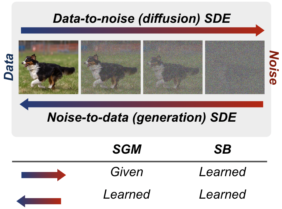
Figure 1: Both Score-based Generative Model (SGM) and Schrödinger Bridge (SB) transform between two distributions. While SGM requires pre-specifying the data-to-noise diffusion, SB instead learns the process.

Score-based Generative Model (SGM; Song et al. (2020)) is an emerging generative model class that has achieved remarkable results in synthesizing high-fidelity data (Song & Ermon, 2020; Kong et al., 2020a; b). Like many deep generative models, SGM seeks to find nonlinear functions that transform simple distributions (typically Gaussian) into complex, often intractable, data distributions. In SGM, this is done by first diffusing data to noise through a stochastic differential equation (SDE); then learning to reverse this diffusion process by regressing a network to the score function (i.e. the gradient of the log probability density) at each time step (Hyvärinen & Dayan, 2005). This reversed process thereby defines the generation (see Fig. 1).

Despite its empirical successes, SGM admits few limitations. First, the diffusion process has to obey a simple form (e.g.  linear or degenerate drift) in order to compute the analytic score function for the regression purpose. Secondly, the diffusion process needs to run to sufficiently large time steps so that the end distribution is approximate Gaussian (Kong & Ping, 2021). For these reasons, SGM often takes a notoriously long time in generating data (Jolicoeur-Martineau et al., 2021), thereby limiting their practical usages compared to e.g. GANs or flow-based models (Ping et al., 2020; Karras et al., 2020b).

In the attempt to lift these restrictions, a line of recent works inspired by Schrödinger Bridge (SB; Schrödinger (1932)) has been proposed (De Bortoli et al., 2021; Wang et al., 2021; Vargas et al., 2021). SB – as an entropy-regularized optimal transport problem – seeks two optimal policies that transform back-and-forth between two arbitrary distributions in a finite horizon. The similarity between the two problems (i.e. both involve transforming distributions) is evident, and the additional flexibility from SB is also attractive. To enable SB-inspired generative training, however, previous works require either ad-hoc multi-stage optimization or retreat to traditional SB algorithms, e.g. Iterative Proportional Fitting (IPF; Kullback (1968)). The underlying relation between the optimization principle of SB and modern generative training, in particular SGM, remains relatively unexplored, despite their intimately related problem formulations. More importantly, with the recent connection between SGM and log-likelihood computation (Song et al., 2021), it is crucial to explore whether there exists an alternative way of training SB that better respects, or perhaps generalizes, modern training of SGM, so as to solidify the suitability of SB as a principled generative model.

In this work, we present a fundamental connection between solving SB and training SGM. The difficulty arises immediately as one notices that the optimality condition of SB and the likelihood objective of SGM are represented by merely two distinct mathematical objects. While the former is characterized by two coupled partial differential equations (PDEs) (Léonard, 2013), the latter integrates over a notably complex SDE that resembles neither its diffusion nor reversed process (Song et al., 2021). Nevertheless, inspired by the recent advance on understanding deep learning through the optimal control perspective (Li & Hao, 2018; Liu et al., 2021a; b), we show that Forward-Backward SDEs – a mathematical methodology appearing in stochastic optimal control for solving nonlinear PDEs (Han et al., 2018) – paves an elegant way to connect the two objectives. The implication of our findings is nontrivial: It yields an exact log-likelihood expression of SB that precisely generalizes the one of SGM (Song et al., 2021) to fully nonlinear diffusion, thereby providing novel theoretical connections between the two model classes. Algorithmically, our framework suggests rich training procedures that resemble the joint optimization for diffusion flow-based models (Zhang & Chen, 2021) or more traditional IPF approaches (Kullback, 1968; De Bortoli et al., 2021). This allows one to marry the best of both worlds by improving the SB training with e.g. a SGM-inspired Langevin corrector (Song & Ermon, 2019). The resulting method, SB-FBSDE, generates encouraging images on MNIST, CelebA, and CIFAR10 and outperforms prior optimal transport models by a large margin.

Our method differs from the concurrent SB methods (De Bortoli et al., 2021; Vargas et al., 2021) in various aspects. First, while both prior methods rely on solving SB with mean-matching regression, our SB-FBSDE instead utilizes a divergence-based objectives (see §§\S3.2). Secondly, neither of the prior methods focuses on log-likelihood training, which is the key finding in SB-FBSDE to bridge connections to SGM and adopt modern training improvements. Indeed, due to the difference in the underlying SDE classes,111 We adopt the recent advance in SB theory (Caluya & Halder, 2021) that extends classical SB models (used in prior works) to the exact SDE class appearing in SGM. See Appendices A and C for more details. their connections to SGM can only be made after time discretization by carefully choosing each step size (De Bortoli et al., 2021). In contrast, our theoretical connection is derived readily in continuous-time; hence unaffected by the choice of numerical discretization.

In summary, we present the following contributions.

  • We present a novel computational framework, grounded on Forward-Backward SDEs theory, for computing the log-likelihood objectives of Schrödinger Bridge (SB) and solidifying their theoretical connections to Score-based Generative Model (SGM).

  • Our framework suggests a new training principle that retains the mathematical flexibility from SB while enjoying advanced techniques from the modern generative training of SGM.

  • We show that the resulting method – named SB-FBSDE – outperforms previous optimal transport-inspired baselines on synthesizing high-fidelity images and is comparable to other existing models.

Notation.

We denote ptSDE(𝐗t)superscriptsubscript𝑝𝑡SDEsubscript𝐗𝑡p_{t}^{\mathrm{SDE}}({\mathbf{X}}_{t}) as the marginal density driven by some SDESDE\mathrm{SDE} process 𝐗(t)𝐗t𝐗𝑡subscript𝐗𝑡{\mathbf{X}}(t)\equiv{\mathbf{X}}_{t} until the time step t[0,T]𝑡0𝑇t\in[0,T]. The time direction is aligned throughout this article such that p0subscript𝑝0p_{0} and pTsubscript𝑝𝑇p_{T} respectively correspond to the data and prior distributions. The gradient, divergence, and Hessian of a function f(𝒙)𝑓𝒙f({\bm{x}}), where 𝒙n𝒙superscript𝑛{\bm{x}}\in\mathbb{R}^{n}, will be denoted as 𝒙fnsubscript𝒙𝑓superscript𝑛\nabla_{\bm{x}}f\in\mathbb{R}^{n}, 𝒙fsubscript𝒙𝑓\nabla_{\bm{x}}\cdot f\in\mathbb{R}, and 𝒙2fn×nsubscriptsuperscript2𝒙𝑓superscript𝑛𝑛\nabla^{2}_{{\bm{x}}}f\in\mathbb{R}^{n\times n}.

2 Preliminaries

2.1 Score-based Generative Model (SGM)

Given a data point 𝐗0nsubscript𝐗0superscript𝑛{\mathbf{X}}_{0}\in\mathbb{R}^{n} sampled from an unknown data distribution pdatasubscript𝑝data{p_{\text{{data}}}}, SGM first progressively diffuses the data towards random noise with the following forward SDE:

d𝐗t=f(t,𝐗t)dt+g(t)d𝐖t,𝐗0pdata,formulae-sequencedsubscript𝐗𝑡𝑓𝑡subscript𝐗𝑡d𝑡𝑔𝑡dsubscript𝐖𝑡similar-tosubscript𝐗0subscript𝑝data\displaystyle{\textnormal{d}}{\mathbf{X}}_{t}=f(t,{\mathbf{X}}_{t}){\mathrm{d}t}+g(t){\mathrm{d}{\mathbf{W}_{t}}},\quad{\mathbf{X}}_{0}\sim{p_{\text{{data}}}}, (1)

where f(,t):nn:𝑓𝑡superscript𝑛superscript𝑛f(\cdot,t):\mathbb{R}^{n}\rightarrow\mathbb{R}^{n}, g(t)𝑔𝑡g(t)\in\mathbb{R}, and 𝐖tnsubscript𝐖𝑡superscript𝑛{\mathbf{W}_{t}}\in\mathbb{R}^{n} are the drift, diffusion, and standard Wiener process. Typically, g()𝑔g(\cdot) is some monotonically increasing function such that for sufficiently large time steps, we have pT(1)ppriorsuperscriptsubscript𝑝𝑇(1)subscript𝑝priorp_{T}^{\text{{(\ref{eq:fsde})}}}\approx{p_{\text{{prior}}}} resemble some prior distribution (e.g. Gaussian) at the terminal horizon T𝑇T. Reversing (1) yields another SDE222 Hereafter, we will sometimes drop ff(t,𝐗t)𝑓𝑓𝑡subscript𝐗𝑡f\equiv f(t,{\mathbf{X}}_{t}) and gg(t)𝑔𝑔𝑡g\equiv g(t) for brevity. that traverses backward in time (Anderson, 1982):

d𝐗t=[fg2𝒙logpt(1)(𝐗t)]dt+gd𝐖t,𝐗TpT(1),formulae-sequencedsubscript𝐗𝑡delimited-[]𝑓superscript𝑔2subscript𝒙superscriptsubscript𝑝𝑡(1)subscript𝐗𝑡d𝑡𝑔dsubscript𝐖𝑡similar-tosubscript𝐗𝑇superscriptsubscript𝑝𝑇(1)\displaystyle{\textnormal{d}}{\mathbf{X}}_{t}=[f-g^{2}~{}\nabla_{\bm{x}}\log p_{t}^{\text{{(\ref{eq:fsde})}}}({\mathbf{X}}_{t})]{\mathrm{d}t}+g~{}{\mathrm{d}{\mathbf{W}_{t}}},\quad{\mathbf{X}}_{T}\sim p_{T}^{\text{{(\ref{eq:fsde})}}}, (2)

where pt(1)superscriptsubscript𝑝𝑡(1)p_{t}^{\text{(\ref{eq:fsde})}} corresponds to the marginal density of SDE (1) at time t𝑡t, and 𝒙logpt(1)subscript𝒙superscriptsubscript𝑝𝑡(1)\nabla_{\bm{x}}\log p_{t}^{\text{{(\ref{eq:fsde})}}} is known as the score function. These two stochastic processes are equivalent in the sense that their marginal densities are equal to each other throughout t[0,T]𝑡0𝑇t\in[0,T]; in other words, pt(1)pt(2)superscriptsubscript𝑝𝑡(1)superscriptsubscript𝑝𝑡(2)p_{t}^{\text{{(\ref{eq:fsde})}}}\equiv p_{t}^{\text{{(\ref{eq:rsde})}}}.

When the drift f𝑓f is of simple structure, for instance linear (Ho et al., 2020) or simply degenerate (Song & Ermon, 2019), the conditional score function 𝒙logpt(1)(𝐗t|𝐗0=𝒙0)𝒙logpt|𝒙0subscript𝒙superscriptsubscript𝑝𝑡(1)conditionalsubscript𝐗𝑡subscript𝐗0subscript𝒙0subscript𝒙subscript𝑝conditional𝑡subscript𝒙0\nabla_{\bm{x}}\log p_{t}^{\text{(\ref{eq:fsde})}}({\mathbf{X}}_{t}|{\mathbf{X}}_{0}={\bm{x}}_{0})\equiv\nabla_{\bm{x}}\log p_{t|{\bm{x}}_{0}} admits an analytic solution at any time t𝑡t. Hence, SGM proposes to train a parameterized score network 𝐬(t,𝒙;θ)𝐬𝑡𝒙𝜃{\mathbf{s}}(t,{\bm{x}};\theta) by regressing its outputs to the ground-truth values, i.e. 𝔼[λ(t)𝐬(t,𝐗t;θ)𝒙logpt|𝒙02]𝔼delimited-[]𝜆𝑡superscriptdelimited-∥∥𝐬𝑡subscript𝐗𝑡𝜃subscript𝒙subscript𝑝conditional𝑡subscript𝒙02\mathbb{E}[\lambda(t)\lVert{\mathbf{s}}(t,{\mathbf{X}}_{t};\theta)-{\nabla_{\bm{x}}\log p_{t|{\bm{x}}_{0}}}\rVert^{2}], where the expectation is taken over the SDE (1). In practice, λ(t)𝜆𝑡\lambda(t) is some hand-designed weighting function that largely affects the performance. Recent works (Song et al., 2021; Huang et al., 2021) have shown that the log-likelihood of SGM, despite being complex, can be lower-bounded as follows:

logp0SGM(𝒙0)SGM(𝒙0;θ)=𝔼[logpT(𝐗T)]0T𝔼[12g2𝐬t2+𝒙(g2𝐬tf)]dt,superscriptsubscript𝑝0SGMsubscript𝒙0subscriptsuperscriptSGMsubscript𝒙0𝜃𝔼delimited-[]subscript𝑝𝑇subscript𝐗𝑇superscriptsubscript0𝑇𝔼delimited-[]12superscript𝑔2superscriptdelimited-∥∥subscript𝐬𝑡2subscript𝒙superscript𝑔2subscript𝐬𝑡𝑓differential-d𝑡\displaystyle{\log p_{0}^{\text{{SGM}}}({\bm{x}}_{0})\geq}{\cal L}^{\text{}}_{\text{SGM}}({\bm{x}}_{0};\theta)=\mathbb{E}\left[\log p_{T}({\mathbf{X}}_{T})\right]-\int_{0}^{T}\mathbb{E}\left[\frac{1}{2}g^{2}\lVert{\mathbf{s}}_{t}\rVert^{2}+\nabla_{\bm{x}}\cdot\left(g^{2}{\mathbf{s}}_{t}-f\right)\right]{\mathrm{d}t}, (3)
=𝔼[logpT(𝐗T)]0T𝔼[12g2𝐬t𝒙logpt|𝒙0212g𝒙logpt|𝒙02𝒙f]dt,absent𝔼delimited-[]subscript𝑝𝑇subscript𝐗𝑇superscriptsubscript0𝑇𝔼delimited-[]12superscript𝑔2superscriptdelimited-∥∥subscript𝐬𝑡subscript𝒙subscript𝑝conditional𝑡subscript𝒙0212superscriptdelimited-∥∥𝑔subscript𝒙subscript𝑝conditional𝑡subscript𝒙02subscript𝒙𝑓differential-d𝑡\displaystyle\qquad=\mathbb{E}\left[\log p_{T}({\mathbf{X}}_{T})\right]-\int_{0}^{T}\mathbb{E}\left[\frac{1}{2}g^{2}\lVert{\mathbf{s}}_{t}-{\nabla_{\bm{x}}\log p_{t|{\bm{x}}_{0}}}\rVert^{2}-\frac{1}{2}\lVert g{\nabla_{\bm{x}}\log p_{t|{\bm{x}}_{0}}}\rVert^{2}-\nabla_{\bm{x}}\cdot f\right]{\mathrm{d}t},

where 𝐬t𝐬(t,𝒙;θ)subscript𝐬𝑡𝐬𝑡𝒙𝜃{\mathbf{s}}_{t}\equiv{\mathbf{s}}(t,{\bm{x}};\theta) and the expectation is taken over the SDE (1) given a data point 𝐗0=𝒙0subscript𝐗0subscript𝒙0{\mathbf{X}}_{0}={\bm{x}}_{0}. This objective (3) suggests a principled choice of λ(t):=g(t)2assign𝜆𝑡𝑔superscript𝑡2\lambda(t):=g(t)^{2}. After training, SGM simply substitutes the score function with the learned score network 𝐬(t,𝒙;θ)𝐬𝑡𝒙𝜃{\mathbf{s}}(t,{\bm{x}};\theta) to generate data from ppriorsubscript𝑝prior{p_{\text{{prior}}}},

d𝐗t=[fg2𝐬(t,𝐗t;θ)]dt+gd𝐖t,𝐗Tpprior.formulae-sequencedsubscript𝐗𝑡delimited-[]𝑓superscript𝑔2𝐬𝑡subscript𝐗𝑡𝜃d𝑡𝑔dsubscript𝐖𝑡similar-tosubscript𝐗𝑇subscript𝑝prior\displaystyle{\textnormal{d}}{\mathbf{X}}_{t}=[f-g^{2}~{}{\mathbf{s}}(t,{\mathbf{X}}_{t};\theta)]{\mathrm{d}t}+g~{}{\mathrm{d}{\mathbf{W}_{t}}},\quad{\mathbf{X}}_{T}\sim{p_{\text{{prior}}}}. (4)

It is important to notice that ppriorsubscript𝑝prior{p_{\text{{prior}}}} needs not equal pT(1)superscriptsubscript𝑝𝑇(1)p_{T}^{\text{{(\ref{eq:fsde})}}} in practice, and the approximation is close only through a careful design of (1). Notably, designing the diffusion g(t)𝑔𝑡g(t) can be particularly problematic as it affects both the approximation pT(1)ppriorsuperscriptsubscript𝑝𝑇(1)subscript𝑝priorp_{T}^{\text{{(\ref{eq:fsde})}}}\approx{p_{\text{{prior}}}} and the training via the weighting λ(t)𝜆𝑡\lambda(t); hence can lead to unstable training (Nichol & Dhariwal, 2021). In contrast, Schrödinger Bridge considers a more flexible framework for designing the forward diffusion that requires minimal manipulation.

2.2 Schrödinger Bridge (SB)

Following the dynamic expression of SB (Pavon & Wakolbinger, 1991; Dai Pra, 1991), consider

min𝒫(pdata,pprior)DKL(||),\displaystyle\min_{{\mathbb{Q}}\in{\cal P}({p_{\text{{data}}}},{p_{\text{{prior}}}})}D_{\mathrm{KL}}({\mathbb{Q}}~{}||~{}{\mathbb{P}}), (5)

where 𝒫(pdata,pprior)𝒫subscript𝑝datasubscript𝑝prior{\mathbb{Q}}\in{\cal P}({p_{\text{{data}}}},{p_{\text{{prior}}}}) belongs to a set of path measure with pdatasubscript𝑝data{p_{\text{{data}}}} and ppriorsubscript𝑝prior{p_{\text{{prior}}}} as its marginal densities at t=0𝑡0t=0 and T𝑇T. On the other hand, {\mathbb{P}} denotes a reference measure, which we will set to the path measure of (1) for later convenience. The optimality condition to (5) is characterized by two PDEs that are coupled through their boundary conditions. We summarize the related result below.

Theorem 1 (SB optimality; Chen et al. (2021); Pavon & Wakolbinger (1991); Caluya & Halder (2021)).

Let Ψ(t,𝐱)Ψ𝑡𝐱\Psi(t,{\bm{x}}) and Ψ^(t,𝐱)^Ψ𝑡𝐱\widehat{\Psi}(t,{\bm{x}}) be the solutions to the following PDEs:

{Ψt=𝒙Ψ𝖳f12Tr(g2𝒙2Ψ)Ψ^t=𝒙(Ψ^f)+12Tr(g2𝒙2Ψ^)s.t. Ψ(0,)Ψ^(0,)=pdata,Ψ(T,)Ψ^(T,)=ppriorformulae-sequencecasesΨ𝑡subscript𝒙superscriptΨ𝖳𝑓12Trsuperscript𝑔2subscriptsuperscript2𝒙Ψotherwise^Ψ𝑡subscript𝒙^Ψ𝑓12Trsuperscript𝑔2subscriptsuperscript2𝒙^Ψotherwises.t. Ψ0^Ψ0subscript𝑝dataΨ𝑇^Ψ𝑇subscript𝑝prior\displaystyle\begin{cases}\frac{\partial\Psi}{\partial t}=-\nabla_{\bm{x}}\Psi^{\mathsf{T}}f{-}\frac{1}{2}\operatorname{Tr}(g^{2}\nabla^{2}_{{\bm{x}}}\Psi)\\[3.0pt] \frac{\partial\widehat{\Psi}}{\partial t}=-\nabla_{\bm{x}}\cdot(\widehat{\Psi}f){+}\frac{1}{2}\operatorname{Tr}(g^{2}\nabla^{2}_{{\bm{x}}}\widehat{\Psi})\end{cases}\text{s.t. }\Psi(0,\cdot)\widehat{\Psi}(0,\cdot)={p_{\text{{data}}}},~{}\Psi(T,\cdot)\widehat{\Psi}(T,\cdot)={p_{\text{{prior}}}} (6)

Then, the solution to the optimization (5) can be expressed by the path measure of the following forward (7a), or equivalently backward (7b), SDE:

d𝐗tdsubscript𝐗𝑡\displaystyle{\textnormal{d}}{\mathbf{X}}_{t} =[f+g2𝒙logΨ(t,𝐗t)]dt+gd𝐖t,𝐗0pdata,formulae-sequenceabsentdelimited-[]𝑓superscript𝑔2subscript𝒙Ψ𝑡subscript𝐗𝑡d𝑡𝑔dsubscript𝐖𝑡similar-tosubscript𝐗0subscript𝑝data\displaystyle=[f+g^{2}~{}\nabla_{\bm{x}}\log{\Psi}(t,{\mathbf{X}}_{t})]{\mathrm{d}t}+g~{}{\mathrm{d}{\mathbf{W}_{t}}},\quad{\mathbf{X}}_{0}\sim{p_{\text{{data}}}}, (7a)
d𝐗tdsubscript𝐗𝑡\displaystyle{\textnormal{d}}{\mathbf{X}}_{t} =[fg2𝒙logΨ^(t,𝐗t)]dt+gd𝐖t,𝐗Tpprior,formulae-sequenceabsentdelimited-[]𝑓superscript𝑔2subscript𝒙^Ψ𝑡subscript𝐗𝑡d𝑡𝑔dsubscript𝐖𝑡similar-tosubscript𝐗𝑇subscript𝑝prior\displaystyle=[f-g^{2}~{}\nabla_{\bm{x}}\log\widehat{\Psi}(t,{\mathbf{X}}_{t})]{\mathrm{d}t}+g~{}{\mathrm{d}{\mathbf{W}_{t}}},\quad{\mathbf{X}}_{T}\sim{p_{\text{{prior}}}}, (7b)

where 𝐱logΨ(t,𝐗t)subscript𝐱Ψ𝑡subscript𝐗𝑡\nabla_{\bm{x}}\log{\Psi}(t,{\mathbf{X}}_{t}) and 𝐱logΨ^(t,𝐗t)subscript𝐱^Ψ𝑡subscript𝐗𝑡\nabla_{\bm{x}}\log\widehat{\Psi}(t,{\mathbf{X}}_{t}) are the optimal forward and backward drifts for SB.

Similar to the forward/backward processes in SGM, the stochastic processes of SB in (7a) and (7b) are also equivalent in the sense that t[0,T],pt(7a)pt(7b)ptSBformulae-sequencefor-all𝑡0𝑇superscriptsubscript𝑝𝑡(7a)superscriptsubscript𝑝𝑡(7b)superscriptsubscript𝑝𝑡SB\forall t\in[0,T],~{}p_{t}^{\text{{(\ref{eq:fsb})}}}\equiv p_{t}^{\text{{(\ref{eq:bsb})}}}\equiv p_{t}^{\text{{SB}}}. In fact, its marginal density obeys a factorization principle: ptSB(𝐗t)=Ψ(t,𝐗t)Ψ^(t,𝐗t)superscriptsubscript𝑝𝑡SBsubscript𝐗𝑡Ψ𝑡subscript𝐗𝑡^Ψ𝑡subscript𝐗𝑡p_{t}^{\text{{SB}}}({\mathbf{X}}_{t})={\Psi}(t,{\mathbf{X}}_{t})\widehat{\Psi}(t,{\mathbf{X}}_{t}).

To construct the generative pipeline from (7b), one requires solving the PDEs in (6) to obtain Ψ^^Ψ\widehat{\Psi}. Unfortunately, these PDEs are hard to solve even for low-dimensional systems (Renardy & Rogers, 2006); let alone for generative applications. Indeed, previous works either have to replace the original Schrödinger Bridge (pdatappriorsubscript𝑝datasubscript𝑝prior{p_{\text{{data}}}}\leftrightarrows{p_{\text{{prior}}}}) with multiple stages, pdatapmiddleppriorsubscript𝑝datasuperscriptsubscript𝑝middlesubscript𝑝prior{p_{\text{{data}}}}\leftrightarrows p_{\text{middle}}^{\text{{}}}\leftrightarrows{p_{\text{{prior}}}}, so that each segment admits an analytic solution (Wang et al., 2021), or consider the following half-bridge (pdatappriorsubscript𝑝datasubscript𝑝prior{p_{\text{{data}}}}\leftarrow{p_{\text{{prior}}}} vs. pdatappriorsubscript𝑝datasubscript𝑝prior{p_{\text{{data}}}}\rightarrow{p_{\text{{prior}}}}) optimization (De Bortoli et al., 2021; Vargas et al., 2021),

(1):=argmin𝒫(,pprior)DKL(||(0)),(0):=argmin𝒫(pdata,)DKL(||(1))\displaystyle{\mathbb{Q}}^{(1)}:=\operatorname*{arg\,min}_{{\mathbb{Q}}\in{\cal P}(\cdot,{p_{\text{{prior}}}})}D_{\mathrm{KL}}({\mathbb{Q}}~{}||~{}{\mathbb{Q}}^{(0)}),\quad{\mathbb{Q}}^{(0)}:=\operatorname*{arg\,min}_{{\mathbb{Q}}\in{\cal P}({p_{\text{{data}}}},\cdot)}D_{\mathrm{KL}}({\mathbb{Q}}~{}||~{}{\mathbb{Q}}^{(1)})

which can be solved with IPF algorithm (Kullback, 1968) starting from (0):=assignsuperscript0{\mathbb{Q}}^{(0)}:={\mathbb{P}}. In the following section, we will present a scalable computational framework for solving the optimality PDEs in (6) and show that it paves an elegant way connecting the optimality principle of SB (6) to the parameterized log-likelihood of SGM (3).

3 Approach

Refer to caption
Figure 2: Schematic diagram of the our stochastic optimal control interpretation, and how it connects the objective of SGM (3) and optimality of SB (6) through Forward-Backward SDEs theory.

We motivate our approach starting from some control-theoretic observation (see Fig. 2). Notice that both SGM and SB consist of forward and backward SDEs with similar structures. From the stochastic control perspective, these SDEs belong to the class of control-affine SDEs with additive noise:

d𝐗t=𝑨(t,𝐗t)dt+𝑩(t,𝐗t)𝐮(t,𝐗t)dt+𝑪(t)d𝐖t.dsubscript𝐗𝑡𝑨𝑡subscript𝐗𝑡d𝑡𝑩𝑡subscript𝐗𝑡𝐮𝑡subscript𝐗𝑡d𝑡𝑪𝑡dsubscript𝐖𝑡\displaystyle{\textnormal{d}}{\mathbf{X}}_{t}={\bm{A}}(t,{\mathbf{X}}_{t}){\mathrm{d}t}+{\bm{B}}(t,{\mathbf{X}}_{t}){\mathbf{u}}(t,{\mathbf{X}}_{t}){\mathrm{d}t}+{\bm{C}}(t)~{}{\mathrm{d}{\mathbf{W}_{t}}}. (8)

It is clear that the control-affine SDE (8) includes all SDEs (1,2,4,7) appearing in §§\S2 by considering (𝑨,𝑩,𝑪):=(f,𝑰,g)assign𝑨𝑩𝑪𝑓𝑰𝑔({\bm{A}},{\bm{B}},{\bm{C}}):=(f,{\bm{I}},g) and different interpretations of the control variables 𝐮(t,𝐗t)𝐮𝑡subscript𝐗𝑡{\mathbf{u}}(t,{\mathbf{X}}_{t}). This implies that the optimization processes of both SGM and SB can be aligned through the lens of stochastic optimal control (SOC). Indeed, both problems can be interpreted as seeking some time-varying control policy, either the score function 𝒙logpt|𝒙0subscript𝒙subscript𝑝conditional𝑡subscript𝒙0{\nabla_{\bm{x}}\log p_{t|{\bm{x}}_{0}}} in SGM or 𝒙logΨ^subscript𝒙^Ψ{\nabla_{\bm{x}}\log\widehat{\Psi}} in SB, that minimizes some objectives, (3) vs. (5), while subjected to some control-affine SDEs, (1,2) vs. (7). In what follows, we will show that a specific mathematical methodology in nonlinear SOC literature – called Forward-Backward SDEs theory (FBSDEs; see Ma et al. (1999)) – links the optimality condition of SB (6) to the log-likelihood objectives of SGM (3). All proofs are left to Appendix B.

3.1 Forward-Backward SDEs (FBSDEs) Representation for SB

The theory of FBSDEs establishes an innate connection between different classes of PDEs and forward-backward SDEs. Below we introduce the following connection related to our problem.

Lemma 2 (Nonlinear Feynman-Kac;333 Lemma 2 can be viewed as the nonlinear extension of the celebrated Feynman-Kac formula (Karatzas & Shreve, 2012), which characterizes the connection between linear PDEs and forward SDEs. Exarchos & Theodorou (2018)).

Consider the coupled SDEs

d𝐗tdsubscript𝐗𝑡\displaystyle{\textnormal{d}}{\mathbf{X}}_{t} =f(t,𝐗t)dt+G(t,𝐗t)d𝐖t,  𝐗0=𝒙0formulae-sequenceabsent𝑓𝑡subscript𝐗𝑡d𝑡𝐺𝑡subscript𝐗𝑡dsubscript𝐖𝑡  subscript𝐗0subscript𝒙0\displaystyle=f(t,{\mathbf{X}}_{t}){\mathrm{d}t}+G(t,{\mathbf{X}}_{t}){\mathrm{d}{\mathbf{W}_{t}}},\qquad\qquad\quad\text{ }\text{ }{\mathbf{X}}_{0}={\bm{x}}_{0} (9a)
d𝐘tdsubscript𝐘𝑡\displaystyle{\textnormal{d}}{\mathbf{Y}}_{t} =h(t,𝐗t,𝐘t,𝐙t)dt+𝐙(t,𝐗t)𝖳d𝐖t,𝐘T=φ(𝐗T)formulae-sequenceabsent𝑡subscript𝐗𝑡subscript𝐘𝑡subscript𝐙𝑡d𝑡𝐙superscript𝑡subscript𝐗𝑡𝖳dsubscript𝐖𝑡subscript𝐘𝑇𝜑subscript𝐗𝑇\displaystyle=-h(t,{\mathbf{X}}_{t},{\mathbf{Y}}_{t},{\mathbf{Z}}_{t}){\mathrm{d}t}+{\mathbf{Z}}(t,{\mathbf{X}}_{t})^{\mathsf{T}}{\mathrm{d}{\mathbf{W}_{t}}},\quad{\mathbf{Y}}_{T}=\varphi({\mathbf{X}}_{T}) (9b)

where the functions f𝑓f, G𝐺G, hh, and φ𝜑{\varphi} satisfy proper regularity conditions444 Yong & Zhou (1999); Kobylanski (2000) require f𝑓f, G𝐺G, hh, and φ𝜑{\varphi} to be continuous, f𝑓f and G𝐺G to be uniformly Lipschitz in 𝐱𝐱{\bm{x}}, and hh to satisfy quadratic growth condition in 𝐳𝐳{\bm{z}}. so that there exists a pair of unique strong solutions satisfying (9). Now, consider the following second-order parabolic PDE and suppose v(t,𝐱)v𝑣𝑡𝐱𝑣v(t,{\bm{x}})\equiv v is once continuously differentiable in t𝑡t and twice in 𝐱𝐱{\bm{x}}, i.e. vC1,2𝑣superscript𝐶12v\in C^{1,2},

vt+12Tr(𝒙2vGG𝖳)+𝒙v𝖳f+h(t,𝒙,v,G𝖳𝒙v)=0,v(T,𝒙)=φ(𝒙),formulae-sequence𝑣𝑡12Trsubscriptsuperscript2𝒙𝑣𝐺superscript𝐺𝖳subscript𝒙superscript𝑣𝖳𝑓𝑡𝒙𝑣superscript𝐺𝖳subscript𝒙𝑣0𝑣𝑇𝒙𝜑𝒙\displaystyle\frac{\partial v}{\partial t}+\frac{1}{2}\operatorname{Tr}(\nabla^{2}_{{\bm{x}}}v~{}GG^{\mathsf{T}})+\nabla_{\bm{x}}v^{\mathsf{T}}f+h(t,{\bm{x}},v,G^{\mathsf{T}}\nabla_{\bm{x}}v)=0,\quad v(T,{\bm{x}})=\varphi({\bm{x}}), (10)

then the solution to (9) coincides with the solution to (10) along paths generated by the forward SDE (9a) almost surely, i.e., the following stochastic representation (known as the nonlinear Feynman-Kac relation) is valid:

v(t,𝐗t)=𝐘tandG(t,𝐗t)𝖳𝒙v(t,𝐗t)=𝐙t.formulae-sequence𝑣𝑡subscript𝐗𝑡subscript𝐘𝑡and𝐺superscript𝑡subscript𝐗𝑡𝖳subscript𝒙𝑣𝑡subscript𝐗𝑡subscript𝐙𝑡\displaystyle v(t,{\mathbf{X}}_{t})={\mathbf{Y}}_{t}\qquad\text{and}\qquad G(t,{\mathbf{X}}_{t})^{\mathsf{T}}\nabla_{\bm{x}}v(t,{\mathbf{X}}_{t})={\mathbf{Z}}_{t}. (11)

Lemma 2 states that solutions to a certain class of nonlinear (via the function hh in (10)) PDEs can be represented by solutions to a set of forward-backward SDEs (9) through the transformation (11), and this relation can be extended to the viscosity case (Pardoux & Peng (1992); see also Appendix B). Note that 𝐘tsubscript𝐘𝑡{\mathbf{Y}}_{t} is the solution to the backward SDE (9b) whose randomness is driven by the forward SDE (9a). Indeed, it is clear from (11) that 𝐘tsubscript𝐘𝑡{\mathbf{Y}}_{t} (hence also 𝐙tsubscript𝐙𝑡{\mathbf{Z}}_{t}) is a time-varying function of 𝐗tsubscript𝐗𝑡{\mathbf{X}}_{t}. Since the v𝑣v appearing in the nonlinear Feynman-Kac relation (11) takes the random vector 𝐗tsubscript𝐗𝑡{\mathbf{X}}_{t} as its argument, v(t,𝐗t)𝑣𝑡subscript𝐗𝑡v(t,{\mathbf{X}}_{t}) shall also be understood as a random variable. Finally, it is known that the original (deterministic) PDE solution v(t,𝒙)𝑣𝑡𝒙v(t,{\bm{x}}) can be recovered by taking conditional expectation, i.e.

v(t,𝒙)=𝔼𝐗t(9a)[𝐘t|𝐗t=𝒙]andG(t,𝒙)𝖳𝒙v(t,𝒙)=𝔼𝐗t(9a)[𝐙t|𝐗t=𝒙].formulae-sequence𝑣𝑡𝒙subscript𝔼similar-tosubscript𝐗𝑡(9a)delimited-[]conditionalsubscript𝐘𝑡subscript𝐗𝑡𝒙and𝐺superscript𝑡𝒙𝖳subscript𝒙𝑣𝑡𝒙subscript𝔼similar-tosubscript𝐗𝑡(9a)delimited-[]conditionalsubscript𝐙𝑡subscript𝐗𝑡𝒙\displaystyle v(t,{\bm{x}})=\mathbb{E}_{{\mathbf{X}}_{t}\sim\text{(\ref{eq:fbsde-f})}}[{\mathbf{Y}}_{t}|{\mathbf{X}}_{t}={\bm{x}}]\quad\text{and}\quad G(t,{\bm{x}})^{\mathsf{T}}\nabla_{\bm{x}}v(t,{\bm{x}})=\mathbb{E}_{{\mathbf{X}}_{t}\sim\text{(\ref{eq:fbsde-f})}}[{\mathbf{Z}}_{t}|{\mathbf{X}}_{t}={\bm{x}}]. (12)

Since it is often computationally favorable to solve SDEs rather than PDEs, Lemma 2 has been widely used as a scalable method for solving high-dimensional PDEs (Han et al., 2018; Pereira et al., 2019). Take SOC applications for instance, their PDE optimality condition can be characterized by (11) under proper conditions, with the optimal control given in the form of 𝐙tsubscript𝐙𝑡{\mathbf{Z}}_{t}. Hence, one can adopt Lemma 2 to solve the underlying FBSDEs, rather than the original PDE optimality, for the optimal control. Despite seemingly attractive, whether these principles can be extended to SB, whose optimality conditions are given by two coupled PDEs in (6), remains unclear. Below we derive a similar FBSDEs representation for SB.

Theorem 3 (FBSDEs to SB optimality (6)).

Consider the following set of coupled SDEs,

d𝐗tdsubscript𝐗𝑡\displaystyle{\textnormal{d}}{\mathbf{X}}_{t} =(f+g𝐙t)dt+gd𝐖tabsent𝑓𝑔subscript𝐙𝑡d𝑡𝑔dsubscript𝐖𝑡\displaystyle=\left(f+g{\mathbf{Z}}_{t}\right){\mathrm{d}t}+g{\mathrm{d}{\mathbf{W}_{t}}} (13a)
d𝐘tdsubscript𝐘𝑡\displaystyle{\textnormal{d}}{\mathbf{Y}}_{t} =12𝐙t𝖳𝐙tdt+𝐙t𝖳d𝐖tabsent12superscriptsubscript𝐙𝑡𝖳subscript𝐙𝑡d𝑡superscriptsubscript𝐙𝑡𝖳dsubscript𝐖𝑡\displaystyle=\frac{1}{2}{\mathbf{Z}}_{t}^{\mathsf{T}}{\mathbf{Z}}_{t}{\mathrm{d}t}+{\mathbf{Z}}_{t}^{\mathsf{T}}{\mathrm{d}{\mathbf{W}_{t}}} (13b)
d𝐘^tdsubscript^𝐘𝑡\displaystyle{\textnormal{d}}\widehat{{\mathbf{Y}}}_{t} =(12𝐙^t𝖳𝐙^t+𝒙(g𝐙^tf)+𝐙^t𝖳𝐙t)dt+𝐙^t𝖳d𝐖tabsent12superscriptsubscript^𝐙𝑡𝖳subscript^𝐙𝑡subscript𝒙𝑔subscript^𝐙𝑡𝑓superscriptsubscript^𝐙𝑡𝖳subscript𝐙𝑡d𝑡superscriptsubscript^𝐙𝑡𝖳dsubscript𝐖𝑡\displaystyle=\left(\frac{1}{2}\widehat{{\mathbf{Z}}}_{t}^{\mathsf{T}}\widehat{{\mathbf{Z}}}_{t}+\nabla_{\bm{x}}\cdot(g\widehat{{\mathbf{Z}}}_{t}-f)+\widehat{{\mathbf{Z}}}_{t}^{\mathsf{T}}{\mathbf{Z}}_{t}\right){\mathrm{d}t}+\widehat{{\mathbf{Z}}}_{t}^{\mathsf{T}}{\mathrm{d}{\mathbf{W}_{t}}} (13c)

where f𝑓f and g𝑔g satisfy the same regularity conditions in Lemma 2 (see Footnote 4), and the boundary conditions are given by 𝐗(0)=𝐱0𝐗0subscript𝐱0{\mathbf{X}}(0)={\bm{x}}_{0} and 𝐘T+𝐘^T=logpprior(𝐗T)subscript𝐘𝑇subscript^𝐘𝑇subscript𝑝priorsubscript𝐗𝑇{\mathbf{Y}}_{T}+\widehat{{\mathbf{Y}}}_{T}=\log{p_{\text{{prior}}}}({\mathbf{X}}_{T}). Suppose Ψ,Ψ^C1,2Ψ^Ψsuperscript𝐶12\Psi,\widehat{\Psi}\in C^{1,2}, then the nonlinear Feynman-Kac relations between the FBSDEs (13) and PDEs (6) are given by

𝐘tsubscript𝐘𝑡\displaystyle{\mathbf{Y}}_{t} 𝐘(t,𝐗t)=logΨ(t,𝐗t),𝐙tformulae-sequenceabsent𝐘𝑡subscript𝐗𝑡Ψ𝑡subscript𝐗𝑡subscript𝐙𝑡\displaystyle\equiv{\mathbf{Y}}(t,{\mathbf{X}}_{t})=\log\Psi(t,{\mathbf{X}}_{t}),\qquad{\mathbf{Z}}_{t} 𝐙(t,𝐗t)=g𝒙logΨ(t,𝐗t),absent𝐙𝑡subscript𝐗𝑡𝑔subscript𝒙Ψ𝑡subscript𝐗𝑡\displaystyle\equiv{\mathbf{Z}}(t,{\mathbf{X}}_{t})=g\nabla_{\bm{x}}\log\Psi(t,{\mathbf{X}}_{t}), (14)
𝐘^tsubscript^𝐘𝑡\displaystyle\widehat{{\mathbf{Y}}}_{t} 𝐘^(t,𝐗t)=logΨ^(t,𝐗t),𝐙^tformulae-sequenceabsent^𝐘𝑡subscript𝐗𝑡^Ψ𝑡subscript𝐗𝑡subscript^𝐙𝑡\displaystyle\equiv\widehat{{\mathbf{Y}}}(t,{\mathbf{X}}_{t})=\log\widehat{\Psi}(t,{\mathbf{X}}_{t}),\qquad\widehat{{\mathbf{Z}}}_{t} 𝐙^(t,𝐗t)=g𝒙logΨ^(t,𝐗t).absent^𝐙𝑡subscript𝐗𝑡𝑔subscript𝒙^Ψ𝑡subscript𝐗𝑡\displaystyle\equiv\widehat{{\mathbf{Z}}}(t,{\mathbf{X}}_{t})=g\nabla_{\bm{x}}\log\widehat{\Psi}(t,{\mathbf{X}}_{t}).

Furthermore, (𝐘t,𝐘^t)subscript𝐘𝑡subscript^𝐘𝑡({\mathbf{Y}}_{t},\widehat{{\mathbf{Y}}}_{t}) obey the following relation:

𝐘t+𝐘^t=logptSB(𝐗t).subscript𝐘𝑡subscript^𝐘𝑡superscriptsubscript𝑝𝑡SBsubscript𝐗𝑡\displaystyle{{\mathbf{Y}}_{t}+\widehat{{\mathbf{Y}}}_{t}}=\log p_{t}^{\text{{SB}}}({\mathbf{X}}_{t}).

The FBSDEs for SB (13) share a similar forward-backward structure as in (9), where (13a) and (13b,13c) respectively represent the forward and backward SDEs. One can verify that the forward SDE (13a) coincides with the optimal forward SDE (7a) with the substitution 𝐙t=g𝒙logΨsubscript𝐙𝑡𝑔subscript𝒙Ψ{\mathbf{Z}}_{t}=g\nabla_{\bm{x}}\log\Psi. In other words, these FBSDEs provide a local representation of logΨΨ\log\Psi and logΨ^^Ψ\log\widehat{\Psi} evaluated on the optimal path governed by (7a). Since 𝐙tsubscript𝐙𝑡{\mathbf{Z}}_{t} and 𝐙^tsubscript^𝐙𝑡\widehat{{\mathbf{Z}}}_{t} can be understood as the forward/backward policies, in a similar spirit of policy-based methods (Pereira et al., 2020; Schulman et al., 2015), that guide the SDE processes of SB, they sufficiently characterize the SB model. Hence, our next step is to derive a proper training objective to optimize these policies.

3.2 Log-likelihood Computation of SB

Theorem 3 has an important implication: It suggests that given a path sampled from the forward SDE (13a), the solutions to the backward SDEs (13b,13c) at t=0𝑡0t=0 provide an unbiased estimation of the log-likelihood of the data point 𝒙0subscript𝒙0{\bm{x}}_{0}, i.e. 𝔼[𝐘0+𝐘^0|𝐗0=𝒙0]=logp0SB(𝒙0)=logpdata(𝒙0)𝔼delimited-[]subscript𝐘0conditionalsubscript^𝐘0subscript𝐗0subscript𝒙0superscriptsubscript𝑝0SBsubscript𝒙0subscript𝑝datasubscript𝒙0\mathbb{E}\left[{\mathbf{Y}}_{0}+\widehat{{\mathbf{Y}}}_{0}|{\mathbf{X}}_{0}={\bm{x}}_{0}\right]=\log p_{0}^{\text{{SB}}}({\bm{x}}_{0})=\log{p_{\text{{data}}}}({\bm{x}}_{0}), where 𝐗tsubscript𝐗𝑡{\mathbf{X}}_{t} is sampled from (13a). We now state our main result, which makes this observation formal:

Theorem 4 (Log-likelihood of SB model).

Given the solution satisfying the FBSDE system in (13), the log-likelihood of the SB model (𝐙t,𝐙^t)subscript𝐙𝑡subscript^𝐙𝑡({\mathbf{Z}}_{t},\widehat{{\mathbf{Z}}}_{t}), at a data point 𝐱0subscript𝐱0{\bm{x}}_{0}, can be expressed as

logp0SB(𝒙0)superscriptsubscript𝑝0SBsubscript𝒙0\displaystyle\log p_{0}^{\text{{SB}}}({\bm{x}}_{0}) =𝔼[logpT(𝐗T)]0T𝔼[12𝐙t2+12𝐙^tg𝒙logptSB+𝐙t2\displaystyle=\mathbb{E}\left[\log p_{T}({\mathbf{X}}_{T})\right]{-}\int_{0}^{T}\mathbb{E}\left[\frac{1}{2}\lVert{\mathbf{Z}}_{t}\rVert^{2}{+}\frac{1}{2}\lVert\widehat{{\mathbf{Z}}}_{t}-g\nabla_{\bm{x}}\log p_{t}^{\text{{SB}}}+{\mathbf{Z}}_{t}\rVert^{2}\right.
12g𝒙logptSB𝐙t2𝒙f]dt\displaystyle\qquad\qquad\qquad\qquad\qquad\quad\qquad\qquad\left.{-}\frac{1}{2}\lVert g\nabla_{\bm{x}}\log p_{t}^{\text{{SB}}}-{\mathbf{Z}}_{t}\rVert^{2}{-}\nabla_{\bm{x}}\cdot f\right]{\mathrm{d}t} (15)
=𝔼[logpT(𝐗T)]0T𝔼[12𝐙t2+12𝐙^t2+𝒙(g𝐙^tf)+𝐙^t𝖳𝐙t]dt,absent𝔼delimited-[]subscript𝑝𝑇subscript𝐗𝑇superscriptsubscript0𝑇𝔼delimited-[]12superscriptdelimited-∥∥subscript𝐙𝑡212superscriptdelimited-∥∥subscript^𝐙𝑡2subscript𝒙𝑔subscript^𝐙𝑡𝑓superscriptsubscript^𝐙𝑡𝖳subscript𝐙𝑡differential-d𝑡\displaystyle=\mathbb{E}\left[\log p_{T}({\mathbf{X}}_{T})\right]-\int_{0}^{T}\mathbb{E}\left[\frac{1}{2}\lVert{\mathbf{Z}}_{t}\rVert^{2}{+}\frac{1}{2}\lVert\widehat{{\mathbf{Z}}}_{t}\rVert^{2}+\nabla_{\bm{x}}\cdot(g\widehat{{\mathbf{Z}}}_{t}-f)+\widehat{{\mathbf{Z}}}_{t}^{\mathsf{T}}{{\mathbf{Z}}}_{t}\right]{\mathrm{d}t}, (16)

where the expectation is taken over the forward SDE (13a) with the initial condition 𝐗0=𝐱0subscript𝐗0subscript𝐱0{\mathbf{X}}_{0}={\bm{x}}_{0}.

Similar to (3), Theorem 4 suggests a parameterized lower bound to the log-likelihoods, i.e. logp0SB(𝒙0)SB(𝒙0;θ,ϕ)superscriptsubscript𝑝0SBsubscript𝒙0subscriptsuperscriptSBsubscript𝒙0𝜃italic-ϕ\log p_{0}^{\text{{SB}}}({\bm{x}}_{0})\geq{{\cal L}^{\text{}}_{\text{{SB}}}}({\bm{x}}_{0};\theta,\phi) where SB(𝒙0;θ,ϕ)subscriptsuperscriptSBsubscript𝒙0𝜃italic-ϕ{{\cal L}^{\text{}}_{\text{{SB}}}}({\bm{x}}_{0};\theta,\phi) shares the same expression in (16) except that 𝐙t𝐙(t,𝒙;θ)subscript𝐙𝑡𝐙𝑡𝒙𝜃{\mathbf{Z}}_{t}\approx{\mathbf{Z}}(t,{\bm{x}};\theta) and 𝐙^t𝐙^(t,𝒙;ϕ)subscript^𝐙𝑡^𝐙𝑡𝒙italic-ϕ\widehat{{\mathbf{Z}}}_{t}\approx\widehat{{\mathbf{Z}}}(t,{\bm{x}};\phi) are approximated with some parameterized models (e.g. DNNs). Note that 𝒙logptSBsubscript𝒙superscriptsubscript𝑝𝑡SB\nabla_{\bm{x}}\log p_{t}^{\text{{SB}}} is intractable in practice for any nontrivial (𝐙t,𝐙^t)subscript𝐙𝑡subscript^𝐙𝑡({\mathbf{Z}}_{t},\widehat{{\mathbf{Z}}}_{t}). Hence, we use the divergence-based objective in (16) as our training objective of both policies.

Connection to score-based models. Recall Fig. 2 and compare the parameterized log-likelihoods of SB (16) to SGM (3); one can verify that SBsubscriptsuperscriptSB{{\cal L}^{\text{}}_{\text{{SB}}}} collapses to SGMsubscriptsuperscriptSGM{{\cal L}^{\text{}}_{\text{{SGM}}}} when (𝐙t,𝐙^t):=(𝟎,g𝐬t)assignsubscript𝐙𝑡subscript^𝐙𝑡0𝑔subscript𝐬𝑡({\mathbf{Z}}_{t},\widehat{{\mathbf{Z}}}_{t}):=(\mathbf{0},g~{}{\mathbf{s}}_{t}). From the SB perspective, this occurs only when pT(1)=ppriorsuperscriptsubscript𝑝𝑇(1)subscript𝑝priorp_{T}^{\text{{(\ref{eq:fsde})}}}={p_{\text{{prior}}}}. Since no effort is required in the forward process to reach ppriorsubscript𝑝prior{p_{\text{{prior}}}}, the optimal forward control 𝐙tsubscript𝐙𝑡{\mathbf{Z}}_{t}, by definition, degenerates; thereby making the backward control 𝐙^tsubscript^𝐙𝑡\widehat{{\mathbf{Z}}}_{t} collapses to the score function. However, in any case when pT(1)ppriorsuperscriptsubscript𝑝𝑇(1)subscript𝑝priorp_{T}^{\text{{(\ref{eq:fsde})}}}\neq{p_{\text{{prior}}}}, for instance when the diffusion SDEs are improperly designed, the forward policy 𝐙tsubscript𝐙𝑡{\mathbf{Z}}_{t} steers the diffusion process back to ppriorsubscript𝑝prior{p_{\text{{prior}}}}, while its backward counterpart 𝐙^tsubscript^𝐙𝑡\widehat{{\mathbf{Z}}}_{t} compensates the reversed process accordingly. From this view, SB alleviates the problematic design in SGM by enlarging the class of diffusion processes to accept nonlinear drifts and providing an optimization principle on learning these processes. Moreover, Theorem 4 generalizes the log-likelihood training from SGM to SB.

Connection to flow-based models. Interestingly, the log-likelihood computation in Theorem 4, where we use a path {𝐗t}t[0,T]subscriptsubscript𝐗𝑡𝑡0𝑇\{{\mathbf{X}}_{t}\}_{t\in[0,T]} sampled from a data point 𝐗0subscript𝐗0{\mathbf{X}}_{0} to parameterize its log-likelihood, resembles modern training of (deterministic) flow-based models (Grathwohl et al., 2018), which have recently been shown to admit a close relation to SGM (Song et al., 2020; Gong & Li, 2021). The connection is built on the concept of probability flow – which suggests that the marginal density of an SDE can be evaluated through an ordinary differential equation (ODE). Below, we provide a similar flow representation for SB, further strengthening their connection to modern generative models.

Corollary 5 (Probability flow for SB).

The following ODE characterizes the probability flow of the optimal processes of SB (7) in the sense that t,pt(17)pt(7)ptSBfor-all𝑡superscriptsubscript𝑝𝑡(17)superscriptsubscript𝑝𝑡(7)superscriptsubscript𝑝𝑡SB\forall t,~{}p_{t}^{\text{{(\ref{eq-sb-prob})}}}\equiv p_{t}^{\text{{(\ref{eq:sb-sde})}}}\equiv p_{t}^{\text{{SB}}}.

d𝐗t=[f+g𝐙(t,𝐗t)12g(𝐙(t,𝐗t)+𝐙^(t,𝐗t))]dtdsubscript𝐗𝑡delimited-[]𝑓𝑔𝐙𝑡subscript𝐗𝑡12𝑔𝐙𝑡subscript𝐗𝑡^𝐙𝑡subscript𝐗𝑡d𝑡\displaystyle{\textnormal{d}}{\mathbf{X}}_{t}=\left[f+g{\mathbf{Z}}(t,{\mathbf{X}}_{t})-\frac{1}{2}g~{}({\mathbf{Z}}(t,{\mathbf{X}}_{t})+\widehat{{\mathbf{Z}}}(t,{\mathbf{X}}_{t}))\right]{\mathrm{d}t} (17)

One can verify (see Remark 10 in §§\SB) that computing the log-likelihood of this ODE model (17) using flow-based training techniques indeed recovers the training objective of SB derived in (16).

3.3 Practical Implementation

In this section, we detail the implementation of our FBSDE-inspired SB model, named SB-FBSDE.

Training process. We treat the log-likelihood in (16) as our training objective, where the divergence can be can be estimated efficiently following Hutchinson (1989). This immediately distinguishes SB-FBSDE from prior SB models (De Bortoli et al., 2021; Vargas et al., 2021), which instead rely on regression-based objectives.555 In fact, their regression targets may be recovered from (15) under proper transformation; see Appendix C. For low-dimensional datasets, we simply perform joint optimization, maxSB(𝒙0;θ,ϕ)subscriptsuperscriptSBsubscript𝒙0𝜃italic-ϕ\max{{\cal L}^{\text{}}_{\text{{SB}}}}({\bm{x}}_{0};\theta,\phi), to train the parameterized policies 𝐙(,;θ)𝐙𝜃{\mathbf{Z}}(\cdot,\cdot;\theta) and 𝐙^(,;ϕ)^𝐙italic-ϕ\widehat{{\mathbf{Z}}}(\cdot,\cdot;\phi). For higher-dimensional (e.g. image) datasets, however, it can be prohibitively expensive to keep the entire computational graph. In these cases, we follow De Bortoli et al. (2021) by caching the sampled trajectories in a reply buffer and refreshing them in a lower frequency basis (around 1500 iterations). Although this implies that the gradient path w.r.t. θ𝜃\theta will be discarded, we can leverage the symmetric structure of SB and re-derive the log-likelihood for the sampled noise, i.e. SB(𝒙T)subscriptsuperscriptSBsubscript𝒙𝑇{{\cal L}^{\text{}}_{\text{{SB}}}}({\bm{x}}_{T}), based on the backward trajectories sampled from (7b). We leave the derivation to Theorem 11 in §§\SB due to space constraint. This results in an alternate training between the following two objectives after dropping all unrelated terms,

~SB(𝒙0;ϕ)=0T𝔼𝐗t(7a)[12𝐙^(t,𝐗t;ϕ)2+g𝒙𝐙^(t,𝐗t;ϕ)+𝐙t𝖳𝐙^(t,𝐗t;ϕ)]dt,subscriptsuperscript~SBsubscript𝒙0italic-ϕsuperscriptsubscript0𝑇subscript𝔼similar-tosubscript𝐗𝑡(7a)delimited-[]12superscriptdelimited-∥∥^𝐙𝑡subscript𝐗𝑡italic-ϕ2𝑔subscript𝒙^𝐙𝑡subscript𝐗𝑡italic-ϕsuperscriptsubscript𝐙𝑡𝖳^𝐙𝑡subscript𝐗𝑡italic-ϕdifferential-d𝑡\displaystyle{\widetilde{{\cal L}}^{\text{}}_{\text{{SB}}}}({\bm{x}}_{0};\phi)=-\int_{0}^{T}\mathbb{E}_{{\mathbf{X}}_{t}\sim\text{(\ref{eq:fsb})}}\left[\frac{1}{2}\lVert\widehat{{\mathbf{Z}}}(t,{\mathbf{X}}_{t};\phi)\rVert^{2}+g\nabla_{\bm{x}}\cdot\widehat{{\mathbf{Z}}}(t,{\mathbf{X}}_{t};\phi)+{{\mathbf{Z}}}_{t}^{\mathsf{T}}\widehat{{\mathbf{Z}}}(t,{\mathbf{X}}_{t};\phi)\right]{\mathrm{d}t}, (18)
~SB(𝒙T;θ)=0T𝔼𝐗t(7b)[12𝐙(t,𝐗t;θ)2+g𝒙𝐙(t,𝐗t;θ)+𝐙^t𝖳𝐙(t,𝐗t;θ)]dt.subscriptsuperscript~SBsubscript𝒙𝑇𝜃superscriptsubscript0𝑇subscript𝔼similar-tosubscript𝐗𝑡(7b)delimited-[]12superscriptdelimited-∥∥𝐙𝑡subscript𝐗𝑡𝜃2𝑔subscript𝒙𝐙𝑡subscript𝐗𝑡𝜃subscriptsuperscript^𝐙𝖳𝑡𝐙𝑡subscript𝐗𝑡𝜃differential-d𝑡\displaystyle{\widetilde{{\cal L}}^{\text{}}_{\text{{SB}}}}({\bm{x}}_{T};\theta)=-\int_{0}^{T}\mathbb{E}_{{\mathbf{X}}_{t}\sim\text{(\ref{eq:bsb})}}\left[\frac{1}{2}\lVert{\mathbf{Z}}(t,{\mathbf{X}}_{t};\theta)\rVert^{2}+g\nabla_{\bm{x}}\cdot{{\mathbf{Z}}}(t,{\mathbf{X}}_{t};\theta)+\widehat{{\mathbf{Z}}}^{\mathsf{T}}_{t}{{\mathbf{Z}}}(t,{\mathbf{X}}_{t};\theta)\right]{\mathrm{d}t}. (19)

Our training process is summarized in Alg. 1. While the joint training scheme in Alg. 2 resembles recent diffusion flow-based models (Zhang & Chen, 2021), the alternate training in Alg. 3 relates to the classical IPF (De Bortoli et al., 2021), despite differing in the underlying objectives. Empirically, the joint training scheme can converge faster yet at the cost of introducing memory complexity. We highlight these flexible training procedures arising from the unified viewpoint provided in Theorem 4. Hereafter, we refer to each cycle, i.e. 2K2𝐾2K training steps, in Alg. 3 as a training stage of SB-FBSDE.

Algorithm 1 Likelihood training of SB-FBSDE
  Input: boundary distributions pdatasubscript𝑝data{p_{\text{{data}}}} and ppriorsubscript𝑝prior{p_{\text{{prior}}}},     parameterized policies 𝐙(,;θ)𝐙𝜃{\mathbf{Z}}(\cdot,\cdot;\theta) and 𝐙^(,;ϕ)^𝐙italic-ϕ\widehat{{\mathbf{Z}}}(\cdot,\cdot;\phi)
  repeat
     if  memory resource is affordable  then
        run Algorithm 2.
     else
        run Algorithm 3.
     end if
  until  converges
Algorithm 2 Joint (diffusion flow-based) training
  for k=1𝑘1k=1 to K𝐾K  do
     Sample 𝐗t[0,T]subscript𝐗𝑡0𝑇{\mathbf{X}}_{t\in[0,T]} from (13a) where 𝒙0pdatasimilar-tosubscript𝒙0subscript𝑝data{\bm{x}}_{0}\sim{p_{\text{{data}}}} (computational graph retained).
     Compute SB(𝒙0;θ,ϕ)subscriptsuperscriptSBsubscript𝒙0𝜃italic-ϕ{{\cal L}^{\text{}}_{\text{{SB}}}}({\bm{x}}_{0};\theta,\phi) with (16).
     Update (θ,ϕ)𝜃italic-ϕ(\theta,\phi) with θ,ϕSB(𝒙0;θ,ϕ)subscript𝜃italic-ϕsubscriptsuperscriptSBsubscript𝒙0𝜃italic-ϕ\nabla_{\theta,\phi}{{\cal L}^{\text{}}_{\text{{SB}}}}({\bm{x}}_{0};\theta,\phi).
  end for
Algorithm 3 Alternate (IPF-based) training
  Input: Caching frequency M𝑀M
  for k=1𝑘1k=1 to K𝐾K  do
     if  k%Mpercent𝑘𝑀k\%M == 0  then
        Sample 𝐗t[0,T]subscript𝐗𝑡0𝑇{\mathbf{X}}_{t\in[0,T]} from (13a) where 𝒙0pdatasimilar-tosubscript𝒙0subscript𝑝data{\bm{x}}_{0}\sim{p_{\text{{data}}}} (computational graph discarded).
     end if
     Compute ~SB(𝒙0;ϕ)subscriptsuperscript~SBsubscript𝒙0italic-ϕ{\widetilde{{\cal L}}^{\text{}}_{\text{{SB}}}}({\bm{x}}_{0};\phi) with (18).
     Update ϕitalic-ϕ\phi with gradient ϕ~SB(𝒙0;ϕ)subscriptitalic-ϕsubscriptsuperscript~SBsubscript𝒙0italic-ϕ\nabla_{\phi}{\widetilde{{\cal L}}^{\text{}}_{\text{{SB}}}}({\bm{x}}_{0};\phi).
  end for
  for k=1𝑘1k=1 to K𝐾K  do
     if  k%Mpercent𝑘𝑀k\%M == 0  then
        Sample 𝐗t[0,T]subscript𝐗𝑡0𝑇{\mathbf{X}}_{t\in[0,T]} from (7b) where 𝒙Tppriorsimilar-tosubscript𝒙𝑇subscript𝑝prior{\bm{x}}_{T}\sim{p_{\text{{prior}}}} (computational graph discarded).
     end if
     Compute SB(𝒙T;θ)subscriptsuperscriptSBsubscript𝒙𝑇𝜃{{\cal L}^{\text{}}_{\text{{SB}}}}({\bm{x}}_{T};\theta) with (19).
     Update θ𝜃\theta with gradient θ~SB(𝒙T;θ)subscript𝜃subscriptsuperscript~SBsubscript𝒙𝑇𝜃\nabla_{\theta}{\widetilde{{\cal L}}^{\text{}}_{\text{{SB}}}}({\bm{x}}_{T};\theta).
  end for

Generative process. While the generative processes for SB can be performed as simply as propagating (7b) given the trained policy 𝐙^(,;ϕ)^𝐙italic-ϕ\widehat{{\mathbf{Z}}}(\cdot,\cdot;\phi), it has been constantly observed that adopting Langevin sampling to the generative process greatly improves performance (Song et al., 2020). This procedure, often referred to as the Langevin corrector, requires knowing the score function 𝒙logptsubscript𝒙superscriptsubscript𝑝𝑡\nabla_{\bm{x}}\log p_{t}^{\text{{}}}. For SB, we can estimate its value by recalling (see §§\S2.2) that 𝐙t+𝐙^t=g𝒙logptSBsubscript𝐙𝑡subscript^𝐙𝑡𝑔subscript𝒙superscriptsubscript𝑝𝑡SB{\mathbf{Z}}_{t}+\widehat{{\mathbf{Z}}}_{t}=g\nabla_{\bm{x}}\log p_{t}^{\text{{SB}}}. This results in the following predictor-corrector sampling procedure (see Alg. 4 in Appendix D for more details).

Predict step:𝐗tPredict step:subscript𝐗𝑡\displaystyle\text{Predict step:}\quad{\mathbf{X}}_{t} 𝐗t+g𝐙^tΔt+gΔt ϵabsentsubscript𝐗𝑡𝑔subscript^𝐙𝑡Δ𝑡gΔt italic-ϵ\displaystyle\leftarrow{\mathbf{X}}_{t}+g~{}\widehat{{\mathbf{Z}}}_{t}\Delta t+\mathchoice{{\hbox{$\displaystyle\sqrt{g\Delta t\,}$}\lower 0.4pt\hbox{\vrule height=6.83331pt,depth=-5.46667pt}}}{{\hbox{$\textstyle\sqrt{g\Delta t\,}$}\lower 0.4pt\hbox{\vrule height=6.83331pt,depth=-5.46667pt}}}{{\hbox{$\scriptstyle\sqrt{g\Delta t\,}$}\lower 0.4pt\hbox{\vrule height=4.78333pt,depth=-3.82668pt}}}{{\hbox{$\scriptscriptstyle\sqrt{g\Delta t\,}$}\lower 0.4pt\hbox{\vrule height=3.41666pt,depth=-2.73334pt}}}{\epsilon} (20)
Correct step:𝐗tCorrect step:subscript𝐗𝑡\displaystyle\text{Correct step:}\quad{\mathbf{X}}_{t} 𝐗t+σtg(𝐙t+𝐙^t)+2σt ϵabsentsubscript𝐗𝑡subscript𝜎𝑡𝑔subscript𝐙𝑡subscript^𝐙𝑡2σt italic-ϵ\displaystyle\leftarrow{\mathbf{X}}_{t}+\textstyle\frac{\sigma_{t}}{g}({{\mathbf{Z}}}_{t}+\widehat{{\mathbf{Z}}}_{t})+\mathchoice{{\hbox{$\displaystyle\sqrt{2\sigma_{t}\,}$}\lower 0.4pt\hbox{\vrule height=6.44444pt,depth=-5.15558pt}}}{{\hbox{$\textstyle\sqrt{2\sigma_{t}\,}$}\lower 0.4pt\hbox{\vrule height=6.44444pt,depth=-5.15558pt}}}{{\hbox{$\scriptstyle\sqrt{2\sigma_{t}\,}$}\lower 0.4pt\hbox{\vrule height=4.51111pt,depth=-3.6089pt}}}{{\hbox{$\scriptscriptstyle\sqrt{2\sigma_{t}\,}$}\lower 0.4pt\hbox{\vrule height=3.22221pt,depth=-2.57779pt}}}{\epsilon} (21)

where ϵ𝒩(𝟎,𝑰)similar-toitalic-ϵ𝒩0𝑰{\epsilon}\sim{\cal N}(\mathbf{0},{\bm{I}}) and σtsubscript𝜎𝑡\sigma_{t} is the pre-specified noise scales (see (59) in Appendix D).

Limitations & efficiency. The main computational burden of our method comes from the computation of the divergence and maintaining two distinct networks. Despite it typically increases the memory by 2similar-to\sim2.5 times compared to SGM, we empirically observe that the divergence-based training converges much faster per iteration than standard regression. As a result, SB-FBSDE admits comparable training time (+6.8% in our CIFAR10 experiment) compared to SGM, yet with a substantially fewer sampling time (-80%) due to adopting nonlinear SDEs.

4 Experiments
Refer to caption
(a) GMM
Refer to caption
(b) Checkerboard
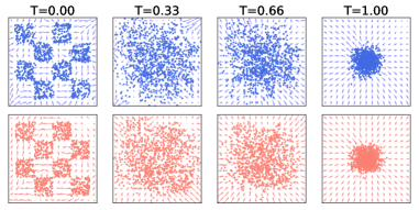
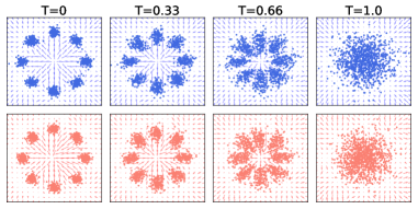
Figure 3: Validation of our SB-FBSDE model on two synthetic toy datasets that represent continuous and discontinuous distributions. Upper: Generation (pdatappriorsubscript𝑝datasubscript𝑝prior\color[rgb]{0,0.25,0.75}\definecolor[named]{pgfstrokecolor}{rgb}{0,0.25,0.75}{p_{\text{{data}}}}\leftarrow{p_{\text{{prior}}}}) process with the backward vector field 𝐙^(,;ϕ)^𝐙italic-ϕ\color[rgb]{0,0.25,0.75}\definecolor[named]{pgfstrokecolor}{rgb}{0,0.25,0.75}\widehat{{\mathbf{Z}}}(\cdot,\cdot;\phi). Bottom: Diffusion (pdatappriorsubscript𝑝datasubscript𝑝prior\color[rgb]{0.8,0,0}\definecolor[named]{pgfstrokecolor}{rgb}{0.8,0,0}{p_{\text{{data}}}}\rightarrow{p_{\text{{prior}}}}) process with the forward vector field 𝐙(,;θ)𝐙𝜃\color[rgb]{0.8,0,0}\definecolor[named]{pgfstrokecolor}{rgb}{0.8,0,0}{{\mathbf{Z}}}(\cdot,\cdot;\theta).
Refer to caption
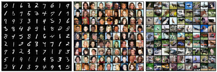
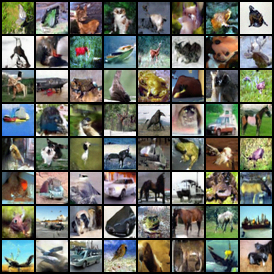
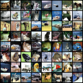
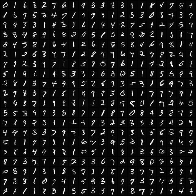
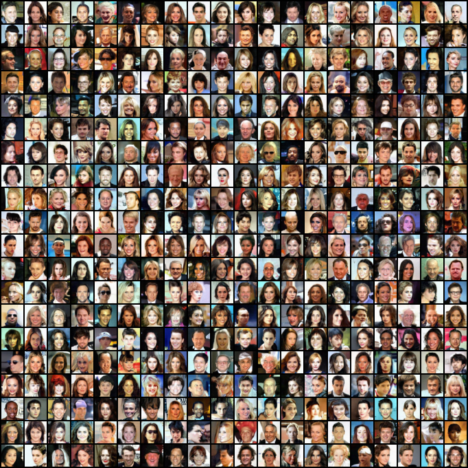
Figure 4: Uncurated samples from our SB-FBSDE models trained on MNIST (left), resized CelebA (middle) and CIFAR10 (right). More images can be found in Appendix E.

Setups. We testify SB-FBSDE on two toy datasets and three image datasets, i.e. MNIST, CelebA,666 We follow a similar setup of prior SB models (De Bortoli et al., 2021) and resize the image size to 32. and CIFAR10. ppriorsubscript𝑝prior{p_{\text{{prior}}}} is set to a zero-mean Gaussian whose variance varies for each task and can be computed according to Song & Ermon (2020). We parameterize 𝐙(,;θ)𝐙𝜃{{\mathbf{Z}}}(\cdot,\cdot;\theta) and 𝐙^(,;ϕ)^𝐙italic-ϕ\widehat{{\mathbf{Z}}}(\cdot,\cdot;\phi) with residual-based networks for toy datasets and consider Unet (Ronneberger et al., 2015) and NCSN++ (Song et al., 2020) respectively for MNIST/CelebA and CIFAR10. All networks adopt position encoding and are trained with AdamW (Loshchilov & Hutter, 2017) on a TITAN RTX. We adopt VE-SDE (i.e. f:=𝟎assign𝑓0f:=\mathbf{0}; see Song et al. (2020)) as our SDE backbone, which implies that in order to achieve reasonable performance, SB must learn a proper data-to-noise diffusion process. On all datasets, we set the horizon T=𝑇absentT=1.0 and solve the SDEs via the Euler-Maruyama method. The interval [0,T]0𝑇[0,T] is discretized into 200 steps for CIFAR10 and 100 steps for all other datasets, which are much fewer than the ones in SGM (\geq1000 steps). Other details are left in Appendix D.

Toy datasets. We first validate our joint optimization (i.e. Alg 2) on generating a mixture of Gaussian and checkerboard (adopted from Grathwohl et al. (2018)) as the representatives of continuous and discontinuous distributions. Figure 4 shows how the learned policies, i.e. 𝐙(,;θ)𝐙𝜃\color[rgb]{0.8,0,0}\definecolor[named]{pgfstrokecolor}{rgb}{0.8,0,0}{{\mathbf{Z}}}(\cdot,\cdot;\theta) and 𝐙^(,;ϕ)^𝐙italic-ϕ\color[rgb]{0,0.25,0.75}\definecolor[named]{pgfstrokecolor}{rgb}{0,0.25,0.75}\widehat{{\mathbf{Z}}}(\cdot,\cdot;\phi), construct the vector fields that progressively transport samples back-and-forth between ppriorsubscript𝑝prior{p_{\text{{prior}}}} and pdatasubscript𝑝data{p_{\text{{data}}}}. The vector fields can be highly nonlinear and dissimilar to each other. This resembles neither SGMs, whose forward vector field must obey linear structure, nor flow-based models, whose vector fields are simply with opposite directions. We highlight this as a distinct feature arising from SB models.

Image datasets. Next, we validate our alternate training (i.e. Alg 3) on high-dimensional image generation. The generated images for MNIST, CelebA, and CIFAR10 are presented in Fig. 4, which clearly suggest that our SB-FBSDE is able to synthesize high-fidelity images. More uncurated images can be founded in Appendix E. Regarding the quantitative evaluation, Table 5 summarizes the negative log-likelihood (NLL; measured in bits/dim) and the Fréchet Inception Distance score (FID; Heusel et al. (2017)) on CIFAR10. For our SB-FBSDE, we compute the NLL on the test set using Corollary 5, in a similar vein to SGMs and flow-based models, and report the FID over 50k samples w.r.t the training set. Notably, our SB-FBSDE achieves 2.98 bits/dim and 3.18 FID score on CIFAR10, which is comparable to the top existing methods from other model classes (e.g. SGMs) and outperforms prior Optimal Transport (OT) methods (Wang et al., 2021; Tanaka, 2019) by a large margin in terms of the sample quality. More importantly, it enables log-likelihood computations that are otherwise infeasible in prior OT methods. We note that the quantitative comparisons on MNIST and CelebA are omitted as the scores on these two datasets are not widely reported and different pre-processing (e.g. resizing of CelebA) can lead to values that are not directly comparable.

Figure 5: CIFAR10 evaluation using negative log-likelihood (NLL; bits/dim) on the test set and sample quality (FID score) w.r.t. the training set. Our SB-FBSDE outperforms other optimal transport baselines by a large margin and is comparable to existing generative models.
Model Class Method NLL \downarrow FID \downarrow
Optimal Transport SB-FBSDE (ours) 2.96 3.01
DOT (Tanaka, 2019) - 15.78
Multi-stage SB (Wang et al., 2021) - 12.32
DGflow (Ansari et al., 2020) - 9.63
SGMs SDE (deep, sub-VP; Song et al. (2020)) 2.99 2.92
ScoreFlow (Song et al., 2021) 2.74 5.7
VDM (Kingma et al., 2021) 2.49 4.00
LSGM(Vahdat et al., 2021) 3.43 2.10
Refer to caption
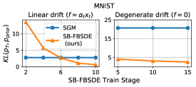
Figure 6: Validation of our SB-FBSDE on learning forward diffusions that are closer (in KL sense) to ppriorsubscript𝑝prior{p_{\text{{prior}}}} compared to SGM.
Refer to caption
Figure 7: Ablation analysis where we show that adding Langevin corrector to SB-FBSDE uniformly improves the FID scores on both CelebA and CIFAR10 training.

Validity of SB forward diffusion. Our theoretical analysis in §§\S3.2 suggests that the forward policy 𝐙(,;θ)𝐙θ𝐙𝜃subscript𝐙𝜃{{\mathbf{Z}}}(\cdot,\cdot;\theta)\equiv{\mathbf{Z}}_{\theta} plays an essential role in governing samples towards ppriorsubscript𝑝prior{p_{\text{{prior}}}}. Here, we validate this conjecture by computing the KL divergence between the terminal distribution induced by 𝐙θsubscript𝐙𝜃{\mathbf{Z}}_{\theta}, i.e. pT(13a)superscriptsubscript𝑝𝑇(13a)p_{T}^{\text{{(\ref{eq:fsde-is})}}}, and the designated prior ppriorsubscript𝑝prior{p_{\text{{prior}}}}. We refer readers to Appendix D for the actual computation. Figure 7 reports these values over MNIST training. For both degenerate (f:=𝟎assign𝑓0f:=\mathbf{0}) and linear (f:=αt𝐗tassign𝑓subscript𝛼𝑡subscript𝐗𝑡f:=\alpha_{t}{\mathbf{X}}_{t}) base drifts, our SB-FBSDE generates terminal distributions that are much closer to ppriorsubscript𝑝prior{p_{\text{{prior}}}}. Note that the values of SGM remain unchanged throughout training since SGM relies on pre-specified diffusion. This is in contrast to our SB-FBSDE whose forward policy 𝐙θsubscript𝐙𝜃{\mathbf{Z}}_{\theta} gradually shortens the KL gap to ppriorsubscript𝑝prior{p_{\text{{prior}}}}, thereby providing a better forward diffusion for training the backward policy.

Effect of Langevin corrector. In practice, we observe that the Langevin corrector greatly affects the generative performance. As shown in Fig. 7, including these corrector steps uniformly improves the sample quality (FID) on both CelebA and CIFAR10 throughout training. Since the SDEs are often solved via the Euler-Maruyama method, their propagation can be subjected to discretization errors accumulated over time. These Langevin steps thereby help re-distributing the samples at each time step t𝑡t towards the desired density ptSBsuperscriptsubscript𝑝𝑡SBp_{t}^{\text{{SB}}}. We emphasize this improvement as the benefit gained from applying modern generative training techniques based on the solid connection between SB and SGM.

5 Conclusion

In this work, we present a novel computational framework, grounded on Forward-Backward SDEs theory, for computing the log-likelihood of Schrödinger Bridge (SB) – a recently emerging model that adopts entropy-regularized optimal transport for generative modeling. Our findings provide new theoretical insights by generalizing previous theoretical results for Score-based Generative Model, and facilitate applications of modern generative training for SB. We validate our method on various image generative tasks, e.g. MNIST, CelebA, and CIFAR10, showing encouraging results in synthesizing high-fidelity samples while retaining the rigorous mathematical framework.

Acknowledgments

The authors would like to thank Ioannis Exarchos and Oswin So for their generous involvement and helpful supports during the rebuttal. The authors would also like to thank Marcus A Pereira and Ethan N Evans for their participation and kind discussion in the early stage of project exploration. This research was supported by the ARO Award # W911NF2010151.

Author Contributions

The original idea of solving the PDE optimality of SB with FBSDEs theory was initiated by Tianrong. Later, Guan derived the main theories (i.e. Theorem 3411, and Corollary 5) presented in Section 3.1, 3.2 and Appendix B with few helps from Tianrong. Tianrong designed the practical algorithms (e.g. stage-wise optimization and Langevin-corrector) in Section 3.3 and conducted most experiments with few helps from Guan. Guan wrote the main paper except for Section 4, which were written by both Tianrong and Guan. Both Guan and Tianrong contributed to code development.

Reproducibility Statement

Our training algorithms are detailed in Alg. 1, 2, and 3, with the training objectives given in the same section (see (16, 18, 19)). Other implementation details (e.g. data pre-processing) are left in Appendix D. This shall provide sufficient information for readers of interests to reproduce our results. As we strongly believe in the merit of open sourcing, we intend to release our implementation upon publication. On the theoretical side, all proofs are left to Appendix B due to space constraint. We provide the assumptions in the same section.

References

  • Anderson (1982) Brian DO Anderson. Reverse-time diffusion equation models. Stochastic Processes and their Applications, 12(3):313–326, 1982.
  • Ansari et al. (2020) Abdul Fatir Ansari, Ming Liang Ang, and Harold Soh. Refining deep generative models via discriminator gradient flow. arXiv preprint arXiv:2012.00780, 2020.
  • Caluya & Halder (2021) Kenneth Caluya and Abhishek Halder. Wasserstein proximal algorithms for the schrödinger bridge problem: Density control with nonlinear drift. IEEE Transactions on Automatic Control, 2021.
  • Chen et al. (2020) Jianfei Chen, Cheng Lu, Biqi Chenli, Jun Zhu, and Tian Tian. Vflow: More expressive generative flows with variational data augmentation. In International Conference on Machine Learning, pp. 1660–1669. PMLR, 2020.
  • Chen et al. (2018) Tian Qi Chen, Yulia Rubanova, Jesse Bettencourt, and David K Duvenaud. Neural ordinary differential equations. In Advances in Neural Information Processing Systems, pp. 6572–6583, 2018.
  • Chen et al. (2021) Yongxin Chen, Tryphon T Georgiou, and Michele Pavon. Stochastic control liaisons: Richard sinkhorn meets gaspard monge on a schrödinger bridge. SIAM Review, 63(2):249–313, 2021.
  • Child (2020) Rewon Child. Very deep vaes generalize autoregressive models and can outperform them on images. arXiv preprint arXiv:2011.10650, 2020.
  • Cole (1951) Julian D Cole. On a quasi-linear parabolic equation occurring in aerodynamics. Quarterly of applied mathematics, 9(3):225–236, 1951.
  • Dai Pra (1991) Paolo Dai Pra. A stochastic control approach to reciprocal diffusion processes. Applied mathematics and Optimization, 23(1):313–329, 1991.
  • De Bortoli et al. (2021) Valentin De Bortoli, James Thornton, Jeremy Heng, and Arnaud Doucet. Diffusion schrödinger bridge with applications to score-based generative modeling. arXiv preprint arXiv:2106.01357, 2021.
  • Exarchos & Theodorou (2018) Ioannis Exarchos and Evangelos A Theodorou. Stochastic optimal control via forward and backward stochastic differential equations and importance sampling. Automatica, 87:159–165, 2018.
  • Gong & Li (2021) Wenbo Gong and Yingzhen Li. Interpreting diffusion score matching using normalizing flow. arXiv preprint arXiv:2107.10072, 2021.
  • Gong et al. (2019) Xinyu Gong, Shiyu Chang, Yifan Jiang, and Zhangyang Wang. Autogan: Neural architecture search for generative adversarial networks. In Proceedings of the IEEE/CVF International Conference on Computer Vision, pp.  3224–3234, 2019.
  • Gorodetsky et al. (2015) Alex A Gorodetsky, Sertac Karaman, and Youssef M Marzouk. Efficient high-dimensional stochastic optimal motion control using tensor-train decomposition. In Robotics: Science and Systems, 2015.
  • Grathwohl et al. (2018) Will Grathwohl, Ricky TQ Chen, Jesse Betterncourt, Ilya Sutskever, and David Duvenaud. Ffjord: Free-form continuous dynamics for scalable reversible generative models. arXiv preprint arXiv:1810.01367, 2018.
  • Han et al. (2018) Jiequn Han, Arnulf Jentzen, and E Weinan. Solving high-dimensional partial differential equations using deep learning. Proceedings of the National Academy of Sciences, 115(34):8505–8510, 2018.
  • Heusel et al. (2017) Martin Heusel, Hubert Ramsauer, Thomas Unterthiner, Bernhard Nessler, and Sepp Hochreiter. Gans trained by a two time-scale update rule converge to a local nash equilibrium. Advances in neural information processing systems, 30, 2017.
  • Ho et al. (2020) Jonathan Ho, Ajay Jain, and Pieter Abbeel. Denoising diffusion probabilistic models. arXiv preprint arXiv:2006.11239, 2020.
  • Hopf (1950) Eberhard Hopf. The partial differential equation ut+ uux= μ𝜇\muxx. Communications on Pure and Applied mathematics, 3(3):201–230, 1950.
  • Huang et al. (2020) Chin-Wei Huang, Laurent Dinh, and Aaron Courville. Augmented normalizing flows: Bridging the gap between generative flows and latent variable models. arXiv preprint arXiv:2002.07101, 2020.
  • Huang et al. (2021) Chin-Wei Huang, Jae Hyun Lim, and Aaron Courville. A variational perspective on diffusion-based generative models and score matching. arXiv preprint arXiv:2106.02808, 2021.
  • Hutchinson (1989) Michael F Hutchinson. A stochastic estimator of the trace of the influence matrix for laplacian smoothing splines. Communications in Statistics-Simulation and Computation, 18(3):1059–1076, 1989.
  • Hyvärinen & Dayan (2005) Aapo Hyvärinen and Peter Dayan. Estimation of non-normalized statistical models by score matching. Journal of Machine Learning Research, 6(4), 2005.
  • Itô (1951) Kiyosi Itô. On stochastic differential equations, volume 4. American Mathematical Soc., 1951.
  • Jolicoeur-Martineau et al. (2021) Alexia Jolicoeur-Martineau, Ke Li, Rémi Piché-Taillefer, Tal Kachman, and Ioannis Mitliagkas. Gotta go fast when generating data with score-based models. arXiv preprint arXiv:2105.14080, 2021.
  • Karatzas & Shreve (2012) Ioannis Karatzas and Steven Shreve. Brownian motion and stochastic calculus, volume 113. Springer Science & Business Media, 2012.
  • Karras et al. (2020a) Tero Karras, Miika Aittala, Janne Hellsten, Samuli Laine, Jaakko Lehtinen, and Timo Aila. Training generative adversarial networks with limited data. arXiv preprint arXiv:2006.06676, 2020a.
  • Karras et al. (2020b) Tero Karras, Samuli Laine, Miika Aittala, Janne Hellsten, Jaakko Lehtinen, and Timo Aila. Analyzing and improving the image quality of stylegan. In Proceedings of the IEEE/CVF Conference on Computer Vision and Pattern Recognition, pp.  8110–8119, 2020b.
  • Kingma et al. (2021) Diederik P Kingma, Tim Salimans, Ben Poole, and Jonathan Ho. Variational diffusion models. arXiv preprint arXiv:2107.00630, 2021.
  • Kobylanski (2000) Magdalena Kobylanski. Backward stochastic differential equations and partial differential equations with quadratic growth. Annals of probability, pp.  558–602, 2000.
  • Kong et al. (2020a) Jungil Kong, Jaehyeon Kim, and Jaekyoung Bae. Hifi-gan: Generative adversarial networks for efficient and high fidelity speech synthesis. arXiv preprint arXiv:2010.05646, 2020a.
  • Kong & Ping (2021) Zhifeng Kong and Wei Ping. On fast sampling of diffusion probabilistic models. arXiv preprint arXiv:2106.00132, 2021.
  • Kong et al. (2020b) Zhifeng Kong, Wei Ping, Jiaji Huang, Kexin Zhao, and Bryan Catanzaro. Diffwave: A versatile diffusion model for audio synthesis. arXiv preprint arXiv:2009.09761, 2020b.
  • Kullback (1968) Solomon Kullback. Probability densities with given marginals. The Annals of Mathematical Statistics, 39(4):1236–1243, 1968.
  • Léonard (2013) Christian Léonard. A survey of the schrödinger problem and some of its connections with optimal transport. arXiv preprint arXiv:1308.0215, 2013.
  • Li & Hao (2018) Qianxiao Li and Shuji Hao. An optimal control approach to deep learning and applications to discrete-weight neural networks. arXiv preprint arXiv:1803.01299, 2018.
  • Liu et al. (2021a) Guan-Horng Liu, Tianrong Chen, and Evangelos A Theodorou. Ddpnopt: Differential dynamic programming neural optimizer. In International Conference on Learning Representations, 2021a.
  • Liu et al. (2021b) Guan-Horng Liu, Tianrong Chen, and Evangelos A Theodorou. Dynamic game theoretic neural optimizer. In International Conference on Machine Learning, 2021b.
  • Loshchilov & Hutter (2017) Ilya Loshchilov and Frank Hutter. Decoupled weight decay regularization. arXiv preprint arXiv:1711.05101, 2017.
  • Ma et al. (1999) Jin Ma, J-M Morel, and Jiongmin Yong. Forward-backward stochastic differential equations and their applications. Number 1702. Springer Science & Business Media, 1999.
  • Maaløe et al. (2019) Lars Maaløe, Marco Fraccaro, Valentin Liévin, and Ole Winther. Biva: A very deep hierarchy of latent variables for generative modeling. arXiv preprint arXiv:1902.02102, 2019.
  • Maoutsa et al. (2020) Dimitra Maoutsa, Sebastian Reich, and Manfred Opper. Interacting particle solutions of fokker–planck equations through gradient–log–density estimation. Entropy, 22(8):802, 2020.
  • Negyesi et al. (2021) Balint Negyesi, Kristoffer Andersson, and Cornelis W Oosterlee. The one step malliavin scheme: new discretization of bsdes implemented with deep learning regressions. arXiv preprint arXiv:2110.05421, 2021.
  • Nichol & Dhariwal (2021) Alex Nichol and Prafulla Dhariwal. Improved denoising diffusion probabilistic models. arXiv preprint arXiv:2102.09672, 2021.
  • Pardoux & Peng (1992) Etienne Pardoux and Shige Peng. Backward stochastic differential equations and quasilinear parabolic partial differential equations. In Stochastic partial differential equations and their applications, pp.  200–217. Springer, 1992.
  • Park & Kim (2021) Jeeseung Park and Younggeun Kim. Styleformer: Transformer based generative adversarial networks with style vector. arXiv preprint arXiv:2106.07023, 2021.
  • Pavon & Wakolbinger (1991) Michele Pavon and Anton Wakolbinger. On free energy, stochastic control, and schrödinger processes. In Modeling, Estimation and Control of Systems with Uncertainty, pp.  334–348. Springer, 1991.
  • Pereira et al. (2019) Marcus Pereira, Ziyi Wang, Ioannis Exarchos, and Evangelos A Theodorou. Neural network architectures for stochastic control using the nonlinear feynman-kac lemma. arXiv preprint arXiv:1902.03986, 2019.
  • Pereira et al. (2020) Marcus Pereira, Ziyi Wang, Tianrong Chen, Emily Reed, and Evangelos Theodorou. Feynman-kac neural network architectures for stochastic control using second-order fbsde theory. In Learning for Dynamics and Control, pp.  728–738. PMLR, 2020.
  • Ping et al. (2020) Wei Ping, Kainan Peng, Kexin Zhao, and Zhao Song. Waveflow: A compact flow-based model for raw audio. In International Conference on Machine Learning, pp. 7706–7716. PMLR, 2020.
  • Ramachandran et al. (2017) Prajit Ramachandran, Barret Zoph, and Quoc V Le. Searching for activation functions. arXiv preprint arXiv:1710.05941, 2017.
  • Renardy & Rogers (2006) Michael Renardy and Robert C Rogers. An introduction to partial differential equations, volume 13. Springer Science & Business Media, 2006.
  • Ronneberger et al. (2015) Olaf Ronneberger, Philipp Fischer, and Thomas Brox. U-net: Convolutional networks for biomedical image segmentation. In International Conference on Medical image computing and computer-assisted intervention, pp.  234–241. Springer, 2015.
  • Schrödinger (1932) Erwin Schrödinger. Sur la théorie relativiste de l’électron et l’interprétation de la mécanique quantique. In Annales de l’institut Henri Poincaré, volume 2, pp. 269–310, 1932.
  • Schulman et al. (2015) John Schulman, Sergey Levine, Pieter Abbeel, Michael Jordan, and Philipp Moritz. Trust region policy optimization. In International conference on machine learning, pp. 1889–1897, 2015.
  • Song & Ermon (2019) Yang Song and Stefano Ermon. Generative modeling by estimating gradients of the data distribution. arXiv preprint arXiv:1907.05600, 2019.
  • Song & Ermon (2020) Yang Song and Stefano Ermon. Improved techniques for training score-based generative models. arXiv preprint arXiv:2006.09011, 2020.
  • Song et al. (2020) Yang Song, Jascha Sohl-Dickstein, Diederik P Kingma, Abhishek Kumar, Stefano Ermon, and Ben Poole. Score-based generative modeling through stochastic differential equations. arXiv preprint arXiv:2011.13456, 2020.
  • Song et al. (2021) Yang Song, Conor Durkan, Iain Murray, and Stefano Ermon. Maximum likelihood training of score-based diffusion models. arXiv e-prints, pp.  arXiv–2101, 2021.
  • Tanaka (2019) Akinori Tanaka. Discriminator optimal transport. arXiv preprint arXiv:1910.06832, 2019.
  • Vahdat & Kautz (2020) Arash Vahdat and Jan Kautz. Nvae: A deep hierarchical variational autoencoder. arXiv preprint arXiv:2007.03898, 2020.
  • Vahdat et al. (2021) Arash Vahdat, Karsten Kreis, and Jan Kautz. Score-based generative modeling in latent space. arXiv preprint arXiv:2106.05931, 2021.
  • Vargas et al. (2021) Francisco Vargas, Pierre Thodoroff, Neil D Lawrence, and Austen Lamacraft. Solving schrödinger bridges via maximum likelihood. arXiv preprint arXiv:2106.02081, 2021.
  • Wang et al. (2021) Gefei Wang, Yuling Jiao, Qian Xu, Yang Wang, and Can Yang. Deep generative learning via schrödinger bridge. arXiv preprint arXiv:2106.10410, 2021.
  • Yong & Zhou (1999) Jiongmin Yong and Xun Yu Zhou. Stochastic controls: Hamiltonian systems and HJB equations, volume 43. Springer Science & Business Media, 1999.
  • Zhang & Chen (2021) Qinsheng Zhang and Yongxin Chen. Diffusion normalizing flow. arXiv preprint arXiv:2110.07579, 2021.

Appendix A Introduction of Schrödinger Bridge

In this subsection, we provide a brief review for Schrödinger Bridge (SB) and some reasonings for Theorem 1. The SB problem, at its classical form, considers the following optimization (Dai Pra, 1991; Pavon & Wakolbinger, 1991),

min𝐮𝒰𝔼[0T12𝐮(t,𝐗t)2]s.t. {d𝐗t=𝐮(t,𝐗t)dt+2ϵ d𝐖t𝐗0p0(𝐗),𝐗TpT(𝐗),subscript𝐮𝒰𝔼delimited-[]superscriptsubscript0𝑇12superscriptdelimited-∥∥𝐮𝑡subscript𝐗𝑡2s.t. casesdsubscript𝐗𝑡𝐮𝑡subscript𝐗𝑡d𝑡2ϵ dsubscript𝐖𝑡otherwiseformulae-sequencesimilar-tosubscript𝐗0subscript𝑝0𝐗similar-tosubscript𝐗𝑇subscript𝑝𝑇𝐗otherwise\begin{split}&\quad\min_{{\mathbf{u}}\in{\cal U}}\mathbb{E}\left[\int_{0}^{T}\frac{1}{2}\lVert{\mathbf{u}}(t,{\mathbf{X}}_{t})\rVert^{2}\right]\\ \text{s.t. }&\begin{cases}{\textnormal{d}}{\mathbf{X}}_{t}={\mathbf{u}}(t,{\mathbf{X}}_{t}){\mathrm{d}t}+\mathchoice{{\hbox{$\displaystyle\sqrt{2\epsilon\,}$}\lower 0.4pt\hbox{\vrule height=6.44444pt,depth=-5.15558pt}}}{{\hbox{$\textstyle\sqrt{2\epsilon\,}$}\lower 0.4pt\hbox{\vrule height=6.44444pt,depth=-5.15558pt}}}{{\hbox{$\scriptstyle\sqrt{2\epsilon\,}$}\lower 0.4pt\hbox{\vrule height=4.51111pt,depth=-3.6089pt}}}{{\hbox{$\scriptscriptstyle\sqrt{2\epsilon\,}$}\lower 0.4pt\hbox{\vrule height=3.22221pt,depth=-2.57779pt}}}~{}{\mathrm{d}{\mathbf{W}_{t}}}\\ {\mathbf{X}}_{0}\sim p_{0}({\mathbf{X}}),\quad{\mathbf{X}}_{T}\sim p_{T}({\mathbf{X}})\end{cases},\end{split} (22)

where 𝒰:={𝐮:[0,T]×nn|𝐮,𝐮<}assign𝒰conditional-set𝐮maps-to0𝑇superscript𝑛conditionalsuperscript𝑛𝐮𝐮{\cal U}:=\{{\mathbf{u}}:[0,T]\times\mathbb{R}^{n}\mapsto\mathbb{R}^{n}|\langle{\mathbf{u}},{\mathbf{u}}\rangle<\infty\}. The optimization (22) characterizes a standard stochastic optimal control (SOC) programming with energy (i.e. 12𝐮212superscriptdelimited-∥∥𝐮2\frac{1}{2}\lVert{\mathbf{u}}\rVert^{2}) minimization except with an additional terminal boundary condition. The optimality conditions to (22) are given by

ψt𝜓𝑡\displaystyle\frac{\partial\psi}{\partial t} =12𝒙ψ2ϵΔψ,absent12superscriptdelimited-∥∥subscript𝒙𝜓2italic-ϵΔ𝜓\displaystyle=-\frac{1}{2}\lVert\nabla_{\bm{x}}\psi\rVert^{2}-\epsilon~{}\Delta\psi, (23a)
ptsuperscript𝑝𝑡\displaystyle\frac{\partial p^{*}}{\partial t} =𝒙(p𝒙ψ)+ϵΔp,absentsubscript𝒙superscript𝑝subscript𝒙𝜓italic-ϵΔsuperscript𝑝\displaystyle=\nabla_{\bm{x}}\cdot\left(p^{*}\nabla_{\bm{x}}\psi\right)+\epsilon~{}\Delta p^{*}, (23b)

where ψ(t,𝒙)C1,2𝜓𝑡𝒙superscript𝐶12\psi(t,{\bm{x}})\in C^{1,2} is known as the value function in SOC literature and p(t,𝒙)C1,2superscript𝑝𝑡𝒙superscript𝐶12p^{*}(t,{\bm{x}})\in C^{1,2} is the associated optimal marginal density. ΔΔ\Delta denotes the Laplace operator. Equations (23a) and (23b) are respectively the Kolmogorov’s backward and forward PDEs, also known as Hamilton-Jacobi-Bellman and Fokker-Planck equations. The SB system can be obtained by applying the Hopf-Cole (Hopf, 1950; Cole, 1951) transformation (ψ,p)(Ψ,Ψ^)maps-to𝜓superscript𝑝Ψ^Ψ(\psi,p^{*})\mapsto(\Psi,\widehat{\Psi}),

{Ψt=ϵΔΨΨ^t=ϵΔΨ^s.t. Ψ(0,)Ψ^(0,)=p0,Ψ(T,)Ψ^(T,)=pT.formulae-sequencecasesΨ𝑡italic-ϵΔΨotherwise^Ψ𝑡italic-ϵΔ^Ψotherwises.t. Ψ0^Ψ0subscript𝑝0Ψ𝑇^Ψ𝑇subscript𝑝𝑇\displaystyle\begin{cases}\frac{\partial\Psi}{\partial t}=-\epsilon~{}\Delta\Psi\\[3.0pt] \frac{\partial\widehat{\Psi}}{\partial t}=\epsilon~{}\Delta\widehat{\Psi}\end{cases}\text{s.t. }\Psi(0,\cdot)\widehat{\Psi}(0,\cdot)=p_{0},~{}\Psi(T,\cdot)\widehat{\Psi}(T,\cdot)=p_{T}. (24)

In this work, we consider a recent generalization of (22) and (24) to an SDE class with nonlinear drift, affine control, and time-varying diffusion. We synthesize their results below.

Theorem 6 (SB optimality; Caluya & Halder (2021)).

Consider the following optimization

min𝐮𝔼[0T12𝐮(t,𝐗t)2]s.t. {d𝐗t=[f(t,𝐗t)+g(t)𝐮(t,𝐗t)]dt+2ϵ g(t)d𝐖t𝐗0p0(𝐗),𝐗TpT(𝐗),subscript𝐮𝔼delimited-[]superscriptsubscript0𝑇12superscriptdelimited-∥∥𝐮𝑡subscript𝐗𝑡2s.t. casesdsubscript𝐗𝑡delimited-[]𝑓𝑡subscript𝐗𝑡𝑔𝑡𝐮𝑡subscript𝐗𝑡d𝑡2ϵ 𝑔𝑡dsubscript𝐖𝑡otherwiseformulae-sequencesimilar-tosubscript𝐗0subscript𝑝0𝐗similar-tosubscript𝐗𝑇subscript𝑝𝑇𝐗otherwise\begin{split}&\qquad\quad\min_{{\mathbf{u}}}\mathbb{E}\left[\int_{0}^{T}\frac{1}{2}\lVert{\mathbf{u}}(t,{\mathbf{X}}_{t})\rVert^{2}\right]\\ \text{s.t. }&\begin{cases}{\textnormal{d}}{\mathbf{X}}_{t}=[f(t,{\mathbf{X}}_{t})+g(t)~{}{\mathbf{u}}(t,{\mathbf{X}}_{t})]{\mathrm{d}t}+\mathchoice{{\hbox{$\displaystyle\sqrt{2\epsilon\,}$}\lower 0.4pt\hbox{\vrule height=6.44444pt,depth=-5.15558pt}}}{{\hbox{$\textstyle\sqrt{2\epsilon\,}$}\lower 0.4pt\hbox{\vrule height=6.44444pt,depth=-5.15558pt}}}{{\hbox{$\scriptstyle\sqrt{2\epsilon\,}$}\lower 0.4pt\hbox{\vrule height=4.51111pt,depth=-3.6089pt}}}{{\hbox{$\scriptscriptstyle\sqrt{2\epsilon\,}$}\lower 0.4pt\hbox{\vrule height=3.22221pt,depth=-2.57779pt}}}g(t)~{}{\mathrm{d}{\mathbf{W}_{t}}}\\ {\mathbf{X}}_{0}\sim p_{0}({\mathbf{X}}),\quad{\mathbf{X}}_{T}\sim p_{T}({\mathbf{X}})\end{cases},\end{split} (25)

where g(t)𝑔𝑡g(t) is uniformly lower-bounded and f(t,𝐗t)𝑓𝑡subscript𝐗𝑡f(t,{\mathbf{X}}_{t}) satisfies Lipschitz conditions with at most linear growth in 𝐱𝐱{\bm{x}}. Then, the Hopf-Cole transformation to (25) becomes

{Ψt=𝒙Ψ𝖳fϵTr(g2𝒙2Ψ)Ψ^t=𝒙(Ψ^f)+ϵTr(g2𝒙2Ψ^),casesΨ𝑡subscript𝒙superscriptΨ𝖳𝑓italic-ϵTrsuperscript𝑔2subscriptsuperscript2𝒙Ψotherwise^Ψ𝑡subscript𝒙^Ψ𝑓italic-ϵTrsuperscript𝑔2subscriptsuperscript2𝒙^Ψotherwise\displaystyle\begin{cases}\frac{\partial\Psi}{\partial t}=-\nabla_{\bm{x}}\Psi^{\mathsf{T}}f{-}\epsilon\operatorname{Tr}(g^{2}\nabla^{2}_{{\bm{x}}}\Psi)\\[3.0pt] \frac{\partial\widehat{\Psi}}{\partial t}=-\nabla_{\bm{x}}\cdot(\widehat{\Psi}f){+}\epsilon\operatorname{Tr}(g^{2}\nabla^{2}_{{\bm{x}}}\widehat{\Psi})\end{cases}, (26)

with the same boundary conditions Ψ(0,)Ψ^(0,)=p0,Ψ(T,)Ψ^(T,)=pTformulae-sequenceΨ0^Ψ0subscript𝑝0Ψ𝑇^Ψ𝑇subscript𝑝𝑇\Psi(0,\cdot)\widehat{\Psi}(0,\cdot)=p_{0},~{}\Psi(T,\cdot)\widehat{\Psi}(T,\cdot)=p_{T}. The optimal control to (25) is thereby given by

𝐮(t,𝐗t)=2ϵg(t)𝒙logΨ(t,𝐗t).superscript𝐮𝑡subscript𝐗𝑡2italic-ϵ𝑔𝑡subscript𝒙Ψ𝑡subscript𝐗𝑡\displaystyle{\mathbf{u}}^{*}(t,{\mathbf{X}}_{t})=2\epsilon g(t)\nabla_{\bm{x}}\log\Psi(t,{\mathbf{X}}_{t}). (27)
Proof.

See Section III and Theorem 2 inf Caluya & Halder (2021). ∎

Theorem 6 is particularly attractive to us since its SDE corresponds exactly to the one appearing in score-based generative models. One can recover Theorem 1 by

  1. (i)

    Following Pavon & Wakolbinger (1991), we know that the objective in (25) is equivalent to DKL(||)D_{\mathrm{KL}}({\mathbb{Q}}~{}||~{}{\mathbb{P}}) by an application of Girsanov’s Theorem.

  2. (ii)

    Equation (26) is exactly (6) with ϵ=12italic-ϵ12\epsilon=\frac{1}{2}. Furthermore, substituting the optimal control (27) to the stochastic process in (25) yields the optimal forward SDE in (7a).

  3. (iii)

    Finally, reversing the SDE (7a) from forward to backward following Anderson (1982),

    d𝐗tdsubscript𝐗𝑡\displaystyle{\textnormal{d}}{\mathbf{X}}_{t} =[f+g2𝒙logΨ(t,𝐗t)g2𝒙logptSB]dt+gd𝐖t,absentdelimited-[]𝑓superscript𝑔2subscript𝒙Ψ𝑡subscript𝐗𝑡superscript𝑔2subscript𝒙superscriptsubscript𝑝𝑡SBd𝑡𝑔dsubscript𝐖𝑡\displaystyle=[f+g^{2}~{}\nabla_{\bm{x}}\log{\Psi}(t,{\mathbf{X}}_{t})-g^{2}~{}\nabla_{\bm{x}}\log p_{t}^{\text{{SB}}}]{\mathrm{d}t}+g~{}{\mathrm{d}{\mathbf{W}_{t}}}, (28)

    and recalling the factorization principle, logptSB()=logΨ(t,)+logΨ^(t,)superscriptsubscript𝑝𝑡SBΨ𝑡^Ψ𝑡\log p_{t}^{\text{{SB}}}(\cdot)=\log\Psi(t,\cdot)+\log\widehat{\Psi}(t,\cdot), from Equation (4.15) in Chen et al. (2021) yield the optimal backward SDE in (7b).

Appendix B Proofs and Remarks in Section 3

In this section, we provide proofs for all of our theorems. We following the same notation by denoting ptSDE(𝐗t)superscriptsubscript𝑝𝑡SDEsubscript𝐗𝑡p_{t}^{\mathrm{SDE}}({\mathbf{X}}_{t}) as the marginal density driven by some SDESDE\mathrm{SDE} process 𝐗(t)𝐗t𝐗𝑡subscript𝐗𝑡{\mathbf{X}}(t)\equiv{\mathbf{X}}_{t} until the time step t[0,T]𝑡0𝑇t\in[0,T]. Gradient and Hessian of a function f(𝒙)𝑓𝒙f({\bm{x}}), where 𝒙n𝒙superscript𝑛{\bm{x}}\in\mathbb{R}^{n}, will respectively be denoted as 𝒙fnsubscript𝒙𝑓superscript𝑛\nabla_{\bm{x}}f\in\mathbb{R}^{n} and 𝒙2fn×nsubscriptsuperscript2𝒙𝑓superscript𝑛𝑛\nabla^{2}_{{\bm{x}}}f\in\mathbb{R}^{n\times n}. Divergence and Laplace operators will respectively be denoted as \nabla\cdot and ΔΔ\Delta. Note that Δ=Δ\Delta=\nabla\cdot\nabla. For notational brevity, we will only keep the subscript 𝒙𝒙{\bm{x}} for multivariate functions. Finally, Tr(𝑨)Tr𝑨\operatorname{Tr}({\bm{A}}) denotes the trace of a square matrix 𝑨𝑨{\bm{A}}.

We first restate the celebrated Itô lemma, which is known as the extension of the chain rule of ordinary calculus to the stochastic setting. It relies on the fact that d𝐖t2dsuperscriptsubscript𝐖𝑡2{\mathrm{d}{\mathbf{W}_{t}}}^{2} and dtd𝑡{\mathrm{d}t} are of the same scale and keeps the expansion up to 𝒪(dt)𝒪d𝑡{\cal O}({\mathrm{d}t}).

Lemma 7 (Itô formula; Itô (1951)).

Let vC1,2𝑣superscript𝐶12v\in C^{1,2} and let 𝐗tsubscript𝐗𝑡{\mathbf{X}}_{t} be the stochastic process satisfying

d𝐗t=f(t,𝐗t)dt+G(t,𝐗t)d𝐖t.dsubscript𝐗𝑡𝑓𝑡subscript𝐗𝑡d𝑡𝐺𝑡subscript𝐗𝑡dsubscript𝐖𝑡\displaystyle{\textnormal{d}}{\mathbf{X}}_{t}=f(t,{\mathbf{X}}_{t}){\mathrm{d}t}+G(t,{\mathbf{X}}_{t}){\mathrm{d}{\mathbf{W}_{t}}}.

Then, the stochastic process v(t,𝐗t)𝑣𝑡subscript𝐗𝑡v(t,{\mathbf{X}}_{t}) is also an Itô process satisfying

dv(t,𝐗t)=v(t,𝐗t)tdtd𝑣𝑡subscript𝐗𝑡𝑣𝑡subscript𝐗𝑡𝑡d𝑡\displaystyle{\textnormal{d}}v(t,{\mathbf{X}}_{t})=\frac{\partial v(t,{\mathbf{X}}_{t})}{\partial t}{\mathrm{d}t} +[𝒙v(t,𝐗t)𝖳f+12Tr[G𝖳𝒙2v(t,𝐗t)G]]dtdelimited-[]subscript𝒙𝑣superscript𝑡subscript𝐗𝑡𝖳𝑓12Trsuperscript𝐺𝖳superscriptsubscript𝒙2𝑣𝑡subscript𝐗𝑡𝐺d𝑡\displaystyle+\left[\nabla_{\bm{x}}v(t,{\mathbf{X}}_{t})^{\mathsf{T}}f+\frac{1}{2}\operatorname{Tr}\left[G^{\mathsf{T}}\nabla_{\bm{x}}^{2}v(t,{\mathbf{X}}_{t})G\right]\right]{\mathrm{d}t}
+[𝒙v(t,𝐗t)𝖳G(t,𝐗t)]d𝐖t.delimited-[]subscript𝒙𝑣superscript𝑡subscript𝐗𝑡𝖳𝐺𝑡subscript𝐗𝑡dsubscript𝐖𝑡\displaystyle+\left[\nabla_{\bm{x}}v(t,{\mathbf{X}}_{t})^{\mathsf{T}}G(t,{\mathbf{X}}_{t})\right]{\mathrm{d}{\mathbf{W}_{t}}}. (29)

Next, the following lemma will be useful in proving Theorem 3.

Lemma 8.

The following equality holds at any point 𝐱n𝐱superscript𝑛{\bm{x}}\in\mathbb{R}^{n} such that p(𝐱)0𝑝𝐱0p({\bm{x}})\neq 0.

1p(𝒙)Tr(2p(𝒙))=logp(𝒙)2+Δlogp(𝒙)1𝑝𝒙Trsuperscript2𝑝𝒙superscriptdelimited-∥∥𝑝𝒙2Δ𝑝𝒙\displaystyle\frac{1}{p({\bm{x}})}\operatorname{Tr}\left(\nabla^{2}p({\bm{x}})\right)=\lVert\nabla\log p({\bm{x}})\rVert^{2}+\Delta\log p({\bm{x}})
Proof.
Tr(2p(𝒙))Trsuperscript2𝑝𝒙\displaystyle\operatorname{Tr}\left(\nabla^{2}p({\bm{x}})\right) =Δp(𝒙)=p(𝒙)absentΔ𝑝𝒙𝑝𝒙\displaystyle=\Delta p({\bm{x}})=\nabla\cdot\nabla p({\bm{x}})
=(p(𝒙)logp(𝒙))absent𝑝𝒙𝑝𝒙\displaystyle=\nabla\cdot\left(p({\bm{x}})\nabla\log p({\bm{x}})\right)
=p(𝒙)𝖳logp(𝒙)+p(𝒙)Δlogp(𝒙)absent𝑝superscript𝒙𝖳𝑝𝒙𝑝𝒙Δ𝑝𝒙\displaystyle=\nabla p({\bm{x}})^{\mathsf{T}}\nabla\log p({\bm{x}})+p({\bm{x}})\Delta\log p({\bm{x}})
=p(𝒙)logp(𝒙)𝖳logp(𝒙)+p(𝒙)Δlogp(𝒙)absent𝑝𝒙𝑝superscript𝒙𝖳𝑝𝒙𝑝𝒙Δ𝑝𝒙\displaystyle=p({\bm{x}})\nabla\log p({\bm{x}})^{\mathsf{T}}\nabla\log p({\bm{x}})+p({\bm{x}})\Delta\log p({\bm{x}})
=p(𝒙)(logp(𝒙)2+Δlogp(𝒙))absent𝑝𝒙superscriptdelimited-∥∥𝑝𝒙2Δ𝑝𝒙\displaystyle=p({\bm{x}})\left(\lVert\nabla\log p({\bm{x}})\rVert^{2}+\Delta\log p({\bm{x}})\right)

Assumptions

Before stating our proofs, we provide the assumptions used throughout the paper. These assumptions are adopted from stochastic analysis for SGM (Song et al., 2021; Yong & Zhou, 1999; Anderson, 1982), SB (Caluya & Halder, 2021), and FBSDE (Exarchos & Theodorou, 2018; Gorodetsky et al., 2015).

  1. (i)

    pprior,pdataC2subscript𝑝priorsubscript𝑝datasuperscript𝐶2{p_{\text{{prior}}}},{p_{\text{{data}}}}\in C^{2} with finite second-order moment.

  2. (ii)

    f𝑓f and g𝑔g are continuous functions, and |g(t)|2>0superscript𝑔𝑡20|g(t)|^{2}>0 is uniformly lower-bounded w.r.t. t𝑡t.

  3. (iii)

    t[0,T]for-all𝑡0𝑇\forall t\in[0,T], we have f(t,𝒙),𝒙logpt(𝒙),𝒙logΨ(t,𝒙),𝒙logΨ^(t,𝒙),𝐙(t,𝒙;θ)𝑓𝑡𝒙subscript𝒙superscriptsubscript𝑝𝑡𝒙subscript𝒙Ψ𝑡𝒙subscript𝒙^Ψ𝑡𝒙𝐙𝑡𝒙𝜃f(t,{\bm{x}}),\nabla_{\bm{x}}\log p_{t}^{\text{{}}}({\bm{x}}),\nabla_{\bm{x}}\log\Psi(t,{\bm{x}}),\nabla_{\bm{x}}\log\widehat{\Psi}(t,{\bm{x}}),{\mathbf{Z}}(t,{\bm{x}};\theta), and 𝐙^(t,𝒙;ϕ)^𝐙𝑡𝒙italic-ϕ\widehat{{\mathbf{Z}}}(t,{\bm{x}};\phi) Lipschitz and at most linear growth w.r.t. 𝒙𝒙{\bm{x}}.

  4. (iv)

    Ψ,Ψ^C1,2Ψ^Ψsuperscript𝐶12\Psi,\widehat{\Psi}\in C^{1,2}. hh, and φ𝜑\varphi are continuous functions. hh satisfies quadratic growth w.r.t. 𝒙𝒙{\bm{x}} uniformly in t𝑡t.

  5. (v)

    k>0:ptSB(𝒙)=𝒪(exp𝒙k2):𝑘0superscriptsubscript𝑝𝑡SB𝒙𝒪superscriptsuperscriptsubscriptdelimited-∥∥𝒙𝑘2\exists k>0:p_{t}^{\text{{SB}}}({\bm{x}})={\cal O}(\exp^{-\lVert{\bm{x}}\rVert_{k}^{2}}) as 𝒙𝒙{\bm{x}}\rightarrow\infty.

Assumptions (i) (ii) (iii) are standard conditions in stochastic analysis to ensure the existence-uniqueness of the SDEs; hence also appear in SGM analysis (Song et al., 2021). Assumption (iv) allows applications of Itô formula and properly defines the backward SDE in FBSDE theory. Finally, assumption (v) assures the exponential limiting behavior when performing integration by parts.

Now, let us begin the proofs of Theorem 3, 4, and Corollary 5.

Theorem 3 (FBSDEs to SB optimality (6)).

Consider the following set of coupled SDEs,

d𝐗tdsubscript𝐗𝑡\displaystyle{\textnormal{d}}{\mathbf{X}}_{t} =(f+g𝐙t)dt+gd𝐖tabsent𝑓𝑔subscript𝐙𝑡d𝑡𝑔dsubscript𝐖𝑡\displaystyle=\left(f+g{\mathbf{Z}}_{t}\right){\mathrm{d}t}+g{\mathrm{d}{\mathbf{W}_{t}}} (30a)
d𝐘tdsubscript𝐘𝑡\displaystyle{\textnormal{d}}{\mathbf{Y}}_{t} =12𝐙t𝖳𝐙tdt+𝐙t𝖳d𝐖tabsent12superscriptsubscript𝐙𝑡𝖳subscript𝐙𝑡d𝑡superscriptsubscript𝐙𝑡𝖳dsubscript𝐖𝑡\displaystyle=\frac{1}{2}{\mathbf{Z}}_{t}^{\mathsf{T}}{\mathbf{Z}}_{t}{\mathrm{d}t}+{\mathbf{Z}}_{t}^{\mathsf{T}}{\mathrm{d}{\mathbf{W}_{t}}} (30b)
d𝐘^tdsubscript^𝐘𝑡\displaystyle{\textnormal{d}}\widehat{{\mathbf{Y}}}_{t} =(12𝐙^t𝖳𝐙^t+𝒙(g𝐙^tf)+𝐙^t𝖳𝐙t)dt+𝐙^t𝖳d𝐖tabsent12superscriptsubscript^𝐙𝑡𝖳subscript^𝐙𝑡subscript𝒙𝑔subscript^𝐙𝑡𝑓superscriptsubscript^𝐙𝑡𝖳subscript𝐙𝑡d𝑡superscriptsubscript^𝐙𝑡𝖳dsubscript𝐖𝑡\displaystyle=\left(\frac{1}{2}\widehat{{\mathbf{Z}}}_{t}^{\mathsf{T}}\widehat{{\mathbf{Z}}}_{t}+\nabla_{\bm{x}}\cdot(g\widehat{{\mathbf{Z}}}_{t}-f)+\widehat{{\mathbf{Z}}}_{t}^{\mathsf{T}}{\mathbf{Z}}_{t}\right){\mathrm{d}t}+\widehat{{\mathbf{Z}}}_{t}^{\mathsf{T}}{\mathrm{d}{\mathbf{W}_{t}}} (30c)

where f𝑓f and g𝑔g satisfy the same regularity conditions in Lemma 2 (see Footnote 4), and the boundary conditions are given by 𝐗(0)=𝐱0𝐗0subscript𝐱0{\mathbf{X}}(0)={\bm{x}}_{0} and 𝐘T+𝐘^T=logpprior(𝐗T)subscript𝐘𝑇subscript^𝐘𝑇subscript𝑝priorsubscript𝐗𝑇{\mathbf{Y}}_{T}+\widehat{{\mathbf{Y}}}_{T}=\log{p_{\text{{prior}}}}({\mathbf{X}}_{T}). Suppose Ψ,Ψ^C1,2Ψ^Ψsuperscript𝐶12\Psi,\widehat{\Psi}\in C^{1,2}, then nonlinear Feynman-Kac relations between the FBSDEs (13) and PDEs (6) are given by

𝐘tsubscript𝐘𝑡\displaystyle{\mathbf{Y}}_{t} 𝐘(t,𝐗t)=logΨ(t,𝐗t),𝐙tformulae-sequenceabsent𝐘𝑡subscript𝐗𝑡Ψ𝑡subscript𝐗𝑡subscript𝐙𝑡\displaystyle\equiv{\mathbf{Y}}(t,{\mathbf{X}}_{t})=\log\Psi(t,{\mathbf{X}}_{t}),\qquad{\mathbf{Z}}_{t} 𝐙(t,𝐗t)=g𝒙logΨ(t,𝐗t),absent𝐙𝑡subscript𝐗𝑡𝑔subscript𝒙Ψ𝑡subscript𝐗𝑡\displaystyle\equiv{\mathbf{Z}}(t,{\mathbf{X}}_{t})=g\nabla_{\bm{x}}\log\Psi(t,{\mathbf{X}}_{t}), (31)
𝐘^tsubscript^𝐘𝑡\displaystyle\widehat{{\mathbf{Y}}}_{t} 𝐘^(t,𝐗t)=logΨ^(t,𝐗t),𝐙^tformulae-sequenceabsent^𝐘𝑡subscript𝐗𝑡^Ψ𝑡subscript𝐗𝑡subscript^𝐙𝑡\displaystyle\equiv\widehat{{\mathbf{Y}}}(t,{\mathbf{X}}_{t})=\log\widehat{\Psi}(t,{\mathbf{X}}_{t}),\qquad\widehat{{\mathbf{Z}}}_{t} 𝐙^(t,𝐗t)=g𝒙logΨ^(t,𝐗t).absent^𝐙𝑡subscript𝐗𝑡𝑔subscript𝒙^Ψ𝑡subscript𝐗𝑡\displaystyle\equiv\widehat{{\mathbf{Z}}}(t,{\mathbf{X}}_{t})=g\nabla_{\bm{x}}\log\widehat{\Psi}(t,{\mathbf{X}}_{t}).

Furthermore, (𝐘t,𝐘^t)subscript𝐘𝑡subscript^𝐘𝑡({\mathbf{Y}}_{t},\widehat{{\mathbf{Y}}}_{t}) obey the following relation:

𝐘t+𝐘^t=logptSB(𝐗t).subscript𝐘𝑡subscript^𝐘𝑡superscriptsubscript𝑝𝑡SBsubscript𝐗𝑡\displaystyle{{\mathbf{Y}}_{t}+\widehat{{\mathbf{Y}}}_{t}}=\log p_{t}^{\text{{SB}}}({\mathbf{X}}_{t}).
Proof.

Similar to how the original nonlinear Feynman-Kac (i.e. Lemma 2) can be carried out by an application of Itô lemma (Ma et al., 1999). We can apply Itô lemma 7 to the stochastic process logΨ(t,𝐗t)Ψ𝑡subscript𝐗𝑡\log\Psi(t,{\mathbf{X}}_{t}) w.r.t. the optimal forward SDE (7a).

dlogΨ=logΨtdt+[𝒙logΨ𝖳(f+g2𝒙logΨ)+12g2Tr[𝒙2logΨ]]dt+[g𝒙logΨ𝖳]d𝐖t.dΨΨ𝑡d𝑡delimited-[]subscript𝒙superscriptΨ𝖳𝑓superscript𝑔2subscript𝒙Ψ12superscript𝑔2Trsuperscriptsubscript𝒙2Ψd𝑡delimited-[]𝑔subscript𝒙superscriptΨ𝖳dsubscript𝐖𝑡\begin{split}{\textnormal{d}}\log\Psi=\frac{\partial\log\Psi}{\partial t}{\mathrm{d}t}&+\left[{\ignorespaces\color[rgb]{0,0.5,0}\definecolor[named]{pgfstrokecolor}{rgb}{0,0.5,0}\nabla_{\bm{x}}\log\Psi^{\mathsf{T}}}({\ignorespaces\color[rgb]{0,0.5,0}\definecolor[named]{pgfstrokecolor}{rgb}{0,0.5,0}f}+g^{2}\nabla_{\bm{x}}\log\Psi)+\frac{1}{2}g^{2}\operatorname{Tr}\left[\nabla_{\bm{x}}^{2}\log\Psi\right]\right]{\mathrm{d}t}+\left[g\nabla_{\bm{x}}\log\Psi^{\mathsf{T}}\right]{\mathrm{d}{\mathbf{W}_{t}}}.\end{split} (32)

From the PDE dynamics (6), we know that

logΨtΨ𝑡\displaystyle\frac{\partial\log\Psi}{\partial t} =1Ψ(𝒙Ψ𝖳f12Tr(g2𝒙2Ψ))absent1Ψsubscript𝒙superscriptΨ𝖳𝑓12Trsuperscript𝑔2subscriptsuperscript2𝒙Ψ\displaystyle=\frac{1}{\Psi}\left(-\nabla_{\bm{x}}\Psi^{\mathsf{T}}f-\frac{1}{2}\operatorname{Tr}(g^{2}\nabla^{2}_{{\bm{x}}}\Psi)\right)
=𝒙logΨ𝖳f12g2Tr(1Ψ𝒙2Ψ).absentsubscript𝒙superscriptΨ𝖳𝑓12superscript𝑔2Tr1Ψsubscriptsuperscript2𝒙Ψ\displaystyle=-{\ignorespaces\color[rgb]{0,0.5,0}\definecolor[named]{pgfstrokecolor}{rgb}{0,0.5,0}\nabla_{\bm{x}}\log\Psi^{\mathsf{T}}f}-\ignorespaces{\color[rgb]{0.6015625,0.16015625,0.1640625}\definecolor[named]{pgfstrokecolor}{rgb}{0.6015625,0.16015625,0.1640625}\frac{1}{2}g^{2}\operatorname{Tr}(\frac{1}{\Psi}\nabla^{2}_{{\bm{x}}}\Psi)}.

The first term in the RHS can be readily canceled out with the related f𝑓f-term in (32). The second term can also be canceled out using the fact that 𝒙2logΨ=1Ψ𝒙2Ψ1Ψ2𝒙Ψ𝒙Ψ𝖳superscriptsubscript𝒙2Ψ1Ψsuperscriptsubscript𝒙2Ψ1superscriptΨ2subscript𝒙Ψsubscript𝒙superscriptΨ𝖳\nabla_{\bm{x}}^{2}\log\Psi=\ignorespaces{\color[rgb]{0.6015625,0.16015625,0.1640625}\definecolor[named]{pgfstrokecolor}{rgb}{0.6015625,0.16015625,0.1640625}\frac{1}{\Psi}\nabla_{\bm{x}}^{2}\Psi}-\frac{1}{\Psi^{2}}\nabla_{\bm{x}}\Psi\nabla_{\bm{x}}\Psi^{\mathsf{T}}. Hence, we are left with

dlogΨdΨ\displaystyle{\textnormal{d}}\log\Psi =[g𝒙logΨ212g2Tr[1Ψ2𝒙Ψ𝒙Ψ𝖳]]dt+g𝒙logΨ𝖳d𝐖tabsentdelimited-[]superscriptdelimited-∥∥𝑔subscript𝒙Ψ212superscript𝑔2Tr1superscriptΨ2subscript𝒙Ψsubscript𝒙superscriptΨ𝖳d𝑡𝑔subscript𝒙superscriptΨ𝖳dsubscript𝐖𝑡\displaystyle=\left[\lVert g\nabla_{\bm{x}}\log\Psi\rVert^{2}-\frac{1}{2}g^{2}\operatorname{Tr}\left[\frac{1}{\Psi^{2}}\nabla_{\bm{x}}\Psi\nabla_{\bm{x}}\Psi^{\mathsf{T}}\right]\right]{\mathrm{d}t}+g\nabla_{\bm{x}}\log\Psi^{\mathsf{T}}{{\mathrm{d}{\mathbf{W}_{t}}}}
=12g𝒙logΨ2dt+g𝒙logΨ𝖳d𝐖t.absent12superscriptdelimited-∥∥𝑔subscript𝒙Ψ2d𝑡𝑔subscript𝒙superscriptΨ𝖳dsubscript𝐖𝑡\displaystyle=\frac{1}{2}\lVert g\nabla_{\bm{x}}\log\Psi\rVert^{2}{\mathrm{d}t}+g\nabla_{\bm{x}}\log\Psi^{\mathsf{T}}{{\mathrm{d}{\mathbf{W}_{t}}}}. (33)

Likewise, applying Itô lemma to logΨ^(t,𝐗t)^Ψ𝑡subscript𝐗𝑡\log\widehat{\Psi}(t,{\mathbf{X}}_{t}), where 𝐗tsubscript𝐗𝑡{\mathbf{X}}_{t} follows the SDE in (7a),

dlogΨ^=logΨ^tdt+[𝒙logΨ^𝖳(f+g2𝒙logΨ)+12g2Tr[𝒙2logΨ^]]dt+[g𝒙logΨ^𝖳]d𝐖t,d^Ψ^Ψ𝑡d𝑡delimited-[]subscript𝒙superscript^Ψ𝖳𝑓superscript𝑔2subscript𝒙Ψ12superscript𝑔2Trsuperscriptsubscript𝒙2^Ψd𝑡delimited-[]𝑔subscript𝒙superscript^Ψ𝖳dsubscript𝐖𝑡\begin{split}{\textnormal{d}}\log\widehat{\Psi}=\frac{\partial\log\widehat{\Psi}}{\partial t}{\mathrm{d}t}+\left[\ignorespaces{\color[rgb]{0.678125,0.484375,0.1875}\definecolor[named]{pgfstrokecolor}{rgb}{0.678125,0.484375,0.1875}\nabla_{\bm{x}}\log\widehat{\Psi}^{\mathsf{T}}}(\ignorespaces{\color[rgb]{0.678125,0.484375,0.1875}\definecolor[named]{pgfstrokecolor}{rgb}{0.678125,0.484375,0.1875}f}+g^{2}\nabla_{\bm{x}}\log{\Psi})+\frac{1}{2}g^{2}\operatorname{Tr}\left[\nabla_{\bm{x}}^{2}\log\widehat{\Psi}\right]\right]{\mathrm{d}t}+\left[g\nabla_{\bm{x}}\log\widehat{\Psi}^{\mathsf{T}}\right]{\mathrm{d}{\mathbf{W}_{t}}},\end{split} (34)

but now noticing that the dynamics of logΨ^t^Ψ𝑡\frac{\partial\log\widehat{\Psi}}{\partial t} become

logΨ^t^Ψ𝑡\displaystyle\frac{\partial\log\widehat{\Psi}}{\partial t} =1Ψ^(𝒙(Ψ^f)+12Tr(g2𝒙2Ψ^))absent1^Ψsubscript𝒙^Ψ𝑓12Trsuperscript𝑔2subscriptsuperscript2𝒙^Ψ\displaystyle=\frac{1}{\widehat{\Psi}}\left(-\nabla_{\bm{x}}\cdot(\widehat{\Psi}f)+\frac{1}{2}\operatorname{Tr}(g^{2}\nabla^{2}_{{\bm{x}}}\widehat{\Psi})\right)
=𝒙logΨ^𝖳f𝒙f+12g2Tr(1Ψ^𝒙2Ψ^).absentsubscript𝒙superscript^Ψ𝖳𝑓subscript𝒙𝑓12superscript𝑔2Tr1^Ψsubscriptsuperscript2𝒙^Ψ\displaystyle=-\ignorespaces{\color[rgb]{0.678125,0.484375,0.1875}\definecolor[named]{pgfstrokecolor}{rgb}{0.678125,0.484375,0.1875}\nabla_{\bm{x}}\log\widehat{\Psi}^{\mathsf{T}}f}-\nabla_{\bm{x}}\cdot f+\frac{1}{2}g^{2}\operatorname{Tr}(\frac{1}{\widehat{\Psi}}\nabla^{2}_{{\bm{x}}}\widehat{\Psi}).

Only the first term in the RHS will be canceled out in (34). Hence, we are left with

dlogΨ^=[𝒙f+12g2Tr[1Ψ^𝒙2Ψ^]]dt+[g2𝒙logΨ^𝖳𝒙logΨ+12g2Tr[𝒙2logΨ^]]dt+g𝒙logΨ^𝖳d𝐖t.d^Ψdelimited-[]subscript𝒙𝑓12superscript𝑔2Tr1^Ψsubscriptsuperscript2𝒙^Ψd𝑡delimited-[]superscript𝑔2subscript𝒙superscript^Ψ𝖳subscript𝒙Ψ12superscript𝑔2Trsuperscriptsubscript𝒙2^Ψd𝑡𝑔subscript𝒙superscript^Ψ𝖳dsubscript𝐖𝑡\begin{split}{\textnormal{d}}\log\widehat{\Psi}&=\left[-\nabla_{\bm{x}}\cdot f+\frac{1}{2}g^{2}\operatorname{Tr}\left[\frac{1}{\widehat{\Psi}}\nabla^{2}_{{\bm{x}}}\widehat{\Psi}\right]\right]{\mathrm{d}t}\\ &\quad+\left[g^{2}\nabla_{\bm{x}}\log\widehat{\Psi}^{\mathsf{T}}\nabla_{\bm{x}}\log{\Psi}+\frac{1}{2}g^{2}\operatorname{Tr}\left[\nabla_{\bm{x}}^{2}\log\widehat{\Psi}\right]\right]{\mathrm{d}t}+g\nabla_{\bm{x}}\log\widehat{\Psi}^{\mathsf{T}}{{\mathrm{d}{\mathbf{W}_{t}}}}.\end{split} (35)

Notice that the trace terms above can be simplified to

12Tr[1Ψ^𝒙2Ψ^+𝒙2logΨ^]12Tr1^Ψsubscriptsuperscript2𝒙^Ψsuperscriptsubscript𝒙2^Ψ\displaystyle\frac{1}{2}\operatorname{Tr}\left[\frac{1}{\widehat{\Psi}}\nabla^{2}_{{\bm{x}}}\widehat{\Psi}+\nabla_{\bm{x}}^{2}\log\widehat{\Psi}\right] =Tr[1Ψ^𝒙2Ψ^]12𝒙logΨ^2absentTr1^Ψsubscriptsuperscript2𝒙^Ψ12superscriptdelimited-∥∥subscript𝒙^Ψ2\displaystyle=\operatorname{Tr}\left[\frac{1}{\widehat{\Psi}}\nabla^{2}_{{\bm{x}}}\widehat{\Psi}\right]-\frac{1}{2}\lVert\nabla_{\bm{x}}\log\widehat{\Psi}\rVert^{2}
=12𝒙logΨ^2+Δ𝒙logΨ^,absent12superscriptdelimited-∥∥subscript𝒙^Ψ2subscriptΔ𝒙^Ψ\displaystyle=\frac{1}{2}\lVert\nabla_{\bm{x}}\log\widehat{\Psi}\rVert^{2}+\Delta_{\bm{x}}\log\widehat{\Psi},

where the last equality follows by Lemma 8. Substituting this result back to (35), we get

dlogΨ^=[𝒙f+12g𝒙logΨ^2+g2Δ𝒙logΨ^+g2𝒙logΨ^𝖳𝒙logΨ]dt+g𝒙logΨ^𝖳d𝐖t=[𝒙(g2𝒙logΨ^f)+12g𝒙logΨ^2+g2𝒙logΨ^𝖳𝒙logΨ]dt+g𝒙logΨ^𝖳d𝐖td^Ψdelimited-[]subscript𝒙𝑓12superscriptdelimited-∥∥𝑔subscript𝒙^Ψ2superscript𝑔2subscriptΔ𝒙^Ψsuperscript𝑔2subscript𝒙superscript^Ψ𝖳subscript𝒙Ψd𝑡𝑔subscript𝒙superscript^Ψ𝖳dsubscript𝐖𝑡delimited-[]subscript𝒙superscript𝑔2subscript𝒙^Ψ𝑓12superscriptdelimited-∥∥𝑔subscript𝒙^Ψ2superscript𝑔2subscript𝒙superscript^Ψ𝖳subscript𝒙Ψd𝑡𝑔subscript𝒙superscript^Ψ𝖳dsubscript𝐖𝑡\begin{split}{\textnormal{d}}\log\widehat{\Psi}&=\left[-\nabla_{\bm{x}}\cdot f+\frac{1}{2}\lVert g\nabla_{\bm{x}}\log\widehat{\Psi}\rVert^{2}+g^{2}\Delta_{\bm{x}}\log\widehat{\Psi}+g^{2}\nabla_{\bm{x}}\log\widehat{\Psi}^{\mathsf{T}}\nabla_{\bm{x}}\log{\Psi}\right]{\mathrm{d}t}+g\nabla_{\bm{x}}\log\widehat{\Psi}^{\mathsf{T}}{{\mathrm{d}{\mathbf{W}_{t}}}}\\ &=\left[\nabla_{\bm{x}}\cdot\left(g^{2}\nabla_{\bm{x}}\log\widehat{\Psi}{-}f\right)+\frac{1}{2}\lVert g\nabla_{\bm{x}}\log\widehat{\Psi}\rVert^{2}+g^{2}\nabla_{\bm{x}}\log\widehat{\Psi}^{\mathsf{T}}\nabla_{\bm{x}}\log{\Psi}\right]{\mathrm{d}t}+g\nabla_{\bm{x}}\log\widehat{\Psi}^{\mathsf{T}}{{\mathrm{d}{\mathbf{W}_{t}}}}\end{split} (36)

Finally, by rewriting (33) and (36) with the nonlinear Feynman-Kac in (31) yields

d𝐗tdsubscript𝐗𝑡\displaystyle{\textnormal{d}}{\mathbf{X}}_{t} =(f+g𝐙t)dt+gd𝐖tabsent𝑓𝑔subscript𝐙𝑡d𝑡𝑔dsubscript𝐖𝑡\displaystyle=\left(f+g{\mathbf{Z}}_{t}\right){\mathrm{d}t}+g{\mathrm{d}{\mathbf{W}_{t}}}
d𝐘tdsubscript𝐘𝑡\displaystyle{\textnormal{d}}{\mathbf{Y}}_{t} =12𝐙t𝖳𝐙tdt+𝐙t𝖳d𝐖tabsent12superscriptsubscript𝐙𝑡𝖳subscript𝐙𝑡d𝑡superscriptsubscript𝐙𝑡𝖳dsubscript𝐖𝑡\displaystyle=\frac{1}{2}{\mathbf{Z}}_{t}^{\mathsf{T}}{\mathbf{Z}}_{t}{\mathrm{d}t}+{\mathbf{Z}}_{t}^{\mathsf{T}}{\mathrm{d}{\mathbf{W}_{t}}}
d𝐘^tdsubscript^𝐘𝑡\displaystyle{\textnormal{d}}\widehat{{\mathbf{Y}}}_{t} =(12𝐙^t𝖳𝐙^t+𝒙(g𝐙^tf)+𝐙^t𝖳𝐙t)dt+𝐙^t𝖳d𝐖tabsent12superscriptsubscript^𝐙𝑡𝖳subscript^𝐙𝑡subscript𝒙𝑔subscript^𝐙𝑡𝑓superscriptsubscript^𝐙𝑡𝖳subscript𝐙𝑡d𝑡superscriptsubscript^𝐙𝑡𝖳dsubscript𝐖𝑡\displaystyle=\left(\frac{1}{2}\widehat{{\mathbf{Z}}}_{t}^{\mathsf{T}}\widehat{{\mathbf{Z}}}_{t}+\nabla_{\bm{x}}\cdot(g\widehat{{\mathbf{Z}}}_{t}-f)+\widehat{{\mathbf{Z}}}_{t}^{\mathsf{T}}{\mathbf{Z}}_{t}\right){\mathrm{d}t}+\widehat{{\mathbf{Z}}}_{t}^{\mathsf{T}}{\mathrm{d}{\mathbf{W}_{t}}}

This concludes the proof. ∎

Remark 9 (Viscosity solutions).

These FBSDE results can be extended to viscosity solutions in the case when the classical solution does not exist (Pardoux & Peng, 1992). For the completeness, one shall understand them in the sense of v(t,𝒙)=limϵvϵ(t,𝒙)𝑣𝑡𝒙subscriptitalic-ϵsubscript𝑣italic-ϵ𝑡𝒙v(t,{\bm{x}})=\lim_{\epsilon\rightarrow\infty}v_{\epsilon}(t,{\bm{x}}) uniformly in (t,𝒙)𝑡𝒙(t,{\bm{x}}) over a compact set. Here vϵ(t,𝒙)superscript𝑣italic-ϵ𝑡𝒙v^{\epsilon}(t,{\bm{x}}) is the classical solution to (10) with (fϵ,Gϵ,hϵ,φϵ)subscript𝑓italic-ϵsubscript𝐺italic-ϵsubscriptitalic-ϵsubscript𝜑italic-ϵ(f_{\epsilon},G_{\epsilon},h_{\epsilon},\varphi_{\epsilon}) converge uniformly toward (f,G,h,φ)𝑓𝐺𝜑(f,G,h,\varphi) over the compact set. We refer readers of interests to Exarchos & Theodorou (2018); Negyesi et al. (2021), and their references therein.

Theorem 4 (Log-likelihood for SB models).

Given the solution satisfying the FBSDE system in (13), the log-likelihood of the SB model (𝐙t,𝐙^t)subscript𝐙𝑡subscript^𝐙𝑡({\mathbf{Z}}_{t},\widehat{{\mathbf{Z}}}_{t}), at a data point 𝐱0subscript𝐱0{\bm{x}}_{0}, can be expressed as

SB(𝒙0)subscriptsuperscriptSBsubscript𝒙0\displaystyle{{\cal L}^{\text{}}_{\text{{SB}}}}({\bm{x}}_{0}) =𝔼[logpT(𝐗T)]0T𝔼[12𝐙t2+12𝐙^tg𝒙logptSB+𝐙t2\displaystyle=\mathbb{E}\left[\log p_{T}({\mathbf{X}}_{T})\right]{-}\int_{0}^{T}\mathbb{E}\left[\frac{1}{2}\lVert{\mathbf{Z}}_{t}\rVert^{2}{+}\frac{1}{2}\lVert\widehat{{\mathbf{Z}}}_{t}-g\nabla_{\bm{x}}\log p_{t}^{\text{{SB}}}+{\mathbf{Z}}_{t}\rVert^{2}\right.
12g𝒙logptSB𝐙t2𝒙f]dt\displaystyle\qquad\qquad\qquad\qquad\qquad\quad\qquad\qquad\left.{-}\frac{1}{2}\lVert g\nabla_{\bm{x}}\log p_{t}^{\text{{SB}}}-{\mathbf{Z}}_{t}\rVert^{2}{-}\nabla_{\bm{x}}\cdot f\right]{\mathrm{d}t} (38)
=𝔼[logpT(𝐗T)]0T𝔼[12𝐙t2+12𝐙^t2+𝒙(g𝐙^tf)+𝐙^t𝖳𝐙t]dt,absent𝔼delimited-[]subscript𝑝𝑇subscript𝐗𝑇superscriptsubscript0𝑇𝔼delimited-[]12superscriptdelimited-∥∥subscript𝐙𝑡212superscriptdelimited-∥∥subscript^𝐙𝑡2subscript𝒙𝑔subscript^𝐙𝑡𝑓superscriptsubscript^𝐙𝑡𝖳subscript𝐙𝑡differential-d𝑡\displaystyle=\mathbb{E}\left[\log p_{T}({\mathbf{X}}_{T})\right]-\int_{0}^{T}\mathbb{E}\left[\frac{1}{2}\lVert{\mathbf{Z}}_{t}\rVert^{2}{+}\frac{1}{2}\lVert\widehat{{\mathbf{Z}}}_{t}\rVert^{2}+\nabla_{\bm{x}}\cdot(g\widehat{{\mathbf{Z}}}_{t}-f)+\widehat{{\mathbf{Z}}}_{t}^{\mathsf{T}}{{\mathbf{Z}}}_{t}\right]{\mathrm{d}t}, (39)

where the expectation is taken over the forward SDE (13a) with the initial condition 𝐗0=𝐱0subscript𝐗0subscript𝐱0{\mathbf{X}}_{0}={\bm{x}}_{0}.

Proof.
SB(𝒙0)subscriptsuperscriptSBsubscript𝒙0\displaystyle{{\cal L}^{\text{}}_{\text{{SB}}}}({\bm{x}}_{0})
=\displaystyle= 𝔼[𝐘0+𝐘^0|𝐗0=𝒙0]𝔼delimited-[]subscript𝐘0conditionalsubscript^𝐘0subscript𝐗0subscript𝒙0\displaystyle\mathbb{E}\left[{\mathbf{Y}}_{0}+\widehat{{\mathbf{Y}}}_{0}|{\mathbf{X}}_{0}={\bm{x}}_{0}\right]
=\displaystyle= 𝔼[𝐘T0T(12𝐙t2)dt+𝐘^T0T(12𝐙^t2+(g𝐙^tf)+𝐙^t𝖳𝐙t)dt|𝐗0=𝒙0]𝔼delimited-[]subscript𝐘𝑇superscriptsubscript0𝑇12superscriptdelimited-∥∥subscript𝐙𝑡2differential-d𝑡subscript^𝐘𝑇conditionalsuperscriptsubscript0𝑇12superscriptdelimited-∥∥subscript^𝐙𝑡2𝑔subscript^𝐙𝑡𝑓superscriptsubscript^𝐙𝑡𝖳subscript𝐙𝑡differential-d𝑡subscript𝐗0subscript𝒙0\displaystyle\mathbb{E}\left[{{\mathbf{Y}}}_{T}-\int_{0}^{T}\left(\frac{1}{2}\lVert{\mathbf{Z}}_{t}\rVert^{2}\right){\mathrm{d}t}+\widehat{{\mathbf{Y}}}_{T}-\int_{0}^{T}\left(\frac{1}{2}\lVert\widehat{{\mathbf{Z}}}_{t}\rVert^{2}+\nabla\cdot(g\widehat{{\mathbf{Z}}}_{t}-f)+\widehat{{\mathbf{Z}}}_{t}^{\mathsf{T}}{\mathbf{Z}}_{t}\right){\mathrm{d}t}\Big{|}{\mathbf{X}}_{0}={\bm{x}}_{0}\right]
=\displaystyle= 𝔼[𝐘T+𝐘^T|𝐗0=𝒙0]0T𝔼[12𝐙t2+12𝐙^t2+(g𝐙^tf)+𝐙^t𝖳𝐙t|𝐗0=𝒙0]dt𝔼delimited-[]subscript𝐘𝑇conditionalsubscript^𝐘𝑇subscript𝐗0subscript𝒙0superscriptsubscript0𝑇𝔼delimited-[]12superscriptdelimited-∥∥subscript𝐙𝑡212superscriptdelimited-∥∥subscript^𝐙𝑡2𝑔subscript^𝐙𝑡𝑓conditionalsuperscriptsubscript^𝐙𝑡𝖳subscript𝐙𝑡subscript𝐗0subscript𝒙0differential-d𝑡\displaystyle\mathbb{E}\left[{\mathbf{Y}}_{T}+\widehat{{\mathbf{Y}}}_{T}|{\mathbf{X}}_{0}={\bm{x}}_{0}\right]-\int_{0}^{T}\mathbb{E}\left[\frac{1}{2}\lVert{\mathbf{Z}}_{t}\rVert^{2}+\frac{1}{2}\lVert\widehat{{\mathbf{Z}}}_{t}\rVert^{2}+\nabla\cdot(g\widehat{{\mathbf{Z}}}_{t}-f)+\widehat{{\mathbf{Z}}}_{t}^{\mathsf{T}}{\mathbf{Z}}_{t}\Big{|}{\mathbf{X}}_{0}={\bm{x}}_{0}\right]{\mathrm{d}t}
=\displaystyle= 𝔼[logpT(𝐗T)]0T𝔼[12𝐙t2+12𝐙^t2+(g𝐙^tf)+𝐙^t𝖳𝐙t]dt,𝔼delimited-[]subscript𝑝𝑇subscript𝐗𝑇superscriptsubscript0𝑇𝔼delimited-[]12superscriptdelimited-∥∥subscript𝐙𝑡212superscriptdelimited-∥∥subscript^𝐙𝑡2𝑔subscript^𝐙𝑡𝑓superscriptsubscript^𝐙𝑡𝖳subscript𝐙𝑡differential-d𝑡\displaystyle\mathbb{E}[\log p_{T}({\mathbf{X}}_{T})]-\int_{0}^{T}{\mathbb{E}\left[\frac{1}{2}\lVert{\mathbf{Z}}_{t}\rVert^{2}+\frac{1}{2}\lVert\widehat{{\mathbf{Z}}}_{t}\rVert^{2}+\nabla\cdot(g\widehat{{\mathbf{Z}}}_{t}-f)+\widehat{{\mathbf{Z}}}_{t}^{\mathsf{T}}{\mathbf{Z}}_{t}\right]}{\mathrm{d}t}, (40)

which recovers (39). Finally, notice that with integration by part, we have

𝔼𝐗tptSB[g𝐙^t]=(g𝐙^t)ptSBd𝐗t=g𝐙^t𝖳𝒙ptSBd𝐗t=(g𝐙^t𝖳𝒙logptSB)ptSBd𝐗t=𝔼𝐗tptSB[g𝐙^t𝖳𝒙logptSB],subscript𝔼similar-tosubscript𝐗𝑡superscriptsubscript𝑝𝑡SBdelimited-[]𝑔subscript^𝐙𝑡𝑔subscript^𝐙𝑡superscriptsubscript𝑝𝑡SBdsubscript𝐗𝑡𝑔superscriptsubscript^𝐙𝑡𝖳subscript𝒙superscriptsubscript𝑝𝑡SBdsubscript𝐗𝑡𝑔superscriptsubscript^𝐙𝑡𝖳subscript𝒙superscriptsubscript𝑝𝑡SBsuperscriptsubscript𝑝𝑡SBdsubscript𝐗𝑡subscript𝔼similar-tosubscript𝐗𝑡superscriptsubscript𝑝𝑡SBdelimited-[]𝑔superscriptsubscript^𝐙𝑡𝖳subscript𝒙superscriptsubscript𝑝𝑡SB\begin{split}\mathbb{E}_{{\mathbf{X}}_{t}\sim p_{t}^{\text{{SB}}}}\left[g\nabla\cdot\widehat{{\mathbf{Z}}}_{t}\right]&=\int\left(g\nabla\cdot\widehat{{\mathbf{Z}}}_{t}\right)p_{t}^{\text{{SB}}}~{}{\textnormal{d}}{\mathbf{X}}_{t}\\ &=-\int g\widehat{{\mathbf{Z}}}_{t}^{\mathsf{T}}\nabla_{\bm{x}}p_{t}^{\text{{SB}}}~{}{\textnormal{d}}{\mathbf{X}}_{t}\\ &=-\int\left(g\widehat{{\mathbf{Z}}}_{t}^{\mathsf{T}}\nabla_{\bm{x}}\log p_{t}^{\text{{SB}}}\right)p_{t}^{\text{{SB}}}~{}{\textnormal{d}}{\mathbf{X}}_{t}\\ &=\mathbb{E}_{{\mathbf{X}}_{t}\sim p_{t}^{\text{{SB}}}}\left[-g\widehat{{\mathbf{Z}}}_{t}^{\mathsf{T}}\nabla_{\bm{x}}\log p_{t}^{\text{{SB}}}\right],\end{split} (41)

where we adopt common practice and assume the limiting behavior of ptSBsuperscriptsubscript𝑝𝑡SBp_{t}^{\text{{SB}}}; in other words, k>0:ptSB(𝒙)=𝒪(exp𝒙k2):𝑘0superscriptsubscript𝑝𝑡SB𝒙𝒪superscriptsuperscriptsubscriptdelimited-∥∥𝒙𝑘2\exists k>0:p_{t}^{\text{{SB}}}({\bm{x}})={\cal O}(\exp^{-\lVert{\bm{x}}\rVert_{k}^{2}}) as 𝒙𝒙{\bm{x}}\rightarrow\infty. With (41), we can rewrite the related parts in (40) as

𝔼[12𝐙^t2+g𝐙^t+𝐙^t𝖳𝐙t]𝔼delimited-[]12superscriptdelimited-∥∥subscript^𝐙𝑡2𝑔subscript^𝐙𝑡superscriptsubscript^𝐙𝑡𝖳subscript𝐙𝑡\displaystyle\mathbb{E}\left[\frac{1}{2}\lVert\widehat{{\mathbf{Z}}}_{t}\rVert^{2}+g\nabla\cdot\widehat{{\mathbf{Z}}}_{t}+\widehat{{\mathbf{Z}}}_{t}^{\mathsf{T}}{\mathbf{Z}}_{t}\right]
=\displaystyle= 𝔼[12𝐙^t2𝐙^t𝖳(glogptSB)+𝐙^t𝖳𝐙t]𝔼delimited-[]12superscriptdelimited-∥∥subscript^𝐙𝑡2superscriptsubscript^𝐙𝑡𝖳𝑔superscriptsubscript𝑝𝑡SBsuperscriptsubscript^𝐙𝑡𝖳subscript𝐙𝑡\displaystyle\mathbb{E}\left[\frac{1}{2}\lVert\widehat{{\mathbf{Z}}}_{t}\rVert^{2}-\widehat{{\mathbf{Z}}}_{t}^{\mathsf{T}}\left(g\nabla\log p_{t}^{\text{{SB}}}\right)+\widehat{{\mathbf{Z}}}_{t}^{\mathsf{T}}{\mathbf{Z}}_{t}\right]
=\displaystyle= 𝔼[12𝐙^tglogptSB+𝐙t212glogptSB𝐙t2].𝔼delimited-[]12superscriptdelimited-∥∥subscript^𝐙𝑡𝑔superscriptsubscript𝑝𝑡SBsubscript𝐙𝑡212superscriptdelimited-∥∥𝑔superscriptsubscript𝑝𝑡SBsubscript𝐙𝑡2\displaystyle\mathbb{E}\left[\frac{1}{2}\lVert\widehat{{\mathbf{Z}}}_{t}-g\nabla\log p_{t}^{\text{{SB}}}+{\mathbf{Z}}_{t}\rVert^{2}-\frac{1}{2}\lVert g\nabla\log p_{t}^{\text{{SB}}}-{\mathbf{Z}}_{t}\rVert^{2}\right]. (42)

Hence, we also recover (38). ∎

Corollary 5 (Probability flow for SB). The following ODE characterizes the probability flow of the optimal processes of SB (7) in the sense that t,pt(17)pt(7)ptSBfor-all𝑡superscriptsubscript𝑝𝑡(17)superscriptsubscript𝑝𝑡(7)superscriptsubscript𝑝𝑡SB\forall t,~{}p_{t}^{\text{{(\ref{eq-sb-prob})}}}\equiv p_{t}^{\text{{(\ref{eq:sb-sde})}}}\equiv p_{t}^{\text{{SB}}}.

d𝐗t=[f+g𝐙(t,𝐗t)12g(𝐙(t,𝐗t)+𝐙^(t,𝐗t))]dtdsubscript𝐗𝑡delimited-[]𝑓𝑔𝐙𝑡subscript𝐗𝑡12𝑔𝐙𝑡subscript𝐗𝑡^𝐙𝑡subscript𝐗𝑡d𝑡\displaystyle{{\textnormal{d}}{\mathbf{X}}_{t}=\left[f+g{\mathbf{Z}}(t,{\mathbf{X}}_{t})-\frac{1}{2}g~{}({\mathbf{Z}}(t,{\mathbf{X}}_{t})+\widehat{{\mathbf{Z}}}(t,{\mathbf{X}}_{t}))\right]{\mathrm{d}t}} (43)
Proof.

The probability ODE flow (Song et al., 2020; Maoutsa et al., 2020) suggests that the equivalent ODE model for the SDE (1) is given by

d𝐗t=[f12g2𝒙logpt(1)]dt.dsubscript𝐗𝑡delimited-[]𝑓12superscript𝑔2subscript𝒙superscriptsubscript𝑝𝑡(1)d𝑡\displaystyle{\textnormal{d}}{\mathbf{X}}_{t}=\left[f-\frac{1}{2}g^{2}\nabla_{\bm{x}}\log p_{t}^{\text{{(\ref{eq:fsde})}}}\right]{\mathrm{d}t}.

We can adopt this result to the SDEs of SB (7a) by considering ff+g𝐙t𝑓𝑓𝑔subscript𝐙𝑡f\leftarrow f+g{\mathbf{Z}}_{t} and pt(1)ptSBsuperscriptsubscript𝑝𝑡(1)superscriptsubscript𝑝𝑡SBp_{t}^{\text{{(\ref{eq:fsde})}}}\leftarrow p_{t}^{\text{{SB}}}. This yields

d𝐗t=[f+g𝐙t12g2𝒙logptSB]dt.dsubscript𝐗𝑡delimited-[]𝑓𝑔subscript𝐙𝑡12superscript𝑔2subscript𝒙superscriptsubscript𝑝𝑡SBd𝑡\displaystyle{\textnormal{d}}{\mathbf{X}}_{t}=\left[f+g{\mathbf{Z}}_{t}-\frac{1}{2}g^{2}\nabla_{\bm{x}}\log p_{t}^{\text{{SB}}}\right]{\mathrm{d}t}. (44)

Applying the the factorization principle (Chen et al., 2021) with glogptSB=𝐙t+𝐙^t𝑔superscriptsubscript𝑝𝑡SBsubscript𝐙𝑡subscript^𝐙𝑡g\log p_{t}^{\text{{SB}}}={\mathbf{Z}}_{t}+\widehat{{\mathbf{Z}}}_{t} concludes the proof. ∎

Remark 10 (Connection between SB-FBSDE and flow-based models).

To demonstrate how applying flow-based training techniques to the probability ODE flow of SB (43) recovers the same log-likelihood objective in (39), recall that given an ODE d𝐗t=F(t,𝐗t)dtdsubscript𝐗𝑡𝐹𝑡subscript𝐗𝑡d𝑡{\textnormal{d}}{\mathbf{X}}_{t}=F(t,{\mathbf{X}}_{t}){\mathrm{d}t} with 𝐗0=𝒙0pdatasubscript𝐗0subscript𝒙0similar-tosubscript𝑝data{\mathbf{X}}_{0}={\bm{x}}_{0}\sim{p_{\text{{data}}}}, flow-based models compute the change in log-density using the instantaneous change of variables formula (Chen et al., 2018):

logp(𝐗t)t=𝒙F,𝑝subscript𝐗𝑡𝑡subscript𝒙𝐹\displaystyle\frac{\partial\log p({\mathbf{X}}_{t})}{\partial t}=-\nabla_{\bm{x}}\cdot F,

which implies that the log-likelihood of 𝒙0subscript𝒙0{\bm{x}}_{0} can be computed as

logp(𝐗T)=logp(𝒙0)0T𝒙Fdt.𝑝subscript𝐗𝑇𝑝subscript𝒙0superscriptsubscript0𝑇subscript𝒙𝐹differential-d𝑡\displaystyle\log p({\mathbf{X}}_{T})=\log p({\bm{x}}_{0})-\int_{0}^{T}{\nabla_{\bm{x}}\cdot F}~{}{\mathrm{d}t}. (45)

Now, consider the probability ODE flow of SB in (44),

FSB:=f+g𝐙t12g(𝐙t+𝐙^t)=f+12g(𝐙t𝐙^t).assignsubscript𝐹SB𝑓𝑔subscript𝐙𝑡12𝑔subscript𝐙𝑡subscript^𝐙𝑡𝑓12𝑔subscript𝐙𝑡subscript^𝐙𝑡\displaystyle F_{\text{SB}}:=f+g{\mathbf{Z}}_{t}-\frac{1}{2}g({\mathbf{Z}}_{t}+\widehat{{\mathbf{Z}}}_{t})=f+\frac{1}{2}g({\mathbf{Z}}_{t}-\widehat{{\mathbf{Z}}}_{t}).

Substituting this vector field FSBsubscript𝐹SBF_{\text{SB}} to (45) yields

logpT(𝐗T)subscript𝑝𝑇subscript𝐗𝑇\displaystyle\log p_{T}({\mathbf{X}}_{T}) =logp0(𝒙0)0T𝒙(f+12g(𝐙t𝐙^t))dtabsentsubscript𝑝0subscript𝒙0superscriptsubscript0𝑇subscript𝒙𝑓12𝑔subscript𝐙𝑡subscript^𝐙𝑡differential-d𝑡\displaystyle=\log p_{0}({\bm{x}}_{0})-\int_{0}^{T}{\nabla_{\bm{x}}\cdot\left(f+\frac{1}{2}g({\mathbf{Z}}_{t}-\widehat{{\mathbf{Z}}}_{t})\right)}{\mathrm{d}t}
𝔼[logp0(𝒙0)]absent𝔼delimited-[]subscript𝑝0subscript𝒙0\displaystyle\Rightarrow\mathbb{E}\left[\log p_{0}({\bm{x}}_{0})\right] =𝔼[logpT(𝐗T)]+0T𝔼[𝒙(f+12g(𝐙t𝐙^t))]dtabsent𝔼delimited-[]subscript𝑝𝑇subscript𝐗𝑇superscriptsubscript0𝑇𝔼delimited-[]subscript𝒙𝑓12𝑔subscript𝐙𝑡subscript^𝐙𝑡differential-d𝑡\displaystyle=~{}\mathbb{E}\left[\log p_{T}({\mathbf{X}}_{T})\right]+\int_{0}^{T}\mathbb{E}\left[\nabla_{\bm{x}}\cdot\left(f+\frac{1}{2}g({\mathbf{Z}}_{t}-\widehat{{\mathbf{Z}}}_{t})\right)\right]{\mathrm{d}t}
=𝔼[logpT(𝐗T)]0T𝔼[𝒙(g𝐙^tf)12g𝒙(𝐙t+𝐙^t)]dtabsent𝔼delimited-[]subscript𝑝𝑇subscript𝐗𝑇superscriptsubscript0𝑇𝔼delimited-[]subscript𝒙𝑔subscript^𝐙𝑡𝑓12𝑔subscript𝒙subscript𝐙𝑡subscript^𝐙𝑡differential-d𝑡\displaystyle=~{}\mathbb{E}\left[\log p_{T}({\mathbf{X}}_{T})\right]-\int_{0}^{T}\mathbb{E}\left[\nabla_{\bm{x}}\cdot(g\widehat{{\mathbf{Z}}}_{t}-f)-\frac{1}{2}g\nabla_{\bm{x}}\cdot({\mathbf{Z}}_{t}+\widehat{{\mathbf{Z}}}_{t})\right]{\mathrm{d}t}
=𝔼[logpT(𝐗T)]0T𝔼[𝒙(g𝐙^tf)+12g(𝐙t+𝐙^t)𝖳(𝒙logptSB)]dtabsent𝔼delimited-[]subscript𝑝𝑇subscript𝐗𝑇superscriptsubscript0𝑇𝔼delimited-[]subscript𝒙𝑔subscript^𝐙𝑡𝑓12𝑔superscriptsubscript𝐙𝑡subscript^𝐙𝑡𝖳subscript𝒙superscriptsubscript𝑝𝑡SBdifferential-d𝑡\displaystyle{=}~{}\mathbb{E}\left[\log p_{T}({\mathbf{X}}_{T})\right]-\int_{0}^{T}\mathbb{E}\left[\nabla_{\bm{x}}\cdot(g\widehat{{\mathbf{Z}}}_{t}-f)+\frac{1}{2}g({\mathbf{Z}}_{t}+\widehat{{\mathbf{Z}}}_{t})^{\mathsf{T}}\left(\nabla_{\bm{x}}\log p_{t}^{\text{{SB}}}\right)\right]{\mathrm{d}t}
=𝔼[logpT(𝐗T)]0T𝔼[𝒙(g𝐙^tf)+12(𝐙t+𝐙^t)2]dt,absent𝔼delimited-[]subscript𝑝𝑇subscript𝐗𝑇superscriptsubscript0𝑇𝔼delimited-[]subscript𝒙𝑔subscript^𝐙𝑡𝑓12superscriptsubscript𝐙𝑡subscript^𝐙𝑡2differential-d𝑡\displaystyle{=}~{}\mathbb{E}\left[\log p_{T}({\mathbf{X}}_{T})\right]-\int_{0}^{T}\mathbb{E}\left[\nabla_{\bm{x}}\cdot(g\widehat{{\mathbf{Z}}}_{t}-f)+\frac{1}{2}({\mathbf{Z}}_{t}+\widehat{{\mathbf{Z}}}_{t})^{2}\right]{\mathrm{d}t}, (46)

where (*) is due to integration by parts (recall (41)) and (**) again uses the factorization principle 𝐙t+𝐙^t=g𝒙logptSBsubscript𝐙𝑡subscript^𝐙𝑡𝑔subscript𝒙superscriptsubscript𝑝𝑡SB{\mathbf{Z}}_{t}+\widehat{{\mathbf{Z}}}_{t}=g\nabla_{\bm{x}}\log p_{t}^{\text{{SB}}}. One can verify that (46) indeed recovers (39).

Theorem 11 (FBSDE computation for SB(𝒙T)subscriptsuperscriptSBsubscript𝒙𝑇{{\cal L}^{\text{}}_{\text{{SB}}}}({\bm{x}}_{T}) in SB models).

With the same regularity conditions in Theorem 3, the following FBSDEs also satisfy the nonlinear Feynman-Kac relations in (31).

d𝐗tdsubscript𝐗𝑡\displaystyle{\textnormal{d}}{\mathbf{X}}_{t} =(fg𝐙^t)dt+gd𝐖tabsent𝑓𝑔subscript^𝐙𝑡d𝑡𝑔dsubscript𝐖𝑡\displaystyle=\left(f-g\widehat{{\mathbf{Z}}}_{t}\right){\mathrm{d}t}+g{\mathrm{d}{\mathbf{W}_{t}}} (47a)
d𝐘tdsubscript𝐘𝑡\displaystyle{\textnormal{d}}{\mathbf{Y}}_{t} =(12𝐙t𝖳𝐙t+𝒙(g𝐙t+f)+𝐙t𝖳𝐙^t)dt+𝐙t𝖳d𝐖tabsent12superscriptsubscript𝐙𝑡𝖳subscript𝐙𝑡subscript𝒙𝑔subscript𝐙𝑡𝑓superscriptsubscript𝐙𝑡𝖳subscript^𝐙𝑡d𝑡superscriptsubscript𝐙𝑡𝖳dsubscript𝐖𝑡\displaystyle=-\left(\frac{1}{2}{{\mathbf{Z}}}_{t}^{\mathsf{T}}{{\mathbf{Z}}}_{t}+\nabla_{\bm{x}}\cdot(g{{\mathbf{Z}}}_{t}+f)+{{\mathbf{Z}}}_{t}^{\mathsf{T}}\widehat{{\mathbf{Z}}}_{t}\right){\mathrm{d}t}+{{\mathbf{Z}}}_{t}^{\mathsf{T}}{\mathrm{d}{\mathbf{W}_{t}}} (47b)
d𝐘^tdsubscript^𝐘𝑡\displaystyle{\textnormal{d}}\widehat{{\mathbf{Y}}}_{t} =12𝐙^t𝖳𝐙^tdt+𝐙^t𝖳d𝐖tabsent12superscriptsubscript^𝐙𝑡𝖳subscript^𝐙𝑡d𝑡superscriptsubscript^𝐙𝑡𝖳dsubscript𝐖𝑡\displaystyle=-\frac{1}{2}\widehat{{\mathbf{Z}}}_{t}^{\mathsf{T}}\widehat{{\mathbf{Z}}}_{t}{\mathrm{d}t}+\widehat{{\mathbf{Z}}}_{t}^{\mathsf{T}}{\mathrm{d}{\mathbf{W}_{t}}} (47c)

Given a backward trajectory sampled from (47a), where 𝐗T=𝐱Tsubscript𝐗𝑇subscript𝐱𝑇{\mathbf{X}}_{T}={\bm{x}}_{T} and 𝐱Tppriorsimilar-tosubscript𝐱𝑇subscript𝑝prior{\bm{x}}_{T}\sim{p_{\text{{prior}}}}, the log-likelihood of 𝐱Tsubscript𝐱𝑇{\bm{x}}_{T} is given by logpprior(𝐱T)=𝔼[𝐘T+𝐘^T|𝐗T=𝐱T]:=SB(𝐱T)subscript𝑝priorsubscript𝐱𝑇𝔼delimited-[]subscript𝐘𝑇conditionalsubscript^𝐘𝑇subscript𝐗𝑇subscript𝐱𝑇assignsubscriptsuperscriptSBsubscript𝐱𝑇\log{p_{\text{{prior}}}}({\bm{x}}_{T})=\mathbb{E}\left[{\mathbf{Y}}_{T}+\widehat{{\mathbf{Y}}}_{T}|{\mathbf{X}}_{T}={\bm{x}}_{T}\right]:={{\cal L}^{\text{}}_{\text{{SB}}}}({\bm{x}}_{T}). In particular,

SB(𝒙T)subscriptsuperscriptSBsubscript𝒙𝑇\displaystyle{{\cal L}^{\text{}}_{\text{{SB}}}}({\bm{x}}_{T}) =𝔼[logpT(𝐗0)]0T𝔼[12𝐙^t2+12𝐙t2+𝒙(g𝐙t+f)+𝐙t𝖳𝐙^t]dt,absent𝔼delimited-[]subscript𝑝𝑇subscript𝐗0superscriptsubscript0𝑇𝔼delimited-[]12superscriptdelimited-∥∥subscript^𝐙𝑡212superscriptdelimited-∥∥subscript𝐙𝑡2subscript𝒙𝑔subscript𝐙𝑡𝑓superscriptsubscript𝐙𝑡𝖳subscript^𝐙𝑡differential-d𝑡\displaystyle=\mathbb{E}\left[\log p_{T}({\mathbf{X}}_{0})\right]-\int_{0}^{T}\mathbb{E}\left[\frac{1}{2}\lVert\widehat{{\mathbf{Z}}}_{t}\rVert^{2}{+}\frac{1}{2}\lVert{{\mathbf{Z}}}_{t}\rVert^{2}+\nabla_{\bm{x}}\cdot(g{{\mathbf{Z}}}_{t}+f)+{{\mathbf{Z}}}_{t}^{\mathsf{T}}\widehat{{\mathbf{Z}}}_{t}\right]{\mathrm{d}t}, (48)
Proof.

Due to the symmetric structure of SB, we can consider a new time coordinate

sTt.𝑠𝑇𝑡\displaystyle s\triangleq T-t.

Under this transformation, the base reference {\mathbb{P}} appearing in (5) is equivalent to

d𝐗sdsubscript𝐗𝑠\displaystyle{\textnormal{d}}{\mathbf{X}}_{s} =f(s,𝐗s)ds+gd𝐖s.absent𝑓𝑠subscript𝐗𝑠d𝑠𝑔dsubscript𝐖𝑠\displaystyle=-f(s,{\mathbf{X}}_{s}){\mathrm{d}s}+g~{}{\mathrm{d}{\mathbf{W}_{s}}}.

The corresponding PDE optimality becomes

{Φs=𝒙Φ𝖳f12Tr(g2𝒙2Φ)Φ^s=𝒙(Φ^f)+12Tr(g2𝒙2Φ^)s.t. Φ(0,)Φ^(0,)=pprior,Φ(T,)Φ^(T,)=pdata,formulae-sequencecasesΦ𝑠subscript𝒙superscriptΦ𝖳𝑓12Trsuperscript𝑔2subscriptsuperscript2𝒙Φotherwise^Φ𝑠subscript𝒙^Φ𝑓12Trsuperscript𝑔2subscriptsuperscript2𝒙^Φotherwises.t. Φ0^Φ0subscript𝑝priorΦ𝑇^Φ𝑇subscript𝑝data\displaystyle\begin{cases}\frac{\partial\Phi}{\partial s}=\nabla_{\bm{x}}\Phi^{\mathsf{T}}f{-}\frac{1}{2}\operatorname{Tr}(g^{2}\nabla^{2}_{{\bm{x}}}\Phi)\\[3.0pt] \frac{\partial\widehat{\Phi}}{\partial s}=\nabla_{\bm{x}}\cdot(\widehat{\Phi}f){+}\frac{1}{2}\operatorname{Tr}(g^{2}\nabla^{2}_{{\bm{x}}}\widehat{\Phi})\end{cases}\text{s.t. }\Phi(0,\cdot)\widehat{\Phi}(0,\cdot)={p_{\text{{prior}}}},~{}\Phi(T,\cdot)\widehat{\Phi}(T,\cdot)={p_{\text{{data}}}}, (49)

and the optimal forward/backward policies are given by

d𝐗sdsubscript𝐗𝑠\displaystyle{\textnormal{d}}{\mathbf{X}}_{s} =[f+g2𝒙logΦ(s,𝐗s)]ds+gd𝐖s,𝐗0pprior,formulae-sequenceabsentdelimited-[]𝑓superscript𝑔2subscript𝒙Φ𝑠subscript𝐗𝑠d𝑠𝑔dsubscript𝐖𝑠similar-tosubscript𝐗0subscript𝑝prior\displaystyle=[-f+g^{2}~{}\nabla_{\bm{x}}\log{\Phi}(s,{\mathbf{X}}_{s})]{\mathrm{d}s}+g~{}{\mathrm{d}{\mathbf{W}_{s}}},\quad{\mathbf{X}}_{0}\sim{p_{\text{{prior}}}}, (50a)
d𝐗sdsubscript𝐗𝑠\displaystyle{\textnormal{d}}{\mathbf{X}}_{s} =[fg2𝒙logΦ^(s,𝐗s)]ds+gd𝐖s,𝐗Tpdata.formulae-sequenceabsentdelimited-[]𝑓superscript𝑔2subscript𝒙^Φ𝑠subscript𝐗𝑠d𝑠𝑔dsubscript𝐖𝑠similar-tosubscript𝐗𝑇subscript𝑝data\displaystyle=[-f-g^{2}~{}\nabla_{\bm{x}}\log\widehat{\Phi}(s,{\mathbf{X}}_{s})]{\mathrm{d}s}+g~{}{\mathrm{d}{\mathbf{W}_{s}}},\quad{\mathbf{X}}_{T}\sim{p_{\text{{data}}}}. (50b)

By comparing (50) with (7), one can notice that the new SB system (Φ,Φ^)ssubscriptΦ^Φ𝑠(\Phi,\widehat{\Phi})_{s} corresponds to the original system (Ψ,Ψ^)tsubscriptΨ^Ψ𝑡(\Psi,\widehat{\Psi})_{t} via

Φ(s,𝐗s)=Ψ^(Tt,𝐗Tt)andΦ^(s,𝐗s)=Ψ(Tt,𝐗Tt).formulae-sequenceΦ𝑠subscript𝐗𝑠^Ψ𝑇𝑡subscript𝐗𝑇𝑡and^Φ𝑠subscript𝐗𝑠Ψ𝑇𝑡subscript𝐗𝑇𝑡\displaystyle\Phi(s,{\mathbf{X}}_{s})=\widehat{\Psi}(T-t,{\mathbf{X}}_{T-t})\qquad\text{and}\qquad\widehat{\Phi}(s,{\mathbf{X}}_{s})={\Psi}(T-t,{\mathbf{X}}_{T-t}). (51)

Equation (51) shall be understood as the forward policy in t𝑡t-coordinate system corresponds to the backward policy in s𝑠s-coordinate system, and vise versa. Following similar derivations in the proof of Theorem 3, we can apply Itô lemma to expend the stochastic processes dlogΦdΦ{\textnormal{d}}\log\Phi and dlogΦ^d^Φ{\textnormal{d}}\log\widehat{\Phi} w.r.t. (50a). This yields the following FBSDE system.

d𝐗sdsubscript𝐗𝑠\displaystyle{\textnormal{d}}{\mathbf{X}}_{s} =(g𝐙sf)ds+gd𝐖sabsent𝑔subscriptsuperscript𝐙𝑠𝑓d𝑠𝑔dsubscript𝐖𝑠\displaystyle=\left(g{\mathbf{Z}}^{\prime}_{s}-f\right){\mathrm{d}s}+g{\mathrm{d}{\mathbf{W}_{s}}} (52a)
d𝐘sdsubscriptsuperscript𝐘𝑠\displaystyle{\textnormal{d}}{{\mathbf{Y}}}^{\prime}_{s} =12𝐙s2ds+𝐙s𝖳d𝐖sabsent12superscriptdelimited-∥∥subscriptsuperscript𝐙𝑠2d𝑠superscriptsubscript𝐙𝑠𝖳dsubscript𝐖𝑠\displaystyle=\frac{1}{2}\lVert{\mathbf{Z}}^{\prime}_{s}\rVert^{2}{\mathrm{d}s}+{\mathbf{Z}}_{s}^{\prime~{}\mathsf{T}}{\mathrm{d}{\mathbf{W}_{s}}} (52b)
d𝐘^sdsubscriptsuperscript^𝐘𝑠\displaystyle{\textnormal{d}}\widehat{{\mathbf{Y}}}^{\prime}_{s} =(12𝐙^s2+𝒙(g𝐙^s+f)+𝐙^s𝖳𝐙s)ds+𝐙^s𝖳d𝐖sabsent12superscriptdelimited-∥∥subscriptsuperscript^𝐙𝑠2subscript𝒙𝑔subscriptsuperscript^𝐙𝑠𝑓superscriptsubscript^𝐙𝑠𝖳subscriptsuperscript𝐙𝑠d𝑠superscriptsubscript^𝐙𝑠𝖳dsubscript𝐖𝑠\displaystyle=\left(\frac{1}{2}\lVert\widehat{{\mathbf{Z}}}^{\prime}_{s}\rVert^{2}+\nabla_{\bm{x}}\cdot(g\widehat{{\mathbf{Z}}}^{\prime}_{s}+f)+\widehat{{\mathbf{Z}}}_{s}^{\prime~{}\mathsf{T}}{\mathbf{Z}}^{\prime}_{s}\right){\mathrm{d}s}+\widehat{{\mathbf{Z}}}_{s}^{\prime~{}\mathsf{T}}{\mathrm{d}{\mathbf{W}_{s}}} (52c)

Similar to (51), (𝐘s,𝐘^s,𝐙s,𝐙^s)subscriptsuperscript𝐘𝑠subscriptsuperscript^𝐘𝑠subscriptsuperscript𝐙𝑠subscriptsuperscript^𝐙𝑠({{\mathbf{Y}}}^{\prime}_{s},\widehat{{\mathbf{Y}}}^{\prime}_{s},{\mathbf{Z}}^{\prime}_{s},\widehat{{\mathbf{Z}}}^{\prime}_{s}) relate to the original FBSDE system (30) by

(𝐘s,𝐘^s,𝐙s,𝐙^s)=(𝐘^Tt,𝐘Tt,𝐙^Tt,𝐙Tt).subscriptsuperscript𝐘𝑠subscriptsuperscript^𝐘𝑠subscriptsuperscript𝐙𝑠subscriptsuperscript^𝐙𝑠subscriptsuperscript^𝐘𝑇𝑡subscriptsuperscript𝐘𝑇𝑡subscriptsuperscript^𝐙𝑇𝑡subscriptsuperscript𝐙𝑇𝑡\displaystyle({{\mathbf{Y}}}^{\prime}_{s},\widehat{{\mathbf{Y}}}^{\prime}_{s},{\mathbf{Z}}^{\prime}_{s},\widehat{{\mathbf{Z}}}^{\prime}_{s})=(\widehat{{\mathbf{Y}}}^{\prime}_{T-t},{{\mathbf{Y}}}^{\prime}_{T-t},\widehat{{\mathbf{Z}}}^{\prime}_{T-t},{\mathbf{Z}}^{\prime}_{T-t}). (53)

Changing the coordinate from s𝑠s to t𝑡t and applying (53) readily yield (47). Finally, the expression in (48) can be carried out similar to (40):

SB(𝒙T)subscriptsuperscriptSBsubscript𝒙𝑇\displaystyle{{\cal L}^{\text{}}_{\text{{SB}}}}({\bm{x}}_{T})
=\displaystyle= 𝔼[𝐘T+𝐘^T|𝐗T=𝒙T]𝔼delimited-[]subscript𝐘𝑇conditionalsubscript^𝐘𝑇subscript𝐗𝑇subscript𝒙𝑇\displaystyle\mathbb{E}\left[{\mathbf{Y}}_{T}+\widehat{{\mathbf{Y}}}_{T}|{\mathbf{X}}_{T}={\bm{x}}_{T}\right]
=\displaystyle= 𝔼[𝐘00T(12𝐙^t2)dt+𝐘^00T(12𝐙t2+(g𝐙t+f)+𝐙t𝖳𝐙^t)dt|𝐗T=𝒙T]𝔼delimited-[]subscript𝐘0superscriptsubscript0𝑇12superscriptdelimited-∥∥subscript^𝐙𝑡2differential-d𝑡subscript^𝐘0conditionalsuperscriptsubscript0𝑇12superscriptdelimited-∥∥subscript𝐙𝑡2𝑔subscript𝐙𝑡𝑓superscriptsubscript𝐙𝑡𝖳subscript^𝐙𝑡differential-d𝑡subscript𝐗𝑇subscript𝒙𝑇\displaystyle\mathbb{E}\left[{{\mathbf{Y}}}_{0}-\int_{0}^{T}\left(\frac{1}{2}\lVert\widehat{{\mathbf{Z}}}_{t}\rVert^{2}\right){\mathrm{d}t}+\widehat{{\mathbf{Y}}}_{0}-\int_{0}^{T}\left(\frac{1}{2}\lVert{{\mathbf{Z}}}_{t}\rVert^{2}+\nabla\cdot(g{{\mathbf{Z}}}_{t}+f)+{{\mathbf{Z}}}_{t}^{\mathsf{T}}\widehat{{\mathbf{Z}}}_{t}\right){\mathrm{d}t}\Big{|}{\mathbf{X}}_{T}={\bm{x}}_{T}\right]
=\displaystyle= 𝔼[𝐘0+𝐘^0|𝐗T=𝒙T]0T𝔼[12𝐙^t2+12𝐙t2+(g𝐙t+f)+𝐙t𝖳𝐙^t|𝐗T=𝒙T]dt𝔼delimited-[]subscript𝐘0conditionalsubscript^𝐘0subscript𝐗𝑇subscript𝒙𝑇superscriptsubscript0𝑇𝔼delimited-[]12superscriptdelimited-∥∥subscript^𝐙𝑡212superscriptdelimited-∥∥subscript𝐙𝑡2𝑔subscript𝐙𝑡𝑓conditionalsuperscriptsubscript𝐙𝑡𝖳subscript^𝐙𝑡subscript𝐗𝑇subscript𝒙𝑇differential-d𝑡\displaystyle\mathbb{E}\left[{\mathbf{Y}}_{0}+\widehat{{\mathbf{Y}}}_{0}|{\mathbf{X}}_{T}={\bm{x}}_{T}\right]-\int_{0}^{T}\mathbb{E}\left[\frac{1}{2}\lVert\widehat{{\mathbf{Z}}}_{t}\rVert^{2}+\frac{1}{2}\lVert{{\mathbf{Z}}}_{t}\rVert^{2}+\nabla\cdot(g{{\mathbf{Z}}}_{t}+f)+{{\mathbf{Z}}}_{t}^{\mathsf{T}}\widehat{{\mathbf{Z}}}_{t}\Big{|}{\mathbf{X}}_{T}={\bm{x}}_{T}\right]{\mathrm{d}t}
=\displaystyle= 𝔼[logp0(𝐗0)]0T𝔼[12𝐙^t2+12𝐙t2+(g𝐙t+f)+𝐙t𝖳𝐙^t]dt.𝔼delimited-[]subscript𝑝0subscript𝐗0superscriptsubscript0𝑇𝔼delimited-[]12superscriptdelimited-∥∥subscript^𝐙𝑡212superscriptdelimited-∥∥subscript𝐙𝑡2𝑔subscript𝐙𝑡𝑓superscriptsubscript𝐙𝑡𝖳subscript^𝐙𝑡differential-d𝑡\displaystyle\mathbb{E}[\log p_{0}({\mathbf{X}}_{0})]-\int_{0}^{T}{\mathbb{E}\left[\frac{1}{2}\lVert\widehat{{\mathbf{Z}}}_{t}\rVert^{2}+\frac{1}{2}\lVert{{\mathbf{Z}}}_{t}\rVert^{2}+\nabla\cdot(g{{\mathbf{Z}}}_{t}+f)+{{\mathbf{Z}}}_{t}^{\mathsf{T}}\widehat{{\mathbf{Z}}}_{t}\right]}{\mathrm{d}t}. (54)

We conclude the proof. ∎

Appendix C Comparison with prior SB works

Our method is closely related to two concurrent SB models (De Bortoli et al., 2021; Vargas et al., 2021), yet differs in various aspects. Below we enumerate some of the differences.

Training loss. Both concurrent methods rely on solving SB mean-matching regression between the current drift and (estimated) optimal drift. This is in contrast to our SB-FBSDE, which instead utilizes a divergence-based objective (16). However, the regression objectives are in fact captured by Theorem 4. To see that, recall the forward and backward transition models considered in De Bortoli et al. (2021),

𝐗k+1𝒩(Fk(𝐗k),2γk+1𝑰),and𝐗k𝒩(Bk+1(𝐗k+1),2γk+1𝑰),formulae-sequencesimilar-tosubscript𝐗𝑘1𝒩subscript𝐹𝑘subscript𝐗𝑘2subscript𝛾𝑘1𝑰andsimilar-tosubscript𝐗𝑘𝒩subscript𝐵𝑘1subscript𝐗𝑘12subscript𝛾𝑘1𝑰\displaystyle{\mathbf{X}}_{k+1}\sim{\cal N}(F_{k}({\mathbf{X}}_{k}),2\gamma_{k+1}{\bm{I}}),\quad\text{and}\quad{\mathbf{X}}_{k}\sim{\cal N}(B_{k+1}({\mathbf{X}}_{k+1}),2\gamma_{k+1}{\bm{I}}),

where Fk(𝒙):=𝒙+γk+1fk(𝒙)assignsubscript𝐹𝑘𝒙𝒙subscript𝛾𝑘1subscript𝑓𝑘𝒙F_{k}({\bm{x}}):={\bm{x}}+\gamma_{k+1}f_{k}({\bm{x}}) and Bk+1(𝒙):=𝒙+γk+1bk+1(𝒙)assignsubscript𝐵𝑘1𝒙𝒙subscript𝛾𝑘1subscript𝑏𝑘1𝒙B_{k+1}({\bm{x}}):={\bm{x}}+\gamma_{k+1}b_{k+1}({\bm{x}}) are solved alternately via

Bk+1subscript𝐵𝑘1absent\displaystyle B_{k+1}\leftarrow argminBk+1𝔼[Bk+1(𝐗k+1)(𝐗k+1+Fk(𝐗k)Fk(𝐗k+1))2]subscriptargminsubscript𝐵𝑘1𝔼delimited-[]superscriptdelimited-∥∥subscript𝐵𝑘1subscript𝐗𝑘1subscript𝐗𝑘1subscript𝐹𝑘subscript𝐗𝑘subscript𝐹𝑘subscript𝐗𝑘12\displaystyle\operatorname*{arg\,min}_{B_{k+1}}~{}\mathbb{E}\left[\lVert B_{k+1}({\mathbf{X}}_{k+1})-({\mathbf{X}}_{k+1}+F_{k}({\mathbf{X}}_{k})-F_{k}({\mathbf{X}}_{k+1}))\rVert^{2}\right] (55a)
Fksubscript𝐹𝑘absent\displaystyle F_{k}\leftarrow argminFk𝔼[Fk(𝐗k+1)(𝐗k+Bk+1(𝐗k)Bk+1(𝐗k))2].subscriptargminsubscript𝐹𝑘𝔼delimited-[]superscriptdelimited-∥∥subscript𝐹𝑘subscript𝐗𝑘1subscript𝐗𝑘subscript𝐵𝑘1subscript𝐗𝑘subscript𝐵𝑘1subscript𝐗𝑘2\displaystyle\operatorname*{arg\,min}_{F_{k}}~{}\mathbb{E}\left[\lVert F_{k}({\mathbf{X}}_{k+1})-({\mathbf{X}}_{k}+B_{k+1}({\mathbf{X}}_{k})-B_{k+1}({\mathbf{X}}_{k}))\rVert^{2}\right]. (55b)

In what follows, we focus mainly on the connection between (55a) and Theorem 4, yet similar analysis can be applied to (55b). Now, expanding (55a) with the definition of (Bk+1,Fk)subscript𝐵𝑘1subscript𝐹𝑘(B_{k+1},F_{k})

Bk+1(𝐗k+1)(𝐗k+1+Fk(𝐗k)Fk(𝐗k+1)2\displaystyle\lVert B_{k+1}({\mathbf{X}}_{k+1})-({\mathbf{X}}_{k+1}+F_{k}({\mathbf{X}}_{k})-F_{k}({\mathbf{X}}_{k+1})\rVert^{2}
=\displaystyle= (𝐗k+1+γk+1bk+1(𝐗k+1))(𝐗k+1+𝐗k+γk+1fk(𝐗k)𝐗k+1γk+1fk(𝐗k+1))2superscriptdelimited-∥∥subscript𝐗𝑘1subscript𝛾𝑘1subscript𝑏𝑘1subscript𝐗𝑘1subscript𝐗𝑘1subscript𝐗𝑘subscript𝛾𝑘1subscript𝑓𝑘subscript𝐗𝑘subscript𝐗𝑘1subscript𝛾𝑘1subscript𝑓𝑘subscript𝐗𝑘12\displaystyle\lVert\left({\mathbf{X}}_{k+1}+\gamma_{k+1}b_{k+1}({\mathbf{X}}_{k+1})\right)-\left({\mathbf{X}}_{k+1}+{\mathbf{X}}_{k}+\gamma_{k+1}f_{k}({\mathbf{X}}_{k})-{\mathbf{X}}_{k+1}-\gamma_{k+1}f_{k}({\mathbf{X}}_{k+1})\right)\rVert^{2}
=\displaystyle= γk+1fk(𝐗k+1)\raisebox{-.9pt} {1}⃝+γk+1bk+1(𝐗k+1)\raisebox{-.9pt} {2}⃝(𝐗k+γk+1fk(𝐗k)𝐗k+1)\raisebox{-.9pt} {3}⃝2,superscriptdelimited-∥∥subscriptsubscript𝛾𝑘1subscript𝑓𝑘subscript𝐗𝑘1\raisebox{-.9pt} {1}⃝subscriptsubscript𝛾𝑘1subscript𝑏𝑘1subscript𝐗𝑘1\raisebox{-.9pt} {2}⃝subscriptsubscript𝐗𝑘subscript𝛾𝑘1subscript𝑓𝑘subscript𝐗𝑘subscript𝐗𝑘1\raisebox{-.9pt} {3}⃝2\displaystyle\lVert\underbrace{\gamma_{k+1}f_{k}({\mathbf{X}}_{k+1})}_{\raisebox{0.5pt}{\raisebox{-.9pt} {1}⃝}}+\underbrace{\gamma_{k+1}b_{k+1}({\mathbf{X}}_{k+1})}_{\raisebox{0.5pt}{\raisebox{-.9pt} {2}⃝}}-\underbrace{\left({\mathbf{X}}_{k}+\gamma_{k+1}f_{k}({\mathbf{X}}_{k})-{\mathbf{X}}_{k+1}\right)}_{\raisebox{0.5pt}{\raisebox{-.9pt} {3}⃝}}\rVert^{2}, (56)

which resembles the term 𝐙t+𝐙^tg𝒙logptSB2superscriptdelimited-∥∥subscript𝐙𝑡subscript^𝐙𝑡𝑔subscript𝒙superscriptsubscript𝑝𝑡SB2\lVert{\mathbf{Z}}_{t}+\widehat{{\mathbf{Z}}}_{t}-g\nabla_{\bm{x}}\log p_{t}^{\text{{SB}}}\rVert^{2} in (15). While \raisebox{-.9pt} {2}⃝ indeed corresponds to our backward policy 𝐙^(k+1,𝐗k+1)^𝐙𝑘1subscript𝐗𝑘1\widehat{{\mathbf{Z}}}(k{+}1,{\mathbf{X}}_{k+1}) after time discretization, \raisebox{-.9pt} {1}⃝ slightly differs from 𝐙(k+1,𝐗k+1)𝐙𝑘1subscript𝐗𝑘1{\mathbf{Z}}(k{+}1,{\mathbf{X}}_{k+1}) in how time is integrated, γk+1f(k,𝐗k+1)subscript𝛾𝑘1𝑓𝑘subscript𝐗𝑘1\gamma_{k+1}f(k,{\mathbf{X}}_{k+1}) vs. 𝐙(k+1,𝐗k+1)𝐙𝑘1subscript𝐗𝑘1{{\mathbf{Z}}}(k{+}1,{\mathbf{X}}_{k+1}). On the other hand, \raisebox{-.9pt} {3}⃝ may be seen as an approximation of g𝒙logptSB𝑔subscript𝒙superscriptsubscript𝑝𝑡SBg\nabla_{\bm{x}}\log p_{t}^{\text{{SB}}}, which, crucially, is not utilized in SB-FBSDE training. Since 𝒙logptSBsubscript𝒙superscriptsubscript𝑝𝑡SB\nabla_{\bm{x}}\log p_{t}^{\text{{SB}}} is often intractable (nor does SB-FBSDE try to approximate it), SB-FBSDE instead uses the divergence-based objective (16), which does not appear in their practical training.

SDE model class. It is important to recognize that both concurrent methods are rooted in the classical SB formulation with the following SDE model,

d𝐗t=f(t,𝐗t)dt+2γ d𝐖t,dsubscript𝐗𝑡𝑓𝑡subscript𝐗𝑡d𝑡2γ dsubscript𝐖𝑡\displaystyle{\textnormal{d}}{\mathbf{X}}_{t}=f(t,{\mathbf{X}}_{t}){\mathrm{d}t}+\mathchoice{{\hbox{$\displaystyle\sqrt{2\gamma\,}$}\lower 0.4pt\hbox{\vrule height=6.44444pt,depth=-5.15558pt}}}{{\hbox{$\textstyle\sqrt{2\gamma\,}$}\lower 0.4pt\hbox{\vrule height=6.44444pt,depth=-5.15558pt}}}{{\hbox{$\scriptstyle\sqrt{2\gamma\,}$}\lower 0.4pt\hbox{\vrule height=4.51111pt,depth=-3.6089pt}}}{{\hbox{$\scriptscriptstyle\sqrt{2\gamma\,}$}\lower 0.4pt\hbox{\vrule height=3.22221pt,depth=-2.57779pt}}}~{}{\mathrm{d}{\mathbf{W}_{t}}},

which, crucially, differs from the SDE concerned by both our SB-FBSDE and SGM,

d𝐗t=f(t,𝐗t)dt+g(t)d𝐖t,dsubscript𝐗𝑡𝑓𝑡subscript𝐗𝑡d𝑡𝑔𝑡dsubscript𝐖𝑡\displaystyle{\textnormal{d}}{\mathbf{X}}_{t}=f(t,{\mathbf{X}}_{t}){\mathrm{d}t}+g(t){\mathrm{d}{\mathbf{W}_{t}}}, (57)

in that the diffusion g(t)𝑔𝑡g(t) is a time-varying function. This implies that the connection between classical SB models and SGM can only be made in discrete-time after choosing proper step sizes. For instance, De Bortoli et al. (2021) considers the Euler-Maruyama discretization (see their §§\SC.3),

𝐗k+1=𝐗k+γk+1f(k,𝐗k)+2γk+1 ϵ,subscript𝐗𝑘1subscript𝐗𝑘subscript𝛾𝑘1𝑓𝑘subscript𝐗𝑘2γk+1 italic-ϵ\displaystyle{\mathbf{X}}_{k+1}={\mathbf{X}}_{k}+\gamma_{k+1}f(k,{\mathbf{X}}_{k})+\mathchoice{{\hbox{$\displaystyle\sqrt{2\gamma_{k+1}\,}$}\lower 0.4pt\hbox{\vrule height=6.44444pt,depth=-5.15558pt}}}{{\hbox{$\textstyle\sqrt{2\gamma_{k+1}\,}$}\lower 0.4pt\hbox{\vrule height=6.44444pt,depth=-5.15558pt}}}{{\hbox{$\scriptstyle\sqrt{2\gamma_{k+1}\,}$}\lower 0.4pt\hbox{\vrule height=4.51111pt,depth=-3.6089pt}}}{{\hbox{$\scriptscriptstyle\sqrt{2\gamma_{k+1}\,}$}\lower 0.4pt\hbox{\vrule height=3.22221pt,depth=-2.57779pt}}}~{}\epsilon, (58)

where ϵ𝒩(𝟎,𝑰)similar-toitalic-ϵ𝒩0𝑰\epsilon\sim{\cal N}(\mathbf{0},{\bm{I}}). In order for (58) to match the discretization of (57), where g(t)𝑔𝑡g(t) is often a monotonically increasing function, the step sizes {γk}k=1Nsuperscriptsubscriptsubscript𝛾𝑘𝑘1𝑁\{\gamma_{k}\}_{k=1}^{N} must also increase monotonically. However, since 𝒙logptSBsubscript𝒙superscriptsubscript𝑝𝑡SB\nabla_{\bm{x}}\log p_{t}^{\text{{SB}}} is approximated in De Bortoli et al. (2021) using the states from two consecutive steps (see (55)), this may also affect the accuracy of the regression targets.

In contrast, our SB-FBSDE is grounded on the recent SB theory (Caluya & Halder, 2021), which considers the same SDE model as in (57). As such, connection between SB-FBSDE and SGM is made directly in continuous-time (and can be extended to discrete-time flawlessly); hence unaffected by the choice of numerical discretization or step sizes.

Model parametrization. While Vargas et al. (2021) utilizes non-parametric models, e.g. Gaussian processes (hence are not directly comparable), both De Bortoli et al. (2021) and SB-FBSDE use DNNs to approximate the SB policies.

Training algorithm and convergence. Both concurrent methods rely on solving SB with IPF algorithm, which performs alternate training between the forward/backward policies. While SB-FBSDE can also be trained with IPF (see Alg. 3), we stress that it is also possible to train both policies jointly whenever the computational budget permits. Interestingly, this joint optimization – which is not presented in concurrent methods – resembles the training scheme of the recently-proposed diffusion flow-based model (Zhang & Chen, 2021). We highlight these flexible training procedures arising from the unified viewpoint provided in Theorem 4. Finally, with the close relation between Alg. 3 and IPF (despite with different objectives and SDE model classes), convergence analysis from classical IPF can be applied with few efforts. We leave it as a promising future work.

Corrector Sampling. While both De Bortoli et al. (2021) and SB-FBSDE implement corrector sampling, they corresponds to different quantities. Specifically, our SB-FBSDE relies on the same predictor-corrector scheme proposed in SGM (see Sec 4.2 in Song et al. (2020)), where the “corrector” part is made with a Langevin sampling using the desired optimal density “logptsubscript𝑝𝑡\nabla\log p_{t}”. In SB, this term corresponds exactly to adding the outputs of our networks "𝐙+𝐙^𝐙^𝐙\mathbf{Z}+\widehat{\mathbf{Z}}". This computation differs from the corrector sampling appearing in De Bortoli et al. (2021), which relies on single network (i.e. either 𝐙𝐙\mathbf{Z} or 𝐙^^𝐙\widehat{\mathbf{Z}}). Crucially, this implies that the two methods is approaching different target distributions; hence leading to different training results. Notably, it has been reported in De Bortoli et al. (2021) that corrector sampling only gives negligible improvement (see §§\SJ.2 in De Bortoli et al. (2021)), yet in our case we observe major quantitative improvement (up to 4 FID).

Appendix D Experiment Details

Table 5 with other models.

Figure 8: CIFAR10 evaluation.
Model Class Method NLL \downarrow FID \downarrow
Optimal Transport SB-FBSDE (ours) 2.96 3.01
DOT (Tanaka, 2019) - 15.78
Multi-stage SB (Wang et al., 2021) - 12.32
DGflow (Ansari et al., 2020) - 9.63
SGMs SDE (deep, sub-VP; Song et al. (2020)) 2.99 2.92
ScoreFlow (Song et al., 2021) 2.74 5.7
VDM (Kingma et al., 2021) 2.49 4.00
LSGM(Vahdat et al., 2021) 3.43 2.10
VAEs VDVAE (Child, 2020) 2.87 -
NVAE (Vahdat & Kautz, 2020) 2.91 23.49
BIVA (Maaløe et al., 2019) 3.08 -
Flows FFJORD (Grathwohl et al., 2018) 3.40 -
VFlow (Chen et al., 2020) 2.98 -
ANF (Huang et al., 2020) 3.05 -
GANs AutoGAN (Gong et al., 2019) - 12.42
StyleGAN2-ADA (Karras et al., 2020a) - 2.92
LeCAM (Park & Kim, 2021) - 2.47
Figure 9: Training Hyper-parameters
Dataset learning rate time steps batch size variance of ppriorsubscript𝑝prior{p_{\text{{prior}}}}
Toy 2e-4 100 400 1.0
Mnist 2e-4 100 200 1.0
CelebA 2e-4 100 200 900.0
CIFAR10 1e-5 200 64 2500.0
Figure 10: Network Architectures
Dataset 𝐙t(,;θ)subscript𝐙𝑡𝜃{{\mathbf{Z}}}_{t}(\cdot,\cdot;\theta) and # of parameters 𝐙^t(,;ϕ)subscript^𝐙𝑡italic-ϕ\widehat{{\mathbf{Z}}}_{t}(\cdot,\cdot;\phi) and # of parameters
Toy FC-ResNet (0.76M) FC-ResNet (0.76M)
Mnist reduced Unet (1.95M) reduced Unet (1.95M)
CelebA Unet (39.63M) Unet (39.63M)
CIFAR10 Unet (39.63M) NCSN++ (62.69M)

Training. We use Exponential Moving Average (EMA) with the decay rate of 0.99. Table 10 details the hyper-parameters used for each dataset. As mentioned in De Bortoli et al. (2021), the alternate training scheme may substantially accelerate the convergence under proper initialization. Specifically, when 𝐙tsubscript𝐙𝑡{\mathbf{Z}}_{t} is initialized with degenerate outputs (e.g. by zeroing out its last layer), training 𝐙^tsubscript^𝐙𝑡\widehat{{\mathbf{Z}}}_{t} at the first K𝐾K steps can be made in a similar SGM fashion since ptSBsuperscriptsubscript𝑝𝑡SBp_{t}^{\text{{SB}}} now admits analytical expression. As for the proceeding stages, we resume to use (18, 19) since (𝐙t,𝐙^t)subscript𝐙𝑡subscript^𝐙𝑡({\mathbf{Z}}_{t},\widehat{{\mathbf{Z}}}_{t}) no longer have trivial outputs.

Data pre-processing. MNIST is padded from 28×\times28 to 32×\times32 to prevent degenerate feature maps through Unet. CelebA is resized to 3×\times32×\times32 to accelerate training. Both CelebA and CIFAR10 are augmented with random horizontal flips to enhance the diversity.

Algorithm 4 Generative Process of SB-FBSDE
  Input: ppriorsubscript𝑝prior{p_{\text{{prior}}}}, policies 𝐙(,;θ)𝐙𝜃{\mathbf{Z}}(\cdot,\cdot;\theta) and 𝐙^(,;ϕ)^𝐙italic-ϕ\widehat{{\mathbf{Z}}}(\cdot,\cdot;\phi)
  Sample 𝐗Tppriorsimilar-tosubscript𝐗𝑇subscript𝑝prior{\mathbf{X}}_{T}\sim{p_{\text{{prior}}}}.
  for t=T𝑡𝑇t=T to ΔtΔ𝑡\Delta t  do
     Sample ϵ𝒩(𝟎,𝑰)similar-toitalic-ϵ𝒩0𝑰{\epsilon}\sim{\cal N}(\mathbf{0},{\bm{I}}).
     Predict 𝐗t,1𝐗t+g𝐙^tΔt+gΔt ϵsubscript𝐗𝑡1subscript𝐗𝑡𝑔subscript^𝐙𝑡Δ𝑡gΔt italic-ϵ{\mathbf{X}}_{t,1}\leftarrow{\mathbf{X}}_{t}+g~{}\widehat{{\mathbf{Z}}}_{t}\Delta t+\mathchoice{{\hbox{$\displaystyle\sqrt{g\Delta t\,}$}\lower 0.4pt\hbox{\vrule height=6.83331pt,depth=-5.46667pt}}}{{\hbox{$\textstyle\sqrt{g\Delta t\,}$}\lower 0.4pt\hbox{\vrule height=6.83331pt,depth=-5.46667pt}}}{{\hbox{$\scriptstyle\sqrt{g\Delta t\,}$}\lower 0.4pt\hbox{\vrule height=4.78333pt,depth=-3.82668pt}}}{{\hbox{$\scriptscriptstyle\sqrt{g\Delta t\,}$}\lower 0.4pt\hbox{\vrule height=3.41666pt,depth=-2.73334pt}}}{\epsilon}.
     for i=1𝑖1i=1 to N𝑁N  do
        Sample ϵi𝒩(𝟎,𝑰)similar-tosubscriptitalic-ϵ𝑖𝒩0𝑰{\epsilon}_{i}\sim{\cal N}(\mathbf{0},{\bm{I}}).
        Compute 𝒙logpt,iSB[𝐙(t,𝐗t,i)+𝐙^(t,𝐗t,i)]/gsubscript𝒙superscriptsubscript𝑝𝑡𝑖SBdelimited-[]𝐙𝑡subscript𝐗𝑡𝑖^𝐙𝑡subscript𝐗𝑡𝑖𝑔\nabla_{\bm{x}}\log p_{t,i}^{\text{{SB}}}\approx[{{\mathbf{Z}}(t,{\mathbf{X}}_{t,i}){+}\widehat{{\mathbf{Z}}}(t,{\mathbf{X}}_{t,i})}]/g.
        Compute σt,isubscript𝜎𝑡𝑖\sigma_{t,i} with (59).
        Correct 𝐗t,i+1𝐗t,i+σt,i𝒙logpt,iSB+2σt,i ϵisubscript𝐗𝑡𝑖1subscript𝐗𝑡𝑖subscript𝜎𝑡𝑖subscript𝒙superscriptsubscript𝑝𝑡𝑖SB2σt,i subscriptitalic-ϵ𝑖{\mathbf{X}}_{t,i{+}1}\leftarrow{\mathbf{X}}_{t,i}+\sigma_{t,i}\nabla_{\bm{x}}\log p_{t,i}^{\text{{SB}}}+\mathchoice{{\hbox{$\displaystyle\sqrt{2\sigma_{t,i}\,}$}\lower 0.4pt\hbox{\vrule height=6.44444pt,depth=-5.15558pt}}}{{\hbox{$\textstyle\sqrt{2\sigma_{t,i}\,}$}\lower 0.4pt\hbox{\vrule height=6.44444pt,depth=-5.15558pt}}}{{\hbox{$\scriptstyle\sqrt{2\sigma_{t,i}\,}$}\lower 0.4pt\hbox{\vrule height=4.51111pt,depth=-3.6089pt}}}{{\hbox{$\scriptscriptstyle\sqrt{2\sigma_{t,i}\,}$}\lower 0.4pt\hbox{\vrule height=3.22221pt,depth=-2.57779pt}}}{\epsilon}_{i}.
     end for
     Propagate 𝐗tΔt𝐗t,Nsubscript𝐗𝑡Δ𝑡subscript𝐗𝑡𝑁{\mathbf{X}}_{t-\Delta t}\leftarrow{\mathbf{X}}_{t,N}.
  end for
  return 𝐗0subscript𝐗0{\mathbf{X}}_{0}

Sampling. The sampling procedure is summarized in Alg. 4. Given some pre-defined signal-to-noise ratio r𝑟r (we set r=𝑟absentr=0.05 for all experiments), the Langevin noise scale σt,isubscript𝜎𝑡𝑖\sigma_{t,i} at each time step t𝑡t and each corrector step i𝑖i is computed by

σt,i=2r2g2ϵi2(𝐙(t,𝐗t,i)+𝐙^(t,𝐗t,i))2,subscript𝜎𝑡𝑖2superscript𝑟2superscript𝑔2superscriptdelimited-∥∥subscriptitalic-ϵ𝑖2superscriptdelimited-∥∥𝐙𝑡subscript𝐗𝑡𝑖^𝐙𝑡subscript𝐗𝑡𝑖2\displaystyle\sigma_{t,i}=\frac{2r^{2}g^{2}\lVert\epsilon_{i}\rVert^{2}}{\lVert({{\mathbf{Z}}}(t,{\mathbf{X}}_{t,i})+\widehat{{\mathbf{Z}}}(t,{\mathbf{X}}_{t,i}))\rVert^{2}}, (59)
Refer to caption
Figure 11: Network architecture for toy datasets.

Network architectures. Table 10 summarizes the network architecture used for each dataset. For toy datasets, we parameterize 𝐙(,;θ)𝐙𝜃{\mathbf{Z}}(\cdot,\cdot;\theta) and 𝐙^(,;ϕ)^𝐙italic-ϕ\widehat{{\mathbf{Z}}}(\cdot,\cdot;\phi) with the architectures shown in Fig. 11. Specifically, FCBlock represents a fully connected layer followed by a swish nonlinear activation (Ramachandran et al., 2017). As for MNIST, we consider a smaller version of Unet (Ho et al., 2020) by reducing the numbers of residual block, attention heads, and channels respectively to 1, 2, and 32. Unet and NCSN++ respectively correspond to the architectures appeared in Ho et al. (2020) and Song et al. (2020).

Remarks on Table 5. We note that the values of our SB-FBSDE reported in Table 5 are computed without the Langevin corrector due to the computational constraint. For all other experiments, we adopt the Langevin corrector as it generally improves the performance (see Fig. 7). This implies that our results on CIFAR10, despite already being encouraging, may be further improved with the Langevin corrector.

Remarks on Fig. 7. To estimating KL(pT,pprior)KLsuperscriptsubscript𝑝𝑇subscript𝑝prior\mathrm{KL}(p_{T}^{\text{{}}},{p_{\text{{prior}}}}), we first compute the pixel-wise first and second moments given the generated samples 𝐗Tsubscript𝐗𝑇{\mathbf{X}}_{T} at the end of the forward diffusion. After fitting a diagonal Gaussian to {𝐗T}subscript𝐗𝑇\{{\mathbf{X}}_{T}\}, we can apply the analytic formula for computing the KL divergence between two multivariate Gaussians.

Remarks on Fig. 7. To accelerate the sampling process with the Langevin corrector, for this experiment we consider a reduced Unet (see Table 10) for CelebA. The FID scores on both datasets are computed with 10k samples. We stress, however, that the performance improvement using the Langevin corrector remains consistent across other (larger) architectures and if one increases the FID samples.

Appendix E Additional Experiments

Comparison to De Bortoli et al. (2021) under same setup.

To demonstrate the superior performance of our model, we conduct experiments with the exact same setup implemented in De Bortoli et al. (2021). Specifically, we adopt the same network architecture (reduced U-net), image pre-processing (center-cropping 140 pixel and resizing to 32 ×\times 32), step sizes (N𝑁N=50), and horizon (0.5 second) for fair comparison. Comparing our Fig. 12b to De Bortoli et al. (2021) (see their Fig. 6), it is clear that images generated by our model have higher diversity (e.g. color skin, facing angle, background, etc) and better visual quality. We conjecture that our performance difference may come from (i) the (in)sensitivity to numerical discretization between our divergence objectives and their mean-matching regression, and (ii) the foundational differences in how diffusion coefficients are designed.
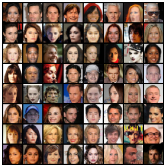
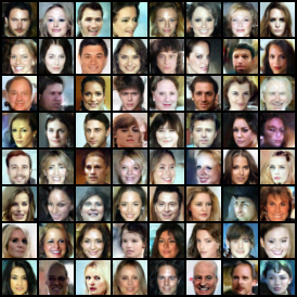
Refer to caption
(a) Ground Truth
Refer to caption
(b) SB-FBSDE Generated Image
Figure 12: Comparison between images generated by ground truth and SB-FBSDE on reduced CelebA. Our SB-FBSDE is trained under the same data pre-processing, network architecture and stepsizes implemented in De Bortoli et al. (2021).
Refer to caption
(a) SGM/50k
Refer to caption
(b) SGM/50k + SB/b/5k
Refer to caption
(c) SGM/50k + SB/f/5k + SB/b/5k
Figure 13: Qualitative results at the different stages of training. (a) Results after 50k training iterations using SGM’s regression loss. (b) Refine the results of Fig. 13a by training the backward policy using (18) with 5k iterations. (c) Refine the results of Fig. 13a with a full SB-FBSDE stage using (18,19).

SGM regression training + SB divergence-based training.

Table 14 reports the FID (using 10k samples, without corrector steps) at different stages of CIFAR10 training. We first train the backward policy with SGM’s regression loss for a sufficient long iterations (50k) until the FID roughly converges. Then, we switch to our alternate training (Alg. 3) using the divergence-based objectives. Crucially, with only 5k iterations of our divergence-based training, we drop the FID dramatically down to 13.35 from 33.68. With a full stage of training (last column), the FID decreases even lower to 11.85. The qualitative results are provided in Fig. 13. Comparing Fig. 13a (corresponds to “SGM/50k” in Table 14) and Fig. 13b (corresponds to “SGM/50k + SB/b/5k” in Table 14), it can be seen that the visible flaw and noise have been substantially improved.

Additional Figures

Figure 14: SGM regression training + SB divergence-based training. We denote “SGM/50k” as “training 50k steps using SGM loss”, and “SB/{f,b}/5k” as “training forward/backward policy with 5k steps using our divergence loss”, and etc.
initialization SGM/10k SGM/20k SGM/50k
SGM/50k
+ SB/b/5k
SGM/50k
+ SB/f/5k + SB/b/5k
FID 448 41.37 35.47 33.68 13.35 11.85
Refer to caption
Figure 15: Uncurated samples generated by our SB-FBSDE on MNIST.
Refer to caption
Figure 16: Uncurated samples generated by our SB-FBSDE on resized CelebA.
Refer to caption
Figure 17: Uncurated samples generated by our SB-FBSDE on CIFAR10.